Embed Size (px)
Citation preview

Performance Tuning and Sizing
Guidelines for Informatica Big Data
Management® 10.2
© Copyright Informatica LLC 2017, 2018. Informatica, the Informatica logo, Big Data Management, Intelligent Data Lake, and Live Data Map are trademarks or registered trademarks of Informatica LLC in the United States and many jurisdictions throughout the world. A current list of Informatica trademarks is available on the web at https://www.informatica.com/trademarks.html.

AbstractYou can tune Big Data Management® for better performance. This article provides sizing recommendations for the Hadoop cluster and the Informatica domain, tuning recommendations for various Big Data Management components, best practices to design efficient mappings, and troubleshooting tips. This article is intended for Big Data Management users, such as Hadoop administrators, Informatica administrators, and Informatica developers.
Supported Versions• Big Data Management 10.2
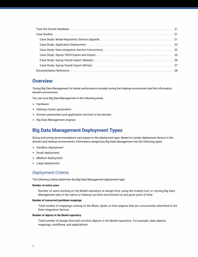
Table of ContentsOverview. . . . . . . . . . . . . . . . . . . . . . . . . . . . . . . . . . . . . . . . . . . . . . . . . . . . . . . . . . . . . . . . . . 3
Big Data Management Deployment Types. . . . . . . . . . . . . . . . . . . . . . . . . . . . . . . . . . . . . . . . . . . . . 3
Deployment Criteria. . . . . . . . . . . . . . . . . . . . . . . . . . . . . . . . . . . . . . . . . . . . . . . . . . . . . . . . . 3
Deployment Type Comparison. . . . . . . . . . . . . . . . . . . . . . . . . . . . . . . . . . . . . . . . . . . . . . . . . . 4
Sizing Recommendations. . . . . . . . . . . . . . . . . . . . . . . . . . . . . . . . . . . . . . . . . . . . . . . . . . . . . . . 5
Hadoop Cluster Hardware Recommendations. . . . . . . . . . . . . . . . . . . . . . . . . . . . . . . . . . . . . . . . 5
Informatica Domain Sizing Recommendations. . . . . . . . . . . . . . . . . . . . . . . . . . . . . . . . . . . . . . . . 6
Intelligent Streaming Sizing and Tuning Recommendations. . . . . . . . . . . . . . . . . . . . . . . . . . . . . . . . . 6
Tune the Hardware and the Hadoop Cluster. . . . . . . . . . . . . . . . . . . . . . . . . . . . . . . . . . . . . . . . . . . 6
Tune the Informatica Domain and Application Services. . . . . . . . . . . . . . . . . . . . . . . . . . . . . . . . . . . . 7
Model Repository Service. . . . . . . . . . . . . . . . . . . . . . . . . . . . . . . . . . . . . . . . . . . . . . . . . . . . . 8
Data Integration Service. . . . . . . . . . . . . . . . . . . . . . . . . . . . . . . . . . . . . . . . . . . . . . . . . . . . . . 8
Analyst Service. . . . . . . . . . . . . . . . . . . . . . . . . . . . . . . . . . . . . . . . . . . . . . . . . . . . . . . . . . . . 9
Search Service. . . . . . . . . . . . . . . . . . . . . . . . . . . . . . . . . . . . . . . . . . . . . . . . . . . . . . . . . . . . 9
Content Management Service. . . . . . . . . . . . . . . . . . . . . . . . . . . . . . . . . . . . . . . . . . . . . . . . . . 10
Tune the Blaze Engine. . . . . . . . . . . . . . . . . . . . . . . . . . . . . . . . . . . . . . . . . . . . . . . . . . . . . . . . 10
Mapping Optimization. . . . . . . . . . . . . . . . . . . . . . . . . . . . . . . . . . . . . . . . . . . . . . . . . . . . . . . 10
Transformation Optimization. . . . . . . . . . . . . . . . . . . . . . . . . . . . . . . . . . . . . . . . . . . . . . . . . . 11
Filter Optimization for Hive Sources. . . . . . . . . . . . . . . . . . . . . . . . . . . . . . . . . . . . . . . . . . . . . . 14
Tune the Spark Engine. . . . . . . . . . . . . . . . . . . . . . . . . . . . . . . . . . . . . . . . . . . . . . . . . . . . . . . . 15
Spark Configuration. . . . . . . . . . . . . . . . . . . . . . . . . . . . . . . . . . . . . . . . . . . . . . . . . . . . . . . . 15
Joiner Transformation Optimization. . . . . . . . . . . . . . . . . . . . . . . . . . . . . . . . . . . . . . . . . . . . . . 16
Troubleshooting Spark Job Failures. . . . . . . . . . . . . . . . . . . . . . . . . . . . . . . . . . . . . . . . . . . . . . 16
Tune the Sqoop Parameters. . . . . . . . . . . . . . . . . . . . . . . . . . . . . . . . . . . . . . . . . . . . . . . . . . . . . 18
Sqoop Command Line Arguments. . . . . . . . . . . . . . . . . . . . . . . . . . . . . . . . . . . . . . . . . . . . . . . 18
Sqoop Tuning Guidelines. . . . . . . . . . . . . . . . . . . . . . . . . . . . . . . . . . . . . . . . . . . . . . . . . . . . . 19
Tune the TDCH for Sqoop Parameters. . . . . . . . . . . . . . . . . . . . . . . . . . . . . . . . . . . . . . . . . . . . . . 19
TDCH for Sqoop Tuning Tips. . . . . . . . . . . . . . . . . . . . . . . . . . . . . . . . . . . . . . . . . . . . . . . . . . 20
TDCH for Sqoop Import and Export Guidelines. . . . . . . . . . . . . . . . . . . . . . . . . . . . . . . . . . . . . . . 21
2
Tune the Oracle Database. . . . . . . . . . . . . . . . . . . . . . . . . . . . . . . . . . . . . . . . . . . . . . . . . . . . . . 21
Case Studies. . . . . . . . . . . . . . . . . . . . . . . . . . . . . . . . . . . . . . . . . . . . . . . . . . . . . . . . . . . . . . 21
Case Study: Model Repository Service Upgrade. . . . . . . . . . . . . . . . . . . . . . . . . . . . . . . . . . . . . . 21
Case Study: Application Deployment. . . . . . . . . . . . . . . . . . . . . . . . . . . . . . . . . . . . . . . . . . . . . 22
Case Study: Data Integration Service Concurrency. . . . . . . . . . . . . . . . . . . . . . . . . . . . . . . . . . . . . 23
Case Study: Sqoop TDCH Export and Import. . . . . . . . . . . . . . . . . . . . . . . . . . . . . . . . . . . . . . . . 25
Case Study: Sqoop Oracle Import (Reader). . . . . . . . . . . . . . . . . . . . . . . . . . . . . . . . . . . . . . . . . 26
Case Study: Sqoop Oracle Export (Writer). . . . . . . . . . . . . . . . . . . . . . . . . . . . . . . . . . . . . . . . . . 27
Documentation Reference. . . . . . . . . . . . . . . . . . . . . . . . . . . . . . . . . . . . . . . . . . . . . . . . . . . . . . 28
OverviewTuning Big Data Management for better performance includes tuning the Hadoop environment and the Informatica domain environment.
You can tune Big Data Management in the following areas:
• Hardware
• Hadoop cluster parameters
• Domain parameters and application services in the domain
• Big Data Management engines
Big Data Management Deployment TypesSizing and tuning recommendations vary based on the deployment type. Based on certain deployment factors in the domain and Hadoop environments, Informatica categorizes Big Data Management into the following types:
• Sandbox deployment
• Small deployment
• Medium deployment
• Large deployment
Deployment CriteriaThe following criteria determine the Big Data Management deployment type:
Number of active users
Number of users working on the Model repository at design time, using the Analyst tool, or running Big Data Management jobs in the native or Hadoop run-time environment at any given point of time.
Number of concurrent pushdown mappings
Total number of mappings running on the Blaze, Spark, or Hive engines that are concurrently submitted to the Data Integration Service.
Number of objects in the Model repository
Total number of design-time and run-time objects in the Model repository. For example, data objects, mappings, workflows, and applications.
3

Number of deployed applications
Total number of applications deployed across all the Data Integration Services in the Informatica domain.
Number of objects per application
Total number of objects of all types that are deployed as part of a single application.
Total operational data volume
Total volume of data being processed in the Hadoop environment at any given point of time.
Total number of data nodes
Total number of data nodes in the Hadoop cluster.
yarn.nodemanager.resource.cpu-vcores
A property in the yarn-site.xml on the Hadoop cluster that specifies the number of virtual cores for containers.
yarn.nodemanager.resource.memory-mb
A property in the yarn-site.xml on the Hadoop cluster that specifies the maximum physical memory available for containers.
Deployment Type ComparisonThe following table compares Big Data Management deployment types based on the standard values for each deployment factor:
Deployment Factor Sandbox Deployment
Small Deployment
Medium Deployment
Large Deployment
Domain environment
Number of active users 1 5 10 50
Number of concurrent pushdown mappings < 10 20 -500 500 - 1000 > 1000
Number of objects in the Model repository < 1000 < 5000 < 20,000 20,000 +
Number of deployed applications < 10 < 25 < 100 < 500
Number of objects per application < 10 10 - 50 50 -100 50 -100
Total operational data volume(for batch processing use cases)
10 GB 100 GB 500 GB 1 TB +
Messages processed per second(for streaming use cases with Informatica Intelligent Streaming)
100,000 500,000 1 Million 10 Million
Hadoop environment
Total number of data nodes 3 5 8 - 12 12 +
yarn.nodemanager.resource.cpu-vcores 12 24 24 36
yarn.nodemanager.resource.memory-mb 12288 MB 24576 MB 49152 MB 98304 MB
4

Sizing RecommendationsBased on your Big Data Management deployment type, use the sizing guidelines for the Hadoop and domain environments.
Hadoop Cluster Hardware RecommendationsThe following table lists the minimum and optimal hardware requirements for the Hadoop cluster:
Hardware Sandbox Deployment
Small or Medium Deployment
Large Deployment
CPU speed 2 - 2.5 GHz 2 - 2.5 GHz 2.5 - 3.5 GHz
Logical or virtual CPU cores 16 24 - 32 48
Total system memory 16 GB 64 GB 128 GB
Local disk space for yarn.nodemanager.local-dirs1
256 GB 500 GB 2.4 TB
DFS block size 128 MB 256 MB 256 MB
HDFS replication factor 3 3 3
Disk capacity 32 GB 256 GB - 1 TB 1.2 TB
Total number of disks for HDFS 2 8 12
Total HDFS capacity per node 64 GB 2 - 8 TB At least 14.4 TB
Number of nodes 2 + 4 - 10+ 12 +
Total HDFS capacity on the cluster 128 GB 8 - 80 TB 144 TB
Actual HDFS capacity (with replication) 43 GB 2.66 TB 57.6 TB
/tmp mount point 20 GB 20 GB 30 GB
Installation disk space requirement 12 GB 12 GB 12 GB
Network bandwidth (Ethernet card) 1 Gbps 2 Gbps (bonded channel) 10 Gbps (Ethernet card)
1 A property in the yarn-site.xml that contains a list of directories to store localized files. You can find the localized file directory in: ${yarn.nodemanager.local-dirs}/usercache/${user}/appcache/application_${appid}. You can find the work directories of individual containers, container_${contid}, as the subdirectories of the localized file directory.
MapR Cluster Recommendation
When you run mappings on the Blaze, Spark, or Hive engine, local cache files are generated under the directory specified in the yarn.nodemanager.local-dirs property in the yarn-site.xml. However, the directory might not contain sufficient disk capacity on a MapR cluster.
To make sure that the directory has sufficient disk capacity, perform the following steps:
1. Create a volume on HDFS.
5

2. Mount the volume through NFS.
3. Configure the NFS mount location in yarn.nodemanager.local-dirs.
For more information, refer to the MapR documentation.
Informatica Domain Sizing RecommendationsThe following table lists the minimum hardware requirements for the server on which the Informatica domain runs:
Hardware Sandbox Deployment Small Deployment Medium Deployment Large Deployment
Total CPU cores1 16 24 36 96
Total system memory 32 GB 32 GB 64 GB 128 GB
Disk space per node2 50 GB 100 GB + 100 GB + 100 GB +
1 CPU cores are physical cores.
2 Disk space requirement is for Informatica services. Additional disk capacity is required to process data in the native run-time environment.
Intelligent Streaming Sizing and Tuning RecommendationsUse Informatica Intelligent Streaming mappings to collect streaming data, build the business logic for the data, and push the logic to a Spark engine for processing. The Spark engine uses Spark Streaming to process data. Streaming mapping includes streaming sources such as Kafka or JMS. The Spark engine reads the data, divides the data into micro batches, and publishes it.
Streaming mappings run continuously. When you create and run a streaming mapping, a Spark application is created on the Hadoop cluster which runs forever unless killed or cancelled through the Data Integration Service. Because a batch is triggered for every micro batch interval that is configured for the mapping, consider the following recommendations:
• The processing time for each batch must remain the same over the entire duration.
• The batch processing time of every batch must be less than batch interval.
For more sizing and tuning recommendations, refer to the following Informatica How-To Library article:
Sizing Guidelines and Performance Tuning for Intelligent Streaming
Tune the Hardware and the Hadoop ClusterTune the following hardware parameters for better performance:
• CPU frequency
• NIC card ring buffer size
Tune the following Hadoop cluster parameters for better performance:
• Hard disk
• Transparent huge page
• HDFS block size
• HDFS access timeout
6
• YARN settings for parallel jobs
For more information, refer to the following Informatica How-to Library article:
Tuning the Hardware and Hadoop Clusters for Informatica Big Data Products
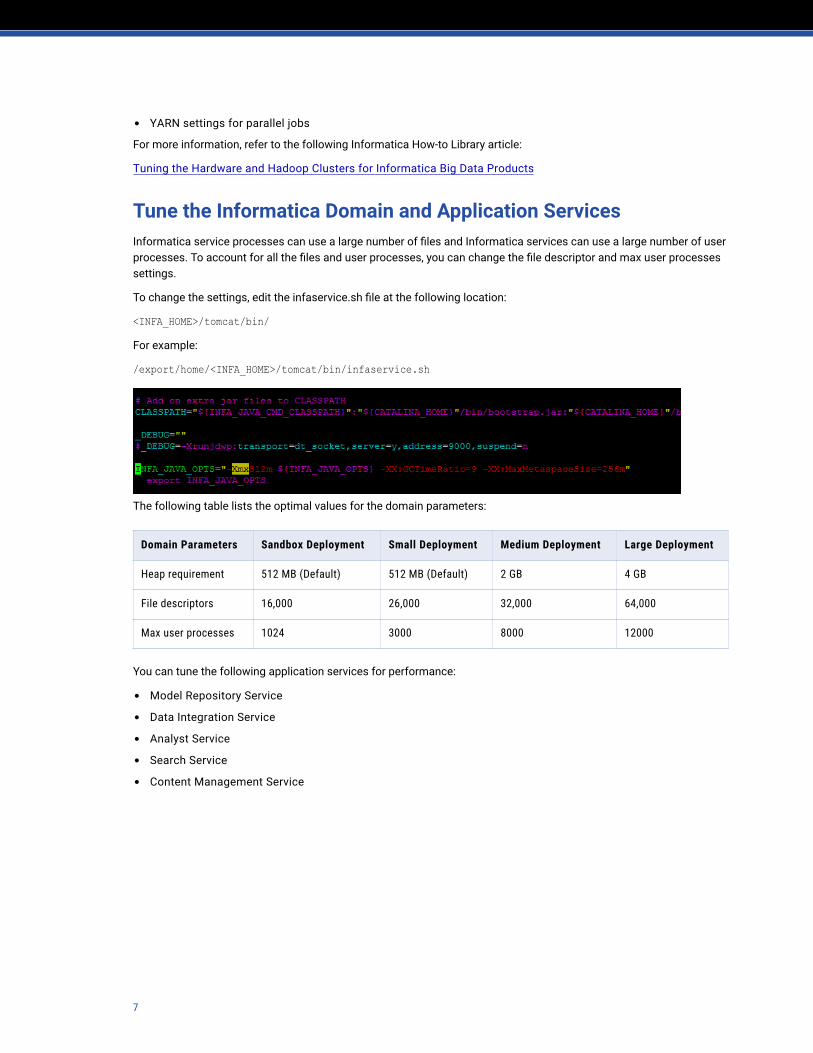
Tune the Informatica Domain and Application ServicesInformatica service processes can use a large number of files and Informatica services can use a large number of user processes. To account for all the files and user processes, you can change the file descriptor and max user processes settings.
To change the settings, edit the infaservice.sh file at the following location:
<INFA_HOME>/tomcat/bin/
For example:
/export/home/<INFA_HOME>/tomcat/bin/infaservice.sh
The following table lists the optimal values for the domain parameters:
Domain Parameters Sandbox Deployment Small Deployment Medium Deployment Large Deployment
Heap requirement 512 MB (Default) 512 MB (Default) 2 GB 4 GB
File descriptors 16,000 26,000 32,000 64,000
Max user processes 1024 3000 8000 12000
You can tune the following application services for performance:
• Model Repository Service
• Data Integration Service
• Analyst Service
• Search Service
• Content Management Service
7

Model Repository ServiceYou can tune the maximum heap size for the Model Repository Service and the heap size required to store the monitoring configuration in the Model repository.
The following table lists the guidelines to tune the heap sizes:
Parameter Sandbox Deployment Small Deployment Medium Deployment Large Deployment
Max heap size 1 GB 1 GB 2 GB 4 GB
Max heap size for monitoring
1 GB 1 GB 2 GB 4 GB
Note: The heap size requirements on the Model Repository Service is primarily driven by the number of simultaneous save, fetch, and delete operations and the number of concurrent mapping executions. The Model Repository Service actions, such as application deploy, redeploy, import, and export, also affect the heap size memory requirements and the efficiency of design-time operations.
Additional Guidelines
Informatica recommends the following additional guidelines for the Model Repository Service:
• Create a separate Model Repository Service for monitoring statistics.
• Schedule a periodic purge of monitoring statistics and retain only the required statistics.
• When you upgrade the Model Repository Service, it requires a minimum of 4 GB heap memory.
Data Integration ServiceYou can configure the maximum heap size and the batch execution pool sizes for the Hadoop and native environments.
The following table lists the recommended values for the Data Integration Service parameters:
Parameter Sandbox Deployment
Small Deployment
Medium Deployment
Large Deployment
Max heap size 640 MB 2 GB 2 - 4 GB 4 - 6 GB
Execution pool size for the Hadoop environment
10 500 1000 2000+
Execution pool size for the native environment
10 10 15 30
Note: The number of concurrent pushdown jobs submitted to the Data Integration Service determine the heap size and the execution pool size.
Additional Guidelines
Informatica recommends the following additional guidelines for the Data Integration Service:
• Application deployment requires communication between the Data Integration Service and the associated Model Repository Service. To fetch objects and to write to the database schema of the Model Repository Service, tune the database cursors as follows:
Number of database cursors >= Number of objects in the application
8

• To run jobs in the native environment and to preview data, the Data Integration Service requires at least one physical core for each job execution.
• If the Data Integration Service is enabled to use multiple partitions for native jobs, the Data Integration Service node resource requirements increase based on the parallelism. If the number of jobs in the native environment are typically high, you must allocate additional resources for other jobs.
Profiling Parameters
Informatica recommends that you perform profiling using the Blaze engine for performance considerations. Tuning profiling performance involves configuring the data integration service parameters, the profile database warehouse properties, and the advanced profiling properties.
For more information, see the "Tuning for Profiling Performance," "Tuning Profile Warehouse," and "Profile Warehouse Guidelines for Column Profiling" sections in the Tuning Live Data Map Performance How-to Library article located at:
https://kb.informatica.com/h2l/HowTo%20Library/1/Live%20Data%20Map%20Performance%20Tuning%20Guide=1=PDF%20(H2L)=en.pdf
Analyst ServiceYou can tune the maximum heap size for the Analyst Service.
The following table lists the guidelines to tune the heap sizes:
Parameter Sandbox Deployment Small Deployment Medium Deployment Large Deployment
Max heap size 768 MB 1 GB 2 GB 4 GB
Note: The number of active concurrent users working on the Analyst tool and the number of objects processed per user determine the heap size.
Search ServiceYou can tune the maximum heap size for the Search Service.
The following table lists the guidelines to tune the heap sizes:
Parameter Sandbox Deployment Small Deployment Medium Deployment Large Deployment
Max heap size 768 MB 1 GB 2 GB 4 GB
Note: The size of the Model Repository Service and the profiling warehouse and the volume of business glossary data being processed determine the heap size.
9

The following table lists additional Search Service properties that you can tune:
Parameter Description and Recommendation
Index Location Directory that contains the search index files.To save index files, you allocate disk space on one of the nodes in the domain. Make sure that the disk location has enough space to write index files.Recommendation: Disk space must be approximately twice the size of the schema.
Extraction Interval
Interval in seconds at which the Search Service updates the search index. The Search Service checks for changes in the metadata before reindexing. Default extraction interval is 60 seconds.Recommendation: The extraction interval must be greater than or equal to the time taken to complete indexing the first time.
Content Management ServiceYou can tune the maximum heap size for the Content Management Service.
The following table lists the guidelines to tune the heap sizes:
Parameter Sandbox Deployment Small Deployment Medium Deployment Large Deployment
Max heap size 1 GB 2 GB 4 GB 4 GB
Note: The number and size of the reference tables determine the heap size.
Tune the Blaze EngineWhen you develop mappings in the Developer tool to run on the Blaze engine, consider the following tuning recommendations and performance best practices.
Mapping OptimizationConsider the following best practices when you develop mappings to run on the Blaze engine:
Tune port precision values.
If the precision value in a string port is unnecessarily large, more buffer memory is allocated instead of what is actually required. Larger cache in the disk results in high I/O overhead and causes severe performance degradation. Larger cache also causes data to spill to the disks which might result in eventual failures due to inadequate disk space.
Performance best practice: Use string port with large precision values only when required.
Avoid unnecessary data type conversions.
Mismatched port data types and mismatched port precisions increase the computational overhead. Ensure that the port precisions and data types are consistent across sources, transformations, and targets within a mapping.
10
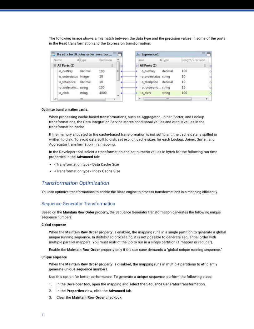
The following image shows a mismatch between the data type and the precision values in some of the ports in the Read transformation and the Expression transformation:
Optimize transformation cache.
When processing cache-based transformations, such as Aggregator, Joiner, Sorter, and Lookup transformations, the Data Integration Service stores conditional values and output values in the transformation cache.
If the memory allocated to the cache-based transformation is not sufficient, the cache data is spilled or written to disk. To avoid data spill to disk, set explicit cache sizes for each Lookup, Joiner, Sorter, and Aggregator transformation in a mapping.
In the Developer tool, select a transformation and set numeric values in bytes for the following run-time properties in the Advanced tab:
• <Transformation type> Data Cache Size
• <Transformation type> Index Cache Size
Transformation OptimizationYou can optimize transformations to enable the Blaze engine to process transformations in a mapping efficiently.
Sequence Generator Transformation
Based on the Maintain Row Order property, the Sequence Generator transformation generates the following unique sequence numbers:
Global sequence
When the Maintain Row Order property is enabled, the mapping runs in a single partition to generate a global unique running sequence. In distributed processing, it is not possible to generate sequential order with multiple parallel mappers. You must restrict the job to run in a single partition (1 mapper or reducer).
Enable the Maintain Row Order property only if the use case demands a "global unique running sequence."
Unique sequence
When the Maintain Row Order property is disabled, the mapping runs in multiple partitions to efficiently generate unique sequence numbers.
Use this option for better performance. To generate a unique sequence, perform the following steps:
1. In the Developer tool, open the mapping and select the Sequence Generator transformation.
2. In the Properties view, click the Advanced tab.
3. Clear the Maintain Row Order checkbox.
11

The following image shows the Advanced tab of a Sequence Generator transformation:
Data Processor Transformation
Consider the following best practices for mappings that contain a Data Processor transformation:
• For mappings that run on the Blaze engine, it is required to enable partitioning for Data Processor transformations. To enable partitioning, perform the following steps:
1. In the Developer tool, open the mapping and select the Data Processor transformation.
2. In the Properties view, click the Advanced tab.
3. Select Enable partitioning for Data Processor transformations.The following image shows the Advanced tab of a Data Processor transformation:
• When a mapping with a Data Processor transformation meets all of the following conditions, the Blaze engine processes the entire mapping in a single tasklet:
- The mapping source file is of a non-splittable input format.
- The transformation contains multiple output groups.
12

The Data Processor transformation might output a higher data volume than the source. For such scenarios, configure the Blaze engine to first stage the data generated by the transformation at each output group.
The following image shows a mapping with a Data Processor transformation with multiple output groups:
To stage data at every output group, set the following mapping run-time property in the Developer tool:
Parameter Value
Blaze.StageOutputGroupDataForInstances The name of the Data Processor transformation instance.
When the Blaze engine is configured to first stage the data, it performs the following tasks:
- Re-partitions the data.
- Processes the staged data.
- Creates the correct number of tasklets based on the staged data volume.
Aggregator Transformation
Disable map-side aggregation if a unique key is used as the group by key in an Aggregator transformation.
In the Blaze engine, map-side aggregation is analogous to the aggregation done in the map phase in a MapReduce job that runs on the Hive engine. Source data is aggregated based on the group-by port set in an Aggregator transformation. The aggregated data then moves to the data shuffle stage for the second level of aggregation.
If you specify a unique key as the group by port, disable the map-side aggregation in a mapping that runs on the Blaze engine.
13

In the Developer tool, set the following run-time property in the Run-time tab to disable map-side aggregation for the mapping:
Parameter Value
GridExecutor.EnableMapSideAgg False
Filter Optimization for Hive SourcesTo optimize mappings that read from a partitioned Hive source, you typically add filter conditions on a relational data object to remove rows at the source. The filter limits the data that flows through the mapping pipeline which gives a performance benefit. However, when the Blaze engine reads from a Hive source with a filter condition, the engine interprets the filters as SQL overrides, translates into multiple grid tasks, and adds a performance overhead.
The Blaze engine translates the filters into the following grid tasks:
• A grid task to create a HiveServer2 job for the filter override to stage the intermediate data.
• A grid task to operate against the staged data and to apply the downstream mapping logic.
For example, the following image shows the Blaze engine execution plan with two grid tasks for a passthrough mapping with a filter:
To avoid the performance overhead, set the following custom flag as an advanced property of the mapping:
Hive.SourceFilterAsInfaExpression = trueIf multiple mappings require the flag, add the custom flag at the Data Integration Service level.
The following image shows the custom flag that you added as an execution parameter for the mapping:
14

The following image shows the Blaze engine execution plan with a single grid task after you set the custom flag:
Note: Use a valid Informatica expression as a filter condition. The filter condition must not refer to the table name. For example, instead of LineItem.l_tax > $dataasofdate, use l_tax > $dataasofdate.
The following image shows the Query view of the relational data object where you define the filter condition:
Tune the Spark EngineWhen you develop mappings in the Developer tool to run on the Spark engine, consider the following prerequisites, tuning recommendations, and performance best practices.
Meet the following prerequisites:
• On the Hadoop cluster, configure the Spark History Server.
• On the Hadoop cluster, enable the Spark Shuffle Service.
• In the Hadoop connection to run mappings on the Spark engine, set up the Spark History Server, Spark HDFS staging directory, and Spark event log directory.
For more information about configuring Spark History Server and Spark Shuffle Service, refer to the Hadoop distribution documentation.
For more information about configuring the Hadoop connection, refer to the Informatica Big Data Management User Guide.
Spark ConfigurationThe properties for the Spark engine are tuned in the hadoopEnv.properties file.
The hadoopEnv.properties file is located at:
<Informatica installation directory>/services/shared/hadoop/<Hadoop distribution name>/infaConf
15

The values in the file are tuned for large deployment types. The following table lists the tuning recommendations for sandbox, small, and medium deployment types:
Property Sandbox and Small Deployments
Medium Deployment Large Deployment (Default)
spark.executor.memory 2 GB 4 GB 6 GB
spark.executor.cores 2 2 2
Infaspark.shuffle.max.partitions1
(8 * per GB data at shuffle)800 4000 8000
spark.driver.memory2 1 GB 2 GB 4 GB + (default)
spark.driver.maxResultSize 1 GB 2 GB 4 GB + (default)
1 Infaspark.shuffle.max.partitions
Sets the number of shuffle partitions to the maximum number of partitions seen across all input sources.
Recommended value: Allocate approximately eight dynamic shuffle partitions for each gigabyte of shuffle data. For example, for 400 GB of shuffle data, set this value to 3200.
2 spark.driver.memory
Sets the driver process memory to a default value of 4 GB. The driver requires more memory based on the number of data sources and data nodes.
Recommended value: Allocate at least 256 MB for every data source participating in map join. For example, if a mapping has eight data sources, set the driver memory to at least 2 GB (8 x 256).
Joiner Transformation OptimizationYou can optimize Joiner transformations to enable the Spark engine to efficiently perform a full outer join.
To increase memory for a full outer join and to determine shuffle partitions, perform the following two-step tuning process:
1. Ensure every executor core has at least 3 GB of memory.For example, set spark.executor.memory=6 GB and spark.executor.cores=2.
2. Set spark.sql.shuffle.partitions = <master splits> + <detailed partitions>.The spark.sql.shuffle.partitions property determines the number of partitions to use when shuffling data for joins or aggregations.
For example, with a DFS block size of 256 MB, 100 GB of master data will have 400 splits and 200 GB of details will have 800 partitions.
Troubleshooting Spark Job FailuresThis section provides information on troubleshooting common error messages and limitations that you might encounter when you enable dynamic resource allocation on the Spark engine. These errors might occur when you process a large volume of data, such as 10 TB or more, or when a job has a large shuffle volume.
Could not find CoarseGrainedScheduler.
When you stop a process, you might lose one or more executors with the following error:
cluster.YarnScheduler: Lost executor 8 on myhost1.com: remote Rpc client disassociated
16

One of the most common reasons for executor failure is insufficient memory. When an executor consumes more memory than the maximum limit, YARN causes the executor to fail. By default, Spark does not set an upper limit for the number of executors if dynamic allocation is enabled. (SPARK-14228)
In the hadoopEnv.properties file, configure the following properties:
Property Description
spark.dynamicAllocation.maxExecutors Set a limit for the number of executors. Determine the value based on available cores and memory per node.
spark.executor.memory Increase the amount of memory per executor process. The default value is 6 GB.
Total size of serialized results is bigger than spark.driver.maxResultSize.
The spark.driver.maxResultSize property determines the limit for total size of serialized results across all partitions for each Spark action, such as the collect action. Spark driver issues a collect() for the whole broadcast data set. The spark default of 1 GB is overridden and increased to 4 GB. This value should suffice most use cases. If the spark driver fails with the following error message, consider increasing this value:
Total size of serialized results is bigger than spark.driver.maxResultSizeIn the hadoopEnv.properties file, configure the following property:
Property Description
spark.driver.maxResultSize Set the result size to a size equal to or greater than the driver memory, or 0 for unlimited.
java.util.concurrent.TimeoutException; Futures timed out after [300 seconds].
The default broadcast timeout limit is set to 300 seconds. Increase the SQL broadcast timeout limit.
In the hadoopEnv.properties file, configure the following property:
Property Description
spark.sql.broadcastTimeout Set the timeout limit to at least 600 seconds.
A job fails due to Spark speculative execution of tasks.
With spark speculation, the Spark engine relaunches one or more tasks that are running slowly in a stage. To successfully run the job, disable spark speculation.
In the hadoopEnv.properties file, configure the following property:
Property Description
spark.speculation Set the value to false.
ShuffleMapStage 12 (rdd at InfaSprk1.scala:48) has failed the maximum allowable number of times: 4.
The Spark shuffle service fails because the garbage collector exceeded the overhead limit. This forces the Node Manager to shut down, which eventually causes the Spark job to fail.
17

To resolve this issue, perform the following steps:
1. Open the YARN node manager.
2. In the NodeManager Java heap size property, increase the maximum heap size in MB.
For further debugging, check the Node Manager logs:
java.lang.OutOfMemoryError : GC overhead limit exceeded 2016-12-0 7 19:38:29,934 FATAL yarn.YarnUncaughtExceptionHandler(YarnUncaughtExceptionHandler.java:uncaughtException 51))- Thread Thread[IPCServer handler 0on 8040,5,main] threwan error. Shutting down now...
Tune the Sqoop ParametersUse Sqoop to process data between relational databases and HDFS through MapReduce programs. You can use Sqoop to import and export data. When you use Sqoop, you do not need to install the relational database client and software on any node in the Hadoop cluster.
Sqoop Command Line ArgumentsYou can tune certain parameters to optimize performance of Sqoop readers and writers. Add the parameters in the JDBC connection or to Sqoop mappings.
The following table lists the parameters that you can tune:
Parameter Applies To Description
batch Writer Specifies that you can group the related SQL statements into a batch when you export data.
direct Reader and writer
Specifies the direct import fast path when you import data from a relational source.Note: Applies to Oracle and TDCH connectors.
Dsqoop.export.records.per.statement Writer Specifies to insert multiple rows with a single statement.
Enable primary key Reader Enables the primary key constraint on the source table to optimize performance when reading data from a source.
fetch-size Reader Specifies the number of entries that Sqoop can import at a time.
num-mapper Reader and writer
Specifies the number of map tasks that can run in parallel.
compress or z Reader Enables compression.
Dmapreduce.map.java.opts Reader Specifies the Java options per statement if Java runs out of memory.
Dmapred.child.java.opts Reader Specifies the Java options per mapper if Java runs out of memory.
18
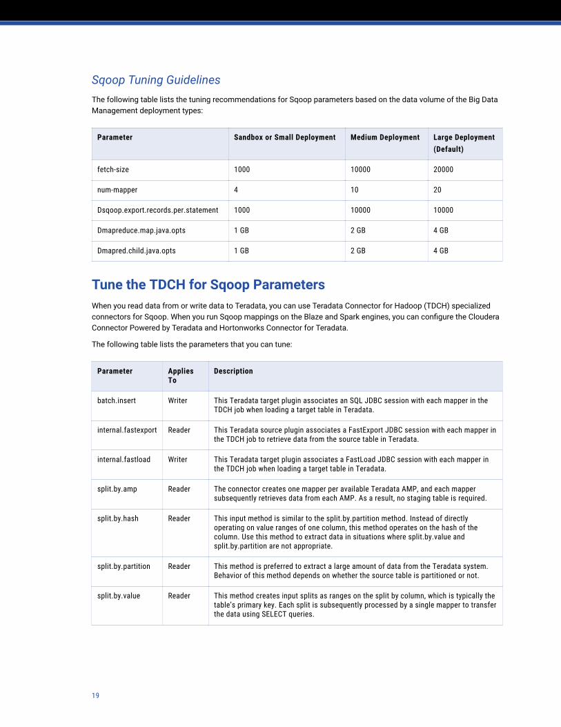
Sqoop Tuning GuidelinesThe following table lists the tuning recommendations for Sqoop parameters based on the data volume of the Big Data Management deployment types:
Parameter Sandbox or Small Deployment Medium Deployment Large Deployment(Default)
fetch-size 1000 10000 20000
num-mapper 4 10 20
Dsqoop.export.records.per.statement 1000 10000 10000
Dmapreduce.map.java.opts 1 GB 2 GB 4 GB
Dmapred.child.java.opts 1 GB 2 GB 4 GB
Tune the TDCH for Sqoop ParametersWhen you read data from or write data to Teradata, you can use Teradata Connector for Hadoop (TDCH) specialized connectors for Sqoop. When you run Sqoop mappings on the Blaze and Spark engines, you can configure the Cloudera Connector Powered by Teradata and Hortonworks Connector for Teradata.
The following table lists the parameters that you can tune:
Parameter Applies To
Description
batch.insert Writer This Teradata target plugin associates an SQL JDBC session with each mapper in the TDCH job when loading a target table in Teradata.
internal.fastexport Reader This Teradata source plugin associates a FastExport JDBC session with each mapper in the TDCH job to retrieve data from the source table in Teradata.
internal.fastload Writer This Teradata target plugin associates a FastLoad JDBC session with each mapper in the TDCH job when loading a target table in Teradata.
split.by.amp Reader The connector creates one mapper per available Teradata AMP, and each mapper subsequently retrieves data from each AMP. As a result, no staging table is required.
split.by.hash Reader This input method is similar to the split.by.partition method. Instead of directly operating on value ranges of one column, this method operates on the hash of the column. Use this method to extract data in situations where split.by.value and split.by.partition are not appropriate.
split.by.partition Reader This method is preferred to extract a large amount of data from the Teradata system. Behavior of this method depends on whether the source table is partitioned or not.
split.by.value Reader This method creates input splits as ranges on the split by column, which is typically the table’s primary key. Each split is subsequently processed by a single mapper to transfer the data using SELECT queries.
19
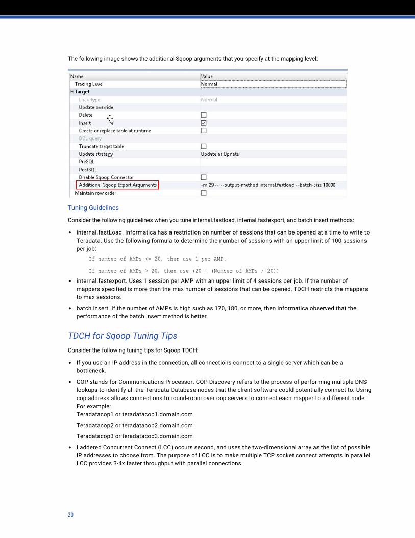
The following image shows the additional Sqoop arguments that you specify at the mapping level:
Tuning Guidelines
Consider the following guidelines when you tune internal.fastload, internal.fastexport, and batch.insert methods:
• internal.fastLoad. Informatica has a restriction on number of sessions that can be opened at a time to write to Teradata. Use the following formula to determine the number of sessions with an upper limit of 100 sessions per job:
If number of AMPs <= 20, then use 1 per AMP.
If number of AMPs > 20, then use (20 + (Number of AMPs / 20))• internal.fastexport. Uses 1 session per AMP with an upper limit of 4 sessions per job. If the number of
mappers specified is more than the max number of sessions that can be opened, TDCH restricts the mappers to max sessions.
• batch.insert. If the number of AMPs is high such as 170, 180, or more, then Informatica observed that the performance of the batch.insert method is better.
TDCH for Sqoop Tuning TipsConsider the following tuning tips for Sqoop TDCH:
• If you use an IP address in the connection, all connections connect to a single server which can be a bottleneck.
• COP stands for Communications Processor. COP Discovery refers to the process of performing multiple DNS lookups to identify all the Teradata Database nodes that the client software could potentially connect to. Using cop address allows connections to round-robin over cop servers to connect each mapper to a different node. For example:Teradatacop1 or teradatacop1.domain.com
Teradatacop2 or teradatacop2.domain.com
Teradatacop3 or teradatacop3.domain.com
• Laddered Concurrent Connect (LCC) occurs second, and uses the two-dimensional array as the list of possible IP addresses to choose from. The purpose of LCC is to make multiple TCP socket connect attempts in parallel. LCC provides 3-4x faster throughput with parallel connections.
20

TDCH for Sqoop Import and Export GuidelinesSpark job scales linearly during Sqoop import and export. You can tune Spark jobs based on cluster resources. In the hadoopEnv.properties file, add the following property:
spark.executor.instances=<number of executor instances>
The following formula determines the total running containers:
Total running containers = (Number of cores) x (Number of executor instances)
The Spark engine uses 2 executor instances by default. So, only 4 containers run in parallel. For better performance, fine tune the spark.executor.instances property.
Tune the Oracle DatabaseTo optimize the performance of Oracle databases, perform the following tasks:
• Analyze database statistics to fine tune queries.
• Maintain different physical disks for different tablespaces.
• Determine the expected database growth.
• Use the EXPLAIN PLAN statement to fine tune queries.
• Avoid foreign key constraints.
• Drop indexes before loading data.
• Set open cursors and sessions optimally for mappers to process queries in parallel.
Case StudiesRefer to the following case studies for a general idea on the performance numbers.
Case Study: Model Repository Service UpgradeModel Repository Service upgrade time depends on the number of objects in the repository. Larger backup file size means more time to upgrade. A minimum of 4GB heap memory is required for Model Repository Service during the upgrade process.
Test Setup
Chipset Intel® Xeon® CPU E5-4650 0 @ 2.70GHz
Cores 32 cores
Memory 128 GB
Operating system RedHat Enterprise Linux 6.5
21

Performance Chart
The following chart shows the time taken to upgrade Model Repository Services from Big Data Management 9.6.1 to 10.2:
Case Study: Application DeploymentApplication deployment requires communication between the Data Integration Service and the associated Model Repository Service. The Data Integration Service fetches the object and writes to the database schema of the Model Repository Service.
Test Setup
Chipset Intel® Xeon® CPU E5-4650 0 @ 2.70GHz
Cores 32 cores
Memory 128 GB
Operating system RedHat Enterprise Linux 6.5
22

Performance Chart
The following chart shows the time taken to deploy applications with a different number of objects:
Conclusions
Based on the case study, Informatica recommends the following best practices for application deployment when you have a similar configuration:
Number of objects in applications
Having a large number of objects in the same application is not desirable. It increases the deployment time. It also increases the resource usage of the Data Integration Service and the Model Repository Service. Distributing objects in an optimal manner between various applications is key to achieve better performance.
Recommendation: ~ 50 objects per application.
Workaround for incremental application deployment
To deploy the changes made to the application, you stop the application and redeploy it. This process causes downtime. Applications must be designed to minimize the effects on this downtime. If the number of objects in the application are less, the effect of the downtime will be less severe. Thus, an application must not be designed with too many objects within.
Recommendation: ~ 50 objects per application.
Cursor requirements on the database
The process of application deployment needs to use cursors at the database layer (the schema associated with the Model Repository service). If applications are designed to be too large (1000+ of objects within) or with deep hierarchy of objects, the cursor usage will be greater at the database level.
Recommendation: Required number of cursors >= Number of objects in application.
Case Study: Data Integration Service ConcurrencyA single Data Integration Service in Informatica Big Data management can handle hundreds and thousands of concurrent pushdown mappings. The following case study shows that the Data Integration Service with 4 GB heap memory can dispatch up to 500 concurrent mappings of TPC-DS benchmark queries of medium complexity in ~15 minutes.
23

Test Setup
Chipset Intel® Xeon® Processor X5675 @ 3.06 GHz
Cores 2 x 6 cores
Memory 32 GB
Operating system RedHat Enterprise Linux 6.7
Hadoop distribution Hortonworks HDP 2.6
Hadoop cluster 25 nodes
Performance Chart
The Data Integration Service uses Concurrent Mark Sweep Garbage Collection by default. This Garbage Collection is not efficient to handle very large concurrent workloads. The following chart shows the benefits of using G1GC Garbage Collection to process more than 200 concurrent Big Data Management pushdown mappings:
Conclusions
• When you submit concurrent mapping requests, use the infacmd gateway service to optimize performance.For more details, refer to the following Informatica Knowledge Base article:
Gateway Service to Submit Mappings and Workflows to the Data Integration Service
• Set the JVM Command Line Options (on the Processes tab on the Data Integration Service process) as follows:
-Dfile.encoding=UTF-8 -server -Xms256M-XX:+HeapDumpOnOutOfMemoryError -XX:MaxMetaspaceSize=384m-XX:+UseG1GC -XX:MaxGCPauseMillis=500
• For workloads with more than 250 concurrent mappings, Informatica recommends using the Data Integration Service on grid. This configuration reduces dispatch latency when the Data Integration Service processes concurrent mapping requests.
24
• To execute concurrent mappings, set the following custom property for the Data Integration Service in the Administrator tool:
MappingServiceOptions.LdtmCompileMaxConcurrency=Number of virtual cores on the Data Integration Service node
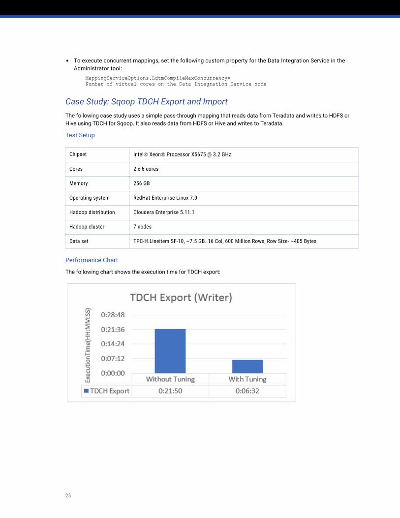
Case Study: Sqoop TDCH Export and ImportThe following case study uses a simple pass-through mapping that reads data from Teradata and writes to HDFS or Hive using TDCH for Sqoop. It also reads data from HDFS or Hive and writes to Teradata.
Test Setup
Chipset Intel® Xeon® Processor X5675 @ 3.2 GHz
Cores 2 x 6 cores
Memory 256 GB
Operating system RedHat Enterprise Linux 7.0
Hadoop distribution Cloudera Enterprise 5.11.1
Hadoop cluster 7 nodes
Data set TPC-H.Lineitem SF-10, ~7.5 GB. 16 Col, 600 Million Rows, Row Size- ~405 Bytes
Performance Chart
The following chart shows the execution time for TDCH export:
25

The following chart shows the execution time for TDCH import:
Conclusions
• For the Sqoop writer, the number of mappers increased from the default 4 to 144. With the maximum session restriction for the internal.fastLoad method, the actual sessions created were 25.
• For the Sqoop reader, the number of mappers increased from the default 1 to 144. Default value is 1 because the table has a primary key defined. When the number of mappers increase, Informatica recommends to set the value of the spark.executor.instances property equal to the number of mappers for optimal performance.
Case Study: Sqoop Oracle Import (Reader)The following case study uses a simple pass-through mapping that reads data from Oracle source and writes to HDFS using Sqoop.
Test Setup
Chipset Intel® Xeon® Processor X5675 @ 3.2 GHz
Cores 2 x 6 cores
Memory 256 GB
Operating system RedHat Enterprise Linux 7.0
Hadoop distribution Cloudera Enterprise 5.11.1
Hadoop cluster 7 nodes
Data set TPC-H.Lineitem SF-100, ~75 GB. 16 Col, 6 Billion Rows, Row Size- ~405 Bytes
26

Performance Chart
The following chart shows the execution time for Oracle import:
Case Study: Sqoop Oracle Export (Writer)The following case study uses a simple pass-through mapping that reads data from HDFS and writes to Oracle using Sqoop.
Test Setup
Chipset Intel® Xeon® Processor X5675 @ 3.2 GHz
Cores 2 x 6 cores
Memory 256 GB
Operating system RedHat Enterprise Linux 7.0
Hadoop distribution Cloudera Enterprise 5.11.1
Hadoop cluster 7 nodes
27

Performance Chart
The following chart shows the execution time for Oracle export:
Conclusions
Use mappers in a way that the sources and targets can handle the request in parallel. Also, make sure that the cluster has adequate resources to process data in parallel. Passing a large number of mappers does not improve the performance linearly if the cluster resources are inadequate.
Documentation ReferenceThe following table lists performance-related How-To Library articles for Informatica big data products:
Article Description
Informatica big data products
Tuning the Hardware and Hadoop Clusters for Informatica Big Data Products
Provides tuning recommendations for the hardware and the Hadoop cluster for better performance of Informatica big data products.
Big Data Management
Performance Tuning and Sizing Guidelines for Informatica Big Data Management 10.2
Provides sizing recommendations for the Hadoop cluster and the Informatica domain, tuning recommendations for various Big Data Management components, best practices to design efficient mappings, troubleshooting tips, and case studies.
Tuning the Hive Engine for Big Data Management
Provides tuning recommendations to run mappings on the Hive engine, best practices to design efficient mappings, and case studies.
Strategies for Incremental Updates on Hive Describes alternative solutions to the Update Strategy transformation for updating Hive tables to support incremental loads.
Intelligent Data Lake
28

Article Description
Performance Tuning and Sizing Guidelines for Intelligent Data Lake 10.2
Provides sizing recommendations and tuning guidelines for ingesting data, previewing data assets, adding data assets to projects, managing projects, publishing projects, searching for data assets, exporting data assets, and profiling data.
Intelligent Streaming
Performance Tuning and Sizing Guidelines for Informatica Intelligent Streaming 10.2
Provides sizing recommendations and tuning guidelines for Informatica Intelligent Streaming.
AuthorsVishal KamathManager, Performance Engineering
Shruti BuchSenior Performance QA Engineer
Indra SivakumarStaff Technical Writer
29