This is an electronic reprint of the original article.This reprint may differ from the original in pagination and typographic detail.

Powered by TCPDF (www.tcpdf.org)

This material is protected by copyright and other intellectual property rights, and duplication or sale of all or part of any of the repository collections is not permitted, except that material may be duplicated by you for your research use or educational purposes in electronic or print form. You must obtain permission for any other use. Electronic or print copies may not be offered, whether for sale or otherwise to anyone who is not an authorised user.

Makkonen, Ilja; Ervasti, M.M.; Kauppila, V.J.; Harju, A.

Exchange-correlation potentials for inhomogeneous electron systems in twodimensions from exact diagonalization: Comparison with the local-spin-densityapproximationPublished in:PHYSICAL REVIEW B

DOI:10.1103/PhysRevB.85.205140

Published: 01/01/2012

Document VersionPublisher's PDF, also known as Version of record

Please cite the original version:Makkonen, I., Ervasti, M. M., Kauppila, V. J., & Harju, A. (2012). Exchange-correlation potentials forinhomogeneous electron systems in two dimensions from exact diagonalization: Comparison with the local-spin-density approximation. PHYSICAL REVIEW B, 85. DOI: 10.1103/PhysRevB.85.205140

PHYSICAL REVIEW B 85, 205140 (2012)

Exchange-correlation potentials for inhomogeneous electron systems in two dimensions from exactdiagonalization: Comparison with the local-spin-density approximation

Ilja Makkonen,* Mikko M. Ervasti, Ville J. Kauppila, and Ari HarjuDepartment of Applied Physics and Helsinki Institute of Physics, Aalto University, P.O. Box 14100, FI-00076 AALTO, Espoo, Finland

(Received 2 January 2012; revised manuscript received 13 April 2012; published 29 May 2012)

We consider electronic exchange and correlation effects in density-functional calculations of two-dimensionalsystems. Starting from wave-function calculations of total energies and electron densities of inhomogeneousmodel systems, we derive corresponding exchange-correlation potentials and energies. We compare these withpredictions of the local-spin-density approximation and discuss its accuracy. Our data will be useful as referencedata in testing, comparing, and parametrizing exchange and correlation functionals for two-dimensional electronicsystems.

DOI: 10.1103/PhysRevB.85.205140 PACS number(s): 71.15.Mb, 31.15.E−, 73.21.La

I. INTRODUCTION

Many modern nanoelectronic devices such as quantumdots rely on reduced dimensionality. Two-dimensional (2D)electron systems can be well described using a 2D Hamiltonianin the effective mass approximation.1,2 The density-functionaltheory (DFT) can be applied to describe electronic properties in2D as well as in three dimensions (3D). However, 3D function-als for electronic exchange and correlation are not, in general,as such applicable for systems with reduced dimensionality.3–6

For electronic systems confined in 2D, there exists, inaddition to two local-spin-density approximation (LSDA)parametrizations,7,8 more recent approximations such as localfunctionals,9,10 a Thomas-Fermi–type explicit functional of thedensity,11 generalized gradient approximations (GGAs),12,13

and several Laplacian-level functionals (meta-GGAs),14–19

describing either the exchange or correlation energy/potentialor both. Also, the optimized effective potential method20

and orbital functionals have been applied in 2D.21 However,these approximations and their possible combinations remainrelatively untested so far, and their predictions have not beenextensively compared against one another or against the sameaccurate reference data.

In many cases, approximations for the exchange andcorrelation energy functional are derived assuming that theelectron density is slowly varying and by starting from many-body calculations made for homogeneous electron gas (for 2Dexamples, see for example Refs. 7 and 8) and the local-densityor local-spin-density approximations (LDA/LSDA). An alter-native route taken in this work is to consider inhomogeneousmodel systems. Starting from accurate densities and totalenergies, one can obtain accurate exchange and correlationpotentials and energies for the model systems. Given anaccurate ground-state density of a model system, the Kohn-Sham potential and the exchange-correlation potential followuniquely by virtue of the Hohenberg-Kohn theorem. Sincethe exact exchange-correlation functional is unknown, thepotential can only be obtained by iterative potential inversiontechniques, which can provide the potential reproducing agiven accurate density. An approximate exchange-correlationfunctional should produce for the same density the sameexchange and correlation energies and potentials so that boththe energy and the electron density would converge to theircorrect values.

The main focus of this article is on generating accuratereference data for testing, comparing, and creating new func-tionals and their parametrizations for the electronic exchangeand correlation in 2D. In order to be able to access theexchange-correlation potentials and energies of our modelsystems, we calculate highly converged electron densitiesusing the exact diagonalization technique. The reference datacan be used to benchmark approximate exchange-correlationfunctionals. Most importantly, this can include comparingapproximate exchange and correlation potentials, the accuracyof which determines the accuracy of the electron density inself-consistent DFT calculations, with our accurate ones. Togive an idea of the accuracy of present functionals, we studythe accuracy of the LSDA parametrization by Attaccalite et al.8

The LSDA is a unique functional, which becomes accurate inthe limit of slow density variations, and many approximationsbuild on top of it. As such, it is the most important startingpoint of comparison.

The article is structured as follows. In Sec. II, we reviewbriefly the formalism related to DFT calculations within theKohn-Sham method. Section III presents our model systemsand the specifics of our many-body and DFT calculations.Section IV contains our results and discussion, and Sec. Vpresents our conclusions.

II. FORMALISM

In the spin-polarized version of the Kohn-Sham method forthe density-functional theory, the energy functional is writtenin terms of the two spin densities n↑(r) and n↓(r) and the totaldensity n(r) = n↑(r) + n↓(r):

EKS[n↑,n↓] = −1

2

∑σ=↑,↓

∑occ

∫dr ψσ

i (r)∇2ψσi (r)

+ 1

2

∫ ∫dr dr′ n(r)n(r′)

|r − r′|+

∫dr vext(r)n(r) + Exc[n↑,n↓], (1)

where the summation in the first term is over occupied Kohn-Sham orbitals. Here, we use the Hartree atomic units. Above,the first term is the kinetic energy of an auxiliary noninteractingsystem with spin densities equal to those of the interacting

205140-11098-0121/2012/85(20)/205140(9) ©2012 American Physical Society

MAKKONEN, ERVASTI, KAUPPILA, AND HARJU PHYSICAL REVIEW B 85, 205140 (2012)

one, the second one the classical Hartree energy, the thirdone the interaction energy of the electron system with theexternal potential, and the last term the exchange-correlationenergy, which needs to be approximated. The orbitals ψσ

i (r)of the auxiliary noninteracting system are solved from thesingle-particle equations[ − 1

2∇2 + vσeff(r)

]ψσ

i (r) = εσi ψσ

i (r), (2)

in which the effective potentials can be written as

vσeff(r) =

∫dr′ n(r′)

|r − r′| + vext(r) + vσxc(r), (3)

where vext(r) is the external potential and vσxc(r) the exchange-

correlation potential, a functional derivative of the exchange-correlation energy:

vσxc(r) = δExc[n↑,n↓]

δnσ (r). (4)

The densities expressed in terms of orbitals are

nσ (r) =∑occ

∣∣ψσi (r)

∣∣2, (5)

where one again sums over occupied orbitals. Equations (2)–(5) are iterated self-consistently until the effective potentialsvσ

eff(r) and densities nσ (r) are consistent with one another.The Hohenberg-Kohn theorem applied to the noninteracting

Kohn-Sham system guarantees that if the exact ground-statedensities nσ (r) are known, the effective potentials vσ

eff(r)follow uniquely, as long as the densities are noninteractingv representable. Several numerical algorithms22–26 exist for

finding the effective potentials corresponding to given ground-state densities.

In this work, we construct numerically accurate exchange-correlation potentials for specific model systems in twodimensions according to the above prescription by startingfrom accurate wave-function calculations yielding the elec-tron densities. We compare the obtained potentials to thosepredicted by the LSDA parametrization by Attaccalite et al.8

and discuss their differences. We also obtain informationon total energies, exchange and correlation energies, andhow these are described by the LSDA. The data derivedfrom accurate wave-function calculations can also serve asa database useful for comparing and benchmarking presentand future functionals.

III. COMPUTATIONS AND MODEL SYSTEMS

In order to be able to analyze the behavior of numericallyaccurate exchange-correlation potentials of inhomogeneouselectron systems in 2D and compare them with those predictedby the LSDA, we consider a few specific model systemsand calculate their total energies and electron densities usingthe exact diagonalization technique (ED).27 To reduce thepotential inversion procedure to a one-dimensional problem,we restrict ourselves to systems that are radially symmetric. Weuse either a harmonic potential [vext(r) = ω2r2/2] or a circularhard-wall potential (infinite potential beyond some given ra-dius R and zero within) to confine the electrons. Using methodsdescribed below, we invert the effective potentials vσ

eff(r)reproducing the spin densities nσ (r) of each given model.

TABLE I. Summary of our model systems and calculated energies. The table includes the systems’ descriptions, shape of the confiningpotential, and the related parameter R or ω, our ED total energies Etot, the LSDA total energies ELSDA

tot , calculated using the parametrization ofRef. 8, the exchange-correlation energies inverted from the ED calculation Exc, and the corresponding LSDA values ELSDA

xc . For two-electronsystems, we also show their decompositions into exchange and correlation energies, Ex and Ec. Natural units determined by the externalpotential are used throughout.

System R/ω Etot ELSDAtot Exc ELSDA

xc Ex ELSDAx Ec ELSDA

c

Hard-wall 1 8.1160 8.2773 −2.6993 −2.5315 −2.4882 −2.2700 −0.2111 −0.2614N = 2 2 10.0483 10.3287 −5.5439 −5.2483 −4.8055 −4.4042 −0.7384 −0.8441(L,S) = (0,0) 3 11.7267 12.1076 −8.4711 −8.0587 −7.0150 −6.4553 −1.4561 −1.6035

4 13.2424 13.6996 −11.4419 −10.9241 −9.1563 −8.4526 −2.2856 −2.47165 14.6492 15.1541 −14.4324 −13.8252 −11.2500 −10.4135 −3.1824 −3.41186 15.9786 16.5019 −17.4288 −16.7520 −13.3072 −12.3490 −4.1216 −4.40317 17.2502 17.7631 −20.4236 −19.6997 −15.3343 −14.2674 −5.0893 −5.43248 18.4764 18.9511 −23.4133 −22.6668 −17.3357 −16.1749 −6.0775 −6.49209 19.6655 20.0758 −26.3966 −25.6536 −19.3145 −18.0769 −7.0821 −7.5769

10 20.8232 21.1440 −29.3738 −28.6623 −21.2739 −19.9785 −8.0999 −8.6839

Harmonic 0.1 4.40792 4.49851 −3.76280 −3.61541 −2.88852 −2.59544 −0.87428 −1.01997N = 2 0.25 3.72056 3.81038 −2.44389 −2.32795 −1.97158 −1.77172 −0.47231 −0.55623(L,S) = (0,0) 0.5 3.31954 3.39844 −1.75162 −1.65694 −1.46774 −1.31890 −0.28388 −0.33804

1 3.00000 3.06553 −1.24909 −1.17374 −1.08639 −0.97497 −0.16269 −0.19876

Harmonic 0.25 13.6187 13.6974 −5.3217 −5.2082N = 4 0.5 11.7426 11.8108 −3.8449 −3.7617(L,S) = (0,1) 1 10.2807 10.3394 −2.7701 −2.7034

Harmonic 0.25 27.961 28.049 −8.147 −8.045N = 6 0.5 23.610 23.679 −5.897 −5.825(L,S) = (0,0) 1 20.198 20.254 −4.257 −4.200

205140-2

EXCHANGE-CORRELATION POTENTIALS FOR. . . PHYSICAL REVIEW B 85, 205140 (2012)

In the special case of two electrons in a spin singlet, theeffective potential can be obtained directly from the density.28

The Kohn-Sham orbital is calculated as [see Eq. (5)]

ψσ (r) =√

nσ (r), (6)

and the effective and exchange-correlation potentials can thenbe solved from Eqs. (2) and (3).

In a more general case, we use an iterative potentialinversion algorithm.25,26 In the course of the iteration, a newapproximation for the effective potential [vσ,i+1

eff (r)] is calcu-lated from the previous one [vσ,i

eff (r)], and the correspondingdensity ni

σ (r) as

vσ,i+1eff (r) = ni

σ (r) + a

nσ (r) + av

σ,ieff (r), (7)

where nσ (r) is the reference (ED) density, the generatingexchange-correlation potential of which we want to determine,and a > 0 is a smoothing parameter removing the effect ofdensity tails. In order to keep the iteration stable, we start with alarge a and decrease its value as the potential starts to converge.Also, we take care that the prefactor of Eq. (7) does not deviatetoo much from unity.25 The behavior of the algorithm hasbeen found to depend on the zero level of the potential.25 Anempirical modification of the scheme and Eq. (7) that we havefound to work well for harmonically confined systems is toalign vσ

eff(r) to be negative and to use an inverse prefactorcorresponding to iteration to the opposite direction. Then, thepotential is raised where the density is too high and vice versa.As we vary the parameters of the confining potential and thenumber of electrons in the system, we get a correspondingset of densities and effective potentials to analyze. We can,for instance, compare the exchange-correlation potentials andenergies determined by Eqs. (3) and (1) to results predicted bythe LSDA.

In the case of the harmonic confinement with varying ω,we focus on two electrons in a spin singlet, four electrons with(L,S) = (0,1), and six with (L,S) = (0,0), and in the case ofthe hard-wall confinement with varying R, on two electronsin a spin-singlet state. For the harmonically confined systems,we either use expansion in relative coordinates (two-electroncase, number of terms taken high enough to give numericallyexact results) or the simple-harmonic-oscillator basis (four tosix electrons) and full ED with up to 55 single-particle basisfunctions. For the hard-wall systems, we use Bessel functionsand do full ED with up to 50 single-particle basis functions.In our DFT calculations, we use a Bessel function basis.

The Hamiltonian of interacting Coulomb particles in anexternal potential vext(r),

H =∑

i

[−1

2∇2

i + vext(ri)

]+ 1

2

∑i �=j

1

|ri − rj | , (8)

can be in many interesting examples of confining potentialexpressed via nondimensionalization effectively as

H

γ 2=

∑i

[−1

2∇2

i + v′ext(ri)

]+ 1

2

1

γ

∑i �=j

1

|ri − rj | , (9)

where v′ext is now independent of the parameter characterizing

the confinement. The parameter now determines a unit system,

namely, natural length and energy scales for the specificmodel potential, and scale the strength of the electron-electroninteraction. The nondimensionalized Eq. (9) is obtained fromEq. (8) by substituting r → r/γ , choosing γ 2 as the energyunit and the value of γ so that r becomes a dimensionlessvariable, and identifying the new v′

ext independent of theconfinement parameter. In Eq. (9), the natural units of energyare γ 2 and those of the length 1/γ , and the interaction isscaled by 1/γ . For instance, for the harmonic oscillator (HO)potential vext(r) = ω2r2/2, γ = √

ω, and v′ext(r) = r2/2, and

the units for energy and length are ω and 1/√

ω (HO units).Then, in the HO unit system, having a confinement of ω

corresponds simply to scaling the interaction by 1/√

ω whilekeeping the external potential fixed (ω ≡ 1). For the hard-wall(HW) potential with confinement radius R, γ = 1/R and theunits for energy and length are 1/R2 and R (HW units).

IV. RESULTS AND DISCUSSION

A. Energies

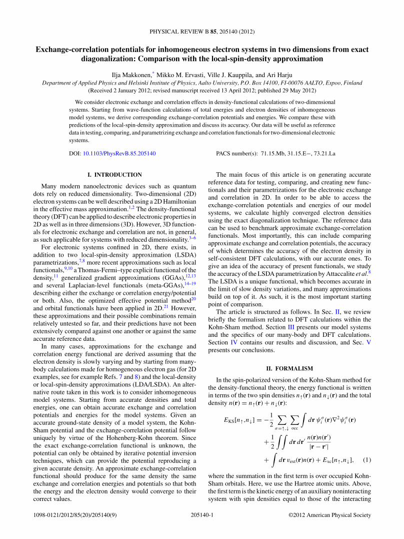
Our model systems are summarized in Table I, wherewe also list our ED total energies and DFT total energiescalculated using the LSDA parametrization by Attaccaliteet al.8 All the LSDA results in this article correspond to

1 2 3 4 5 6 7 8 9 10R (a.u.)

-0.2

-0.1

0

0.1

(EL

SD

A-E

) / |

E |

totalexchange-correlationexchangecorrelation

1 1.5 2 2.5 3 3.5

ω-1/2 (a.u.)

-0.2

-0.1

0

0.1

0.2

(EL

SD

A-E

) / |

E |

(a)

(b)

FIG. 1. (Color online) Relative errors in the LSDA energy terms(total, exchange-correlation, exchange, and correlation energies) for(a) two-electron systems in harmonic confinement and (b) twoelectrons in a hard-wall confinement as a function of the characteristiclength scale of the system 1/

√ω or R.

205140-3

MAKKONEN, ERVASTI, KAUPPILA, AND HARJU PHYSICAL REVIEW B 85, 205140 (2012)

ground-state densities of self-consistent LSDA calculations.Using ED densities and corresponding orbitals would notaffect our conclusions. The potential inversion procedureprovides us, in addition to the accurate effective potential,also with accurate Kohn-Sham orbitals. By using these and

the Kohn-Sham energy functional [Eq. (1)], we can calculatethe exact ground-state exchange-correlation energy Exc forany given model system. These, along with the correspondingapproximate LSDA values, are also listed in Table I. In thecase of the spin-singlet two-electron systems, the exchange

0

0.1

0.2

0.3

0.4

Den

sity

(H

O u

nits

)

ω = 1ω = 1/2 ω = 1/4ω = 1/10

-1.5

-1

-0.5

0

γ ×

Exc

hang

e-co

rrel

atio

n po

tent

ial (

HO

uni

ts)

0 1 2 3 4 5r (HO units)

-0.2

-0.15

-0.1

-0.05

0

γ2×

Cor

rela

tion

pot

enti

al (

HO

uni

ts)

-1.5

-1

-0.5

0

γ ×

Exc

hang

e po

tent

ial (

HO

uni

ts)

(a)

(b)

(c)

(d)

-1/r

-1/r

ω increases

ω increases

ω increases

ω increases

0

0.5

1

1.5

Den

sity

(H

W u

nits

)

-3

-2

-1

0

γ ×

Exc

hang

e-co

rrel

atio

n po

tent

ial (

HW

uni

ts)

-3

-2

-1

0

γ ×

Exc

hang

e po

tent

ial (

HW

uni

ts)

0 0.5 1r (HW units)

-0.2

-0.1

0

γ2 × C

orre

lati

on p

oten

tial

(H

W u

nits

)

(e)

(f)

(h)

(g)-1/r

-1/r

R increases

R increases

R increases

R increases

FIG. 2. (Color online) Densities (a), exchange-correlation potentials (b), exchange potentials (c), and correlation potentials (d) as a functionof the distance r for two electrons in a spin singlet in harmonic confinement ω, and (e)–(h) the same quantities for two electrons in the hard-wallconfinement with radius R. For the latter, the results for R = 2, . . . ,10 are shown. Solid lines are the accurate results and dashed lines the LSDAones. Thin dotted lines in (b), (c), (f), and (g) show the exact asymptotic −1/r behavior of the exchange potential. Natural units determined bythe external potential are used throughout.

205140-4

EXCHANGE-CORRELATION POTENTIALS FOR. . . PHYSICAL REVIEW B 85, 205140 (2012)

energy is simply28

Ex[n↑,n↓] = −1

4

∫ ∫dr dr′ n(r)n(r′)

|r − r′| , (10)

i.e., minus one-half times the Hartree energy. This allows us toeasily decompose the exchange-correlation energies of thesesystems into exchange and correlation parts.

Some ED reference results exist for the total energiesof harmonically confined systems in the literature. For thetwo-electron systems, our energies are lower than results ofRef. 29, which are 3.72143 (ω = 0.25) and 3.00097 (ω = 1).For ω = 1, there exists an analytic solution with an energyof 3 (Ref. 30). For the four-electron system with ω = 0.25,our energy is only slightly higher than one calculated byMikhailov,31 who obtained 13.6180 using a larger one-bodybasis. For six electrons with (L,S) = (0,0) and ω = 0.25,Rontani et al.32 have obtained the energy of 27.98 using 36single-particle states, which is higher than our result calculatedwith 55 states.

The ED and LSDA total energies are rather consistent forall systems, the latter one being curiously consistently higher,despite the fact that the DFT total energy is not guaranteed tobe variational once the exchange-correlation energy functionalis approximated. Similarly, the LSDA exchange-correlationenergies are higher, the exchange component being clearlyunderestimated. The lower correlation energy predicted by

the LSDA partly compensates this. This finding of errorcancellation is consistent with the results for He isoelectronicseries in 3D.23 The mechanisms behind the underestimationof the exchange energy and cancellation of errors betweenexchange and correlation energies are the same for the 2D asfor the 3D LSDA. The underestimation of exchange energyis due to self-interaction, whereas the compensating effect ofthe overestimation of the correlation energy arises from theexchange-correlation hole sum rule. Since the 2D LSDA isbased on a physical system, the 2D uniform electron gas, thesum rule is fulfilled and the integrated errors of the exchangeand correlation holes cancel.33,34

Figure 1 shows a graphical representation of LSDA’srelative errors in the total energy and the exchange-correlation,exchange and correlation energies for the two-electron systemsin harmonic and hard-wall confinements as a function ofthe characteristic length scale of the system 1/

√ω or R.

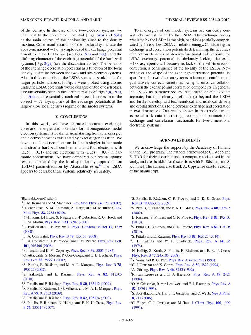
The relative errors for the total and exchange energies arerather constant as a function of the systems’ length scale.The same applies to the exchange-correlation energy, whichconsists mostly of the exchange one. The relative error in thecorrelation energy is larger at stronger confinements (largeω/small R) and becomes smaller at weaker confinement. Thisdoes not affect the overall picture much since the correlationenergy is a small fraction of the exchange-correlation one,especially at the weakly interacting (large ω/small R) limit.

0

0.1

0.2

0.3

Maj

orit

y sp

in d

ensi

ty (

HO

uni

ts)

0 0.5 1 1.5 2 2.5 3 3.5 4r (HO units)

-1.5

-1

-0.5

γ ×

Maj

orit

y sp

in x

c po

tent

ial (

HO

uni

ts)

ω = 1ω = 1/2ω = 1/4

(a)

(b)-1/r

ω increases

ω increases

0

0.1

0.2

0.3

Min

orit

y sp

in d

ensi

ty (

HO

uni

ts)

ω = 1ω = 1/2ω = 1/4

0 1 2 3 4r (HO units)

-1.5

-1

-0.5

γ ×

Min

orit

y sp

in x

c po

tent

ial (

HO

uni

ts)

(c)

(d)-1/r

ω increases

ω increases

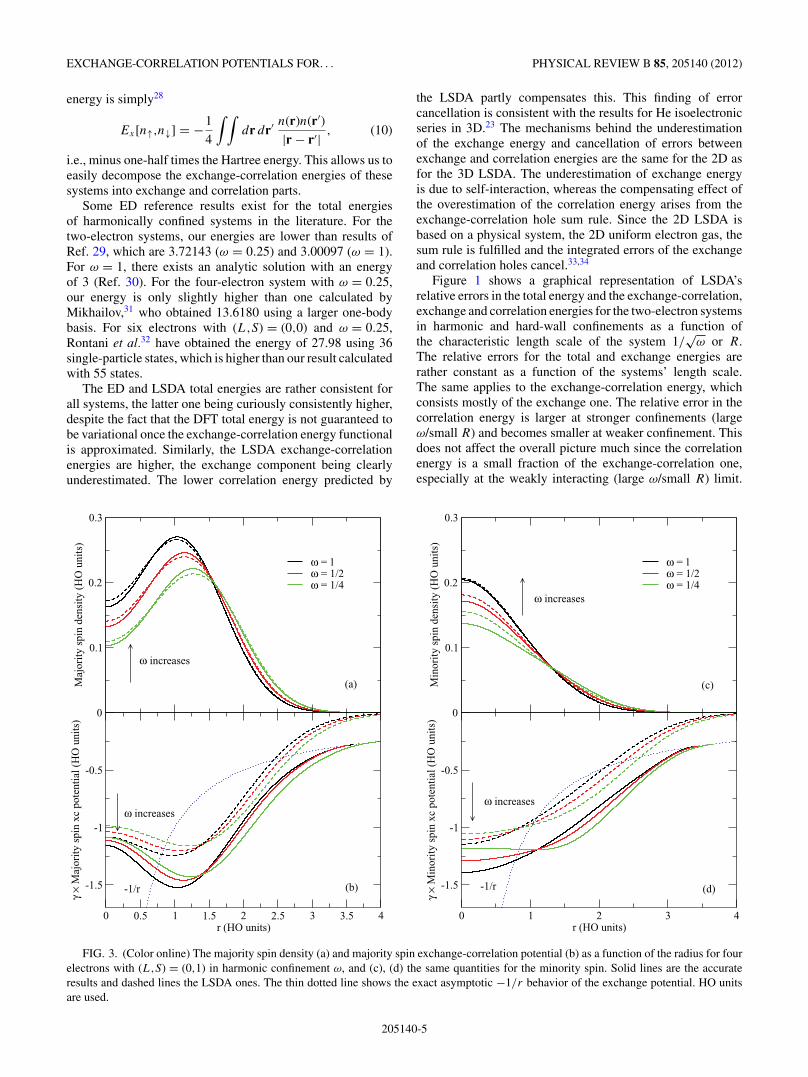
FIG. 3. (Color online) The majority spin density (a) and majority spin exchange-correlation potential (b) as a function of the radius for fourelectrons with (L,S) = (0,1) in harmonic confinement ω, and (c), (d) the same quantities for the minority spin. Solid lines are the accurateresults and dashed lines the LSDA ones. The thin dotted line shows the exact asymptotic −1/r behavior of the exchange potential. HO unitsare used.

205140-5

MAKKONEN, ERVASTI, KAUPPILA, AND HARJU PHYSICAL REVIEW B 85, 205140 (2012)

The strongly confined systems are less uniform than theircounterparts in weaker confinement. Therefore, the accuracyof the LSDA is worse in this limit. The accuracy of theLSDA energies is improved with increasing particle number.For two electrons, the level of accuracy is the same for boththe hard-wall and harmonic potentials. For four electrons, therelative error in the total energy is at most 0.6% and in theexchange-correlation energy 2.4%, and for six electrons 0.3%and 1.3%, respectively.

B. Densities and potentials

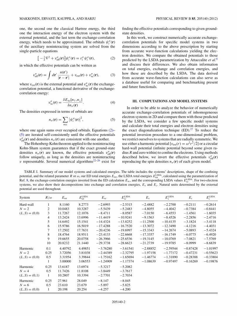
We begin the comparison of exchange-correlation po-tentials from the two-electron systems in spin singlet.Figure 2 shows electron densities and different potentialterms (exchange and correlation, exchange, correlation) for theharmonically confined electrons with varying ω and hard-wallsystems with varying R. The scaling we use when representingthe data is described and motivated below. For the two-electronsystems in spin-singlet, the exchange potential is28

vx(r) = −1

2

∫dr′ n(r′)

|r − r′| . (11)

When visualizing the potential terms, we use natural unitsand scale the exchange potential by γ and the correlationone by γ 2. Since the exchange-correlation potential consistsmostly of the exchange one, we scale it similarly. Thesescalings provide energy scales at which the potentials areof comparable magnitude and their features can be easilycompared. This can be explained using the following scalingrelations for the exchange energy35

Ex[nλ] = λEx[n], (12)

and the correlation energy36

Ec[nλ] = λ2E1/λc [n]. (13)

Above, λ is an arbitrary scaling parameter not necessarilyreferring to a transformation between two unit systems, andthe scaled density nλ is defined as

nλ(r) = λdn(λr), (14)

where d is the dimension (here 2), and E1/λc [n] is the

density functional for the correlation energy for a systemwith density n but with electron-electron interaction scaledby 1/λ. The corresponding scaling relations for the exchangeand correlation potentials are analogous. For the exchangepotential,37

vx([nλ]; r) = λvx([n]; λr), (15)

and for the correlation potential,

vc([nλ]; r) = λ2v1/λc ([n]; λr). (16)

The latter one follows from Eq. (13) similarly as Eq. (15) isderived from Eq. (12) (see Ref. 37). We apply Eqs. (15) and(16) in such a way that n corresponds to the density of a givensystem expressed in atomic units and nλ the same densityscaled to natural units (λ = γ ). Obviously, the interactionstrengths of the functionals in Eqs. (15) and (16) do not matchwith those of the above unit systems 1 and 1/γ [see Eqs. (8)

and (9)], but, nevertheless, the scaling relations motivate aconsistent visual representation.

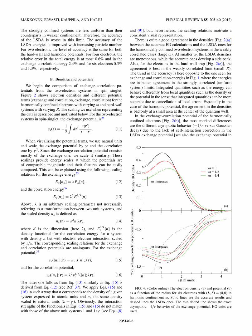
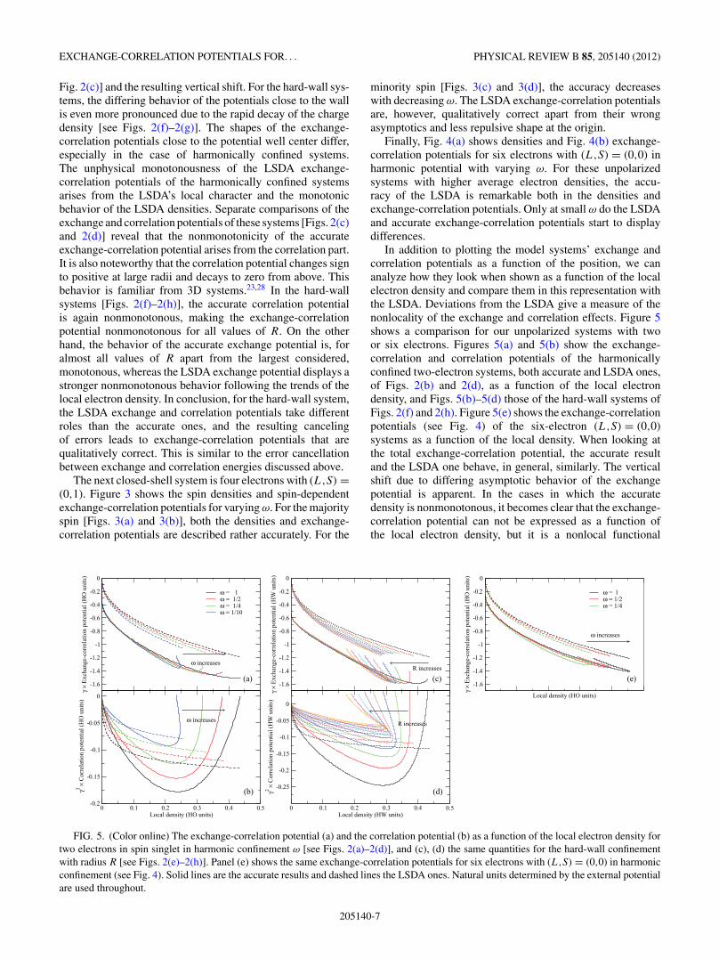
There is quite a good agreement in the densities [Fig. 2(a)]between the accurate ED calculations and the LSDA ones forthe harmonically confined two-electron systems in the weaklycorrelated cases (large ω). At smaller ω, the LSDA densitiesare monotonous, while the accurate ones develop a side peak.Also, for the electrons in the hard-wall trap [Fig. 2(e)], theagreement is best in the weakly correlated limit (small R).The trend in the accuracy is here opposite to the one seen forexchange and correlation energies in Fig. 1, where the energiesare in better agreement in the strongly correlated (uniformsystem) limits. Integrated quantities such as the energy canbehave differently from local quantities such as the density orthe potential in the sense that integrated quantities can be moreaccurate due to cancellation of local errors. Especially in thecase of the harmonic potential, the agreement in the densitiesis bad only at a small area at the center of the quantum well.

In the exchange-correlation potential of the harmonicallyconfined electrons [Fig. 2(b)], the most marked differencesare the different asymptotic behavior (−1/r versus Gaussiandecay) due to the lack of self-interaction correction in theLSDA exchange potential [see also the exchange potential in

0

0.1

0.2

0.3

0.4

0.5

Den

sity

(H

O u

nits

)

ω = 1ω = 1/2ω = 1/4

0 1 2 3 4r (HO units)

-1.5

-1

-0.5

0

γ ×

Exc

hang

e-co

rrel

atio

n po

tent

ial (

HO

uni

ts)

ω increases

ω increases

-1/r

(a)

(b)

FIG. 4. (Color online) The electron density (a) and potential (b)as a function of the radius for six electrons with (L,S) = (0,0) inharmonic confinement ω. Solid lines are the accurate results anddashed lines the LSDA ones. The thin dotted line shows the exactasymptotic −1/r behavior of the exchange potential. HO units areused.

205140-6

EXCHANGE-CORRELATION POTENTIALS FOR. . . PHYSICAL REVIEW B 85, 205140 (2012)

Fig. 2(c)] and the resulting vertical shift. For the hard-wall sys-tems, the differing behavior of the potentials close to the wallis even more pronounced due to the rapid decay of the chargedensity [see Figs. 2(f)–2(g)]. The shapes of the exchange-correlation potentials close to the potential well center differ,especially in the case of harmonically confined systems.The unphysical monotonousness of the LSDA exchange-correlation potentials of the harmonically confined systemsarises from the LSDA’s local character and the monotonicbehavior of the LSDA densities. Separate comparisons of theexchange and correlation potentials of these systems [Figs. 2(c)and 2(d)] reveal that the nonmonotonicity of the accurateexchange-correlation potential arises from the correlation part.It is also noteworthy that the correlation potential changes signto positive at large radii and decays to zero from above. Thisbehavior is familiar from 3D systems.23,28 In the hard-wallsystems [Figs. 2(f)–2(h)], the accurate correlation potentialis again nonmonotonous, making the exchange-correlationpotential nonmonotonous for all values of R. On the otherhand, the behavior of the accurate exchange potential is, foralmost all values of R apart from the largest considered,monotonous, whereas the LSDA exchange potential displays astronger nonmonotonous behavior following the trends of thelocal electron density. In conclusion, for the hard-wall system,the LSDA exchange and correlation potentials take differentroles than the accurate ones, and the resulting cancelingof errors leads to exchange-correlation potentials that arequalitatively correct. This is similar to the error cancellationbetween exchange and correlation energies discussed above.

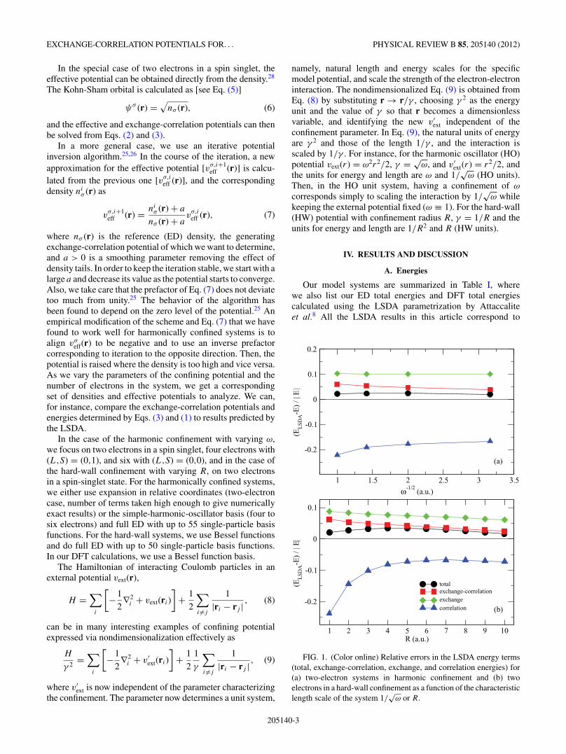
The next closed-shell system is four electrons with (L,S) =(0,1). Figure 3 shows the spin densities and spin-dependentexchange-correlation potentials for varying ω. For the majorityspin [Figs. 3(a) and 3(b)], both the densities and exchange-correlation potentials are described rather accurately. For the

minority spin [Figs. 3(c) and 3(d)], the accuracy decreaseswith decreasing ω. The LSDA exchange-correlation potentialsare, however, qualitatively correct apart from their wrongasymptotics and less repulsive shape at the origin.

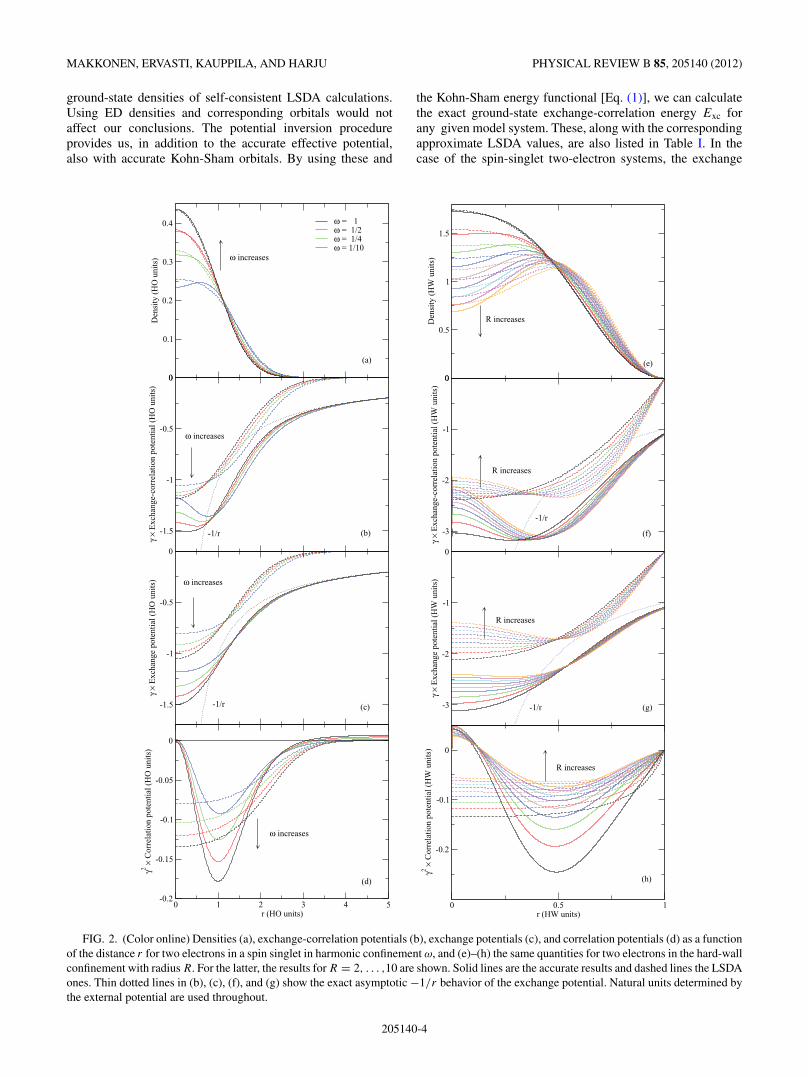
Finally, Fig. 4(a) shows densities and Fig. 4(b) exchange-correlation potentials for six electrons with (L,S) = (0,0) inharmonic potential with varying ω. For these unpolarizedsystems with higher average electron densities, the accu-racy of the LSDA is remarkable both in the densities andexchange-correlation potentials. Only at small ω do the LSDAand accurate exchange-correlation potentials start to displaydifferences.

In addition to plotting the model systems’ exchange andcorrelation potentials as a function of the position, we cananalyze how they look when shown as a function of the localelectron density and compare them in this representation withthe LSDA. Deviations from the LSDA give a measure of thenonlocality of the exchange and correlation effects. Figure 5shows a comparison for our unpolarized systems with twoor six electrons. Figures 5(a) and 5(b) show the exchange-correlation and correlation potentials of the harmonicallyconfined two-electron systems, both accurate and LSDA ones,of Figs. 2(b) and 2(d), as a function of the local electrondensity, and Figs. 5(b)–5(d) those of the hard-wall systems ofFigs. 2(f) and 2(h). Figure 5(e) shows the exchange-correlationpotentials (see Fig. 4) of the six-electron (L,S) = (0,0)systems as a function of the local density. When looking atthe total exchange-correlation potential, the accurate resultand the LSDA one behave, in general, similarly. The verticalshift due to differing asymptotic behavior of the exchangepotential is apparent. In the cases in which the accuratedensity is nonmonotonous, it becomes clear that the exchange-correlation potential can not be expressed as a function ofthe local electron density, but it is a nonlocal functional

-1.6

-1.4

-1.2

-1

-0.8

-0.6

-0.4

-0.2

0

γ ×

Exc

hang

e-co

rrel

atio

n po

tent

ial (

HO

uni

ts)

ω = 1ω = 1/2ω = 1/4ω = 1/10

0 0.1 0.2 0.3 0.4 0.5Local density (HO units)

-0.2

-0.15

-0.1

-0.05

0

γ2 × C

orre

lati

on p

oten

tial

(H

O u

nits

)

(a)

(b)

ω increases

ω increases

-1.6

-1.4

-1.2

-1

-0.8

-0.6

-0.4

-0.2

0

γ ×

Exc

hang

e-co

rrel

atio

n po

tent

ial (

HW

uni

ts)

0 0.1 0.2 0.3 0.4 0.5Local density (HW units)

-0.25

-0.2

-0.15

-0.1

-0.05

0

γ2 × C

orre

lati

on p

oten

tial

(H

W u

nits

)

(c)

(d)

R increases

R increases

Local density (HO units)

-1.6

-1.4

-1.2

-1

-0.8

-0.6

-0.4

-0.2

0

γ ×

Exc

hang

e-co

rrel

atio

n po

tent

ial (

HO

uni

ts)

ω = 1ω = 1/2ω = 1/4

ω increases

(e)

FIG. 5. (Color online) The exchange-correlation potential (a) and the correlation potential (b) as a function of the local electron density fortwo electrons in spin singlet in harmonic confinement ω [see Figs. 2(a)–2(d)], and (c), (d) the same quantities for the hard-wall confinementwith radius R [see Figs. 2(e)–2(h)]. Panel (e) shows the same exchange-correlation potentials for six electrons with (L,S) = (0,0) in harmonicconfinement (see Fig. 4). Solid lines are the accurate results and dashed lines the LSDA ones. Natural units determined by the external potentialare used throughout.

205140-7

MAKKONEN, ERVASTI, KAUPPILA, AND HARJU PHYSICAL REVIEW B 85, 205140 (2012)

of the density. In the case of the two-electron systems, wecan identify the correlation potential [Figs. 5(b) and 5(d)]as the main source of the nonlocality close to the densitymaxima. Other manifestations of the nonlocality include theabove-mentioned −1/r asymptotics of the exchange potentialabsent from the LSDA one [see Figs. 2(c) and 2(g)], and thediffering character of the exchange potential of the hard-wallsystems [Fig. 2(g)] (see the discussion above). The behaviorof the exchange-correlation potential as a function of the localdensity is similar between the two- and six-electron systems.Also in this comparison, the LSDA seems to work better forlarger particle numbers. If Fig. 5 were plotted using atomicunits, the LSDA potentials would collapse on top of each other.The universality seen in the accurate results of Figs 5(a), 5(c),and 5(e) is an essentially nonlocal effect. It arises from thecorrect −1/r asymptotics of the exchange potentials at thelarge-r (low local density) regime of the model systems.

V. CONCLUSIONS

In this work, we have extracted accurate exchange-correlation energies and potentials for inhomogeneous modelelectron systems in two dimensions starting from total energiesand electron densities calculated by exact diagonalization. Wehave considered two electrons in a spin singlet in harmonicand circular hard-wall confinements and four electrons with(L,S) = (0,1) and six electrons with (L,S) = (0,0) in har-monic confinement. We have compared our results againstresults calculated by the local-spin-density approximation(LSDA) parametrization by Attaccalite et al.8 The LSDAappears to describe these systems relatively accurately.

Total energies of our model systems are curiously con-sistently overestimated by the LSDA. The exchange energypredicted by the LSDA is too high, but this is partially compen-sated by the too-low LSDA correlation energy. Considering theexchange and correlation potentials determining the accuracyof electron densities in density-functional calculations, theLSDA exchange potential is obviously lacking the exact−1/r asymptotic tail because its lack of the self-interactioncorrection, a consequence of the locality of the LSDA. Nev-ertheless, the shape of the exchange-correlation potential is,apart from the two-electron systems in harmonic confinement,qualitatively correct, sometimes owing to error cancellationbetween the exchange and correlation components. In general,the LSDA as parametrized by Attaccalite et al.8 is quiteaccurate, but it is clearly useful to go beyond the LSDAand further develop and test semilocal and nonlocal densityand orbital functionals for electronic exchange and correlationin two dimensions. Our results shown in this article can actas benchmark data in creating, testing, and parametrizingexchange and correlation functionals for two-dimensionalelectronic systems.

ACKNOWLEDGMENTS

We acknowledge the support by the Academy of Finlandvia the CoE program. The authors acknowledge C. Webb andE. Tolo for their contributions to computer codes used in thestudy, and are thankful for discussions with E. Rasanen and S.Kummel. The authors also thank A. Uppstu for careful readingof the manuscript.

*ilja.makkonen@aalto.fi1S. M. Reimann and M. Manninen, Rev. Mod. Phys. 74, 1283 (2002).2H. Saarikoski, S. M. Reimann, A. Harju, and M. Manninen, Rev.Mod. Phys. 82, 2785 (2010).

3Y.-H. Kim, I.-H. Lee, S. Nagaraja, J.-P. Leburton, R. Q. Hood, andR. M. Martin, Phys. Rev. B 61, 5202 (2000).

4L. Pollack and J. P. Perdew, J. Phys.: Condens. Matter 12, 1239(2000).

5L. A. Constantin, Phys. Rev. B 78, 155106 (2008).6L. A. Constantin, J. P. Perdew, and J. M. Pitarke, Phys. Rev. Lett.101, 016406 (2008).

7B. Tanatar and D. M. Ceperley, Phys. Rev. B 39, 5005 (1989).8C. Attaccalite, S. Moroni, P. Gori-Giorgi, and G. B. Bachelet, Phys.Rev. Lett. 88, 256601 (2002).

9S. Pittalis, E. Rasanen, and M. A. L. Marques, Phys. Rev. B 78,195322 (2008).

10S. Sakiroglu and E. Rasanen, Phys. Rev. A 82, 012505(2010).

11S. Pittalis and E. Rasanen, Phys. Rev. B 80, 165112 (2009).12S. Pittalis, E. Rasanen, J. G. Vilhena, and M. A. L. Marques, Phys.

Rev. A 79, 012503 (2009).13S. Pittalis and E. Rasanen, Phys. Rev. B 82, 195124 (2010).14S. Pittalis, E. Rasanen, N. Helbig, and E. K. U. Gross, Phys. Rev.

B 76, 235314 (2007).

15S. Pittalis, E. Rasanen, C. R. Proetto, and E. K. U. Gross, Phys.Rev. B 79, 085316 (2009).

16S. Pittalis, E. Rasanen, and E. K. U. Gross, Phys. Rev. A 80, 032515(2009).

17E. Rasanen, S. Pittalis, and C. R. Proetto, Phys. Rev. B 81, 195103(2010).

18S. Pittalis, E. Rasanen, and C. R. Proetto, Phys. Rev. B 81, 115108(2010).

19S. Pittalis and E. Rasanen, Phys. Rev. B 82, 165123 (2010).20J. D. Talman and W. F. Shadwick, Phys. Rev. A 14, 36

(1976).21N. Helbig, S. Kurth, S. Pittalis, E. Rasanen, and E. K. U. Gross,

Phys. Rev. B 77, 245106 (2008).22Y. Wang and R. G. Parr, Phys. Rev. A 47, R1591 (1993).23C. J. Umrigar and X. Gonze, Phys. Rev. A 50, 3827 (1994).24A. Gorling, Phys. Rev. A 46, 3753 (1992).25R. van Leeuwen and E. J. Baerends, Phys. Rev. A 49, 2421

(1994).26O. V. Gritsenko, R. van Leeuwen, and E. J. Baerends, Phys. Rev. A

52, 1870 (1995).27S. S. Gylfadottir, A. Harju, T. Jouttenus, and C. Webb, New J. Phys.

8, 211 (2006).28C. Filippi, C. J. Umrigar, and M. Taut, J. Chem. Phys. 100, 1290

(1994).

205140-8

EXCHANGE-CORRELATION POTENTIALS FOR. . . PHYSICAL REVIEW B 85, 205140 (2012)

29O. Ciftja and M. G. Faruk, Phys. Rev. B 72, 205334 (2005).30M. Taut, J. Phys. A: Math. Gen. 27, 1045 (1994).31S. A. Mikhailov, Phys. Rev. B 66, 153313 (2002).32M. Rontani, C. Cavazzoni, D. Bellucci, and G. Goldoni, J. Chem.

Phys. 124, 124102 (2006).33O. Gunnarsson, M. Jonson, and B. I. Lundqvist, Phys. Rev. B 20,

3136 (1979).

34R. Q. Hood, M. Y. Chou, A. J. Williamson, G. Rajagopal, and R. J.Needs, Phys. Rev. B 57, 8972 (1998).

35M. Levy and J. P. Perdew, Phys. Rev. A 32, 2010 (1985).36M. Levy, in Single-Particle Density in Physics and Chemistry,

edited by N. H. March and B. M. Deb (Academic, London, 1987),p. 45.

37H. Ou-Yang and M. Levy, Phys. Rev. Lett. 65, 1036 (1990).

205140-9