mainvol1 - UNAM

Chapter 18

Topics of FunctionalAnalysis

In Chapter 14 there have been introduced the important concepts suchas

1) Lineality of a space of elements,

2) Metric (or norm) in a space,

3) Compactness, convergence of a sequence of elements and Cauchysequences,

4) Contraction principle.

As the examples we have considered in details the finite dimensionalspaces R and C of real and complex vectors (numbers). But thesame definitions of lineality and norms remain true if we consider asanother example a functional space (where an element is a function)or a space of sequences (where an element is a sequence of real orcomplex vectors). The specific feature of such spaces is that all ofthem are infinite dimensional. This chapter deals with the analysis ofsuch spaces which is called "Functional Analysis".Let us introduce two important additional concept which will be

use below.

Definition 18.1 The subset V of a linear normed space X is said tobe dense in X if its closure is equal to X .

507

508 Chapter 18. Topics of Functional Analysis

This property means that every element X may be approx-imated as closely as we like by some element V, that is, forany X and any 0 there exists an element V such thatk k .All normed linear spaces have dense subsets, but they need not be

obligatory countable subsets.

Definition 18.2 A normed linear space X is said to be separable ifit contains at least one dense subset which is countable.

The separable spaces have special properties that are importantin di erent applications. In particular, denoting the elements of suchcountable subset by { } =1 it is possible to represent each element

X as the convergent series

=P=1

(18.1a)

where the scalars R are called the coordinates of the elementin the basis { } =1 .

18.1 Linear and normed spaces of func-tions

Below we will introduce the examples of some functional spaces withthe corresponding norm within. The lineality and main properties ofa norm (metric) can be easily verified that’s why we leave this for areader as an exercise.

18.1.1 Space of all bounded complex numbers

Let us consider a set of sequences := { } =1 such thatC and sup k k (18.2)

where k k :=rP

=1

¯ and introduce the norm in as

k k := sup k k (18.3)

18.1. Linear and normed spaces of functions 509

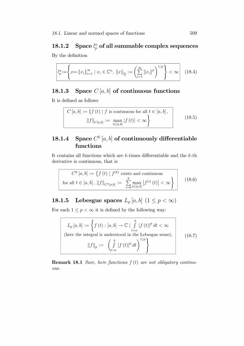
18.1.2 Space of all summable complex sequences

By the definition

:=

(={ } =1 | C k k :=

μP=1

k k¶1 )

(18.4)

18.1.3 Space [ ] of continuous functions

It is defined as follows

[ ] := { ( ) | is continuous for all [ ]

k k [ ] := max[ ]| ( )|

¾(18.5)

18.1.4 Space [ ] of continuously di erentiablefunctions

It contains all functions which are -times di erentiable and the -thderivative is continuous, that is

[ ] :=©( ) | ( ) exists and continuous

for all [ ] k k [ ] :=P=0

max[ ]

¯̄( ) ( )

¯̄ ¾(18.6)

18.1.5 Lebesgue spaces [ ] (1 )

For each 1 it is defined by the following way:

[ ] :=

½( ) : [ ] C | R

=

| ( )|(here the integral is understood in the Lebesgue sense),

k k :=

μ R=

| ( )|¶1 ) (18.7)

Remark 18.1 Sure, here functions ( ) are not obligatory continu-ous.


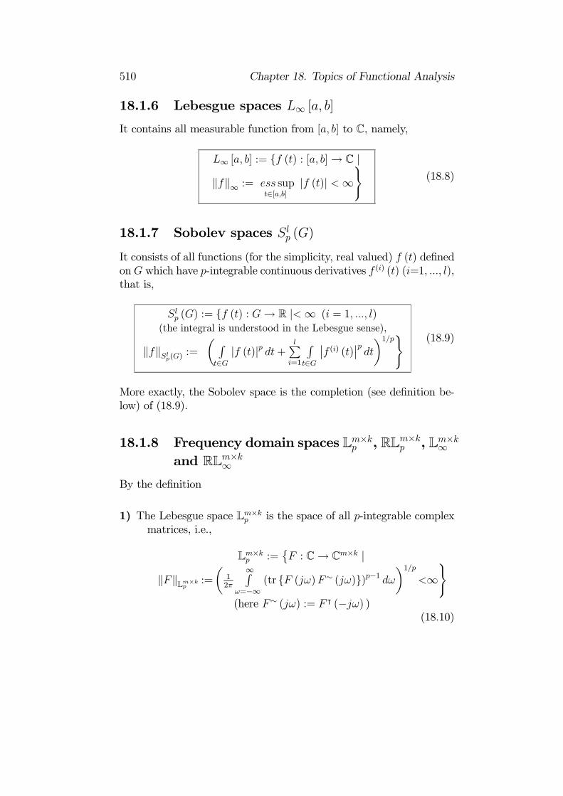
18.1.6 Lebesgue spaces [ ]

It contains all measurable function from [ ] to C, namely,

[ ] := { ( ) : [ ] C |k k := sup

[ ]

| ( )|)

(18.8)

18.1.7 Sobolev spaces ( )

It consists of all functions (for the simplicity, real valued) ( ) definedon which have -integrable continuous derivatives ( ) ( ) ( =1 ),that is,

( ) := { ( ) : R | ( = 1 )(the integral is understood in the Lebesgue sense),

k k ( ) :=

μ R | ( )| +P=1

R ¯̄( ) ( )

¯̄ ¶1 ) (18.9)

More exactly, the Sobolev space is the completion (see definition be-low) of (18.9).

18.1.8 Frequency domain spaces L × , RL × , L ×

and RL ×

By the definition

1) The Lebesgue space L × is the space of all -integrable complexmatrices, i.e.,

L × :=©

: C C × |k k

L× :=

μ12

R=

(tr { ( ) ( )}) 1

¶1 )

(here ( ) := | ( ) )(18.10)

18.1. Linear and normed spaces of functions 511

2) The Lebesgue space RL × is the subspace of L × containingonly complex matrices with rational elements, i.e., in

= k ( )k =1 ; =1

each element ( ) represents the polynomial ratio

( ) =0 + 1 + +0 + 1 + +

and are positive integer(18.11)

Remark 18.2 If for each element of , then ( )can be interpreted as a matrix transfer function of a linear(finite-dimensional) system.

3) The Lebesgue space L × is the space of all complex matrices withbounded (almost everywhere) on the imaginary axis elements,i.e.

L× :=

©: C C

× |k k

L× := sup

:Re 0

1 2max { ( ) ( )}

¾= sup

( )

1 2max { ( ) ( )}

(18.12)

(the last equality may be regarded to as a the generalization ofthe Maximum Modulus Principle 17.10 for matrix functions).

4) The Lebesgue space RL × is the subspace of L × containingonly complex matrices with rational elements given in the form(18.11).

18.1.9 Hardy spacesH × , RH × , H × and RH ×

The Hardy spaces H × , RH × , H × and RH × are subspaces ofthe corresponding Lebesgue spaces L × , RL × , L × and RL ×

containing complex matrices with only regular (holomorphic) (see De-finition 17.2) elements on the open half-plane Re 0.


Remark 18.3 If for each element of , then ( )RH

× can be interpreted as a matrix transfer function of astable linear (finite-dimensional) system.

Example 18.1

1

2RL2 := RL

1×12

1

2RL := RL1×1

1

2 +HL2 := HL

1×12

1

2 +RH := RH1×1

2L2 := L

1×12 2 +

H2 := H1×12

1

2L := L1×1

1

2 +H := H1×1

18.2 Banach spaces

18.2.1 Basic definition

Remember that a linear normed (topological) space X is said to becomplete (see Definition 14.14) if every Cauchy (fundamental) se-quence has a limit in the same space X . The concept of a completespace is very import since even without evaluating the limit one candetermine whether a sequence is convergent or not. So, if a metric(topological) space is not a complete it is impossible talk about aconvergence, limits, di erentiation and so on.

Definition 18.3 A linear, normed and complete space is called a Ba-nach space.

18.2.2 Examples of incomplete metric spaces

Sure that not all linear normed (metric) spaces are complete. Theexample given below illustrates this fact.

Example 18.2 (of a noncomplete normed space) Let us considerthe space [0 1] of all continuous functions : [0 1] which are

18.2. Banach spaces 513

absolutely integrable (in this case, in the Riemann sense) on [0 1], thatis, for which

k k [0 1] :=

1Z= 1

| ( )| (18.13)

Consider the sequence { } of the continuous functions

:=

½if [0 1 ]

1 if [1 1]

Then for

k k [0 1] =1R=0

| ( ) ( )| =

1R=0

| | +1R=1

|1 | +1R

=1

|1 1|( )

2 2+(1 )2

2=1

2

μ1 1

¶0

as . So, { } is a Cauchy sequence. However, its pointwiselimit is

( )

½1 if 0 10 if = 0

In other words, the limit is a discontinuous function and, hence, it isnot in [0 1]. This means that the functional space [0 1] is notcomplete.

Example 18.3 By the same reason, the spaces [0 1] (the spaceof continuous and -integrable functions) are not complete.

18.2.3 Completion of metric spaces

There exist two possibilities to correct the situation and to providethe completeness property for a linear normed space if initially bit isnot a complete:

• try to change the definition of a norm;• try to extend the class of considered functions (it was suggestedby Cauchy).


Changing of a norm

To illustrate the first approach related to changing of a norm let usconsider again the space of all functions continuous at the interval[0 1], but instead of the Lebesgue norm (18.13) we consider the Cheby-shev’s type norm k k [ ] as in (18.5). This means that instead of thespace [0 1] we will consider the space [ ] (18.5). Evidently,that this space is complete, since it is known that uniform convergentsequences of continuous functions converges to a continuous function.Hence, [ ] is a Banach space under this norm.

Claim 18.1 By the same reasons it is not di cult to show that allspaces [ ] (18.6) are Banach.

Claim 18.2 The spaces [ ] (1 ) (18.7), [ ] (18.8),L

× , (23.19) and L × (18.12) are Banach too.

Completion

Theorem 18.1 Any linear normed space X with a norm k kX canbe considered as a linear manifold which is complete in some Banachspace X̂ . This space X̂ is called the completion of X .Proof. Consider two fundamental sequences { } and { 0 } with

elements from X . We say that they are equivalent if k 0 k 0as and we will write { } { 0 }. The set of all fundamentalsequences may be separated (factorized) at non crossed classes: { }and { 0 } are included in the same class if and only if { } { 0 }.The set of all such classes X we denoted by X̂ . So,

X̂ :=[X X

6=X =

Let us make the space X̂ a normed space. To do that, define theoperation of summing of the classes X by the following manner: if{ } X and { } X then class (X + X ) may be defined as theclass containing { + }. The operation of the multiplication by aconstant may be introduced as follows: we denoted by X the classcontaining { } if { } X . It is evident that X̂ is a linear space.Define now the norm in X̂ as

kX k := lim k kX ({ } X )

18.3. Hilbert spaces 515

It easy to check the norm axioms for such norm and to show that

a) X may be considered as a linear manifold in X̂ ;b) X is dense in X̂ , i.e., there exists { } X such that k X kX

0 as as for some X X ;c) X̂ is complete (Banach).

This complete the proof.This theorem can be interpreted as the following statement.

Corollary 18.1 For any linear norm space X there exists a Banachspace X̂ and a linear, injective map : X X̂ such that (X ) isdense in X̂ and for all X

k kX̂ = k kX

18.3 Hilbert spaces

18.3.1 Definition and examples

Definition 18.4 A Hilbert space H is an inner (scalar) productspace that is complete as a linear normed space under the inducednorm

k kH :=ph i (18.14)

Example 18.4 The following spaces are Hilbert

1. The space 2 of all summable complex sequences (see (18.4)for = 2) under the inner product

h i2:=P=1

¯ (18.15)

2. The Lebesgue space 2 [ ] of all integrable (in Lebesgue sense)complex functions (see (18.7) for = 2) under the inner product

h i2[ ] :=

R=

( )¯( ) (18.16)


3. The Sobolev’s space 2 ( ) of all times di erentiable onquadratically integrable (in Lebesgue sense) complex functions(see (18.9) for = 2) under the inner product

h i ( ) :=P=0

¿ À2[ ]

(18.17)

4. The frequency domain space L ×2 of all -integrable complex

matrices (23.19) under the inner product

h iL

× :=R=

tr{ ( ) ( )} (18.18)

5. TheHardy spaces H ×2 (the subspace of L ×

2 containing onlyholomorphic in the right-hand semi-plan C+ := { C |Re 0}functions) under the inner product (18.18).

18.3.2 Orthogonal complement

Definition 18.5 LetM be a subset of a Hilbert space H, i.e.,MH. Then the distance between a point H andM is defined by

( M) := infMk k (18.19)

The following claim seems to be evident.

Claim 18.3 If M, then ( M) = 0. If M andM is closedset (see Definition 14.7), then ( M) 0.

Corollary 18.2 If M H is closed convex set and M, thenthere exists a unique element M such that ( M) = k k.

Proof. Indeed, suppose that there exists another element Msuch that

( M) = k k = k k :=


Then

4 2 = 2 k k2 + 2 k k2 = k k2+4

°°°° +

2

°°°°2

k k2 + 4 infMk k2

k k2 + 4 2

that gives k k2 0, or equivalently, = .

Corollary 18.3 IfM H is a subspace of H (this means that it isclosed convex linear manifold in H) then for any H there exists aunique element M M such that

( M) := infMk k = k Mk (18.20)

This element M M is called the orthogonal projection of theelement H onto the subspaceM H.Lemma 18.1 Let ( M) = k Mk whereM is a subspace of aHilbert space H with the inner product h iH. Then ( M) M,that is, for any M

h M iH = 0 (18.21)

Proof. By the definition (18.20) for any C (here M +M) we have

k ( M + )k k Mkthat implies

h M iH + ¯ h MiH + ¯ k k2 0

Taking =h M iH

k k2 one has|h M i|2

k k2 0 that leads

to the equality h M iH = 0. Lemma is proven.Definition 18.6 If M is a subspace of a Hilbert space H then theorthogonal complementM is defined by

M := { H | h iH = 0 for all M} (18.22)


It is easy to show thatM is a closed linear subspace of and thatH can be uniquely decomposed as the direct sum

H = M̄ M (18.23)

This means that any element H has the unique representation

= M̄ + M (18.24)

where M M̄ and M M such that k k2 = k Mk2 + k M k2.Theorem 18.2 Let If M is a subspace of a Hilbert space H. M isdense in H if and only ifM = {0}.Proof. a) Necessity. Let M is dense in H. This means that

M̄ = H. Assume that there exists 0 H such that 0 M. Let{ } M and H. Then 0 = h 0i h 0i = 0 sinceM is dense in H. Taking = 0 we get that h 0 0i = 0 that gives0 = 0. b) Su ciency. LetM = {0}, that is, if h 0i = 0 for anyM, then 0 = 0. Suppose thatM is not dense in H. This means

that there exists 0 M̄. Then by the orthogonal decomposition

0 = 0 + 0 where 0 M̄ and 0

¡M̄¢=M . Here 0 6= 0 for

which h 0 iH = 0 for any M̄. By the assumption such element0 = 0. We get the contradiction. Theorem is proven.

18.3.3 Fourier series in Hilbert spaces

Definition 18.7 An orthonormal system (set) { } of functionsin a Hilbert space H is a nonempty subset { | 1} of H such that

h iH = =

½1 if =0 if 6= (18.25)

1. The seriesP=1

is called the series in H with respect of the

system { } (18.25);2. For any H the representation (if it exists)

( ) =P=1

( ) (18.26)

is called the Fourier expansion of with respect to { }.


Lemma 18.2 In (18.26)

= h iH (18.27)

Proof. Premultiplying (18.26) by and using (18.25) we find

h iH =X=1

h iH =X=1

=

that proves (18.27). Lemma is proven.

Corollary 18.4 (the Parseval equality)

k k2 = P=1

|h iH|2 (18.28)

Proof. It follows from the relation

h iH =P=1

P=1

h iH h iH h iH =P=1

P=1

h iH h iH =P=1

|h iH|2

Example 18.5

1) Classical Fourier expansion. In H = 2 [0 1] the corre-sponding orthogonal basis { } is

{ } = ©1 2 sin (2 ) 2 cos (2 ) 1ª

that implies

( ) = 0 + 2X=1

sin (2 ) + 2X=1

cos (2 )

where

0 =1R=0

( ) =1R=0

( ) 2 cos (2 )

=1R=0

( ) 2 sin (2 )


2) Legandre expansion. In H = 2 [0 1] the corresponding or-thogonal basis { } is { } = { } where

:=1

2 !

h( 2 1)

i1

18.3.4 Linear -manifold approximation

Definition 18.8 The collection of the elements

:=P=1

H C ( 1) (18.29)

is called the linear -manifold generated by the system of functions{ } =1 .

Theorem 18.3 The best 2-approximation of any elements Hby the element from the -manifold (18.29) is given by the Fouriercoe cients = (18.27), namely,

inf: =1

°°°° P=1

°°°°2

2

=

°°°° P=1

°°°°2

2

(18.30)

Proof. It follows from the identity

k k22=

°°°° P=1

°°°°2

2

=°°°°P=1

( )P=1

°°°°2

2

=

P= +1

| |2 k k22+P=1

| |2 k k22

that reaches the minimum if =¡

: = 1¢. Theorem is

proven.

18.4. Linear operators and functionals in Banach spaces 521

18.4 Linear operators and functionals inBanach spaces

18.4.1 Operators and functionals

Definition 18.9

1. Let X and Y be be linear normed spaces (usually, either Banachor Hilbert spaces) and : D Y be a transformation (oroperator) from a subset D X to Y. D = D ( ) is called thedomain (image) of the operator and values (D) constitutethe range (the set of possible values) R ( ) of . If the range ofthe operator is finite-dimensional the we say that the operatorhas the finite range.

2. If Y is a scalar field F (usually R) then the transformationsare called functionals.

3. A functional is linear if it is additive, i.e., for any D

( + ) = +

and homogeneous, i.e., for any D and any F

( ) =

4. Operators for which the domain D and the range (D) are inone-to-one correspondence are called invertible. The inverseoperator is denoted by 1 : (D) D, so that

D 1 ( (D))

Example 18.6

1. The shift operator : defined by

= +1

for any = 1 2 .


2. The integral operator : 2 [ ] R defined by

:=R=

( ) ( )

for any 2 [ ].

3. The di erential operator : D ( ) = 1 [ ] [ ]defined by

:= ( )

for any 1 [ ] and any [ ].

It is evident the following statement.

Claim 18.4

1. is invertible if and only if it is injective, that is, = 0implies = 0. The set { D | = 0} is called the kernel ofthe operator and denoted by

ker := { D | = 0}

So, is injective if and only if ker = {0}.2. If is linear and invertible then 1 is also linear.

18.4.2 Continuity and boundedness

Continuity

Definition 18.10

1. Let : D ( ) Y be a map (operator) between two linearnormed spaces X (with a norm k·kX ) and Y (with a norm k·kY).It is said to be a continuous at 0 X if, given 0, thereexists a = ( ) 0 such that k ( ) ( 0)kY , wheneverk 0kX .


2. is semi-continuous at a point 0 X if it transforms anyconvergent sequence { } D ( ), 0, in to asequence { ( )} R ( ) weakly convergent to ( 0), i.e.,k ( ) ( 0)k 0 when .

3. is continuous (or semi-continuous) on D ( ) if it is con-tinuous (or semi-continuous) at every point in D ( ).

Lemma 18.3 Let X and Y be Banach spaces and be a linear op-erator defined at X . If is continuous at the point 0 X , thenis continuous at any point 0 X .

Proof. This result follows from the identity 0 = ( 0).If 0, then := 0 0. By continuity at zero 0 thatimplies 0 0. Lemma is proven.So, a linear operator may be called continuous, if it is continuous

at the point 0 = 0.

Boundedness

Definition 18.11

1. A linear operator : D ( ) X Y between two linear normedspaces X (with a norm k·kX ) and Y (with a norm k·kY) is saidto be bounded if there exists a real number 0 such that forall D ( )

k kY k kX (18.31)

The set of all bounded linear operators : D ( ) X Yis usually denoted by L (X Y).

2. A linear operator : D ( ) X Y is called a compactoperator if it maps any bounded subset of X onto a compact setof Y.

3. The induced norm of a linear bounded operator : D ( )X Y may be introduced as follows

k k := supD( ) 6=0

k kYk kX

= supD( ) k kX=1

k kY (18.32)


(here it is assumed that if D ( ) = {0} then by the definitionk k = 0 since 0 = 0).

It seems to be evident that the continuity and boundedness forlinear operators are equivalent concepts.

Claim 18.5 A linear operator : D ( ) X Y is continuous ifand only if it is bounded.

Example 18.7

1. If :=

Ã P=1

| |!1

( 1), then the "weighting"

operator defined by

= :=P=1

(18.33)

making from to ( 1 + 1 = 1) is linear and bounded sinceby the Hölder inequality (16.134)

k k =P=1

¯̄̄¯̄P=1

¯̄̄¯̄ P

=1

ÃP=1

| |!ÃP

=1

| |!

=

ÃP=1

| |!

= k k

2. If :=R=

R=

| ( )| , then the integral operator

: X = [ ] Y = [ ] = Y ( 1 + 1 = 1) definedby

= :=R=

( ) ( ) (18.34)

is linear and bounded since by the Hölder inequality (16.134)

k k [ ] :=R=

¯̄̄¯ R=

( ) ( )

¯̄̄¯

R=

μ R=

| ( )|¶μ R

=

| ( )|¶

= k k [ ]


3. If := maxD̄

P=0

| ( )| , then the di erential operator

: D X = [ ] Y = [ ] = Y defined by

= :=P=0

( ) ( ) ( ) (18.35)

is linear and bounded since

k k [ ] := maxD̄

¯̄̄¯P=0

( ) ( ) ( )

¯̄̄¯

maxD̄

μP=0

| ( )|P=0

¯̄( ) ( )

¯̄¶ k k [ ]

Sequence of linear operators and uniform convergence

It is possible to introduce several di erent notions of a convergence inthe space of linear bounded operators L (X Y) acting from X to Y.

Definition 18.12 Let { } L (X Y) be a sequence of operators.

1. We say that

- uniformly converges to L (X Y) if k k 0whenever . Here the norm k k is understood as in(18.32);

- strongly converges to L (X Y) if k kY 0whenever for any X .

2. If the operator is dependent on the parameter A, then- ( ) is uniformly continuous at 0 A, if

k ( ) ( 0)k 0 as 0

- ( ) is strongly continuous at 0 A, if for all X

k ( ) ( 0) kY 0 as 0

In view of this definition the following claim seems to be evident.


Claim 18.6 uniformly converges to L (X Y) if and only ifuniformly on X in the ball k kX 1.

Theorem 18.4 If X is a linear normed space and Y is a Banachspace, then L (X Y) is a Banach space too.

Proof. Let { } be a fundamental sequence in the metric ofL (X Y), that is, for any 0 there exists a number 0 = 0 ( )such that for any 0 and any natural we have k + k .Then the sequence { } is also fundamental. But Y is complete,and hence, { } converges. Denote := lim . By this formula

any element X is mapped into an element of Y, and, hence, itdefines the operator = . Let us prove that the linear operator isbounded (continuous). First, notice that {k k} is also fundamental.This follows from the inequality |k + k k k| k + k.But it means that {k k} is bounded, that is, there exists 0 suchthat k k for every 1. Hence, k k k k. Taking thelimit in the right-hand side we obtain k k k k that shows thatis bounded. Theorem is proven.

Extension of linear bounded operators

Bounded linear operators that map into a Banach space always havea unique extension to the closure of their domain without changing ofits norm value.

Theorem 18.5 Let : D ( ) X Y be a linear bounded operator(functional) mapping the linear normed space X into a Banach spaceY. Then it has a unique bounded extension ˜ : D ( ) Y such that

1. ˜ = for any D ( ) ;

2.°°° ˜°°° = k k.

Proof. If D ( ), put ˜ = . Let X , but D ( ).By the density of D ( ) in X , there exists the sequence { } D ( )converging to . Put ˜ = lim . Let us show that this definition is

correct, namely, that the limit exists and it does not depend on the se-lection of the convergent sequence { }. The existence follows from the


completeness property of Y since k k k k k kX .Hence, lim exists. Supposing that there exists another sequences

{ 0 } D ( ) converging to we may denote := lim and

:= lim 0 . Then we get

k k k k+ k 0 k+ k 0 k 0

But k k k k k k that for implies°°° ˜ °°° k k k k

or equivalently,°°° ˜°°° k k. We also have

°°° ˜°°° := supk kX 1

°°° ˜ °°°sup

D( ) k kX 1

°°° ˜ °°° = k k. So, we have°°° ˜°°° = k k. The linearity

property of ˜ follows from the linearity of . Theorem is proven.

Definition 18.13 The operator ˜ constructed in the theorem 18.5 iscalled the extension of to the closure D ( ) of its domain D ( )without increasing its norm.

The principally more complex case arises when D ( ) = X . Thefollowing important theorem says that any linear bounded functional(operator) can be extended to the whole space X without increasinginto norm. A consequence of this result is the existence of nontriviallinear bounded functionals on any normed linear space.

Theorem 18.6 (The Hahn-Banach theorem) Any linear boundedfunctional : D ( ) X Y defined on a linear subspace D ( ) ofa linear normed space X can be extended to a linear bounded func-tional ˜ defined on the whole X with the preservation of the norm,i.e., ˜ = for any D ( ) such that

°°° ˜°°° = k k.Proof. Here we present only the main idea of the proof.a) If X is separable, then the proof is based on the theorem 18.5

using the following lemma.

Lemma 18.4 Let X is a real normed space and L is a linear manifoldin X where there is defined a linear functional . If 0 L and L1 :={ + 0 | L R} is a linear manifold containing all elements+ 0, then there exists a linear bounded functional 1 defined on L1such that it coincides with on L and preserving the norm on L1,namely, k 1k = k k.


Then, since X is separable, there exists a basis { } 1 such thatwe can construct the sequence of -manifolds

L 1 :=

(X=1

| X R

)

connected by L +1 = L + { +1}, L0 := . Then we make theextension of to each of the subspaces L 1 based on the lemmaabove. Finally we apply the theorem 18.5 to the space X =

1L

using the density property of X .b) In general case, the proof is based on the Zorn’s lemma (see

(Yoshida 1979)).

Corollary 18.5 Let X be a normed (topological) space and X ,6= 0. Then there exists a linear bounded functional , defined on X ,

such that its value at any point is equal to

( ) := h i = k k (18.36)

andk k := sup

( ) k k 1

h i = 1 (18.37)

Proof. Consider the linear manifold L := { }, R where wedefine as follows: h i = k k. So, we have h i = k k. Thenfor any = it follows |h i| = | | · k k = k k = k k This meansthat k k = 1 and completes the proof.

Corollary 18.6 Let in a normed space X there is defined a linearmanifold L and the element 0 L having the distance up to thismanifold, that is, := inf

Lk 0k. Then there exists a linear func-

tional defined on the whole X such that

1. h i = 0 for any L2. h 0 i = 13. k k = 1


Proof. Take L1 := L+ { 0}. Then any element L1 is uniquelydefined by = + 0 where L and R. Define on L1 thefunctional : = . Now, if L, then = 0 and h i = 0. So, thestatement 1 holds. If = 0, then = 1 and, hence, h 0 i = 1 thatverifies the statement 2. Finally,

|h i| = | | = | | · k kk k =

k k°°° + 0

°°°k k

that gives k k 1 . On the other hand, by the "inf" definition,there exists a sequence { } L such that = lim k 0k. Thisimplies

1 = h 0 i k 0k · k kTaking limit in the last inequality we obtain 1 k k that givesk k 1 . Combining both inequalities we conclude the statement3. Corollary is proven.

Corollary 18.7 A linear manifold L is not dense in a Banach spaceX if and only if there exists a linear bounded functional 6= 0 suchthat h i = 0 for any L.

Proof. a) Necessity. Let L̄ 6= X . Then there exists a point0 X such that the distance between 0 and L is positive, namely,( 0 L) = 0. By the Corollary 18.6 there exists such thath 0 i = 1 that is, 6= 0 but h i = 0 for any L. b) Su ciency.Let now L̄ = X . Then for any X , in view of the density property,there exists { } L such that when . By theconditions that there exists 6= 0, = 0 for any L, we haveh i = lim h i = 0. Since is arbitrary, it follows that = 0.

Contradiction. Corollary is proven.

Corollary 18.8 Let { }1 be a system of linearly independent ele-ments in a normed space X . Then there exists a system of linearbounded functionals { }1 , defined on the whole X , such that

h i = ( = 1 ) (18.38)

These two systems { }1 and { }1 are called bi-orthogonal.


Proof. Take 1 and denote by 1 the linear span of the elements2 . By the linear independency, it follows that ( 1 1) 0.By the Corollary 18.6 we can find the linear bounded functional 1

such that h 1 1i = 1 h 1i = 0 on 1. Iterating this process weconstruct the desired system { }1 .

18.4.3 Compact operators

In this subsection we will consider a special subclass of bounded linearoperators having properties rather similar to those enjoyed by opera-tors on finite-dimensional spaces.

Definition 18.14 Let X and Y be normed linear spaces. An operatorL (X Y) is said to be a compact operator if maps bounded

set of X onto relative compact sets of Y, that is, is linear and forany bounded sequence { } in X the sequence { } has a convergencesubsequence in Y.

Claim 18.7 Let X and Y be normed linear spaces and : X Y bea linear operator. Then the following assertions holds:

a) If is bounded, that is, L (X Y) and dim ( ) , thenthe operator is compact.

b) If dim (X ) , then is compact.

c) The range of is separable if is compact.

d) If { } is a sequence of compact operators from X to Banach spaceY that converges uniformly to , then is a compact operator.

e) The identity operator on the Banach space X is compact if andonly if dim (X ) .

f) If is a compact operator in L ( Y) whose range is closed subspaceof Y, then the range of is finite-dimensional.

Proof. It can be found in (Rudin 1976) and (Yoshida 1979).


Example 18.8

1. Let X = 2 and : 2 2 is defined by :=³

12

23

3

´.

Then is compact. Indeed, defining by

:=³

12

23

30 0

´we have

k k2 =X= +1

12| |2 k k2

( + 1)2

and, hence, k k ( + 1) 1. This means that con-verges uniformly to and, by the previous claim (d), is com-pact.

2. Let ( ) 2 ([ ]× [ ]) Then the integral operator :

2 ([ ]) 2 ([ ]) defined by ( ) ( ) :=R=

( ) ( )

is a compact operator (see (Yoshida 1979)).

Theorem 18.7 (Approximation theorem) Let :M X Ybe a compact operator where X ,Y are Banach spaces and M is abounded nonempty subset of X . Then for every = 1 2 thereexists a continuous operator :M Y such that

supMk ( ) ( )k 1 and dim (span (M)) (18.39)

as well as (M) co (M) - convex hull of (M).

Proof (see (Zeidler 1995)). For every there exists a finite (2 ) 1-net for (M) and elements (M) ( = 1 ) such that forall M

min1

k ( ) k (2 ) 1

Define for all M the, so-called, Schauder operator by

( ) :=X=1

( )

ÃX=1

( )

! 1


where( ) := max

©1 k ( ) k ; 0ª

are continuous functions. In view of this is also continuous and,moreover,

k ( ) - ( )k= ( )=

°°°°°X=1

( ) ( - ( ))

°°°°°ÃX

=1

( )

! 1

X=1

( ) k( ( ))kÃX

=1

( )

! 1

X=1

( ) 1

ÃX=1

( )

! 1

= 1

Theorem is proven.

18.4.4 Inverse operators

Many problems in Theory of Ordinary and Partial Di erential equa-tions may be presented as a linear equation = given in functionalspaces X and Y where : X Y is a linear operator. If there ex-ists the inverse operator 1 : R ( ) D ( ), then the solution ofthis linear equation may be formally represented as = 1 . So,it seems to be very important to notice under which conditions theinverse operator exists.

Set of nulls and isomorphic operators

Let : X Y be a linear operator where X and Y are linear spacessuch that D ( ) X and R ( ) Y.

Definition 18.15 The subset N ( ) D ( ) defined by

N ( ) := { D ( ) | = 0} (18.40)

is called the null space of the operator .

Notice that


1. N ( ) 6= since 0 N ( ).2. N ( ) is a linear subspace (manifold).

Theorem 18.8 An operator is isomorphic (it transforms eachpoint D ( ) only into unique point R ( )) if and only ifN ( ) = {0}, that is, when the set of nulls consists only of the single0-element.

Proof. a) Necessity. Let be isomorphic. Suppose that N ( ) 6={0}. Take N ( ) such that 6= 0. Let also R ( ). Thenthe equation = has a solution . Consider a point + . Bylineality of it follows ( + ) = . So, the element has at leasttwo di erent image and + . We have obtained the contradictionto isomorphic property assumption. b) Su ciency. Let N ( ) = {0}.But assume that there exist at least two 1 2 D ( ) such that

1 = 2 = and 1 6= 2. The last implies ( 1 2) = 0. Butthis means that ( 1 2) N ( ) = {0}, or, equivalently, 1 = 2.Contradiction.

Claim 18.8 Evidently that

• if a linear operator is isomorphic then there exists the inverseoperator 1.

• the operator 1 is a linear operator too.

Bounded inverse operators

Theorem 18.9 An operator 1 exists and, simultaneously, isbounded if and only if the following inequality holds

k k k k (18.41)

for all D ( ) and some 0.

Proof. a) Necessity. Let 1 exists and bounded on D ( 1) =R ( ). This means that there exists 0 such that for any R ( )we have k 1 k k k. Taking = in the last inequality, weobtain (18.41). b) Su ciency. Let now (18.41) holds. Then if = 0


then by (18.41) we find that = 0. This means that N ( ) = {0} andby Theorem 18.8 it follows that 1 exists. Then taking in (18.41)= 1 we get k 1 k 1 k k for all R ( ) that proofs theboundedness of 1.

Definition 18.16 A linear operator : X Y is said to be contin-uously invertible if R ( ) = Y, is invertible and 1 L (X Y)(that is, it is bounded).

Theorem 18.9 may be reformulated in the following manner.

Theorem 18.10 An operator is continuously invertible if andonly if R ( ) = Y and for some constant 0 the inequality (18.41)holds.

It is not so di cult to prove the following result.

Theorem 18.11 (Banach) If L (X Y) (that is, is linearbounded), R ( ) = Y and is invertible, then it is continuously in-vertible.

Example 18.9 Let us consider in [0 1] the following simplest inte-gral equation

( ) ( ) := ( )

1Z=0

( ) = ( ) (18.42)

The linear operator : [0 1] [0 1] is defined by the left-hand

side of (18.42). Notice that ( ) = ( ) + , where =1R=0

( ) .

Integrating the equality ( ) = ( ) + 2 on [0 1], we obtain =3

2

1R=0

( ) . Hence, for any ( ) in the right-hand side of (18.42)

the solution is ( ) = ( )+3

2

1R=0

( ) := ( 1 ) ( ). Notice that

1 is bounded, but this means by the definition that the operatoris continuously invertible.


Example 18.10 Let ( ) and ( ) ( = 1 ) are continuous on[0 ]. Consider the following linear ordinary di erential equation(ODE)

( ) ( ) := ( ) ( ) + 1 ( )( 1) ( ) + + ( ) ( ) = ( ) (18.43)

under the initial conditions (0) = 0 (0) = = ( 1) (0) = 0 anddefine the operator as the left-hand side of (18.43) which is, evi-dently, linear with D ( ) consisting of all functions which are -timescontinuously di erentiable, i.e., ( ) [0 ]. We will solve theCauchy problem finding the corresponding ( ). Let 1 ( ), 2 ( ),( ) be the system of linearly independent solutions of (18.43) when( ) 0 Construct the, so-called, Wronsky’s determinant

( ) :=

¯̄̄¯̄̄¯̄̄

1 ( ) · · · ( )01 ( ) · · · 0 ( )...

......

( 1)1 ( )

( 1)( )

¯̄̄¯̄̄¯̄̄

It is well known (see, for example (El’sgol’ts 1961)) that ( ) 6= 0for all [0 ]. According to the Lagrange approach dealing with thevariation of arbitrary constants we may find the solution of (18.43)for any ( ) in the form

( ) = 1 ( ) 1 ( ) + 2 ( ) 2 ( ) + + ( ) ( )

that leads to the following ODE-system for ( ) ( = 1 ):

01 ( ) 1 ( ) +

02 ( ) 2 ( ) + + 0 ( ) ( ) = 0

01 ( )

01 ( ) +

02 ( )

02 ( ) + + 0 ( ) 0 ( ) = 0· · ·

01 ( )

( 1)1 ( ) + 0

2 ( )( 1)2 ( ) + + 0 ( ) ( 1)

( ) = ( )

Resolving this system by the Cramer’s rule we derive 0 ( ) =( )

( )( )

( = 1 ) where ( ) is the algebraic complement of -th ele-ment of the last -th row. Taking into account the initial conditionswe conclude that

( ) =X=1

( )

Z=0

( )

( )( ) :=

¡1¢( )


that implies the following estimate k k [0 ] k k [0 ] with =

max[0 ]

P=1

| ( )| R=0

¯̄̄¯ ( )

( )

¯̄̄¯ that proofs that the operator is con-

tinuously invertible.

Bounds for k 1kTheorem 18.12 Let L (X Y) be a linear bounded operator suchthat k k 1 where is the identical operator (which is, obviously,continuously invertible). Then is continuously invertible and thefollowing bounds holds:

k 1k 1

1 k k (18.44)

k 1k k k1 k k (18.45)

Proof. Consider in L (X Y) the series ( + + 2 + ) where:= . Since

°° °° k k this series uniformly converges (bythe Weierstrass rule), i.e.,

:= + + 2 +

It is easy to check that

( ) = +1

( ) = +1

+1 0

Taking the limits in the last identities we obtain

( ) = ( ) =

that shows that the operator is invertible and 1 = = .So, = 1 and

k k k k+ k k+ k k2 + k k =1 k k +1

1 k kk k k k+ k k2 + k k =

k k k k +1

1 k kTaking we obtain (18.44) and (18.45).

18.5. Duality 537

18.5 Duality

Let X be a linear normed space and F be the real axis R, if X is real,and be the complex plane C, if X is complex.

18.5.1 Dual spaces

Definition 18.17 Consider the space L (X F) of all linear boundedfunctional defined on X . This space is called dual to X and is denotedby X , so that

X := L (X F) (18.46)

The value of linear functional X on the element X we willdenote by ( ), or h i that is,

( ) = h i (18.47)

The notation h i is analogous to the usual scalar product andturns out to be very useful in concrete calculations. In particular,the lineality of X and X implies the following identities (for anyscalars 1 2 1 2, any elements 1 2 X and any functionals

1 2 X ):

h 1 1 + 2 2 i = 1 h 1 i+ 2 h 2 ih 1 1 + 2 2i = ¯1 h 1i+ ¯2 h 2i (18.48)

(¯ means the complex conjugated value to . In real case ¯ = ). Ifh i = 0 for any X , then = 0. This property can be consideredas the definition of the "null"-functional. Less trivial seems to be thenext property.

Lemma 18.5 If h i = 0 for any X , then = 0.

Proof. It is based on the Corollary 18.5 of the Hahn-Banachtheorem 18.6. Assuming the existence of 6= 0, we can find Xsuch that 6= 0 and h i = k k 6= 0 that contradicts to the identityh i = 0 valid for any X . So, = 0.

Definition 18.18 In X one can introduce two types of convergence.


• Strong convergence (on the norm in X ):

( X ), if k k 0.

• Weak convergence (in the functional sense) :( X ), if for any X one has

h i h i.

Remark 18.4

1. Notice that the strong convergence of a functional sequence{ } implies its weak convergence.

2. (Banach-Shteingauss): if and only if

a) {k k} is bounded;b) h i h i on some dense linear manifold in X .

Claim 18.9 Independently of the fact whether the original topologicalspace X is Banach or not, the space X = L (X F) of all linearbounded functional is always Banach.

Proof. It can be easily seen from the definition 18.3.More exactly this statement can be formulated as follows.

Lemma 18.6 X is a Banach space with the norm

k k=k kX := supX k kX 1

| ( )| (18.49)

Furthermore, the following duality between two norms k·kX and k·kXtakes place:

k kX = supX k kX 1

| ( )| (18.50)

Proof. The details of the proof can be found in (Yoshida 1979).

18.5. Duality 539

Example 18.11 The spaces [ ] and [ ] are dual, that is,

[ ] = [ ] (18.51)

where 1 + 1 = 1 1 . Indeed, if ( ) [ ] and( ) [ ], then the functional

( ) =R=

( ) ( ) (18.52)

is evidently linear, and boundedness follows from the Hölder inequality(16.137).

Since the dual space of a linear normed space is always a Banachspace, one can consider the bounded linear functionals on X , whichwe shall denote by X . Moreover, each element X gives rise to abounded linear functional in X by ( ) = ( ), X . It canbe shown that X X , that called the natural embedding of X intoX . Sometimes it happens that these spaces coincide. Notice thatthis is possible if X is Banach space (since X is always Banach).

Definition 18.19 If X = X , the the Banach space X is called re-flexive.

Such spaces play important role in di erent applications since theypossess many properties resembling ones in Hilbert spaces.

Claim 18.10 Reflexive space are all Hilbert spaces, R , , and

1

¡¯¢.

Theorem 18.13 The Banach space X is reflexive if and only if anybounded (by a norm) sequence of its elements contains a subsequencewhich weakly converges to some point in X .

Proof. See (Trenogin 1980) the section 17.5, and (Yoshida 1979)(p.264, the Eberlein-Shmulyan theorem)


18.5.2 Adjoint (dual) and self-adjoint operators

Let L (X Y) where X and Y are Banach spaces. Construct thelinear functional ( ) = h i := h i where X and Y .

Lemma 18.7 1) D ( ) = X , 2) is linear operator, 3) is bounded.

Proof. 1) is evident. 2) is valid since

( 1 1 + 2 2) = h ( 1 1 + 2 2) i =

1 h ( 1) i+ 2 h ( 2) i = 1 ( 1) + 2 ( 2)

And 3) holds since | ( )| = |h i| k k k k k k k k k k.From this lemma it follows that X . So, there is correctly

defined the linear continuous operator = .

Definition 18.20 The operator L (Y X ) defined by

h i := h i (18.53)

is called adjoint (or dual) operator of .

Lemma 18.8 The representation h i = h i is unique ( X )for any D ( ) if and only if D ( ) = X .

Proof. a) Necessity. Suppose D ( ) 6= X . Then by the corollary18.7 from the Hahn-Banach theorem 18.6 there exists 0 X 0

6= 0 such that h 0i = 0 for all D ( ). But then h i =h + 0i = 0 for all D ( ) that contradicts with the assumptionof the uniqueness of the presentation.b) Su ciency. Let D ( ) = X . If h i = h 1i = h 2i

then h 1 2i = 0 and by the same corollary 18.7 it follows that1 2 = 0 that means that the representation is unique.

Lemma 18.9 If L (X Y) where X and Y are Banach spaces,then k k = k k.

18.5. Duality 541

Proof. By the property 3) of the previous lemma we have k kk k k k, i.e., k k k k. But, by the corollary 18.5 from the Hahn-Banach theorem 18.6, for any 0 such that 0 6= 0 there exists afunctional 0 Y such that k 0k = 1 and |h 0 0i| = k 0k thatleads to the following estimate:

k 0k = |h 0 0i| = |h 0 0i| k k k 0k k 0k = k k k 0kSo, k k k k and, hence, k k = k k that proves the lemma.Example 18.12 Let X = Y = R be -dimensional Euclidian spaces.Consider the linear operator

=

μ:=P=1

, = 1

¶(18.54)

Let (R ) = R . Since in Euclidian spaces the action of anoperator is the corresponding scalar product, then h i = ( ) =( | ) = h i So,

= | (18.55)

Example 18.13 Let X = Y = 2 [ ]. Let us consider the integraloperator = given by

( ) =R=

( ) ( ) (18.56)

with the kernel ( ) which is continuous on [ ] × [ ]. We willconsider the case when all variables are real. Then we have

h i = R=

μ R=

( ) ( )

¶( ) =

R=

μ R=

( ) ( )

¶( ) =

R=

μ R=

( ) ( )

¶( ) = h i

that shows that the operator ( = ) is defined by

( ) =R=

( ) ( ) (18.57)


that is, is also integral with the kernel ( ) which is inverse tothe kernel ( ) of .

Definition 18.21 The operator L (X Y), where X and Y areHilbert spaces, is said to be self-adjoint (or Hermitian) if = ,that is, if it coincides with its adjoint (dual) form.

Remark 18.5 Evidently that for self-adjoint operators D ( ) = D ( ).

Example 18.14

1. In R , where any linear operator is a matrix transformation,it will be self-adjoint if it is symmetric, i.e., = |, or, equiv-alently, = .

2. In C , where any linear operator is a complex matrix trans-formation, it will be self-adjoint if it is Hermitian, i.e., = ,or, equivalently, = ¯ .

3. The integral operator in the example 18.13 the integral operatoris self-adjoint in 2 [ ] if its kernel is symmetric, namely,

if ( ) = ( ).

It is easy to check the following simple properties of self-adjointoperators.

Proposition 18.1 Let and be self-adjoint operators. Then

1. ( + ) is also self-adjoint for any real and .

2. ( ) is self-adjoint if an only if these two operators commute,i.e., if = . Indeed, ( ) = ( ) = ( ).

3. The value ( ) is always real for any F (real or complex).4. For any self-adjoint operator we have

k k = supk k 1

|( )| (18.58)

18.5. Duality 543

18.5.3 Riesz representation theorem for Hilbertspaces

Theorem 18.14 (F. Riesz) If H is a Hilbert space (complex or real)with a scalar product (· ·), then for any linear bounded functionaldefined on H, there exists the unique element H such that for all

H one has( ) = h i = ( ) (18.59)

and, furthermore, k k = k k.

Proof. Let be a subspace of H. If = H, then for = 0 onecan take = 0 and the theorem is proven. If 6= H, there there exists0 , 0 6= 0 (it is su cient to consider the case ( 0) = h 0 i = 1;if not, instead of 0 we can consider 0 h 0 i). Let now H. Then

h i 0 , since

h h i 0 i = h i h i h 0 i = h i h i = 0

Hence, [ h i 0] 0 that implies

0 = ( h i 0 0) = ( 0) h i k 0k2

or, equivalently, h i = ¡ 0 k 0k2¢. So, we can take = 0 k 0k2.

Show now the uniqueness of . If h i = ( ) = ( ˜), then( ˜) = 0 for any H. Taking = ˜we obtain k ˜k2 = 0that proves the identity = .̃ To complete the proof we need to provethat k k = k k. By the Cauchy-Bounyakovski-Schwartz inequality|h i| = |( )| k k k k. By the definition of the norm k k itfollows that k k k k. On the other hand, h i = ( ) k k k kthat leads to the inverse inequality k k k k. So, k k = k k. Theo-rem is proven.Di erent application of this theorem can be found in (Riesz &

Nagy 1978 (original in French, 1955)).

18.5.4 Orthogonal projection operators in Hilbertspaces

Let be a subspace of a Hilbert space H.


Definition 18.22 The operator L (H ) ( = ), acting in Hsuch that

:= argmin k k (18.60)

is called the orthogonal projection operator to the subspace .

Lemma 18.10 The element = is unique and ( ) = 0 forany .

Proof. See Subsection 18.3.2.

The following evident properties of the projection operator hold.

Proposition 18.2

1. if and only if =

2. Let be the orthogonal complement to , that is,

:= { H p } (18.61)

Then any H can be represented as = + whereand . Then the operator L ¡H ¢

, defining theorthogonal projection any point from H to , has the followingrepresentation:

= (18.62)

3. if and only if = 0.

4. is linear operator, i.e., for any real and one has

( 1 + 2) = ( 1) + ( 2) (18.63)

5.k k = 1 (18.64)

Indeed, k k2 = k + ( ) k2 = k k2 + k( ) k2 thatimplies k k2 k k2 and thus k k 1. On the other hand, if6= {0}, take 0 with k 0k = 1. Then 1 = k 0k = k 0kk k k 0k = k k. The inequalities k k 1 and k k 1 give

(18.64).

18.5. Duality 545

6.2 = (18.65)

since for any we have 2 ( ) = .

7. is self-adjoint, that is,

= (18.66)

8. For any H

( ) = ( 2 ) = ( ) = k k2 (18.67)

that implies( ) 0 (18.68)

9. k k = k k if and only if .

10. For any H( ) k k2 (18.69)

that follows from (18.67), the Cauchy - Bounyakovsky - Schwartzinequality and (18.64).

11. Let = L (H H) and 2 = . Then is obliga-tory an orthogonal projection operator to some subspace ={ H | = } H. Indeed, since = + ( ) itfollows that = 2 = ( ) and ( ) .

The following lemma can be easily verified.

Lemma 18.11 Let 1 be the orthogonal projector to a subspace 1

and 2 be the orthogonal projector to a subspace 2. Then following5 statements are equivalent:

1.2 1

2.1 2 = 2 1 = 2


3. k 2 k k 1 k for any H.4. ( 2 ) ( 1 ) for any H.

Corollary 18.9

1. 2 1 if and only if 1 2 = 0.

2. 1 2 is a projector if and only if 1 2 = 2 1.

3. Let (1 = 1 ) be a projection operators. ThenX=1

is a

projection operator too if and only if

=

4. 1 2 is a projection operator if and only if 1 2 = 2, orequivalently, when 1 2.

18.6 Monotonic, nonnegative andcoercive operators

Remember the following elementary lemma from Real Analysis.

Lemma 18.12 Let : R R be a continuous function such that

( ) [ ( ) ( )] 0 (18.70)

for any R and

( ) when | | (18.71)

Then the equation ( ) = 0 has a solution. If (18.70) holds in thestrong sense, i.e.,

( ) [ ( ) ( )] 0 when 6= (18.72)

then the equation ( ) = 0 has a unique solution.

18.6. Monotonic, nonnegative and coercive operators 547

Proof. For from (18.70) it follows that ( ) is non-decreasing function and, in view of (18.71), there exist numbersand such that ( ) 0 and ( ) 0. Then, considering( ) on [ ], by the theorem on intermediate values, there exists a

point [ ] such that ( ) = 0. If (18.72) is fulfilled, then ( ) ismonotonically increasing function and the root of the function ( )is unique.The following definitions and theorems represent the generalization

of this lemma to functional spaces and nonlinear operators.

18.6.1 Basic definitions and properties

Let X be a real separable normed space and X be a space dual toX . Consider a nonlinear operator : X X (D ( ) = X R ( )X ) and, as before, denoted by ( ) = h i the value of the linearfunctional X on the element X .

Definition 18.23

1. An operator is said to be monotone if for any D ( )

h ( ) ( )i 0 (18.73)

2. It is called strictly monotone if for any 6=

h ( ) ( )i 0 (18.74)

and the equality is possible only if = .

3. It is called strongly monotone if for any D ( )

h ( ) ( )i (k k) k k (18.75)

where the nonnegative function ( ), defined at 0, satisfiesthe condition (0) = 0 and ( ) when .

4. An operator is called nonnegative if for all D ( )

h ( )i 0 (18.76)


5. An operator is positive if for all D ( )

h ( )i 0 (18.77)

6. An operator is called coercive (or, strongly positive) if forall D ( )

h ( )i (k k) (18.78)

where function ( ), defined at 0, satisfies the condition( ) when .

Example 18.15 The function ( ) = 3 + 1 is the strictlymonotone operator in R.

The following lemma installs the relation between monotonicityand coercivity properties.

Lemma 18.13 If an operator : X X is strongly monotonethen it is coercive with

(k k) = ( ) k (0)k (18.79)

Proof. By the definition (when = 0) it follows that

h ( ) (0)i (k k) k kThis implies

h ( )i h (0)i+ (k k) k k (k k) k kk k k (0)k = [ (k k) k (0)k] k k

that proves the lemma.

Remark 18.6 Notice that an operator : X X is coercive thenk ( )k when k k . This follows from the inequalities

k ( )k k k h ( )i (k k) k kor, equivalently, from k ( )k (k k) when k k .

Next theorem generalizes Lemma 18.12 to the nonlinear vector-function case.


Theorem 18.15 ((Trenogin 1980)) Let : R R be a nonlin-ear operator (a vector function) which is continuous everywhere in Rand such that for any X

h ( ) ( )i k k2, 0 (18.80)

(i.e., in (18.75) ( ) = ). Then the system of nonlinear equations

( ) = 0 (18.81)

has a unique solution R .

Proof. Let us apply the induction method. For = 1 the re-sult is true by Lemma 18.12. Let it be true in R 1 ( 2). Showthat this results holds in R . Consider in R a standard orthonormalbasis { } =1 ( = ( ) =1). Then ( ) can be represented as ( )

= { ( )} =1, =X=1

. For some fixed R define the opera-

tor by : R 1 R 1 for all =1X

=1

acting as ( ) :=

{ ( + )} 1=1 . Evidently, ( ) is continuos on R 1 and, by the

induction supposition, for any R 1 it satisfies the followinginequality

h ( ) ( )i = ( ) [ ( + ) ( + )]+1X

=1

( ) [ ( + ) ( + )] k k2

This means that the operator also satisfies (18.80). By the inductionsupposition the system of nonlinear equations

( + ) = 0 = 1 1 (18.82)

has a unique solution ˆ R 1. This exactly means that there exists

a vector-function ˆ =1X

=1

: R R1 which solves the system

of nonlinear equations ( ) = 0. It is not di cult to check that the


function ˆ = ˆ ( ) is continuous. Consider then the function ( ) :( + ). It is also not di cult to check that this function satisfies

all conditions of Lemma 18.12. Hence, there exists such R that( ) = 0. This exactly means that the equation (18.81) has a unique

solution.It seems to be useful the following proposition.

Theorem 18.16 ((Trenogin 1980)) Let : R R be a contin-uous monotonic operator such that for all R with k k thefollowing inequality holds:

( ( )) 0 (18.83)

Then the equation ( ) = 0 has a solution such that k k .

Proof. Consider the sequence { }, 0 0 and the as-

sociated sequence { }, : R R of the operators defined by( ) := + ( ). Then, in view of monotonicity of , we have

for all R

h ( ) ( )i = ( ( ) ( )) =

( ( ) + ( ( ) ( )) k k2

Hence, by Theorem 18.15 it follows that the equation ( ) = 0 hasthe unique solution such that k k . Indeed, if not, we obtainthe contradiction: 0 = ( ( )) k k2 0. Therefore, thesequence { } R is bounded. By the Bolzano-Weierstrass theoremthere exists a subsequence

© ªconvergent to some point ¯ R

when . This implies 0 = ( ) = +¡ ¢

. Since( ) is continuous then when we obtain (¯). Theorem is

proven.

18.6.2 Galerkin method for equations withmonotone operators

The technique given below presents the constructive method for find-ing an approximative solution of the operator equation ( ) = 0where : X X (D ( ) = X R ( ) X ). Let { } =1 be a com-plete sequence of linearly independent elements from X , and X be asubspace spanned on 1 .


Definition 18.24 The element X having the construction

=X=1

(18.84)

is said to be the Galerkin approximation to the solution of theequation ( ) = 0 with the monotone operator if it satisfies thefollowing system of equations

h ( )i = 0 = 1 (18.85)

or, equivalently, X=1

h ( )i = 0 (18.86)

Remark 18.7

1. It is easy to prove that is a solution of (18.85) if and only ifh ( )i = 0 for any X .

2. The system (18.85) can be represented in the operator form ¯= where the operator is defined by (18.85) with ¯ :=

( 1 ). Notice that k kvuutX

=1

k k2. In view of this, the

equation (18.85) can be rewritten in the standard basis as

h ( ¯ )i = 0 = 1 (18.87)

Lemma 18.14 If an operator : X X (D ( ) = X R ( ) X )is strictly monotone (18.74) then

1. The equation (18.81) has a unique solution.

2. For any the system (18.85) has a unique solution.


Proof. If and are two solutions of (18.81), then ( ) = ( ) =0, and, hence, h ( ) ( )i = 0 that, in view of (18.74), takesplace if and only if = . Again, if 0 and 00 are two solutions of(18.85) then h 0 ( 00)i = h 00 ( 0 )i = h 0 ( 0 )i = h 00 ( 00)i= 0, or, equivalently,

h 0 00 ( 0 ) ( 00)i = 0

that, by (18.74), is possible if and only if 0 = 00 .

Lemma 18.15 ((Trenogin 1980)) Let an operator : X X(D ( ) = X R ( ) X ) is monotone and semi-continuous, andthere exists a constant 0 such that for all X with k kwe have h ( )i 0. Then for any the system (18.85) has thesolution X such that k k .

Proof. It is su cient to introduce in R the operator definedby

(¯ ) := {h ( ¯ )i} =1

and to check that it satisfies all condition of Theorem 18.16.Based on these two lemmas it is possible to prove the following

main result on the Galerkin approximations.

Proposition 18.3 ((Trenogin 1980)) Let the conditions of Lemma18.15 be fulfilled and { } is the sequence of solutions of the system(18.85). Then the sequence { ( )} weakly converges to zero.

18.6.3 Main theorems on the existence of solu-tions for equations with monotone opera-tors

Theorem 18.17 ((Trenogin 1980)) Let : X X (D ( ) = XR ( ) X ) be an operator, acting from a real separable reflexiveBanach space X in to its dual space X , which is monotone and semi-continuous. Let also there exists a constant 0 such that for allX with k k we have h ( )i 0. Then the equation ( ) =

0 has the solution such that k k .


Proof. By Lemma 18.15 for any the Galerkin system (18.85) hasthe solution such that k k . By reflexivity, from any sequence{ } one can take out the subsequence { 0} weakly convergent tosome 0 X such that k 0k . Then, by monotonicity of , itfollows that

0 := h 0 ( ) ( 0)i 0

But 0 = h 0 ( )i h ( 0)i, and, by Proposition 18.3,h ( 0)i 0 weakly if 0 . Hence, 0 h 0 ( )i, and,therefore for all X

h 0 ( )i 0 (18.88)

If ( 0) = 0 then the theorem is proven. Let now ( 0) 6= 0. Then,by the Corollary 18.5 from the Hahn-Banach theorem 18.6 (for thecase X = X ), it follows the existence of the element 0 X suchthat h 0 ( 0)i = k ( 0)k. Substitution of := 0 0 ( 0)in to (18.88) implies h 0 ( 0 0)i 0 that for +0 givesh 0 ( 0)i = k ( 0)k 0. This is equivalent to the identity ( 0) =0. So, the assumption that ( 0) 6= 0 is incorrect. Theorem is proven.

Corollary 18.10 Let an operator be, additionally, coercive. Thenthe equation

( ) = (18.89)

has a solution for any X .

Proof. For any fixed X define the operator ( ) : X Xacting as ( ) := ( ) . It is monotone and semi-continuous too.So, we have

h ( )i = h ( )i h i (k k) k k k k k k =[ (k k) k k] k k

and, therefore, there exists 0 such that for all X with k kone has h ( )i 0. Hence, the conditions of Theorem 18.17 holdthat implies the existence of the solution for the equation ( ) = 0.


Corollary 18.11 If in Corollary 18.10 the operator is strictlymonotone, then the solution of (18.89) is unique, i.e., there exists theoperator 1 inverse to .

Example 18.16 (Existence of the unique solution for ODEboundary problem) Consider the following ODE boundary problem

D ( ) ( ) = 0, ( )

D ( ) :=X=1

( 1)©

( ) ( )ª

:= is the di erentiation operator

( ) = ( ) = 0 0 1

(18.90)

in the Sobolev space 2 ( ) (18.9). Suppose that ( ) for all 1

and 2 satisfies the condition

[ ( 1) ( 2)] ( 1 2) 0

Let for the functions ( ) the following additional condition is fulfilledfor some 0:

Z=

ÃX=1

( )£

( )¤2! k k

2 ( )

Consider now in 2 ( ) the bilinear form

( ) :=

Z=

X=1

( )£

( )¤ £

( )¤

+

Z=

( ( )) ( )

defining in 2 ( ) the nonlinear operator

( ( ) )2 ( ) = ( )

which is continuos and strongly monotone since

( 1 ) ( 2 ) k 1 2k2 ( )

Then by Theorem 18.17 and Corollary 18.10 it follows that the problem(18.90) has the unique solution.

18.7. Di erentiation of Nonlinear Operators 555

18.7 Di erentiation of Nonlinear Opera-tors

Consider a nonlinear operator : X Y acting from a Banach spaceX to another Banach space Y and having a domain D ( ) X and arange R ( ) Y.

18.7.1 Fréchet derivative

Definition 18.25 We say that an operator : X Y (D ( )X ,R ( ) Y) acting in Banach spaces is Fréchet-di erentiable ina point 0 D ( ), if there exists a linear bounded operator 0 ( 0)L (X Y) such that

( ) ( 0) =0 ( 0) ( 0) + ( 0)

k ( 0)k = (k 0k) (18.91)

or, equivalently,

lim0

( ) ( 0) h 00 ( 0)i

k 0k = 0 (18.92)

Definition 18.26 If the operator : X Y (D ( ) X ,R ( )Y), acting in Banach spaces, is Fréchet-di erentiable in a point0 D ( ) the expression

( 0 | ) := h 0 ( 0)i (18.93)

is called the Fréchet di erential of the operator in the point0 D ( ) under the variation X , that is, the Fréchet-di erentialof in 0 is, nothing more, then the value of the operator 0 ( 0) atthe element X .

Remark 18.8 If originally ( ) is a linear operator, namely, if( ) = where L (X Y), then 0 ( 0) = in any point 0

D ( ).

Several simple propositions follows from these definitions.


Proposition 18.4

1. If : X Y and both operators areFréchet-di erentiable in 0 X then

( + )0 ( 0) =0 ( 0) +

0 ( 0) (18.94)

and for any scalar

( )0 ( 0) =0 ( 0) (18.95)

2. If : X Y is Fréchet-di erentiable in 0 D ( ) and :Z X is Fréchet-di erentiable in 0 D ( ) such that ( 0) =

0 then is well-defined and continuous in the point 0 the super-position ( ) of the operators and , namely,

( ( )) := ( ) ( ) (18.96)

and( )0 ( 0) =

0 ( 0)0 ( 0) (18.97)

Example 18.17 In finite-dimensional spaces : X = R Y = Rand : Z = R X = R we have the systems of two algebraicnonlinear equations

= ( ) = ( )

and, moreover,

0( 0) = :=

°°°° ( 0)°°°°=1 ; =1

where is called the Jacobi-matrix. Additionally, (18.97) is con-verted in to the following representation:

( )0 ( 0) =

°°°°°X=1

( 0) ( 0)°°°°°=1 ; =1

18.7. Di erentiation of Nonlinear Operators 557

Example 18.18 If is the nonlinear integral operator acting in[ ] and is defined by

( ) := ( )

Z=

( ( ))

then 0( 0) exists in any point 0 [ ] such that

0( 0) = ( )

Z=

( 0( ))( )

18.7.2 Gáteaux derivative

Definition 18.27 If for any X there exists the limit

lim+0

( 0 + ) ( 0)= ( 0 | ) (18.98)

then the nonlinear operator ( 0 | ) is called the first-variationof the operator ( ) in the point 0 X at the direction .

Definition 18.28 If in (18.98)

( 0 | ) = 0 ( )=h 0i (18.99)

where 0 L (X Y) is a linear bounded operator then isGáteaux-di erentiable in a point 0 D ( ) and the operator 0 :=

0 ( 0)is called the Gáteaux derivative of in the point 0 (independentlyon ). Moreover, the value

( 0 | ) := h 0i (18.100)

is known as the Gáteaux di erential of in the point 0 at thedirection .

It is easy to check the following connections between the Gáteauxand Fréchet di erentiability.


Proposition 18.5

1. The Fréchet-di erentiability implies the Gáteaux-di erentiability.

2. The Gáteaux-di erentiability does not guarantee the Fréchet-di erentiability. Indeed, for the function

( ) =

½1 if = 2

0 if 6= 2

which is, evidently, is not di erentiable in the point (0 0) in theFréchet sense, the Gáteaux di erential in the point (0 0) existsand equal to zero since, in view of the properties (0 0) = 0 and

( ) = 0 for any ( ), one has( ) (0 0)

= 0.

3. The existence of the first variation does not imply the existenceof the Gáteaux di erential.

18.7.3 Relation with "Variation Principle"

The main justification of the concept of di erentiability is related withthe optimization (or, optimal control) theory in Banach spaces and isclosely connected with the, so-called, Variation Principle which allowsus to replace a minimization problem by an equivalent problem inwhich the loss function is linear.

Theorem 18.18 ((Aubin 1979)) Let : U Y be a functionalGáteaux-di erentiable on a convex subset X of a topological space U .If X minimizes ( ) on X then

h 0 ( )i = minXh 0 ( )i (18.101)

In particular, if is an interior point of X , i.e., intX , then thiscondition implies

0 ( ) = 0 (18.102)

Proof. Since X is convex then ˜ = + ( ) X for any(0 1] whenever X . Therefore, since is a minimizer of ( )

onX , we have (˜) ( )0. Taking the limit +0 we deduce

18.8. Fixed-point Theorems 559

from the Gáteaux-di erentiability of ( ) on X that h 0 ( )i0 for any X . In particular if intX then for any X there

exists 0 such that = + X , and, hence, h 0 ( )i= h 0 ( )i 0 that is possible for any any X if 0 ( ) = 0.Theorem is proven.

18.8 Fixed-point Theorems

This section deals with the most important topics of Functional Analy-sis related with

• The existence principle• The convergence analysis

18.8.1 Fixed-points of a nonlinear operator

In this section we follows ((Trenogin 1980)) and ((Zeidler 1995)).Let an operator : X Y (D ( ) X ,R ( ) Y) acts in Banach

space X . Suppose that the setM := D ( ) R ( ) is not empty.

Definition 18.29 The point M is called a fixed point of theoperator if it satisfies the equality

( ) = (18.103)

Remark 18.9 Any operator equation (18.81): ( ) = 0 can be trans-formed to the form (18.103). Indeed, one has

˜ ( ) := ( ) + =

That’s why any results, concerning the existence of the solution to theoperator equation (18.81), can be considered as ones but with respectto the equation ˜ ( ) = . The inverse statement is also true.

Example 18.19 The fixed points of the operator ( ) = 3 are{0 1 1} that follows from the relation 0 = 3 = ( 2 1) =( 1) ( + 1).


Example 18.20 Let try to find the fixed-points of the operator

( ) :=

1Z=0

( ) ( ) + ( ) (18.104)

assuming that it acts in [0 1] (which is real) and that

1Z=0

( )

1 4 By the definition (18.103) we have ( )

1Z=0

( ) + ( ) = ( ).

Integrating this equations leads to the following:

1Z=0

( )

2

+

1Z=0

( ) =

1Z=0

( )

that gives1Z

=0

( ) =1

2±

vuuut1

4

1Z=0

( ) (18.105)

So, any function ( ) [0 1] satisfying (18.105) is a fixed point ofthe operator (18.104).

The main results related to the existence of the solution of theoperator equation

( ) = (18.106)

are as follows:

• The contraction principle (see (14.17)) or the Banach the-orem (1920) which state that if the operator : (is a compact) is -contractive, i.e., for all 0

k ( ) ( 0)k k 0k [0 1)

then

a) the solution of (18.106) exists and unique;

b) the iterative method +1 = ( ) exponentially converges tothis solution.


• The Brouwer fixed-point theorem for finite-dimensional Ba-nach space.

• The Schauder fixed-point theorem for infinite-dimensionalBanach space.

• The Leray-Schauder principle which state that a priory es-timates yield existence.

There are known many others versions of these fixed-point theoremsuch as Kakutani, Ky-Fan and etc. related with some generalizationsof the theorems mentioned above. For details see (Aubin 1979) and(Zeidler 1986).

18.8.2 Brouwer fixed-point theorem

To deal correctly with the Brouwer fixed-point theorem we need thepreparations considered below.

The Sperner lemma

Let

( 0 ) :=(X | =

X=0

0X=0

= 1

)(18.107)

be an -simplex in a finite-dimensional normed space X and{ 1 } be a triangulation of consisting of -simplices( = 1 ) (see Fig.18.1) such that

a) ==1

;

b) if 6= , then the intersection6=

or empty or a common face

of dimension less than .

Let one of the numbers (0 1 ) be associated with each vertexof the simplex . So, suppose that if := ( 0 ), then

one of numbers 0, , is associated with .


Figure 18.1: -simplex and its triangulation.

Definition 18.30 is called a Sperner simplex if and only if allof its vertices carry di erent numbers, i.e., the vertices of carrydi erent numbers 0 1 .

Lemma 18.16 (Sperner) The number of Sperner simplices is al-ways odd.

Proof. It can be easily proven by induction if note that for = 1each is a 1-simplex (segment). In this case a 0-face (vertex) ofis called distinguished if and only if it carries the number 0. So, onehas exactly two possibilities (see Fig.18.2 a): i) has precisely onedistinguished ( 1)-face, i.e., is a Sperner simplex; ii) has pre-cisely two or more distinguished ( 1)-face, i.e., is not a Spernersimplex. But since the distinguished 0-face occur twice in the interiorand once on the boundary, the total number of distinguished 0-facesis odd. Hence, the number of Sperner simplices is odd. Let now= 2 (see Fig.18.2 b). Then is 2-simplex and a 1-face (segment)

of is called distinguished if and only if it carries the numbers 0 1.The the conditions i) and ii) given above are satisfied for = 2.The distinguished 1-faces occur twice in the interior and, by the case= 1, it follows that the number of the distinguished 1-faces is odd.

Therefore, the number of the Sperner simplices is odd. Now let 3.Supposing that the lemma is true for ( 1), as in the case = 2,we easily obtain the result.


Figure 18.2: The Sperner simplex.

The Knaster-Kuratowski-Mazurkiewicz (KKM) lemma

Lemma 18.17 (Knaster-Kuratowski-Mazurkiewicz) Let( 0 ) be a -simplex in a finite-dimensional normed space

X . Suppose we are given closed sets { } =1 in X such that

( 0 )=0

(18.108)

for all possible systems of indices { 0 } and all = 0 . Thenthere exists a point ( 0 ) such that for all =0 .

Proof. Since for = 0 the set 0 ( 0) consists of a single point0, and the statements looks trivial. Let 1. Let be anyvertex of ( = 0 ) (for a triangulation 1 ) such that

( 0 ). By the assumptions of this lemma there existsa set such that . We may associate the index with thevertex . By the Sperner lemma 18.16 it follows that there exists aSperner simplex whose vertices carry the numbers 0 . Hencethe vertices 0, , satisfy the condition ( = 0 ).Consider now a sequence of triangulations of simplex ( 0 )such that the diameters of the simplices of the triangulations tend tozero (selecting, for example, a sequence barycentric subdivisions of). So, there are points ( )

( = 0 ; = 1 2 ) such that


lim diam³

( )0

( )´= 0. Since the simplex ( 0 ) is

a compact, there exists a subsequencen

( )osuch that ( )

( 0 ) for all = 0 . And since the set is closed, thisimplies for all = 0 . Lemma is proven.Now we are ready to formulate the main result of this section

The Brouwer theorem

Theorem 18.19 (Brouwer, 1912) The continuos operator : MM has at least one fixed point whenM is a compact, convex, non-

empty set in a finite-dimensional normed space over the field F (realor complex).

Proof. a) Consider this operator whenM = and demonstratethat the continuos operator : ( = 0 1 ) has at leastone fixed point when = ( 0 ) is a -simplex in a finite-dimensional normed space X . For = 0 the set 0 consists of a singlepoint and the the statement is trivial. For = 1 the statement isalso trivial. Let now = 2. Then 2 = 2 ( 0 1 2) and any pointin 2 can be represented as

=2X=0

( ) 02X=0

= 1 (18.109)

We set:= { | ( ) ( ) = 0 1 2}

Since ( ) and are continuous on , the sets are closed and the

condition (18.108) of Lemma 18.17 is fulfilled, that is,=0

( = 0 1 2). Indeed, if it is not true, then there exists a point

2 ( 0 1 2) such that=0

, i.e., ( ) ( ) for all

= 0 . But this is in the contradiction to the representation(18.109). Then by Lemma 18.17 there is a point 2 such that( = 0 1 2). This implies ( ) ( ) for all = 0 1 2. Since

also 2 we have

2X=0

( ) =2X=0

( ) = 1


and, hence, ( ) = ( ) for all = 0 1 2 that is equivalent to theexpression = . So, is the desired fixed-point of in the case= 2. In 3 one can use the same arguments as for = 2.b) Now, whenM is a compact, convex, non-empty set in a finite-

dimensional normed space, it is easy to show thatM is homeomorphicto some -simplex ( = 0 1 2 ). This means that there exist home-omorphisms :M B and : B such that the map

1 :M B 1

is the desired homeomorphism from the given setM onto the simplex. Using now this fact shows that each continuos operator : MM has at least one fixed point. This completes the proof.

Corollary 18.12 The continuous operator : K K has at leastfixed point when K is a subset of a normed space that is homeomorphicto a setM as it is considered in Theorem 18.19.

Proof. Let :M K be a homeomorphism. Then the operator

1 :M K K 1M

is continuous. By Theorem 18.19 there exists a fixed point of theoperator := 1 , i.e., 1 ( ( )) = . Let = .Then = , K. Therefore has a fixed point. Corollary isproven.

18.8.3 Schauder fixed-point theorem

This result represents the extension of the Brouwer fixed-point theo-rem 18.19 to a infinite-dimensional Banach space.

Theorem 18.20 (Schauder, 1930) The compact operator :MM has at least one fixed-point when M is a bounded, closed convex,nonempty subset of a Banach space X over the field F (real or com-plex).


Proof ((Zeidler 1995)). Let M. Replacing with 0, ifnecessary, one may assume that 0 M. By Theorem 18.7 on the ap-proximation of compact operators it follows that for every = 1 2there exists a finite-dimensional subspace X of X and a continuousoperator :M X such that k ( ) ( )k 1 for anyM. DefineM :=M X . ThenM is a bounded, closed, convex

subset of X with 0 M and (M) M sinceM is convex. Bythe Brouwer fixed-point theorem 18.19 the operator :M Mhas a fixed point, say , that is, for all = 1 2 we have ( )= M . Moreover, k ( ) k 1. Since M M, thesequence { } is bounded. The compactness of :M M impliesthe existence of a sequence {˜ } such that ( ) when .By the previous estimate

k k = k[ ( )] + [ ( ) ]kk[ ( )]k+ k ( ) k 0

So, . Since ( ) M and the setM is closed, we get thatM. And, finally, since the operator :M M is continuous, it

follows that ( ) = M. Theorem is proven.

Example 18.21 (Existence of solution for integral equations)Let solve the following integral equation

( ) =

Z=

( ( ))

[ ] R

(18.110)

Define:=©( ) R

3 | [ ] | | ªProposition 18.6 ((Zeidler 1995)) Assume thata) The function : R is continuous;

b) | | , :=1

max( )

| ( )|;Setting X := [ ] andM := { X | k k }, it follows that

the integral equation (18.110) has at least one solution M.


Proof. For all [ ] define the operator

( ) ( ) :=

Z=

( ( ))

Then the integral equation (18.110) corresponds to the following fixed-point problem = M. Notice that the operator :M Mis compact and for all M

k k | | max[ ]

¯̄̄¯̄̄ Z=

( ( ))

¯̄̄¯̄̄ | |

Hence, (M) M. Thus, by the Schauder fixed-point theorem 18.20it follows that the equation (18.110) has a solution.

18.8.4 The Leray-Schauder principle and a prioryestimates

In this subsection we will again concern the solution of the operatorequation

( ) = X (18.111)

using the properties of the associated parametrized equation

( ) = X [0 1) (18.112)

For = 0 the equation (18.112) has the trivial solution = 0, and for= 1 coincides with (18.111). Assume that the following conditionsholds:

(A) There is a number 0 such that if is a solution of (18.112),then

k k (18.113)

Remark 18.10 Here we do not assume that (18.112) has a solutionand, evidently, that the assumption (A) is trivially satisfied if the set(X ) is bounded since k ( )k for all X .


Theorem 18.21 (Leray-Schauder, 1934) If the compact operator: X X given on the Banach space X over the field F (real or com-

plex) satisfies the assumption (A), then the original equation (18.111)has a solution (non obligatory unique).

Proof ((Zeidler 1995)). Define the subset

M := { X | k k 2 }

and the operator

( ) :=( ) if k ( )k 2

2( )

k ( )k if k ( )k 2

Obviously, k ( )k 2 for all X that implies (M) M.Show that : M M is a compact operator. First, notice thatis continuous because of the continuity of . Then consider the

sequences { } M and { } such that a) { } M or b) { } M.In the case a) the boundedness ofM and the compactness of implythat there is a subsequence { } such that ( ) = ( )as . In the case b) we may choose this subsequence so that1 k ( )k and ( ) . Hence, ( ) 2 . So, iscompact. The Schauder fixed-point theorem 18.20 being applied to thecompact operator :M M provides us with a point M suchthat = ( ). So, if k ( )k 2 , then ( ) = ( ) = and weobtain the solution of the original problem. Another case k ( )k 2is impossibly by the assumption (A). Indeed, suppose ( ) = fork ( )k 2 . Then = = ( ) with := 2 k ( )k 1. Thisforces k k = k ( )k = 2 that contradicts with the assumption (A).Theorem is proven.

Remark 18.11 Theorem 18.21 turns out to be very useful for thejustification of the existence of solution for di erent types of partialdi erential equations (such as the famous Navier-Stokes equations forviscous fluids, quasi-linear elliptic and etc.).

Documents

mainvol1 - UNAM