Embed Size (px)
Citation preview

7/28/2019 Main Loewner Matrix
http://slidepdf.com/reader/full/main-loewner-matrix 1/29
Linear Algebra and its Applications 425 (2007) 634–662
www.elsevier.com/locate/laa
A framework for the solution of the generalizedrealization problem ୋ
A.J. Mayo, A.C. Antoulas ∗
Department of Electrical, and Computer Engineering, Rice University, Houston, TX 77005, USA
Received 24 October 2006; accepted 4 March 2007Available online 25 March 2007
Submitted by H. Schneider
Abstract
Inthispaperwepresentanovelwayofconstructinggeneralizedstatespacerepresentations [E, A, B, C, D]
of interpolants matching tangential interpolation data. The Loewner and shifted Loewner matrices are the
key tools in this approach.© 2007 Published by Elsevier Inc.
AMS classification: 15A18; 30E05; 65D05; 93D05; 93D07; 93D15; 93D20; 93D30
Keywords: Rational interpolation; Tangential interpolation; Bi-tangential interpolation; Realization; Loewner matri-ces; Shifted Loewner matrices; Hankel matrices; Descriptor systems; Generalized controllability matrices; Generalizedobservability matrices
1. Introduction
The realization problem consists in the simultaneous factorization of a (finite or infinite)sequence of matrices. More precisely, given ht ∈ R
p×m, t = 1, 2, . . ., we wish to find A ∈
Rn×n, B ∈ R
n×m, C ∈ Rp×n such that
ht = CAt −1B, t > 0. (1)
This amounts to the construction of a linear dynamical system in state space form:
ୋ This work was supported in part by the NSF through Grants CCR-0306503, ACI-0325081, and CCF-0634902.
∗ Corresponding author. E-mail addresses: [email protected] (A.J. Mayo), [email protected] (A.C. Antoulas).
0024-3795/$ - see front matter ( 2007 Published by Elsevier Inc.doi:10.1016/j.laa.2007.03.008

7/28/2019 Main Loewner Matrix
http://slidepdf.com/reader/full/main-loewner-matrix 2/29
A.J. Mayo, A.C. Antoulas / Linear Algebra and its Applications 425 (2007) 634–662 635
: x(t) = Ax(t) + Bu(t), y(t) = Cx(t),
such that its transfer function satisfies H(s) = C(sI − A)−1B =
t>0 ht s−t . The ht are often
referred to as the Markov parameters of , and correspond to information about the transfer
function at infinity; for details see Section 4.4 of [1].The question thus arises as to whether such a problem can be solved if information aboutthe transfer function at different points of the complex plane is provided. In this paper we willrefer to this as the generalized realization problem. This problem is closely related to rationalinterpolation and can be stated as follows: given data obtained by sampling the transfer matrix of a linear system, construct a controllable and observable state space model of a system consistentwith the data. The data will be in one of the following classes:
1. Scalar data: given the pairs of scalars {(zi , yi )|zi , yi ∈ C, i = 1, . . . , N }, construct [E, A, B,
C, D],ofappropriatedimensions,suchthat H(zi ) = C(zi E − A)−1B + D = yi , i = 1, . . . , N .
2. Matrix data: given the pairs of scalars and matrices {(zi , Yi )|zi ∈ C, Yi ∈ Cp×
m, i = 1,. . . , N }, construct [E, A, B, C, D], of appropriate dimensions, such that H(zi ) = C(zi E −
A)−1B + D = Yi , i = 1, . . . , N .3. Tangential data, that is matrix data sampled directionally. In this case the data is composed of
the right interpolation data
{(λi , ri , wi ) | λi ∈ C, ri ∈ Cm×1, wi ∈ C
p×1, i = 1, . . . , ρ}, (2)
or more compactly
= diag[λ1, . . . , λρ ] ∈ Cρ×ρ , R = [r1, . . . , rρ ] ∈ C
m×ρ ,
W = [w1, . . . , wρ ] ∈ Cp×ρ , (3)
and of the left interpolation data
{(μj , j , vj )|μj ∈ C, i ∈ C1×p, vj ∈ C
1×m, j = 1, . . . , ν}, (4)
or more compactly
M = diag[μ1, . . . , μν ] ∈ Cν×ν , L =
⎡⎢⎣
1...
ν
⎤⎥⎦
∈ Cν×p, V =
⎡⎢⎣
v1...
vν
⎤⎥⎦
∈ Cν×m. (5)
We wish to construct [E, A, B, C, D], of appropriate dimensions, such that the associatedtransfer function H(s) = C(sE − A)−1B + D, satisfies both the right constraints
H(λi )ri = [C(λi E − A)−1B + D]ri = wi , i = 1, . . . , ρ , (6)
and the left constraints
j H(μj ) = j [C(μj E − A)−1B + D] = vj , j = 1, . . . , ν . (7)
Each one of these problems generalizes the previous one. The matching of derivatives can alsobe included and will be discussed towards the end, in Section 6.
The problem of rational interpolation is one that has been studied, in various forms, for overa century. For example, Pick [17] and Nevanlinna [16] were concerned with the construction of functions that take specified values in the disk, and are bounded therein. It has also been relevantto the engineering community for some time; for example, the use of interpolation in network and

7/28/2019 Main Loewner Matrix
http://slidepdf.com/reader/full/main-loewner-matrix 3/29
636 A.J. Mayo, A.C. Antoulas / Linear Algebra and its Applications 425 (2007) 634–662
system theory is explored in [21,22]. The problem of unconstrained rational interpolation, that isconstruction of a rational function without specifying a region of analyticity, has been studied atleast since Belevitch [7]. For comprehensive accounts on this topic see the books [6] and [1]. Thetangential interpolation problem from a model reduction viewpoint has been studied in [11].
In the last two decades, there have been several approaches to this problem. One is the gener-ating system approach in which a rational matrix function is constructed, called the generating
system, that parameterizes the set of all interpolants. Furthermore, if the generating system iscolumn reduced, the allowable degrees of interpolants follow by inspection. Some references forthis approach are [5,6,1].
The other approach seeks to directly construct state space models of such interpolants. Therealization problem described earlier for instance, can solved using the (block) Hankel matrix
H =
⎡⎢⎢⎢⎣
h1 h2 h3 · · ·
h2 h3 h4 · · ·
h3 h4 h3 · · ·...
......
. . .
⎤⎥⎥⎥⎦ .
The necessary and sufficient solvability condition given an infinite sequence of Markov param-eters is that
rank(H) = n < ∞.
The importance of the Hankel matrix is also reflected in the fact that it can be factored into aproduct of observability and controllability matrices.
For generalized realization problems, a key tool is the Loewner matrix , variously called the
divided-difference matrix and null-pole coupling matrix . This was first used systematically forsolving rational interpolation problems in [3]. The Loewner matrix is closely related to the Hankelmatrix defined above and can be factored into a product of matrices of system theoretic signifi-cance. From this factorization, then, a state space model can be constructed; for details we referto [2] and [3].
Returning to classical realization theory, the construction of a state space model proceeds asfollows. Let ∈ R
n×n be a non-singular submatrix of H, let σ ∈ Rn×n be the matrix with the
same rows, but columns shifted by m columns, let ∈ Rn×m have the same rows as , but the
first m columns only, and, finally, let ∈ Rp×n be the submatrix of H composed of the same
columns as , but its first p rows. Then
A = −1σ , B =
−1, C = ,
is a state space representation of a system that matches the data. Notice also that the associatedtransfer function H can be expressed as
H(s) = (s− σ )−1. (8)
One of our aims is to generalize this expression for tangential interpolation data (see Lemma5.1). Though connections between realization and interpolation have been known, the procedurepresented here is the first to construct generalized state space realizations from tangential inter-polation data. The key is the introduction of the shifted Loewner matrix associated with the data.
Preliminary versions of the results below were presented in [15].The structure of this paper is the following. In Section 2, we introduce some relevant back-
ground material. In particular, we briefly review some results on descriptor systems, as well asselected results on the rational interpolation problem (cf. [3,2,4]). In Section 3, we introduce

7/28/2019 Main Loewner Matrix
http://slidepdf.com/reader/full/main-loewner-matrix 4/29
A.J. Mayo, A.C. Antoulas / Linear Algebra and its Applications 425 (2007) 634–662 637
the main tools, namely, the Loewner and the shifted Loewner matrices as well as the associatedSylvester equations. We then show how to construct a family of interpolants when the Loewnermatrix has full rank. The core of the results including an explicit algorithm for the construction of generalized state space realizations from tangential interpolation data, is presented in Section 5.
Section 6 is devoted to data satisfying derivative constraints and Section 7 discusses the parametri-zation of interpolants in the single-input single-output case and makes contact with the generatingsystem framework. We conclude with Section 8 which presents several illustrative examples.
2. Preliminaries
In the present paper we allow interpolants to be improper, and, in so doing, we diverge from[2]. There are two reasons for this: first, the Loewner matrix carries information about interpo-lants seemingly without regard to whether or not they are proper. It is natural, then, to considerall interpolants, and then, if the situation demands it, to specialize to proper interpolants. Thegenerating system approach shares this philosophy. The second reason is that interpolation withgeneralized state-space (descriptor) systems is the natural way to proceed. To this end, we brieflyreview some facts about these systems. References on the subject are [9,18,20,8,19].
2.1. Generalized state-space (descriptor) systems
Consider the linear dynamical system described by a set of differential and algebraic equa-tions
: Ex(t) = Ax(t) + Bu(t), y(t) = Cx(t ) + Du(t), (9)
where x(t) is the pseudo-state, E, A ∈ Rk×k, B ∈ R
k×m, C ∈ Rp×k, D ∈ R
p×m, are constantmatrices with E possibly singular. It is also required that det(sE − A) /= 0, that is the pencilsE − A be regular . Systems of this type are variously called descriptor systems, singular systemsand generalized state-space systems. We will not distinguish between a system and the quintupleof matrices [E, A, B, C, D]. In much of the literature on descriptor systems the D matrix is takento be 0 [9]. There is ample reason for taking this approach: the D matrix is in a sense neverneeded as every rational transfer matrix has a state space representation of the form [E, A, B, C].
However, we shall see that allowing the D term to be non-zero has its advantages (see Section5.4).
There are several notions of equivalence that can be applied to such systems. One such notionis restricted system equivalence (r.s.e.).
Definition 2.1. Two systems [Ei , Ai , Bi , Ci , Di ], i = 1, 2, are r.s.e. if there exist invertible matri-ces P, Q ∈ R
k×k such that
PE1Q = E2, PA1Q = A2, PB1 = B2, C1Q = C2, D1 = D2.
This type of equivalence preserves transfer matrices; however the converse is not true: it can bethe case that two systems that are not r.s.e. have the same transfer function. Every regular system
is r.s.e. to a system of the following form:
x1 = A1x1 + B1u, y1 = C1x1 + Du,
Nx2 = x2 + B2u, y2 = C2x2,
7/28/2019 Main Loewner Matrix
http://slidepdf.com/reader/full/main-loewner-matrix 5/29
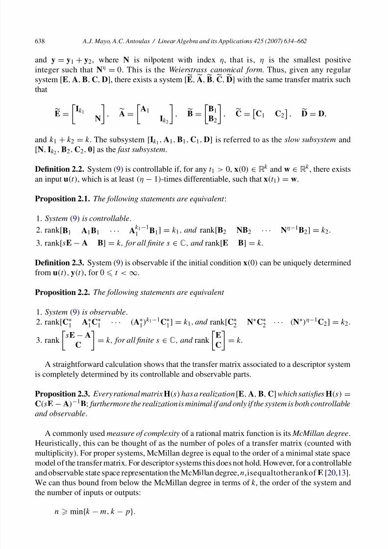
638 A.J. Mayo, A.C. Antoulas / Linear Algebra and its Applications 425 (2007) 634–662
and y = y1 + y2, where N is nilpotent with index η, that is, η is the smallest positiveinteger such that Nη = 0. This is the Weierstrass canonical form. Thus, given any regularsystem [E, A, B, C, D], there exists a system [
E,
A,
B,
C,
D] with the same transfer matrix such
that
E =
Ik1
N
, A =
A1
Ik2
, B =
B1
B2
, C =
C1 C2
, D = D,
and k1 + k2 = k. The subsystem [Ik1 , A1, B1, C1, D] is referred to as the slow subsystem and[N, Ik2 , B2, C2, 0] as the fast subsystem.
Definition 2.2. System (9) is controllable if, for any t 1 > 0, x(0) ∈ Rk and w ∈ R
k, there existsan input u(t), which is at least (η − 1)-times differentiable, such that x(t 1) = w.
Proposition 2.1. The following statements are equivalent :
1. System (9) is controllable.
2. rank[B1 A1B1 · · · Ak1−11 B1] = k1, and rank[B2 NB2 · · · Nη−1B2] = k2.
3. rank[sE − A B] = k, for all finite s ∈ C, and rank[E B] = k.
Definition 2.3. System (9) is observable if the initial condition x(0) can be uniquely determinedfrom u(t), y(t), for 0 t < ∞.
Proposition 2.2. The following statements are equivalent
1. System (9) is observable.
2. rank[C∗1 A∗
1C∗1 · · · (A∗
1)k1−1C∗1] = k1, and rank[C∗
2 N∗C∗2 · · · (N∗)η−1C2] = k2.
3. rank
sE − A
C
= k, for all finite s ∈ C, and rank
E
C
= k.
A straightforward calculation shows that the transfer matrix associated to a descriptor systemis completely determined by its controllable and observable parts.
Proposition 2.3. Every rational matrix H(s) has a realization [E, A, B, C] which satisfies H(s) =
C(sE − A)−1B; furthermore the realization is minimal if and only if the system is both controllable
and observable.
A commonly used measure of complexity of a rational matrix function is its McMillan degree.Heuristically, this can be thought of as the number of poles of a transfer matrix (counted withmultiplicity). For proper systems, McMillan degree is equal to the order of a minimal state spacemodel of the transfer matrix. For descriptor systems this does not hold. However, for a controllableand observable state space representation the McMillan degree, n,isequaltotherankof E [20,13].
We can thus bound from below the McMillan degree in terms of k, the order of the system andthe number of inputs or outputs:
n min{k − m, k − p}.
7/28/2019 Main Loewner Matrix
http://slidepdf.com/reader/full/main-loewner-matrix 6/29
A.J. Mayo, A.C. Antoulas / Linear Algebra and its Applications 425 (2007) 634–662 639
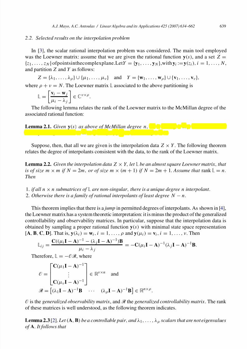
2.2. Selected results on the interpolation problem
In [3], the scalar rational interpolation problem was considered. The main tool employedwas the Loewner matrix: assume that we are given the rational function y(s), and a set Z =
{z1, . . . , zN } ofpointsinthecomplexplane.LetY = {y1, . . . , yN },with yi := y(zi ), i = 1, . . . , N ,and partition Z and Y as follows:
Z = {λ1, . . . , λρ } ∪ {μ1, . . . , μν } and Y = {w1, . . . , wρ } ∪ {v1, . . . , vν },
where ρ + ν = N . The Loewner matrix L associated to the above partitioning is
L =
vi − wj
μi − λj
∈ C
ν×ρ .
The following lemma relates the rank of the Loewner matrix to the McMillan degree of theassociated rational function:
Lemma 2.1. Given y(s) as above of McMillan degree n, let L be any ν × ρ Loewner matrix
corresponding to the set Z × Y. If min{ν, ρ} n, the rank of L is n.
Suppose, then, that all we are given is the interpolation data Z × Y . The following theoremrelates the degree of interpolants consistent with the data, to the rank of the Loewner matrix.
Lemma 2.2. Given the interpolation data Z × Y, let L be an almost square Loewner matrix , that
is of size m × m if N = 2m, or of size m × (m + 1) if N = 2m + 1. Assume that rank L = n.
Then
1. if all n × n submatrices of L are non-singular , there is a unique degree n interpolant .
2. Otherwise there is a family of rational interpolants of least degree N − n.
This theorem implies that there is a jump in permitted degrees of interpolants. As shown in [4],the Loewner matrix has a system theoretic interpretation: it is minus the product of the generalizedcontrollability and observability matrices. In particular, suppose that the interpolation data isobtained by sampling a proper rational function y(s) with minimal state space representation[A, B, C, D]. That is, y(λi ) = wi , i = 1, . . . , ρ and y(μi ) = vi , i = 1, . . . , ν. Then
Lij =C((μi I − A)−1 − (λj I − A)−1)B
μi − λj = −C(μi I − A)−1(λj I − A)−1B.
Therefore, L = −OR, where
O =
⎡⎢⎣
C(μ1I − A)−1
...
C(μν I − A)−1
⎤⎥⎦ ∈ R
ν×n and
R =
(λ1I − A)−1B · · · (λρ I − A)−1B
∈ Rn×ρ .
O is the generalized observability matrix , andR the generalized controllability matrix . The rank
of these matrices is well understood, as the following theorem indicates.
Lemma 2.3 [2]. Let (A, B) be a controllable pair , and λ1, . . . , λρ scalars that are not eigenvalues
of A. It follows that

7/28/2019 Main Loewner Matrix
http://slidepdf.com/reader/full/main-loewner-matrix 7/29
640 A.J. Mayo, A.C. Antoulas / Linear Algebra and its Applications 425 (2007) 634–662
rank[(λ1I − A)−1B · · · (λρ I − A)−1B] = size(A),
provided that ρ n.
This result yields a proof of Lemma 2.1: a Loewner matrix constructed from a function of McMillan degree n, can be factored as a product of a rank n matrix with full column rank and arank n matrix with full row rank, and hence the Loewner matrix must have rank n.
As demonstrated in [2], the above results generalize to matrix interpolation data in a straight-forward manner. For Loewner matrices, the (i,j)th block is
Lij =Vi − Wj
μi − λj
.
The generalized controllability and observability matrices for matrix data, involve block rowsand block columns.
Special case. Suppose that we consider scalar interpolation data consisting of a single pointwith multiplicity, namely: (s0; φ0, φ1, . . . , φN −1), i.e. the value of a function at s0 and that of anumber of its derivatives are provided. It can be shown (see [3]) that the Loewner matrix in thiscase becomes
L =
⎡⎢⎢⎢⎢⎢⎢⎢⎢⎣
φ11!
φ22!
φ33!
φ44!
· · ·
φ22!
φ33!
φ44!
· · ·
φ33!
φ44!
φ44!
.... . .
.
..
⎤⎥⎥⎥⎥⎥⎥⎥⎥⎦
, (10)
and has Hankel structure. Thus the Loewner matrix generalizes the Hankel matrix when interpo-lation at finite points is considered. For connections between Hankel and Loewner matrices seealso [10].
3. The Loewner and the shifted Loewner matrices
The Loewner matrix and the shifted Loewner matrix are both of dimension ν × ρ, and aredefined in terms of the data (3) and (5) as follows
L =
⎡⎢⎢⎣v1r1−1w1
μ1−λ1· · · v1rρ −1wρ
μ1−λρ
.... . .
...vν r1−ν w1
μν −λ1· · ·
vν rρ −ν wρ
μν −λρ
⎤⎥⎥⎦ , σ L =
⎡⎢⎢⎣μ1v1r1−λ11w1
μ1−λ1· · · μ1v1rρ −λρ 1wρ
μ1−λρ
.... . .
...μν vν r1−λ1ν w1
μν −λ1· · ·
μν vν rρ −λρ ν wρ
μν −λρ
⎤⎥⎥⎦ .
(11)
Notice that each entry shown above, for instancevi rj −i wj
μi −λj , is scalar, and is obtained by taking
appropriate inner products of left and right data. If we assume the existence of a rational matrixfunction, H(s), that generates the data then, as the name suggests, the shifted-Loewner matrix
is the Loewner matrix corresponding to sH(s). These matrices satisfy the following Sylvesterequations
L− M L = LW − VR , σ L− Mσ L = LW− M VR (12)

7/28/2019 Main Loewner Matrix
http://slidepdf.com/reader/full/main-loewner-matrix 8/29
A.J. Mayo, A.C. Antoulas / Linear Algebra and its Applications 425 (2007) 634–662 641
The first consequence of these equations is
Proposition 3.1. There holds: σ L − L = VR and σ L − M L = LW.
Proof. Multiplying the equation for L by on the right and subtracting the equation for σ L weobtain
(σ L − L− VR)− M(σ L − L− VR) = 0.
If and M have no eigenvalues in common, the solution to this Sylvester equation is zero, whichyields the desired equality. Correspondingly, if we multiply the equation for L on the left by M
and subtract from it the equation for σ L, by the same reasoning we obtain the second equality.
We can also study the Loewner matrix by assuming the existence of an underlying interpolant,say H(s) = C(sE − A)−1B + D. Following [2], we make use of the fact that the Loewner matrixhas a system theoretically significant factorization, namely it can be factored as a product of the tangential generalized controllability and tangential generalized observability matrices. Fordescriptor systems, this factorization is
L = −YEX, where Y =
⎡⎢⎣
1C(μ1E − A)−1
...
ν C(μν E − A)−1
⎤⎥⎦ ,
X =
(λ1E − A)−1Br1 · · · (λρ E − A)−1Brρ
.
Likewise,σ L = −YAX + LDR.
Y and X are themselves solutions to Sylvester equations:
−AX + EX = BR, (13)
−YA + M YE = LC. (14)
Remark 3.1. In [2] state space models are constructed by factoring the Loewner matrix L todefine Y and X, and then use these equations (with E = I) to construct A, B, C, D.
The following is the descriptor system version of a theorem proved in [2].
Lemma 3.1. Let (E, A, B) be a controllable triple of order k, and λ1, . . . , λρ scalars that are
not generalized eigenvalues of (A, E). Then the rank of the generalized controllability matrix is
k. That is,
rank[(λ1E − A)−1B · · · (λρ E − A)−1B] = k,
provided that ρ k.
This is easily proved by showing that this matrix is of the same rank as the controllabilitymatrix given in [9].
A straight forward corollary to this is a well known result for scalar rational functions, that if the dimension of the Loewner matrix exceeds the degree of the function, then the Loewner matrix
7/28/2019 Main Loewner Matrix
http://slidepdf.com/reader/full/main-loewner-matrix 9/29
642 A.J. Mayo, A.C. Antoulas / Linear Algebra and its Applications 425 (2007) 634–662
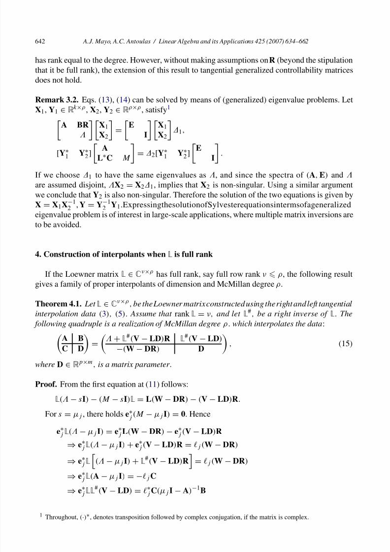
has rank equal to the degree. However, without making assumptions on R (beyond the stipulationthat it be full rank), the extension of this result to tangential generalized controllability matricesdoes not hold.
Remark 3.2. Eqs. (13), (14) can be solved by means of (generalized) eigenvalue problems. LetX1, Y1 ∈ R
k×ρ , X2, Y2 ∈ Rρ×ρ , satisfy1
A BR
X1
X2
=
E
I
X1
X2
1,
[Y∗1 Y∗
2]
A
L∗C M
= 2[Y∗
1 Y∗2]
E
I
.
If we choose 1 to have the same eigenvalues as , and since the spectra of (A, E) and are assumed disjoint, X2 = X21, implies that X2 is non-singular. Using a similar argument
we conclude that Y2 is also non-singular. Therefore the solution of the two equations is given byX = X1X−1
2 , Y = Y−12 Y1.ExpressingthesolutionofSylvesterequationsintermsofageneralized
eigenvalue problem is of interest in large-scale applications, where multiple matrix inversions areto be avoided.
4. Construction of interpolants when L is full rank
If the Loewner matrix L ∈ Cν×ρ has full rank, say full row rank ν ρ, the following result
gives a family of proper interpolants of dimension and McMillan degree ρ.
Theorem 4.1. Let L ∈ Cν×ρ , be the Loewner matrix constructed using the right and left tangential
interpolation data (3), (5). Assume that rank L = ν, and let L#, be a right inverse of L. The
following quadruple is a realization of McMillan degree ρ. which interpolates the data:A B
C D
=
+ L
#(V − LD)R L#(V − LD)
−(W − DR) D
, (15)
where D ∈ Rp×m, is a matrix parameter .
Proof. From the first equation at (11) follows:L(− sI) − (M − sI)L = L(W − DR) − (V − LD)R.
For s = μj , there holds e∗j (M − μj I) = 0. Hence
e∗j L(− μj I) = e∗
j L(W − DR) − e∗j (V − LD)R
⇒ e∗j L(− μj I) + e∗
j (V − LD)R = j (W − DR)
⇒ e∗j L
(− μj I) + L
#(V − LD)R
= j (W − DR)
⇒ e∗j L(A − μj I) = −j C
⇒ e∗j LL
#(V − LD) = ∗j C(μj I − A)−1B
1 Throughout, (·)∗, denotes transposition followed by complex conjugation, if the matrix is complex.

7/28/2019 Main Loewner Matrix
http://slidepdf.com/reader/full/main-loewner-matrix 10/29
A.J. Mayo, A.C. Antoulas / Linear Algebra and its Applications 425 (2007) 634–662 643
⇒ (vj − j D) = j C(μj I − A)−1B
⇒ j [C(μj I − A)−1B + D] = vj
which proves that the left tangential interpolation conditions are satisfied. To prove that the righttangential conditions are also satisfied we notice that the solution xi of the equation
[− λi I + L#(V − LD)R]xi = L
#(V − LD)Rei ,
is xi = ei ; thus
C(λi I − A)−1Bri
= (W − DR)[− λi I + L#(VR − LDR)]−1
L#(V − LD)ri = wi − Dri ,
which implies the desired right tangential interpolation conditions. Notice that interpolation does
not depend on D.
It readily follows that the condition for this realization to be well defined is that none of theinterpolation points be an eigenvalue of A. This can also be achieved by appropriately restrictingD, so that the following equations are satisfied:
det[− sI + L#(V − LD)R] /= 0
for all s = λi and s = μj . We refer to the examples section for an illustration of this issue.Furthermore, since is diagonal, the constructed system is controllable provided that none of therows of L#(V − LD) is zero; this can always be achieved by appropriate choice of D; similarly,
observability can be guaranteed by appropriate choice of D.Finally, it should be noticed that the poles of the constructed systems will vary. The freedom
lies in choosing a generalized inverse of L and D. Thus for a fixed L#, the choice of poles of the
constructed systemis obtained by means of constant output feedback of the system+ L
# VR R
L# L
.
Consequently, in the case m = p = 1, the eigenvalues of the constructed system are obtained bymeans of a rank one perturbation of the right interpolation points :
A = + L#(V − δL)R, δ ∈ R,
where δ = D. It should be noticed that a similar expression for the A matrix of the interpolant
appears in [12].
5. The general tangential interpolation problem
In this section we will present conditions for the solution of the general tangential interpolationproblem by means of state space matrices [E, A, B, C, D]. The first fundamental result is asfollows. Expression (16) for the transfer function below generalizes (8).
Lemma 5.1. Assume that ρ = ν and let det(xL − σ L) /= 0, for all x ∈ {λi } ∪ {μj }. Then E =
−L, A = −σ L , B = V, and C = W is a minimal realization of an interpolant of the data. That
is, the function
H(s) = W(σ L − sL)−1V, (16)
interpolates the data.

7/28/2019 Main Loewner Matrix
http://slidepdf.com/reader/full/main-loewner-matrix 11/29
644 A.J. Mayo, A.C. Antoulas / Linear Algebra and its Applications 425 (2007) 634–662
Proof. Multiplying the first equation of (12) by s and subtracting it from the second we get
(σ L − sL)− M(σ L − sL) = LW(− sI) − (M − sI)VR. (17)
Multiplying this equation by ei on the right and setting s = λi , we obtain
(λi I − M)(σ L − λiL)ei = (λi I − M)Vri
⇒ (σ L − λiL)ei = Vri ⇒ Wei = W(σ L − λiL)−1V H(λi )
ri .
Therefore wi = H(λi )ri . This proves the right tangential interpolation property. To prove the lefttangential interpolation property, we multiply the above equation by e∗
j on the left and set s = μj :
e∗j (σ L − μj L)(μj I −) = e∗
j LW(μj I −)
⇒ e
∗
j (σ L
− μj L
) = j W ⇒ e
∗
j V = j W(σ L
− μj L
)
−1
V H(μj )
Therefore vj = j H(μj ).We show now that the realization is controllable. Suppose that there exists v∗ such that
v∗
σ L − λL V
= 0 for some λ ∈ C.
Then v∗σ L = v∗λL and v∗V = 0. Using Proposition 3.1 it follows that either λ ∈ spec() orv∗L = v∗σ L = 0. Both of these are contradictions, so no such v∗ exists and rank[sL − σ L V] =
k. Similarly, one can prove that rank[L V] = k, and so the realization given is controllable.
Observability is proved in the same manner, so the realization is minimal.
The D term
Eqs. (12) can also be written by adding and subtracting the term LDR, where D ∈ Rp×m, is
at this stage a free matrix parameter:
L− M L = L(W − DR) − (V − LD)R , (18)
(σ L − LDR)− M(σ L − LDR) = L(W − DR)− M(V − LD)R . (19)
Thus, in general all realizations of degree k are parameterized as follows:
H(s) = (W − DR)[(σ L − LDR) − sL]−1(V − LD) + D
For D = 0 we recover (16).
5.1. Analysis of the problem in the general case
Recall that given the data (3) and (5), the Loewner and the shifted Loewener matrices areconstructed by solving the Sylvester equations (12). We assume that rank L = n < ν, ρ, thatis, we assume that the Loewner matrix is not full (row or column) rank. The following result
holds.
Lemma 5.2. Given are the right and left tangential interpolation data (3) and (5), respectively.
Matrices
7/28/2019 Main Loewner Matrix
http://slidepdf.com/reader/full/main-loewner-matrix 12/29
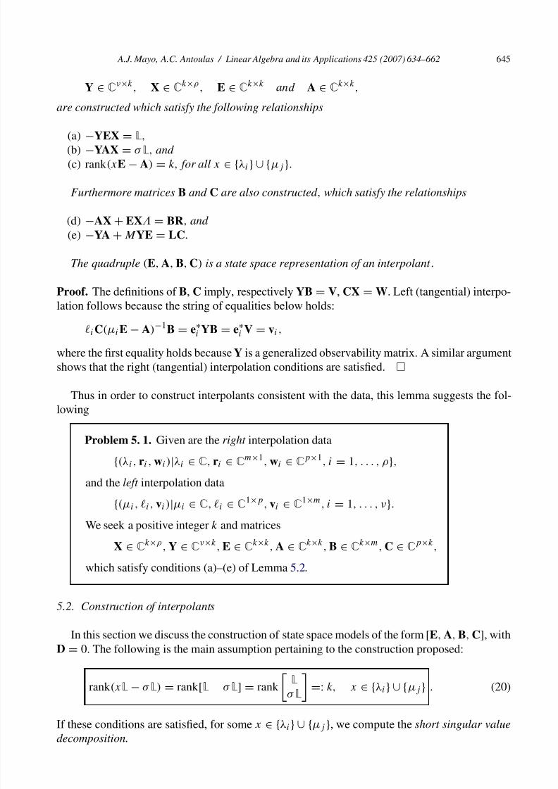
A.J. Mayo, A.C. Antoulas / Linear Algebra and its Applications 425 (2007) 634–662 645
Y ∈ Cν×k , X ∈ C
k×ρ , E ∈ Ck×k and A ∈ C
k×k,
are constructed which satisfy the following relationships
(a) −YEX = L,(b) −YAX = σ L, and
(c) rank(xE − A) = k, for all x ∈ {λi } ∪ {μj }.
Furthermore matrices B and C are also constructed , which satisfy the relationships
(d) −AX + EX = BR, and
(e) −YA + M YE = LC.
The quadruple (E, A, B, C) is a state space representation of an interpolant .
Proof. The definitions of B, C imply, respectively YB = V, CX = W. Left (tangential) interpo-lation follows because the string of equalities below holds:
i C(μi E − A)−1B = e∗i YB = e∗
i V = vi ,
where the first equality holds because Y is a generalized observability matrix. A similar argumentshows that the right (tangential) interpolation conditions are satisfied.
Thus in order to construct interpolants consistent with the data, this lemma suggests the fol-
lowing
Problem 5. 1. Given are the right interpolation data
{(λi , ri , wi )|λi ∈ C, ri ∈ Cm×1, wi ∈ C
p×1, i = 1, . . . , ρ},
and the left interpolation data
{(μi , i , vi )|μi ∈ C, i ∈ C1×p, vi ∈ C
1×m, i = 1, . . . , ν}.
We seek a positive integer k and matrices
X ∈ Ck×ρ , Y ∈ C
ν×k, E ∈ Ck×k , A ∈ C
k×k , B ∈ Ck×m, C ∈ C
p×k,
which satisfy conditions (a)–(e) of Lemma 5.2.
5.2. Construction of interpolants
In this section we discuss the construction of state space models of the form [E, A, B, C], withD = 0. The following is the main assumption pertaining to the construction proposed:
rank(xL
− σ L
) = rank[L
σ L
] = rank L
σ L =: k, x ∈ {λi } ∪ {μj } . (20)
If these conditions are satisfied, for some x ∈ {λi } ∪ {μj }, we compute the short singular value
decomposition.

7/28/2019 Main Loewner Matrix
http://slidepdf.com/reader/full/main-loewner-matrix 13/29
646 A.J. Mayo, A.C. Antoulas / Linear Algebra and its Applications 425 (2007) 634–662
xL − σ L = YX, (21)
where rank(xL − σ L) = rank() = size() =: k, Y ∈ Cν×k and X ∈ C
k×ρ .
Theorem 5.1. With the quantities above, a minimal realization [E, A, B, C], of an interpolant isgiven as follows:
E := − Y∗LX∗
A := − Y∗σ LX∗
B := Y∗V
C := WX∗
⎫⎪⎪⎬⎪⎪⎭ (22)
The proof of this theorem is a special case of the proof of Theorem 5.2 and is thus omitted.Assumption (20) that is imposed demands that the model constructed have full rank tangential
generalized controllability and observability matrices. As noted in the previous section, thiscondition need not hold, so there are cases in which the algorithm does not yield an interpolantwhenonedoesexist.However,forscalarrationalfunctions,thisconditionmusthold(seeCorollary5.1).
Notice that if the directions are not restricted to a subspace, as the amount of data increasesassumption (20) will always be satisfied. Thus generically assumption (20) is always satisfied.Before moving on, we note the following easily verifiable condition for the uniqueness of theassociated rational matrix.
Lemma 5.3. If k − n = min{m, p}, the transfer matrix associated to the constructed model is
the unique interpolant of McMillan degree n.
Proof. The rank k of the singular value decomposition guarantees that no interpolant of orderless than k exists. As the tangential generalized observability and controllability matrices haverank equal to the order of the system, every model of the same order and McMillan degree mustbe equivalent to the constructed model, hence must have the same transfer matrix. Any model of higher order violates (at least) one of the conditions
rank[E B] = k, rank
E
C
= k,
and hence is not minimal.
5.3. Rank properties of L and σ L
To prove that the above procedure produces an interpolant, we need the following fact.
Proposition 5.1. Let V ∈ CN ×n. If the vector v belongs to the column span of the matrix V, for
any matrix W ∈ CN ×n such that W∗V = In, VW∗v = v.
The first result which helps explain why assumption (20) has been imposed is
Lemma 5.4. Let [E, A, B, C] be a minimal state space representation of order k. Given also
are L, R, , M, such that the associated tangential generalized observability matrix Y has full

7/28/2019 Main Loewner Matrix
http://slidepdf.com/reader/full/main-loewner-matrix 14/29
A.J. Mayo, A.C. Antoulas / Linear Algebra and its Applications 425 (2007) 634–662 647
column rank k, and the corresponding tangential generalized controllability matrix X has full
row rank k; none of the interpolation points are poles, and ρ, ν k. Then (20) holds.
Proof. Clearly, rank(xL − σ L) = k. Notice that
[L σ L] = −Y
EX AX
= −Y[E A]
X
X
,
where Y has by assumption full column rank; we claim that [EX AX] has full row rank, forif we assume that there exists a row vector of appropriate dimension z which lies in the leftkernel of this matrix, then zEX = 0 and zAX = 0, which implies that z(xE − A)X = 0, for allx ∈ {λi } ∪ {μj }; but since (xE − A) is invertible and X has full row rank, z must be zero, whichproves that
EX AX
has full row rank k. Consequently the product of a full column rank
matrix, and a full row rank matrix, has the required property rank([L σ L]) = k. The second
equality can be proven similarly.
This lemma implies that in the scalar case condition (20) is necessary and sufficient for theexistence of interpolants.
Corollary 5.1. Given the scalar data L, R, V, W, an interpolant E, A, B, C of order k ρ, ν,
exists if , and only if , assumption (20) holds.
Proof. The sufficiency of (20) follows from Theorem 5.1. Its necessity follows from Lemmas 5.4and 3.1.
Lemma 5.5. Let L, σ L, be the Loewner and the shifted Loewner matrices satisfying (20) for
some set of ρ + ν points. The left and right kernels of xL − σ L are the same for each value of x.
Proof. We will prove this only for the right kernel. First, it is clear that kerL
σ L
⊆ ker(xL − σ L).
As the dimensions of the kernels are the same, equality must hold. This is true for each value of x, and so, ker(xL − σ L) does not vary for the different values of x.
Corollary 5.2. Let L, σ L be two matrices satisfying (20) for some set of ρ + ν points. Then
colspan(L), colspan(σ L) ⊆ colspan(xL − σ L).
Corollary 5.3. Recall the short SVD of xL − σ L, given by (21). Then YY∗σ LX∗X = σ L,
YY∗LX∗X = L, YY∗V = V, and WX∗X = W.
This follows directly from the Proposition 5.1 and the fact, implied by Proposition 3.1, thatcolspan V ⊂ colspan Y, and rowspan W ⊂ rowspan X.
5.4. Taking advantage of theD term
Recall that Eqs. (19) are satisfied for all D. In this case the shifted Loewner matrix is replacedby σ L − LDR while V, W are replaced by V − LD, W − DR. Assumption (20) becomes in thiscase

7/28/2019 Main Loewner Matrix
http://slidepdf.com/reader/full/main-loewner-matrix 15/29
648 A.J. Mayo, A.C. Antoulas / Linear Algebra and its Applications 425 (2007) 634–662
rank(xL − σ L + LDR) = rank[L σ L − LDR]
= rank
L
σ L − LDR
=: k, x ∈ {λi } ∪ {μj },
(23)
wherethisrelationshipissatisfiedforsome D ∈ Cp×m. We now restate theconstructionprocedure.
Theorem 5.2. For any x ∈ {λi } ∪ {μj }, take the short singular value decomposition of
xL − σ L + LDR = YX,
where rank(xL − σ L + LDR) = rank = size =: k, and Y ∈ Cν×k and X ∈ C
k×ρ . Define
E := − Y∗LX∗,
A := − Y∗(σ L − LDR)X∗,
B := Y∗(V − LD),
C := (W − DR)X∗.
⎫⎪⎪⎬⎪⎪⎭
(24)
Then [E, A, B, C, D], is a desired realization.
Proof. First, note that
−AX + EX= Y∗(σ L − LDR)X∗X − Y∗LX∗X
= Y∗(σ L − LDR − L)
= Y∗(V − LD)R = BR
where the second equality follows from Proposition 5.1, by noting that (σ L − LDR)XX∗
=σ L − LDR and LXX∗ = L.
Likewise, −YA + M YE = LC.Thus X and Y are, respectively, the generalized controllabilityand observability matrices for the system [E, A, B, C, D].
To prove that the left interpolation conditions are met we do the following calculation:
i C(μi E − A)−1B + i D = e∗i YB + i D
= e∗i YY∗(V − LD) + i D
= e∗i (V − LD) + i D = vi ,
where the first equality holds because Y is the generalized observability matrix, and the secondone holds because colspan(V − LD) ∈ colspan(xL − σ L). The same reasoning holds for the rightinterpolation conditions.
The proof of minimality follows that given for the analogous statement in Lemma 5.1.
6. Tangential interpolation with derivative constraints
We will now show that the approach to interpolation given in this paper can also be applied tothe problem of interpolation with derivative constraints. For the sake of brevity we will outline
the necessary changes. Thus, we will prove up to the analogue of Lemma 5.1, after which thingsproceed as in the simple interpolation case. We distinguish between the cases in which the left andright interpolation points have trivial intersection, and when they do not. The former case will bereferred to as two-sided tangential interpolation, and the latter case as bi-tangential interpolation.
7/28/2019 Main Loewner Matrix
http://slidepdf.com/reader/full/main-loewner-matrix 16/29
A.J. Mayo, A.C. Antoulas / Linear Algebra and its Applications 425 (2007) 634–662 649
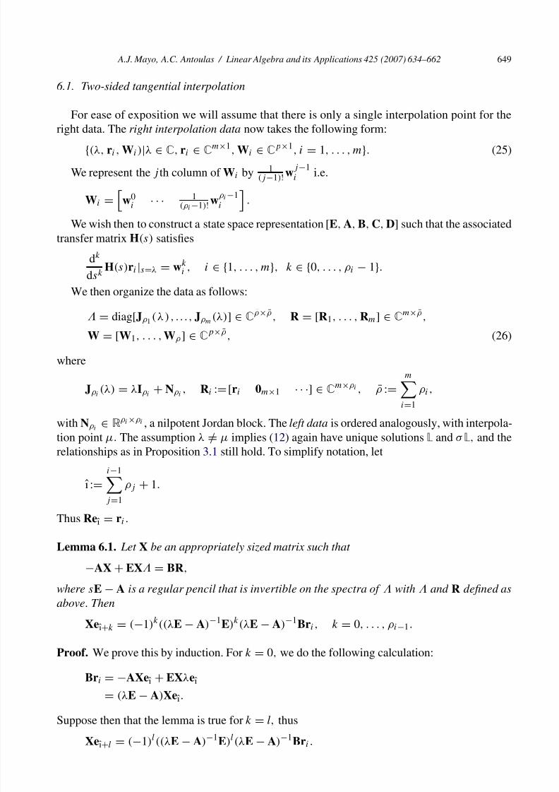
6.1. Two-sided tangential interpolation
For ease of exposition we will assume that there is only a single interpolation point for theright data. The right interpolation data now takes the following form:
{(λ, ri , Wi )|λ ∈ C, ri ∈ Cm×1, Wi ∈ C
p×1, i = 1, . . . , m}. (25)
We represent the j th column of Wi by 1(j −1)! w
j −1i i.e.
Wi =
w0i · · · 1
(ρi −1)!w
ρi −1i
.
We wish then to construct a state space representation [E, A, B, C, D] such that the associatedtransfer matrix H(s) satisfies
dk
dsk
H(s)ri |s=λ = wki , i ∈ {1, . . . , m}, k ∈ {0, . . . , ρi − 1}.
We then organize the data as follows:
= diag[Jρ1 ( λ ) , .. ., Jρm (λ)] ∈ Cρ× ρ , R = [R1, . . . , Rm] ∈ C
m× ρ ,
W = [W1, . . . , Wρ ] ∈ Cp× ρ , (26)
where
Jρi(λ) = λIρi
+ Nρi, Ri := [ri 0m×1 · · ·] ∈ C
m×ρi , ρ :=
mi=1
ρi ,
with Nρi∈ Rρi ×ρi , a nilpotent Jordan block. The left data is ordered analogously, with interpola-
tion point μ. The assumption λ /= μ implies (12) again have unique solutions L and σ L, and therelationships as in Proposition 3.1 still hold. To simplify notation, let
ı :=
i−1j =1
ρj + 1.
Thus Reı = ri .
Lemma 6.1. Let X be an appropriately sized matrix such that
−AX + EX = BR,
where sE − A is a regular pencil that is invertible on the spectra of with and R defined as
above. Then
Xeı+k = (−1)k((λE − A)−1E)k (λE − A)−1Bri , k = 0, . . . , ρi−1.
Proof. We prove this by induction. For k = 0, we do the following calculation:
Bri = −AXeı + EXλeı
= (λE − A)Xeı.
Suppose then that the lemma is true for k = l, thus
Xeı+l = (−1)l ((λE − A)−1E)l(λE − A)−1Bri .
7/28/2019 Main Loewner Matrix
http://slidepdf.com/reader/full/main-loewner-matrix 17/29
650 A.J. Mayo, A.C. Antoulas / Linear Algebra and its Applications 425 (2007) 634–662
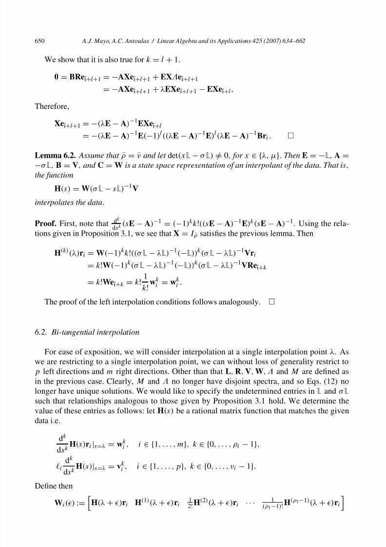
We show that it is also true for k = l + 1.
0 = BReı+l+1 = −AXeı+l+1 + EXeı+l+1
= −AXeı+l+1 + λEXeı+l+1 − EXeı+l,
Therefore,
Xeı+l+1 = −(λE − A)−1EXeı+l
= −(λE − A)−1E(−1)l ((λE − A)−1E)l (λE − A)−1Bri .
Lemma 6.2. Assume that ρ = ν and let det(xL − σ L) /= 0, for x ∈ {λ, μ}. Then E = −L, A =
−σ L, B = V, and C = W is a state space representation of an interpolant of the data. That is,
the function
H(s) = W(σ L
− sL
)
−1
Vinterpolates the data.
Proof. First, note that dk
dsk (sE − A)−1 = (−1)kk!((sE − A)−1E)k (sE − A)−1. Using the rela-tions given in Proposition 3.1, we see that X = I ρ satisfies the previous lemma. Then
H(k)(λ)ri = W(−1)kk!((σ L − λL)−1(−L))k (σ L − λL)−1Vri
= k!W(−1)k(σ L − λL)−1(−L))k(σ L − λL)−1VReı+k
= k!Weı+k = k!1
k!wk
i
= wk
i
.
The proof of the left interpolation conditions follows analogously.
6.2. Bi-tangential interpolation
For ease of exposition, we will consider interpolation at a single interpolation point λ. Aswe are restricting to a single interpolation point, we can without loss of generality restrict top left directions and m right directions. Other than that L, R, V, W, and M are defined as
in the previous case. Clearly, M and no longer have disjoint spectra, and so Eqs. (12) nolonger have unique solutions. We would like to specify the undetermined entries in L and σ L
such that relationships analogous to those given by Proposition 3.1 hold. We determine thevalue of these entries as follows: let H(s) be a rational matrix function that matches the givendata i.e.
dk
dskH(s)ri |s=λ = wk
i , i ∈ {1, . . . , m}, k ∈ {0, . . . , ρi − 1},
idk
dskH(s)|s=λ = vk
i , i ∈ {1, . . . , p}, k ∈ {0, . . . , νi − 1}.
Define then
Wi () :=
H(λ + )ri H(1)(λ + )ri12!
H(2)(λ + )ri · · · 1(ρ1−1)!
H(ρ1−1)(λ + )ri

7/28/2019 Main Loewner Matrix
http://slidepdf.com/reader/full/main-loewner-matrix 18/29
A.J. Mayo, A.C. Antoulas / Linear Algebra and its Applications 425 (2007) 634–662 651
and
:=+ I.
For any /= 0, if we replace W by W and by , Eqs. (12) now have unique solutions that
we denote by L and σ L . We are then interested in these in the limit as tends to zero. As before,let
ı :=
i−1j =1
ρj + 1 and ˆ j =
j −1i=1
νi + 1.
Lemma 6.3. Let L := lim→0 L , and σ L := lim→0 σ L . Then
L(ı+u)(ˆ j+v) =1
(u + v + 1)!i H(u+v+1)(λ)rj , and
σ L(ı+u)( j+v) =1
(u + v + 1)! λi H(u+v+1)(λ)rj + (u + v + 1)i H(u+v)(λ)rj ,
for u = 0, . . . , νi − 1, v = 0, . . . , ρj − 1, i = 1, . . . , p, j = 1, . . . , m .
Theselemmasareeasilyprovedusing Taylor series. They indicate that theadditional constraintsrequired are bi-tangential constraints on higher order derivatives of the desired function. Forexample, in the W data matrix, we are given only up to the ρi th derivative in the directionri ; likewise, in the V data matrix, we are given only up to the νj th derivative in the directionj . However, we see that we require a term involving a derivative of order ρi + νj − 1. There-fore, we will assume that we are also given data that stipulates the values for the following
quantities:
uH(q) (λ)rv for u = 1, . . . , p, v = 1, . . . , m, q = max{ρv, νu}, . . . , ρv + νu − 1.
(27)
Remark 6.1. Suppose that we sample a rational matrix function H(s) and appropriate derivativesthereof at λ ∈ C along left directions 1, . . . , p and right directions r1, . . . , rm Let Lk be a matrixwhose rows are those directions i such that νi k. Let also ν := max{ν1, . . . , νp}. Define Rk
and ρ analogously. Then we can find permutation matrices P and Q such that
P LQ =
⎡⎢⎢⎢⎢⎣L1H(1)R1
12!L1H(2)R2 · · ·
1ρ!L1H(ρ)Rρ
12!L2H(2)R1
13!L2H(3)R2 · · · 1
(ρ+1)!L2H(ρ+1)Rρ
......
. . ....
1ν!Lν H(ν)R1
1(ν+1)!
Lν H(ν+1)R2 · · · 1(ν+ρ−1)!
Lν H(ν+ρ−1)Rρ
⎤⎥⎥⎥⎥⎦ , (28)
and
P σ LQ = λP LQ+
⎡
⎢⎢⎢⎢⎢⎣
L1H(0)R1 L1H(1)R2 · · · 1(ρ−1)!
L1H(ρ−1)Rρ
L2H(1)
R1
12!
L2H(2)
R2 · · · 1
(ρ)!L2H(ρ)
Rρ
... ... . . . ...
1(ν−1)!
Lν H(ν−1)R11
(ν)!Lν H(ν)R2 · · · 1
(ν+ρ−2)!Lν H(ν+ρ−2)Rρ
⎤
⎥⎥⎥⎥⎥⎦ .
(29)

7/28/2019 Main Loewner Matrix
http://slidepdf.com/reader/full/main-loewner-matrix 19/29
652 A.J. Mayo, A.C. Antoulas / Linear Algebra and its Applications 425 (2007) 634–662
Notice that if ν = ν1 = · · · = νp and ρ = ρ1 = · · · = ρm, then these matrices have block Hankel
structure. Furthermore, if the directions are the canonical basis, then these expressions are thoseof the Loewner and shifted Loewner matrices for MIMO interpolation with derivative constraint.
Proposition 6.1. L and σ L satisfy σ L − L = VR and σ L − M L = LW, where
= diag[Jρ1 ( t ) , . . . , Jρρ(t)], M = diag[J∗
ν1( t ) , . . . , J∗
νν(t)],
and W, V, L and σ L are as above.
Proof. We prove that σ L − L = VR. Note that if we multiply the left hand side by eˆ j+v thedefinitions of L and σ L imply that we get 0 unless v = 0. Clearly, Re j+v = 0 if v /= 0, so we justhave to check the equality when v = 0.
(σ L − L)eˆ j =
⎡⎢⎢⎢⎢⎢⎢⎢⎢⎢⎢⎣
10!
1H(0)rj
1(1)!
1H(1)rj
...1
(ν1−1)!1H(ν1−1)rj
...1
(v+νp −1)!pH(νp −1)rj
⎤⎥⎥⎥⎥⎥⎥⎥⎥⎥⎥⎦= Vrj = VRe j.
We conclude by proving the analogue of Lemma 5.1.
Lemma 6.4. Assume that ρ = ν and let det(λL − σ L) /= 0. Then
E = −L, A = −σ L, B = V, C = W,
is a minimal realization of an interpolant of the data. That is, the function
H(s) = W(σ L − sL)−1V
interpolates the data.
Proof. By the same reasoning as in the previous section, H(s) satisfies the two-sided tangentialinterpolation conditions i.e. H(k)(λ)r
i= wk
i, k ρ
i, i = 1, . . . , m , and
iH(k)(λ) = vk
i, k ν
i,
i = 1, . . . , p. As before, dk
dsk (sE − A)−1 = (−1)k k!((sE − A)−1E)k(sE − A)−1. Choose a, b
such that a + b = k and a ρv − 1, b νu − 1. Then
dk
dsk(sE − A)−1 = (−1)kk!(sE − A)−1[E(sE − A)−1]a−1E[(sE − A)−1E]b(sE − A)−1.
Then
i H(k)(λ)rj = i [(−1)k k!(σ L − λL)−1((−L)(σ L − λL)−1)a−1
×(−L)((σ L − λL)−1(−L))b(σ L − λL)−1]rj .
On the right, using Proposition 6.1 we see that X = Iρ satisfies Lemma 6.1. Thus
(−1)q ((σ L − λL)−1(−L))q (σ L − λL)−1VReı+q = eı+q .
7/28/2019 Main Loewner Matrix
http://slidepdf.com/reader/full/main-loewner-matrix 20/29
A.J. Mayo, A.C. Antoulas / Linear Algebra and its Applications 425 (2007) 634–662 653
Likewise, on the left, we have
e∗ı+p−1(σ L − λL)−1((−L)(σ L − λL))−1)p−1(−1)p−1 = e∗
ı+p−1.
Thus
i H(k)(λ)rj = k!(−1)e∗ı+p−1(−L)e j+q = k!
1
(p + q)!H
(p+q)ij (λ) = H
(p+q)ij (λ).
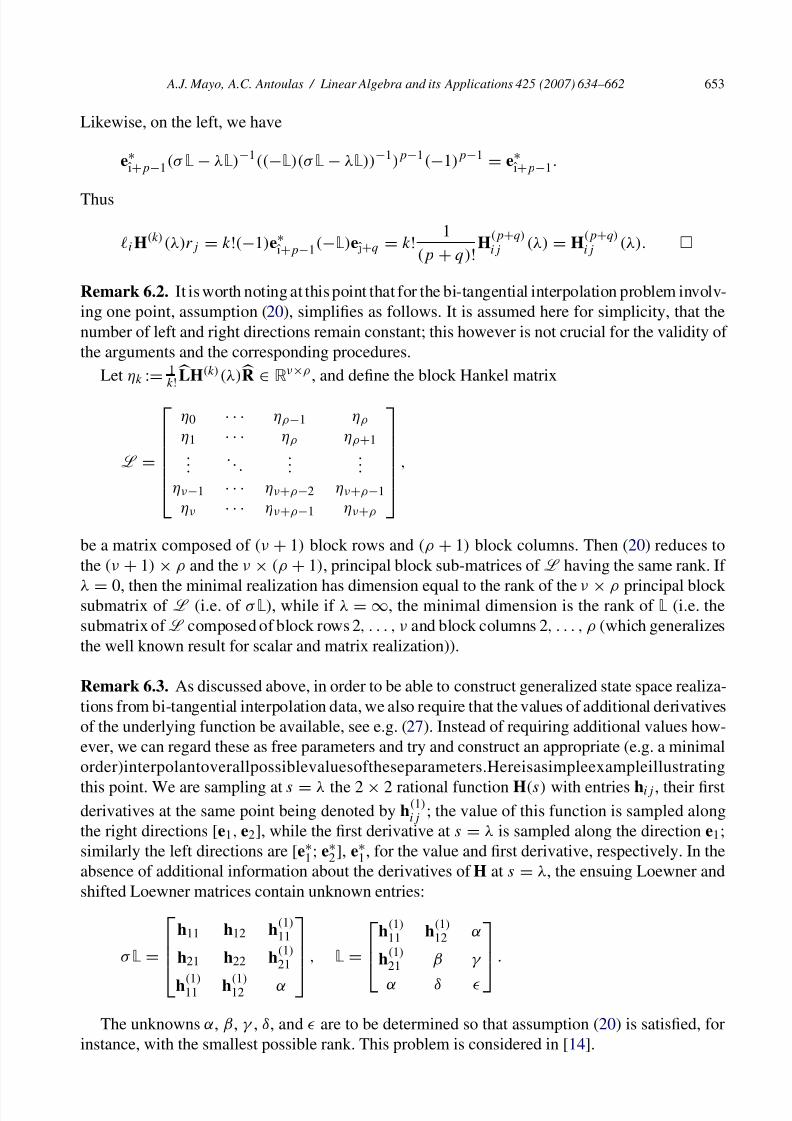
Remark 6.2. It is worth noting at this point that for the bi-tangential interpolation problem involv-ing one point, assumption (20), simplifies as follows. It is assumed here for simplicity, that thenumber of left and right directions remain constant; this however is not crucial for the validity of the arguments and the corresponding procedures.
Let ηk := 1k!LH(k)(λ)R ∈ R
ν×ρ , and define the block Hankel matrix
L =
⎡⎢⎢⎢⎢⎢⎣
η0 · · · ηρ−1 ηρ
η1 · · · ηρ ηρ+1...
. . ....
...
ην−1 · · · ην+ρ−2 ην+ρ−1
ην · · · ην+ρ−1 ην+ρ
⎤⎥⎥⎥⎥⎥⎦ ,
be a matrix composed of (ν + 1) block rows and (ρ + 1) block columns. Then (20) reduces tothe (ν + 1) × ρ and the ν × (ρ + 1), principal block sub-matrices of L having the same rank. If
λ = 0, then the minimal realization has dimension equal to the rank of the ν × ρ principal blocksubmatrix of L (i.e. of σ L), while if λ = ∞, the minimal dimension is the rank of L (i.e. thesubmatrix of L composed of block rows 2, . . . , ν and block columns 2, . . . , ρ (which generalizesthe well known result for scalar and matrix realization)).
Remark 6.3. As discussed above, in order to be able to construct generalized state space realiza-tions from bi-tangential interpolation data, we also require that the values of additional derivativesof the underlying function be available, see e.g. (27). Instead of requiring additional values how-ever, we can regard these as free parameters and try and construct an appropriate (e.g. a minimalorder)interpolantoverallpossiblevaluesoftheseparameters.Hereisasimpleexampleillustrating
this point. We are sampling at s = λ the 2 × 2 rational function H(s) with entries hij , their firstderivatives at the same point being denoted by h
(1)ij ; the value of this function is sampled along
the right directions [e1, e2], while the first derivative at s = λ is sampled along the direction e1;similarly the left directions are [e∗
1; e∗2], e∗
1, for the value and first derivative, respectively. In theabsence of additional information about the derivatives of H at s = λ, the ensuing Loewner andshifted Loewner matrices contain unknown entries:
σ L =
⎡
⎢⎢⎣h11 h12 h
(1)11
h21 h22 h(1)21
h(1)11 h(1)12 α
⎤
⎥⎥⎦, L =
⎡
⎢⎣h
(1)11 h
(1)12 α
h(1)21 β γ
α δ
⎤
⎥⎦.
The unknowns α, β, γ , δ, and are to be determined so that assumption (20) is satisfied, forinstance, with the smallest possible rank. This problem is considered in [14].

7/28/2019 Main Loewner Matrix
http://slidepdf.com/reader/full/main-loewner-matrix 21/29
654 A.J. Mayo, A.C. Antoulas / Linear Algebra and its Applications 425 (2007) 634–662
7. Parametrization of interpolants
For the scalar case, we will show that the parameter D denoted by δ here, parameterizes allinterpolants of the given degree. Note that in the scalar case, L is taken to be the column vector
of appropriate length with ones in all of its entries. Likewise, R is the row vector with ones inall of its entries. When specifying an interpolation condition, we will therefore not include thedirection. Recall that in the scalar case there is a family of interpolants if, and only if, the Loewnermatrix is square (ρ = ν) and non-singular. Therefore this assumption will hold for this section.Noting that in this case sL − σ L + δLR is a rank one perturbation of sL − σ L, the followingholds.
Lemma 7.1. With = (σ L − sL)−1, there holds:
(W−
δR)[−1 −
δLR]−1
(V−
δL)+
δ=
δ
(1 − WL)(1 − RV)
(1 − δRL)+
W
V. (30)
It is hereby assumed that the pencil sL − σ L is regular .
For the proof we will make use of the Sherman–Morrison–Woodbury formula:
(A + BDC)−1 = A−1 − A−1B(D−1 + CA−1B)−1CA−1,
which in the case that B = b is a single column, C = c a single row, and consequently D = δ, isa scalar, becomes
(A + δbc)−1 = A−1 − A−1
bcA−1
δ−1 + cA−1b= A−1 − δ A
−1bcA
−1
1 + δcA−1b.
Proof. We have
(W − δR)(−1 + (−δ)LR)−1(V − δL) + δ
= (W − δR)(V − δL) a
+ δ(W − δR)LR(V − δL)
(1 − δRL) b
+ δ,
a = WV − δRV − δWL + δ2RL,
(1 − δRL) · b = δWLRV − δ2RLRV − δ2WLRL + δ3RLRL, (31)
(1 − δRL) · a = (1 − δRL) · (WV − δRV − δWL + δ2RL)
= WV − δRV − δWL + δ2RL
− δRL · (WV − δRV − δWL + δ2RL)
= WV − δRV − δWL + δ2RL
− δRLWV + δ2RLRV + δ2RLWL − δ3RLRL, (32)
δ(1 − δRL) = δ − δ2RL. (33)
7/28/2019 Main Loewner Matrix
http://slidepdf.com/reader/full/main-loewner-matrix 22/29
A.J. Mayo, A.C. Antoulas / Linear Algebra and its Applications 425 (2007) 634–662 655
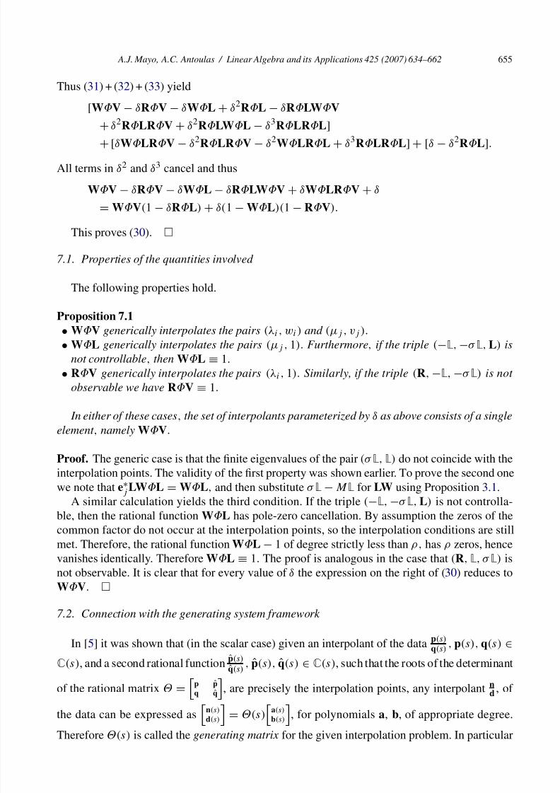
Thus (31) + (32) + (33) yield
[WV − δRV − δWL + δ2RL − δRLWV
+ δ2RLRV + δ2RLWL − δ3RLRL]
+ [δWLRV − δ2RLRV − δ2WLRL + δ3RLRL] + [δ − δ2RL].
All terms in δ2 and δ3 cancel and thus
WV − δRV − δWL − δRLWV + δWLRV + δ
= WV(1 − δRL) + δ(1 − WL)(1 − RV).
This proves (30).
7.1. Properties of the quantities involved
The following properties hold.
Proposition 7.1
• WV generically interpolates the pairs (λi , wi ) and (μj , vj ).
• WL generically interpolates the pairs (μj , 1). Furthermore, if the triple (−L, −σ L, L) is
not controllable, then WL ≡ 1.
• RV generically interpolates the pairs (λi , 1). Similarly, if the triple (R, −L, −σ L) is not
observable we have RV ≡ 1.
In either of these cases, the set of interpolants parameterized by δ as above consists of a singleelement , namely WV.
Proof. The generic case is that the finite eigenvalues of the pair (σ L,L) do not coincide with theinterpolation points. The validity of the first property was shown earlier. To prove the second onewe note that e∗
j LWL = WL, and then substitute σ L − M L for LW using Proposition 3.1.A similar calculation yields the third condition. If the triple (−L, −σ L, L) is not controlla-
ble, then the rational function WL has pole-zero cancellation. By assumption the zeros of thecommon factor do not occur at the interpolation points, so the interpolation conditions are stillmet. Therefore, the rational function WL − 1 of degree strictly less than ρ, has ρ zeros, hence
vanishes identically. Therefore WL ≡ 1. The proof is analogous in the case that (R, L, σ L) isnot observable. It is clear that for every value of δ the expression on the right of (30) reduces toWV.
7.2. Connection with the generating system framework
In [5] it was shown that (in the scalar case) given an interpolant of the data p(s)q(s)
, p(s), q(s) ∈
C(s), and a second rational function p(s)
q(s), p(s), q(s) ∈ C(s), such that the roots of the determinant
of the rational matrix = p p
q q, are precisely the interpolation points, any interpolant n
d, of
the data can be expressed as
n(s)
d(s)
= (s)
a(s)
b(s)
, for polynomials a, b, of appropriate degree.
Therefore (s) is called the generating matrix for the given interpolation problem. In particular

7/28/2019 Main Loewner Matrix
http://slidepdf.com/reader/full/main-loewner-matrix 23/29
656 A.J. Mayo, A.C. Antoulas / Linear Algebra and its Applications 425 (2007) 634–662
if happens to be column reduced with same column indices, say k, then all interpolants of McMillan degree k, are obtained by choosing a and b constant.
We will now show that the expression in Lemma 7.1 yields indeed a generating matrix. Eq.(30) can be written as a linear fraction:
WV + δ[(1 − WL)(1 − RV) − (WV)(RL)]
1 − δRL(34)
There are two generating systems involved in the above relationship:
1(s) =
WV (1 − WL)(1 − RV)
1 0
,
2(s) =
WV (WV)(RL) − (1 − WL)(1 − RV)
1 RL
,
which are both rational. Notice that the determinant of these generating systems has zeros at theinterpolating points λi and μj . Clearly
2(s) = 1(s)
1 RL
0 −1
.
This implies that the quotient of the entries of the second column of 2 yields an interpolantas well, namely
(WV)(RL) − (1 − WL)(1 − RV)
RL.
It follows that this interpolant has the same degree as WV.
Finally a parametrization of all interpolants p/q of the given degree is given byp
q
= 2(s)
1δ
=
WV + δ[(WV)(RL) − (1 − WL)(1 − RV)]
1 + δRL
.
The above results are illustrated next.
8. Examples
The results of the preceding sections will now be illustrated by means of a few simple examples.
8.1. Example A
A =
⎡⎣1 0 0
0 1 00 0 0
⎤⎦ , E =
⎡⎣0 −1 0
0 0 00 0 1
⎤⎦ , B =
⎡⎣0 1
1 00 1
⎤⎦ , C =
1 0 00 1 1
.
Thus the transfer function is
H(s) = C(sE − A)−1B =
s −1
−1 1s
.
We will now recover this system by sampling its transfer function directionally. The choseninterpolation data are: = diag([1, 2, 3]), M = diag([−1, −2, −3, −4]), while
L =
⎡⎢⎢⎣1 −11 −21 −31 0
⎤⎥⎥⎦ , R =
1 1 01 2 1
.
7/28/2019 Main Loewner Matrix
http://slidepdf.com/reader/full/main-loewner-matrix 24/29
A.J. Mayo, A.C. Antoulas / Linear Algebra and its Applications 425 (2007) 634–662 657
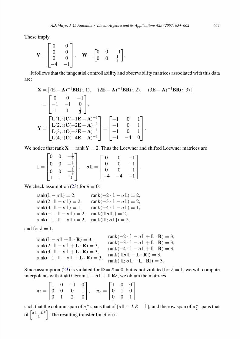
These imply
V =
⎡
⎢⎢⎣0 00 0
0 0−4 −1
⎤
⎥⎥⎦ , W = 0 0 −1
0 013 .
It follows that the tangential controllability and observability matrices associated with this dataare:
X =
(E − A)−1BR(:, 1), (2E − A)−1BR(:, 2), (3E − A)−1BR(:, 3)]
=
⎡⎣ 0 0 −1
−1 −1 01 1 1
3
⎤⎦ ,
Y =
⎡⎢⎢⎣L(1, :)C(−1E − A)−1L(2, :)C(−2E − A)−1
L(3, :)C(−3E − A)−1
L(4, :)C(−4E − A)−1
⎤⎥⎥⎦ =
⎡⎢⎢⎣−1 0 1−1 0 1−1 0 1−1 −4 0
⎤⎥⎥⎦ .
We notice that rank X = rank Y = 2. Thus the Loewner and shifted Loewner matrices are
L =
⎡⎢⎢⎢⎣
0 0 − 13
0 0 − 13
0 0 − 13
1 1 0
⎤⎥⎥⎥⎦
, σ L =
⎡⎢⎢⎣
0 0 −10 0 −10 0 −1
−4
−4
−1
⎤⎥⎥⎦
.
We check assumption (23) for δ = 0:
rank(L − σ L) = 2,
rank(2 · L − σ L) = 2,
rank(3 · L − σ L) = 1,
rank(−1 · L − σ L) = 2,
rank(−1 · L − σ L) = 2,
rank(−2 · L − σ L) = 2,
rank(−3 · L − σ L) = 2,
rank(−4 · L − σ L) = 1,
rank([Lσ L]) = 2,
rank([L; σ L]) = 2,
and for δ = 1:
rank(L − σ L + L · R) = 3,
rank(2 · L − σ L + L · R) = 3,
rank(3 · L − σ L + L · R) = 3,
rank(−1 · L − σ L + L · R) = 3,
rank(−2 · L − σ L + L · R) = 3,rank(−3 · L − σ L + L · R) = 3,
rank(−4 · L − σ L + L · R) = 3,
rank([Lσ L − L · R]) = 3,
rank([L; σ L − L · R]) = 3.
Since assumption (23) is violated for D = δ = 0, but is not violated for δ = 1, we will computeinterpolants with δ /= 0. From L − σ L + LRδ, we obtain the matrices
πl =
⎡⎣
1 0 −1 00 0 0 1
0 1 2 0
⎤⎦
, πr =
⎡⎣
1 0 00 1 0
0 0 1
⎤⎦
such that the column span of π ∗l spans that of [σ L − LR L], and the row span of π ∗
2 spans that
of
σ L − LR
L
. The resulting transfer function is
7/28/2019 Main Loewner Matrix
http://slidepdf.com/reader/full/main-loewner-matrix 25/29
658 A.J. Mayo, A.C. Antoulas / Linear Algebra and its Applications 425 (2007) 634–662
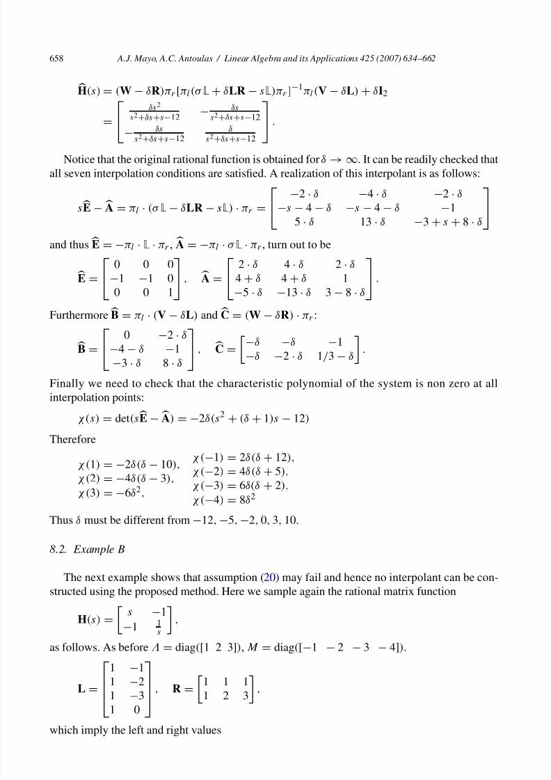
H(s) = (W − δR)πr [πl (σ L + δLR − sL)πr ]−1πl (V − δL) + δI2
=
⎡⎣
δs2
s2+δs+s−12− δs
s2+δs+s−12
−
δs
s2+δs+s−12
δ
s2+δs+s−12
⎤⎦
.
Notice that the original rational function is obtained for δ → ∞. It can be readily checked thatall seven interpolation conditions are satisfied. A realization of this interpolant is as follows:
sE −A = πl · (σ L − δLR − sL) · πr =
⎡⎣ −2 · δ −4 · δ −2 · δ
−s − 4 − δ −s − 4 − δ −15 · δ 13 · δ −3 + s + 8 · δ
⎤⎦
and thus E = −πl · L · πr , A = −πl · σ L · πr , turn out to be
E = ⎡⎣ 0 0 0−1 −1 00 0 1
⎤⎦ , A = ⎡⎣ 2 · δ 4 · δ 2 · δ
4 + δ 4 + δ 1−5 · δ −13 · δ 3 − 8 · δ
⎤⎦ .
FurthermoreB = πl · (V − δL) and C = (W − δR) · πr :
B =
⎡⎣ 0 −2 · δ
−4 − δ −1−3 · δ 8 · δ
⎤⎦ , C =
−δ −δ −1−δ −2 · δ 1/3 − δ
.
Finally we need to check that the characteristic polynomial of the system is non zero at allinterpolation points:
χ(s) = det(sE −A) = −2δ(s2 + (δ + 1)s − 12)
Therefore
χ (1) = −2δ(δ − 10),
χ (2) = −4δ(δ − 3),
χ (3) = −6δ2,
χ (−1) = 2δ(δ + 12),
χ (−2) = 4δ(δ + 5),
χ (−3) = 6δ(δ + 2),
χ (−4) = 8δ2
Thus δ must be different from −12, −5, −2, 0, 3, 10.
8.2. Example B
The next example shows that assumption (20) may fail and hence no interpolant can be con-structed using the proposed method. Here we sample again the rational matrix function
H(s) =
s −1
−1 1s
,
as follows. As before = diag([1 2 3]), M = diag([−1 − 2 − 3 − 4]).
L = ⎡⎢⎢⎣1 −1
1 −21 −31 0
⎤⎥⎥⎦ , R = 1 1 11 2 3 ,
which imply the left and right values

7/28/2019 Main Loewner Matrix
http://slidepdf.com/reader/full/main-loewner-matrix 26/29
A.J. Mayo, A.C. Antoulas / Linear Algebra and its Applications 425 (2007) 634–662 659
V =
⎡⎢⎢⎣
0 00 00 0
−4 −1
⎤⎥⎥⎦
, W =
0 0 00 0 0
.
The resulting tangential controllability and observability matrices are
X =
⎡⎣ 0 0 0
−1 −1 −11 1 1
⎤⎦ , Y =
⎡⎢⎢⎣
−1 0 1−1 0 1−1 0 1−1 −4 0
⎤⎥⎥⎦ ,
and therefore rank X = 1 while rank Y = 2. Finally
L =
⎡⎢⎢⎣
0 0 00 0 0
0 0 01 1 1
⎤⎥⎥⎦ , σ L =
⎡⎢⎢⎣
0 0 00 0 0
0 0 0−4 −4 −4
⎤⎥⎥⎦
Checking assumption (20) we get
rank([Lσ L]) = 1,
rank([L; σ L]) = 1,
rank([L − σ L]) = 1,
rank([2L − σ L]) = 1,
rank([3L − σ L]) = 1,
rank([−L − σ L]) = 1,
rank([−2L − σ L]) = 1,
rank([−3L − σ L]) = 1,
rank([−4L − σ L]) = 0.
while rank([Lσ L − LR]) = 3andrank([L; σ L − LR]) = 2;thelastequalityholdsforany D /= 0.Thus no interpolant can be constructed using the proposed method. In particular the interpolant
provided by this method, namely H(s) =
0 00 0
, satisfies all interpolation conditions, but one.
8.3. Example C
This example incorporates derivative constraints. We are given the following data:
r1 =
11
, r2 =
21
, w0
1 =
00
, w1
1 =
1
−1
w0
2 =
3
− 32
, w1
2 =
2
− 14
on the right and
∗1 =
10
, ∗
2 =
01
, [v0
1]∗ =
−1−1
,
[v11]∗ =
−10
, [v0
2]∗ =
−1− 1
2
, [v1
2]∗ =
0
− 14
on the left. We want to find a rational matrix function H(s) such that Hj −1(i)ri = wj −1i , i , j ∈
{1, 2} and i Hj −1(−i) = vj −1i , i , j ∈ {1, 2}. The data is then arranged as follows:
=
⎡⎢⎢⎣1 1 0 00 1 0 00 0 2 10 0 0 2
⎤⎥⎥⎦ , R =
1 0 2 01 0 1 0
, W =
w0
1 w11 w0
2 w12
,
7/28/2019 Main Loewner Matrix
http://slidepdf.com/reader/full/main-loewner-matrix 27/29
660 A.J. Mayo, A.C. Antoulas / Linear Algebra and its Applications 425 (2007) 634–662
M =
⎡⎢⎢⎣
−1 0 0 01 −1 0 00 0 −2 0
0 0 1 −2
⎤⎥⎥⎦
, L =
⎡⎢⎢⎣
1 00 00 1
0 0
⎤⎥⎥⎦
, V =
⎡⎢⎢⎢⎣
v01
v11
v02
v12
⎤⎥⎥⎥⎦
.
The Loewner and shifted Loewner matrices L, σ L turn out to be
L =
⎡⎢⎢⎣
1 0 2 00 0 0 012 − 1
214 − 1
814 − 1
418 − 1
16
⎤⎥⎥⎦ , σ L =
⎡⎢⎢⎣
−1 1 1 21 0 2 0
−1 0 −2 00 0 0 0
⎤⎥⎥⎦ .
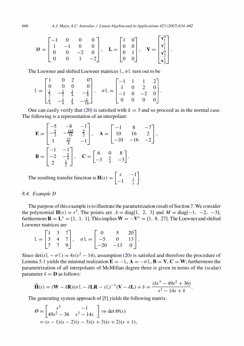
One can easily verify that (20) is satisfied with k = 3 and so proceed as in the normal case.The following is a representation of an interpolant:
E =
⎡⎢⎣−5 −8 −1− 5
2 − 18516
52
1 378 −1
⎤⎥⎦ , A =
⎡⎣ −1 8 −7
10 16 2−10 −16 −2
⎤⎦ ,
B =
⎡⎣−1 −1
−2 − 54
2 12
⎤⎦ , C =
6 0 8
−3 54 −3
.
The resulting transfer function is H(s) = s −1
−11s .
8.4. Example D
The purpose of this example is to illustrate the parametrization result of Section 7. We considerthe polynomial H(s) = s3. The points are = diag[1, 2, 3] and M = diag[−1, −2, −3];furthermore R = L∗ = [1, 1, 1]. This implies W = −V∗ = [1, 8, 27]. The Loewner and shiftedLoewner matrices are
L =
⎡⎣
1 3 73 4 77 7 9
⎤⎦ , σ L =
⎡⎣
0 5 20−5 0 13
−20 −13 0
⎤⎦ .
Since det(sL − σ L) = 4s(s2 − 14), assumption (20) is satisfied and therefore the procedure of Lemma 5.1 yields the minimal realization E = −L, A = −σ L, B = V, C = W; furthermore theparametrization of all interpolants of McMillan degree three is given in terms of the (scalar)parameter δ = D as follows:
H(s) = (W − δR)(σ L − δLR − sL)−1(V − δL) + δ =(δs 3 − 49s2 + 36)
s3 − 14s + δ.
The generating system approach of [5] yields the following matrix:
= s3 −1
49s2 − 36 s3 − 14s
⇒ det(s)
= (s − 1)(s − 2)(s − 3)(s + 3)(s + 2)(s + 1),

7/28/2019 Main Loewner Matrix
http://slidepdf.com/reader/full/main-loewner-matrix 28/29
A.J. Mayo, A.C. Antoulas / Linear Algebra and its Applications 425 (2007) 634–662 661
which implies that all interpolants are obtained by taking linear combinations of the two rowsand forming the quotient of the first over the second entry. This is exactly the expression obtainedabove. Therefore we obtain a parametrization of all interpolants of McMillan degree three. Thepolynomial s3 that we started out with is obtained for δ → ∞.
8.5. Example E
We are given the rational matrix
H(s) =
s2
s + 1,
1
s + 1
,
which is sampled with r =
11
at λ = 0. Thus the following samples are obtained:
H(0)
(0) = [01],H(1)(0) = [0 − 1],
H(2)(0) = [11],
H(3)(0) = [−1 − 1],
h0 = H(0)
(0)r = 1,h1 = H(1)(0)r = −1,
h2 = H(2)(0)r = 2,
h3 = H(3)(0)r = −2,
h4 = H(4)
(0)r = 2,h5 = H(5)(0)r = −2,
h6 = H(6)(0)r = 2,
h7 = H(7)(0)r = −2,
where H(k)(0) = 1k!
dk Hdsk |s=0, k = 0, 1, . . . , 7. Following (28) and (29), the Loewner and shifted
Loewner matrices are
L =
⎡
⎢⎢⎣h1 h2 h3 h4
h2 h3 h4 h5
h3
h4
h5
h6h4 h5 h6 h7
⎤
⎥⎥⎦=
⎡
⎢⎢⎣−1 2 −2 22 −2 2 −2
−2 2 −2 22 −2 2 −2
⎤
⎥⎥⎦,
σ L =
⎡⎢⎢⎣
h0 h1 h2 h3
h1 h2 h3 h4
h2 h3 h4 h5
h3 h4 h5 h6
⎤⎥⎥⎦ =
⎡⎢⎢⎣
1 −1 2 −2−1 2 −2 22 −2 2 −2
−2 2 −2 2
⎤⎥⎥⎦ .
Then, the quadruple (E, A, B, C), where E = −L3 = −L(1 : 3, 1 : 3), A = −σ L3 = −σ L(1 :
3, 1 : 3),
B = ⎡⎣H(0)(0)
H(1)(0)
H(2)(0)⎤⎦ = ⎡⎣0 1
0 −11 1
⎤⎦ , C = [h0 h1 h2] = [1 − 1 2],
is a minimal realization of the data:
C(sE − A)−1B =
s2
s + 1,
1
s + 1
= H(s).
9. Conclusions
In this paper we present a framework for the construction of matrix rational interpolants H, ingeneralized state space form, given tangential interpolation data. We thus construct generalizedstate space realizations (E, A, B, C, D), where E may be singular, such that
H(s) = C(sE − A)−1B + D,
7/28/2019 Main Loewner Matrix
http://slidepdf.com/reader/full/main-loewner-matrix 29/29
662 A.J. Mayo, A.C. Antoulas / Linear Algebra and its Applications 425 (2007) 634–662
from tangential interpolation data. We call this thegeneralized realization problem. Central objectsfor this construction are the Loewner matrix L, and the shifted Loewner matrix σ L, associatedwith the data; σ L is introduced here for the first time. The approach parallels the solution of the realization problem in which state space representations (A, B, C) are constructed given the
Hankel matrix of Markov parameters, that is given interpolation data at infinity.
References
[1] A.C. Antoulas, Approximation of large-scale dynamical systems, Advances in Design and Control, vol. DC-06,SIAM, Philadelphia, 2005.
[2] B.D.O. Anderson, A.C. Antoulas, Rational interpolation and state variable realizations, Linear Algebra Appl.137/138 (1990) 479–509.
[3] A.C. Antoulas, B.D.O. Anderson, On the scalar rational interpolation problem, IMA J. Math. Control Inform. 3(1986) 61–68.
[4] A.C. Antoulas, B.D.O. Anderson, State space and polynomial approaches to rational interpolation, Progr. Systems
Control Theory, Proceedings MTNS-89 3 (1989) 73–82.[5] A.C. Antoulas, J.A. Ball, J. Kang, J.C. Willems, On the solution of the minimal rational interpolation problem,
Linear Algebra Appl. 137/138 (1990) 511–573.[6] J. Ball, I. Gohberg, L. Rodman, Interpolation of Rational Matrix Functions, Operator Theory: Advances and
Applications, vol. 45, Birkhäuser, 1990.[7] V. Belevitch, Interpolation Matrices, Philips Res. Repts. (1970) 337–369.[8] P. Benner, V.I. Sokolov, Partial realization of descriptor systems, Syst. Control Lett. 55 (11) (2006) 929–938.[9] L. Dai, Singular control systems, Lecture Notes in Control and Information Sciences, Springer-Verlag, Berlin, 1989.
[10] M. Fiedler, Hankel and Loewner matrices, Linear Algebra Appl. 58 (1984) 75–95.[11] K. Gallivan, A. Vandendorpe, P. Van Dooren, Model reduction of MIMO systems via tangential interpolation, SIAM
J. Matrix Anal. Appl. 26 (2004) 328–349.
[12] S. Gugercin, A.C. Antoulas, C. Beattie, First-order necessary conditions and a rational Krylov iteration for optimalH2 model reduction, submitted for publication.[13] M. Kuijper, J.M. Schumacher, Realization of autoregressive equations in pencil and descriptor form,SIAM J. Control
Optimiz. SICON-58 (1990) 1162–1189.[14] A.J. Mayo, Interpolation from a realization point of view, Ph.D. Dissertation, Department of Electrical and Computer
Engineering, Rice University, 2007.[15] A.J. Mayo, A.C. Antoulas, New results on interpolation and model reduction, in: Proc. 17th Intl. Symposium on
Math. Theory of Networks and Systems, MTNS06, Kyoto, 2006, pp. 1643–1651.[16] R. Nevanlinna, Über Beschränkte analytische Funktionen, Ann. Acad. Sci. Fenn. A 32 (7) (1929).[17] G. Pick, Über die Beschränkungen analytischer Funktionen, welche durch vorgegebene Funktionswerte bewirkt
sind, Math. Ann. 77 (1916) 7–23.[18] H.H. Rosenbrock, Structural properties of linear dynamical systems, Int. J. Control 20 (1974) 191–202.
[19] T. Stykel, Gramian based model reduction for descriptor systems, Math. Control Signals Syst. MCSS-16 (2004)297–319.
[20] G.C. Verghese, B.C. Levy, T. Kailath, A generalized state-space for singular systems, IEEE Trans. Aut. Contr. AC-26(1981) 811–831.
[21] D.C. Youla, M. Saito, Interpolation with positive real functions, J. Franklin Inst. 284 (1967) 77–108.[22] Ph. Delsarte, Y. Genin, Y. Kamp, On the role of the Nevanlinna–Pick problem in circuits and system theory, Circuit
Theory Appl. 9 (1981) 177–187.


![[-2em]Conformally Invariant Processes and the Schramm–Loewner](https://img.pdfslide.us/doc/110x75/5870bfda1a28ab87318b5a40/-2emconformally-invariant-processes-and-the-schrammloewner-.jpg)