Maillage de connexion via unetransformation en ondelettes etinterpolation locale par des RBF

Mesh connection with Wavelet transform and RBF localinterpolation.

PHAN Anh-Cang

Laboratoire des Sciences de l’Information et des Systèmes (LSIS, UMR CNRS 7296)Ecole doctorale mathématiques et informatique de Marseille (ED 184)Campus de Luminy, case postale 925, 13288 Marseille cedex 9, France.

Anh-cang.PHAN@univ-amu.fr

RÉSUMÉ. Nous présentons une méthode de connexion de maillages entre deux domaines maillésde différents niveaux de résolution. Le maillage de liaison est créé à l’aide d’une interpola-tion avec des fonctions de base radiale locale combinée à une transformation en ondelettesB-spline. Cela garantit que la continuité entre les deux zones est préservée et que le maillagede connexion est modifié progressivement pour tenir compte des résolutions différentes entreles deux zones. Cette méthode pourrait être étendue à des applications liées au remplissage detrous, à la couture de maillages de subdivision et à la composition d’objets 3D.

ABSTRACT. We introduce a connection method between two mesh areas at different resolutions.The connecting mesh is based on a local interpolation with radial basis functions and a Lifted B-spline wavelet transform. This ensures that the continuity between these mesh areas is preservedand the connecting mesh is modified gradually in resolution between coarse and fine areas. Thismethod could be expanded to applications related to filling holes, pasting subdivision meshesand composition of 3D objects.

MOTS-CLÉS : transformée en ondelettes; maillage triangulaire; maillage de connexion; ondelettesB-splines.

KEYWORDS: Wavelet transform; triangular meshes; mesh connection; B-spline wavelets.

2 9 èmes Journées des doctorants du LSIS

1. Introduction

Complex shapes are generated by a set of assembled patches or separate meshareas which could be at different resolution levels. Their surfaces could appear cracks,gaps or holes. It leads to a problem about missing surfaces in Computer Aided Design(CAD) applications such as unwanted object shapes, cracks along the boundaries ofthe patches, or even incorrect connections between meshes. To overcome these pro-blems, cracks must be removed. Our work aims at constructing a high quality connec-ting mesh between two selected mesh areas of a model using the Radial Basis Func-tion (RBF) local interpolation and the wavelet transform so that we can preserve thecontinuity between these selected mesh areas to produce a smooth surface.

2. Related work

In many cases, subdivision of the whole input mesh is not necessary, only someareas that need to be subdivided to make them smoother. This is important to re-duce the unnecessary subdivision process, and save the refinement time, the storagespace. Some research (Noor Asma Husain et al., 2011), (Pakdel et al., 2004), (Pak-del et al., 2005), (Husain et al., 2010) related to the incremental subdivision methodwith Butterfly, Loop and Catmull-Clark schemes. The main work of these methodsis to generate a smooth surface by refining only some selected areas of a mesh withthe same a subdivision scheme, and then removing cracks with simple triangulation.However, this simple triangulation has some undesired side-effects. It changes theconnectivity, valence of odd vertices, and the surrounding areas. This not only altersthe limit subdivision surface, but also reduces its smoothness. Moreover, it produceshigh valence vertices which lead to long faces. They create ripple effects on the subdi-vision surface. In addition, there have been also research works relevant to connectingand pasting meshes in (Zhang et al., 2010), (Fu et al., 2004), (Barequet et al., 1995).These methods consist in connecting the meshes of a surface at the same resolutionlevel which adopt various criteria to compute the planar shape from a 3D surface patchby minimizing their differences. The approaches are computationally expensive andmemory consuming. Therefore, we proposed a new mesh connection method withoutneeding to handle cracks, modify original boundaries of mesh areas of a model, andsubdivide the closest faces around the original boundaries.

3. Background

3.1. Wavelet multiresolution representation of curves and surfaces

Wavelet has been applied successfully to a wide variety of applications in mode-ling environment (Mallat, 1998), (Olsen et al., 2008), (Bertram, 2002). Wavelet toolsupports the multiresolution representations of curves and surfaces (Lounsbery et al.,1997), (Eck et al., 1995) ; curve smoothing at different resolution levels (Olsen etal., 2008), (Guskov et al., 1999) ; overall form edition of a curve while preserving itsdetails (Suciati et al., 2009) ; and curve approximation (Stollnitz et al., 1996), (Khoda-kovsky et al., 2000). Recently, multiresolution (MR) settings based on wavelets have

Maillage de connexion via ondelettes et RBF 3

been proposed for many curve and surface subdivision types : B-splines (Bertram etal., 2004), Doo subdivision (Samavati et al., 2002), and Loop (Bertram, 2004). Thewavelet transform allows a decomposition of curves and surfaces at different resolu-tions while maintaining geometric details. Wavelet analysis provides a set of tools torepresent functions hierarchically (Stollnitz et al., 1995). The coarse scaling functionrepresents coarse curves or surfaces, encodes an approximation of the function. Thewavelet function represents the difference between coarse and fine curves or surfaces,and encodes the missing details. These tools can efficiently facilitate geometric mode-ling operations.

The combination of B-splines and wavelets leads to the idea of B-spline wavelets(Bertram et al., 2004). B-spline wavelets form a hierarchical basis for the space ofB-spline curves and surfaces in which every object has a unique representation. Ta-king advantage of the lifting scheme, Lifted B-spline wavelets (Sweldens et al., 1996)are a fast computational tool for multiresolution analysis with a computational com-plexity linear in the number of control points for a given B-spline curve. They allowmultiresolution analysis of B-spline curves, representing a curve at multiple resolutionlevels, editing curves, etc. The Lifted B-spline wavelet transform includes two phases :the forward and the backward B-spline wavelet transforms. From a fine curve at thedecomposition level j+1, Cj+1, the forward B-spline wavelet transform decomposesCj+1 into a sequence of coarser approximations of the curve, Ck (0 ≤ k ≤ j), anddetail (error) vectors. The detail vectors are a set of wavelet cœfficients containingthe geometric differences with respect to the finer levels. The backward B-spline wa-velet transform can be used to reconstruct fine resolution curves from a coarse curveand detail vectors. Given a curve at the decomposition level j, Cj , the backward B-spline wavelet transform synthesis Cj and the detail vectors into the finer curves, Ck

(k ≥ j + 1).

In our approach, we apply the Lifted B-spline wavelet transform for multiresolu-tion analysis of discrete boundary curves. We can expand to apply the other waveletsfor the multiresolution representations of the discrete boundary curves.

3.2. Radial Basis Function (RBF) local interpolation

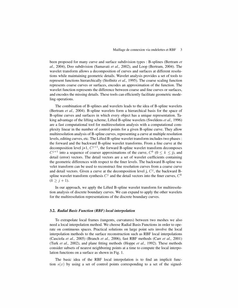
To extrapolate local frames (tangents, curvatures) between two meshes we alsoneed a local interpolation method. We choose Radial Basis Functions in order to ope-rate on continuous spaces. Practical solutions on large point sets involve the localinterpolation methods to the surface reconstruction such as RBF local interpolations(Casciola et al., 2005) (Branch et al., 2006), fast RBF methods (Carr et al., 2001)(Turk et al., 2002), and plane fitting methods (Hoppe et al., 1992). These methodsconsider subsets of nearest neighboring points at a time to compute the local interpo-lation functions on a surface as shown in Fig. 1.

The basic idea of the RBF local interpolation is to find an implicit func-tion s(x) by using a set of control points corresponding to a set of the signed-

4 9 èmes Journées des doctorants du LSIS

Figure 1. Selection of the nearest neighboring points to determine the set of controlpoints for computing the interpolation function.

distance function values. Given a set of N distinct control points (or centers) X ={xk = (xk, yk, zk)}Nk=1 ⊂ R3 corresponding to a set of distance function valuesf = {fk}Nk=1 ⊂ R. For each xk ∈ X, k = 1, ..., N , we determine a subset ofnearest neighboring points Xk = {xk} ∪ {xj ∈ X;xj ∈ Neighbors(xk)} as shownin Fig. 1, where Neighbors(xk) is the nearest neighboring points of xk. Let Ik be theset of indexes of Xk and Nk = |Xk| be the number of the nearest neighbors of xk.

We want to approximate the signed-distance function f(x) by an interpolations(x). An RBF local interpolation function s : R3 → R on Xk is determined by :

sk(x) =∑j∈Ik

λjφ(‖x− xj‖) [1]

It requires satisfying the local interpolation constraints on Xk.

sk(xi) = fi =∑j∈Ik

λjφ(‖xi − xj‖), i ∈ Ik [2]

where φ(‖x− xj‖) are the radial basis functions (RBFs) ; the points xj are refer-red to as the control points of the RBF and are also the nearest neighboring points ofxk ; λj are the weights of the RBFs ; ‖x‖ is the Euclidean norm. The basis functionis normally chosen from the families of the spline functions of smoothing, such as thebiharmonic φ(r) = r (r = ‖x− xj‖), the triharmonic φ(r) = r3, the Gaussian φ(r) =e−(

rh )2 , and so on. In our approach, we choose the Gaussian basis function and h to

be the average distance from xk to the control points xj . Combining eq. 1 and eq. 2leads to :

Maillage de connexion via ondelettes et RBF 5

φ1,1 · · · φ1,Nk

.... . .

...φNk,1 · · · φNk,Nk

λ1

...λNk

=

f1...

fNk

[3]

Equation 3 may be re-written in the matrix form :

ΦXkΛXk

= FXk[4]

where φi,j = φ(||xi − xj ||), ΦXk= (φi,j) with i, j ∈ Ik, ΛXk

=(λ1, λ2, ..., λNk)T , FXk

= (f1, ..., fNk)T . After solving the linear system of eq. 4to compute the unknown weights Λ of the basis functions, a data set is simply recons-tructed by computing the local interpolation function values sk(x) at x ∈ Xk usingeq. 1.

4. Mesh Connection method overview

4.1. Basic concepts and topology representation

Let M l1 and Mk

2 be two meshes and pi, qi their vertices. An edge connecting pito qi is denoted ei or piqi. An edge is usually shared by two faces. If it is shared byonly one, it corresponds to a boundary edge and its end vertices are called boundaryvertices. We need to construct a connecting mesh CM between two meshes M l

1 andMk

2 so that it can preserve the continuity between them as illustrated in Fig. 2.

Figure 2. Basic concepts and topology representation related to the algorithm.

Let us introduce the notations used in the following :

– s : the number of intermediate discrete curves (also called the number of newcreated boundary curves) of CM created between M l

1 and Mk2 (see Fig. 4). It is a user

defined threshold and controls the resolution of CM.– j : the order number of the decomposition step to create intermediate discrete

curves, also called decomposition level. Since two boundary curves between M l1 and

Mk2 will be created in each decomposition level j, 1 ≤ j ≤ s

2 .

6 9 èmes Journées des doctorants du LSIS

– Cj1 and Cj

2 : the two boundary curves of CM at level j which approximate thetwo original boundary curves C0

1 and C02 of meshes M l

1 and Mk2 .

– N(Cj1) : the number of vertices of boundary curve Cj

1 at level j. It correspondsto the density of vertices of the boundary curve Cj

1 .

– pji , qji : the vertices i on boundary curves Cj1 and Cj

2 . (p0i = pi and q0i = qi)

– Lj1 : the list of the boundary vertex pairs (pj−1i , qj−1k ). That means, the boundary

vertices pj−1i ∈ Cj−11 are paired with the boundary vertices qj−1k ∈ Cj−1

2 .

– Lj2 : the list of the boundary vertex pairs (qj−1k , pj−1i ). That means, the boundary

vertices qj−1k ∈ Cj−12 are paired with the boundary vertices pj−1i ∈ Cj−1

1 .

4.2. Algorithm overview

The idea of our algorithm is to create the new boundary curves Cj1 and Cj

2 bet-ween M l

1 and Mk2 based on the previously created boundary curves Cj−1

1 and Cj−12

using the Lifted B-spline wavelet transform and the RBF local interpolation. Then,we connect each new boundary curve Cj

1 to Cj−11 , and Cj

2 to Cj−12 . Cj

1 is created in adirection from Cj−1

1 to Cj−12 and conversely for Cj

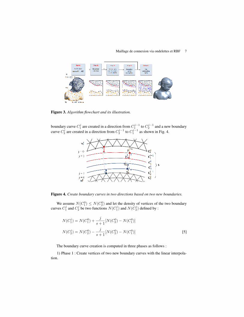
2 . The algorithm (Fig. 3) consistsof the following main steps detailed in the next section :

– Step 1. Boundary detection : read the input geometry model of two subdividedmeshes M l

1 and Mk2 at different resolution levels. Detect and mark boundary vertices

of two boundaries C01 and C0

2 in M l1 and Mk

2 respectively.– Step 2. Boundary vertex pairs and boundary curve creation : pair the boundary

vertices of two boundary curves Cj−11 , Cj−1

2 based on the distance between them. Ifthe distance between them is very narrow, we go to Step 3 to connect the boundarycurve pair (Cj−1

1 ,Cj−12 ). In contrast, we perform a boundary curve creation to create

new boundary curves Cj1 , Cj

2 . It first produces vertices of two new boundary curvesfrom the paired boundary vertices by the linear interpolation method and then projectthem onto the surface CM using the RBF local interpolation method. It finally refineor coarsen these new boundary curves applying the wavelet transforms and vertexinsertion and deletion operations.

– Step 3. Boundary curve connection : perform a boundary triangulation for eachboundary curve pair (Cj−1

1 ,Cj1) and (Cj−1

2 ,Cj2).

– Step 4. Repeat steps 2 through 3 until two mesh areas M l1 and Mk

2 has beenconnected or patched by all newly created triangles.

5. Boundary curve creation and connection

The idea is to create two new boundary curves Cj1 and Cj

2 from the paired verticesin each level j. Paired vertices are obtained by shortest distances between vertices ofeach boundary. That is, new boundary vertices pji ∈ C

j1 and qjk ∈ C

j2 are created by

boundary vertex pairs (pj−1i , qj−1k ) ∈ Lj1 and (qj−1k , pj−1i ) ∈ Lj

2 respectively. A new

Maillage de connexion via ondelettes et RBF 7

Figure 3. Algorithm flowchart and its illustration.

boundary curve Cj1 are created in a direction from Cj−1

1 to Cj−12 and a new boundary

curve Cj2 are created in a direction from Cj−1

2 to Cj−11 as shown in Fig. 4.

Figure 4. Create boundary curves in two directions based on two new boundaries.

We assume N(C01 ) ≤ N(C0

2 ) and let the density of vertices of the two boundarycurves Cj

1 and Cj2 be two functions N(Cj

1) and N(Cj2) defined by :

N(Cj1) = N(C0

1 ) +j

s+ 1[N(C0

2 )−N(C01 )]

N(Cj2) = N(C0

2 )− j

s+ 1[N(C0

2 )−N(C01 )] [5]

The boundary curve creation is computed in three phases as follows :

1) Phase 1 : Create vertices of two new boundary curves with the linear interpola-tion.

8 9 èmes Journées des doctorants du LSIS

- Create vertices of the discrete boundary curve Cj1 in a direction from Cj−1

1

to Cj−12 (see Fig. 4) : for each boundary vertex pair (pj−1i , qj−1k ) ∈ Lj

1, we apply thelinear interpolation equation eq. 6 to create new boundary vertices pji ∈ C

j1 .

pji = pj−1i +j

s+ 1(qj−1k − pj−1i ) [6]

Where i is the index of boundary vertices of Cj1 , 1 ≤ i ≤ N(Cj−1

1 ) and k the indexof boundary vertices of Cj−1

2 , 1 ≤ k ≤ N(Cj−12 ).

- In the same way, we create the new boundary vertices qjk ∈ Cj2 by eq. 7.

qjk = qj−1k +j

s+ 1(pj−1i − qj−1k ) [7]

Where k is the index of a boundary vertex on Cj2 , 1 ≤ k ≤ N(Cj−1

2 ) and i the indexof the boundary vertex on Cj−1

1 , 1 ≤ i ≤ N(Cj−11 ).

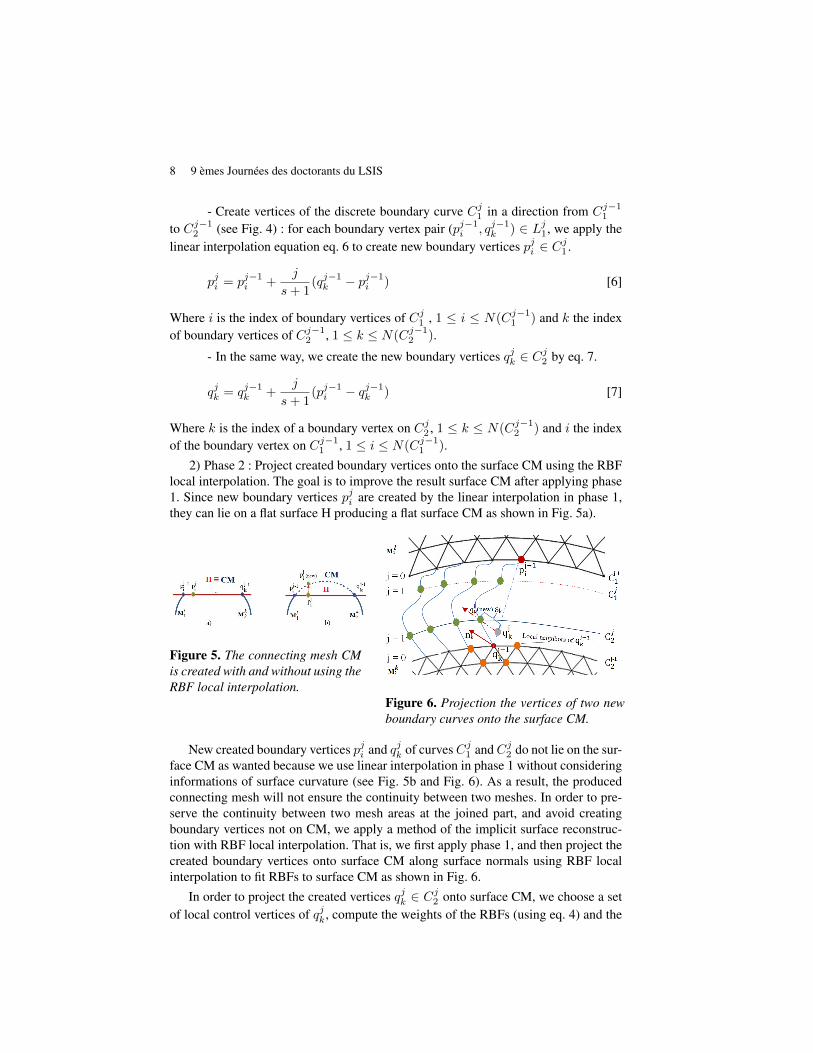
2) Phase 2 : Project created boundary vertices onto the surface CM using the RBFlocal interpolation. The goal is to improve the result surface CM after applying phase1. Since new boundary vertices pji are created by the linear interpolation in phase 1,they can lie on a flat surface H producing a flat surface CM as shown in Fig. 5a).

Figure 5. The connecting mesh CMis created with and without using theRBF local interpolation.

Figure 6. Projection the vertices of two newboundary curves onto the surface CM.

New created boundary vertices pji and qjk of curvesCj1 andCj

2 do not lie on the sur-face CM as wanted because we use linear interpolation in phase 1 without consideringinformations of surface curvature (see Fig. 5b and Fig. 6). As a result, the producedconnecting mesh will not ensure the continuity between two meshes. In order to pre-serve the continuity between two mesh areas at the joined part, and avoid creatingboundary vertices not on CM, we apply a method of the implicit surface reconstruc-tion with RBF local interpolation. That is, we first apply phase 1, and then project thecreated boundary vertices onto surface CM along surface normals using RBF localinterpolation to fit RBFs to surface CM as shown in Fig. 6.

In order to project the created vertices qjk ∈ Cj2 onto surface CM, we choose a set

of local control vertices of qjk, compute the weights of the RBFs (using eq. 4) and the

Maillage de connexion via ondelettes et RBF 9

local interpolation function values sk for these vertices (using eq. 1). Then, we projectthem onto surface CM with the projection distances sk along normals of vertices qj−1k

and update the vertices of boundary curve Cj2 as their projected vertices. Similarly, we

also apply the same for the created vertices pji ∈ Cj1 .

In general, it is not necessary to use such a large number of off-surface vertices.Theoretically, a single off-surface vertex might be sufficient for the surface reconstruc-tion. Therefore, we propose to introduce a set of local control vertices Qk correspon-ding to each vertex qjk for the local reconstruction of the RBF interpolation functionas follows :

- Qk = Q1 ∪Q2,- Q1 = {qj−1k } ∪ {q1 ∈ Neighbors(qj−1k )}. Q1 is the local neighbors of qj−1k

referred to as on-surface vertices,- Q2 = {q2 = q1 + d ∗ n(q1); q1 ∈ Q1}, d is the projection distance defined by

user, n(q1) is the normal of the vertex q1. Q2 is referred to as off-surface vertices.A set of local control vertices Qk corresponding to a set of distance function values :f(q) = 0 for q ∈ Q1 and f(q) = d for q ∈ Q2.

3) Phase 3 : Refine or coarsen these new boundary curves with the wavelet trans-forms. Since the number of vertices of Cj

1 and Cj2 is now N(Cj−1

1 ) and N(Cj−12 )

respectively, we need to increase and reduce the resolutions of Cj1 and Cj

2 must beN(Cj

1) and N(Cj2). We apply the Lifted B-spline wavelet transform for the multire-

solution representations of the boundary curveCj1 andCj

2 to refine the boundary curveCj

1 , coarsen the boundary curve Cj2 . Then, we perform the vertex insertion or deletion

operations to control the density of vertices of Cj1 and Cj

2 . The result is to obtain twoboundary curves Cj

1 with the density of vertices N(Cj1) and Cj

2 with the density ofvertices N(Cj

2). This ensures that the connecting mesh CM is changed gradually inresolution from one area of the surface to another area.

After creating two boundary curves Cj1 and Cj

2 , we connect each new boundarycurve to each previously created boundary curve : Cj−1

1 to Cj1 and Cj−1

2 to Cj2 based

on the method of stitching the matching borders proposed by (Barequet et al., 1995).The basic idea is the implementation of the boundary triangulation based on the dis-tance between boundary vertices. We consider the distance between three adjacentvertices of two boundaries before connecting them together to create a triangular face(see Fig. 5). This process terminates when we reach the last vertices of both bounda-ries.

Figure 7. Figure shows boundary curve connection.

10 9 èmes Journées des doctorants du LSIS

6. Results

Our algorithm has been implemented on Matlab. All experimental results in thispaper were obtained on a PC 2.27GHz CPU Core i5 with 3GB Ram. We have appliedour algorithm to various types of 3D objects. From two original coarse mesh areasM0

1

and M02 of a model, we apply Loop scheme at level 2 for M0

1 and Butterfly schemeat level 1 for M0

2 to obtain two subdivided mesh areas M21 and M1

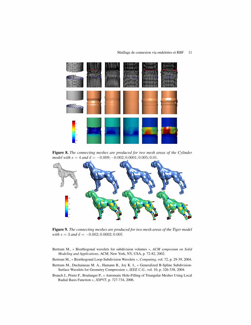
2 . We then applyour CM2D-RBFW algorithm for connecting them. Results are shown as in Fig. 8 andFig. 9 which illustrate the change of different values of s and d. They show images ofresulting meshes (the top row), surfaces (the middle row), and the Gaussian curvatures(the bottom row).

The number of intermediate discrete curves s and the distance function value dare parameters defined by user. In our approach, the initial constraint for d in [− t

2 ,t2 ],

where t is chosen to be the average distance between pi ∈ C01 , qk ∈ C0

2 and their localneighbors. That is, to create off-surface vertices, on-surface vertices are projected atmost distance t

2 . This assumption is naturally satisfied in almost all practical appli-cations (Alexa et al., 2003). This figures show the reconstruction of the Cylinder andthe Tiger with and without validation of values d. The resulting surfaces are deformedwhen taking invalid projection distance values d = −0.009;−0.002; 0.005; 0.01 forthe Cylinder and d = −0.002; 0.005 for the Tiger. The surface of the Cylinder and theTiger is visually smooth when choosing a valid projection distance value d = 0.0001and d = 0.0002 respectively.

The experimental results show that our approach satisfies the constraint of thecontinuity between mesh areas and produces high quality and smooth connectingmeshes.

7. Conclusion

We introduced a new incremental simple and efficient method which generates ahigh quality connecting mesh and a smooth surface. The surface is changed graduallyin resolution from one area of the surface to another area. The algorithm additionallydoesn’t subdivide the closest faces around selection areas of a mesh model. The resultsof our method show high quality connecting meshes and smooth surfaces. In addition,smooth surfaces generated by our method have proper connectivity and geometry. Ourmethod could be extended to applications related to filling holes, pasting subdivisionmeshes and incremental subdivisions. We are now working on a scheme to subdividethe connecting mesh when the two meshes are subdivided again so that the connectionremains valid.

8. Bibliographie

Alexa M., Behr J., Cohen-Or D., Fleishman S., Levin D., Silva C. T., « Computing and Rende-ring Point set surfaces », IEEE-Vis.Comp.Graph, vol. 9, p. 3-15, January, 2003.

Barequet G., Sharir M., « Filling gaps in the boundary of a polyhedron », Computer AidedGeometric Design, vol. 12, p. 207-229, 1995.

Maillage de connexion via ondelettes et RBF 11

Figure 8. The connecting meshes are produced for two mesh areas of the Cylindermodel with s = 4 and d = −0.009;−0.002; 0.0001; 0.005; 0.01.

Figure 9. The connecting meshes are produced for two mesh areas of the Tiger modelwith s = 3 and d = −0.002; 0.0002; 0.005

Bertram M., « Biorthogonal wavelets for subdivision volumes », ACM symposium on SolidModeling and Applications, ACM, New York, NY, USA, p. 72-82, 2002.

Bertram M., « Biorthogonal Loop-Subdivision Wavelets », Computing, vol. 72, p. 29-39, 2004.

Bertram M., Duchaineau M. A., Hamann B., Joy K. I., « Generalized B-Spline Subdivision-Surface Wavelets for Geometry Compression », IEEE C.G., vol. 10, p. 326-338, 2004.

Branch J., Prieto F., Boulanger P., « Automatic Hole-Filling of Triangular Meshes Using LocalRadial Basis Function », 3DPVT, p. 727-734, 2006.

12 9 èmes Journées des doctorants du LSIS

Carr J. C., Beatson R. K., Cherrie J. B., Mitchell T. J., Fright W. R., McCallum B. C., EvansT. R., « Reconstruction and representation of 3D objects with radial basis functions », SIG-GRAPH ’01, New York, NY, USA, p. 67-76, 2001.

Casciola G., Lazzaro D., Montefusco L. B., Morigi S., « Fast surface reconstruction and holefilling using Radial Basis Functions, Numerical Algorithms », 2005.

Eck M., DeRose T., Duchamp T., Hoppe H., Lounsbery M., Stuetzle W., « Multiresolutionanalysis of arbitrary meshes », SIGGRAPH ’95, New York, NY, USA, p. 173-182, 1995.

Fu H., Tai C.-L., Zhang H., « Topology-Free Cut-and-Paste Editing over Meshes », GMP,p. 173-184, 2004.

Guskov I., Sweldens W., Schröder P., « Multiresolution Signal Processing for Meshes », in ,A. Rockwood (ed.), SIGGRAPH ’99, p. 325-334, August 8–13, 1999.

Hoppe H., DeRose T., Duchamp T., McDonald J., Stuetzle W., « Surface reconstruction fromunorganized points », SIGGRAPH Comput. Graph., vol. 26, p. 71-78, July, 1992.

Husain N. A., Bade A., Kumoi R., Rahim M. S. M., « Iterative selection criteria to improvesimple adaptive subdivision surfaces method in handling cracks for triangular meshes »,VRCAI ’10, ACM, New York, NY, USA, p. 207-210, 2010.

Khodakovsky A., Schröder P., Sweldens W., « Progressive Geometry Compression », SIG-GRAPH ’01, New York, p. 271-278, July 23–28, 2000.

Lounsbery M., DeRose T., Warren J. D., « Multiresolution Analysis for Surfaces of ArbitraryTopological Type. », ACM Trans. Graph.p. 34-73, 1997.

Mallat S. G., A Wavelet Tour of Signal Processing, Academic Press, 1998.

Noor Asma Husain M. S. M. R., Bade A., « Iterative Process to Improve Simple AdaptiveSubdivision Surfaces Method with Butterfly Scheme », WAS, Tech, p. 622-626, 2011.

Olsen L. J., Samavati F. F., « A Discrete Approach to Multiresolution Curves and Surfaces »,IEEE Computer Society, Washington, DC, USA, p. 468-477, 2008.

Pakdel H.-R., Samavati F. F., « Incremental Adaptive Loop Subdivision », vol. 3045 of LectureNotes in Computer Science, Springer, p. 237-246, May 14-17, 2004.

Pakdel H.-R., Samavati F. F., « Incremental Catmull-Clark Subdivision », IEEE Computer Sco-ciety, p. 95-102, Jun 13-16, 2005.

Samavati F. F., Mahdavi-Amiri N., Bartels R. M., « Multiresolution Surfaces having ArbitraryTopologies by a Reverse Doo Subdivision Method », C.G. Forum, vol. 21, p. 121-136, 2002.

Stollnitz E. J., DeRose T. D., Salesin D. H., « Wavelets for Computer Graphics : A Primer, Part1 », IEEE Comput. Graph. Appl., vol. 15, p. 76-84, May, 1995.

Stollnitz E. J., DeRose T. D., Salesin D. H., Wavelets for Computer Graphics : Theory andApplications, Morgan Kaufmann Publishers, Inc., 1996.

Suciati N., Harada K., « Wavelets-based Multiresolution Surface as Framework for Editing theGlobal and Local Shapes », Journal of C.S and N.S, vol. number 5, p. 77-83, 2009.

Sweldens W., Schröder P., « Building Your Own Wavelets at Home », IN WAVELETS IN COM-PUTER GRAPHICS, p. 15-87, 1996.

Turk G., O’brien J. F., « Modelling with implicit surfaces that interpolate », ACM Trans. Graph.,vol. 21, p. 855-873, October, 2002.

Zhang J., Wu C., Cai J., Zheng J., cheng Tai X., « Mesh Snapping : Robust Interactive MeshCutting Using Fast Geodesic Curvature Flow », EUGraph2010, vol. 29, p. 517-526, 2010.

ANNEXE POUR LE SERVICE FABRICATIONA FOURNIR PAR LES AUTEURS AVEC UN EXEMPLAIRE PAPIERDE LEUR ARTICLE ET LE COPYRIGHT SIGNE PAR COURRIER

LE FICHIER PDF CORRESPONDANT SERA ENVOYE PAR E-MAIL

1. ARTICLE POUR LA REVUE :

2. AUTEURS :

PHAN Anh-Cang

3. TITRE DE L’ARTICLE :

Maillage de connexion via une transformation en ondelettes et interpola-tion locale par des RBF

4. TITRE ABRÉGÉ POUR LE HAUT DE PAGE MOINS DE 40 SIGNES :

Maillage de connexions

5. DATE DE CETTE VERSION :

19 mai 2012

6. COORDONNÉES DES AUTEURS :

– adresse postale :Laboratoire des Sciences de l’Information et des Systèmes (LSIS, UMRCNRS 7296)Ecole doctorale mathématiques et informatique de Marseille (ED 184)Campus de Luminy, case postale 925, 13288 Marseille cedex 9, France.Anh-cang.PHAN@univ-amu.fr

– téléphone : +33 605589077– e-mail : Anh-cang.PHAN@univ-amu.fr

7. LOGICIEL UTILISÉ POUR LA PRÉPARATION DE CET ARTICLE :

LATEX, avec le fichier de style article-hermes.cls,version 1.2 du 03/03/2005.

8. FORMULAIRE DE COPYRIGHT :

Retourner le formulaire de copyright signé par les auteurs, téléchargé sur :http://www.revuesonline.com

SERVICE ÉDITORIAL – HERMES-LAVOISIER14 rue de Provigny, F-94236 Cachan cedex

Tél : 01-47-40-67-67E-mail : revues@lavoisier.fr

Serveur web : http://www.revuesonline.com