MAGNETISM AND ELECTRON TRANSPORT IN

MAGNETORESISTIVE LANTHANUM CALCIUM

MANGANITE

A DISSERTATION

SUBMITTED TO THE DEPARTMENT OF APPLIED PHYSICS

AND THE COMMITTEE ON GRADUATE STUDIES

OF STANFORD UNIVERSITY

IN PARTIAL FULFILLMENT OF THE REQUIREMENTS

FOR THE DEGREE OF

DOCTOR OF PHILOSOPHY

G. Jeffrey Snyder

June 1997

ii

© Copyright by G. Jeffrey Snyder 1997

All Rights Reserved

iii

I certify that I have read this dissertation and that in my

opinion it is fully adequate, in scope and in quality, as a

dissertation for the degree of Doctor of Philosophy.

_______________________________________ Theodore H. Geballe

(Principal Adviser)

I certify that I have read this dissertation and that in my

opinion it is fully adequate, in scope and in quality, as a

dissertation for the degree of Doctor of Philosophy.

_______________________________________ Malcolm R. Beasley

I certify that I have read this dissertation and that in my

opinion it is fully adequate, in scope and in quality, as a

dissertation for the degree of Doctor of Philosophy.

_______________________________________ Robert L. White

(Materials Science Department)

Approved for the University Committee on GraduateStudies:

_______________________________________

v

Abstract

It is the goal of this thesis to understand the physical properties associated

with the large negative magnetoresistance found in lanthanum calcium

manganite. Such large magnetoresistances have been reported that this

material is being considered for use as a magnetic field sensor. However,

there are many variables such as temperature, magnetic field, chemical

composition and processing that greatly influence the magnitude of the

magnetoresistance. After introducing the problem in Chapter 1, Chapters 2

and 3 describe the materials synthesis and physical property measurements

used in this work. In Chapter 4, the intrinsic magnetic and electron transport

properties of lanthanum calcium manganite are distinguished from those

that depend largely on the chemical synthesis and processing. Chemical

substitution of lanthanum by gadolinium, discussed in Chapter 5, not only

induces ferrimagnetism, but also dramatically alters the electron transport

because of slight structural changes. The physical mechanisms and empirical

relationships found among the resistivity, magnetoresistance and magnetism

in Chapters 3 and 4 are studied in greater depth in Chapters 6 and 7 and

compared with theoretical predictions. This analysis provides a useful

method for predicting the magnetoresistance as a function of temperature,

magnetic field and transition temperature. The related perovskite, strontium

ruthenate, proves to be a model compound for the study of metallic

ferromagnets. The results of this work is presented in two appendices, and

compared with the manganite results throughout the text.

vii

Preface

Looking back at the many years at Stanford, there are many people I would

like to thank for helping me along the long, windy path to a Ph.D. thesis. My

dad, papa Schneider, Dr. Demin, and Frank DiSalvo deserve the credit for

getting me interested in science: chemistry, engineering, materials science and

physics.

The graduate first year classes at Stanford would have been far too

unbearable without the support of my first year commiserators Weber, Jim

and Shelly. My time at the Max Planck Institute in Stuttgart, Germany could

not have been more productive or pleasant thanks to Prof. Dr. Arndt Simon,

the whole Abteilung Simon and foreign student ghetto especially Paul Rauch,

Thomas Braun and Chris Ewels.

Having nothing to do with superconductivity, much of my work at

Stanford was outside the KGB headquarters in Ginzton Lab. The materials

synthesis for this project was done at the Center for Materials Research in the

McCullough building. Bob Feigelson and his group deserve a special thanks

for advice and use of equipment, such as the laser heated crystal growth

apparatus. Some of the crystal samples used in this thesis were grown by

Vlad Beffa, a Stanford undergraduate working as a CMR summer student. I

would also like to thank the CMR support staff: Tracy Tingle with the SEM

microprobe, Glen and Waldo for keeping up the x-ray facility, Ann Marshall

for TEM studies, and Thomas Carlson and Mark Gibson for knowing how to

get everything done in McCullough. I would especially like to thank Bob

White, Shan Wang and their students for teaching me about magnetic and

magnetoresistive materials in their group meetings.

Thanks also to the KGB group, especially Ted and Mac for helping me get

started. K. A. Moler performed most of the experiment and much of the

analysis of the heat capacity experiment in Appendix B. Lior Klein was the

viii

inspiration behind the irreversibility line plot in section 3.2.2.2.9. Thanks also

to Khiem, Steve, Daniel & Jenny, Laurent and the rest of the curry club for

great conversations at lunch.

Much of this work was done in collaboration with Hewlett-Packard in Palo

Alto. The MOCVD films of the manganites were made by Ron Hiskes and

Steve DiCarolis. The XAFS studies in Chapter 5 were performed at the

Stanford Linear Accelerator by Corwin Booth and Bud Bridges from U. C.

Santa Cruz.

This work could not have been completed without the support of friends,

housemates, parents but particularly Sossina Ñ thank you very much.

Funding for this research was generously provided by The Fanny and John

Hertz Foundation, the Air Force Office of Scientific Research, and the

Stanford Center for Materials Research under the NSF-MRL program

ix

Table of Contents

Abstract v

Preface v i i

Table of Contents i x

List of Figures x i i i

List of Tables x v i i

1. INTRODUCTION 1

1.1 Motivation 2

1.2 AMnO3 3

1.3 Double Exchange 5

2. MATERIALS SYNTHESIS AND CHARACTERIZATION 9

2.1 Sample Preparation 92.1.1 Bulk Polycrystalline Samples 92.1.2 Single Crystals 10

2.1.2.1 Flux Growth 112.1.2.2 Float Zone 122.1.2.3 Thin Films 13

2.1.3 Reactive Samples 13

2.2 Characterization 1 42.2.1 Elemental Analysis 142.2.2 Structural Analysis 14

2.2.2.1 Neutron diffraction 152.2.2.2 X-ray diffraction 15

2.2.2.2.1 Powder X-ray diffraction 162.2.2.2.2 Single crystal and films 17

2.2.2.3 X-ray Absorption Fine Structure 17

3. ELECTRONIC AND MAGNETIC MEASUREMENTS 1 9

3.1 Transport Properties 1 93.1.1.1 Ohm’s Law 193.1.1.2 Magnetoresistance 203.1.1.3 Drift velocity, mobility, relaxation time and mean free path 213.1.1.4 Hall effects 22

3.1.2 Measurement 223.1.2.1 Linearity 233.1.2.2 Geometry 24

x

3.1.2.3 Contacts 263.1.2.4 Reproducibility 273.1.2.5 Apparatus 28

3.1.3 Analysis 293.1.3.1 Metals 30

3.1.3.1.1 Impurity scattering 303.1.3.1.2 Electron-electron scattering 313.1.3.1.3 Electron-phonon scattering 31

3.1.3.2 insulators/semiconductors 313.1.3.2.1 Band insulators/semiconductors 323.1.3.2.2 Polarons 333.1.3.2.3 Diffusive Conductivity 353.1.3.2.4 Variable range Hopping 35

3.1.3.3 Poor Metals / Heavily doped semiconductors 373.1.3.4 Phase transitions 38

3.2 Magnetism 3 93.2.1 Measurement 39

3.2.1.1 Apparatus 393.2.2 Analysis 43

3.2.2.1 Diamagnetism and Paramagnetism 443.2.2.1.1 Larmor diamagnetism 443.2.2.1.2 Conduction electron diamagnetism 463.2.2.1.3 Pauli paramagnetism 463.2.2.1.4 Curie paramagnetism 47

3.2.2.2 Ferromagnetism 493.2.2.2.1 Weiss molecular field model 503.2.2.2.2 Itinerant electron Model 533.2.2.2.3 Generalized Model 553.2.2.2.4 Critical region 593.2.2.2.5 Landau mean field theory 603.2.2.2.6 Arrott Plot 613.2.2.2.7 The Curie temperature 613.2.2.2.8 Spin waves 633.2.2.2.9 Irreversibility 66

3.2.2.3 Antiferromagnetism 693.2.2.4 Ferrimagnetism 71

3.2.2.4.1 Mean field model for Gd0.67Ca0.33MnO3 72

3.3 Heat Capacity 7 63.3.1 Measurement 77

3.3.1.1 Apparatus 783.3.2 Analysis 78

3.3.2.1 Electronic specific heat 783.3.2.2 Phonon specific heat 79

4. INTRINSIC ELECTRICAL TRANSPORT AND MAGNETICPROPERTIES OF LA0.67CA0.33MNO3 AND LA0.67SR0.33MNO3 MOCVDTHIN FILMS AND BULK MATERIAL 8 0

4.1 Magnetism 8 14.1.1 Low Temperature Excitations 83

xi

4.2 Electronic Transport 8 54.2.1 Low Temperature Resistivity 86

4.2.1.1 Temperature independent term 894.2.1.2 T2 dependent term 894.2.1.3 Relationship to magnetism 91

4.2.2 High Temperature resistivity 924.2.3 Transport Near TC 934.2.4 Hall effect 944.2.5 Crystallographic Phase change 964.2.6 Small Polarons 964.2.7 Colossal Magnetoresistance 974.2.8 Domain Boundary Magnetoresistance 994.2.9 Low temperature magnetoresistance 99

4.3 Conclusion 9 9

5. LOCAL STRUCTURE, TRANSPORT AND RARE EARTHMAGNETISM IN THE FERRIMAGNETIC PEROVSKITEGD0.67CA0.33MNO3 1 0 1

5.1 Ferrimagnetism 1 0 25.1.1 Low temperature moment 1035.1.2 High temperature susceptibility 1045.1.3 Low temperature susceptibility 1055.1.4 Near TC magnetism 1075.1.5 Magnetism model 108

5.1.5.1 Mean Field Model 1085.1.5.2 Canted antiferromagnetism 1095.1.5.3 Spin glass magnetism 1105.1.5.4 Related Compounds 111

5.2 Electronic Transport 1 1 25.2.1 Magnetoresistance 1135.2.2 Small Polaron Hopping 1135.2.3 Variable Range Hopping 114

5.3 X-ray Absorption Fine Structure 1 1 45.3.1 Relationship of structure to CMR 116

5.4 Conclusion 1 1 6

6. MAGNETOCONDUCTIVITY IN LA0.67CA0.33MNO3 1 1 8

6.1 Anisotropic magnetoresistance 1 1 8

xii

6.2 Magnetoresistance models 1 1 96.2.1 General Model 120

6.2.1.1 Magnetoconductivity model 1216.2.1.1.1 T > TC regime 1236.2.1.1.2 T < TC regime 1246.2.1.1.3 Anisotropic magnetoresistance 1256.2.1.1.4 Hall Effect 126

6.3 Conclusion 1 2 7

7. CRITICAL TRANSPORT AND MAGNETIZATION OFLA0.67CA0.33MNO3 1 2 8

7.1 Magnetism near TC 1 3 07.1.1 Spontaneous magnetization exponent 1327.1.2 Susceptibility exponent 1347.1.3 Positive nonlinear susceptibility 1357.1.4 Additional magnetic interaction 137

7.2 Magnetoresistance 1 3 97.2.1 Magnetoresistance scaling above TC 1427.2.2 Magnetoresistance scaling below TC 1447.2.3 Magnetoresistance scaling at TC 1487.2.4 Relation to low temperature magnetoresistance 149

7.3 Conclusion 1 5 0

Appendix A. Critical Behavior and Anisotropy in Single Crystal SrRuO3 1 5 2

Appendix B. Magnetic Excitations and Specific Heat in SrRuO3 1 7 3

References 1 8 2

xiii

List of Figures

Figure 1-1 The Perovskite structure AMnO3 where A is a mixture of rare earth andalkaline earth elements e.g. La0.67Ca 0.33. 3

Figure 1-2 Double exchange and the electronic structure of AMnO3. 6Figure 3-1 Effect of changing the scan length for magnetization measurements. A

YIG crystal is used. The three data reduction schemes are also compared. Theresults for the full scan algorithm with scan length less than 5 cm are off scale.41

Figure 3-2 Magnetization of YIG sample as it is rotated along the field axis. 4 3Figure 3-3 Diamagnetic magnetic susceptibility of typical substrates. The increase

in the susceptibility at low temperatures is due to paramagnetic impurities. 4 5Figure 3-4 Paramagnetic susceptibility and hysteresis loop of a paramagnetic Fe

containing organometallic compound [78]. 4 8Figure 3-5 Effective paramagnetic moment of Fe in the organometallic compound

[SC(CH3)2C(CH3)NCH2CH 2CH 2]2N- FePF-

6 showing a spin transition [78]. 4 9Figure 3-6 Calculated inverse magnetic susceptibility of SrRuO3 using the molecular

field model. 5 0Figure 3-7 Mean field magnetization calculated in various fields for SrRuO3 with T C =

165K. Inset show the very small field dependence of the magnetization (forcedmagnetization) in this model. 5 2

Figure 3-8 Energy spectrum of magnetic excitations. Spin wave excitations have aone-to-one dispersion relation while excitations in the Stoner continuum (shadedregion) do not. The intensity of excitations in the Stoner continuum is strongestwhere the spin waves meet the continuum. 5 6

Figure 3-9 The inflection T C measured for a SrRuO3 pellet. For H < 1 Tesla theinflection T C is within 1 K of the Arrott T C = 163 K. At higher H the inflectionT C increases by only a few degrees. 6 3

Figure 3-10 Correction factor to the T 3/2 contribution of the magnetization in the spinwave theory due to a magnetic field H . 6 4

Figure 3-11 Correction factor to the T 3/2 contribution of the heat capacity in the spinwave theory due to a magnetic field H . 6 5

Figure 3-12 SrRuO3 showing spin-glass like irreversibility of zero-field-cooled andfield-cooled measurements in a small field. The field cooled curve may looksaturated, but is actually less than 1/10 saturated at low temperatures. A smallpeak is observed in the zero-field-cooled measurement when the reversibilitypoint is reached. 6 6

Figure 3-13 Initial magnetization of SrRuO3 pellet at 5 K, after cooling in zero field.The magnetization follows a “S” shaped curve providing an inflection point. 6 7

Figure 3-14 Magnetic irreversibility line for polycrystalline SrRuO3. Above the linethe magnetization is reversible, below it is irreversible. The irreversibilityexponent is about 1.5. 6 8

Figure 3-15 Time dependent magnetization of SrRuO3 pellet at 5 K. The field wasincreased from 0 to 100 Gauss. The magnetization follows a Log(time)dependence. 7 0

Figure 3-16 Magnetic susceptibility of a Pt containing “CaRuO3” crystal. Thecrystal was aligned with its 2-fold symmetric axis parallel to the applied field hasa susceptibility characteristic of antiferromagnetic moments aligning parallel tothe field, while the 3-fold axis appears to have moments perpendicular to thefield. 7 1

Figure 3-17 Temperature - tolerance factor phase diagram from reference [100], withthe position of Gd0.67Ca0.33MnO 3 indicated. 7 3

Figure 3-18 Calculated Arrott Plot for Gd0.67Ca0.33MnO 3 using the mean field modelwith T C = 83.3 K. 7 5

xiv

Figure 3-19 High field differential susceptibility for Gd0.67Ca0.33MnO 3 calculated usingthe mean field model. The maximum is at 11.5 K which is near T Comp = 14.2 K inthis model. 7 6

Figure 4-1 Magnetization of La0.67Sr0.33M n O 3 polycrystalline pellet at 10kOe. Inset a,magnetization at 100Oe used to determine T C = 375K. Inset b, full hysteresisloop at 5 K. 8 1

Figure 4-2 Magnetization of La0.67Sr0.33M n O 3 film (LSM1) on LaAlO3 at 5kOe. Inset,full hysteresis loop at 5 K of film and (diamagnetic) substrate. 8 2

Figure 4-3 Magnetization of La0.67Ca0.33MnO 3 film (LCM15) on LaAlO3 at 5kOe.Inset, full hysteresis loop at 5 K of film and (diamagnetic) substrate. 8 3

Figure 4-4 Magnetization of La0.67(Ca/Sr)0.33MnO 3 films and polycrystalline samplesshowing the T 2 dependence of the magnetization. Inset, same data as a functionof T 3/2 for comparison. 8 4

Figure 4-5 Comparison of the magnetization of La0.67Sr0.33MnO 3 with the T 3/2 termfound at low temperatures, and various fits to the magnetization. 8 5

Figure 4-6 Magnetoresistance of La0.67Sr0.33MnO 3 polycrystalline pellet and Film(LSM1). Inset, simultaneous magnetization and resistivity of the film at20Oersted, along with the magnetoresistance [R(H = 0 kOe)-R(H = 70 kOe)]. 8 6

Figure 4-7 Magnetoresistance of La0.67Ca 0.33MnO 3 film (LCM17). Inset, simultaneousmagnetization and resistivity at 20Oersted, along with the magnetoresistance[R(H = 0kOe) - R( H = 70kOe)]. 8 7

Figure 4-8 Low temperature resistivity (in zero field) of La0.67(Sr/Ca)0.33M n O 3 films(LSM1 and LCM10). Solid lines are the fit to R0 + R2T 2 + R4.5T

4.5 up to 250Kand 200K for LSM and LCM respectively. The dashed lines show the constantand T 2 terms of the best fit. 9 0

Figure 4-9 High temperature resistivity (warming and cooling) of La0.67Ca0.33MnO 3 film(LCM17) and crystal in zero field. Inset a, same data with different abscissa tocompare small polaron and semiconductor models. Inset b, DSC trace ofpolycrystalline La0.67Ca0.33MnO 3 showing the heat of the high temperaturestructural transition. 9 2

Figure 4-10 High temperature resistivity (warming and cooling) of La0.67Sr0.33MnO 3

film (LSM1) in zero field. Inset, same data displayed as in Figure 4-9. 9 3Figure 4-11 Resistance as a function of field La0.67(Ca/Sr)0.33M n O 3 films (LSM1 and

LCM19) in the Hall effect configuration at 5 K. The Hall effect is calculatedfrom the slope of the line indicated (see text). 9 5

Figure 4-12 Colossal magnetoresistive La0.67Ca 0.33M n O 3 film from [21, 127]. 9 7Figure 4-13 Simultaneous magnetization and resistivity in a magnetic field of

La0.67Sr0.33MnO 3 polycrystalline pellet at 5 K. Data for both increasing anddecreasing field are shown. Inset, Magnetoresistance of La0.67Ca0.33MnO 3 film(LCM10) at 5 K. 9 8

Figure 5-1 Low temperature magnetization of Gd0.67Ca0.33MnO 3 measured in a 5 kOefield and zero field after cooling in a large field (remnant). 1 0 3

Figure 5-2 Inverse magnetic susceptibility of bulk Gd0.67Ca 0.33M n O 3. Solid line is thehigh temperature fit to χ = µ eff

2/(8(T -Θ)) described in the text. 1 0 5Figure 5-3 Low temperature and high-field magnetic susceptibility, χ = (M (60 kOe)-

M (40 kOe))/20kOe, of Gd0.67Ca 0.33M n O 3 crystal. Inset, hysteresis loop at 5 K. 1 0 6Figure 5-4 Arrott plot of polycrystalline Gd0.67Ca 0.33M n O 3 pellet. 1 0 7Figure 5-5 Magnetization and inverse magnetic susceptibility calculated for

Gd0.67Ca0.33MnO 3 using the simplified mean field theory described in the text and TC

= 83 K, T Comp = 17 K. The contribution to the magnetization of each sublattice isshown in dashed lines. 1 0 8

Figure 5-6 High temperature resistivity during heating and cooling a Gd0.67Ca0.33MnO 3

film, ln (ρ /T ) vs. 1/T . Inset a, comparison with ln (ρ ) vs. 1/T . Inset b ,comparison with ln(ρ) vs. 1/T 1/4. 1 1 1

xv

Figure 5-7 Low temperature resistivity of Gd0.67Ca 0.33M n O 3 crystal, ln(ρ) vs. 1/T 1/4.Inset a , comparison with ln(ρ /T ) vs. 1/T . Solid lines show linear best fit to thedata shown. Inset b , magnetoresistance of a film at 200 K and 300 K; solid lineis the quadratic fit. 1 1 2

Figure 5-8 Fourier transform of kχ (k) from (a) Mn K-edge and (b) Gd L III-edge data onGd 0.67Ca 0.33M n O 3 . The solid lines are data collected at T = 69 K, while thetriangles (∆) are data collected at T = 40 K. Agreement between data above andbelow T C is well within the errors of the experiment. Transform ranges for theGd edge data are from 3.5-12.5 Å-1 and Gaussian broadened by 0.3 Å-1. Transformranges for the Mn edge data are from 3.2-12.5 Å-1 and Gaussian broadened by 0.3Å -1. 1 1 5

Figure 6-1 High field (longitudinal) magnetoresistance above and below T C forLa 0.67Ca 0.33M n O 3 film. The solid lines show the fit using the indicated equivalentcircuit 1 2 3

Figure 6-2 Low field magnetoresistance and magnetization (relative units) ofLa0.67Ca0.33MnO 3 at 0.9 TC. The sum of the longitudinal and transverse resistancesminimizes the effect of the anisotropic magnetoresistance. 1 2 4

Figure 6-3 Hall effect of La0.67Ca0.33MnO 3 below (fully magnetized data only) andabove T C. 1 2 6

Figure 7-1. M 2 vs. H /M plot for La0.67Ca 0.33M n O 3 float zone crystal. A mean fieldferromagnet has linear isotherms with a positive slope. The negative slope for T>T C indicates a faster than linear increase in M (inset) due to a highly unusualpositive non-linear susceptibility χ 3. 1 3 0

Figure 7-2. Data from Figure 7-1 (using the same symbols) scaled with β = 0.27 andγ = 0.90. According to the scaling hypothesis, all the T < T C data should lie ona single curve while the T > T C data should lie on a separate, single curve. 1 3 1

Figure 7-3. Saturation Magnetization, M 0 as a function of temperature forLa0.67Ca0.33MnO 3 crystal. At each temperature, the value shown is M extrapolatedto H = 0 as given by the intercept in Figure 7-1.Solid line is fit to M 0(T ) ∝ (1 -T /T C)β with β = 0.30. 1 3 3

Figure 7-4. Inverse magnetic susceptibility, 1/χ 0 as a function of temperature forLa0.67Ca0.33MnO 3 crystal. At each temperature, the value shown is H /Mextrapolated to H = 0 as given by the intercept in Figure 7-1. Solid line is fit to1/χ 0 ∝ (T /T C - 1)γ with γ = 0.7 and T C = 263K. 1 3 6

Figure 7-5. Magnetization in a magnetic field for a La0.67Ca 0.33MnO 3 polycrystallinepellet at 0.9 and 1.1 T C . The solid lines indicate the linear regions in each case.139

Figure 7-6. Magnetoresistance of La0.67Ca0.33MnO 3 film compared with -M 2 of a pellet,both at 0.9 T C . The solid line for the magnetoresistance data shows the fit usingthe indicated equivalent circuit. The dashed line in the inset compares theexponential fit. 1 4 0

Figure 7-7. Magnetoresistance of La0.67Ca0.33MnO 3 film compared with -M 2 of a pellet,both at 1.1 T C . The solid line for the magnetoresistance data shows the fit usingthe indicated equivalent circuit. 1 4 1

Figure 7-8. Fitting parameters σ0 and ρ∞ for T > TC in a La0.67Ca0.33MnO 3 film. Thetemperature dependence of these two parameters reflect the insulating behavior ofthe material. 1 4 2

Figure 7-9. Fitting parameter σH2 as a function of temperature in a La0.67Ca0.33MnO 3

film for T > TC. The temperature dependence of σH2 and the square of thesusceptibility are the same, indicating a relationship between themagnetoconductance and M 2. 1 4 3

Figure 7-10. Fitting parameters σ0 and ρ∞ for T < TC in a La0.67Ca0.33MnO 3 film. ρ∞ isgoverned by the A + BT 2 terms in the resistivity while σ 0 diverges at T C . Theinset shows σ 0 data fit with a (T C - T)1.8 power law (dashed line), and σ ∝exp(M /M E) (solid line). The zero field resistivity ρ(H = 0) = ρ∞ + 1/σ 0 is shownfor comparison. 1 4 5

xvi

Figure 7-11. Fitting parameter σH as a function of temperature in a La0.67Ca0.33MnO 3

film for T < T C . The solid line shows the best fit to the data using a criticalexponent of 0.7. 1 4 6

Figure 7-12. Magnetoresistance of La0.67Ca 0.33M n O 3 film at 262 K ≈ T C. The solid lineshows the fit (for the full data on a linear scale) using the indicated equivalentcircuit. 1 4 9

Figure A- 1. Magnetization at 5 K of SrRuO3 single crystal along severalcrystallographic directions showing strong cubic but not uniaxialmagnetocrystalline anisotropy. Inset shows the full hysteresis loop of the singlecrystal data along with that of a polycrystalline pellet for comparison. 1 5 5

Figure A- 2. Arrott Plot of SrRuO3 single crystal along easy [110] direction. Inset,critical isotherm (T = 163K ≈ T C) on a log scale fit to M δ ∝ H with δ = 4.2. 1 5 7

Figure A- 3. Zero field magnetization M 0 of SrRuO3 single crystal along easy [110]direction. Solid line shows the fit to M 0(T ) ∝ (1 - T /T C)β with β = 0.36. Insetshowing the same data on a log plot. The critical exponent β appears to changefrom Heisenberg-like β = 0.39 near T C to Ising-like β = 0.32 as T decreases. 1 5 8

Figure A- 4. Zero field inverse susceptibility 1/χ 0 of SrRuO3 single crystal alongeasy [110] direction. Solid line shows the fit to 1/χ 0(T ) ∝ (1 - T /T C)γ with γ =1.17 and T C = 163.2 K. The inset shows the same data on a log plot. 1 5 9

Figure A- 5. Scaled Arrott Plot of SrRuO3 single crystal along easy [110] directionwith β = 0.36 and γ =1.17. Symbols are the same as those used in Figure A- 2.160

Figure A- 6. Magnetization as a function of temperature of SrRuO3 single crystalalong easy [110] direction. Inset shows the approximate T 2 dependence of themagnetization. 1 6 1

Figure A- 7. Inverse magnetic susceptibility (1/χ = M /H ) at H = 10 kOe ofpolycrystalline SrRuO3 compared to the single crystal data from Figure A- 4.The solid line is the straight-line fit with T C = 165K which demonstrates theslightly positive curvature of the data. 1 6 4

Figure A- 8. Variation of the T 3/2 parameter in fitting the magnetization data of singlecrystal SrRuO3 to M = M S (1 - AT 3 /2 - BT 2) as the fitting range is increased. Theupper inset shows the correlation of the A and B parameters. In the region whereA is relatively stable (around T max = 60 K), A decreases as T max is lowered. Thesymbols are the same as those used in Figure A- 9. 1 6 6

Figure A- 9. Variation of the T 2 parameter in fitting the magnetization data of singlecrystal SrRuO3 to M = M S (1 - AT 3 /2 - BT 2) as the fitting range is increased. Inthe region where B is relatively stable (around T max = 60 K), B increases as T max islowered. 1 6 7

Figure A- 10. Variation of the T 2 parameter in fitting the magnetization data ofsingle crystal SrRuO3 to M = M S (1 - BT 2) as the fitting range is increased. Theparameter B for this fit is more stable and constant than that shown in Figure A-8. Inset, variation of Θ 2 in a magnetic field. 1 6 9

Figure A- 11. Variation of A and B fitting parameters in the hypothetical case wherethe true magnetization is given by T 3/2 and T 5/2 terms. 1 7 0

Figure B- 1 Heat capacity of SrRuO3 cooled in zero field (zfc), in an 8 T magneticfield, and in zero field after being magnetized (rem). Inset, difference between theheat capacity measured after cooling in zero field with that in 8 T and theremnant magnetized state. 1 7 4

Figure B- 2. Zero field heat capacity data fit with two free parameters, γ and β. Solidline, including the T 3/2 contribution expected theoretically for spin waves (seetext). Dashed line, without any T 3/2 contribution. 1 7 5

Figure B- 3. The linear term of the heat capacity γ as a function of magnetic field.Each circle is from a single cP,H datum between 4.3 and 5 K with phononssubtracted: γ(H ) = (cP,H(T ) - βT 3)/T with β = 0.191 mJ/mol·K4. γ(H ) for eachsquare was determined by fitting 15-20 data points between 6 and 12 K to: cP,H(T )

xvii

= γT + βT 3. The triangles are calculated from the magnetization data of a singlecrystal. 1 7 6

List of Tables

Table 3-1 Theoretical 3-dimentional critical exponents for different models andselected experimental values [86, 87]. 6 0

Table 4-1 Physical Properties of Polycrystalline Pellets 8 2Table 4-2 Magnetoresistance of Annealed Films. 8 9Table 5-1 Transition Temperatures for Gd0.67Ca0.33MnO3. 1 0 7

1

MAGNETISM AND ELECTRON TRANSPORT IN

MAGNETORESISTIVE LA0.67CA0.33MNO3

1. Introduction

The development of new materials for technological applications has

opened many doors to innovation in the 20th century. New electronic and

magnetic materials in particular have helped bring about the information

revolution. Much of the progress is due to materials processing.

Technological applications often have strict compositional and

microstructural requirements for their materials. An integrated circuit for

instance must have several compatible semiconductor, dielectric, and

metallic materials with specific properties in precise locations.

Improvements using well understood materials such as these are usually

incremental.

A risky but potentially more revolutionary method for advancing

technologies is to find a different materials which have inherent properties

superior to those currently in use. There are many known materials which

need to be better understood before it would be clear that their use would be a

significant advancement. In some cases a previously unknown class of

compounds (such as the cuprate superconductors) may have to be discovered.

It is also important to consider other aspects of the material, such as chemical

and thermal stability, toxicity and availability.

The study of new materials physics can have different emphasis. Many

physicists are interested in new materials because they can be used to study a

new physical phenomenon. An example of this is the study of heavy

fermion metals and superconductors which have little potential application

2 Chapter 1

in themselves, but the physics learned from their study may be quite useful.

Conversely, one can use physics to help understand new materials for

potential applications. The physics may be well established but will give

valuable insight into the uses and limitations of the material. The emphasis

of this dissertation is on the latter: what physics can reveal about a material

as opposed to what the material can tell you about physics.

1.1 MotivationThis dissertation has been motivated by the desire to understand the basic

transport and magnetic properties and the physics behind them in metallic,

ferromagnetic perovskite oxides. The manganites in particular show a wealth

of complex properties. It has been useful to characterize these properties as

either common to ferromagnetic metals in general or unique to the

manganites. For this reason, the study of SrRuO3 has been quite useful i n

understanding the properties of the manganites. For example, SrRuO3 and

the manganites shows similar magnetic critical behavior and low

temperature magnetic excitations. It has also been advantageous to further

classify the properties of the manganites as those which are intrinsic to the

material and those affected by processing. The physics of the intrinsic

properties are easier to study, while the extrinsic properties can be easily

modified. Once the inherent properties of the material are understood,

properties which depend strongly on processing can then be tuned for used i n

a device with particular characteristics.

In this chapter some background on the manganites is presented, focusing

in the recent interest in ÒColossal magnetoresistanceÓ (CMR). Chapter 2

briefly summarizes the materials synthesis and characterization. In chapter 3

the magnetism and transport experimental procedures are given as well as

the pertinent analysis and theory. In chapter 4 the results of the intrinsic

electrical and magnetic properties of La0.67Ca0.33MnO3 are presented. In

chapter 5 the ferrimagnetism and structure-transport correlations are shown

Introduction 3

for the related compound Gd0.67Ca0.33MnO3. Chapter 6 introduces the

magnetoconductivity analysis of the magnetotransport phenomena studied

here. In Chapter 7 this analysis is used to examine the relationship bewteen

the magnetization and the magnetoresistance.

1.2 AMnO3

The R1-xAxMnO3 perovskite manganites, where R and A are some rare

earth and alkaline earth elements respectively and 0.2 < x < 0.5, display the

unusual property of being paramagnetic insulators at high temperatures and

ferromagnetic metals at low temperatures [1-4]. Perovskite is the name of the

structure type, Figure 1-1, containing corner sharing MnO6 octahedra. Both

end members of La1-xAxMnO3 are antiferromagnetic insulators [5], but become

Mn

AOxygen

Figure 1-1 The Perovskite structure AMnO3 where A is amixture of rare earth and alkaline earth elements e.g.La0.67Ca0.33.

4 Chapter 1

ferromagnetic metals upon doping. The theory of double exchange [6-8],

described in section 1.3, has been developed in order to explain this

phenomenon and correctly predicts x = 1/3 to be optimal doping [9]. Recent

calculations show that a second mechanism such as a Jahn-Teller distortion

may be required to explain the magnetoresistance within the double exchange

model [10-12].

Until recently, much of the experimental work on the manganites has

been motivated by their utility as a cathode materials in solid oxide fuel cells

[13]. Thus many compounds of the type R1-xAxMnO3+δ have been studied i n

polycrystalline form [14-17]. Much has been learned about their defect

chemistry and high temperature electronic and ionic conductivity. Most of

these compounds are not metallic above room temperature but have

electronic conductivity, presumably due to (small) polaron hopping,

sufficient to make good electrodes.

Interest in the perovskite manganites has expanded since their fabrication

as epitaxial thin films [18, 19]. Some films have shown the insulator to

ferromagnetic metal transition at lower temperatures with a large

magnetoresistance near this transition [20, 21]. ∆R/R(H) of greater than 106%

has been reported for fields of several Tesla [22-25]. Since Giant Magneto

Resistance (GMR) films have a ∆R/R(H) of typically 20% (which saturates in a

few thousand Oersted), the manganite films have been proposed as possible

replacements for GMR read heads in the magnetic recording industry.

However, since magnetic recording devices work at room temperature with

low magnetic fields, the temperature range and field sensitivity of the

manganites in their present state do not make them competitive with GMR

materials. Nevertheless, the rather imprecise term "Colossal Magneto

Resistance" (CMR) has been coined for this phenomenon.* However, since it

* It should be noted however, that such a large magnetoresistance is not

Introduction 5

has been widely adopted it will be employed it here where CMR is defined as

∆R/R(H) > 10. CMR materials often refers to all manganite perovskites.

Although the films are quite stable and the measurements reproducible

even after several months, it is clear that growth and annealing conditions

greatly influence the properties of the manganite films [27]. Furthermore, the

electrical and magnetic properties of the CMR films are often very different

than those of the materials produced by bulk ceramic techniques or single

crystals with the same nominal composition. Thus, in order to understand

these materials, one should distinguish between the properties intrinsic to

perfect crystalline R1-xAxMnO3 and those caused by microstructure, strain,

disorder and/or compositional variations.

From the work described in chapter 4, it is concluded that the low

temperature, CMR phenomenon is not intrinsic to the thermodynamically

stable phases with composition La0.67Sr0.33MnO3 or La0.67Ca0.33MnO3.

In chapter 5 the effect of the rare earth magnetism is shown for the case

R = Gd in Gd0.67Ca0.33MnO3. The possibility of structural distortions at TC are

considered for this compound.

1.3 Double ExchangeThe theory of double exchange is concerned with the exchange process

involving d-band carriers in a mixed valent oxides. First postulated by Zener

[6] to explain the properties of ( )(La A Mn Mn )O3+1

213 4

3−+

−+ +

x x x x [1, 2, 4], the theory of

double exchange was formulated by Anderson and Hasegawa [7] and

DeGennes [8]. The compounds at the two ends of the series are

unique to the manganates. Doped EuO and EuS show magnetoresistancesof 104%, using the above definition, and therefore can be considered aCMR material. Furthermore, it has been shown that in some Chevrelphase compounds [26], a magnetic field makes the materialsuperconducting - which would make them Òsuper-magnetoresistanceÓ(SMR) materials.

6 Chapter 1

antiferromagnetic insulators. For x near 1/3, the compounds become

ferromagnetic and metallic below the Curie temperature. This correlation

can be qualitatively explained with the theory of double exchange.

For x = 1, the insulating properties can be understood assuming a very

large HundÕs rule, exchange splitting, which is about 3 eV [28]. The x = 1 com-

pounds (CaMnO3 for example) contain entirely Mn4+ which has 3 d electrons.

For a transition metal in an octahedral environment, as is the case in the

perovskites, the five degenerate d orbitals are split into a low energy, triply

degenerate t2g set and a higher energy, doubly degenerate eg set (Figure 1-2).

The t2g and the eg orbitals are split by the crystal or ligand field (by about 5eV),

while the spin-up and the spin-down halves are split by the exchange energy

(> 5eV). The three Mn4+ d electrons entirely fill the spin-up t2g orbitals while

leaving the eg and the spin-down t2g orbitals entirely empty. For large enough

crystal-field and exchange splittings, there is no overlap with the occupied

spin-down t2g band, and the material is expected to be an insulator.

eg

t2g

CaMnO3 T<TN

eg

t2g

La1-xCaxMnO3 T<TC

LaMnO3 T<TN

∆

La1-xCaxMnO3 T≥TC

tt H

Antiferromagnetic Insulator

Jahn-Teller ∆Antiferromagnetic Insulator

θDouble Exchange

t2 = cos2(θ/2)Metal ↔ Insulator

FerromagneticMetal

ParamagneticInsulator

Figure 1-2 Double exchange and the electronic structure ofAMnO3.

Introduction 7

For x = 0, the situation is slightly more complex. Most reports claim that

stoichiometric LaMnO3 is an antiferromagnet insulator [29]. It is apparently

difficult to prepare stoichiometric LaMnO3 which likes to lose oxygen or be

rich in lanthanum. Off-stoichiometric LaMnO3 will contain mixed-valent

manganese and could then be metallic and ferromagnetic. Stoichiometric

LaMnO3 contains entirely Mn3+ which has 4 d electrons. The first 3 fill the

spin-up t2g band, as in CaMnO3, while the remaining electron half-fills the

spin-up eg band. The eg band is apparently further split, resulting in an

insulator. There are several ways the band could be split, any or all of which

may be the cause of the insulating behavior. First of all, a half-filled band is

susceptible to splitting due to the Mott correlation effect Ð producing a Mott

insulator. Secondly, the structure is not entirely cubic particularly for the end

members. Such a distortion raises the degeneracy of the t2g and eg orbitals.

This is known as a Jahn-Teller splitting. Finally, the unit cell relevant to the

electronic structure may be doubled, which will split the eg band in half. The

magnetic structure, by virtue of the antiferromagnetism, has a doubled cell,

which may affect the electronic structure.

At finite values of x there will be x holes (or 1 - x electrons) in the spin-up

eg band. These holes should be free to move and provide a large conductivity.

If, however, the intra-atomic exchange, which holds the spins of all the d

electrons on a given ion parallel, is stronger than the Òhopping integral,Ó

then the hopping can only take place between pairs of ions on which the t2g

spins (Mn4+ core) are parallel. Otherwise the two sites have different energies.

The difference in energy is proportional to -cos(θ/2), where θ is the angle

between the neighboring core spins. Since free carriers gain kinetic energy by

being itinerant, this provides a type of exchange mechanism which holds the

two core spins parallel. Conversely, the more parallel the core spins are

aligned, the easier it is for the carriers to become itinerant. Since a magnetic

field has a large effect of aligning ferromagnetically coupled magnetic spins

8 Chapter 1

near TC (magnetic susceptibility becomes large), the application of a magnetic

field should increase the conductivity near TC. This gives a simple qualitative

explanation for the large negative magnetoresistance observed near TC.

It has been suggested the double exchange mechanism alone cannot

provide such a large effect on the resistance [10]. It is proposed, that the

electron-phonon coupling which localizes the conduction electrons as

polarons at T > TC, augments the double exchange mechanism to provide the

observed effects [11, 12]. This conclusion is not universally accepted [9, 30-32].

The polaronic mechanism alone may account for similarly large

magnetoresistance in ferromagnetic semiconductors [30, 33, 34]. The stable

state of a electron donor in a ferromagnetic semiconductor can abruptly shift

from being a shallow to a deep donor as the temperature is raised toward TC.

The increasing spin disorder destabilizes the large-radius donor, which

collapses into a well localized small-polaronic donor. The electron-lattice

interaction plays a pivotal role in this phenomenon. The magneto-resistance

arises because the temperature of the donor-state collapse and the

accompanying metal-insulator transition are increased by the application of a

magnetic field. Other explanations for magnetoresistance in ferromagnetic

materials are discussed in chapter 6.

When superexchange is of comparable magnitude to the double exchange,

a canted antiferromagnetic ground state is expected. This is because

superexchange favors an antiferromagnetic ground state with energy

proportional to cos(θ) while the double exchange is proportional to -cos(θ/2).

The minimum of these two energies is in general some θ ≠ 0 [8].

9

2. Materials Synthesis and Characterization

In order to find or understand new physical phenomena, samples for

measurement need to be made. The advantage of a materials physicist who is

also a materials chemist is that he/she has more control over the material.

There are many synthetic details which may effect the properties. Also, being

able to make oneÕs samples makes it much easier to chose what materials to

study and get the research started rapidly. A materials chemist who is also a

materials physicist understands what properties of the material is of interest

and what measurements are simple enough to characterize the samples so

that chemical improvements can be made efficiently and effectively.

2.1 Sample PreparationSample preparation is sometimes viewed as a black art, or as simple as

making breakfast. Indeed some materials require an immense amount of

time and equipment. However, both of these requirements can be limited if

the sample requirements are not too stringent. Much time and effort can be

saved if the type of sample made just exceeds the sample requirements. Bulk

polycrystalline samples are usually quite easy to make while growing crystals

is more risky and time consuming [35]. When looking for isotropic

properties, polycrystalline samples usually suffice.

2. 1. 1 Bulk Polycrystalline SamplesThe most widely used method for preparing polycrystalline oxides is the

direct reaction, in the solid state, of a mixture of solid starting materials.

Powder solids are formed which can then be pressed and sintered to form

dense polycrystalline pellets. Even though the desired phase is

thermodynamically favored, solids do not usually react together at ambient

temperature over laboratory time scales and it is necessary to heat the

reactants at high temperatures to overcome the kinetic barriers. For such

10 Chapter 2

reactions, the rate limiting step is usually the solid state diffusion of the

cations across the interface between the starting materials. In order to supply

sufficient thermal energy to enable the ions to jump out of their normal

lattice sites and diffuse through the crystal, high temperatures usually greater

than 1000°C are required. Even at these temperatures, diffusion lengths are

usually quite short. To facilitate this process, the starting materials are

usually ground to a fine powder, which both decreases the length the ions

must travel and increases the surface area for reaction. The powders are often

pressed into a pellet before heating to increase the contact between particles.

Reaction times are usually several days and it is best to repeat the process to

insure homogeneous samples.

Starting materials are usually single cation oxides, carbonates, nitrates or

hydroxides Ñ materials which decompose to form oxides when heated.

Carbonates are popular for the alkali and alkaline earth elements because they

are not hydroscopic and therefore can be weighed accurately in air. On the

initial heating or calcination of carbonate containing mixtures, carbon dioxide

is produced and escapes from the solid. This prevents good sintering of the

material into a dense ceramic, requiring an additional heating.

At such high temperatures, the reactivity of the crucible material must be

considered. Common crucible materials for high temperature reactions are

alumina, zirconia, magnesium oxide and platinum. These materials may

contain other impurities to help in their processing. So, contamination of the

desired product by the crucible may not necessarily be by Al, Zr, or Mg.

2. 1. 2 Single CrystalsMany measurements of materials properties are easier to interpret if single

crystal samples are used. Transport measurements, which require a

contiguous transport pathway across the sample, can therefore be greatly

influenced by the presence of grain boundaries, interfacial impurity phases

and voids which obstruct or alter the paths. For instance, an impurity phase

Materials Synthesis and Characterization 11

(of too little volume fraction to detect by many of the characterization

techniques described in section 2.2) located in the grain boundaries may

unknowingly dominate the resistivity.

Furthermore, many properties of interest are tensorial in nature and

therefore have some degree of anisotropy. The properties of polycrystalline

samples are artificially isotropic due to the random orientation of the

crystallites. This may give a easy way to measure the average property of a

material but may be misleading in two ways. First, the physics of the material

may depend largely on the anisotropy. For example, some materials such as

graphite are metallic in one direction and insulating in another. Secondly,

for practical applications most anisotropic materials experience some kind of

orientation during the materials processing e.g. rolling, extruding, thin film

deposition. Thus, the properties of the final product may strongly depend on

the processing, because of the anisotropy.

2. 1. 2. 1 Flux GrowthThe use of a homogeneous, amorphous solution may greatly facilitate

formation of the crystalline product, since convection not diffusion will

transport the ions, and the product will form at much lower temperatures

than by solid state reaction. Flux growth can also sometimes yield metastable

phases which are difficult or impossible to prepare by other means. The

solvent or flux can be any material which dissolves and precipitates the

desired material (solute). At the beginning of the crystal growth, the solute is

entirely dissolved in the solvent. The solubility of the solute in the solvent is

then decreased (usually by decreasing the temperature), causing crystals to

nucleate and grow. Knowledge of the solute-solvent phase diagram will help

determine appropriate concentrations and temperature ranges for crystal

growth. The cooling rate and temperature gradient regulate the number and

size of the crystals grown. If a gaseous transporting agent is used (vapor phase

transport), the crystals will not have to be physically separated from the flux.

12 Chapter 2

Otherwise one has to seriously consider how to remove the solvent after the

crystals are grown. One should also be aware of possible contamination in the

crystal by the flux or crucible material.

For instance, crystals of SrRuO3 and CaRuO3 can be grown from SrCl2 or

CaCl2 molten salts respectively [36]. The magnetic properties of such SrRuO3

crystals is described in Appendix A. During some of the growths, crystals with

very different morphologies were found. Microprobe analysis showed

significant platinum contamination in these crystals, presumably from the

crucible. The Pt containing crystals from the SrRuO3 growth were pyramidal

and paramagnetic not ferromagnetic.

The Pt containing crystals from the CaRuO3 (denoted ÒCaRu/PtO3Ó) had

cubooctahedral or rhombohedral morphologies. X-ray diffraction of selected

single CaRu/PtO3 crystals had a perovskite unit cell. X-ray diffraction of

powdered crystals showed both perovskite and possibly Ca4(Ru/Pt)O6 [37].

This different phase was discovered also from an attempted crystal growth

with CaCl2 in a Pt crucible.

2. 1. 2. 2 Float ZoneCongruently melting compounds (materials which melt before

decomposing) are ideal for float zone crystal growth. In this method no flux

or crucible is used, preventing possible contamination problems. A

polycrystalline source rod is made stoichiometricly. A molten zone then

slowly moves down the rod. The molten zone is small enough that the

surface tension of the liquid keeps it suspended between the two solid

sections. The composition can be adjusted for growing non-congruently

melting compounds. In this case, the traveling molten zone would have a

composition different (perhaps containing a flux) from the desired material.

The system used for the work reported here, uses a CO2 laser focused to about

1mm2 to heat the molten zone.

Materials Synthesis and Characterization 13

2. 1. 2. 3 Thin FilmsRelated to vapor growth, is the growth of thin films. Thin films are easy

to manipulate and therefore can be much more useful to electronics

technologies than single crystals. The transport of the material to the

substrate usually takes place in the gas phase or a vacuum. Once the atoms or

molecules hit the substrate they diffuse only until they lose energy and are

incorporated into the solid film. These atoms have a relatively short time to

grow crystals and cannot usually return to the vapor phase. This is i n

contrast to standard crystal growth which relies on the solid-fluid equilibrium

to grow single crystals. Nevertheless, single crystal films can be grown when

the substrate is itself a single crystal.

The various thin film deposition techniques differ primarily by the way

the material is transported and how it gets into the vapor phase. The most

common methods used in research transport the material in a vacuum or

low pressure gas. The atoms, ions, or small inorganic molecules are ejected

into the gas phase by evaporation, sputtering or laser ablation of a target.

Chemical vapor deposition uses volatile precursors which can easily be

transported in the gas phase to the hot substrate where they decompose to

make the film. Many of the films used in this work were produced using

solid-source MOCVD. In this case, a solid organometallic compound is

evaporated, transported in the vapor phase to the substrate where it

decomposes to form the film. Oxide films can also be produced by first spin-

coating a sol-gel mixture of the desired metal stoichiometry. During heating,

the sol-gel decomposes and crystallizes to form the film.

2. 1. 3 Reactive SamplesMany compounds react with water, oxygen or nitrogen present in air.

Materials such as the subnitrides of barium [38, 39] or alkali intercalated C60

[40] decompose rapidly in air. Thus the synthesis and analysis of these

materials is much more complicated since it must be done in an inert

14 Chapter 2

atmosphere or vacuum. A glove box or Schlenck apparatus allows the

manipulation of samples in an inert (usually argon gas) atmosphere.

Samples can then be sealed in glass for analysis.

Even if the sample is reasonably stable in air at room temperature, almost

all non-oxides will react with oxygen if heated to high temperatures. Thus

compounds such as sulfides [41, 42] or nitrides [43] must be sealed in glass

before heating to solid-state diffusion temperatures.

2.2 Characterization

2. 2. 1 Elemental AnalysisThere are various ways to confirm or measure the elemental composition

of a sample. Most of these methods utilize properties of the core electrons or

nuclei and tend to be insensitive to the light elements. For elements heavier

than neon, there exists several accurate and common procedures: The

electron microprobe detects characteristic X-rays produced after excitation by

an electron beam in an electron microscope. The characteristic light emission

or absorption of gaseous elemental species can be used for elemental analysis

Ð one common method uses an inductively coupled plasma (ICP).

Rutherford back scattering (RBS) detects the weight and depth of atoms by

elastic scattering of alpha particles off their nuclei. X-ray diffraction can i n

principle be used for elemental analysis since it gives essentially an electron

density map. Wet chemical methods such as iodometric titration can be used

to measure the oxidation state of individual elemental species, allowing the

inference of the oxygen stoichiometry.

2. 2. 2 Structural AnalysisThe physical properties of a material may depend as much on the

structure as the elemental composition: graphite is quite different from

diamond. The regular periodic structure can be determined from the elastic

scattering of neutrons or X-rays. Wavelengths approximately equal to the

Materials Synthesis and Characterization 15

interatomic spacings (measured in ) are needed. Synchrotron and neutron

sources usually have tunable wavelengths as well as high intensity. For

many purposes, however, laboratory scale X-ray diffraction is often adequate.

2. 2. 2. 1 Neutron diffractionNeutrons, having a magnetic moment, are sensitive to the magnetic

structure as well as the atomic structure. For example, an antiferromagnet

which has a larger magnetic unit cell than the atomic cell, will cause extra

neutron diffraction peaks not seen in X-ray diffraction. Polarized neutrons

are also sensitive to the orientation of these magnetic moments. Since

magnetic measurements only give the net moment, which is often zero for

an antiferromagnet, neutron diffraction is far superior in determining

magnetic structures. Inelastic neutron diffraction can provide further

information concerning the structure dynamics. For instance phonon and

magnon (spin wave) dispersions can be measured.

2. 2. 2. 2 X-ray diffractionX-ray diffraction (XRD) can be used both to quickly determine which

phases are present in an unknown sample and to perform a detailed

structural investigation. The difference lies more in the sample preparation

and data analysis than the measurement apparatus. Although synchrotron

source x-ray diffraction experiments are quicker, much of what is desired can

be learned from a standard laboratory experiment.

X-rays scatter off the periodic arrays of atoms in a crystal lattice. The

scattered x-rays produce a pattern unique for a particular substance. This

pattern can be used for either phase identification or it can be analyzed to

determine the position of the atoms in the cell. The orientation of the crystal

with respect to the incoming x-rays determines the orientation of the

diffracted x-rays. So, either a single crystal must be precisely oriented to detect

16 Chapter 2

a particular diffraction peak, or many crystallites randomly oriented can be

used to get an orientation independent response.

2.2.2.2.1 Powder X-ray diffraction

In powder x-ray diffraction, the sample consists of many small crystallites

which are assumed to be randomly oriented. This produces rings of diffracted

x-rays, defined by the angle between the incident and diffracted beams, 2θ.

The diffraction condition is determined by the atomic unit cell. In this way,

the structure type of a material and unit cell size can easily be determined. If

more than one type of material is present, the diffraction pattern will be a

superposition of each of the components. If only phase identification is

desired, this often provides enough information. Reference [40] gives a good

example of how this is done.

The intensities of each diffraction line is determined by the atomic

constituents, and their placement in the unit cell. In principle, both of these

can be determined from the intensities. In practice, this is difficult to achieve.

A primary concern is texturing, or preferred orientation of the crystallites. If

the crystallites are plate or needle like, they will tend to lay in the sample

holder in a non-random orientation. This will cause a variation in the

intensities. Also, individual diffraction peaks often overlap one another in a

powder pattern. Since the determination of the structure depends on how

much intensity is associated with each peak, having overlapping peaks

complicates the solution process. It is often easiest to do structural analyses

on single crystal samples.

Powder diffraction sample holders are usually for flat, planar samples. If

the incident angle of the incoming x-rays with respect to the sample plane is

equal that of the diffracted beam being detected, the x-ray beam is partially

focused (Bragg-Botano parafocusing) to give a narrower diffraction peak. For

this reason, the sample plane is usually rotated (by an angle ω = θ) as the

Materials Synthesis and Characterization 17

detector rotates (by angle 2θ). Plate-like crystallites can be highly oriented i n

such a sample holder. The Guinier method utilizes a different focusing

technique for samples placed in a capillary tube. This is ideal for air sensitive

samples which can be easily sealed in a tube. Needle like crystallites are easily

oriented when placed in a tube.

2.2.2.2.2 Single crystal and films

Single crystals diffract an x-ray beam to produce spots as opposed to line. A

particular spot appears only when the crystal is in a particular orientation.

For this reason, three additional angles are used to orient the crystal. If the

crystal is very large, it will absorb much of the x-ray intensity. Small crystals,

about 0.2mm diameter, are usually used for structure determination since

they absorb little and have a constant volume of sample in the x-ray beam at

all time. The crystal can be rotated and the intensity of each diffraction spot

measured. This usually provides enough data so that the independent data to

free parameters ratio is about 10. Examples of structure determinations using

single crystal x-ray diffraction can be found in [38, 39, 41, 42, 44-48]. If there are

many smaller crystals in the x-ray beam, they can be effectively ignored by

measuring x-ray intensity only at positions where a diffraction peak from the

larger crystal is expected. This technique is used in [38, 39, 45, 46].

Single crystal films also produce diffraction spots as opposed to lines.

However, the intensities are small compared to those from the substrate. It is

usually only possible (and only of interest) to determine filmÕs unit cell size,

orientation and texturing. The difference in cell size of the film compared to

a bulk sample gives an indication of the strain on the film.

2. 2. 2. 3 X-ray Absorption Fine StructureX-ray Absorption Fine Structure (XAFS) gives essentially the pair

distribution function of atoms around a particular element in the sample.

18 Chapter 2

Thus XAFS probes the local structure, as compared to X-ray diffraction which

gives average structure over hundreds of angstroms.

X-ray absorption spectra in this study were collected by Corwin Booth and

Bud Bridges from U. C. Santa Cruz in transmission mode on beam line 4-3 at

the Stanford Synchrotron Radiation Laboratory (SSRL) using powder samples

(grain size less than 30µm). The sample temperature was regulated using an

Oxford helium cryostat system within 0.1 K (absolute temperature may be as

much as 2 K warmer). Data for this experiment were collected above and

below TC, at T=69 K and T=40 K. Data reduction and analysis followed

standard procedures reported previously [49].

19

3. Electronic and Magnetic Measurements

3.1 Transport PropertiesTransport properties: Resistivity, dielectric constant, thermalconductivity,

thermopower, Hall effect, etc. are often a prime concern when engineering a

new material for a particular use. Even if the purpose of the material is not

related to transport, the material may still be required to have certain

transport characteristics. For example, the liquid crystal in a liquid crystal

display should have a low electrical conductivity to minimize resistive losses.

3. 1. 1. 1 Ohm’s LawMost materials, whether metals, semiconductors or insulators, obey

OhmÕs law to a good extent: the current I flowing in a wire is proportional to

the potential drop V along the wire V = IR (linear response). R is the

resistance of the wire and it depends on the size and shape of the wire. One

generally prefers to use intensive quantities to characterize a material. Thus

OhmÕs law can be used to define the resistivity ρ which is defined to be the

proportionality constant between the electric field E and the current density j

that it induces: E = ρj. Since E and j are vectors, ρ is a second order tensor.

Any deviations of OhmÕs law can be easily described by adding terms with

higher powers of j. The conductivity σ is the inverse of the resistivity (σ = ρ-1)

such that j = σE. In an isotropic or cubic substance the resistivity tensor ρ has

off diagonal elements equal to zero and three equal diagonal elements ρ (a

scalar), then the conductivity tensor σ has the same form with diagonal

elements σ where σ = 1/ρ. For an orthorhombic substance (for which ρ and σ

have no nonzero off diagonal terms in the appropriate coordinate system),

the conductivity along a principle direction is equal to the inverse of the

resistivity along the same principle direction. Because of these simple

20 Chapter 3

relationships resistivity and conductivity are commonly described as if they

were scalars. Some other properties of the conductivity and resistivity tensors

are described in section 6.2.1.

3. 1. 1. 2 MagnetoresistanceMagnetoresistance is simply the change in resistivity as the magnetic field

is applied. For nonmagnetic metals, the magnetoresistance ratio ∆R/R is only

a few percent in large ~1Tesla fields. For symmetry reasons discussed i n

section 6.2.1, the magnetoresistance is proportional to H2 for small H in these

metals. Since this magnetoresistance arises from the complicated orbits of the

electrons on the Fermi surface, the magnetoresistance has large

crystallographic anisotropy.

Even in an isotropic conductor, there exists two possible configurations for

magnetoresistance. When the current is parallel to the applied magnetic field

the longitudinal magnetoresistance is measured. If the magnetic field is

perpendicular to the current path, then the transverse magnetoresistance is

being measured.

If the material itself is not isotropic, different crystallographic orientations

will have distinct longitudinal and transverse magnetoresistances. For

example, a cubic material grown as a thin film may have growth induced

crystallographic anisotropy. Since for practical purposes, the current is

usually constrained to the plane of the film, there are three easily reportable

magnetoresistances: longitudinal and transverse magnetoresistance with

both the current and magnetic in the plane of the film, and transverse

magnetoresistance with the magnetic field perpendicular to the film. The

two different magnetic field orientations will also affect the demagnetization

field and domain size and motion which must be taken into account.

Magnetoresistance that is actually proportional to the magnetization

rather than the magnetic field is called anisotropic magnetoresistance (AMR).

In low fields, the magnitude of M does not change, only the orientation. If M

Electronic and Magnetic Measurements 21

is aligned parallel (or antiparallel) to the current, the resistance is different

than if M were perpendicular to the current. This difference is the anisotropic

magnetoresistance. AMR in La0.67Ca0.33MnO3 will be discussed further i n

sections 6.1.

3. 1. 1. 3 Drift velocity, mobility, relaxation time and mean free pathIt is often useful to think of transport in terms of particles moving with an

average velocity in a field because of collisions with the surroundings. Some

of the basic relationships are given below for electrical conductivity, and can

be easily generalized for other transport phenomena. The electrical current j

(charge per cross-sectional area per time) is related to the number density of

carriers n, the charge of each carrier -e (for electrons), and the average drift

velocity v.

j = -nev.

The drift mobility µ (a tensor like the conductivity) is defined by the

relationship between the drift velocity and the electric field E.

v = µE

Thus the conductivity is proportional to the number of carriers and their

mobility

σ = -neµ

The relaxation time can also be used to relate the drift velocity and the

electric field. The electric force accelerates the carrier, of mass m, for an

average time τ between collisions (the relaxation time) to provide the drift

velocity.

v E= −e

m

τ so σ τ= ne

m

2

The mean free path l, the average distance the carrier travels between

collisions, is a useful quantity. If the mean free path is smaller than the

interatomic spacing a, then clearly a model based on atomic collisions is

22 Chapter 3

inadequate. l ≈ a is known as the Ioffe-Regel limit. To calculate l, the average

speed (not velocity) must be known. Unfortunately, this is the Fermi velocity

which depends strongly on the band structure. For an electron gas of density

n with a spherical Fermi surface, the Fermi velocity vF is

v

mnF ≈ 3 09 3.

h so that

l

e n≈ 3 09

2 23

.h σ

.

3. 1. 1. 4 Hall effectsThe Hall effect is the transverse electric field that is produced by the

presence of a magnetic field perpendicular to the flow of charged carriers.

This can be described by antisymmetric off diagonal terms in the resistivity

tensor which are a function of the magnetic field. The Hall effect is normally

linear with respect to an applied field. For an isotropic substance Ey = jxRHH,

where H is the magnetic field, jx is the current along the x direction and Ey is

the transverse electric field. RH is known as the Hall coefficient. An internal

magnetic field due to a nonzero magnetization of the material may cause a

Hall effect. This anomalous Hall effect is proportional to the internal

magnetization M, Ey = jxRAM. The angle between E and j caused by the Hall

effect is known as the Hall angle.

For simple metals and semiconductors, the Hall effect (combined with

other data) can reveal the sign and density of the charge carriers. The Hall

coefficient for an electron gas is -1/nec. If there is more than one type of

carrier, the Hall effect is the weighted average of the Hall effect of the

individual carriers and becomes nonlinear in H. This nonlinearity can be

used to determine the sign and density of the individual carriers Ð assuming

field independent mobilities and Hall coefficients for each carrier type [50].

3. 1. 2 MeasurementThe primary concern for reliable transport measurements of new

materials is the identification and elimination of systematic errors. Thermal

and electrical noise lower the precision but usually not to an important extent

Electronic and Magnetic Measurements 23

when characterizing new materials. The danger is finding a new effect or

result that is reproducible but none the less spurious. Since measurements of

new materials have usually not been previously performed, it is often

impossible to compare with previous results. Some considerations and

solutions are outlined below.

3. 1. 2. 1 LinearityMost transport measurements assume some sort of linear response.

Conductivity measurements assume I is linearly proportional to V .

Experimentally this is never exactly true. A test for linearity should always be

made before measuring a new sample. The resistance over several orders of

magnitude should be constant within a few percent. Even if I vs. V is linear,

thermal or contact voltages usually add a nonzero offset voltage V0 so that V

= IR + V0. Using wires from the same spool, pure copper contacts and

shielding may help but will not totally eliminate V0. This offset voltage is

easily subtracted. The easiest method is by measuring the voltage at I and -I.

The resistance is then R(I) = (V(I) - V(-I))/2. The best method is to take a full I

vs. V curve and measure the slope. This may take more time and therefore

introduce other errors such as those caused by temperature drift. The current

range used for measurement should be well within the Ohmic regime. A

current too small may have V0 comparable to V; it is best not to rely heavily

on the subtraction of V0. Large currents may produce I2R heating of the

sample, in which case the measured resistance should look like it has an

additive term proportional to I2. AC measurements are ideal for extracting

only the linear response; in this case, the frequency dependence should also

be checked, and compared to the DC value.

Thermopower S measurements similarly assume the linearity of the

voltage with the temperature difference: V = S∆T. These measurements also,

however, have an offset voltage V0 that should be subtracted.

24 Chapter 3

Hall effect measurements have several assumptions which need to be

considered. First, since it is basically a resistance measurement, the I vs. V

curve should be checked and V0 subtracted as above. Second, it is often

assumed that the Hall voltage is linear in the applied magnetic field

Ey = jxRHH. This is often not the case, as described above (section 3.1.1.4) for

magnetic materials or semiconductors with more than one type of carrier.

Finally, the effect of the magnetoresistance needs to be subtracted.

Traditionally, and theoretically this can be done by balancing the Hall voltage

so that it reads zero at H = 0, and then the magnetoresistance should also be

subtracted for H ≠ 0. In practice, this does not work. There is usually some

magnetoresistive component in the measurement perhaps due to some

anisotropy or inhomogeneity in the material. Since the magnetoresistance is

an even function of H while the Hall effect is an odd function of H, I have

found it easiest to examine the Hall effect by plotting Vy(H) - Vy(-H) as a

function of H. This give the antisymmetric portion of the Hall voltage

(subtracting the symmetric magnetoresistive contribution) without assuming

a Hall effect which is linear in the applied field H.

3. 1. 2. 2 GeometryIn order to calculate the resistivity from the measured resistance, the

geometric ratio relating the two must be known. Most analyses are based on

some temperature or field dependence, and therefore it is more important

that this geometric factor does not change during the experiment than it is to

know the value precisely. The geometrical factor can change if the sample

has internal cracks or if the contacts are flowing or cracking.

For resistivity measurements, the resistance of the entire circuit must be

taken into account. A tiny metallic sample may have a resistance much

smaller than that of the contacts or even the wires leading to the voltmeter.

For this reason, four probe measurements are used. A known current is

applied through the sample from two of the contacts. The voltage across a

Electronic and Magnetic Measurements 25

portion of the sample is sensed with two other contacts. The voltmeter has a

high input impedance so that very little current is drawn from the voltage

contacts. If there is almost no current flowing through the voltmeter circuit,

then there is almost no voltage drop across the contacts or contact wires. In

this way, the voltage measured is the voltage across the sample. Since the

voltage contacts are separated from the current contacts, one must be cautious

of the tacit assumption that the current flows uniformly through the entire

sample. If the current avoids the voltage contacts, the results will be

spurious. For high resistance samples, two probe measurements, where the

voltage contacts are the same as the current contacts, can be used. The

resistance due to the contacts and grain boundaries can be determined with

AC impedance spectroscopy. Extremely high resistance measurements can be

done with an electrometer where a constant voltage is applied and the

electrometer measures the tiny trickle of current that passes through.

The simplest geometry is the bar sample. The resistivity of a bar is the

resistance times the cross-sectional area divided by the length between the

voltage contacts. Samples can either be shaped into bars or rods, or films can

be patterned. Patterned films can be ideal for transport measurements since

the geometric ratio is well known, and the effects of the contacts can be

minimized by patterning small contact wires in the film. Unfortunately the

patterning process can damage the films.

For isotropic two-dimensional samples, the physical dimensions (other

than the thickness) need not be measured. In some cases the geometric ratio

can be calculated analytically using conformal mappings. The geometric ratio

has been calculated for a sheet where four collinear and equally spaced

contacts are in the center of a sheet [51]. The Van der Pauw [52, 53]

configuration uses four contacts placed anywhere on the edge. By switching

one of the current and voltage leads, the geometric ratio can be calculated.

The Van der Pauw configuration can also be used for the Hall effect.

26 Chapter 3

3. 1. 2. 3 ContactsBad contacts are often the cause of problems in a transport experiment.

Making good contacts is the closest IÕve come to producing fine art in the

laboratory. Contacts need to be strong and durable yet small. The thermal

stresses of temperature cycling can weaken or break a contact. A weak contact

is worse than a broken one because a weak contact always seems to work at

room temperature, give unusual results at some other temperature and then

return to normal at room temperature. A good contact is not delicate, it

should be able to withstand some mechanical stress at room temperature.

Contacts need to be small when it is assumed that they are point contacts

or if the sample is physically small. If the size or shape of the contact affects

the geometry of the measurement (section 3.1.2.2) any sintering, melting,

cracking, etc. of the contact will affect the measurement. Unfortunately, the

smaller the contact, the weaker it usually is.

The contact wires can also cause stress in the contact since they also will

expand and contract with temperature. Contact wires should have bends to

minimize the strain on the contacts. Contact wires should, if possible, also be

plastically deformed so that they will stay at the desired position without any

mechanical force, before the contact material is applied.

Indium metal makes good contacts for measurements at temperatures less

than 400K. Indium is quite ductile and therefore can withstand considerable

strain before breaking. Freshly cut indium can be pressed onto most flat

sample surfaces. The contact wire can then be sandwiched between a second

piece of indium. In this way, contacts a fraction of a millimeter can be made.

For surfaces which are difficult to adhere to, an ultrasonic soldering iron

usually helps. Shiny, ultrasonically vibrating, liquid indium will stick to

almost anything and can be drawn out into long wires. Any yellow, oxidized

surface of the molten indium will hinder the adhesion to a sample.

Electronic and Magnetic Measurements 27

Silver paint contacts can be made quite small if the suspension has the

appropriate viscosity. These contacts can be used to low temperatures but are

often unreliable. I have had better results with the two component silver

epoxy (epo-tek¨ 417).

Polyimide based silver epoxy (epo-tek¨ P1011) can be used well above its

recommended maximum temperature of 300°C. It requires only a low

temperature curing and works almost up to the melting point of silver. This

was used for measurements to 1200K. A platinum paste is available for high

temperature contacts that requires a high temperature sintering.

3. 1. 2. 4 ReproducibilityIt is obviously important to only report reproducible data. Important data

should always be reproduced and claims about general properties of a

material should be reproduced on other samples or even types of samples. It

is best to simply not collect irreproducible data. If there is anything unusual

in the above checks, it is probably not worth the time collecting the data.

Extensive automation of the data collection system may actually help

increase the consistency of the measurement. If the temperature is changed

in a uniform way, the data tends to be more consistent than if points were

taken at random temperatures. This is probably due to temperature gradients

in the sample or sample chamber, that depend on the heating or cooling rate.

Measurements as a function of temperature should generally be measured

while heating and cooling in case there is some temperature differential

between the sample and the thermometer. Some contacts break easily when

rapidly cooled, requiring the slow cooling of an automated system. With

enough automation so that the experiment can be left unattended for several

hours or days, extra data can be collected. This allows more frequent checks

for linearity and reproducibility.

28 Chapter 3

3. 1. 2. 5 ApparatusTransport measurements for this work were made in DC allowing a few

seconds for the current and voltages to stabilize. A constant current source

(Keithley model 220 or 224) was used to supply the current and a separate

voltmeter (Keithley model 181, 182, 196 or 197) used to measure the voltages.

Current is not usually measured independently but can be with the addition

of an electrometer into the circuit. A computer controlled the current source,

read the voltages and temperatures and recorded the data. Typically, 5 pairs of

R(I) = (V(I) - V(-I))/2 were measured at slightly different currents (e.g. 20%

variation) to estimate the precision. For resistances greater than 106Ω (often

T < 100K) two point resistance measurements were made using an

electrometer.

Most of the low temperature and all the magnetoresistance and Hall effect

measurements were made in the cryostat of the Quantum Design MPMS2

SQUID magnetometer described in section 3.2.1.1. The computer that controls

the SQUID magnetometer can also operate subroutines that can control GPIB

compatible devices. These EDC (External Device Control) subroutines can be

quite general, but have a limited number of available commands. It is

necessary to further process the data recorded from the EDC subroutine i n

order to use it in a graphing or spreadsheet program. The standard SQUID

magnetometer software controls the temperature and magnetic field. The

thermometer is not very near the sample, so reliable data must be taken after

the temperature has stabilized. This usually takes about 5 minutes for

routine measurements or 30 minutes if any temperature drift is to be

avoided. Since the measurement can run for several days unattended, time is

usually not much of a problem.

A 10 wire transport probe prefabricated at Quantum Design was used for

the measurements. A special tip was made out of 8 bore alumina rod to

provide a surface perpendicular to the magnetic field. Films can then be

Electronic and Magnetic Measurements 29

attached to this surface with double-sided sticky tape to measure the Hall

effect and transverse magnetoresistance. A simple copper plate attached to

the tip of the transport probe provides a surface parallel to the magnetic field

for longitudinal and transverse magnetoresistance measurements. One

limitation of the SQUID magnetometer is its relatively small sample chamber

(8mm diameter).

High temperature (300K < T < 1200K) measurements were performed in a

furnace (in air) with a slowly varying temperature (≈ 1 K/min.). The

temperature was recorded using a Type-K thermocouple positioned a few

millimeters from the sample. The sample holder was made from an 8 bore

alumina rod. The 2 thermocouple wires and 4 platinum wires which contact

the sample were fed through the bores of the alumina rod. The wires are

positioned to facilitate changing the sample and attaching new contacts. The

furnace was programmed to heat and cool using a standard Eurotherm

(model 818) power regulator and temperature controller. Data were

continuously recorded by a computer using LabView software as the furnace

heated and cooled. Lower temperature measurements can be similarly made

by dipping the probe into a dewar of liquid nitrogen or liquid helium.

3. 1. 3 AnalysisCareful transport measurements can help identify transport mechanisms.

Knowledge of transport mechanisms not only helps us to understand the

microscopic nature of the material but also allows us to predict other

properties using previous theoretical or empirical knowledge of other

materials with the same transport mechanism. For example a few percent

impurity due to processing may not affect the room temperature resistivity of

a metal while greatly decreasing that of a band semiconductor.

Some of the common transport mechanisms and their predicted transport

properties are given below. Since there is not much overlap of mechanisms

or properties between metals and insulators, it is convenient to categorize

30 Chapter 3

materials as metals or insulators-semiconductors. Using the room

temperature resistivity for this definition is attractive since metals are

supposed to have low resistivity while insulators have high resistivity, but

imprecise since a dirty semiconductor may have a lower resistivity than a

poor metal at some high temperature. Even though theoretically metals

have zero or low resistivity as the temperature approaches zero while

insulators have infinite resistivity at T = 0, such a definition is impractical for

materials which undergo a metal-insulator transition. Here, a metal is

defined to be a material with a metallic slope in the resistance vs. temperature

curve: dρ/dT > 0 while a insulator/semiconductor has dρ/dT < 0 This

definition is consistent with most microscopic models of metals and

insulators.

3. 1. 3. 1 MetalsThe resistivity of a metal is best described in terms of elastic and inelastic

scattering mechanisms. Without scattering the itinerant electron

wavefunctions would allow electron transport without loss or transfer of

energy. In the relaxation time approximation, MatthiessenÕs rule applies,

which states that the total resistivity is the sum of each of the individual

resistivity contributions. The different scattering mechanisms usually

depend on temperature with a particular power law. Thus the total resistivity

is often a polynomial in T.

3.1.3.1.1 Impurity scattering

Impurities and defects disrupt the disrupt the Bloch wavefunctions and

scatter electrons. Since this perturbation of the crystal lattice is unaffected by

temperature, the resistivity is temperature independent. The impurities can

be in the form of elemental substitutions on an atomic site, interstitial atoms

or vacancies - anything that disrupts the periodic electronic structure. Since a

Electronic and Magnetic Measurements 31

grain boundary is a plane of defects, grain boundary resistance is similarly

temperature independent and often quite large.

3.1.3.1.2 Electron-electron scattering

The strong Coulomb interaction between electrons provides a mechanism

for electron-electron scattering. The exclusion principle limits the scattering

to electrons in partially occupied levels near the Fermi surface. For two

electrons to scatter, both must be in this shell of partially occupied levels with

width kBT about the Fermi level. This leads to a scattering rate and therefore

resistivity proportional to (kBT)2.

3.1.3.1.3 Electron-phonon scattering

Other than impurities, lattice vibrations or phonons can disrupt the

periodic structure of the lattice. This will scatter the electrons and lead to an

intrinsic source of resistivity present even in a sample free of crystal

imperfections. The most widely employed expression for this resistivity is

the Bloch-Grneisen formula [54]: ρ =− − −∫

KT z dz

e eDz z

DT5

6

5

0 1 1Θ

Θ

( )( ) where K is a

constant characteristic of the metal, and ΘD is the Debye temperature (see

section 3.3.2.2).

At high temperatures T/ΘD > 0.5, this gives a resistivity proportional to T:

ρ ≈ KT/4ΘD2. At low temperatures T/ΘD < 0.1 the resistivity follows the Bloch

T5 law: ρ ≈ 124.4 KT5/ΘD6.

3. 1. 3. 2 insulators/semiconductors

A material is insulating or semiconducting when dρ/dT < 0. The

mechanisms described below predict this behavior because the conduction

must be thermally activated. The conducting species must overcome some

energy barrier for conduction. Thermal energy supplies the energy to

32 Chapter 3

overcome the barrier and therefore an increase in temperature increases the

conductivity.

3.1.3.2.1 Band insulators/semiconductors

The electron transport in a semiconductor with an energy gap Eg between

the conduction and valence bands is limited by the number of excited carriers.

In the intrinsic regime (low doping concentrations and high temperatures),

the chemical potential lies in the middle of the gap so that the thermal energy

required to excite a carrier is Eg/2. The carrier concentration n thus increases

exponentially with temperature n ≈ exp(Eg/2kBT). The drift mobility µ = v/E

defined by the drift velocity v in an electric field E in a semiconductor can be

complicated and depends on the doping [55]. At low temperatures, impurity

scattering is expected to dominate giving µ ∝ T3/2. Above about 100K lattice

scattering will dominate with an approximate temperature dependence

µ ∝ T-3/2. Thus the conductivity of an intrinsic semiconductor is σ = neµ ≈

Tνexp(Eg/2kBT). For elemental semiconductors, the experimentally observed

mobilities have an exponent ν = -1.5 or larger (more negative) [55]. The Hall

effect is more complicated to determine a priori for an intrinsic

semiconductor since the concentration of electron and hole carriers are the

same.

In the extrinsic regime (doped semiconductors at lower temperatures) the

carrier concentration is determined by the thermal excitation of carriers from

donor or acceptor impurities. The carrier concentration retains the form

n ≈ exp(∆E/kBT) where ∆E is determined by the difference in energy between

the donor and band energies and the temperature regime of interest [56]. For

example, ∆E is one half the band gap (Eg/2) for an intrinsic semiconductor or

∆E = Eg - Ed ≈ Eg for an extrinsic semiconductor with donor (or acceptor)

energy levels Ed from the band edge. Since usually one type of carrier (hole or

electron) is dominant, the Hall effect RH = 1/nec is quite large since n is small,

Electronic and Magnetic Measurements 33

varies exponentially with temperature and can be used to determine the sign

of the carrier and the carrier concentration.

3.1.3.2.2 Polarons

A localized electron will always distort its surroundings relative to an

unoccupied site simply because of the coulombic interaction of the electron

and the surrounding atoms. The potential well produced by this distortion

acts as a trapping center for the self-trapped carrier. The quasiparticle

composed of a self-trapped electronic carrier taken together with the pattern

of atomic displacements that produces the self-trapping became known as a

polaron because self-trapping was first considered in ionic (polar) materials.

The quasiparticle can move as a whole, the electron and the distortion

moving together.

The spatial extent of the self trapped states depends on the range of the

interaction. Long-range electron-lattice interactions [57] produces large

polarons with a finite radius. In such an instance, the self-trapped electronic

carrier extends over multiple sites. The radius of the large polarons decreases

continuously as the strength of the electron-lattice interaction is increased.

The multi-site extension of the large polaron results in its itinerant motion.

In contrast, small polarons are confined to a single lattice position due to

strong short-range electron-lattice interaction. If the electron-lattice

interaction is too weak, the carriers remain unbound. The extreme

confinement of the small polaron typically leads to its moving by thermally

assisted hopping.

One of these two different types of polarons will be stable when both long-

range and short-range electron-lattice interactions coexists. The presence of

long-range interactions eases the requirements for forming a small-polaron,

but only once the interactions are sufficiently strong will the polaron change

from large to small.

34 Chapter 3

The dichotomy between the two types of polarons seems unnecessary

when considering their spatial extent, but the conductivity of the two types of

polarons are vastly different. Large polarons move with significant mobilities

µ > 1 cm2/V sec, that decrease with increasing temperature (metal-like). In

contrast, small polarons move with very low mobilities, µ << 1 cm2/V sec,

that increase with increasing temperature (semiconductor-like).

Polaron formation is frequently studied within the adiabatic limit [58-60]

in which the electron carrier adjusts instantaneously to the positions of the

atoms. When the phonon forms an excited state where an occupied and a

neighboring unoccupied site are equivalent, the adiabatic polaron can move

freely move back and forth between the two sites before the system relaxes.

At temperatures below ΘD/2, where ΘD is the Debye temperature, it is

predicted that the polaron behaves like a free particle with greatly increased

effective mass. In the high temperature regime (T > ΘD/2) the electrical

conductivity is predicted [58] to be σ = 3ne2ωa2/2kB T-1exp(-EA/kBT). Here n is

the number density of charge carriers, a is the site-to-site hopping distance, ω

is the longitudinal optical phonon frequency and e is the electronic charge.

The Hall mobility may behave like the drift mobility with 1/3 of the

activation energy, but in the adiabatic approximation the form is much more

complicated [58].

In the theory of small polaron hopping, it was found that the motion of

the polaron is only weakly dependent on the magnetic order, and changes

little as the temperature is raised above the Curie temperature [61, 62].

Small polarons were first studied in the non-adiabatic regime, where the

electron transfer integral and hence the bandwidth is small [60, 63-65]. In the

high temperature limit this gives a factor of T3/2 instead of a T in the drift and

Hall mobilities. There are some unphysical assumptions required for the

non-adiabatic analysis to be valid. The assumptions behind the adiabatic

Electronic and Magnetic Measurements 35

polaron formation are more physically plausible and therefore the adiabatic

analysis is preferred.

3.1.3.2.3 Diffusive Conductivity

The same form of the conductivity derived for adiabatic small polaron

hopping is found more generally for diffusion limited conduction. If the

charge carrier must overcome an activation energy, EA, to hop to a

neighboring site, the probability for hopping will be proportional to

exp(-EA/kBT). From the theory of the random walk, the diffusion constant D

can be estimated using this hopping probability, the frequency, ω, with which

an attempt to hop is made (usually the frequency of the optical phonon which

provides the lowest barrier to hopping at some instant), and the site to site

distance, a: D = λωa2exp(-EA/kBT). λ is a geometrical factor approximately

equal to 1. The mobility is related to the diffusivity via the Nernst-Einstein

relation µ = eD/kBT. Thus the conductivity, σ = neµ, of a general, activated,

diffusive process is σ = ne2ωa2/kB T-1exp(-EA/kBT). The transport of ions in a

crystal is diffusive, and therefore the ionic conductivity is often analyzed

assuming this form of the conductivity [66]. The transport of small polarons

is very similar and has also been described in this way [67-69].

3.1.3.2.4 Variable range Hopping

For a semiconductor or insulator at low enough temperatures, the

predominant conduction mechanism may no longer be by excitation of

carriers to the mobility edge or by thermally activated hopping to the nearest

neighbor but by variable range hopping. At low temperatures, the

mechanism with the lowest barrier energy will dominate. Due to any

randomness in the sample, the hopping site with the lowest barrier energy

will not in general be the nearest neighbor. The increased hopping distance

will of course reduce the probability that the carrier will tunnel to this

36 Chapter 3

position; however, this is always offset by the lower barrier energy at

sufficiently low temperatures.

The simplest quantitative derivation of the form of variable range

hopping is the following. For a given site, the number of states within a

range R per unit energy is (4π/3)R3N(EF), where N(EF) is the density of

localized states. Thus the smallest energy difference for a site within a radius

R is on average the reciprocal of this ∆E = 1/[(4π/3)R3N(EF)]. Thus, the further

the carrier hops, the lower the activation energy.

The carrier has an electronic wave function exponentially localized on a

particular site with a decay or localization length of ξ. The tunneling

probability that the electron will hop to a site a distance R away will contain a

factor exp(-2R/ξ). The further the distance, the lower the tunneling

probability.

Since the hopping favors large R while the tunneling favors small R,

there will be an optimum hopping distance R for which the hopping

probability proportional to exp(-2R/ξ) exp(∆E/kBT) is a maximum. This will

occur when 1/R4 = 8πN(EF)kBT/ξ. Substituting this value for R, the hopping

probability and thus the conductivity is proportional to exp(-(T0/T)1/4) where

T0 = Cξ3/kBN(EF). C is a constant which in this derivation is 24/π ≈ 7.6, but

other values of C are obtained from more sophisticated analyses. C ≈ 21 is

recommended by Shklovskii and Efros.

The conductivity for variable range hopping is usually given the form σ0

exp(-(T0/T)ν), ν = 1/4. The exact form of σ0 depends on the model and may

have a power law temperature dependence of its own. For example T0.33 has

been found [70].

Other values of ν can be obtained theoretically using different

assumptions. The above derivation assumes a three dimensional system. In

Electronic and Magnetic Measurements 37

general, ν = 1/d+1 where d is the dimension of the system. In particular this

gives ν = 1/2 and ν = 1/3 for one and two dimensional systems respectively.

The exponent ν = 1/2 is also found when the Coulomb interaction between

the electrons is taken into account [71]. This interaction produces a gap in the

density of states. If this gap is larger than the bandwidth of the hopping

carriers, ν = 1/2 is found. If polarons are the charge carriers, the range of

validity for ν = 1/d+1 may be reduced to lower temperatures than normally

expected [72].

3. 1. 3. 3 Poor Metals / Heavily doped semiconductorsSome materials which would normally be considered metals, have

dρ/dT < 0 over a significant temperature range. Amorphous metals and

metallic glasses, which can be prepared by rapid cooling, film deposition, or

irradiation, for example, can show a resistivity which decreases slightly with

temperature. Most examples are transition metal alloys with zero

temperature resistivities approaching the Ioffe-Regel limit, where the mean

free path is equal to the interatomic distance, corresponding to about 1 mΩcm

[69]. Heavily doped semiconductors can show similar behavior described

below.

The physics behind this phenomenon is not completely understood, and

the data is usually interpreted on a case by case basis. The theoretical

conductivity is generally described as a power series with respect to

temperature where the power ranges from zero to one, e.g. σ = σ0 + mT n,

n < 1, and m can be positive or negative. n = 1/2 or 1 is often observed and

can be explained theoretically. For example, Altshuler and Aronov predict an

n = 1/2 correction for the effect of long-range interaction between electrons

[70]. For semiconductors doped near the metal-insulator transition, n = 1/3

has been observed and explained theoretically [70].

38 Chapter 3

Complex materials often have resistivities that are inadequately described

by the simple models given above. For example the cuprate superconductors

and SrRuO3 show a linear resistivity well above the Ioffe Regel limit [73]. A

more extreme example is Ba6Co25S27 which not only has a resistivity

minimum but a less than linear resistivity above the minimum [42]. As

more materials with complex electronic structures are examined, such non-

standard behavior will certainly become more common.

3. 1. 3. 4 Phase transitionsAny precise measurement as a function of temperature can usually detect

or be influenced by a phase transition. Conductivity data in particular can be

quite precise but can also be greatly influenced by subtle electronic, magnetic

or structural changes. Thus one should be cautious when fitting data to very

similar functional forms. Electronic transitions such as metal-insulator

transitions and charge ordering (charge density wave formation) obviously

change the conductivity at the ordering temperature. Magnetic transitions

are also easily observed in the conductivity since local moments act as

scattering centers, or may even help localize/delocalize carriers.

Ferromagnetic metals for instance always show a decrease in resistivity as the

temperature goes below the Curie temperature [73]. Structural phase

transitions usually change the symmetry and volume, which affects the

conduction paths and density of the charge carriers. This will subtlety change

the conductivity at the transition temperature even if the conduction

mechanism remains the same, as shown in section 4.2.5.

Careful measurements can help determine the nature of such phase

transitions. If the phase transition is reversible and not hysteretic, i.e. the data

are the same upon warming and cooling, then the phase transition is

probably a single second order process. If the data is hysteretic then a first

order process is involved. For example, the ferromagnetic and accompanying

metal insulator transition in the manganites appears to be of second order.

Electronic and Magnetic Measurements 39

The charge ordering transition in the nonmagnetic manganites is also not

hysteretic and probably second order. However, in samples where both

ferromagnetism and charge ordering occur, the conductivity and magnetic

susceptibility are hysteretic, indicating a more complex transition. In this

case, there is no subgroup-supergroup relationship between the two ordered

phases; so to go from the magnetically ordered phase to the charge ordered

phase requires a first order (hysteretic) phase transition [74, 75].

In the region near a second order phase transition (critical regime) physical

quantities such as electronic transport are often best described by a power law

about the critical point, e.g. (T - TC)n where TC is the critical temperature and n

is the critical exponent. For example, the resistivity of a ferromagnet near the

Curie temperature should be described by a critical exponent (α) equal to that

of the heat capacity [73]. Magnetic critical exponents are described in more

detail in section 3.2.2.2.4

3.2 MagnetismThe magnetism of a material is usually dominated by the electrons near

the Fermi level. Unpaired, localized electrons in insulators have very

different magnetism than paired or itinerant ones. Thus, magnetic

measurements can detect the subtle electronic structure of a material. Since

these measurement do not require contacts, they can be quite easy to perform

Ð and have made them quite standard in characterizing new materials.

3. 2. 1 MeasurementThere are various ways to measure a magnetic field and thus

magnetization. The most common instruments to measure D.C.

magnetization are the vibrating sample magnetometer, Faraday balance and

SQUID magnetometer. Surface magnetization can be accurately measured by

the Magneto-optical Kerr effect (MOKE). The apparatus used in this study is a

Quantum Design MPMSR2 SQUID magnetometer.

40 Chapter 3

3. 2. 1. 1 ApparatusThe Quantum Design SQUID (Superconducting Quantum Interference

Device) MPMS (Magnetic Property Measurement System) is a commercially

available Òturn-keyÓ magnetometer. The device runs on liquid He and can

reach temperatures of 2 K to 400 K and fields up to 7 Tesla. A sample heater is

available to achieve temperatures 300 K to 800 K but the sample space

diameter is reduced from 8 mm to about 3 mm. The revision 2 (MPMSR2)

improves the software, allowing simple programming for measurements

lasting several days without requiring maintenance.

The SQUID coils detect the longitudinal component of the magnetization

as the sample is pulled through them. The coils are wound in a second-

derivative configuration in which the upper and lower single turns are

counter wound with respect to the two-turn center coil. This configuration

strongly rejects interference from nearby magnetic sources and allows the

system to function without benefit of a superconducting shield around the

SQUID sensing loops. The raw data are a set of voltage readings taken as a

function of position as the sample is moved upward throughout the sensing

loops. The data are normally fit to a theoretical signal to calculate the

magnetic moment. Several vertical scans are averaged to obtain a standard

deviation.

The two important data reduction algorithms are compared in Figure 3-1

for a standard Yttrium Iron Garnet (YIG) sample. The Òlinear regressionÓ

assumes the sample is properly centered. If the sample is not exactly centered

(longitudinally), the measured moment will be noticeable different. The

Òiterative regressionÓ iterativly finds the center, so if the sample is off-center

the reported moment does not change. When doing temperature scans, the

length of the sample rod will significantly change. The iterative regression is

clearly superior for these measurements. The precision of these two

algorithms are the same (Figure 3-1). The Òfull scanÓ algorithm is simply the

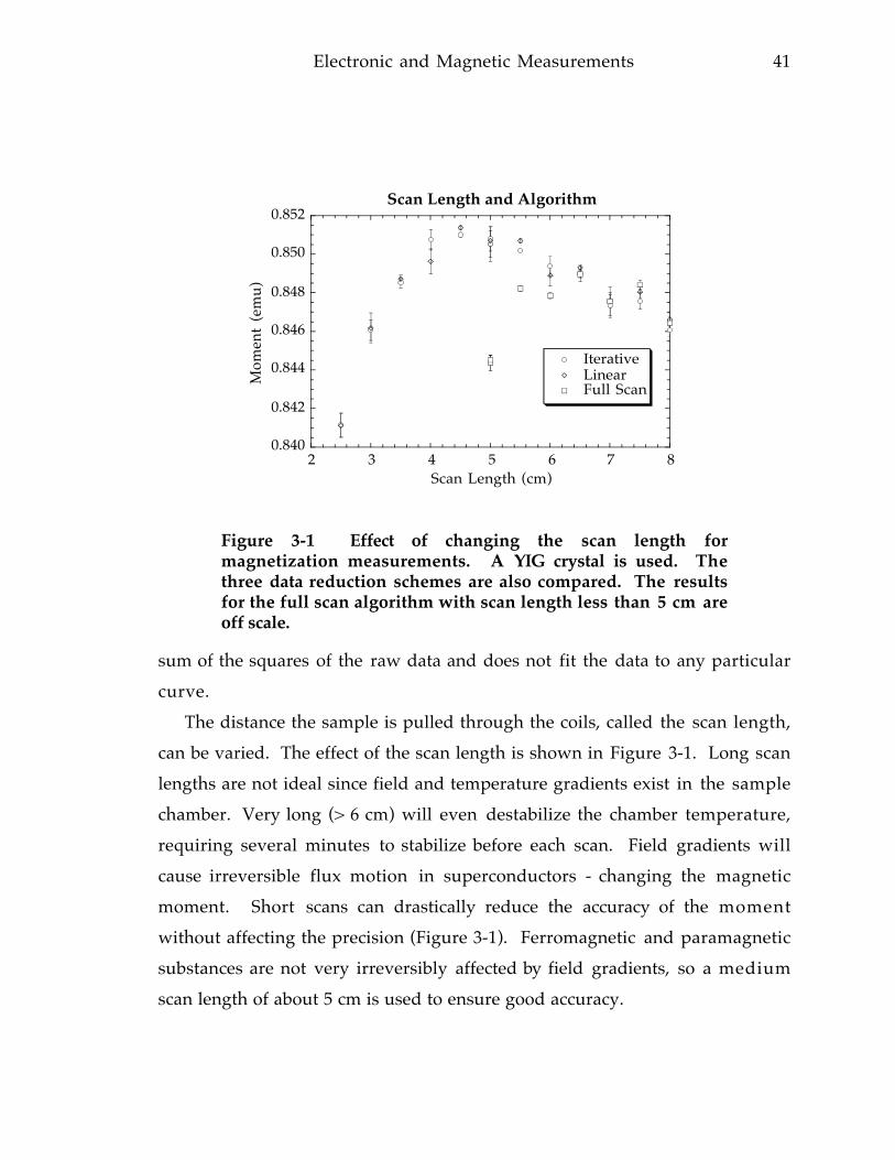
Electronic and Magnetic Measurements 41

sum of the squares of the raw data and does not fit the data to any particular

curve.

The distance the sample is pulled through the coils, called the scan length,

can be varied. The effect of the scan length is shown in Figure 3-1. Long scan

lengths are not ideal since field and temperature gradients exist in the sample

chamber. Very long (> 6 cm) will even destabilize the chamber temperature,

requiring several minutes to stabilize before each scan. Field gradients will

cause irreversible flux motion in superconductors - changing the magnetic

moment. Short scans can drastically reduce the accuracy of the moment

without affecting the precision (Figure 3-1). Ferromagnetic and paramagnetic

substances are not very irreversibly affected by field gradients, so a medium

scan length of about 5 cm is used to ensure good accuracy.

0.840

0.842

0.844

0.846

0.848

0.850

0.852

2 3 4 5 6 7 8

Scan Length and Algorithm

IterativeLinearFull Scan

Mom

ent

(em

u)

Scan Length (cm)

Figure 3-1 Effect of changing the scan length formagnetization measurements. A YIG crystal is used. Thethree data reduction schemes are also compared. The resultsfor the full scan algorithm with scan length less than 5 cm areoff scale.

42 Chapter 3

The second-derivative configuration of the SQUID coils will, in principle,

not pick up the magnetization of the sample holder if it has a uniform

magnetization. For this reason, a plastic straw with the sample wedged in the

center makes an ideal sample holder. Shrink wrap tubing, shrunk around

the sample also makes a good, but less rigid, sample holder. If string or grease

is used to hold the sample, then there will be an additional contribution to

the magnetization due to the sample holder. Similarly, if the sample is

between two quartz rods, there will be a paramagnetic contribution to the

magnetization due to the gap between the diamagnetic quartz. Materials not

containing transition elements have a diamagnetic susceptibility of about

-0.5 × 10-7 emu/g, so light sample holders (plastic) are somewhat preferable to

heavier ones (quartz glass).

The measured moment is also somewhat affected by the horizontal

centering of the sample. Rotating the sample along the field axis should have

no effect on the moment. However, it may very slightly change the

horizontal position of the sample. For whatever reason, the moment can

change a few percent with the sample rotator. Such a sensitivity on

orientation probably results in some of the unexpected jumps in the data.

The YIG sample has a moment 96.6% of that expected. Before an

experiment the sample is rotated to give the maximum moment. This is to

minimize the possible underestimation of the moment and usually provides

a region where the moment is less sensitive to small changes of the rotation.

The transverse SQUID coils can in principle also measure the net

transverse magnetic moment. A longitudinal component to the

magnetization will affect the transverse measurement. The sample can be

rotated along the axis of the sample rod, which in combination with the

transverse measurements can be used to measure the transverse-only

moment.

Electronic and Magnetic Measurements 43

3. 2. 2 AnalysisThe important quantities in magnetic measurements are the magnetic

field vector H, measured in Oersted and the magnetization intensity (or

simply the magnetization) M, measured in emu/volume (electromagnetic

unit = erg/Oersted). M is often reported in units of emu/g, emu/mole or

Bohr magnetons (µB) per magnetic atom. The magnetic induction field B

measured in gauss, defined by B = H + 4π M, is often considered more

fundamental in physics. The above units are CGS units which are more

prevalent than MKS since the equations tend to be simpler. The MKS unit

which is used commonly in the magnetic literature is the Tesla = 10000 gauss.

Most materials have a magnetization proportional to the applied field.

The magnetic susceptibility χ, defined by M = χH, relates these two quantities.

It is convenient to use χ = M/H, for non-ferromagnetic and isotropic

0.227

0.228

0.229

0.230

0.231

0.232

0.233

0.234

0 50 100 150 200 250 300 350

Sample Rotation

Mom

ent

(em

u)

Rotation Angle (°)

Figure 3-2 Magnetization of YIG sample as it is rotated alongthe field axis.

44 Chapter 3

substances. Otherwise, M = M0 + χH + χ3H3 + É can be used where χ is now a

second rank tensor describing the linear response, M0 is the spontaneous

magnetization, and χn describe the higher order nonlinear terms.

The magnetic field H can be produced either by electric currents or by the

magnetization. If a sample is magnetized, an H field is produced in the

sample to oppose the magnetization and therefore demagnetize the sample.

This demagnetization field Hd is for an ellipsoidal sample directly

proportional to the magnetization Hd = NdM, where 0 ≤ Nd ≤ 4π is the

demagnetization factor. Since the demagnetization field depends on the

shape of the sample, it is the internal field Hi = Ha - Hd the applied field minus

the demagnetization field which affects the magnetic response. Since the

correction for the demagnetization fields is often ignored, one should be wary

of the effects of demagnetization. Ferromagnets in small applied fields for

example may have reduced bulk magnetization due to demagnetization.

3. 2. 2. 1 Diamagnetism and ParamagnetismSince atoms are made up of charged particles which undergo orbital

motion and have magnetic moments, there are many ways a materials can

have a magnetic response. A diamagnetic response is that for which the

susceptibility is negative while a positive contribution to the susceptibility is

paramagnetic.

3.2.2.1.1 Larmor diamagnetism

Since the electrons in an atom are essentially free charges orbiting a

nucleus, the application of a magnetic field, by LenzÕs law, induces an

opposing magnetic moment. The resulting magnetic susceptibility is

therefore negative and known as Larmor or core-electron diamagnetism.

Both the classical and quantum mechanical analyses yield the same result,

namely that the diamagnetic susceptibility of an atom or ion is proportional

to the number of electrons it contains, Z and its cross sectional area

Electronic and Magnetic Measurements 45

χmol = -<r2>ZNAe2/6mc2 where <r2> is the mean square electron radius. Since

atomic sizes are roughly the same, and masses nearly proportional to Z, the

diamagnetic susceptibility per gram for all substances are about the same

χg ≈ -0.5 × 10-6 emu/g G. Since it is difficult to calculate <r2> accurately, it is

best to use experimental values (tabulated in [76, 77]). In most measurements

of paramagnetic and ferromagnetic substances, the diamagnetism is so small

it is usually ignored.

An example of where core diamagnetism is important is shown i n

Figure 3-3. Oxide substrates are generally diamagnetic, but provide a

significant susceptibility due to their large mass compared to the mass of a

thin film. The diamagnetism is fairly temperature independent but

substrates may contain paramagnetic impurities which alter the low

temperature diamagnetism.

-0.4

-0.3

-0.2

-0.1

0.0

0 50 100 150 200 250 300 350 400

Diamagnetic Susceptibility of Substrates

LaAlO3

Al2O

3

MgO

Susc

eptib

ility

(10

-6 e

mu/

G g

)

Temperature (K)

Figure 3-3 Diamagnetic magnetic susceptibility of typicalsubstrates. The increase in the susceptibility at lowtemperatures is due to paramagnetic impurities.

46 Chapter 3

3.2.2.1.2 Conduction electron diamagnetism

The motion of conduction electrons in a metal or semiconductor will also

provide a diamagnetic response (Landau diamagnetism) to a magnetic field.

This is difficult to calculate but generally of the same order as the Pauli

paramagnetism (section 3.2.2.1.3). A superconductor, however, expels a

magnetic field completely (Meissner effect) by the motion of the

superconducting electrons. The diamagnetism of a superconductor is,

therefore, very large, χvol = -1/4π emu/cc G in the Meissner regime. Since

superconductivity is affected by temperature and a magnetic field, the

magnetic response of a superconductor is actually quite complicated.

3.2.2.1.3 Pauli paramagnetism

Electrons in a metal can be partitioned into spin-up and spin-down bands,

parallel and antiparallel to an applied magnetic field H. The magnetic field

will lower the energy of the spin-up band compared to the spin-down band

(by 2µBH) and spin-down electrons will flip their spins and pour over into the

spin-up band. The number of electrons (per volume) that need to flip their

spins is approximately the density of electronic states, n(EF) times one half of

the energy splitting. This produces a net magnetization proportional to the

magnetic field and therefore a positive susceptibility, χvol = µB2n(EF). A more

sophisticated statistical-mechanical derivation produces the same result with

small correction proportional to T2. The Pauli susceptibility of a metal should

thus be nearly temperature independent and about the same magnitude as

the Larmor diamagnetism. Since the contribution of the Landau

diamagnetism is not known, it is usually not possible to get more than an

order-of-magnitude estimate of the Pauli susceptibility from magnetization

measurements. In principle, however, the Pauli susceptibility should be a

measure of the bare density of electronic states at the Fermi level, n(EF), in the

absence of many body effects. The linear electronic specific heat term

Electronic and Magnetic Measurements 47

(γ, section 3.3.2.1) is also proportinal to n(EF), as well as the electronic effective

mass. The ratio of these two experimental results is known as the Wilson

ratio.

3.2.2.1.4 Curie paramagnetism

If a material has unpaired electrons, their magnetic spins will be highly

susceptible to a magnetic field. The energy to orient the spins comes from the

magnetic energy MH which for an atom with effective magnetic moment p, is

µBpH. The thermal energy kBT, randomizes the spins to oppose the

alignment, so the amount of alignment is roughly proportional to µBpH/kBT.

The net magnetization is then µBp times the fraction of moments that are

aligned. So, the magnetic susceptibility of free spins should behave like

µB2p2/kBT. This is several hundred times larger at room temperature than the

core or Pauli diamagnetism/paramagnetism, and significantly temperature

dependent.

The full statistical mechanical treatment for quantum mechanical

moments with spin S, orbital angular momentum L, and total angular

momentum J, gives a magnetization per atom M = gµBJBJ(gµBJH/kBT). g is the

Land g-factor, which for atoms where J = S is the just the electron g-factor,

g = 2.00, otherwise g J L SS S L L

J J( , , )

( ) ( )

( )= + + − +

+

3

2

1

2

1 1

1.

Transition metal ions generally have their orbital angular momentum

quenched so J ≈ S. The Brillouin function, BJ(x), is defined by

B xJ

J

x J

J J

x

JJ ( ) coth( )

coth= + + −2 12

2 12

12 2

. For small x, B x xJ

JJ ( ) ≈ + 13

, while for

very large x, BJ(x) ≈ 1. The magnetization is then linear with respect to the

magnetic field until it approaches its saturation value of gµBJ. In the linear

region, µBH « kBT, the susceptibility has the Curie form χmolA B

B

N

k

g J J

T= µ +2 2

31( )

48 Chapter 3

where N

kA B

B

µ ≈2

318

emu KGauss mol

. Since the spin state is not necessarily known, the

effective moment p is often reported where p2 = g2J(J + 1). The Curie

susceptibility diverges as the temperature approaches zero; however, in real

systems the spins will Òfreeze-outÓ below some temperature making, for

example, an antiferromagnet, ferromagnet, or spin glass.

Insulators with magnetic atoms far apart (do not interact) are good

examples of Curie paramagnets. Figure 3-4 shows the magnetic properties of

an organometallic compound [SC(CH3)2C(CH3)NCH2CH2NH2]-2 FeCl with well

isolated Fe+3 ions [78]. The magnetization is slightly nonlinear at 5 K, as

predicted by the Brillouin function. The linear susceptibility can be fit to

χ = χ0 + C/T where χ0 is the diamagnetic correction (section 3.2.2.1.1). If the

0.0 100

5.0 10-3

1.0 10-2

1.5 10-2

2.0 10-2

2.5 10-2

3.0 10-2

3.5 10-2

4.0 10-2

0 50 100 150 200 250 300 350 400

Susc

epti

bilit

y (e

mu

/G

mol

)

Temperature (K)

-1.5

-1.0

-0.5

0.0

0.5

1.0

1.5

-80 -60 -40 -20 0 20 40 60 80

Mag

neti

zati

on (

µ B/

Fe)

Magnetic Field (kOe)

Figure 3-4 Paramagnetic susceptibility and hysteresis loop of aparamagnetic Fe containing organometallic compound [78].

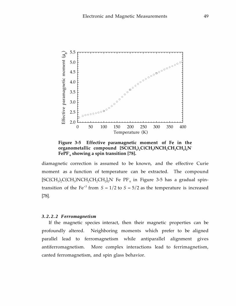
Electronic and Magnetic Measurements 49

diamagnetic correction is assumed to be known, and the effective Curie

moment as a function of temperature can be extracted. The compound

[SC(CH3)2C(CH3)NCH2CH2CH2]2N- Fe PF-

6 in Figure 3-5 has a gradual spin-

transition of the Fe+3 from S = 1/2 to S = 5/2 as the temperature is increased

[78].

3. 2. 2. 2 FerromagnetismIf the magnetic species interact, then their magnetic properties can be

profoundly altered. Neighboring moments which prefer to be aligned

parallel lead to ferromagnetism while antiparallel alignment gives

antiferromagnetism. More complex interactions lead to ferrimagnetism,

canted ferromagnetism, and spin glass behavior.

2.0

2.5

3.0

3.5

4.0

4.5

5.0

5.5

0 50 100 150 200 250 300 350 400

Eff

ecti

ve p

aram

agne

tic

mom

ent

(µB)

Temperature (K)

Figure 3-5 Effective paramagnetic moment of Fe in theorganometallic compound [SC(CH3)2C(CH3)NCH2CH2CH2]2N

-

FePF-6 showing a spin transition [78].

50 Chapter 3

3.2.2.2.1 Weiss molecular field model

The phenomena of ferromagnetism, antiferromagnetism and

ferrimagnetism can often be well described by a mean field or molecular field

model. The molecular field model simply assumes that all the interactions

from the neighboring magnetic species can be described in terms of an

effective internal or molecular field Hm, which is proportional to the magnetic

order Hm = λM (for convenience in this section, M will refer to the

magnetization per molecule). For a ferromagnet λ > 0. The total magnetic

field on an atom is then the sum of the applied field Ha and the molecular

field. Substituting Ha + Hm = H + λM for H gives a transcendental function of

M in terms of H and T which can be solved iteratively. For a simple

ferromagnet the only parameter is the molecular field constant λ, which can

be determined from the critical temperature TC via λ = 3kBTC /µB2p2.

0

10

20

30

40

50

60

70

80

160 180 200 220 240 260 280 300

Calculated 1/χ for SrRuO3

5T

5000G

5Gauss

H/

M (T

/µ B

)

Temperature (K)

Figure 3-6 Calculated inverse magnetic susceptibility ofSrRuO3 using the molecular field model.

Electronic and Magnetic Measurements 51

Above the Curie temperature the molecular field model gives the Curie-

Weiss law for the zero-field susceptibility χmolA B

B P

N

k

g J J

T= µ +

−

2 2

3

1( )

Θ, where ΘP is

the paramagnetic Curie temperature. In the Curie-Weiss molecular field

model ΘP = TC. Experimentally, for reasons discussed below, the experimental

value of ΘP is usually a slightly larger than the true critical temperature TC.

In a field, this susceptibility is slightly less than linear (χ3 < 0), like it is for

paramagnetic moments, due to saturation. The calculated inverse

susceptibility, 1/χ = H/M, is shown in Figure 3-6 for SrRuO3. The 1/χ = 0

intercept of the extrapolation of 1/χ vs. T is the paramagnetic Curie

temperature ΘP.

Below TC the mean field magnetization decreases exponentially slowly as

the temperature is raised from T = 0 K, as shown in Figure 3-7. The zero field

magnetization decreases to zero at the ferromagnetic Curie temperature TC.

Also at low temperatures, the mean field magnetic susceptibility is very

small, i.e. the application of a magnetic field increases the calculated

magnetization only slightly (Figure 3-7).

52 Chapter 3

The molecular field model assumes very little about the microscopic

origin of ferromagnetism, only that it makes sense to define a local molecular

field. Microscopic models for the interaction of atomic magnetic moments

can be formulated into a similar mean field model. In this case, the

interatomic exchange energy J can be related to the molecular field constant λ.

A microscopic model also leads to a more accurate prediction of the

magnetization. At low temperatures, the quantized moments can be

collectively excited as discussed in section 3.2.2.2.8 to give the faster decrease

in the magnetization than the molecular field model. The microscopic

model also gives a more realistic description of the observed properties near

the critical point (section 3.2.2.2.4).

0.0

0.5

1.0

1.5

2.0

0 50 100 150 200

Calculated Mean Field Magnetization for SrRuO3

5T5kOe5 Oe

Mag

neti

zati

on (

µ B)

Temperature (K)

1.985

1.990

1.995

2.000

2.005

0 20 40 60 80 100

Mean Field Forced Magnetization

5K50K

Mag

neti

zati

on (

µ B)

Magnetic Field (kOe)

Figure 3-7 Mean field magnetization calculated in variousfields for SrRuO3 with TC = 165K. Inset show the very smallfield dependence of the magnetization (forced magnetization)in this model.

Electronic and Magnetic Measurements 53

3.2.2.2.2 Itinerant electron Model

The ground state properties of a metallic ferromagnet are believed to be

fairly well described by the band theory which has advanced in the recent

decades [79]. The thermal excitations and finite temperature properties,

however, are more difficult because of the effects of strong electron-electron

correlations in narrow energy bands. This limits the utility of traditional

Hartree-Fock or mean field theory described briefly in this section and

requires a treatment of generalized spin density fluctuations described i n

section 3.2.2.2.3 to describe fully the magnetic excitations in itinerant electron

ferromagnets.

The quantum mechanical exchange interaction can lead to

ferromagnetism in an electron gas within the band model, commonly known

as Stoner ferromagnetism [80, 81] or itinerant electron ferromagnetism.

Using the molecular field approximation, a ferromagnetic state is realized for

Jn(EF) > 1 where J is the average intra-atomic exchange energy per atom and

n(EF) is the density of states at the Fermi level. This is also known as the

Stoner condition for ferromagnetism. For Jn(EF) < 1 the material is not

ferromagnetic but has a Pauli susceptibility enhanced by 1/(1-Jn(EF)) [82]. This

factor is called the Stoner enhancement factor.

The effect of the magnetization at finite temperatures can be calculated

using the mean field approximation. Specifically, the energy of the up (down)

spin band is uniformly lowered (raised) by an amount proportional to the

magnetic polarization ζ and a molecular field constant. Since this model

assumes electrons are either in up or down spin bands, the excitations are

known as single particle, spin flip, or Stoner excitations. There is no energy

gap required for Stoner excitations. However, zero or low energy excitations

require a non-zero momentum transfer, while excitations with zero

momentum transfer require an excitation energy equal to the exchange

splitting as can be seen in Figure 3-8. The region of allowed Stoner excitations

54 Chapter 3

is called the Stoner continuum. Collective, spin-wave excitations are not (yet)

included. The mean field analysis [81] gives (M/M(0,0))2 = 1-(T/TC)2 +

2χ(0,0)H/M.

As expected from a Ginzberg-Landau/mean-field approximation section

3.2.2.2.5, this formula predicts mean field exponents of β = 1/2 and γ = γ ′ = 1

for T near TC, and linear M2 vs. H/M Arrott plots. Above TC the inverse

susceptibility is proportional to T2-TC2 [81], which is in gross disagreement

with the experimentally observed Curie-Weiss law (1/χ = T - TC). The finite

zero field susceptibility at T = 0, χ(0,0), is essentially the enhanced Pauli-

susceptibility [83].

Unlike the local moment model which requires the zero temperature

saturation moment M(0,0) to be equal to the sum of all the moments, the

band model allows for opposing moments in the minority band at T = 0 (ζ<1).

This has been used to explain the low saturation moments in metallic

ferromagnets, particularly when the saturation moment is lower than the

effective Curie-Weiss moment. The Rhodes-Wohlfarth ratio peff/psat is used

to estimate the itinerant electron magnetism character of a material. A plot of

peff/psat vs. TC, known as the Rhodes-Wohlfarth plot, shows that the

likelihood of a large peff/psat decreases as TC increases [84].

The magnetization in zero field decreases as M(0,0) √(1-(T/TC)2) which has

a slightly stronger temperature dependence than the common approximation

M/M(0,0) = 1 - (T/TC)2/2. This T2 dependence on the magnetization is often

attributed to Stoner, or single particle excitations.

The specific heat at low temperatures is dominated by a linear term,

Cv = γT. The predicted specific heat discontinuity at TC is too small to be

consistent with the observations [84].

Spin wave excitations can also be included within this simplified band

model and predicts the T3/2 temperature dependence described previously for

Electronic and Magnetic Measurements 55

T/TC « ζ2 (fractional polarization)[81]. A more complete improvement of the

Stoner theory takes into account the effect of spin density fluctuations. Such

improvements are discussed the following section.

3.2.2.2.3 Generalized Model

The self-consistent-renormalization (SCR) theory [79, 84, 85] combines

both single particle and spin wave excitations into generalized interacting

spin density fluctuations. It deals with the coupled modes of spatially

extended spin density fluctuations in a self-consistent fashion. The theory

gives a new mechanism for the Curie-Weiss magnetic susceptibility

associated with the spatially extended modes of spin fluctuations instead of

the local moments as spatially localized spin fluctuations. Furthermore, the

theory is successful quantitatively in explaining various physical properties of

weak itinerant ferro- and antiferromagnets: the theory contains a limited

number of parameters which can be determined experimentally. Thus by the

1970Õs the theory of magnetism was advanced to the stage of having two

established regimes in the opposite extremes, the local moment systems and

weak itinerant ferro- and antiferromagnets. In the former regime the spin

fluctuations are localized in real space while in the latter they are localized i n

k-space. In order to unify the two extremes into a single theory an

interpolation theory for the intermediate regime was developed in the 1980Õs

using the functional integral method within the static approximation.

56 Chapter 3

The theory predicts that spin waves exist only in a small region at the

origin of (ω,k) space with dispersion relation ω = k2D, where D is the spin

wave stiffness. The strongest intensity of the dynamical susceptibility is i n

the region where the spin wave excitations meet the Stoner continuum

shown in Figure 3-8. In the low temperature limit a T3/2 law is predicted i n

the magnetization. However, calculations for Ni3Al [86] show that the

magnetization is best approximated by a T2 dependence over a broad

temperature range below TC. It has been assumed that in the highly

correlated limit, i.e. metallic ferromagnets with a large saturation moment,

the magnetization will obey the spin wave T3/2 law [85], presumably because

of strong evidence for the existence of spin waves in metallic ferromagnets.

SpinWaves

StonerContinuum

Ene

rgy

Momentum Transfer

Magnetic Excitation Spectrum

Figure 3-8 Energy spectrum of magnetic excitations. Spinwave excitations have a one-to-one dispersion relation whileexcitations in the Stoner continuum (shaded region) do not.The intensity of excitations in the Stoner continuum isstrongest where the spin waves meet the continuum.

Electronic and Magnetic Measurements 57

The major advancement of the SCR theory is the development of a new

mechanism for the Curie-Weiss magnetic susceptibility applicable to itinerant

electron ferromagnets. The paramagnetic Curie-Weiss susceptibility arises

essentially from the opposition of the magnetic energy to order the spins and

the thermal energy to disorder them. The magnetization is then proportional

to µBH/kBT, giving the inverse susceptibility H/M linear in T. In the case of

the weak itinerant electron ferromagnets there are no localized spins above

TC so the susceptibility cannot arise from this mechanism. Instead, the

changing mean-square local amplitude of the spin fluctuation provides the

Curie-Weiss susceptibility.

The SCR expression for the inverse magnetic susceptibility contains a

contribution from the mean-square local amplitude of the spin fluctuation SL2

[84] which can be derived from the fluctuation-dissipation theorem.

Calculations have shown that SL2 increases almost linearly with temperature

above TC giving rise to the Curie-Weiss law. This is in contrast with the local

moment mechanism where SL2 is a constant. The Curie constant of the new

mechanism is related to the band structure around the Fermi surface and is

independent of the saturation moment at T = 0. This Curie-Weiss law should

hold even for paramagnetic metals when they are very close to the

ferromagnetic instability, in contrast to that predicted by paramagnon theories

[84].

The temperature variation of SL2(T), which determines the new Curie-

Weiss mechanism is strongest when the stiffness of the longitudinal spin

fluctuations is small. When the longitudinal stiffness is small, a relatively

rapid increase in SL2(T) with inverse temperature is expected above TC and it

should saturate at a certain value determined by the band structure. After

saturation the spin fluctuations behave like local moments with a certain

degree of short range order, since the local amplitude of the spin density is

almost fixed. This phenomenon is called temperature-induced local

58 Chapter 3

moments [84]. Thus, a subtle change is expected in the Curie-Weiss

mechanism at some temperature above TC. This has been used to explain the

change in the Curie constant at around 3TC in Co(S/Se)2 [87]. This

phenomenon is also expected in some exchange-enhanced paramagnets.

In Heusler Alloys such as Pd2MnSn, Ni2MnSn, Cu2MnAl, etc., manganese

atoms are spatially well separated from each other (> 4Å), and are believed to

carry well-defined local moments since the Rhodes-Wohlfarth ratio is close to

one and neutron scattering experiments can be well analyzed with the

Heisenberg model. The ferromagnetic MnPt3, FePd3 and antiferromagnetic

FePt3 are likely to have well-defined 3d local moments that couple with

itinerant 4d or 5d electrons of Pd or Pt. CoS2 and the metallic ferromagnets

AMnO3 described in chapter 4 fit perhaps best in this category.

In the intermediate regime between the local moment ferromagnets and

the weak itinerant-electron ferromagnets are the Ferromagnetic transition

metals (Fe, Co, and Ni) and compounds Fe3Pt and CeFe2. These materials

have relatively high TC’s but have Rhodes-Wohlfarth ratios [84, 88] greater

than one. The ferromagnetic oxide SrRuO3 also fits in this category as

described in detail in Appendix A.

MnSi is a good example of a weak-ferromagnetic helimagnet which is well

described by the SCR theory. Other weak ferromagnets such as Ni3Al, ZrZn2

and Sc3In can also be described in terms of the SCR theory [84].

Metallic Cr which orders antiferromagnetically below 312K with a long

period spin density wave, is the most often used example of an itinerant

electron antiferromagnet. However, the Curie-Weiss law is not obeyed above

TN. The magnetism of Cr is best described with an itinerant electron approach

with the addition of a nesting Fermi surface model to describe the spin

density waves [84]. The antiferromagnetic metals γ-Mn, γ-(FeMn) and γ-Fe

have also been studied [84].

Electronic and Magnetic Measurements 59

Examples of nearly ferro- or antiferromagnetic metals which show a large

susceptibility are CoSe2 (Curie Weiss) Pd or YCo2 [84], and V2O3 [89]. The

nearly ferro- or antiferromagnetic semiconductor FeSi (Curie Weiss) shows a

Curie-Weiss susceptibility above 700K with a broad transition at 500K to a low

susceptibility state [84].

3.2.2.2.4 Critical region

As the temperature approaches the critical temperature TC, the

spontaneous magnetization vanishes and the susceptibility diverges. This

makes these properteis not analytic near TC. The observed properties are well

described by a power law |T - TC|n where n is a scaling exponent. For

example, the spontaneous magnetization varies as (TC -T)β for T < TC, while

the susceptibility varies as (TC - T)γ for T > TC, and for T = TC (critical isotherm)

Mδ = H. The scaling exponents in the critical region are called critical

exponents.

The critical exponents are very similar for a wide range of second order

phase transitions. They tend to depend only on the general form of the

interaction causing the phase transition, such as the dimensionality, and not

on the particular material. Thus most ferromagnets fall into the universality

class of 3-dimentional Heisenberg or Ising ferromagnets. The theoretical

critical exponents calculated for these models is given in Table 3-1. There are

only two unique critical exponents in each universality class. The others are

related via the scaling relations such as γ = β(δ -1).

According to the scaling hypothesis [90], the magnetic equation of state i n

the critical region depends only on the scaled variables H/|TC/T - 1|β+γ and

M/|TC/T - 1|β. For example, a plot of the scaled M2 vs. the scaled H/M, (scaled

60 Chapter 3

Arrott plot), will then have only two curves: one branch for the T < TC data

and another for T > TC.

The magnetization near TC is predicted in the SCR theory, described i n

section 3.2.2.2.3, to behave as M = (TC4/3-T4/3)1/2 [84, 91] which reducecs to β = 1

for T near TC.

Table 3-1 Theoretical 3-dimentional critical exponents fordifferent models and selected experimental values [92, 93].

β γ δIsing .33 1.24 4.8Heisenberg .36 1.39 4.8Mean Field .5 1 3

ZrZn2 .50(3) 1.02(5) 3.1(3)Fe, Ni, YIG .37(2) 1.2(2) 4(1)

3.2.2.2.5 Landau mean field theory

Near the critical temperature TC the molecular field, or mean field model

(section 3.2.2.2.5) predicts mean field critical exponents (Table 3-1). The

Landau theory of continuous, second order phase transitions (excluding

fluctuations) arrives at the same mean field result. Here the free energy is

expanded in a Taylor series of the order parameter (M in the case of

ferromagnetism). Due to the symmetry of the order parameter, only even

powers of M are nonzero. The first few terms are [94]: G = G0 + a(T - TC)M2 +

bM4 - HM. At a given H and T, M can be found by minimizing the free energy

G. The general solution is H/M = 2a(T - TC) + 4bM2. Below TC the saturation

magnetization (H = 0) is found to be M2 = (TC - T)a/2b, giving the critical

exponent β = 1/2. Above TC in a field, M is small so the bM4 term can be

ignored. This gives a susceptibility χ = M/H = (T - TC)-1/2a, and a critical

Electronic and Magnetic Measurements 61

exponent γ = 1. Along the critical isotherm T = TC, H = 4bM3 so the critical

exponent δ = 3.

3.2.2.2.6 Arrott Plot

According to the Landau equation of state H/M = 2a(T - TC) + 4bM2, a plot

of M2 vs. H/M at a constant temperature gives a straight line. At TC, this line

intersects the origin. The M2 = 0 intercept gives the inverse susceptibility

1/χ0 (H = 0) while the H/M intercept gives the spontaneous magnetization

M02 (H = 0).

In real systems near the critical point, non mean field critical exponents

are observed. Thus the plot of M2 vs. H/M (Arrott plot) will not necessarily

be straight lines, but allows a visual analysis of the data [94]. The TC

determined from the Arrott plot is the isotherm that extrapolates to the

origin. Likewise, the extrapolation to the axis intercepts give the H = 0

spontaneous magnetization M0 (T < TC) and inverse susceptibility

1/χ0 (T > TC) and allows a visual exstimation of the error. From these M0(T)

and χ0(T) the critical exponents β and γ can be estimated by fitting

M0(T) ∝ (1 - T/TC)β and χ0(T) ∝ (T/TC - 1)-γ.

If the assumption of scaling is incorrect, such as a crossover from one

scaling region to another as the temperature changes, then the entire data will

not scale with the same exponents. In this case, the method described above

is better for characterizing the separate regions. Such a crossover is observed

in SrRuO3 where β appears to change from 0.32 to 0.38 (Appendix A) so that

the entire data does not scale very well with a single average value for β.

3.2.2.2.7 The Curie temperature

Because the Curie temperature affects many of the properties, there are

several ways of measuring it. One of the simplest is finding the paramagnetic

62 Chapter 3

Curie temperature, the temperature where the linear extrapolation of the 1/χ

curve crosses 1/χ = 0. Near the critical temperature however, 1/χ is not

necessarily linear in T since 1/χ = (T - TC )γ where γ is usually large than 1.

Thus the paramagnetic Curie temperature is usually slightly larger than the

true critical temperature.

In principle the thermodynamic critical temperature can be found by

fitting the divergence of all the measured quantities and using the scaling

relations. This assumes a true critical region has been reached where the

critical exponents do not change. The simpler method using the Arrot plots,

described in the previous section (3.2.2.2.6) can give as accurate results. Thus,

the Arrott TC is probably the best simple way of finding the critical

temperature.

The most basic definition of TC for a ferromagnet is the temperature where

the spontaneous magnetization drops to zero (as the temperature is raised).

Unfortunately due to demagnetization effects, the zero applied field

magnetization will drop to zero at TC faster and less uniformly than expected.

Nevertheless, the temperature where the magnetization, measured in zero or

small applied field, is often used to measure the critical temperature and is

called here the remnant TC.

In an applied field, the magnetization does not drop to zero because of the

large susceptibility near TC. However, below TC the magnetization has a

negative curvature while above TC it has a positive curvature. Thus the

inflection point of the M vs. T curve (denoted here as the inflection TC) is

often used to measure the Curie temperature. In the mean field model, the

inflection TC is quite close to the real critical temperature. Figure 3-7 shows

the calculated M vs. T of SrRuO3 in various fields. In a 5 T applied field, the

inflection point is 1.6 K higher than the true TC used for the calculation. This

agrees well with the experimental data shown in Figure 3-9, where the

Electronic and Magnetic Measurements 63

derivatives are calculated numerically from the measured magnetization. In

some systems, the inflection TC can increase substantially as the applied field

is increased, as seen for Gd0.67Ca0.33MnO3 in section 5.1.4, making it a poor

estimate of the Curie temperature.

0.0

0.2

0.4

0.6

0.8

1.0

140 150 160 170 180 190

SrRuO3 Inflection T

C

5.5T3T1T5kOe1kOe300 Oe50 Oe

Mag

neti

zati

on (

µ B)

Temperature (K)

167 K

163 K

166 K

164 K

Figure 3-9 The inflection TC measured for a SrRuO3 pellet.For H < 1 Tesla the inflection TC is within 1 K of the Arrott TC

= 163 K. At higher H the inflection TC increases by only a fewdegrees.

3.2.2.2.8 Spin waves

Collective excitations (spin waves) are expected to be the dominant mode

of excitations at the lowest temperatures. This is because it can be shown that

collective excitations will always have lower energy than single spin

excitations. The spin wave theory has been mostly developed for localized

moments [95] but can also be generalized to include k-space electrons [81].

64 Chapter 3

The energy ω of a spin wave is given by ω = Dk2 + ∆ for low momentum k

spin waves. D is the spin wave stiffness and ∆ is a gap energy arising from

anisotropy or applied magnetic fields. With no gap the spontaneous

magnetization decreases as T3/2 [95]: M(T)/M0 = 1 - (T/Θ3/2)3/2. For a

ferromagnet with spin S and spin density n, Θ3 2 2 612

423

/ .=

πnS D

kB

. The

specific heat of these excitations [95] also follows a T3/2 law:

cV = 1.925 kBnS(T/Θ3/2)3/2. The spin wave stiffness D may be estimated from

the critical temperature TC and number of near neighbors z, using D = 2JS5/3

and kB TC /J = 0.0521(z - 1)(11S(S + 1)-1) [96], where J is the exchange energy.

0.0

0.1

0.2

0.3

0.4

0.5

0.6

0.7

0 2 4 6 8 10

Cor

rect

ion

fact

or M

(t)

kBT/gµ

BH

0.00

0.050.10

0.150.20

0.25

0.300.35

0.0 0.5 1.0 1.5 2.0

Figure 3-10 Correction factor to the T3/2 contribution of themagnetization in the spin wave theory due to a magnetic fieldH.

The first order effect of a magnetic field providing a gap ∆ = gµBH /kBT, is

to adjust the T3/2 coefficient by a function of kBT/gµBH: M(T)/M0 =

1 - F3/2(kBT/gµBH)/ζ(3/2) (T/Θ3/2)3/2. This correction factor M(t), shown i n

Electronic and Magnetic Measurements 65

Figure 3-10, depends on the temperature T, thus altering the temperature

dependence of the magnetization to have an effective power higher than 3/2

[97]. The Bose-Einstein integral function [95] FP(x) is given by FP(x) = e

n

n x

Pn

−

=

∞

∑/

1

and ζ(P) = 1

1 nPn=

∞

∑ (e.g. ζ(3/2) = 2.612 and ζ(1/2) = -1.460). The correction C(t) to

the T3/2 contribution to the heat capacity is similar: C(t) = [F5/2(t) + 4F3/2(t)/5t +

4F1/2(t)/15t2)]/ζ(5/2), where t = kBT/gµBH. The correction factor C(t) is shown

in Figure 3-11. Due to the Maxwell relation the increase in the effective

power in M(T) also increases the effective power of dc/dH (T).

Figure 3-11 Correction factor to the T3/2 contribution of theheat capacity in the spin wave theory due to a magnetic fieldH.

0.0

0.2

0.4

0.6

0.8

1.0

0 2 4 6 8 10

Cor

rect

ion

Fact

or C

(t)

kBT/gµ

BH

0.0

0.2

0.4

0.6

0.8

1.0

0.0 0.5 1.0 1.5 2.0

66 Chapter 3

3.2.2.2.9 Irreversibility

Below TC, a ferromagnet must undergo a first order phase transition when

the field direction is changed. Like all first order processes, this involves

nucleation and growth (of magnetic domains) and can be hysteretic.

Technically there is only hysteresis when the internal field changes sign; if

the field increases or decreases while retaining the same sign (direction), the

change in the magnetization is continuous. However, in real systems, there

exist internal anisotropy and demagnetization fields. So in low fields

irreversible behavior can be found.

Figure 3-12 SrRuO3 showing spin-glass like irreversibility ofzero-field-cooled and field-cooled measurements in a smallfield. The field cooled curve may look saturated, but isactually less than 1/10 saturated at low temperatures. A smallpeak is observed in the zero-field-cooled measurement whenthe reversibility point is reached.

The field required to reduce to zero the magnetization of a saturated

sample, is called the coercive field. When the coercive field is large, such as

0.00

0.02

0.04

0.06

0.08

0.10

0.12

0 50 100 150 200

SrRuO3 Pellet irreversibility

FCZFC

Mag

neti

zati

on (

µ B)

Temperature (K)

Field Cooled

Zero Field Cooled

20 Oersted Magnetization

Electronic and Magnetic Measurements 67

in polycrystalline SrRuO3, the irreversibility will be evident in many

measurements. The coercivity depends on the microstructure of the sample,

and therefore depends on the processing. SrRuO3 single crystal for instance

(Appendix A) has a coercive field 100 times smaller than polycrystalline

SrRuO3.

0.0

0.2

0.4

0.6

0.8

0 1000 2000 3000 4000 5000

SrRuO3 initial magnetization

Mag

neti

zati

on (

µ B)

Magnetic Field (Gauss)

Inflection Point

Figure 3-13 Initial magnetization of SrRuO3 pellet at 5 K, aftercooling in zero field. The magnetization follows a “S” shapedcurve providing an inflection point.

In the irreversible regime, a ferromagnet will have magnetic properties

similar to that of a spin glass [98]. For example, it is common to characterize

spin glasses [99] (or disordered superconductors) by comparing the field-cooled

(sample cooled below TC in the measuring field) and zero-field-cooled

(sample cooled in zero field and then the field applied before measuring upon

warming) magnetization in a small field. For a spin-glass or disordered

superconductor, these two curves are different. In such small fields, a

68 Chapter 3

ferromagnet will also show such hysteresis, as demonstrated in Figure 3-12

for SrRuO3. The field cooled curve may look like a ferromagnetic M vs. T

curve, however it is influenced greatly by the demagnetization field and

coercivity. For example in applied fields lower than the maximum

demagnetization field (4πNMS) the net magnetization can only increase until

the demagnetization field cancels the applied field (M = H/4πN). The a plot

of M vs. T in this case will show a constant, low value for M, until the true

magnetization decreases near TC (see for example the low field data in [29]).

Another characteristic of a spin glass is an “S” shaped magnetization

curve, which gives an inflection point in M vs. H. Such a curve is also

observed for a ferromagnet, such as that seen for SrRuO3 in Figure 3-13. The

curves for increasing and decreasing fields will meet at the irreversibility

point. The irreversibility points measured by the two methods (constant T,

10

100

1000

10000

100000

0.01 0.1 1

SrRuO3 Irreversibility Line

Hrev (const T)Hrev (Const H)

Rev

ersi

ble

Fiel

d (

Hre

v)

(Gau

ss)

1-T/Tc

Hrev

= (1-T/TC)1.5

Figure 3-14 Magnetic irreversibility line for polycrystallineSrRuO3. Above the line the magnetization is reversible,below it is irreversible. The irreversibility exponent is about1.5.

Electronic and Magnetic Measurements 69

Figure 3-13; and constant H, Figure 3-12) give an irreversibility line, much

like that in superconductors. For polycrystalline SrRuO3 the reversible field is

approximately proportional to (1 - T/TC)1.5.

Like many glassy systems, the magnetic properties in the irreversible

region are time dependent. In a ferromagnet the domain walls are pinned

and so must overcome some barrier energy to move. Thus the

magnetization increases in a time dependent manner. Figure 3-15 shows the

magnetization of a SrRuO3 pellet at 5 K after increasing the magnetic field

from 0 Gauss (where the magnetization was 0.0076 µB) to 100 Gauss. The

magnetization increases with a Log(time) dependence, with 98% of the

increase happening before the first data point (about 1 minute). Such a

logarithmic time dependence is also characteristic of a spin glass [99].

SrRuO3 has all the properties of a ferromagnet, and because of this long

range order can not be a spin glass. The domain structure of a ferromagnet

provides magnetic disorder on a larger length scale than a spin glass, but to be

a spin glass, the disorder must be on the atomic scale.

3. 2. 2. 3 AntiferromagnetismIn an antiferromagnetic substance, the neighboring magnetic moments

align antiparallel. Such a material is called an antiferromagnet. In the

ordered state, there is often no net moment in zero field. Thus magnetization

measurements cannot easily measure the magnetic order. In neutron

diffraction, the magnetic unit cell multiplies giving extra diffraction peaks.

The intensity of these peaks is a direct measure of the ordering.

In a magnetic field, an antiferromagnet has a small positive susceptibility.

Above the ordering temperature, or Néel temperature TN, the susceptibility

can be well described by the Curie-Weiss law used for ferromagnets. Since the

interactions are antiparallel, the coupling is of the opposite sign as that for a

70 Chapter 3

ferromagnet. This leads to a negative paramagnetic Curie temperature

ΘP ≈ -TN, where the susceptibility above TN is given by χmolA B

B P

N

k

g J J

T= µ +

−

2 2

3

1( )

Θ.

Below the ordering temperature TN, M vs. H is still linear with no H = 0

magnetization, but the susceptibility depends on the orientation of the

magnetic field with respect to that of the magnetic moments [56]. For

example, Figure 3-16 shows the susceptibility of platinum containing

“CaRuO3” crystals, or CaRu/PtO3 described in section 2.1.2.1. If the magnetic

field is applied parallel to the ordered moments, the applied torque (µ × H) is

small so the susceptibility decreases to zero. The CaRu/PtO3 crystal when

oriented with the 2-fold symmetric axis parallel to H shows such a

susceptibility. When the field is perpendicular to the ordered moments, the

torque is maximized providing a large, constant susceptibility in the ordered

0.01620

0.01625

0.01630

0.01635

0.01640

0.01645

100 1000 10000

Magnetization CreepM

agne

tiza

tion

(µ B

)

Time (s)

Figure 3-15 Time dependent magnetization of SrRuO3 pelletat 5 K. The field was increased from 0 to 100 Gauss. Themagnetization follows a Log(time) dependence.

Electronic and Magnetic Measurements 71

state. This is seen in the crystals oriented with a 3-fold symmetric axis parallel

to H. Without Pt, CaRuO3 has an antiferromagnetic like susceptibility

(1/(T + ΘP)) above 50K (ΘP ≈ -210K peff ≈ 9.75 or S ≈ 1.14) but does not become

antiferromagnetic. Instead, it remains paramagnetic but with a stronger

temperature dependence ≈ 1/T (Figure 3-16). From 2 K to 20 K the

susceptibility fits well to (1/(T + ΘP)) with an antiferromagnetic slope

(ΘP = -73K peff = 4.17 or S = 0.64).

3. 2. 2. 4 FerrimagnetismIf the sublattices of different moment orientation do not exactly cancel,

there is then a small ferromagnetic moment in the ordered state, that behaves

5.0 10-6

1.0 10-5

1.5 10-5

2.0 10-5

2.5 10-5

3.0 10-5

3.5 10-5

4.0 10-5

0 50 100 150 200 250 300 350 400

CaRuO3 and Pt Containing CaRuO

3 Crystal

CaRuO3

3-fold axis crystal2-fold axis crystal

χ (e

mu/

g/G

)

Temperature (K)

Figure 3-16 Magnetic susceptibility of a Pt containing“CaRuO3” crystal. The crystal was aligned with its 2-foldsymmetric axis parallel to the applied field has a susceptibilitycharacteristic of antiferromagnetic moments aligning parallelto the field, while the 3-fold axis appears to have momentsperpendicular to the field.

72 Chapter 3

with temperature and field much like a ferromagnet. When this is due to a

canting of neighboring moments from truly parallel or antiparallel, this is

called a canted antiferromagnet. If the ferromagnetic moment is not due

entirely to canting but arises from the different strengths of the sublattice

magnetizations, the material is called a ferrimagnet.

Most commercial insulating “ferromagnets” are actually ferrimagnets.

Common examples are ferrites and garnets such as YIG. The multiple

magnetic interactions inherent to a ferrimagnet provide a variety a magnetic

behavior. For example, when the magnetizations of the opposing sublattices

exactly cancel, the net moment is zero like it is in an antiferromagnet. The

temperature where this occurs is called the compensation temperature TComp.

3.2.2.4.1 Mean field model for Gd0.67Ca0.33MnO3

The gross features of a ferrimagnet can be explained using the molecular

field model of section 3.2.2.2.5. For a ferrimagnet with two sublattices, the

total magnetization M is the sum of the two sublattice magnetizations MA and

MB. The molecular field acting on each sublattice can then arise from

interactions with atoms in the other sublattice as well as atoms in the same

sublattice. For example on the A sublattice HmA = λAAMA + λABMB. The

molecular field constants λ ij can be either positive for ferromagnetic coupling

between sublattices or negative for antiferromagnetic coupling. For a

ferrimagnet or antiferromagnet, there must be strong antiferromagnetic

coupling. Similarly, on the B sublattice HmB = λBBMB + λABMA. Once the

molecular field constants are known, the magnetization of each sublattice can

be calculated iteratively as described in section 3.2.2.2.5 until self consistency is

reached.

Electronic and Magnetic Measurements 73

Gd0.7Ca0.3MnO3Hwang et al.

Figure 3-17 Temperature - tolerance factor phase diagramfrom reference [100], with the position of Gd0.67Ca0.33MnO3

indicated.

This has been done for Gd0.67Ca0.33MnO3 where the experimental results

are given in chapter 5. In Gd0.67Ca0.33MnO3 the Mn atoms are on one

sublattice (B) and Gd atoms on the other (A). The dominant molecular field

constant is expected to be the ferromagnetic Mn-Mn coupling due to the

stronger 3d exchange interaction. From the trend found in the manganese

ferromagnetic ordering temperature as a function of the average of the R and

A atom size [100] in R1-xAxMnO3, shown in Figure 3-17, the TC is expected to be

around 60K. The molecular field constant can then be approximated using

the relationship found for a ferromagnet in section 3.2.2.2.5, namely

λBB = 3kBTC /µB2pB

2.

Here pi2 also includes the site occupancy for each type of atom on the i

sublattice. For Gd0.67Ca0.33MnO3, the Mn (B) sublattice has two magnetic

contributions since the site is 67% occupied by Mn+3 (S = 2) and 33% occupied

74 Chapter 3

by Mn+4 (S = 3/2). This gives pB2 = Σ nig

2si(si +1) = 21. On the Gd/Ca (A)

sublattice, only Gd+3 (67% occupied, S = 7/2) has a moment giving pA2 = 42.

The Gd-Gd interaction is expected to be negligible, and therefore λAA ≈ 0,

since the Gd 4f electrons are well localized. The Gd atoms are expected to

order due to the significant Gd-Mn interaction which is antiferromagnetic, so

λBA < 0. In the case of Gd0.67Ca0.33MnO3, there exists a temperature where the

magnetization of the larger, but poorly ordered, Gd moments exactly cancels

that of the Mn sublattice. This temperature is called the compensation

temperature TComp.

The compensation temperature TComp can be used to estimate the

molecular field constant λBA. The weakly coupled Gd approximately act like

free paramagnetic spins reacting to the internal (molecular) field caused by

the ordered Mn moments. In zero applied field this gives

MA = HmA µB2pA

2/3kBT. The internal field on the A sublattice is related to λBA

from HmA = λBAMB. At T = TComp, there is no net magnetization so MB + MA = 0.

Combining these relations gives λBA = -3kBTComp/µB2pA

2.

Above TN, the susceptibility can be calculated analytically [101] giving a

hyperbola for 1/χ vs. T shown in Figure 5-5. The high temperature asymptote

is a straight, Curie-Weiss like, line which intersects the T axis at

ΘP = (µB2/3kB) (pB

4λBB + 2pB2pA

2λBA)/(pB2 + pA

2). For Gd0.67Ca0.33MnO3, λBA < 0 and

λBB > |λBA| so ΘP should be less than but close to 7λBB (µB2/3kB) which is 1/3 of

the value that would be expected (TC of Mn) if no Gd moments were present.

In this model, the ferrimagnetic Néel temperature is given by

TN = pB2λBB (µB

2/3kB)[1/2 + √(1/4 + (pAλBA/pBλBB)2)] [101]. For λBB > |λBA| this is

only slightly greater than the TC = pB2λBB (µB

2/3kB) expected if the Gd moments

were absent. Combining this result with that of the last paragraph gives a

Electronic and Magnetic Measurements 75

general requirement of this model TN/ΘP > (pB2 + pA

2)/pB2 = 3, which should be

easily verified from experiments (section 5.1.5.1).

0

0.2

0.4

0.6

0.8

1

1.2

0 2000 4000 6000 8000 10000 12000

Calculated Gd0.67

Ca0.33

MnO3 Arrott Plot

8083K85K

Mag

neti

zati

on2 (

µ B/

mol

e)2

H/M (Oe/µB

)

Figure 3-18 Calculated Arrott Plot for Gd0.67Ca0.33MnO3 usingthe mean field model with TC = 83.3 K.

The critical temperature TC, of a ferrimagnet is the Néel temperature TN.

As T approaches TN from below, the zero field magnetization vanishes much

like that of a ferromagnet. The theoretical Arrott plot TC (shown in Figure 3-

18) is equivalent to the remnant TC = TN. The mean field calculation gives a

nearly linear critical isotherm on the Arrott plot, shown in Figure 3-18, since

Mδ = H and δ = 3 is the mean field critical exponent. The inflection point i n

the M vs.. T curve is also a good estimate of TC. In this model, the inflection

TC increases by only 0.55 K/Tesla as H is increased.

Below TC the calculated magnetic susceptibility is small since the internal

molecular field is quite large. The ferrimagnet susceptibility calculated here,

however, is not uniformly decreasing as T decreases like it does for a

76 Chapter 3

ferromagnet. Instead, it peaks as shown in Figure 3-19 near the compensation

temperature TComp.

0

0.1

0.2

0.3

0.4

0.5

0 20 40 60 80 100

Calculated Susceptibility of Gd0.67

Ca0.33

MnO3

Susc

epti

bilit

y (µ

B/

T)

Temperature (K)

χ = (M(6T) - M(4T))/2T

Figure 3-19 High field differential susceptibility forGd0.67Ca0.33MnO3 calculated using the mean field model. Themaximum is at 11.5 K which is near TComp = 14.2 K in thismodel.

3.3 Heat CapacityThe heat capacity of a sample, particularly at low temperatures, is a

powerful experimental technique which gives fundamental information

about low-lying excitations of many kinds (phonons, electrons, magnons,

etc.). Microscopic models which describe these excitations typically give

quantitative predictions of the specific heat which can then be used to check

the theory. The has been quite successful at low temperatures where the

excitations are simple. At higher temperatures, the dispersion relation of the

excitation spectrum can become less simple and therefore complicate the heat

Electronic and Magnetic Measurements 77

capacity. Thermal measurements at higher temperatures T>100K are typically

only used to study phase transitions.

3. 3. 1 MeasurementThe most straightforward method of measuring heat capacity is adiabatic

calorimetry. Here, the heat capacity C=∆Q/∆T is measured directly by applying

a known ∆Q and measuring ∆T. This technique requires that the thermal

relaxation time constant between the sample and its surroundings be large

compared to the measurement time. In a common Differential Scanning

Calorimeter (DSC) or Differential Thermal Analyzer (DTA) the loss of heat

due to thermal relaxation is accounted for by subtracting the signal of an

empty sample holder measured at the same rate. A DSC actually operates by

recording the heat input required ∆Q /dt to keep the temperature changing at

a constant rate ∆T/dt = constant. The DTA supplies a constant ∆Q and

measures ∆T between the sample and a reference. These commercial

instruments are used mostly to detect and estimate the entropy associated

with a phase transition. Very accurate measurements require a more

complicated apparatus with better thermal isolation.

The relaxation technique and ac methods for measuring heat capacity are

preferred when measuring a small ∆Q or ∆T. The heat ∆Q is actually

calculated in the relaxation technique by measuring the thermal time

constant of the system. The sample is attached to an object with high thermal

mass and known temperature (the surroundings) by means of a weak

thermal link. After heating the sample, the temperature of the sample

exponentially decays to that of the surroundings. The heat capacity is then

the product of the time constant of this decay and the thermal conductance of

the weak link. This thermal conductivity can be measured in the steady state

by applying a fixed power and measuring the resulting temperature of the

sample.

78 Chapter 3

3. 3. 1. 1 ApparatusThe apparatus, method of operation, data reduction and analysis used at

Stanford is described in detail in [102] and references therein. The sample is

attached to a bolometer by means of Wakefield thermal compound. The

bolometer is a patterned sapphire substrate containing two phosphorus doped

silicon thermometers (used for different temperature ranges) and a heater

with aluminum contact pads (6). Gold-7%Cu wire of 0.001” diameter is

spotwelded to these contacts to mechanically, electrically, and thermally

connect the sample containing bolometer to the surrounding sample holder.

The gold wire provides the weak thermal link to the surroundings and has a

thermal conductivity approximately linear in temperature. The sample

chamber is evacuated before the measurement and care must be taken to keep

out He since it adds to the thermal conductivity and even the heat capacity if

it condenses on the bolometer. The heat capacity due to the sapphire

bolometer, thermal compound, gold wire and aluminum contacts (in order of

decreasing importance) must be subtracted from the raw heat capacity data.

The precision of the measurement is typically 0.5% with or without an

applied magnetic field.

3. 3. 2 Analysis

The specific heat at low temperatures is usually of the form c = γT + βT3.

Because of this, the data are usually plotted as c/T vs. T2 giving a straight line

with slope β and intercept γ.

The specific heat of spin waves are discussed in section 3.2.2.2.8.

3. 3. 2. 1 Electronic specific heatThe linear term comes from the specific heat of itinerant electrons and is

proportional to the density of electronic states at the Fermi level, n(EF).

γ = n(EF)kB2π2/3. Insulators and semiconductors have no free electrons and

therefore no linear term. Good metals tend to have broad bands with low

Electronic and Magnetic Measurements 79

density of states, giving a γ of the order 1 mJ/mol/K2. Bad metals tend to

have narrow bands and high density of states providing the region of large γ

between semiconductors and metals.

3. 3. 2. 2 Phonon specific heatThe cubic term in the specific heat arises from the excitation of phonons in

the crystal lattice, and can be related to the Debye temperature ΘD:

β = ΘD-3nkB 12π4/5. The Debye temperature varies like the spring constant

between neighboring atoms in the crystal: with ΘD being very large for light,

strongly bonded atoms such as diamond, and small for heavy, weakly bonded

atoms such as lead metal. Graphite, which has strong bonding in only two

dimensions, has a specific heat over a significant temperature range which is

proportional to T2 instead of T3.

The Debye model does not account for the specific heat of optical phonons.

At higher temperatures this may become important. Using the Einstein

model the additional specific heat is proportional to nkT e

eBE

T

T

E

E

( / )

( )

/

/

Θ Θ

Θ

2

21− where

ΘE is the Einstein temperature.

80

4. Intrinsic Electrical Transport and Magnetic Properties of

La0.67Ca0.33MnO3 and La0.67Sr0.33MnO3 MOCVD Thin Films and

Bulk Material

In this study, measurements among polycrystalline pellets, single crystals

and thin films, supplemented with literature data when available, are

compared to establish the properties inherent to La0.67AE0.33MnO3 where AE =

Ca, Sr, Ba or Pb. Whereas most reported La0.67AE0.33MnO3 films have been

grown by laser ablation, it is shown here that organometallic chemical vapor

deposition (MOCVD) can produce high quality films. It will be demonstrated

that singular behavior can be obtained in bulk and thin films. Most of the

work described in this section has been previously published [103].

To form the thermodynamically stable phase, the material is annealed at

high temperatures for long times and cooled slowly. This produces films,

polycrystalline pellets and single crystals with very similar properties.

Properties which are common to all these samples are called “intrinsic” to the

thermodynamically stable phase. The remaining differences can then be

attributed to inhomogeneities, noncrystallinity, microstructure, strain or

growth induced effects. Major changes in the magnetization and electrical

transport have been observed in RE0.67AE0.33MnO3+δ compounds (where RE is

a rare earth element) when the oxygen stoichiometry was varied; these have

been discussed mainly in terms of non-stoichiometry doping and carrier

localization [14-17, 104, 105].

In order to compare experimental properties certain terms need to be

defined. For simplicity, TC the used in this chapter is the temperature where

the bulk of the zero field magnetization disappears. TMI (metal to insulator

temperature) is defined here as the temperature where the resistivity is a

maximum. TMR is the temperature where the magnetoresistance (R(0)-R(H))

Intrinsic Properties of La0.67Ca0.33MnO3 81

is the largest. The term “CMR” is used here when the magnetoresistance

ratio ∆R/R(H) is greater than 10 (or 1000%).

4.1 MagnetismThe polycrystalline samples have relatively square hysteresis loops (Figure

4-1), with forced magnetization at 70kOe of only a few percent. The saturation

magnetizations are close to that expected for high spin manganese i n

octahedral coordination: for spin only (orbital contribution quenched)

moment µ = gsµb, g=2 and then µ= 2µb[0.67 x 2 (from Mn3+) + 0.33 x 3/2 (from

Mn4+)] = 3.67µb. The measured ferromagnetic and Curie temperatures are the

same within experimental error of a few degrees. The physical properties of

the polycrystalline materials summarized in Table 4-1 Physical Properties of

Polycrystalline Pellets are consistent with previous results [1-4, 29, 106, 107].

0

20

40

60

80

0 50 100 150 200 250 300 350 400

La0.67

Sr0.33

MnO3 Polycrystalline Pellet

10 kOersted

Mag

neti

zati

on (

emu

/g)

Temperature (K)

a

b

0

2

4

6

8

10

370 372 374 376378 380

100 Oe

Temperature (K)

-100

-50

0

50

100

-75 -50 -25 0 25 50 75

5KM

agne

tiza

tion

(em

u/g)

Magnetic Field (kOersted)

Figure 4-1 Magnetization of La0.67Sr0.33MnO3 polycrystallinepellet at 10kOe. Inset a, magnetization at 100Oe used todetermine TC = 375K. Inset b, full hysteresis loop at 5 K.

82 Chapter 4

Since the precise oxygen concentration has a noticeable effect on TC and MS

[104], slight differences are expected. Float zone grown crystals have similar

magnetic properties.

Table 4-1 Physical Properties of Polycrystalline Pellets

La0.67Sr0.33MnO3 La0.67Ca0.33MnO3

TC 376K 270KMS 3.59µb/Mn 3.39µb/Mna 3.88Å 3.86ÅHC 20Oersted 10OerstedCurie Weiss µeff 5.61µb 5.96µb

Hall carrier density (of films) 2.1holes/Mn 0.9holes/Mn

0.0

0.2

0.4

0.6

0.8

1.0

0 50 100 150 200 250 300 350 400

La0.67

Sr0.33

MnO3 Film

5 kOerstedM

/M0

Temperature (K)

-1.0

-0.5

0.0

0.5

1.0

-75 -50 -25 0 25 50 75

5K

M/M

0

Magnetic Field (kOersted)

Figure 4-2 Magnetization of La0.67Sr0.33MnO3 film (LSM1) onLaAlO3 at 5kOe. Inset, full hysteresis loop at 5 K of film and(diamagnetic) substrate.

Intrinsic Properties of La0.67Ca0.33MnO3 83

The transition temperatures of the annealed films are close to those of the

polycrystalline material, and are summarized in Table 4-2. The saturation

magnetization, measured at 5kOe, also decreases as T2 for both samples. The

annealed films exhibit a (5 K) coercivity of about 100 Oe and a sheared

hysteresis loop expected from demagnetization or uniaxial anisotropy effects

(Figure 4-2 and Figure 4-3).

0.0

0.2

0.4

0.6

0.8

1.0

0 50 100 150 200 250 300 350 400

La0.67

Ca0.33

MnO3 Film

5 kOersted

M/M

0

Temperature (K)

-1.0

-0.5

0.0

0.5

1.0

-75 -50 -25 0 25 50 75

5K

M/M

0

Magnetic Field (kOersted)

Figure 4-3 Magnetization of La0.67Ca0.33MnO3 film (LCM15) onLaAlO3 at 5kOe. Inset, full hysteresis loop at 5 K of film and(diamagnetic) substrate.

4. 1. 1 Low Temperature ExcitationsThe saturation magnetization decreases approximately proportional to T2

at low temperatures (Figure 4-4). This temperature dependence of M can be

expected for metallic ferromagnets as discussed in section 3.2.2.2.2.

84 Chapter 4

0.84

0.88

0.92

0.96

1.00

0.00 0.05 0.10 0.15 0.20 0.25 0.30 0.35

La0.67

(Ca,Sr)0.33

MnO3 Magnetization

LCM Pellet (10 kOersted)LCM Film (5 kOersted)LSM Pellet (10 kOersted)LSM Film (5 kOersted)

M/M

0

(T/TC)2

0.9

1.0

0.0 0.1 0.2 0.3 0.4(T/T )3/2

Figure 4-4 Magnetization of La0.67(Ca/Sr)0.33MnO3 films andpolycrystalline samples showing the T2 dependence of themagnetization. Inset, same data as a function of T3/2 forcomparison.

A T2 dependence of the magnetization is predicted by the Moriya theory of

spin fluctuation in itinerant electron ferromagnets, as shown by a calculation

for the weak metallic ferromagnet Ni3Al [86]. A T2 dependence has been

observed in bulk SrRuO3 (Appendices A and B) which is a metallic

ferromagnet with a substantial saturation moment (i.e. psat/pcw > 0.5) like the

manganites. In the simplest model, a T2 dependence is due to single (k-space)

particle spin-flip excitations, while a T3/2 law is expected for collective

excitations (spin waves). At low temperatures, the T3/2 law may be seen i n

La0.67Sr0.33MnO3 [97] with a stiffness (D = 154 meV or Θ3/2 = 2224 K) also

observed in neutron work. This low temperature form is compared in Figure

4-5 with the corresponding data of Figure 4-4 to demonstrate the limitations

of this form at higher tem-peratures. The next order term in the spin wave

Intrinsic Properties of La0.67Ca0.33MnO3 85

theory predicts a T5/2 con-tribution. Fitting the T5/2 parameter Θ5/2, along with

the T3/2 term fits the data for La0.67Sr0.33MnO3 better up to 300K than a simple

T2 fit. Some samples, such as that shown in Figure 4-5, show an increase i n

the magnetization at 50 K.

60

65

70

75

80

85

90

0 50 100 150 200 250 300

La0.67

Sr0.33

MnO3

Mag

neti

zati

on (

emu

/g/

G)

Temperature (K)

D = 154 meVΘ

3/2 = 2224 K

M/M0 = 1 - (T/Θ

3/2)3/2 - (T/Θ

5/2)5/2

Θ5/2

= 471K (free parameter)

M/M0 = 1 - (T/Θ

2)2

Θ2 = 540K (free parameter)

Figure 4-5 Comparison of the magnetization ofLa0.67Sr0.33MnO3 with the T3/2 term found at low temperatures,and various fits to the magnetization.

4.2 Electronic TransportBoth La0.67Sr0.33MnO3 and La0.67Ca0.33MnO3 have an abrupt drop i n

resistivity below the magnetic Curie temperature in both films and bulk

samples (Figure 4-6 and Figure 4-7). The magnetoresistance (Defined as R(0)-

R(H)) peaks near the Curie temperature as shown in Figure 4-6 and Figure 4-7

and previous experiments ([29, 104]).

86 Chapter 4

4. 2. 1 Low Temperature ResistivityLow temperature resistivity data were analyzed using a polynomial

expansion in temperature T. Since the resistivity is essentially constant for

temperatures less than 10K for all samples, it is clear that the resistivity data

both with and without an applied field require a temperature independent

(R0) term. As shown previously for related compounds [29, 104, 108], R0 is a

function of magnetization in polycrystalline La0.67AE0.33MnO3 (Figure 4-8) as

discussed in section 4.2.8. In contrast, the magnetoresistance of films and

crystals at 5 K is over 100 times less: it is not even measurable in the

La0.67Ca0.33MnO3 crystal where the precision is 0.5%. Due to the higher

resistance of the films, the magnetoresistance at 5 K is measurable and is

0

1

2

3

4

5

6

0 50 100 150 200 250 300 350 400

La0.67

Sr0.33

MnO3 Magnetoresistance

Pellet 0kOePellet 70kOeFilm 0kOeFilm 70kOe

Res

isti

vity

(10-3

Ω c

m)

Temperature (K)

340 345 350 355 360 365 370 375 380

La0.67

Sr0.33

MnO3 Film

R (H=0)

∆R/RM

2

3

4

5

22

24

26

28

Res

isti

vity

(10-3

Ω c

m)

Magnetoresistance (%

)

Temperature(K)

Figure 4-6 Magnetoresistance of La0.67Sr0.33MnO3

polycrystalline pellet and Film (LSM1). Inset, simultaneousmagnetization and resistivity of the film at 20Oersted, alongwith the magnetoresistance [R(H = 0 kOe)-R(H = 70 kOe)].

Intrinsic Properties of La0.67Ca0.33MnO3 87

approximately linear with field (Figure 4-8). This effect is small enough for

the analysis to be carried out with R0 independent of magnetic field.

Since polycrystalline material contains a significant contribution to the

resistivity from grain or domain boundaries, as shown by microwave

measurements [109-111] and higher R0 values, analysis of the resistivity data

is made only for the well annealed films and crystals. Data up to 70K and

100K for La0.67Ca0.33MnO3 and La0.67Sr0.33MnO3, respectively, are well described

with an additional (R2) term proportional to T2 (Figure 4-8). A linear term i n

T did not significantly improve the fit and was not used in later calculations

in order to keep the number of free parameters to a minimum. The field

0

2

4

6

8

10

0 50 100 150 200 250 300 350 400

La0.67

Ca0.33

MnO3 Magnetoresistance

0 kOe70 kOe

Res

isti

vity

(10-3

Ω c

m)

Temperature(K)

240 245 250 255 260 265 270

La0.67

Ca0.33

MnO3 Film

0 kOe∆R (0-70 kOe)

Magnetization

5

6

7

8

9

10R

esis

tivi

ty (1

0-3 Ω

cm

)

Magnetization (relative u

nits)

Temperature(K)

Figure 4-7 Magnetoresistance of La0.67Ca0.33MnO3 film(LCM17). Inset, simultaneous magnetization and resistivity at20Oersted, along with the magnetoresistance [R(H = 0kOe) -R( H = 70kOe)].

88 Chapter 4

dependence of R2 is so small (less than 10% variation) it has not been

measured.

The range of validity can be extended to about 200K for La0.67Ca0.33MnO3

and 350K for La0.67Sr0.33MnO3 with the addition of a Tn term where 4 < n < 5.

The data was analyzed with a fit to R0 + R2 T2 + R4.5(H)T4.5 since a T4.5

temperature dependence has been predicted for electron-magnon scattering in

the double exchange theory [112]. Evidence for a T4.5 term (as opposed to T4 or

T5) cannot be claimed from this data, only that it allows the determination of

the R0 and R2 terms to higher accuracy in a much larger temperature range.

The maximum temperature for which the data were analyzed was

determined by finding the maximum temperature where the free parameters

remained stable and the fit was visibly accurate.

The results of this analysis are given in Table 2. As expected, R4.5(H)

decreases as the magnetic field increases. In a field of 70 kOe, R4.5(H) decreases

by 25-50% (Table 2).

Recently other authors have analyzed the resistivity data for

RE0.67AE0.33MnO3 compounds using models different than the one presented

above. The resistivity of polycrystalline La0.67Ca0.33MnO3 has been fit to R0 +

RcTc [29] while a polynomial fit such as the one used in this work will also fit

their data. The R0 + R2T2 + R4.5T

4.5 fit, which has the same number of free

parameters, is preferable since there seems to be some universality in R2. The

low temperature zero field resistivity of La0.67Ba0.33MnO3 films [109] has been

fit to R0 + R1T + R2T2 , where R1 < 0. R1 may not have physical meaning even

though a small correction is necessary to explain the almost constant

resistivity at the lowest temperatures. A dominant T2 term has been also

recently found in the resistivity of single crystals [113].

Intrinsic Properties of La0.67Ca0.33MnO3 89

4. 2. 1. 1 Temperature independent termThe temperature independent term in the resistivity can be ascribed to

scattering processes such as impurity, defect, grain boundary and domain wall

scattering. From this value, one can make a rough estimate of the (0 K) mean

free path of 26Å [56]. The temperature independent term in the

polycrystalline samples is somewhat larger than that observed in films or

crystals (Figure 4-6, [29]). This indicates a significant grain boundary resistance

and/or a significantly restricted conduction path in the polycrystalline

samples. The temperature independent terms for the various

La0.67Ca0.33MnO3, La0.67Sr0.33MnO3 films and crystals (Table 4-2) concur with

recent measurements on other well annealed La0.67AE0.33MnO3 [109, 114, 115]

films and single crystals [116]. This limiting resistivity which is largely in-

dependent of A-site atoms may be due to the inherent disorder on the A-site.

Table 4-2 Magnetoresistance of Annealed Films.

Sample TC

(K)TMR

(K)TMI

(K)R0

(10-3Ωcm)R2/R0

(10-6K-2)R4.5(0T)/R0

(10-12K-4.5)R4.5(7T)/R0

(10-12K-4.5)Ea/kB

(K)LSM1[a] 360 365 455 0.15 55 28 15LCM X 267 272 275 0.10 102 67 54 849LCM13 240 250 250 0.10 61 122 87 967LCM10 260 275 280 0.12 66 85 72 740LCM15 260 265 265 0.15 73 87 73 725LCM17 260 262 264 0.16 60 133 82 865LCM21 240 245 245 0.28 61 114 60 1116LBM[109] 310 310 330 0.34 52

4.2.1.2 T2 dependent termThe T2 term in the resistivity is also universal with respect to different

samples and type of alkaline earth element (Table 2 ). Furthermore, this term

is independent (within 5%) of magnetic field. The significant

[a] LSM = La.67Sr.33MnO3; LCM and LBM are the Ca and Ba analogues. X

refers to float zone grown crystals.

90 Chapter 4

magnetoresistance observed in the temperature range used to fit the

conductivity data is absorbed primarily in the T4.5 term. This universality

with respect to growth, composition, and magnetic field leads us to conclude

that the T2 term in the resistivity represents intrinsic behavior of

La0.67AE0.33MnO3 compounds.

0.1

0.2

0.3

0.4

0.5

0.6

0.7

0.8

0.0 0.1 0.2 0.3 0.4 0.5

La0.67

(Sr/Ca)0.33

MnO3 Low Temperature Resistivity

LSM FilmLCM Film

Res

isti

vity

(10-3

Ω c

m)

(T/TC)2

Figure 4-8 Low temperature resistivity (in zero field) ofLa0.67(Sr/Ca)0.33MnO3 films (LSM1 and LCM10). Solid lines arethe fit to R0 + R2T

2 + R4.5T4.5 up to 250K and 200K for LSM and

LCM respectively. The dashed lines show the constant and T2

terms of the best fit.

Significant T2 dependencies in resistivity [117] are often observed i n

metallic ferromagnets such as Fe, Co, and Ni where the coefficient [118] is 10-11

Ωcm/K2. The magnitude of R2 is expected [84, 119] to scale with 1/M0, which

explains the larger 5 x 10-8 Ωcm/K2 value for R2 found in the weak itinerant

Intrinsic Properties of La0.67Ca0.33MnO3 91

electron ferromagnets Sc3In and ZrZn2. The term in La0.67AE0.33MnO3 (Table

4-2) is about 1000 times larger than that in Fe, Co and Ni, which have

comparable M0's. Furthermore, the value of R2 is expected to decrease in a

magnetic field (proportional to H-1/3) due to the suppression of spin

fluctuations; however, the field dependence of R2 in the manganites is too

small for us to detect. Thus the theory of spin fluctuations does not

completely explain the observed T2 dependence of the resistivity.

General electron-electron scattering mechanisms within the Fermi liquid

model give a T2 dependence of the resistivity which is not necessarily field

dependent. A value of R2 as large as that seen in this work has been found i n

the nonmagnetic semimetal TiS2 [120].

4. 2. 1. 3 Relationship to magnetismA quite interesting correlation [114, 115, 121, 122] has been found between

the magnetization and the resistivity, namely ρ = Re exp(-M(T, H)/Mr) where

Re and Mr are fitting parameters. This is clearly preferable to a polynomial fit

in the critical region near TC. If, at low temperatures, M = M0 (1-M2T2) where

M2 is largely independent of field, then this expression predicts the resistivity

will vary as R2T2 + R4T

4. Thus a three parameter fit to ρ =

Re exp(-M(T, H)/Mr) is essentially equivalent to R0 + R2T2 + R4T

4 and

therefore fits our data very well. However, this equivalency breaks down

when one considers the field dependence: Since both Re and Mr are

independent of field, the field dependence of ρ comes from the field

dependence of M2 which would affect R2 and R4 equally. In summary, the

exponential fit combined with a T2 dependence of the magnetization uses

four free parameters: R0, Re, Mr and M2(7T) which does not fit the low

temperature data as well as the four free parameters R0, R2, R4.5(0T), R4.5(7T)

used in this work. This is discussed further in chapter 7.

92 Chapter 4

4. 2. 2 High Temperature resistivityAbove TC, The zero field resistivity (Figure 4-9) of La0.67Ca0.33MnO3 fit best

to RhTexp(Ea /kb T) predicted by small polaron hopping conductivity [123], as

opposed to that often used for a semiconductor, ln(ρ) ∝ 1/T (Figure 9). Other

(low temperature) forms predicted by variable range hopping [124] or band

semiconductor type conductivity were also fit with two parameters to the data

with less accurate and less consistent results. In contrast to the Ca and Ba

analogs [29, 104] the La0.67Sr0.33MnO3 resistivity (Figure 4-10) does not reach a

maximum until about 100K above TC [16].

-6.0

-5.5

-5.0

-4.5

-4.0

-3.5

-3.0

0.5 1.0 1.5 2.0 2.5 3.0 3.5

La0.67

Ca0.33

MnO3

ln(ρ

(10-3

Ωcm

)/T

(K))

1000/T (1/K)

750K

Film

Crystala

b1.2

1.4

1.6

1.8

2.0

2.2

2.4

1.0 1.5 2.0 2.5 3.0 3.5

ln( ρ

(10-3

Ωcm

))

1000/T (1/K)

750KCrystal

Film

0.07

0.08

0.09

730 740 750 760 770 780

mW

/m

g

Temperature (K)

Figure 4-9 High temperature resistivity (warming andcooling) of La0.67Ca0.33MnO3 film (LCM17) and crystal in zerofield. Inset a, same data with different abscissa to comparesmall polaron and semiconductor models. Inset b, DSC traceof polycrystalline La0.67Ca0.33MnO3 showing the heat of thehigh temperature structural transition.

Intrinsic Properties of La0.67Ca0.33MnO3 93

In the theory of small polaron conductivity, Ea is the hopping energy. The

prefactor Rh ≈ kb/(e2a2p(1-x)ν) where kb is Boltzmann’s constant, e is the charge

of the hole, a is the distance between hopping sites, p is the carrier density, x is

the doping fraction (1/3 in this case) and ν is the optical phonon or attempt

frequency. A least squares fit of the high temperature data gives a hopping

activation energy of 865K and attempt frequency ν = 6·1013/s.

1.5

2.0

2.5

3.0

3.5

4.0

300 400 500 600 700 800 900 1000 1100

La0.67

Sr0.33

MnO3 Film

Res

isti

vity

(10-3

Ωcm

)

Temperature (K)

TC

-5.8

-5.6

-5.4

-5.2

-5.0

-4.8

-4.6

1.0 1.5 2.0 2.5 3.0 3.5

ln( ρ

(10-3

Ωcm

)/T

(K))

1000/T (1/K)

Figure 4-10 High temperature resistivity (warming andcooling) of La0.67Sr0.33MnO3 film (LSM1) in zero field. Inset,same data displayed as in Figure 4-9.

4. 2. 3 Transport Near TC

The resistance of La0.67Ca0.33MnO3 reaches a maximum near the Curie

temperature whereas that of La0.67Sr0.33MnO3 maximizes about 100K above TC.

This is best seen from simultaneous magnetization and resistance

94 Chapter 4

measurements (Figure 4-6 and Figure 4-7), where there is no error in relative

temperature. Both La0.67Ca0.33MnO3 and La0.67Sr0.33MnO3 have TMR ≈ TC

within a few Kelvin. For La0.67Ca0.33MnO3 TMI is approximately equal to TC ≈

TMR . La0.67Sr0.33MnO3 however shows a much more gradual transition to a

hopping conductivity-like transport with TMI (approximately 455K) well above

TC = 360K.

At TC a maximum in dρ(H=0)/dT is expected for a metallic ferromagnet

[125]. This is observed for both compounds studied within experimental

uncertainty. The added resistance at a ferromagnetic Curie temperature is

due to electron scattering off thermally disordered spins and, particularly i n

the case of the manganites, polaron formation. Since a magnetic field can

easily suppress spin fluctuations in the critical region, the resistance

associated with magnetic disorder will be reduced in a magnetic field. In a

good metal such as Fe or SrRuO3 [126] this normally is a small effect of about a

few percent. It has been shown theoretically that this effect is much larger for

a semimetal (or semiconductor) at TC, particularly within the double

exchange model [8, 125, 127, 128]; however, it has been recently been pointed

out that double exchange alone can not account for the large

magnetoresistance [10, 11]. Nevertheless, such an explanation has been used

to explain the magneto-transport properties of semiconducting magnetic

chalcogenides [129] such as EuO [130], Gd2S3 [131], and various spinels [129, 132-

135] where the resistance may drop by several orders of magnitude at TC.

4. 2. 4 Hall effectThe Hall effect data at 5 K (Figure 4-11) were analyzed according to the

equation R = R0 + H·RH + |H|·RMR , where RH is the Hall resistance and RMR is

the magnetoresistance. The contribution due to the anomalous Hall effect

was not detected at this temperature. From the simple single band interpreta-

Intrinsic Properties of La0.67Ca0.33MnO3 95

tion of the Hall effect [56], our measurements at 5 K show hole conductivity

with concentrations of the expected order of magnitude (Table 1).

Because the Hall effect is so small and conduction appears to proceed via

small polaron hopping, it is concluded that the temperature dependence of

the resistivity is due to the temperature dependence of the mobility while the

carrier concentration remains relatively constant.

Since LaMnO3 is a high spin d4 insulator, the eg orbitals must be split,

possibly by the Jahn-Teller effect. Thus doping with an alkaline earth

element on the La site, should put mobile holes in the lower eg state. The

magnitude of the carrier concentration calculated from the Hall effect is

2.80

2.82

2.84

2.86

2.88

1.98

1.99

2.00

2.01

2.02

-60 -40 -20 0 20 40 60

La0.67

(Ca/Sr)0.33

MnO3 Hall Effect at 5K

La/Ca Film

La/Sr Film

Res

ista

nce

(Ω)

Field (kOe)

Hall Effect

Figure 4-11 Resistance as a function of fieldLa0.67(Ca/Sr)0.33MnO3 films (LSM1 and LCM19) in the Halleffect configuration at 5 K. The Hall effect is calculated fromthe slope of the line indicated (see text).

96 Chapter 4

somewhat too large compared with the above model and therefore such a

simple interpretation is clearly inadequate.

4. 2. 5 Crystallographic Phase changeAt 750K, a nearly discontinuous jump as well as a significant change i n

slope is observed in the resistivity. The jump is much more noticeable in the

crystals indicating a structural transition which is suppressed to some extent

by the epitaxy in the thin films. This transition has been confirmed by

differential scanning calorimetry (Figure 4-9). An orthorhombic to rhombo-

hedral transition is seen in at low temperatures in La0.83Sr0.17MnO3 [126].

A change in slope is only noticeable in the ln(ρ) vs. 1/T plot but not in the

ln(ρ/T) vs. 1/T plot. This indicates that the change in dρ/dT can be

interpreted within the small polaron hopping conductivity model [62]. Below

750K thermally activated hopping of the charge carriers dominates the

conductivity, while above 750K scattering of these carriers begins to dominate.

4. 2. 6 Small PolaronsThe presence of small polarons implies the existence of local lattice

distortions which localize the charge carriers. A Jahn-Teller distortion about

the Mn3+ ion is expected from its d4 configuration in an octahedral

environment. It has been postulated that such a distortion is necessary to

explain the magnetoresistivity of these compounds [10, 11].

Above TC the resistivity of La0.67Sr0.33MnO3 may be explained by a

crossover between two types of polaron conduction [116]. Just above TC the

polarons are heavy free carriers scattered by phonons, which gives a positive

dρ/dT. Quantitatively, this is expected to add a term to the conductivity

proportional to exp(-T/ΘD)/T [62]. At TMI , which should be about half the

Debye temperature (ΘD), the phonon scattering becomes so strong that the

mean free path is about one lattice spacing, and therefore localizes the

Intrinsic Properties of La0.67Ca0.33MnO3 97

carriers. Above TMI the polarons conduct via thermally activated hopping,

which has a negative dρ/dT. Although this qualitatively explains the data,

the quantitative predication of the temperature dependence does not fit the

data very well.

4. 2. 7 Colossal MagnetoresistanceIn general, manganite films reported in the literature which exhibit CMR

as shown in Figure 4-12 [21, 23, 26, 127, 128]: 1) do not have square hysteresis

loops at low temperatures, leading some to believe superparamagnetic

behavior exists in those materials; 2) have ill-defined TC's which are much

less than those reported for the bulk materials with the same nominal

composition; 3) have TMI well below TC, with TMR slightly less than TMI; and

4) have high resistivities in the metallic state, at low temperatures.

Figure 4-12 Colossal magnetoresistive La0.67Ca0.33MnO3 filmfrom [21, 127].

The annealed films in this study (which do not exhibit CMR) are much

like bulk polycrystalline or single crystal material: They are clearly itinerant

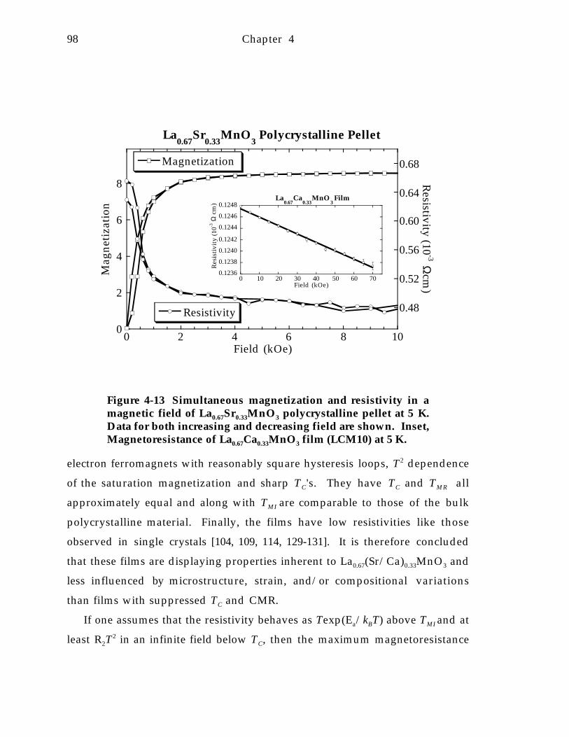
98 Chapter 4

electron ferromagnets with reasonably square hysteresis loops, T2 dependence

of the saturation magnetization and sharp TC's. They have TC and TMR all

approximately equal and along with TMI are comparable to those of the bulk

polycrystalline material. Finally, the films have low resistivities like those

observed in single crystals [104, 109, 114, 129-131]. It is therefore concluded

that these films are displaying properties inherent to La0.67(Sr/Ca)0.33MnO3 and

less influenced by microstructure, strain, and/or compositional variations

than films with suppressed TC and CMR.

If one assumes that the resistivity behaves as Texp(Ea/kBT) above TMI and at

least R2T2 in an infinite field below TC, then the maximum magnetoresistance

0

2

4

6

8

0.48

0.52

0.56

0.60

0.64

0.68

0 2 4 6 8 10

La0.67

Sr0.33

MnO3 Polycrystalline Pellet

Magnetization

Resistivity

Mag

neti

zati

on

Resistivity (10

-3 Ωcm

)

Field (kOe)

0.1236

0.1238

0.1240

0.1242

0.1244

0.1246

0.1248

0 10 20 30 40 50 60 70

La0.67

Ca0.33

MnO3 Film

Res

isti

vity

(10-3

Ω c

m)

Field (kOe)

Figure 4-13 Simultaneous magnetization and resistivity in amagnetic field of La0.67Sr0.33MnO3 polycrystalline pellet at 5 K.Data for both increasing and decreasing field are shown. Inset,Magnetoresistance of La0.67Ca0.33MnO3 film (LCM10) at 5 K.

Intrinsic Properties of La0.67Ca0.33MnO3 99

(∆R/R(H) at T = TMR = TMI) follows exp(Ea/kBTMI)/(TMI ). This predicts

"colossal" magneto resistance only at low temperatures, as a consequence of

the depressed TMI. Such a strong dependence of the magnetoresistance on a

film's particular TMI has been documented (Appendices A and B) from the

various values reported in the literature.

4.2.8 Domain Boundary MagnetoresistanceThe negative magnetoresistance associated with the domain orientation is

only observed in polycrystalline samples [28, 96]. If this is due to domain wall

scattering, then films and crystals with fewer domain boundaries would be

expected to show a much smaller effect. It has been concluded that spin-

polarized inter-grain tunneling is responsible for this effect [132].

4. 2. 9 Low temperature magnetoresistanceThe low temperature negative magnetoresistance linear in H is very small

in the films but somewhat larger in the polycrystalline samples (Figure 4-13,

and [28, 96]). This negative magnetoresistance may be due to the M2

dependence of the resistivity described in section 7.2.4 [129, 130] combined

with a small forced magnetization. Classic magnetoresistance of metals is

generally positive but is often negative in ferromagnets.

4.3 ConclusionWell annealed MOCVD thin films show properties of bulk

La0.67Ca0.33MnO3 and La0.67Sr0.33MnO3. The limiting low temperature

resistivity of 0.2 mΩcm, which gives a mean free path of roughly 20Å, is

independent of alkaline earth element and only slightly dependent on field

for single crystal material (bulk or film). The manganites show a significant

T2 dependence of the resistivity which is also independent of alkaline earth

element and magnetic field. The maximum in the magnetoresistance occurs

at the Curie temperature, which is not necessarily where dρ/dT changes sign,

but where dρ/dT is a maximum. A large magnetoresistance can occur well

100 Chapter 4

above room temperature, but the effect decreases significantly with

temperature.

Three regions of magnetoresistance are identified in these materials. The

largest effect is likely due to the suppression of magnetic critical scattering

near the Curie temperature. There is also a negative magnetoresistance

associated with the net magnetization of polycrystalline samples but not seen

in single crystal materials. Finally there is a small negative

magnetoresistance linear in field even at low temperatures.

The compounds La0.67Ca0.33MnO3 and La0.67Sr0.33MnO3 are metallic

ferromagnets with large saturation moments. The saturation magnetization

is found to decrease proportional to T2.

The high temperature resistivity of La0.67Ca0.33MnO3 clearly follows the law

predicted by small polaron hopping conductivity both in the thermally

activated regime and at higher temperatures where scattering becomes

important. There appears to be a structural transition at about 750K.

The resistivity of La0.67Sr0.33MnO3 above the Curie temperature shows a

crossover from a metallic to a hopping regime at higher temperatures.

In conclusion, the CMR effects in materials of the same compositions as

those studied here but with much lower transition temperatures, are not

intrinsic to the thermodynamically stable phase. Local inhomogeneities or

noncrystallinity in not fully annealed films may suppress the magnetic and

metal-insulator transitions. This presumably causes the observed

superparamagnetic type magnetism and conduction via percolation.

101

5. Local Structure, Transport and Rare Earth Magnetism in

the Ferrimagnetic Perovskite Gd0.67Ca0.33MnO3

In order to examine the nature of the metal-insulator transition in the

CMR manganites, the distorted perovskite Gd0.67Ca0.33MnO3 related to

La0.67Ca0.33MnO3 was studied. The composition x = 1/3 was chosen because

this doping concentration should maximize the double exchange effect as

seen in the lanthanum compounds [29]. Due to the small size of the Gd3+

ion, Gd0.67Ca0.33MnO3 should be in the region of the x = 1/3 phase diagram

where there is no transition to a metallic state, but to a ferromagnetic

insulating state around 50K [100]. The ferromagnetic nature of this low

temperature state has recently been questioned due to evidence of a spin glass

behavior with no long range ferromagnetic order in (TbxLa1-x)0.67Ca0.33MnO3

[136]. The x-ray-absorption fine-structure (XAFS) technique can detect small

variations of the average local environment about a particular atomic species,

making it ideal for studying subtle structural phase transitions associated with

any metal-insulator or ferromagnetic transitions. The Mn K-edge (6.54 keV)

and Gd LIII-edge (7.25 keV) are well enough separated that there is little

interference of the Mn and Gd XAFS.

In this study, it is found that the rare earth moments in Gd0.67Ca0.33MnO3

order antiparallel to the manganese giving rise to ferrimagnetism.

Furthermore, not only does this material remain insulating when it becomes

magnetically ordered, but no structural difference exists between the

ferrimagnetic and paramagnetic state. This is consistent with models that

require a structural change, as well as the ferromagnetic ordering of the

manganese atoms, to explain the metal-insulator transition and the large

magnetoresistance that accompanies it. Most of the work presented in this

chapter has been previously published [137].

102 Chapter 5

5.1 FerrimagnetismThe polycrystalline pellets, crystals and thin films all display a

ferromagnetic transition and a compensation temperature (Figure 5-1), which

is characteristic of ferrimagnets. Both bulk materials, polycrystalline pellet

and float zone crystal, have very similar magnetic properties while the film is

slightly different.

Gd0.67Ca0.33MnO3 displays the properties of a ferrimagnet, much like the

garnet ferrite Gd3Fe5O3 [138]. At about 60K, the transition metal spins order,

dominating the magnetization. As the temperature is lowered, the opposing

magnetization of the weaker coupled rare earth ions increases, since they

behave almost as though they were free paramagnetic spins reacting to an

internal field (section 5.1.3, Figure 3-19).

At the compensation temperature, TComp, the rare earth and transition

metal sublattice magnetizations exactly cancel (in zero field). Below TComp, the

magnetization of the rare earth ions, which have larger spins, dominates.

This is best seen in zero field remnant data which shows the magnetization

changing sign at TComp.

In the presence of magnetic fields greater than the coercive field, the

stronger sublattice flips to align parallel with the field, giving the minimum

in M at TComp as seen the 5 kOe data.

Local Structure and Magnetism in Gd0.67Ca0.33MnO3 103

-0.2

0.0

0.2

0.4

0.6

0.8

1.0

1.2

0 10 20 30 40 50 60 70 80 90

Gd0.67

Ca0.33

MnO3 Magnetization

Mag

neti

zati

on (

µ B/

mol

e)

Temperature (K)

5kOe

Remnant

CrystalPelletFilm

× 25

Figure 5-1 Low temperature magnetization ofGd0.67Ca0.33MnO3 measured in a 5 kOe field and zero field aftercooling in a large field (remnant).

5. 1. 1 Low temperature momentThe saturation magnetization per mole of Gd0.67Ca0.33MnO3 expected from

the Gd3+ S = 7/2, l = 0 is µ=(0.67 × 2 × 7/2) µB = 4.67µB, while high spin

manganese gives spin only (orbital contribution quenched) µ = gSµB, g = 2 so µ

= 2µB[0.67 × 2 (from Mn3+) + 0.33 × 3/2 (from Mn4+)] = 3.67µB. The simple two

sublattice (Gd and Mn) ferrimagnetism described above predicts a zero

temperature saturation magnetization of 4.67 µB - 3.67 µB = 1.00 µB (if there is

any canting of the sublattices such as that in Pr0.67Ca0.33MnO3 [139], a smaller

moment is predicted). This is roughly what is observed. The mean field

104 Chapter 5

calculation predicts a constant moment for T < 5 K, while the data show an

almost linear change in M for 2 K < T < 5 K. Also, the peak in the

magnetization, observed at about 50 K in the 5 kOe data is less than the 1.9µB

predicted in the mean field calculation.

5. 1. 2 High temperature susceptibilitySusceptibility data (Figure 5-2) above 200 K fit to the Curie-Weiss law:

χ = µeff2/(8(T-Θ)) with Θ = 34 K and µeff

2= 71 µB2. The difference in the

susceptibility of the crystal compared to that of the pellet at high temperatures

may not be significant. For quantum mechanical spins µeff2 per mole is

expected to be 63 µB2: 22µB

2(0.67 × 4/2 × 6/2) = 16 µB2 from Mn3+; 22µB

2(0.33 ×

3/2 × 5/2) = 5 µB2 from Mn4+; 22µB

2 (0.67 × 7/2 × 9/2) = 42 µB2 from Gd3+. This

extra moment, which is also observed in La0.67Ca0.33MnO3 [103] section 4.1,

may be due to the orbital contribution in the manganese ions. Since the two

sublattices have different coupling energies, the susceptibility above TC will

not obey a simple Curie-Weiss law even in the mean field approximation

(Figure 5-5). The simple mean field model of the above ferrimagnetism

requires TC/Θ > 3, as described in section 3.2.2.4.1. This is clearly not the case

for the measured parameters. Alternatively, the addition of a Pauli-like

susceptibility χ0 to the fit, χ = χ0 + µeff2/(8(T-Θ)), will reduce the contribution

from µeff. For example, an equally good fit to the data can be found with

µeff2 = 63 µB

2, χ0 = 7.7 × 10-6 emu G-1 g-1, and Θ = 50 K.

Local Structure and Magnetism in Gd0.67Ca0.33MnO3 105

0

5

10

15

20

25

30

35

40

0 50 100 150 200 250 300 350 400

Gd0.67

Ca0.33

MnO3 Susceptibility

1/χ m

ol (

Gau

ss·m

ol/

emu

)

Temperature (K)

5 kOeCrystalPellet

Figure 5-2 Inverse magnetic susceptibility of bulkGd0.67Ca0.33MnO3. Solid line is the high temperature fit to χ =µeff

2/(8(T-Θ)) described in the text.

5. 1. 3 Low temperature susceptibilityBetween TComp and TC, the magnetic susceptibility essentially that of the

paramagnetic-like rare earth moments, showing an approximate

χ ∝ 1/(T + TComp). Below TComp the Gd3+ moments effectively order antiferro-

magnetically with respect to the manganese moments, and so the

susceptibility decreases below TComp.

106 Chapter 5

0.20

0.24

0.28

0.32

0.36

0.40

0 10 20 30 40 50 60 70 80

High Field Susceptibility of Gd0.67

Ca0.33

MnO3

χ mol

( µB/

mol

/T

)

Temperature (K)

0

1

2

3

0 10 20 30 40 50 60 70Mag

neti

zati

on ( µ

B/

mol

e)

Magnetic Field (kOe)

5K

Figure 5-3 Low temperature and high-field magneticsusceptibility, χ = (M(60 kOe)-M(40 kOe))/20kOe, ofGd0.67Ca0.33MnO3 crystal. Inset, hysteresis loop at 5 K.

The hysteresis loop at 5 K (Figure 5-3) shows an additional high field

paramagnetic response not expected for a mean field ferrimagnet. It is not

uncommon, however, to observe such a field-induced increase of the

magnetization in canted ferromagnetic or ferrimagnetic systems [140, 141],

and is used as evidence of the ferrimagnetic sublattices canting away from

antiparallel [101]. The magnetic field affects the canting angle, which results

in the magnetization increasing nearly linearly with field even at T = 0 K

[140]. If this large susceptibility were due to a second phase with free

paramagnetic spins, then this phase would have to contain at least half of the

available spins and have a 1/T temperature dependence for all T. This is not

Local Structure and Magnetism in Gd0.67Ca0.33MnO3 107

seen in Figure 5-3. Instead, the high field susceptibility maximizes near TComp

which is typical of an antiferromagnet with TN ≈ TComp. This is predicted in the

mean field calculation for a ferrimagnet described in section 3.2.2.4.1.

5. 1. 4 Near TC magnetismThe experimental values of TC are summarized in Table 5-1. An example

0.00

0.02

0.04

0.06

0.08

0.10

0 2000 4000 6000 8000 10000

Gd0.67

Ca0.33

MnO3 Arrott Plot

35K40K45K50K55K60K70K

Mag

neti

zati

on2 (µ

B/

mol

e)2

H/M (Oe/µB)

Figure 5-4 Arrott plot of polycrystalline Gd0.67Ca0.33MnO3

pellet.

Table 5-1 Transition Temperatures for Gd0.67Ca0.33MnO3.

TComp Arrott TC Remnant TC Inflection TC

Polycrystalline Pellet 17K 52K 60K 80KSingle Crystal 17K 56K 62K 78KThin Film 13K 70K 81K 88K

108 Chapter 5

of the nonlinear M2 vs. H/M Arrott plot is given in Figure 5-4.

5. 1. 5 Magnetism modelTo explain the magnetism, a mean field model was used assuming a

ferrimagnetic ground state. Other possible explanations for the magnetism i n

Gd0.67Ca0.33MnO3 are briefly discussed

0 50 100 150 200 250 300

Gd0.67

Ca0.33

MnO3 Mean Field Calculation

0

5

10

15

20

25

30

35

40

1/χ (m

ol G/

emu)

Temperature (K)

5 kOe

20 40 60 80 100-5-4

-3-2-1

0123 M

agnetization (µB /

mol)

Temperature (K)

Gd

Mn

5 kOe

Remnant

Figure 5-5 Magnetization and inverse magnetic susceptibilitycalculated for Gd0.67Ca0.33MnO3 using the simplified mean fieldtheory described in the text and TC = 83 K, TComp = 17 K. Thecontribution to the magnetization of each sublattice is shownin dashed lines.

5. 1. 5. 1 Mean Field ModelDue to the stronger 3d exchange interaction compared to that of the 4f, the

Mn-Mn coupling is expected to be stronger than the Mn-Gd, and the Gd-Gd

interaction to be negligible. Since the observed Curie temperature is about

Local Structure and Magnetism in Gd0.67Ca0.33MnO3 109

that expected from the trend found in the manganese ferromagnetic ordering

temperature as a function of the average of the R and A atom sizes i n

R1-xAxMnO3 [100], it is assumed for now that the Mn-Mn interaction i n

Gd0.67Ca0.33MnO3 is ferromagnetic. The ferrimagnetism must then arise from

a weaker, antiferromagnetic Mn-Gd interaction. Thus, unlike the ferrites,

where the dominant interaction is antiferromagnetic between the two

transition metal sublattices, the strongest magnetic coupling i n

Gd0.67Ca0.33MnO3 is ferromagnetic, much like that found in the rare earth

cobaltites, e. g. GdCo5 [142].

The above description of the magnetization can be bolstered using a

simple molecular or mean field model described in section 3.2.2.4. Assuming

that all atoms on each sublattice (Mn or Gd) feel the same mean field, there

are only two unknown mean field coefficients due to the Mn-Mn and Mn-Gd

interactions. These two coefficients are easily determined since they are

nearly proportional to TC and TComp, respectively. This molecular field model

(Figure 5-5) reproduces the qualitative features described above.

The calculated magnetization and inverse susceptibility for the molecular

field model described below is shown in Figure 5-5.

This model is limited by the obvious simplifications: not only are there

two distinct types of Mn atoms (Mn3+ and Mn4+), but there are numerous

possible configurations for the number and type of near neighbors due to the

randomness on the Mn and Gd/Ca sites. The discrepancy among the various

values of TC determined by the three methods mentioned is an example of

non-mean-field ferromagnetic behavior. The discrepancies in the salient

features discussed above may result from the simplifications of the model,

and the assumptions behind it.

5. 1. 5. 2 Canted antiferromagnetismThe evidence concerning the magnetic structure of the manganese in the

ferromagnetic insulator phase points to a canted antiferromagnetic structure

110 Chapter 5

rather than a simple ferromagnet. The magnetic structure of Pr0.67Ca0.33MnO3

which is on the boundary between ferromagnetic-insulator and ferro-

magnetic-metal low temperature phases [100], has been extensively studied.

Neutron diffraction shows Pr0.67Ca0.33MnO3 to have a charge-ordered, canted-

antiferromagnetic structure in the low temperature phase with ferromagnetic

moment about half of the total expected moment [139, 143]. A compound

clearly in the ferromagnetic-insulator part of the tolerance-factor phase-

diagram (Figure 3-17), much closer to Gd0.67Ca0.33MnO3 than Pr0.67Ca0.33MnO3

is La0.2Y0.5Ca0.3MnO3. This compound appears to be ferromagnetic with about

half the expected ferromagnetic moment [100], which could be explained by a

canted antiferromagnetic state similar to that found in Pr0.67Ca0.33MnO3. Thus,

one should expect the ferromagnetic moment of the Mn ions i n

Gd0.67Ca0.33MnO3 to be half that predicted in the above molecular field model.

If the Gd moments are also canted to the same degree, then the predicted

magnetization will be qualitatively the same for the uncanted case

(Figure 5-5), only half the magnitude; namely, there will still be a

compensation temperature.

5. 1. 5. 3 Spin glass magnetismAtomic disorder such as that found on both the Gd and Mn site i n

Gd0.67Ca0.33MnO3 can result in a spin-glass, and indeed a spin-glass insulating

low-temperature phase was found in (TbxLa1-x)0.67Ca0.33MnO3 in place of the

ferromagnetic insulator state. The compound Tb0.67Ca0.33MnO3 should be i n

the same region of the tolerance-factor phase-diagram as Gd0.67Ca0.33MnO3 and

La0.2Y0.5Ca0.3MnO3. The Tb compound is apparently a pure spin-glass with no

long-range magnetic order [136]. A full investigation of the existence or non-

existence of spin-glass behavior in Gd0.67Ca0.33MnO3 is beyond the scope of this

work. However, it is clear that Gd0.67Ca0.33MnO3 has long range magnetic

order, which eliminates the possibility of a spin glass. The distinction is most

obvious in the Arrott plot (Figure 4), which shows that Gd0.67Ca0.33MnO3 has a

Local Structure and Magnetism in Gd0.67Ca0.33MnO3 111

non-zero magnetization when H = 0 below TC, while

(Tb0.33La0.67)0.67Ca0.33MnO3 does not [136]. The other striking feature of

Gd0.67Ca0.33MnO3 is the existence of a compensation point, which to our

knowledge cannot be explained by a spin-glass magnetic system.

5. 1. 5. 4 Related CompoundsSince Gd3+ has the largest spin of the rare earth elements, it should have

the highest ordering temperature. If the relevant exchange interaction is due

to spin-spin coupling of the rare earth and manganese atoms, then the

strength of this interaction will be proportional to the spin S of the rare earth

-6

-4

-2

0

2

4

6

1 2 3 4 5 6 7

Gd0.67

Ca0.33

MnO3 High Temp. Resistivity

ln( ρ

/T

(Ω c

m/

K))

1000/T (1000/K)

a

b

1

2

3

4

0.18 0.20 0.22ln

( ρ/

Ω c

m)

1/T1/4 (K-1/4)

1

2

3

4

1.0 1.5 2.0 2.5 3.0

ln( ρ

/Ω

cm

)

1000/T (1000/K)

Figure 5-6 High temperature resistivity during heating andcooling a Gd0.67Ca0.33MnO3 film, ln(ρ/T) vs. 1/T . Inset a,comparison with ln(ρ) vs. 1/T. Inset b, comparison with ln(ρ)vs. 1/T 1/4.

112 Chapter 5

ion. From this relation the ordering temperature of the rare earth moments

in related compounds is estimated to be about 7 K for Nd0.67Ca0.33MnO3 and

5 K for Pr0.67Ca0.33MnO3. This should result in a decrease in M at low T. This

appears at temperatures lower than these estimates, if at all [23, 144]; perhaps

indicating an interaction strength proportional to S2, the square of the rare

earth spin, or simply that these moments do not order antiparallel to the

manganese moments [145].

10

12

14

16

18

20

22

24

0.32 0.33 0.34 0.35 0.36 0.37 0.38

Gd0.67

Ca0.33

MnO3 Low Temperature Resistivity

ln( ρ

/Ω

cm

)

1/T1/4 (K-1/4)

65 K ≈ Tc

a

b

-0.8

-0.6

-0.4

-0.2

0.0

-3

-2

-1

0

-60 -40 -20 0 20 40 6030

0K M

R (%

) 200K M

R (%

)

Field (kOe)

300K200K

5

10

15

20

10 12 14 16 18 20 22

ln( ρ

/T

(Ω c

m/

K))

1000/T (1/K)

Figure 5-7 Low temperature resistivity of Gd0.67Ca0.33MnO3

crystal, ln(ρ) vs. 1/T 1/4. Inset a, comparison with ln(ρ/T) vs.1/T. Solid lines show linear best fit to the data shown. Inset b,magnetoresistance of a film at 200 K and 300 K; solid line isthe quadratic fit.

Local Structure and Magnetism in Gd0.67Ca0.33MnO3 113

5.2 Electronic TransportThe resistivity can be well approximated by RhTexp(Ea/kBT) (Figure 5-6),

predicted by small polaron hopping conductivity [68, 146]. Below about 150 K

(Figure 5-7), the resistivity is somewhat better described by R0exp(T0/T)1/4,

which is commonly attributed to variable range hopping [123]. The

quantitative aspects of the fits is discussed below. The thin film and crystal

samples show no transition to a metallic state down to 5 K.

5. 2. 1 MagnetoresistanceNo extraordinary magnetoresistance was observed in the entire

temperature range. The magnetoresistance at 200 K and 300 K is a few percent

in a 70 kOe field and approximately proportional to H2 (Figure 5-7). Reliable

resistivity data could be measured on the crystal sample down to 40 K. No

discontinuity in the resistivity was found near TC.

5. 2. 2 Small Polaron HoppingThe electrical resistivity of Gd0.67Ca0.33MnO3 is consistent with adiabatic

small polaron hopping conductivity (section 4.2.6)RhTexp(Ea/kBT) [58, 68]

Rh = 2kB/3ne2a2ν particularly at high temperatures. Here, kB is Boltzmann’s

constant, e is the electronic charge, n is the number density of charge carriers

— about 0.7 carrier per Mn, a is the site-to-site hopping distance, and ν is the

longitudinal optical phonon frequency. This behavior has also been observed

in the La containing compound described in section 4.2.2 [103, 146].

Resistivity data are often displayed on an Arrhenius plot (ln(ρ) vs. 1/T) which

will give a straight line for a band gap semiconductor [15, 147]. The slightly

different temperature dependence of the data provides the significant

nonlinearity in such a fit (Figure 5-6). A polaron hopping activation energy,

Ea, of 1940K, and an attempt frequency of 8 × 1013 s-1 is inferred. The small

polaron mechanism implies that unlike a bandgap semiconductor, the highly

temperature dependent quantity is the mobility, not the carrier concentration.

114 Chapter 5

A high, temperature independent carrier concentration is consistent with

Hall effect measurements (sect 4.2.4) on La0.67Ca0.33MnO3.

5. 2. 3 Variable Range HoppingThe resistivity of the manganites has also been attributed to variable range

hopping due to Anderson localization [148]. At temperatures less than 150K,

this picture produces a somewhat better fit to our data (Figure 5-7), but is

clearly inferior to the polaron model at high temperatures (Figure 5-6). The

fit to R0exp(T0/T)1/4 gives T0 = 1.7 × 109 K. In the theory of variable range

hopping [71, 149], kB T0 ≈ 21/(ζ3N(EF)) where ζ is the decay length of the

localized wave function, and N(EF) is the density of localized states at the

Fermi level. For ζ ≈ a = 3.9Å, the distance between neighboring Mn atoms,

this implies N(EF) ≈ 2.4 × 1018 eV-1 cm-3 which is typical for disorder

semiconductors but about 1500 times less than the density of states found i n

the specific heat of manganites which become metallic at low temperatures

(≈ 5 mJ mol-1 K-2)[124].

5.3 X-ray Absorption Fine Structure

The primary quantity in XAFS data analyses is χ(k)=(µ(k)-µ0(k))/µ0(k)),

where k is the ejected photoelectron wave vector, µ(k) is the total absorption

due to the absorbing atomic species, and µ0(k)) is the portion of µ(k) that does

not include the photoelectron backscattering off neighboring atoms. This

backscattering causes an interference at the absorbing atom which is manifest

as oscillations in χ(k). A Fourier transform of kχ(k) thus produces peaks that

correspond to the distribution of atoms around the absorbing atom.

Figure 5-8 shows these Fourier transforms.

Local Structure and Magnetism in Gd0.67Ca0.33MnO3 115

Figure 5-8 Fourier transform of kχ(k) from (a) Mn K-edge and(b) Gd LIII-edge data on Gd0.67Ca0.33MnO3 . The solid lines aredata collected at T = 69 K, while the triangles (∆) are datacollected at T = 40 K. Agreement between data above andbelow TC is well within the errors of the experiment.Transform ranges for the Gd edge data are from 3.5-12.5 Å-1

and Gaussian broadened by 0.3 Å-1. Transform ranges for theMn edge data are from 3.2-12.5 Å-1 and Gaussian broadened by0.3 Å-1.

The agreement between the data above and below TC is very good and

places limits on any atom-position changes around either the Gd or M n

atoms within ±0.005 Å, and changes in the Debye-Waller broadening factor to

±0.002 Å (Pnma; a = 5.52Å, b = 7.50Å, c = 5.34Å).

116 Chapter 5

5. 3. 1 Relationship of structure to CMRUnlike the colossal magnetoresistance manganites, Gd0.67Ca0.33MnO3 does

not have a metal-insulator transition or a large magnetoresistance near the

Curie temperature. The negative magnetoresistance is only of order 1% i n

large fields and is proportional to H2 (or M2 since it scales with χ2) like that

observed in La0.67Ca0.33MnO3 in the paramagnetic state (section 7.2.1) [150].

Thus, Gd0.67Ca0.33MnO3 is clearly in the class of 1/3 doped manganites which,

due to the small size of Gd3+ [100], change from paramagnetic insulators to

ferromagnetic insulators at TC. There is much interest in finding a structural

change at TC in the giant magnetoresistive manganites, since it is predicted to

have a large effect on the resistive transition [11]. There is now evidence [151-

154] for a decrease in structural disorder as the GMR manganites become

ferromagnetic metals. Gd0.67Ca0.33MnO3 shows the contrapositive: there is no

discontinuity in the atomic disorder for a material which does not become

metallic at TC. This has also been noted in manganites with different dopant

concentrations: La0.88Ca0.12MnO3 [151] and La0.5Ca0.5MnO3 [154].

5.4 ConclusionGd0.67Ca0.33MnO3 is ferrimagnetic with a compensation temperature of

about 15K due to the interaction and ordering of the Gd3+ ions. The

qualitative features of the magnetic properties can be accounted for with a

simple two sublattice (Gd and Mn) molecular field model. The large high

field susceptibility at low temperatures may indicate a canting of the magnetic

sublattices. Contrary to the conclusion in [136] that there does not exist long-

range magnetic order (only spin-glass magnetism) in the ferromagnetic-

insulator region of the tolerance-factor phase-diagram, Gd0.67Ca0.33MnO3

shows definite long-range order and a compensation point which can not be

explained by spin-glass phenomena alone. The resistivity is consistent with

small polaron conductivity over a broad temperature range, with a possible

crossover to a different mechanism such as variable-range hopping at low

Local Structure and Magnetism in Gd0.67Ca0.33MnO3 117

temperatures. There is no noticeable change in the structure, as determined

by XAFS, or conductivity at the ferrimagnetic transition. Recent theoretical

and experimental work conclude that structural effects at TC are associated

with the metal-insulator transition and large magnetoresistance. Since

Gd0.67Ca0.33MnO3 is in the doping regime where a metal-insulator transition

and large magnetoresistance are not observed at TC, this work supports that

conclusion, i. e. that a significant structural change is associated not with the

ferromagnetic transition, but the metal-insulator transition.

118

6. Magnetoconductivity in La0.67Ca0.33MnO3

In this chapter, the nature of the field dependence of the resistivity i n

La0.67Ca0.33MnO3 - or magnetoresistance above and below TC is studied in more

detail. For this study, sample LCM 17 (Chapter 4, Table 4-2) was used since it

shows magnetic and transport properties consistent with bulk samples.

Measurements at 0.9TC = 237 K and 1.1TC = 289 K will have considerable

magnetoresistance while being clearly either in the ferromagnetic or

paramagnetic state. In order to achieve maximum temperature stability, data

were collected only after there was no appreciable drift in the resistivity. The

major conclusions have been reproduced with other samples which like this

one have high TC’s and no domain boundary magnetoresistance (section

4.2.8). The work presented in this chapter has been published in [150].

Two configurations were used: 1) magnetic field parallel to the film,

which was used for longitudinal and transverse magnetoresistance analysis

since there is almost no demagnetization field. Since the van der Pauw

configuration is used, the longitudinal magnetoresistance has a small

component due to transverse magnetoresistance and vice versa. 2) magnetic

field perpendicular to the film, used primarily for Hall effect measurements.

6.1 Anisotropic magnetoresistanceThe magnetoresistance at 289 K (1.1TC) on increasing and decreasing

magnetic field is displayed in Figure 6-1 for longitudinal and transverse

directions. The two configurations give identical magnetoresistance.

The high field (|H| > 1 kOe) magnetoresistance at 0.9TC is also shown i n

Figure 6-1 for both increasing and decreasing fields. There is no appreciable

hysteresis for |H| > 200 Oe. The transverse and longitudinal

magnetoresistance in high fields are nearly identical when the same current

path is used. Different current paths however, give a slightly different

Magnetoconductivity in La0.67Ca0.33MnO3 119

magnetoresistance at 0.9TC indicating some magnetic/electronic

inhomogeneity below TC. All current paths have the functional form of the

magnetoresistance described below, and therefore the apparent

inhomogeneity does not affect the conclusions of this paper. The transverse

magnetoresistance with the field perpendicular to the film is identical to the

transverse magnetoresistance with the field parallel to the film with an

additional demagnetization field of (1750+/-100 Oe); this was used to estimate

M at 0.9 TC.

6.2 Magnetoresistance modelsIn order to assess the potential of the colossal magnetoresistance in a

magnetic field sensor, (such as the read head in a magnetic recording device)

knowledge of the magnitude and exact field dependence of the

magnetoresistance is critical, primarily in low magnetic fields, H.

Experimental data generally show that for low fields the magnetoresistance is

approximately quadratic in H above the Curie temperature, TC and is more

cusp like or linear below TC [116]. There exists, however, many counter

examples to this generalization [22, 25, 114] presumably due to inhomogenous

samples where TC is not so well defined [116]. The best empirical model of the

resistivity (ρ = ρ0eM/M

0) around TC [114] gives a linear field dependence. Since

the earliest reports [4], the magnetoresistance has been claimed or assumed to

be independent of the angle between the magnetic field and the current [113].

The microscopic mechanism of the magnetoresistance can be quite

complicated and still not accurately predict much of the observed

magnetoresistance phenomena. Much of the theory assumes an electron

band transport mechanism [55], which may not be appropriate in the case of

the manganites because they are not metallic above TC. Some microscopic

models of transport in the manganites have predicted the conductivity σ or

120 Chapter 6

resistivity ρ ∝ M2 [113, 155, 156] (which is isotropic) with limited experimental

verification.

6. 2. 1 General ModelThe difference above and below TC as well as the relationship to the

magnetization M can be shown more generally by only considering the

symmetry of the resistivity tensor - with no assumptions about or even a

reference to microscopic transport mechanisms. Following Landau and

Lifshitz [157], the relation between the electric field E and the current density J

is given by the resistivity tensor ρ: Ei = ρikJk where the components of ρ are

functions of H and M. Since H and M are vectors which are antisymmetric

under time reversal, ρ must have the following symmetry: ρik(H,M) =

ρki(-H,M) = ρki(H,-M) = ρik(-H,-M). The symmetric, sik, and antisymmetric, aik,

parts of ρik = sik + aik then have the following properties: sik(H,M) = sik(-H,M) =

sik(H,-M) and aik(H,M) = -aik(-H,M) = -aik(H,-M). Thus the components of sik are

even functions of H and M while those of aik are odd functions.

The measured resistivity ρ, the diagonal component of the resistivity

tensor, contains no contribution from aik and therefore must be even in H and

M. Assuming the resistivity is an analytic function with respect to H and M

(which themselves may not be analytic in T), the first terms in the expansion

of ρ in powers of H and M is then ρ = ρ0 + αM2 + βH2 + γH•M. At this point,

one can already expect that for T > TC (M=0) the low field magnetoresistance

should be proportional to H2 while for T < TC (M≠0) the term linear in H may

be expected to dominate. Clearly a negative magnetoresistance can not obey

this relation for arbitrarily large H, for the resistivity would eventually

become negative; higher order terms or inverse powers of H are then

required. The above argument is as valid for the conductivity tensor σ, where

Ji = σikEk, as it is for ρ. In the case of the manganites, the magnetoconductivity

Magnetoconductivity in La0.67Ca0.33MnO3 121

is positive and unlike the magnetoresistance may not require further

expansion in H.

6. 2. 1. 1 Magnetoconductivity modelFor an isotropic conductor the longitudinal and transverse

magnetoconductances (and magnetoresistances) are, in general, not equal.

The general form of the relation between J and E in an isotropic conductor

[157] up to terms quadratic in H and M is:

J = σ0E + α1M2E + α2(E•M)M +

β1H2E + β2(E•H)H +

γ1(H•M)E + γ2(M•E)H + γ3(E•H)M + (1)

σHH×E + σAM×E

If all the coefficients (except α1) are allowed to be functions of M2, (e.g.

σ0 → σ0 + α 1M2 + … ) then (1) is a complete expansion in H up to H2 and all

powers of M.

The βi terms provide the M = 0 magnetoconductance quadratic in H.

When β2 = 0, the longitudinal and transverse magnetoconductances are

equal. Similarly, the α2 term leads to magnetoconductance depending on the

angle between E and M - known as anisotropic magnetoresistance 6.1. The γi

provide magnetoconductance linear in H only when M ≠ 0. The equation

used to fit the data is formally equivalent to a circuit containing a resistor (ρ∞)

in series with the magnetoconductor (e.g. σ(H) = σ0 + σΗ2H2), although the

physical significance of such an equivalent circuit is not entirely clear. In any

event, ρ∞ is presumably the intrinsic spin independent resistivity found to be

proportional to a constant plus a T2 term, described in sections 4.2.1 and 7.2.2

[103].

122 Chapter 6

The Hall effects are contained in the antisymmetric part of σ and ρ and

therefore can be expanded in odd powers of H and M. The first two terms i n

the Hall resistivity is RHH×J + RAM×J, where RH is the normal Hall coefficient

and RA is the anomalous Hall coefficient. Since there is no evidence to prefer

the Hall conductivity of equation 1 (≈ -RH/H2) to the Hall resistivity, the Hall

effect is analyzed using RH and RA.

It is possible that the observed magnetoconductivity could be reduced to

terms involving only M2 and (E•M)M since M ≈ M0 + χH gives the same field

dependence described above. This would imply a strict relationship among

the various βi(T) and γi(T) which could be determined by simultaneous

measurements of M and the magnetoconductivity. The resistivity saturates

in a magnetic field [113, 158] more rapidly than does the magnetization

(giving M2 behavior only at small M), indicating again that it is probably the

conductivity not the resistivity which is proportional to M2. This is discussed

in more detail in chapter 7.

The reciprocal nature of the conductivity and resistivity leads to only an

abstract distinction between them. Thus, the simpler, empirical description of

the resistivity in terms of a magnetoconductivity may be accidental.

Nevertheless, it warrants further consideration. The standard additive

scattering time interpretation of the magnetoresistivity requires a more

complex H dependence to describe the suppression of magnetic scattering by a

magnetic field. The simplicity of the magnetoconductivity expression may

signify the basis of an alternative transport interpretation. Taken literally, the

magnetic field appears to open parallel channels of conduction with a simple,

physical functional dependence.

Magnetoconductivity in La0.67Ca0.33MnO3 123

6.2.1.1.1 T > TC regime

The 1.1TC data fit very well with three parameters (ρ∞ = 1.3 mΩcm, σο =

0.14 (mΩcm)-1 and σΗ2 = 43 × 10-6 (mΩcm)-1 (kOe)-2) to ρ(H) = ρ∞ + 1/(σ0 + βH2).

A much less satisfactory fit is obtained with ρ(H) = ρ(0) + aH2 + bH4.

Above TC, M = 0 (or at least M = χH which gives the same field

dependence of σ) so the diagonal element of the isotropic magneto-

conductance tensor σ(H) = σ0 + β1H2 + β2(E•H)2/E2. From the fit described

above at 1.1 TC, β1 = 43 × 10-6 (mΩcm)-1 (kOe)-2 and β2 ≈ 0 is estimated.

-60

-50

-40

-30

-20

-10

0

10

-80 -60 -40 -20 0 20 40 60 80

La0.67

Ca0.33

MnO3

Mag

neto

Res

ista

nce

∆R/R

(0) (

%)

Magnetic Field (kOe)

T = 1.1Tc

T = 0.9Tc

ρ∞

1/σ0

1/βH 2 or 1/γ|Η|

Figure 6-1 High field (longitudinal) magnetoresistance aboveand below TC for La0.67Ca0.33MnO3 film. The solid lines showthe fit using the indicated equivalent circuit

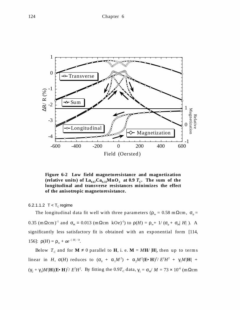
124 Chapter 6

-4

-3

-2

-1

0

1

-600 -400 -200 0 200 400 600-1

0

1

2

3

4

∆R/

R (%

)

Field (Oersted)

Transverse

Sum

Longitudinal

Relative

MagnetizationMagnetization

Figure 6-2 Low field magnetoresistance and magnetization(relative units) of La0.67Ca0.33MnO3 at 0.9 TC. The sum of thelongitudinal and transverse resistances minimizes the effectof the anisotropic magnetoresistance.

6.2.1.1.2 T < TC regime

The longitudinal data fit well with three parameters (ρ∞ = 0.58 mΩcm, σο =

0.35 (mΩcm)-1 and σΗ = 0.013 (mΩcm kOe)-1) to ρ(H) = ρ∞+ 1/(σο + σΗ|H|). A

significantly less satisfactory fit is obtained with an exponential form [114,

156]: ρ(H) = ρ∞ + ae -|H|/b.

Below TC and for M ≠ 0 parallel to H, i. e. M = MH/|H|, then up to terms

linear in H, σ(H) reduces to (σ0 + α 1M2) + α2M

2(E•H)2/E2H2 + γ1M|H| +

(γ2 + γ3)M|H|(E•H)2/E2H2. By fitting the 0.9TC data, γ1 = σΗ/M = 73 × 10-6 (mΩcm

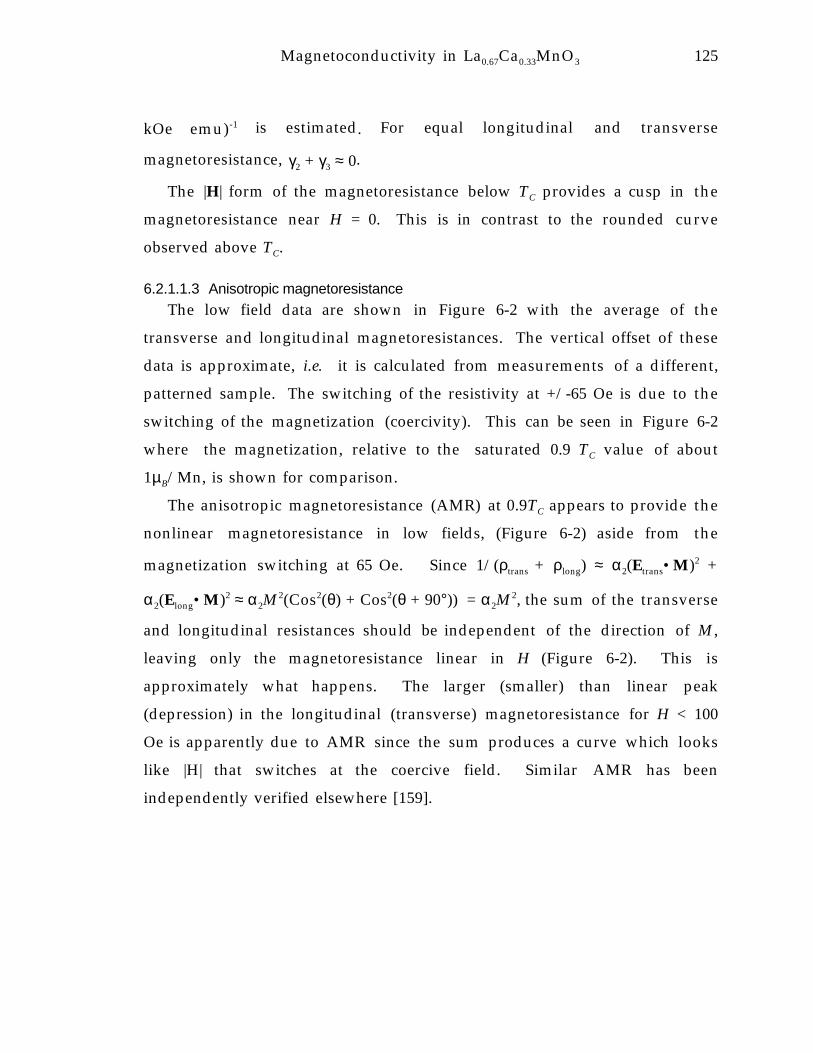
Magnetoconductivity in La0.67Ca0.33MnO3 125

kOe emu)-1 is estimated. For equal longitudinal and transverse

magnetoresistance, γ2 + γ3 ≈ 0.

The |H| form of the magnetoresistance below TC provides a cusp in the

magnetoresistance near H = 0. This is in contrast to the rounded curve

observed above TC.

6.2.1.1.3 Anisotropic magnetoresistance

The low field data are shown in Figure 6-2 with the average of the

transverse and longitudinal magnetoresistances. The vertical offset of these

data is approximate, i.e. it is calculated from measurements of a different,

patterned sample. The switching of the resistivity at +/-65 Oe is due to the

switching of the magnetization (coercivity). This can be seen in Figure 6-2

where the magnetization, relative to the saturated 0.9 TC value of about

1µB/Mn, is shown for comparison.

The anisotropic magnetoresistance (AMR) at 0.9TC appears to provide the

nonlinear magnetoresistance in low fields, (Figure 6-2) aside from the

magnetization switching at 65 Oe. Since 1/(ρtrans + ρlong) ≈ α2(Etrans•M)2 +

α2(Elong•M)2 ≈ α2M2(Cos2(θ) + Cos2(θ + 90°)) = α2M

2, the sum of the transverse

and longitudinal resistances should be independent of the direction of M,

leaving only the magnetoresistance linear in H (Figure 6-2). This is

approximately what happens. The larger (smaller) than linear peak

(depression) in the longitudinal (transverse) magnetoresistance for H < 100

Oe is apparently due to AMR since the sum produces a curve which looks

like |H| that switches at the coercive field. Similar AMR has been

independently verified elsewhere [159].

126 Chapter 6

6.2.1.1.4 Hall Effect

The Hall effect (Figure 6-3) is calculated from R(H) - R(-H), which should

remove all contributions to the transverse voltage due to magnetoresistance

and changes in magnetic homogeneity. The Hall effect at 0.9TC shows a clear

contribution at H=0 due to the anomalous Hall effect [160] as well as a term

linear in H. From this linear term, a carrier density of n = 0.85 holes/cell is

calculated which is the same as that observed at 5 K (section 4.2.4), where no

anomalous Hall effect was detected. The anomalous Hall effect apparently

increases with temperature, which is quite unexpected since it is usually

proportional to M [160]. Nevertheless, this has also been observed in the

magnetic spinels such as CuCr2Se4 [132-134]. At 1.1 TC the Hall effect has an

0.0

0.2

0.4

0.6

0.8

1.0

1.2

1.4

0 10 20 30 40 50 60 70

La0.67

Ca0.33

MnO3 Hall Effect

R(H

)-R

(-H

) (µ

Ω c

m)

Magnetic Field (kOe)

T = 1.1 TC

T = 0.9 TC

Figure 6-3 Hall effect of La0.67Ca0.33MnO3 below (fullymagnetized data only) and above TC.

Magnetoconductivity in La0.67Ca0.33MnO3 127

electron-like slope at low fields that slowly reverses to hole-like in high fields.

The low field slope can be attributed to the anomalous Hall effect resulting

from the magnetization due to the Curie-Weiss susceptibility, χ: Rhall = RAM +

RHH = (χRA + RH)H. Thus while the sample magnetizes the Hall effect looks

electron-like, but once the magnetization saturates, the Hall effect returns to

hole-like.

6.3 ConclusionIn summary, an accurate and simple model, based solely on symmetry

without reference to any mechanism, is proposed for the magnetoresistance

in La0.67Ca0.33MnO3. One can also conclude from this model that the

mechanism of the magnetotransport is best described by a

magnetoconductance, and therefore mechanistic theories should predict at

least a M2 dependence of the conductivity. The functional form and estimate

of parameters presented above should not only help guide the development

of a mechanistic theory, but also provide a basis for predicting the

magnetotransport properties when designing a device.

In homogeneous materials, it is clear that the magnetoresistance

maximizes near the ferromagnetic Curie temperature TC and rapidly

decreases at lower or higher temperatures. The magnetoresistance also slowly

saturates as the magnetic field is increased past several Tesla. Thus, the

conductivity behaves much like the magnetization: above TC the

conductivity and magnetization are low, while below TC the conductivity and

magnetization rapidly increase. Furthermore, near TC both the conductivity

and resistivity can be increased by an applied magnetic field. The theory of

double exchange, which has been developed to explain these properties of the

manganites [7, 112, 155], predicts this correlation between the conductivity and

the magnetization.

128

7. Critical Transport and Magnetization of La0.67Ca0.33MnO3

In homogeneous La0.67Ca0.33MnO3, it is clear that the magnetoresistance

maximizes near the ferromagnetic Curie temperature TC and rapidly

decreases at lower or higher temperatures. The magnetoresistance also slowly

saturates as the magnetic field is increased past several Tesla. Thus, the

conductivity behaves much like the magnetization: above TC the

conductivity and magnetization are low, while below TC the conductivity and

magnetization rapidly increase. Furthermore, near TC both the conductivity

and magnetic moment can be increased by an applied magnetic field. The

theory of double exchange, which has been developed to explain these

properties of the manganites [7, 112, 155], predicts this correlation between the

conductivity and the magnetization.

The relationship between the conductivity (or resistivity) and the

magnetization has been examined both experimentally and theoretically.

Several theoretical models [31, 112, 121, 155, 156, 161-164] predict an M2

dependence of the resistivity (or conductivity). The first term of the Taylor

series expansion of the resistivity (or conductivity) in terms of M should be

M2 for all models due to symmetry considerations [150].

Experimentally, a correlation between the resistivity and magnetization

can be found by plotting one as a function of the other [24, 114, 115, 121, 158,

165]. These plots show that the resistivity is roughly proportional to the

square of the magnetization M2 for small M. For larger M however, the

resistance decreases more slowly in relationship to M2 as if it were saturating

before the magnetization does. Thus the relationship between the resistivity

and the magnetization is more complicated than ρ ∝ M2. This relationship

may instead be well described by an M2 dependence of the conductivity in a

slightly more complicated circuit [150]. In the previous chapter, only the

Critical Transport and Magnetization of La0.67Ca0.33MnO3 129

magnetic field H dependence of the resistivity is shown to be more fully

described in terms of a magnetoconductive circuit, ρ = ρ∞ + 1/(σ0 + σH2H2) for

T > TC and ρ = ρ∞ + 1/(σ0 + σH|H|) for T < TC, where ρ∞, σ0, σH2 and σH are

parameters. In order to determine if the magnetoconductivity, σH2H2 and

σH|H| can replaced by a common term proportional to M2 as suggested above,

the temperature dependencies and magnitudes of σH2, σH and M need to be

examined.

Alternatively, it has been found in several cases that the correlation

ρ ∝ exp[-M(H,T)/ME] is a good fit to the data [24, 114, 115]. This formulation

does not yet have a good theoretical understanding.

In this chapter, which will be published separately, the temperature and

field dependence of the magnetization and magnetoresistance, above and

below TC are reported. A well annealed La0.67Ca0.33MnO3 thin film on a

LaAlO3 substrate grown by MOCVD was used for transport measurements as

described in chapter 4. DC conductivity measurements were performed using

the method of Van der Pauw [52, 53]. Only the longitudinal

magnetoresistance data are shown. The transverse magnetoresistance is

nearly identical to the longitudinal as was discussed in chapter 6. After

stabilizing the temperature, repeated resistance R vs. H curves were measured

and fit with three parameters (ρ∞, σ0, and σH2 or σH) to ρ = ρ∞ + 1/(σ0 + σH2H2)

for T > TC and ρ = ρ∞ + 1/(σ0 + σH|H|) for T < TC. The data fit well to these

forms except the few degrees near TC (where a combination of the two forms

is better) and at low temperatures. For T < 50 K the magnetoresistance shows

no sign of saturating (ρ = [ρ∞ + 1/σ0 ] - σH|H|/σ02), so only two parameters

([ρ∞ + 1/σ0 ] and σH/σ02) can be extracted.

130 Chapter 7

The focus of this study is on the isotropic properties. The effects due to the

anisotropic magnetoresistance (section 6.1) and magnetocrystalline anisotropy

are minimized by concentrating on the H > 1000 Oe data for T < TC. Even i n

this preliminary investigation, peculiar magnetic properties are found that

require a more complex physical model than that used for a typical

ferromagnet.

7.1 Magnetism near TC

Magnetization measurements were performed while the magnetic field H

was decreasing. Data for increasing H field are identical to the H decreasing

data for T > TC. Polycrystalline pellets were prepared (section 2.1.1) and this

material was used to for floating-zone laser-heated crystal growth described i n

0.0

0.5

1.0

1.5

2.0

2.5

3.0

0 5000 10000 15000 20000

La0.67

Ca0.33

MnO3 Crystal Arrott Plot

M2 (µ

B2 )

H/M (Oe/µB)

254K

258K260K261K262K = Tc263K264K265K

266K

268K

270K

272K274K 276K

0.0

0.2

0.4

0.6

0.8

1.0

1.2

0 5 10 15

La0.67

Ca0.33

MnO3 Pellet 274K

M (

µB/

Mn)

Magnetic Field (kOe)

M = χH

M = χH + χ3H3

χ3 > 0

Figure 7-1. M2 vs. H /M plot for La0.67Ca0.33MnO3 float zonecrystal. A mean field ferromagnet has linear isotherms with apositive slope. The negative slope for T >TC indicates a fasterthan linear increase in M (inset) due to a highly unusualpositive non-linear susceptibility χ3.

Critical Transport and Magnetization of La0.67Ca0.33MnO3 131

section 2.1.2. The float zone product (referred to below as “crystal”) is dense

and crystallographically highly-oriented. The polycrystalline pellets and a

float zone crystal used for magnetization measurements have very similar

magnetic properties. A demagnetization factor N (Hd = 4πNM) of about 0.5

was estimated and used to correct the data. The demagnetization correction is

large only for H small. The conclusions of this work are unaffected by

variations in N.

Most of the M(H, T) data can be scaled [90] with β = 0.27 and γ = 0.90.

According to the scaling hypothesis, the magnetic equation of state in the

critical region depends only on the scaled variables H/|TC/T - 1|β+γ and

M/|TC/T - 1|β. A plot of the scaled M2 and scaled H/M, shown in Figure 7-2,

will then have only two curves: one branch for the T < TC data and another

0

5

10

15

20

25

30

35

40

0 100 200 300 400 500 600 700 800

La0.67

Ca0.33

MnO3 Scaled Arrott Plot

M2 ×

|T

/T C

- 1|

-2β (µ

B2 )

H/M × |T/TC - 1|-γ (kOe/µ

B)

β = 0.27γ = 0.90

TC

=262.2KT < T

C

T > TC

Figure 7-2. Data from Figure 7-1 (using the same symbols)scaled with β = 0.27 and γ = 0.90. According to the scalinghypothesis, all the T < TC data should lie on a single curvewhile the T > TC data should lie on a separate, single curve.

132 Chapter 7

for T > TC. The regions of negative slope on the M2 vs. H/M plot (χ3 > 0)

make the scaled T > TC curve also approach M2 = 0 with a negative slope. For

T - TC < 0.01 TC, the scaled data break away from this region of negative slope

to giving a nearly straight curve typical of a ferromagnet. This crossover i n

scaling suggests that the true critical regime only begins with |T - TC| < 0.01

TC, and that the exponents reported here, which will be quite useful i n

modeling the magnetization, are effective rather than true critical exponents.

The true critical regime is reached when the magnetic critical fluctuations

become as large as the net magnetization itself.

The experimental value of the critical exponent δ, H = Mδ when T = TC,

depends strongly on the demagnetization correction, and therefore not

analyzed here. The scaling relation δ = 1 + γ/β can be used to estimate δ. The

other critical exponents γ and β do not vary significantly when a different

demagnetization correction is used.

7. 1. 1 Spontaneous magnetization exponentThe square of the magnetization M2, plotted vs. H/M (Figure 7-1)

facilitates understanding the critical behavior of La0.67Ca0.33MnO3. The

isotherm which extrapolates to M2 = 0, H/M = 0 is the critical isotherm T = TC.

In this way TC = 262.2 K ± 0.5 K is estimated. The uncertainty in TC is due to

the uncertainty of the demagnetization correction. The isotherms below TC

should be approximately linear and intersect H/M = 0 at M0. From these

M0(T) the (magnetic order parameter) critical exponent β ≈ 0.30 and

TC = 262.2 K can be estimated by fitting M0(T) ∝ (1 - T/TC)β (Figure 7-3).

The fit is not as good as this method, in the same apparatus, allows

(Appendix A), perhaps due to the contributions in low fields from the

magnetocrystalline anisotropy, which have been ignored. Therefore, the

Critical Transport and Magnetization of La0.67Ca0.33MnO3 133

values for β reported here are more uncertain than those reported for other

materials.

Typical experimental values for the critical exponent β in Fe, Ni and YIG

[92] are 0.37 ± 0.02, which are near the theoretical values (Ising β = 0.33,

Heisenberg β = 0.36). The related metallic ferromagnets SrRuO3 (Appendix A)

and La0.5Sr0.5CoO3 [92] have β ≈ 0.36 and β = 0.361 respectively. Previous

magnetic data [166, 167] on La0.67Ca0.33MnO3 have been fit with such values of

β, suggesting that the critical region has been reached. For example, muon-

0.0

0.5

1.0

1.5

2.0

2.5

190 200 210 220 230 240 250 260 270

M0 (

µ B/M

n)

Temperature (K)

-1.0

-0.5

0.0

0.5

1.0

-2 -1 0 1 2 3 4 5

ln(M

)

ln(262.2-T)

M ∝ (Tc-T)β

β = 0.30

Figure 7-3. Saturation Magnetization, M0 as a function oftemperature for La0.67Ca0.33MnO3 crystal. At each temperature,the value shown is M extrapolated to H = 0 as given by theintercept in Figure 7-1.Solid line is fit to M0(T) ∝ (1 - T/TC)β

with β = 0.30.

134 Chapter 7

spin-relaxation measurements [167] give β = 0.345 ± 0.015 with TC = 274 K.

The double layer perovskite La1.4Sr1.6Mn2O7 has a small [168] β = 0.25 possibly

due to 2-D ferromagnetism. The significance of the low values for β given

here for La0.67Ca0.33MnO3 is unknown due to the uncertainty of the

measurement.

7. 1. 2 Susceptibility exponent

The T > TC isotherms should intersect M2 = 0 at 1/χ(T, H = 0) = 1/χ0 ∝

(T/TC - 1)γ and can be used to give an effective γ ≈ 0.7 and TC = 263 K ± 1 K.

This value of γ is unexpected particularly since it is less than one (Figure 7-4).

For a typical ferromagnet, the plot of 1/χ vs. T is close to linear at high

temperatures and then become slightly concave up as T approaches TC. In

this way, the high temperature, linear extrapolation of 1/χ to 1/χ = 0 gives the

paramagnetic Curie temperature, ΘP ≈ 257 K. The ferromagnetic Curie

temperature, TC is the temperature where 1/χ and M0 vanish, and normally

TC < ΘP. However, for γ < 1, the plot of 1/χ vs. T is concave down and ΘP < TC.

When critical fluctuations are included in the theory, γ increases due to

the suppression of the transition (Ising γ = 1.24, Heisenberg γ = 1.39). Typical

experimental values for γ (Fe, Ni and YIG [92] γ = 1.2 ± 0.2; SrRuO3 (Appendix

A) γ = 1.17) are greater than one.

An inhomogeneous ferromagnet, with a range of TC‘s, can provide such a

negative curvature resulting in an apparent γ < 1; however, this will also

make M0 decrease more linearly (β ≈ 1) as T approaches TC from below. Since

the observed β is not larger but smaller than expected, a range of TC‘s is

unlikely. In ferrimagnets such a negative curvature is expected due to the

Critical Transport and Magnetization of La0.67Ca0.33MnO3 135

competition between ferromagnetic and antiferromagnetic interactions. As

pointed out by DeGennes, there is competition between double exchange

(ferromagnetic) and superexchange (antiferromagnetic) as will be discussed

further in section 7.1.4. One of the early theories of double exchange

presented by Anderson and Hasagawa [7] also predicts a downward curvature

in 1/χ vs. T.

It is not too surprising that two different values of γ (0.7 and 0.9) are

obtained from the same data. The two methods weight the data differently

and as discussed above, the true critical region where γ is a constant has

probably not been reached.

7. 1. 3 Positive nonlinear susceptibilityA peculiarity of the T > TC isotherms of Figure 7-1, which likely affects the

determination of γ, is their negative slope as they approach M2 = 0. This slope

is proportional to the nonlinear susceptibility. For M = χH + χ3H3, χ is the

linear susceptibility and χ3 is the third-order nonlinear magnetic

susceptibility. The slope of a T > TC isotherm in an M2 vs. H/M Arrott plot as

M2 approaches zero is given by -χ4/χ3. For a normal ferromagnet, χ > 0 while

χ3 < 0 giving a positive slope for all T > TC isotherms. However i n

La0.67Ca0.33MnO3 a negative slope is found which implies that χ3 > 0. This can

also be seen in a plot of M vs. H, which is shown in Figure 7-1. A positive χ3

produces the faster than linear increase in M with H which leads to an

inflection point in the M vs. H curve due to the saturation of M for large H.

This effect is not likely due to the sample preparation since it is seen in both

the polycrystal and float-zone crystal samples. Arrott plots of SrRuO3

(Appendix A) at similar temperatures do not show χ3 > 0, which indicates that

the effect is not due to the measurement system. A more pronounced

136 Chapter 7

inflection point has been observed in the double layer perovskite manganite

La1.4Sr1.6Mn2O7 above TC [169].

A positive χ3 can be observed in a ferromagnet or spin glass during

irreversible magnetization processes; for example, while increasing the

magnetic field from a demagnetized state. However, once the material is

magnetized at a high field, the curve of M vs. H for decreasing field almost

always has a negative χ3. The data in the inset of Figure 7-1 includes data for

both increasing and decreasing fields, showing no signs of hysteresis [170].

0

1

2

3

4

5

260 270 280 290 300

1/χ

(10k

Oe/

µ B)

Temperature (K)

1/χ ∝ (T-TC)γ

γ = 0.7

9

10

11

1 2 3ln

(1/

χ )ln(263K-T)

Figure 7-4. Inverse magnetic susceptibility, 1/χ 0 as a functionof temperature for La0.67Ca0.33MnO3 crystal. At eachtemperature, the value shown is H/M extrapolated to H = 0 asgiven by the intercept in Figure 7-1. Solid line is fit to 1/χ 0 ∝(T/TC - 1)γ with γ = 0.7 and TC = 263K.

Critical Transport and Magnetization of La0.67Ca0.33MnO3 137

Thus a positive χ3 due to the irreversibility of a spin glass seems highly

unlikely. More plausible explanations will be discussed in section 7.1.4.

7. 1. 4 Additional magnetic interaction

The unusual γ < 1 may be related to χ3 > 0. Both effects suggest an

additional mechanism. There could, for instance, be additional magnetic

interactions, such as an antiferromagnetic component to the coupling. A

canted-antiferromagnet ground-state is expected theoretically from the

double-exchange mechanism in conjunction with super-exchange [8], and has

been found by neutron diffraction [139, 143] in the related compound

Pr0.67Ca0.33MnO3. If there is a competition between antiferromagnetic and

ferromagnetic fluctuations in the paramagnetic state, the application of a

magnetic field will favor ferromagnetism and thus induce a larger magnetic

moment. This would explain the observed positive χ3. The corresponding

transition in the ordered state is called a metamagnetic transition. Competing

magnetic interactions can also cause the downward curvature in 1/χ vs. T

seen in Figure 7-4. This is commonly observed in a ferrimagnet (e.g.

Gd0.67Ca0.33MnO3 described in section 5.1.2) where some strong interactions are

antiferromagnetic, but near TC a ferromagnetic susceptibility is observed. The

canting of the moments by as much as 45° would still give 92% of the

expected net moment, which is about that observed (section 4.1) at low

temperatures for La0.67Ca0.33MnO3.

A different but more general explanation for the unusual magnetic

behavior observed in La0.67Ca0.33MnO3 requires some additional mechanism

which provides the stronger than mean field behavior, i.e. the ferromagnetic

interaction strength appears to increase, beyond that predicted by the mean

field approximation, as the magnetization increases. For instance, as T

approaches TC, the strength of the interaction increases, effectively increasing

TC. This causes the susceptibility to diverge faster than expected, providing

138 Chapter 7

γ < 1. Also, at a constant T > TC, as H is applied M increases, which induces

stronger coupling (higher effective TC) and therefore increasing the

susceptibility in a nonlinear way: χ3 > 0.

This additional mechanism may be related to the ferromagnetic metal to

paramagnetic insulator phase transition. La0.67Ca0.33MnO3, like other

materials which exhibit a metal-insulator phase transition, undergoes a static

and even dynamic structural transition [151, 154, 171, 172]. The changes in the

electronic and atomic structure should alter the magnetic coupling, i.e. the

exchange J is not a constant, but a function of M or ρ. Specifically, since the

metallic state has a lower volume than the insulating state, one might expect

the magnetic coupling to strengthen as the material becomes more metallic.

The metallic character, conversely, is clearly associated with the

magnetism as is predicted in the double exchange model. As the applied

magnetic field (and hence the magnetization) increases, the material becomes

more metallic. Not only does the resistivity decrease, but the metal-insulator

transition (defined by a change in sign of dρ/dT) is pushed to higher

temperatures. If the induced metallic state promotes a further increase in the

magnetization, a positive nonlinear susceptibility (χ3 > 0) and a rapidly

diverging susceptibility (γ < 1) may be generated. Thus, the structural change

may cause the magnetism to increase faster than that expected from the mean

field model.

La0.67Ca0.33MnO3 may have a smaller critical region than a normal

ferromagnet because of these additional interactions. In typical ferromagnets,

short range exchange interactions result in a short coherence length of the

magnetic fluctuations. These fluctuations have low energy and can be

observed relatively far from TC. In La0.67Ca0.33MnO3 additional electronic and

lattice interactions may increase the fluctuation coherence length. With

Critical Transport and Magnetization of La0.67Ca0.33MnO3 139

more volume involved for each fluctuation, they will have higher energy

and only observable very near TC.

7.2 MagnetoresistanceTo illustrate the need for the magnetoconductivity expression described i n

section 6.2.1.1 for the magnetoresistance, the two temperatures 0.9 TC and

1.1TC are considered first. The magnetization of a polycrystalline pellet at

these two temperatures is shown in Figure 7-5. At T = 0.9 TC, M ≈ M0 + χH

except in fields less than a few kOe when the material is not yet magnetically

saturated. At T = 1.1 TC, M ≈ χH is a good approximation particularly for

H < 40 kOe. The films used in this study have been shown to have similar

magnetic behavior as the bulk samples (chapter 4), but due to their small

volume and the complication of the substrate provide less accurate magnetic

0.0

0.5

1.0

1.5

2.0

2.5

3.0

0 10 20 30 40 50 60

La0.33

Ca0.67

MnO3 Magnetization

0.9 TC

1.1 TC

Mag

neti

zati

on (

µ B/

Mn)

Internal Field (kOe)

Figure 7-5. Magnetization in a magnetic field for aLa0.67Ca0.33MnO3 polycrystalline pellet at 0.9 and 1.1 TC. Thesolid lines indicate the linear regions in each case.

140 Chapter 7

data. Therefore, in what follows, the magnetotransport on films is compared

with magnetization measured on bulk (ceramic and crystal) samples.

The magnetoresistance, ∆R/R, and M2 as functions of internal field

(making the demagnetization correction described above) are compared below

and above TC in Figure 7-6 and Figure 7-7. They are clearly related

qualitatively, although there are marked differences at high fields as

saturation is approached, particularly for T < TC.

The saturation of the magnetoresistance is best described by the fit to a

magnetoconductivity circuit (section 6.2.1.1), as if the magnetic field were

opening channels of conductivity. This circuit assumes a linear M vs. H

-60

-50

-40

-30

-20

-10

0

10

-7.0

-6.5

-6.0

-5.5

-5.0

-4.5

-60 -40 -20 0 20 40 60

0.9 TC La

0.33Ca

0.67MnO

3

∆R/R

-M 2

∆R/

R (%

)

-M2 (µ

B2/

Mn)

Internal Field (kOe)

ρ∞

1/σ0

1/σH

|H|

-60

-55

-50

40 50 60 70

∆R/

R (%

)

Magnetic Field (kOe)

σ = σ0 + σ

H|H|

σ = A e|H|/B

Figure 7-6. Magnetoresistance of La0.67Ca0.33MnO3 filmcompared with -M2 of a pellet, both at 0.9 TC. The solid line forthe magnetoresistance data shows the fit using the indicatedequivalent circuit. The dashed line in the inset compares theexponential fit.

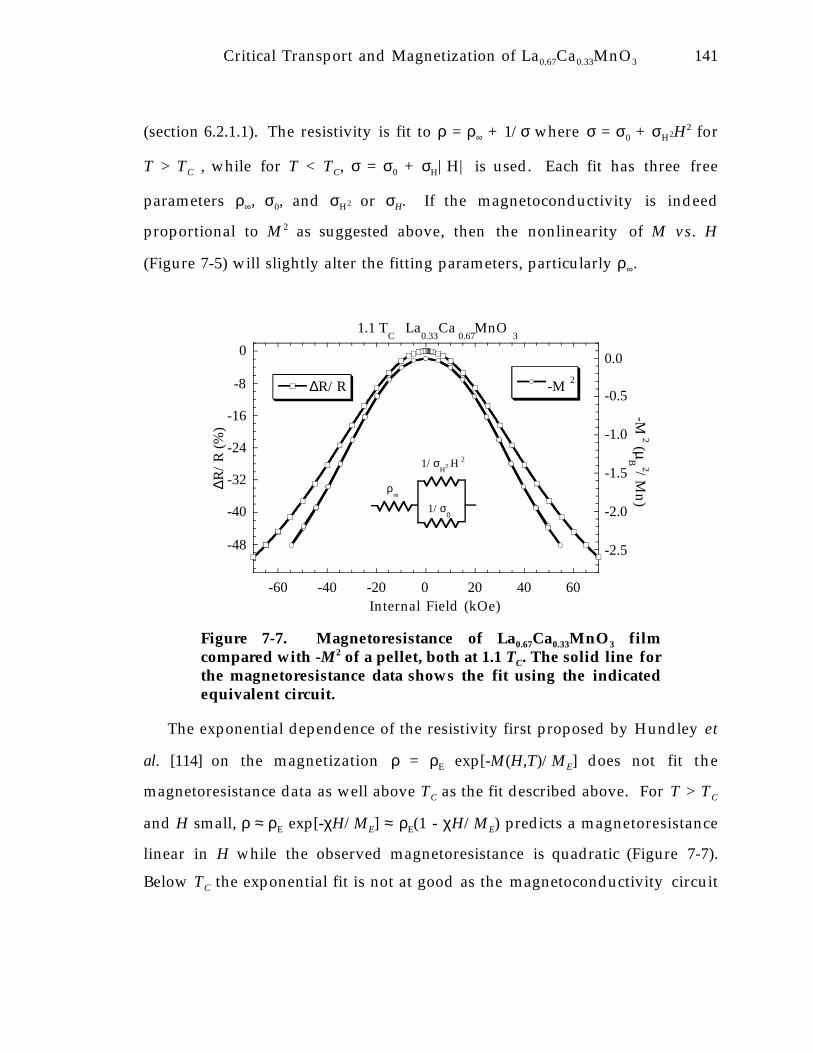
Critical Transport and Magnetization of La0.67Ca0.33MnO3 141

(section 6.2.1.1). The resistivity is fit to ρ = ρ∞ + 1/σ where σ = σ0 + σH2H2 for

T > TC , while for T < TC, σ = σ0 + σH|H| is used. Each fit has three free

parameters ρ∞, σ0, and σH2 or σH. If the magnetoconductivity is indeed

proportional to M2 as suggested above, then the nonlinearity of M vs. H

(Figure 7-5) will slightly alter the fitting parameters, particularly ρ∞.

-48

-40

-32

-24

-16

-8

0

-2.5

-2.0

-1.5

-1.0

-0.5

0.0

-60 -40 -20 0 20 40 60

1.1 TC La

0.33Ca

0.67MnO

3

∆R/R -M 2

∆R/

R (%

)

-M2 (µ

B2/

Mn)

Internal Field (kOe)

ρ∞

1/σ0

1/σH

H 22

Figure 7-7. Magnetoresistance of La0.67Ca0.33MnO3 filmcompared with -M2 of a pellet, both at 1.1 TC. The solid line forthe magnetoresistance data shows the fit using the indicatedequivalent circuit.

The exponential dependence of the resistivity first proposed by Hundley e t

al. [114] on the magnetization ρ = ρE exp[-M(H,T)/ME] does not fit the

magnetoresistance data as well above TC as the fit described above. For T > TC

and H small, ρ ≈ ρE exp[-χH/ME] ≈ ρE(1 - χH/ME) predicts a magnetoresistance

linear in H while the observed magnetoresistance is quadratic (Figure 7-7).

Below TC the exponential fit is not at good as the magnetoconductivity circuit

142 Chapter 7

(Figure 7-6), in so far as the H dependence is concerned; however, the

exponential dependence upon M is found, as will be shown below.

0.0

0.2

0.4

0.6

0.8

1.0

1.2

0.00

0.05

0.10

0.15

0.20

280 290 300 310 320 330

σ0 and ρ

∞ above T

C

ρ∞

σ0

ρ ∞ (

mΩ

cm) σ

0 (mΩ

cm-1)

Temperature (K)

Figure 7-8. Fitting parameters σ0 and ρ∞ for T > TC in aLa0.67Ca0.33MnO3 film. The temperature dependence of thesetwo parameters reflect the insulating behavior of the material.

7. 2. 1 Magnetoresistance scaling above TC

The magnetoresistance data at various temperatures above TC were fit to

the expression ρ = ρ∞ + 1/(σ0 + σH2H2). The resulting parameters σ0 and ρ∞ are

shown in Figure 7-8. The parameter σ0 remains relatively constant, slightly

increasing as expected for a semiconductor. The significance of ρ∞ will be

discussed below.

Critical Transport and Magnetization of La0.67Ca0.33MnO3 143

The parameter σH2, which determines the magnetoresistance, is highly

temperature dependent (Figure 7-9), diverging at TC. The data can be fit with

a critical exponent of -2.0 ± 0.1: σH2(T) = σH2(2TC) (T/TC - 1)-2, where TC = 262 K ±

1 K and σH2(2TC) ≈ 8 × 10-13 Oe-2 mΩcm-1. This result supports an M2

dependence of the magnetoconductance (or magnetoresistance) since

M2 ∝ (T/TC - 1)-2γ above TC, where, as experimentally determined above,

γ ≈ 0.9. Specifically, it is found that σ(H,T) = σ0 + σH2(T)H2 ≈ σ0 + σM2M2. Using

the Curie Weiss susceptibility from [103], M = χH ≈ 5 × 10-4 (emu G-1 cm-3) ×

(T/TC - 1)-1 H, gives σM2 = 3 × 10-6 Oe-2 mΩcm-1.

0.0

0.5

1.0

1.5

2.0

280 300 320 340 360

σ H

(10-1

0 mΩ

cm-1

Oe-2

)

Temperature (K)

2 -26

-25

-24

-23

-22

2.8 3.2 3.6 4.0 4.4ln

(σΗ

)ln(T-262K)

Slope = -2

σΗ

∝ χ 2

Above TC

Resistance ≈ 1/(1+M2)

2

2

Figure 7-9. Fitting parameter σH2 as a function of temperaturein a La0.67Ca0.33MnO3 film for T > TC. The temperaturedependence of σH2 and the square of the susceptibility are thesame, indicating a relationship between themagnetoconductance and M2.

144 Chapter 7

The related form ρ ∝ -M2 would also be consistent with our low field data

since in low fields ∆ρ = -H2 σH2/σ02 and σ0 is nearly constant with respect to

temperature. This form was also observed above TC in La1-xSrxCoO3 [165] and

in small fields for lower TC films [158] of La0.7Ca0.3MnO3. In the temperature

range of this experiment, T > 1.01 TC, 4πM < H, so B = H + 4πM ≈ H and

therefore not very temperature dependent. Thus the resistivity or

conductivity is not proportional to B or B2.

7. 2. 2 Magnetoresistance scaling below TC

Below TC, ρ∞ can be interpreted as due to scattering processes which would

persist if the moments were perfectly ordered. As shown in Figure 7-10, the

resistivity in a infinite field, ρ∞, follows the A + BT2 fit to the low-

temperature, H = 0, intrinsic resistivity described in section 4.2.1. In a true

infinite field (H = ∞) one would expect the resistance to be continuous with a

positive (metallic) slope as T increases through TC. While there is a factor of 2

discrepancy between ρ∞(TC) extrapolated from above (Figure 7-8) and below

(Figure 7-10) this is not unreasonable because two different fitting equations

are used. Particularly above TC, the fitting parameter ρ∞ may not reflect the

true H = ∞ resistivity because the nonlinearity of M upon H is not taken into

account.

The parameter σ0, which can be related to the resistivity in zero field

ρ(H = 0) ≈ ρ∞ + 1/σ0, describes the limiting field-dependent, spin-disorder

scattering processes present as H approaches 0. Unlike ρ∞, 1/σ0 diverges as the

Curie temperature is approached. A critical exponent of about 1.8 (Figure 7-

10) is found: σ0(T) ≈ σ0(0) (1 - T/TC)1.8, where σ0(0) ≈ 2 × 10-3 mΩcm-1.

Critical Transport and Magnetization of La0.67Ca0.33MnO3 145

Figure 7-10. Fitting parameters σ0 and ρ∞ for T < TC in aLa0.67Ca0.33MnO3 film. ρ∞ is governed by the A + BT2 terms inthe resistivity while σ0 diverges at TC. The inset shows σ0 datafit with a (TC - T)1.8 power law (dashed line), and σ ∝exp(M/ME) (solid line). The zero field resistivity ρ(H = 0) =ρ∞ + 1/σ0 is shown for comparison.

The parameter σH is more difficult to interpret than the other parameters.

Although the magnetoresistance, ∆R/HR proportional to σH/σ02, increases as

TC is approached, σH decreases. Thus the large magnetoresistance found

below TC is due to the divergence of 1/σ0 and not σH. The parameter σH does

not always appear to vanish completely as T approaches TC, making it difficult

to fit to a (1 - T/TC)n power law. Assuming TC = 262K (determined from the

critical properties of σH2 and σ0) the exponent for σH is about 0.7.

0.0

0.5

1.0

1.5

2.0

2.5

80 100 120 140 160 180 200 220 240

σ0 and ρ

∞ below T

C

ρ∞

1/σ0

ρ(H = 0)

A + BT2 fit

ρ ∞ a

nd 1

/σ 0 (

mΩ

cm

)

Temperature (K)

-2

-1

0

1

2

3

4

2 3 4 5

ln(σ

0)

ln(262K-T)

σ0 ∝ (T

C-T)1.8

146 Chapter 7

Figure 7-11. Fitting parameter σH as a function of temperaturein a La0.67Ca0.33MnO3 film for T < TC. The solid line shows thebest fit to the data using a critical exponent of 0.7.

There is no simple relationship between either the magnetoconductance

or the magnetoresistance with M2 below TC because the measured scaling

exponents do not agree with those predicted from an M2 dependence as

discussed in the following. Shown in Figure 7-5 is the magnetization below

TC which can be approximated with M(H) = M 0+ χH , and therefore

M2 ≈ M02+ 2χM0H. Assuming σ(H,T) = σ0 + σHH ≈ σM2 M(H,T)2 as suggested

above, then below TC the following relations should hold: σ0 = σM2M02 and

σH = 2χσM2M0. The temperature dependence of M0 and χ below TC should be

governed by the scaling exponents β and γ, via M0 ∝ (1 - T/TC)β and

χ ∝ (1 - T/TC)-γ where experimentally β = 0.3 and γ ≈ 0.9 (typical critical

exponents are β ≈ 0.35 and γ ≈ 1.2). Thus one would expect the critical

0

5

10

15

20

100 150 200 250

σ H (1

0-5 m

Ωcm

-1 O

e-1)

Temperature (K)

-11

-10

-9

3.0 4.0 5.0

ln( σ

H)

ln(262K-T)

Critical Transport and Magnetization of La0.67Ca0.33MnO3 147

exponent for σ0 and σH to be 0.6 and -0.6 respectively. Experimentally,

however σ0 ∝ (1 - T/TC)1.8 and σH ∝ (1 - T/TC)0.7.

An M2 dependence of the magnetoresistance (as opposed to the

magnetoconductance) where ρ ≈ ρ0 - ρMM2 ≈ (ρ0 - ρMM02) - 2ρMχM0H below TC,

is also inconsistent. For low fields ρ = (ρ∞ + 1/σ0) - (σH/σ02)|H| is found

experimentally, which has a field dependent term (σH/σ02), which varies as

(1 - T/TC)-2.9. This is quite different from 2ρMχM0 which has a critical exponent

of β - γ ≈ -0.6.

Below TC, in agreement with previous work [23, 107], the conductivity is

exponentially dependent upon M. Removing the slowly varying

contribution due to ρ∞, this model predicts σ(H,T) = σE exp[M(H,T)/ME] ≈

σ0 + σHH. For H = 0 this reduces to σ0 = σE exp[M0(T)/ME]. The experimental

relationship M0(T) ∝ (1 - T/TC)β with β = 0.3 can be used to fit the magneto-

resistance data. The higher quality of this fit compared to the M2 fit is shown

in Figure 7-10, with ME ≈ 0.4 µB (ME = 1.0 µB in [107]) and σE ≈ 4 × 10-3 mΩcm-1.

An exponential dependence of the conductivity may suggest a tunneling

mechanism is responsible. Tunneling conductivity depends exponentially on

the length of the tunneling barrier. If, in some way, this barrier is decreased

by an increase in the magnetization, then the conductivity will depend

exponentially on M as observed for large M. Spin dependent tunneling is

reported to be the mechanism of the large domain boundary

magnetoresistance observed in these materials [140].

Furthermore, the temperature dependence of σH can also be explained

with the exponential model. According to this model, the field dependent

conductivity σ σ σ σ σ σ σ χH EM M E

E

E

E

d

dH

d

dHe

M

dM

dH ME= = = =/ 0

0 (where

148 Chapter 7

σE exp[M0(T)/ME] ≈ σ0 is used) should have the same temperature dependence

as σ0χ. Experimentally, σ0χ has an approximate temperature dependence of

(1 - T/TC)1.8-0.9, assuming γ ′ (susceptibility exponent for T < TC ) = γ. This is

within experimental error of the critical exponent found (Figure 7-11) for σH

(about 0.7).

7. 2. 3 Magnetoresistance scaling at TC

At or very near TC, the magnetic properties should be described by the

critical exponent δ, where M ∝ H1/δ when T = TC. The magnetoresistance data

for T = 262 K ≈ TC is shown in Figure 7-12, and can be fit to ρ = ρ∞ +

1/(σ0 + σHnHn), where n is an additional free parameter. The data fit well with

n = 1.2 ± 0.1, where the variation of n arises from different ranges and

weighting of the fit. Thus, if at TC, the conductivity σ ∝ M2 then σ ∝ H 2/δ, or

δ = 2/n. This is clearly not the case since 2/n ≈ 1.6 while typically δ ≈ 4.8, or

from the data presented above and the scaling relation δ = 1 + γ/β the value

δ ≈ 4.3 is found.

The T = 262 K data fit well to the composite relation proposed by Sun et al.

[23] σ ∝ M2 exp[M/ME] combined with H = Mδ. Above TC this relation reduces

to σ ∝ M2, which, as was shown above, is quite accurate. Below TC, the

exponential term dominates invalidating the simple σ ∝ M2 relationship.

Critical Transport and Magnetization of La0.67Ca0.33MnO3 149

Figure 7-12. Magnetoresistance of La0.67Ca0.33MnO3 film at 262K ≈ TC. The solid line shows the fit (for the full data on alinear scale) using the indicated equivalent circuit.

7. 2. 4 Relation to low temperature magnetoresistanceThis qualitative correlation between the magnetization and the resistivity

may also account for the intrinsic, small, linear magnetoresistance (Figure 4-

8) found even at the lowest temperatures where the magnetization is nearly

saturated. If at these low temperatures σ = σ0 + σM2M2 then ∆σ/σ (or ∆ρ/ρ) is

given by ∆σ = 2χσM2M0H. Since ∆σ = -∆ρ/ρ2, the susceptibility χ required to

give the observed magnetoresistance is χ = -∆ρ/(2ρ2σM2M0H ) = 2.5 × 10-4

emu/Oe cm3 using the results from chapter 4 for ∆ρ/H = -1.5 × 10-8 mΩcm/Oe,

ρ = 0.125 mΩcm, and M0 = 3.4 µB/Mn = 550 emu/cm3. This is within a factor

of three of the observed value (section 4.2.9, Figure 4-8) χ = 9 × 10-5

emu/Oe cm3. Similarly acceptable, is the exponential model

-80

-70

-60

-50

-40

-30

-20

-10

0

-60 -40 -20 0 20 40 60

262 K ≈ TC La

0.33Ca

0.67MnO

3

∆R/

R (%

)

Field (kOe)

ρ∞

1/σ0

1/σH

Hnn

n = 1.3

150 Chapter 7

σ = σE exp[M(H,T)/ME], which gives at low T and H,

∆ρ/H = -χexp[-M0/ME]/MEσE; requiring χ = 32.9 × 10-5 emu/Oe cm3. A mag-

netoresistive model ρ = (ρ∞ + 1/σ0) - (σM2/σ02)M2 giving ∆ρ = -2χσM2M0H /σ0

2 is

significantly worse since it would predict χ = -∆ρσ02/(2σM2M0H ) = 2 × 10-7

emu/Oe cm3.

In a similar manner, the correlation between the magnetization and the

resistivity should contribute to the T2 contribution (section 4.2.1.2) to the low

temperature resistivity ρ = R0 + R2T2 + … . This is because the magnetization

can be approximated with M = M0(1 - (T/Θ)2) for these temperatures (where

Θ ≈ 500 K, section 4.1.1), giving ρ(T) ∝ -M(T) ∝ T2. For the σ = σ0 + σM2M2

model ρ(T) - ρ(0) = -ρ2(σ(T) - σ(0)) = 2σM2ρ2M02(T/Θ)2 ≈ 1.26 × 10-7 mΩcm K-2 T2.

For the ρ = exp[-M(H,T)/ME]/σE model ρ(T) - ρ(0) = exp[-M0/ME]/σE ×

(T/Θ)2M0/ME ≈ 1.14 × 10-6 mΩcm K-2 T2. Both of these proposed contributions

are less than the observed value (section 4.2.1.2) R2 ≈ 1.96 × 10-5 mΩcm K-2,

suggesting that scattering mechanisms such as electron-electron, or electron-

magnon scattering dominates the R2T2 term.

7.3 ConclusionA scaling relation has been found that satisfactorily characterizes the

magnetic and magnetoresistive properties of La0.67Ca0.33MnO3 near TC.

However the scaling exponents, particularly γ < 1, show that critical scaling

has not been reached even though the measurements reach 0.01 T/TC where

simple ferromagnets are expected to exhibit critical scaling.

An unusual positive nonlinear magnetic susceptibility, which does not

disrupt the scaling, is also observed. The positive non-linear susceptibility

and susceptibility exponent γ < 1 may result from the coupling of the

Critical Transport and Magnetization of La0.67Ca0.33MnO3 151

ferromagnetic and metal-insulator transitions, making the exchange J a

function of M.

The scaling of both the H and T dependence of the magnetoconductance

above TC is consistent with a simple M2 dependence of the conductivity.

However, below or very near TC this correlation predicts the observed H

dependence but can not account for the T dependence. To fit these data, the

model for the magnetoresistance needs to have an exponential dependence

on the magnetization for large M, which reduces to M2 for small M , such as

that previously suggested by Sun et al. [23] σ ∝ M2 exp[M/ME].

152

Appendix A. Critical Behavior and Anisotropy in Single

Crystal SrRuO3

Introduction

Strontium ruthenate, SrRuO3, has many physical properties which make

it unique among perovskite oxides. First, it is metallic in the undoped state

[36, 126, 173-176]. This is even more unusual since the ruthenium in SrRuO3

is in a high oxidation state; whereas many other metallic perovskites must be

formed in reducing environments and therefore unstable in air at high

temperatures. The remarkable chemical stability and simple chemical

formula makes metallic SrRuO3 quite attractive for use in epitaxial thin film

heterostructures with other perovskite oxides when metallic layers are

desired. Indeed, the nearly cubic SrRuO3 [177] is often preferred over the

more distorted CaRuO3 when making structures such as electrodes for

ferroelectrics or superconductor-normal metal-superconductor junctions.

The other striking feature of SrRuO3 is its ferromagnetism with a

reasonably high transition temperature (163 K) and large saturation moment

(> 1µB) [174, 175, 178, 179]. SrRuO3 is the only ferromagnetic perovskite oxide

of a 4d or 5d transition metal. Moreover, SrRuO3 has the largest saturation

moment known to arise from 4d electrons, making it more related to the iron

group ferromagnetic metals (Fe, Co and Ni) than to the weak itinerant

electron ferromagnets such as ZrZn2. SrRuO3 also has very strong cubic

magnetic anisotropy, requiring magnetic fields in excess of 10 Tesla to saturate

the magnetization in the hard directions. Such a strong anisotropy makes

measuring even the simplest properties, such as saturation magnetization,

difficult. It is the purpose of the present work to determine the magnetic

properties of SrRuO3 by measurements of magnetically-soft single crystals

along the easy magnetic direction.

Critical Behavior and Anisotropy in Single Crystal SrRuO3 153

There have been several studies of SrRuO3 in the past three decades,

mostly on polycrystalline samples which are quite easy to prepare. SrRuO3

has a very slightly distorted (GdFeO3 type) perovskite structure. The

deviation from perfect cubic perovskite is so small that it has often been

undetected. The resistivity of polycrystalline, and epitaxial thin film SrRuO3

shows a cusp in dρ/dT at the ferromagnetic Curie temperature TC. This is

commonly observed for metallic ferromagnets and is attributed to spin

disorder scattering [125]. Reported TC's tend to vary from 150K to 165K.

The saturation magnetization of SrRuO3 has been both difficult to

measure and interpret. Low spin Ru4+ in an octahedral coordination has four

4d electrons in the t2g triply degenerate state, giving two paired and two

unpaired electrons. Since the orbital component of angular momentum J

will be quenched, J = S = 1 is expected. The measured Curie constant of the

paramagnetic state is consistent with this model (expected: µeff = √2gJ(J + 1) µB

= 2.83 µB; measured = 2.67 µB [175]). For a localized moment ferromagnet, the

saturation magnetization MS is predicted to be MS = gJ µB = 2.0 µB for SrRuO3.

Measured values of MS are much less. Polycrystalline SrRuO3 reaches about

0.85 µB [175, 178, 179] in low fields but continues to increase in higher

magnetic fields. At 125 kOe it was noted that M had reached 1.55 µB but had

not yet saturated [178]. Early neutron diffraction derived a moment of 1.4 ±

0.4 µB [178] with no evidence for any antiferromagnetic order (spin canting).

Recent theoretical investigations predict incomplete band splitting and a large

moment of about 1.6 µB [176, 180]. Early explanations for the low value of MS

included spin canting, band magnetism, and incomplete alignment of the

magnetization due to magnetocrystalline anisotropy [178]. The present work

shows that SrRuO3 has a large saturation moment of 1.6 µB as predicted by

these calculations.

Single crystals of SrRuO3 can be grown from a SrCl2 flux [36]. The

resistivity of such crystals is consistent with the results on polycrystalline

154 Appendix A

samples. Magnetization and magnetic torque measurements of single crystals

[181-183] showed that SrRuO3 has a high cubic anisotropy with ⟨110⟩ (cubic

cell) being the easy direction, with nearly square hysteresis loops. Some

previous measurements reported for single crystals are questionable, for

example, the measured value of MS = 1.1 µB. In this work new magnetization

data is shown to clarify these points.

Experimental

Single crystals of SrRuO3 were grown by slow cooling in a SrCl2 flux [36,

184]. Polycrystalline SrRuO3 was prepared from stoichiometric quantities of

SrCO3 and Ru metal repeatedly reacted at 1260°C, and was used as the source

material for crystal growth. The SrCl2 was dried in air at 110°C. A mixture

with approximate weight ratio 1:20 of SrRuO3:SrCl2 was melted in a platinum

crucible with lid at 1260°C for 94 hrs. The sample was cooled to 800°C at 1°/hr

and then to room temperature at ~40°/hr. Crystals of SrRuO3 less than 1 m m

in diameter were found at the bottom of the crucible after removing the flux

with water. Most crystals were cubo-octahedron shaped and grew with a

3-fold symmetric axis (presumably [111]) perpendicular to the Pt surface. The

(cubic) crystal orientation was determined by the symmetry of the faces. The

actual orthorhombic symmetry [177] was confirmed by powder x-ray

diffraction and Transmission Electron Microscopy.

Magnetization in fields up to 70 kOe was measured using a Quantum

Design MPMSR2 SQUID magnetometer. The samples were attached to a

plastic straw with a small amount of Apiezon N vacuum grease. Samples

were oriented on the straw visually using crystal faces which had obvious 2-,

3- and 4-fold rotational symmetry. At room temperature, the crystal can

rotate in a large field to align a paramagnetic easy direction with the field.

This was used as a final adjustment when aligning along the easy ⟨110⟩

Critical Behavior and Anisotropy in Single Crystal SrRuO3 155

directions. At low temperatures, the grease solidifies so the sample cannot

rotate. The accuracy of the magnetization measurement was estimated by

measuring a sphere of yttrium iron garnet described in section 3.2.1.1. For the

measure-ments reported here, the sample holder was fixed at the rotation

angle which gave the maximum magnetization. Several crystals were

measured.

Results

Figure A- 1 shows hysteresis loops at 5 K for SrRuO3 single crystal i n

various crystallographic directions and a polycrystalline pellet. The crystals

have a low coercive field (≈ 10 Oe) compared to that of the polycrystalline

pellet (3000 Oe). But more importantly, the crystals show very little hysteresis

1.1

1.2

1.3

1.4

1.5

1.6

1.7

0 10 20 30 40 50 60 70

SrRuO3 Single Crystal

[110][1-10][101][111][100]M

agne

tic

Mom

ent

(µB

/R

u)

Magnetic Field (kOersted)

√(2/3) MS

MS/√2

MS

-2

-1

0

1

2

-75 -50 -25 0 25 50 75

Pellet

M (

µ B/R

u)

H (kOe)

Figure A- 1. Magnetization at 5 K of SrRuO3 single crystalalong several crystallographic directions showing strong cubicbut not uniaxial magnetocrystalline anisotropy. Inset showsthe full hysteresis loop of the single crystal data along withthat of a polycrystalline pellet for comparison.

156 Appendix A

while the pellet displays noticeable hysteresis even in fields greater than

40 kOe.

The rapid, linear approach to saturation (with respect to the applied field)

found in all directions can be attributed to demagnetization. Until the sample

becomes fully magnetized, the demagnetization field Hd is equal to the

applied field Ha resulting in an internal field of zero (Hi = Ha - Hd). From this

slope (M = Ha/4πN), one can calculate the demagnetization factor N and

therefore calculate the internal field. The measured demagnetization factors

N, (Hd = 4πNM) are 0.25, 0.28, 0.31, 0.49, 0.66 for the [110], [1-10], [101], [100] and

[111] directions respectively. These seem reasonable considering the shape of

the crystals. Since a uniaxial magnetocrystalline anisotropy will also give a

linear increase in M if H is applied along the hard direction, it is difficult to

distinguish it from the effect of the demagnetization field in this study. Since

the demagnetization field can be as large as a thousand Oersted, one can only

conclude that the uniaxial anisotropy field is less than a thousand Oersted,

which is considerably less than that ( > 50 kOe) reported previously [182].

In the [110] direction SrRuO3 rapidly approaches saturation and then

remains relatively constant (square hysteresis loop), as is expected for a

magnet with a magnetic field along the easy direction. The crystal was also

measured in the [1-10] and [101] directions which would be equivalent by

symmetry to the [110] if the crystals were cubic. Since the magnetization is the

same along these ⟨110⟩ type directions, it can be concluded that the magnetic

properties of single crystal SrRuO3 are essentially cubic, i.e. only cubic

magnetocrystalline anisotropy is detected. Beyond this initial saturation

along the easy ⟨110⟩ directions, there is a small but measurable increase in the

magnetization which is linear in magnetic field and has a slope of 6 × 10-7

µB/Oe.

Critical Behavior and Anisotropy in Single Crystal SrRuO3 157

The H = 0, T = 0 saturation moment MS found along the easy ⟨110⟩

directions are about 1.62 µB/Ru. In the remnant state (H reduced to zero), the

magnetization should lie along the nearest easy direction. Thus the expected

remnant (H = 0) magnetization along the [100] or [111] direction is simply the

cosine of the angle it makes with the closest ⟨110⟩ direction. For ⟨100⟩ the

expected remnant magnetization is MS/√2, and for ⟨111⟩ directions √(2/3)MS is

expected. These are extremely close to the experimental values (Figure A- 1).

In the other primary directions, there is a nonlinear approach to satur-

ation which is characteristic of materials with cubic anisotropy. The magneto-

crystalline anisotropy constants K1 and K2 can be estimated from these

magnetization curves [185]. The magnetocrystalline anisotropy energy E can

be defined in terms of the cosine of the angle M makes with the three crystal

axes: α i = xi • M/M. For a cubic material E = K1 (α 12α 2

2 + α 22α 3

2 + α 32α 1

2) +

0.0

0.2

0.4

0.6

0.8

1.0

0 5000 10000 15000 20000 25000 30000

SrRuO3 Crystal Arrott Plot

M2 (µ

B2 )

H/M (Oe/µB)

140K

145K

152K

156K

158K

160K162K

163K = Tc164K

166K168K 170K

1

2

3

4

-0.9 -0.8 -0.7 -0.6 -0.5 -0.4 -0.3

T = 163K H ∝ Mδ

Log

(H)

Log(M)

δ = 4.2(1)

Figure A- 2. Arrott Plot of SrRuO3 single crystal along easy[110] direction. Inset, critical isotherm (T = 163K ≈ TC) on a logscale fit to Mδ ∝ H with δ = 4.2.

158 Appendix A

K2 (α12α2

2α32) + … . In SrRuO3 the magnetic easy axes are ⟨110⟩ , which requires

K1 < 0. Similarly, ⟨100⟩ are the hard axes (⟨111⟩ are intermediate) which

implies 2.25|K1| < K2 < 9|K1|. The [100] magnetization should intersect that

of the easy axis [110] at Ha = -2K1/MS. An extrapolation of the [100] M vs. H

curve gives -2K1/MS ≈ 109 kOe. Alternatively, the area between the [100] and

the [110] M vs. H curves should be equal to -K1/4. This method gives a value

for -2K1/MS ≈ 96 kOe. The area method can also be used with the [111] curve

to estimate 2K2/MS ≈ 540 kOe.

In the easy [110] direction, M vs. H curves were measured for various tem-

peratures and are shown in Figure A- 2 as M2 vs. H/M (Arrott plot). The iso-

therms below TC should be approximately linear and intersect H/M = 0 at M0.

0.0

0.2

0.4

0.6

0.8

1.0

125 130 135 140 145 150 155 160 165

SrRuO3 M

0 ∝ (T

C-T)β

M0 (µ

B)

Temperature (K)

Average β = 0.36T

C = 163.2(1) K

-0.5

-0.4

-0.3

-0.2

-0.2

-0.1

0.0

0 0.2 0.4 0.6 0.8 1 1.2 1.4 1.6

Log

(M0)

Log(TC

-T)

β = 0.32T far from T

C

β = 0.39T near T

C

Figure A- 3. Zero field magnetization M0 of SrRuO3 singlecrystal along easy [110] direction. Solid line shows the fit toM0(T) ∝ (1 - T/TC)β with β = 0.36. Inset showing the same dataon a log plot. The critical exponent β appears to change fromHeisenberg-like β = 0.39 near TC to Ising-like β = 0.32 as Tdecreases.

Critical Behavior and Anisotropy in Single Crystal SrRuO3 159

From these M0(T), shown in Figure A- 3, the critical exponent β ≈ 0.36 and

TC = 163.2 ± 0.2 K can be estimated by fitting M0(T) ∝ (1 - T/TC)β in the critical

region. The fit with a single value for β = 0.36 is poor considering the

apparent precision of the data. Closer to TC, the data fit better with a larger

β ≈ 0.39 which is close to that predicted in the 3-d Heisenberg model (β = 0.38).

Farther from TC, the exponent is smaller, β ≈ 0.32, near that predicted by the

Ising model (β = 0.33). It is possible that this is due to a crossover from

Heisenberg to Ising behavior at T decreases from TC. A similar model has

been proposed to explain measurements of thin film SrRuO3 [73].

The T > TC isotherms of Figure A- 2 should intersect M2 = 0 at

1/χ(T, H = 0) = 1/χ0. The critical exponent γ is then found from 1/χ0 ∝

0

5

10

15

20

25

160 165 170 175 180 185 190 195

SrRuO3 Crystal Inverse Susceptibility

1/χ 0 (

emu-1

mol

Gau

ss)

Temperature (K)

3.0

3.5

4.0

4.5

5.0

0 0.5 1 1.5L

og(1

/χ 0)

Log(T-TC

)

χ0 ∝ (T-T

C)- γ

γ = 1.17

0

50

100

150

200

150 200 250 300 350

PelletSingle Crystal

1/χ 0 (

emu-1

mol

Gau

ss)

Temperature (K)

Figure A- 4. Zero field inverse susceptibility 1/χ 0 of SrRuO3

single crystal along easy [110] direction. Solid line shows thefit to 1/χ0(T) ∝ (1 - T/TC)γ with γ = 1.17 and TC = 163.2 K. Theinset shows the same data on a log plot.

160 Appendix A

(T/TC - 1)γ. From these data (Figure A- 4) γ = 1.17 ± 0.02 is estimated. The plot

of 1/χ vs. T should be close to linear for high temperatures.

The M(H, T) data can be replotted using the scaling hypothesis [90] with

β = 0.36 and γ = 1.17. According to the hypothesis, the magnetic equation of

state in the critical region depends only on the scaled variables H/|TC/T - 1|β+γ

and M/|TC/T - 1|β. A plot of the scaled M2 and scaled H/M, shown i n

Figure A- 5, will then have only two curves: one branch for the T < TC data

and another for T > TC. Not all the curves fit on a single line, this is due to

the apparent change in β as discussed above.

The critical isotherm (T = TC) should obey the relation Mδ ∝ H, where

according to the scaling relation δ = γ/β + 1. From the previously measured

values of β and γ, the exponent δ is therefore expected to be 4.3 ± 0.5. This is

in good agreement with the measured value (Figure A- 2) δ = 4.2 ± 0.2.

0.0

1.0

2.0

3.0

4.0

5.0

6.0

0 500 1000 1500 2000 2500

SrRuO3 Crystal Scaled Arrott Plot

M2 ×

|T

/T

C - 1|

-2β (µ

B

2 )

H/M × |T/TC

- 1|-γ (kOe/µB)

T < TC

T > TC

β = 0.36γ = 1.17

TC=163.2K

Figure A- 5. Scaled Arrott Plot of SrRuO3 single crystal alongeasy [110] direction with β = 0.36 and γ =1.17. Symbols are thesame as those used in Figure A- 2.

Critical Behavior and Anisotropy in Single Crystal SrRuO3 161

The temperature dependence of M along the easy direction is shown i n

Figure A- 6 for various applied fields. The demagnetization field of 4πNM ≈

800 Oe should be subtracted from the applied field to give the internal field.

Between 5 K and 100 K, and for internal fields from 0.2 kOe to 68 kOe the

magnetization is well approximated by M = M0(1 - (T/Θ2)2) where M0 and Θ2

are fitting parameters. Other possible analyses are discussed below.

Discussion

The low temperature magnetization data (Figure A- 1) of bulk SrRuO3 can

be explained with ⟨110⟩ easy directions and a large cubic, but very little

uniaxial, magnetocrystalline anisotropy. The low coercivity of the crystals

(~10 Oe), compared to the 3 kOe coercivity found in polycrystalline samples,

1.30

1.35

1.40

1.45

1.50

1.55

1.60

1.65

0 10 20 30 40 50 60 70 80 90 100

SrRuO3 Single Crystal along easy direction [110]

7T6T5T4T3T

2T1T2kG1kG

Mag

neti

zati

on (

µ B/

Ru)

Temperature (K)

1.3

1.4

1.5

1.6

1.7

0 2000 4000 6000 8000 10000

M (

µ B/

Ru)

T2 (K2)

Figure A- 6. Magnetization as a function of temperature ofSrRuO3 single crystal along easy [110] direction. Inset showsthe approximate T2 dependence of the magnetization.

162 Appendix A

provides highly reversible and square hysteresis curves. There is no

indication of a magnetic multi-domain structure [183].

The cubic magnetocrystalline anisotropy in SrRuO3 is very large, as

reported previously [181, 183]. Typical values of K1 for cubic 3-d ferromagnets

are 100 times smaller than that found for SrRuO3. Such large values of K1

usually refer to uniaxial anisotropy, for instance in hexagonal materials,

which is a lower order effect (K1 refers to the first non-zero anisotropy

constant). This large anisotropy probably results from the strong spin-orbit

coupling of the heavy Ru atom, which also gives SrRuO3 a strong Kerr effect

[186].

From measurements along different ⟨110⟩ directions, no indication of

uniaxial magnetocrystalline anisotropy [182] is found, although it is allowed

from the orthorhombic symmetry. This might be expected since the

crystallographic unit cell lengths [177] vary by only 0.03%, and the angles by

0.4% from the perfect cubic ones. The distortion from cubic is primarily due

to a rotation of the RuO6 octahedra, which alters the symmetry much more

than the shape of the unit cell [177]. In the crystals reported here, the

orthorhombic cell was confirmed using TEM. Because the unit cell is only

slightly distorted, the few reports claiming cubic [184] or tetragonal [182]

crystallographic symmetry without supporting evidence, should be

reevaluated in this context. Significant uniaxial anisotropy reported in thin

films of SrRuO3 [187] may result from growth induced anisotropy, as was

found in films of magnetic garnets used in magnetic bubble technology [188].

Due to the large magnetocrystalline anisotropy, the saturation moment

of SrRuO3 is difficult to measure. In directions other than ⟨110⟩ the magnetic

moment does not saturate even in fields of several 10 kOe. The strain and

small particle size of a polycrystalline sample apparently makes it even more

difficult to saturate than the hard direction in a single crystal (Figure A- 1).

Polycrystalline SrRuO3 has a remnant magnetization (H = 0) of MS ≈ 0.85 µB,

Critical Behavior and Anisotropy in Single Crystal SrRuO3 163

which increases non-linearly past 1.55 µB (H = 125 kOe) [178]. Clearly a

magnetically soft single crystal with H along the easy direction is needed to

measure MS. In a previous experiment [181] on single crystal SrRuO3 with a

square hysteresis loop, MS = 1.1 µB at H = 0 was reported. However, that value

of MS is clearly too small since by 17 kOe it is smaller than the value for a

polycrystalline sample [181]. Our measured value of MS = 1.6 µB (H = 0) is

consistent with the high field polycrystalline results.

The magnetic critical exponents measured here are in the range typically

seen in large moment ferromagnets and expected theoretically for 3-

dimensional ferromagnets. Experimental values for the critical exponent β in

Fe, Ni and YIG [92] are 0.37 ± 0.02, which are near the theoretical values (Ising

β = 0.33, Heisenberg β = 0.36). The related metallic ferromagnets La0.5Sr0.5CoO3

[92] has β = 0.361. The apparent decrease in β as T decreases from TC, may be

due to the large magnetocrystalline anisotropy. A similar effect has been seen

in thin film SrRuO3 [187], where it is suggested that the magnetocrystalline

anisotropy induces a crossover from Heisenberg to Ising behavior. The weak,

itinerant electron ferromagnet ZrZn2 has mean field critical exponents β = 0.5

[93]. The most prominent theory on itinerant electron ferromagnetism by

Moriya [84, 85] predicts a TC4/3 - T4/3 dependence on the magnetization, which

is essentially β = 1.

The critical exponents γ and δ are also typical for large moment

ferromagnets (Fe, Ni and YIG [92] γ = 1.2 ± 0.2) as opposed to those found for

the weak, itinerant electron ferromagnet ZrZn2 which has mean field critical

exponents γ = 1.0 and δ = 3 [93]. The three dimensional Ising and Heisenberg

models predict γ = 1.24, δ = 4.8 and γ = 1.39, δ = 4.8 respectively. The critical

exponents measured here also obey the scaling relation δ = 1 + γ/β.

164 Appendix A

A positive curvature persists in the plot of 1/χ vs. T (Figure A- 7) even at

higher temperature where it should be linear for a Curie-Weiss ferromagnet.

Such a curvature can be caused by a temperature independent term in the

susceptibility χ = χConst + C/(T - Θ), where C/(T - Θ) is the Curie-Weiss

susceptibility and is always positive (T > Θ). A χConst < 0 of about -4 × 10-4 emu

G-1 mol-1 will provide the observed curvature, and has been independently

observed elsewhere [175]. The temperature independent term χConst, should

contain a positive contribution due to Pauli paramagnetism. This can be

estimated from measurements of the linear term of the specific heat [176],

giving χPauli ≈ +4 × 10-4 emu G-1 mol-1. The Landau diamagnetism should be

0

50

100

150

200

150 200 250 300 350

SrRuO3 Polycrystal Inverse Susceptibility

PelletSingle Crystal

Temperature (K)

1/χ 0 (

emu

-1 m

ol G

auss

)

Figure A- 7. Inverse magnetic susceptibility (1/χ = M /H) at H= 10 kOe of polycrystalline SrRuO3 compared to the singlecrystal data from Figure A- 4. The solid line is the straight-line fit with TC = 165K which demonstrates the slightlypositive curvature of the data.

Critical Behavior and Anisotropy in Single Crystal SrRuO3 165

negative and for simple band structures is smaller than χPauli (for free electrons

χLandau = -χPauli/3). The core diamagnetism can be estimated from tables of

experimental values [76] giving χCore = -0.7 × 10-4 emu G-1 mol-1. The sum of

these theoretical estimates χConst = χPauli + χLandau + χCore is, however, still

positive while the experimental value appears to be negative. In the critical

region, 1/χ ∝ (T/TC - 1)γ with γ = 1.17, provides a positive curvature in the plot

of 1/χ vs. T. Since the mean field exponent γ = 1 is expected to be valid far

from TC, some other mechanism must provide the effective γ > 1 observed at

these higher temperatures.

Magnetic excitations which become thermally induced as the temperature

is raised above T = 0 reduce the magnetization from the ground state value.

The exponential decrease predicted by the mean field model has some

qualitative value but is never in good agreement with experiment. Collective

spin wave excitations and single particle (Stoner) excitations both decrease the

magnetization according to a power law M = MS(1 - (T/Θn)n) which is in accord

with experiments where n ≈ 2 ± 1 and Θn is of the order TC.

The limiting low T, H = 0 behavior of collective, spin wave excitations

(section 3.2.2.2.8) predicts n = 3/2 and for SrRuO3, Θ3/2 ≈ 2.42TC = 400 K. The

Stoner theory of single (k-space) particle excitations (section 3.2.2.2.2) predicts

n = 2 and Θ2 ≈ 1.41 TC (= 230 K for SrRuO3). As the temperature and magnetic

field is raised, these models require further corrections. For example, higher

order corrections such as an additional n = 5/2 term in predicted in the spin

wave theory. For H ≠ 0, the low temperature spin-wave excitations become

quenched which can have the effect of increasing the average value on n [97].

The generalized model of spin fluctuations in ferromagnets ([84] section

166 Appendix A

3.2.2.2.3) includes both types of interacting magnetic excitations and predicts

n = 3/2 for H = 0, T = 0 but also n ≈ 2 in calculations [86].

Experimental results on metallic ferromagnets with substantial saturation

moments such as Fe, Ni [88, 189-192] and La0.67Sr0.33MnO3 ([97], section 4.1.1)

can display n = 3/2 consistent with the spin wave stiffness determined by

neutron diffraction if significant corrections are included and only low

temperature data is analyzed. In contrast “weak” itinerant-electron

-50

0

50

100

150

200

0 25 50 75 100 125 150

A parameter in fit to M = MS(1 - AT3/2 - BT2)

T3/

2 Coe

ffic

ient

(10

-6/

K3/

2 )

Maximum Temperature of Fitting Range

-20 0 20 40 60 8010

15

20

25

Correlation of A and B

T3/2

Coefficient (10-6

/K3/2

)

T2 C

oeff

icie

nt (

10-6

/K

2 )

Figure A- 8. Variation of the T3/2 parameter in fitting themagnetization data of single crystal SrRuO3 to M = MS (1 -AT3/2 - BT2) as the fitting range is increased. The upper insetshows the correlation of the A and B parameters. In theregion where A is relatively stable (around Tmax = 60 K), Adecreases as Tmax is lowered. The symbols are the same asthose used in Figure A- 9.

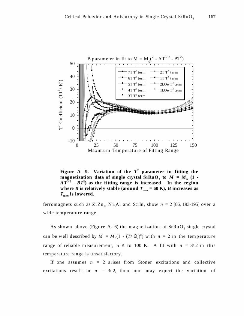
Critical Behavior and Anisotropy in Single Crystal SrRuO3 167

ferromagnets such as ZrZn2, Ni3Al and Sc3In, show n = 2 [86, 193-195] over a

wide temperature range.

As shown above (Figure A- 6) the magnetization of SrRuO3 single crystal

can be well described by M = MS(1 - (T/Θn)n) with n = 2 in the temperature

range of reliable measurement, 5 K to 100 K. A fit with n = 3/2 in this

temperature range is unsatisfactory.

If one assumes n = 2 arises from Stoner excitations and collective

excitations result in n = 3/2, then one may expect the variation of

-10

0

10

20

30

40

50

0 25 50 75 100 125 150

B parameter in fit to M = M0(1 - AT3/2 - BT2)

7T T2 term

6T T2 term

5T T2 term

4T T2 term3T T2 term

2T T2 term

1T T2 term

2kOe T2 term

1kOe T2 term

T2 C

oeff

icie

nt (

10-6

/K

2 )

Maximum Temperature of Fitting Range

Figure A- 9. Variation of the T2 parameter in fitting themagnetization data of single crystal SrRuO3 to M = MS (1 -AT3/2 - BT2) as the fitting range is increased. In the regionwhere B is relatively stable (around Tmax = 60 K), B increases asTmax is lowered.

168 Appendix A

magnetization with temperature to fit with a combination of the n = 2 and

n = 3/2 terms, M = MS (1 - AT3/2 - BT2) [150] at low temperatures. Since an

additional parameter is included, an improvement of the fit does not

necessarily prove the significance of the added parameter. Furthermore, the

functions T3/2 and T2 are very similar making the fitting parameters highly

correlated.

The magnetization data for single crystal SrRuO3 were fit to a polynomial

expression M = MS (1 - AT3/2 - BT2) from T = 2 K to T = Tmax. As expected, the A

and B parameters are highly correlated (Figure A- 8) with ∆B ≈ 2.2 × 10-5 K-2 -

0.2 K-1/2 ∆A. The parameters A and B can then be plotted as a function of Tmax

(Figure A- 8 and Figure A - 9). For very low Tmax (< 30 K) the fit is unstable

since the difference in the magnetization at T <Tmax becomes comparable to

precision of the measurement. Thus, the divergence of the fitting parameters

at low Tmax is an artifact, and not physical. At high temperatures, nearing the

critical temperature, the polynomial expression is not expected to be valid, so

the divergence at high Tmax can also be ignored. The flat, linear region

centered around Tmax = 60K, is presumably the region where the fitting

parameters may have physical meaning. From this region, A and B

parameters can be extracted and extrapolated to the Tmax = 0 K values for

comparison with the theory. This analysis was done for fitting the

magnetization data both to M = MS (1 - AT3/2 - BT2) and M = MS (1 - BT2).

Implicit in the use of M = MS (1 - AT3/2 - BT2) is the assumption that these

two terms are theoretical low temperature expansions, i.e. they should

become more accurate as T approaches 0 K. As the temperature range for

which the data is fit to this type of expression is decreased to lower

temperatures, the fitting parameters should be stable, or only be slightly

varying. In principle, the true low temperature form should gradually

become more dominant, at the expense of the other terms, as the fitting range

is decreased to lower temperatures.

Critical Behavior and Anisotropy in Single Crystal SrRuO3 169

In fitting to the data on SrRuO3 single crystal the B parameter (Figure A-9)

is relatively stable and increases as lower temperature fitting ranges (Tmax) are

used. The A parameter (Figure A- 8) is not as stable and appears to decrease as

Tmax is lowered. If this trend were to continue, then the T3/2 contribution

would be very small at low temperatures. The removal of the AT3/2 term

further stabilizes the B parameter (Figure A- 10), and makes B more

independent of Tmax than with AT3/2 included. Thus, from this analysis of the

magnetization data, there is little evidence for a large AT3/2 contribution to

the magnetization. This is in contrast with measurements on thin film [186,

187] which show T3/2 dominating over T2.

The two corrections to the spin wave T3/2 theory mentioned above (finite

magnetic field and higher order T(2n+1)/2 terms) may not adequately explain the

data presented here. The applied magnetic field will suppress spin wave

-10

0

10

20

30

40

50

0 25 50 75 100 125 150

B parameter in fit to M = M0(1 - BT2)

T2 C

oeff

icie

nt (

10-6

/K

2 )

Maximum Temperature of Fitting Range

210

215

220

225

230

235

240

0 1 2 3 4 5 6 7

Θ2 (T

max = 60K)

Θ2 (

K)

Internal Field (T)

233K = √2TC

expected fromsimple Stoner Theory

Θ2 = B1/2

Figure A- 10. Variation of the T2 parameter in fitting themagnetization data of single crystal SrRuO3 to M = MS (1 - BT2)as the fitting range is increased. The parameter B for this fit ismore stable and constant than that shown in Figure A- 8.Inset, variation of Θ2 in a magnetic field.

170 Appendix A

excitations for T < gµBH/kB, resulting in an effective n > 3/2. If this were a

significant effect, the T3/2 fitting parameter A should decrease as H is increased

particularly as Tmax approaches 0 K. Such a systematic decrease in A is not

obviously apparent (Figure A- 8). One cannot however, exclude the

demagnetization or anisotropy field which are present even when the applied

H = 0.

If the true magnetization were a sum of T3/2 and T5/2 terms, M/MS =

(1 - (T/400 K)3/2 - (T/600 K)5/2 ) for instance, the data would fit well to M/MS =

(1 - AT3/2 - BT2). The fitting parameters A and B as a function of Tmax for this

example are shown in Figure A- 11. The A parameter is relatively constant,

increasing slightly as Tmax approaches 0 K. In the limit Tmax approaches 0 K,

A = 125 × 10-6 K-3/2 or Θ3/2 = 400.3 K, which is very close to the true value of

400 K. The B fitting parameter is not nearly as stable and decreases as Tmax

0

20

40

60

80

100

120

140

0.0

0.5

1.0

1.5

2.0

0 20 40 60 80 100

M = 1 - (T/400 K)3/2 - (T/600 K)5/2

fit with M = MS(1 - AT3/2 - BT2)

A

B

AT

3/2 C

oeff

icie

nt (

10-6

/K

3/2 )

BT

2 Coefficient (10

-6/K

2)

Maximum Temperature (K) of Fitting Range

Figure A- 11. Variation of A and B fitting parameters in thehypothetical case where the true magnetization is given by T3/2

and T5/2 terms.

Critical Behavior and Anisotropy in Single Crystal SrRuO3 171

approaches 0 K. Since the exponent of the BT2 fit (2) is smaller than 5/2,

which is the exponent used in the example, a larger B is needed to fit the data

at higher temperatures. Thus, a dramatically decreasing B as Tmax approaches

0 K, is indicative of a fitting exponent (2 in this example) smaller than the

true exponent (5/2 in this example).

The data on SrRuO3 shows the opposite effect: B is relatively constant

while A decreases as Tmax approaches 0 K. This decrease of A indicates that

the exponent 3/2 is smaller than the true exponent, and therefore, the

addition of higher order terms to the spin wave form of the magnetization

will not fully explain the data on SrRuO3.

Positive B (and A) parameters can be converted to the Θn values used

above via Θ2 = B-1/2 and Θ3/2 = A-2/3. The Θ2 values extracted from fits

described above are shown as a function of the internal magnetic field i n

Figure A- 10. The values of Θ2(H) extrapolated to Tmax = 0 are 20 K less than

the corresponding Θ2(H) for Tmax = 60 K. The single crystal Θ2 parameters

increase only slightly as the field is increased, about 2.6 K/Tesla. These values

for Θ2 are consistent with measurements of the field dependent heat capacity

of polycrystalline SrRuO3 (Figure B- 3) via the Maxwell relation

∂CH

∂H

T

= T∂ 2M

∂T 2

H

.

ConclusionVarious magnetic properties of single crystal SrRuO3 along the magnetic

easy direction have been measured. The saturation moment, 1.61µB/Ru, is

larger than that reported previously for single crystal material but in accord

with experiments on polycrystalline material and theoretical calculations.

The crystals show extremely large cubic magnetocrystalline anisotropy while

no substantial uniaxial magnetocrystalline anisotropy. The critical exponent

172 Appendix A

β changes from Heisenberg like 0.39 near TC to Ising like 0.32 further from TC.

The susceptibility exponent γ = 1.17 persists to 2 TC, where it is expected to

decrease to 1. The magnetization from 5 K to 100 K is well described by

M = MS(1 - (T/Θn)n) where n ≈ 2. The addition of a T3/2 term is not obviously

significant.

173

Appendix B. Magnetic Excitations and Specific Heat in

SrRuO3

Low temperature magnetic excitations can be probed not only by

measurements of the magnetization but also by the heat capacity. As will be

discussed below, the two measurements are related via a Maxwell relation.

SrRuO3 polycrystalline samples were prepared by repeated heating of a R u

and SrCO3 mixture at 1260°C (seciton 2.1.1). Heat capacity data were taken

using the relaxation method [102] (section 3.3). Constant field data were taken

on a zero field cooled sample at 0 and 8 T, and in zero field after the

application of an 8 T field. In addition, data at temperatures between 4 K and

5 K were taken at several intermediate fields.

Specific heat data taken in 0 T and 8 T applied magnetic field are shown i n

Figure B- 1. The zero field cooled and zero field remnant data are equal

within experimental error. Between 3 K and 13 K both the 0 T and 8 T data

appear to be well described by a straight line on this plot of c/T vs. T2,

suggesting that the specific heat can be described by γT+βT3. The parameter

values from fitting the data in zero field are γ = 37 mJ mol-1 K-2and

β = 0.19 mJ mol-1 K-4. This value of β corresponds to a Debye temperature of

371 K and is in good agreement with previous zero-field measurements [176,

196], while γ is about 20% larger than that found previously. The value of γ i n

zero field, 37 mJ mol-1 K-2, is 4.6 times that expected of the bare density of states

given by spin resolved band structure calculations [176]. The effect of

demagnetization fields should be negligible since the correction to the specific

heat is approximately proportional to T3 but only about 0.1% of the measured

value of β [197, 198].

174 Appendix B

Above 13 K and below 3 K the data in Figure B- 1 deviate from a straight

line. The deviation above 13K can be fit by an expression for the specific heat

of a thermally activated Einstein (optical) phonon mode, with an Einstein

temperature of ΘΕ = 140 K. Both β and ΘΕ are field independent within

experimental error. The temperature range below 3 K is not large enough to

draw conclusion about the functional form of the low-temperature upturn.

A field independent term proportional to T3ln(T) is expected from the non-

spinwave spin fluctuations [91, 194, 199]. A Shottky anomaly due to free

30

40

50

60

70

80

90

100

110

0 50 100 150 200 250 300 350

SrRuO3 Specific Heat

0 T zfc0 T rem8 T

c P,H

/T

(mJ/

mol

·K2 )

Temperature 2 (K2)

-5

-4

-3

-2

-1

0

1

0 50 100 150 200 250 300 350

∆cP,

H/

T (

mJ/

mol

·K2)

Temperature 2 (K2)

cP,H

/T (rem) - cP,H

/T (zfc)

cP,H

/T (8T) - cP,H

/T (zfc)

Figure B- 1 Heat capacity of SrRuO3 cooled in zero field (zfc),in an 8 T magnetic field, and in zero field after beingmagnetized (rem). Inset, difference between the heat capacitymeasured after cooling in zero field with that in 8 T and theremnant magnetized state.

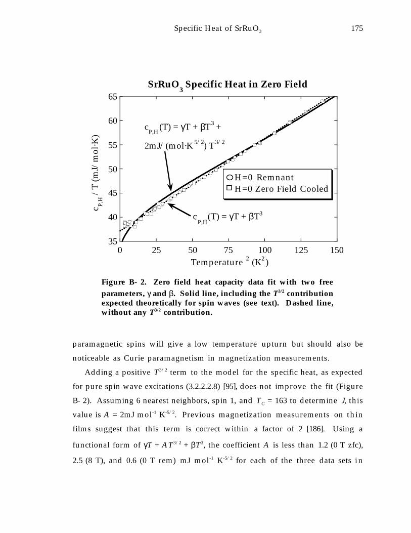
Specific Heat of SrRuO3 175

paramagnetic spins will give a low temperature upturn but should also be

noticeable as Curie paramagnetism in magnetization measurements.

Adding a positive T3/2 term to the model for the specific heat, as expected

for pure spin wave excitations (3.2.2.2.8) [95], does not improve the fit (Figure

B- 2). Assuming 6 nearest neighbors, spin 1, and TC = 163 to determine J, this

value is A = 2mJ mol-1 K-5/2. Previous magnetization measurements on thin

films suggest that this term is correct within a factor of 2 [186]. Using a

functional form of γT + AT3/2 + βT3, the coefficient A is less than 1.2 (0 T zfc),

2.5 (8 T), and 0.6 (0 T rem) mJ mol-1 K-5/2 for each of the three data sets i n

cP,H

(T) = γT + βT3

cP,H

(T) = γT + βT3 +

2mJ/(mol·K 5/2) T3/2

35

40

45

50

55

60

65

0 25 50 75 100 125 150

SrRuO3 Specific Heat in Zero Field

c P,H

/T

(mJ/

mol

·K)

Temperature 2 (K2 )

H=0 RemnantH=0 Zero Field Cooled

Figure B- 2. Zero field heat capacity data fit with two freeparameters, γ and β. Solid line, including the T3/2 contributionexpected theoretically for spin waves (see text). Dashed line,without any T3/2 contribution.

176 Appendix B

Figure 3 at the 90% statistical confidence level. The T3/2 term in Fe and Ni is

quite small but has nevertheless been extracted from the heat capacity data

[200-202].

The linear-T term, γ, is significantly depressed in an 8 T magnetic field.

The inset to Figure B- 1 shows the difference between the zero-field cooled

data in zero field and each of the other two data sets, plotted as ∆c/T. The data

32

33

34

34

35

36

37

38

0 2 4 6 8

Field Dependence of the Density of States in SrRuO3

γ (H

) (m

J/m

ol-K

2 )

Magnetic Field (Tesla)

Predicted from M vs. TSingle Crystal Data

Figure B- 3. The linear term of the heat capacity γ as afunction of magnetic field. Each circle is from a single cP,H

datum between 4.3 and 5 K with phonons subtracted: γ(H) =(cP,H(T) - βT3)/T with β = 0.191 mJ/mol·K4. γ(H) for each squarewas determined by fitting 15-20 data points between 6 and 12 Kto: cP,H(T) = γT + βT3. The triangles are calculated from themagnetization data of a single crystal.

Specific Heat of SrRuO3 177

taken in 0 T after application of an 8 T field (circles) shows that the zero-field

data are not hysteretic. On this plot of ∆c/T, the 8 T data (diamonds) show

that the only observed change in the specific heat is a decrease in the linear-T

term.

To further understand the field dependence of γ, specific heat points

between 4 K and 5 K at several intermediate fields were also taken. These

data are shown in Figure B- 3 (open circles) as γ(H) = (c(T,H) - βT3)/T using the

value of β measured at 0 T and 8 T. On the same plot, the open squares

indicate the fitted value of γ from the three data sets in Figure B- 1.

Figure B- 3 shows that the coefficient of the linear-T term in the specific heat

decreases approximately linearly with applied magnetic field, H.

To summarize, the specific heat between 3 and 13 K can be described by

c(T,H) = (γ - γ H)T+βT3.

Although the magnetization of polycrystalline SrRuO3 is irreversible, the

measured heat capacity is not. Therefore, the heat capacity originates from

processes reversible with respect to a magnetic field, showing that the entropy

associated with random domains is negligible. In this sense, the heat capacity

is a better thermodynamic measure of the low-lying excitations. The

magnetic field dependence of the heat capacity and the magnetization are

related by the following Maxwell relation:

∂CH

∂H

T

= T∂ 2M

∂T 2

H

(1)

According to equation 1, the first derivative of the heat capacity with

respect to field gives information about the second derivative of the

magnetization with respect to temperature. This relation is generally valid

for an isotropic system as long as there are no irreversible processes involved

and no PV work is done. Equation 1 is actually three equations since H and M

178 Appendix B

are vectors. Thus for an ideal, simple experiment, the sample would be very

soft magnetically (no magnetic hysteresis) and the magnetic field would be

aligned in the magnetic easy direction to keep M and H parallel. If possible,

the magnetic and heat capacity experiments should be done on the same

sample in the same direction; although, in principle different samples should

give the same result since both M and CP in a reversible sample should not

depend on the microstructure. In order to use equation 1 to relate the

reversible magnetization from the measured specific heat, it is assumed that

effects due to the field dependence of the magnetocrystalline anisotropy are

insignificant.

The simplest spin wave model (section 3.2.2.2.8) predicts a T3/2 dependence

of the magnetization at low temperatures:

M H T

M H

T

H

( , )( , ) ( )0

132

32

≈ −

Θ

(2)

with Θ3/2 ≈ 2.42TC = 400K [95, 186] for SrRuO3. Corrections due to H ≠ 0 and

T > 0 can also be calculated [95]. The Stoner/Wohlfarth theory of magnetism

(section 3.2.2.2.2) [81] predicts a somewhat different temperature dependence:

M H T

M H

T

H

( , )( , ) ( )0

12

2

≈ −

Θ

(3)

(Θ2 ≈ √2TC = 231K for SrRuO3) due to single (k-space) particle excitations.

The Maxwell relation together with the observed magnetic field

dependence of the specific heat above 4 K, γ ´HT, implies that the second

derivative of the magnetization with respect to temperature, ∂∂

2

2

M

T H

, is a

constant. This result is consistent with the dominant T2 temperature

dependence of the reversible discussed above.

In order to make quantitative comparisons between the specific heat data

and the magnetization data, equation 1 can be integrated with respect to H

Specific Heat of SrRuO3 179

from H = 0 to H = ∆H. Since magnetization data is not available at all fields,

the integral is approximated to a finite sum with step size dH:

∆∆ ∆

∆C T

T H

dH

H

M n dH T

TH

n

H dH( ) ( , )/

≈ ⋅=

−

∑ ∂∂

2

20

1

(4)

where ∆CH(T)=CH(T,H=∆H)-CH(T,H=0). The two simplest physically plausible

temperature dependencies of the reversible magnetization, T2 (equation 3) or

T3/2 (equation 2), each correspond to a simple temperature dependence of

∆∆

C T

T HH ( )

:

M H T

M H

T

H

C T

T H

dH

H

M n dH

n dHConstH

n

H dH( , )( , ) ( )

( ) ( , )( )

./

01

2 00

2

2

22

0

1

≈ −

⇒ = − ⋅⋅

= <=

−

∑Θ∆

∆ ∆ Θ

∆

(5)

M H T

M H

T

H

C T

T H

dH

T H

M n dH

n dH TH

n

H dH( , )( , ) ( )

( ) ( , )( )

/

01

34

0 1

32

32

32

32

0

1

≈ −

⇒ = − ⋅

⋅∝ −

=

−

∑Θ∆

∆ ∆ Θ

∆

(6)

Since the ∆

∆c T

T HP H, ( )

data of Figure B- 1 are constant in temperature, these

data can be fit to a T2 dependence of the magnetization, but not by T3/2 alone.

Using the parameters from the fits to the magnetization data of single crystal

SrRuO3 (Appendix A) gives quantitative values for the constant ∆

∆c T

T HP H, ( )

=

-0.42 mJ mol-1 K-2 T-1 (about 20% less than that measured by ∆

∆c T

T HP H, ( )

). A field

independent Θ2(H) is consistent with γ decreasing linearly with magnetic

field. Since the two measurements are on different types of samples with

different orientations; nevertheless this result illustrates the potential for this

method.

The failure to observe a T3/2 dependence does not necessarily eliminate the

possibility of spin wave excitations in SrRuO3; the data could be easily

described within the spin wave theory (section 3.2.2.2.8) if additional

180 Appendix B

corrections are included. Using these corrections, the predicted

magnetization fit to Tn will necessarily have n ≈ 2 to fit the data.

At low temperatures and finite fields, a gap is expected in the spin wave

dispersion [95], predicting an exponential temperature dependence of the

magnetization at the lowest temperatures. Combined with the spin wave n =

3/2, H = 0 form, this effectively increases n [97]. The inclusion of this gap

affects the predicted ∆

∆c T

T HP H, ( )

primarily at low temperatures, as is shown i n

(Figure 3-11).

The linear term in the specific heat γ is usually interpreted in terms of the

(nonmagnetic) electronic contribution to the specific heat. Spin fluctuations

are predicted to enhance γ in ferromagnetic and nearly ferromagnetic metals

[84]. For γ = γele(1 + λe-p + λmag) where γele is γ expected from band calculations

and λe-p ≈ 0.5 is the electron-phonon mass enhancement [176]. From these

values λmag ≈ 3.1, the electron-spin fluctuation mass enhancement, is

estimated. Theoretically, in the presence of a magnetic field, spin fluctuations

are suppressed and therefore γ will decrease [203, 204]. From equation 1, these

spin fluctuations which cause the field dependence of γ are required to give a

T2 dependence of the magnetization, thereby unifying the two interpretations

for the field dependence of γ. A decrease in the coefficient of the linear-T

term, γ, has also been observed in the weak itinerant ferromagnets ZrZn2 and

Sc3In [199, 205] (which also show a T2 dependence of the magnetization).

In conclusion, the magnetic field dependence of the heat capacity provides

a useful method for studying the low-lying excitations, and for determining

the temperature dependence of the magnetization via thermodynamic

relations. For a ferromagnetic substance the magnetic field dependence of the

low-temperature heat capacity can be a more sensitive probe of the low-

Specific Heat of SrRuO3 181

energy magnetic excitations than the saturation magnetization, particularly

for polycrystalline samples with large magnetocrystalline anisotropy such as

SrRuO3.

Like the magnetization measurements, the heat capacity measurements

can be well described by a decrease in the magnetization proportional to Tn

where n ≈ 2. This can be understood by any of three mechanisms. First, if the

corrections are included in the spin wave theory then an effective n > 3/2 is

predicted. Second, single particle excitations are present. Third, the

excitations interact (requiring a more generalized description [85]) to give an

effective exponent n ≈ 2.

The same phenomena can also be interpreted as a spin fluctuation

enhancement of the electronic specific heat, which can be suppressed by a

magnetic field.

The help of K. A. Moler for the heat capacity measurements is greatly

appreciated.

182

References

[1] G. H. Jonker and H. van Santen, Physica 16, 337 (1950).

[2] H. van Santen and G. H. Jonker, Physica 16, 599 (1950).

[3] E. O. Wollan and W. C. Koehler, Phys. Rev. 100, 545 (1955).

[4] J. Volger, Physica 20, 49 (1954).

[5] J. B. Goodenough and J. M. Longo, in Landolt-Börnstein Tabellen

(Springer, Berlin, 1970), Vol. III/4a.

[6] C. Zener, Phys. Rev. 82, 403 (1951).

[7] P. W. Anderson and H. Hasegawa, Phys. Rev. 100, 675 (1955).

[8] P.-G. deGennes, Phys. Rev. 118, 141 (1960).

[9] S. Zhang, J. Appl. Phys. 79, 4542 (1996).

[10] A. J. Millis, P. B. Littlewood, and B. I. Shraiman, Phys. Rev. Lett. 74, 5144

(1995).

[11] A. J. Millis, B. I. Shraiman, and R. Mueller, Phys. Rev. Lett. 77, 175 (1996).

[12] A. J. Millis, B. I. Shraiman, and R. Mueller, Phys. Rev. B 53, 8434 (1996).

[13] C. B. Alcock, R. C. Doshi, and Y. Shen, Solid State Ionics 51, 281 (1992).

[14] T. Kobayashi, H. Takizawa, T. Endo, T. Sato, and M. Shimada, J. Solid

State Chem. 92, 116 (1991).

[15] H. Taguchi, M. Nagao, and M. Shimada, J. Solid State Chem. 97, 476

(1992).

[16] J. A. M. van Roosmalen, J. P. P. Huijsmans, and L. Plomp, Solid State

Ionics 66, 279 (1993).

[17] A. Hammouche, E. J. L. Schouler, and M. Henault, Solid State Ionics 28-

30, 1205 (1988).

[18] H. L. Ju, C. Kwon, Q. Li, R. L. Greene, and T. Venkatesan, Appl. Phys. Lett.

65, 2108 (1994).

[19] J. Cho, M. Gomi, and M. Abe, Jpn. J. Appl. Phys. 29, 1686 (1990).

References 183

[20] K. C. Chanara, T. Ohno, M. Kasai, and Y. Kozono, Appl. Phys. Lett. 63,

1990 (1993).

[21] R. von Helmolt, J. Wecker, B. Holzapfel, L. Schultz, and K. Samwer, Phys.

Rev. Lett. 71, 2331 (1993).

[22] S. Jin, T. H. Tiefel, M. McCormack, R. A. Fastnacht, R. Ramesh, and L. H.

Chen, Science 264, 413 (1994).

[23] G. C. Xiong, Q. Li, H. L. Ju, S. N. Mao, L. Senapati, X. X. Xi, R. L. Greene,

and T. Venkatesan, Appl. Phys. Lett. 66, 1427 (1995).

[24] J. Z. Sun, L. Krusin-Elbaum, S. S. P. Parkin, and G. Xiao, Appl. Phys. Lett.

67, 2726 (1995).

[25] S. Jin, M. McCormack, T. H. Tiefel, and R. Ramesh, J. Appl. Phys. 76, 6929

(1994).

[26] S. Kawamata, N. Kobayashi, M. Ikebe, and Y. Muto, Physica B 148, 130

(1987).

[27] G. C. Xiong, Q. Li, H. L. Ju, R. L. Greene, and T. Venkatesan, Appl. Phys.

Lett. 66, 1689 (1995).

[28] N. Furukawa, J. Phys. Soc. Jpn. 65, 1174 (1996).

[29] P. Schiffer, A. P. Ramirez, W. Bao, and S.-W. Cheong, Phys. Rev. Lett. 75,

3336 (1995).

[30] C. M. Varma, Phys. Rev. B 54, 7328 (1996).

[31] N. Furukawa, J. Phys. Soc. Jpn. 63, 3214 (1994).

[32] S. Zhang and Z. Yang, J. Appl. Phys. 79, 7398 (1996).

[33] M. S. Hillery, D. Emin, and N.-L. H. Liu, Phys. Rev. B 38, 9771 (1988).

[34] D. Emin, M. S. Hillery, and N.-L. H. Liu, Phys. Rev. B 35, 641 (1987).

[35] A. World and K. Dwight, J. Solid State Chem. 88, 229 (1990).

[36] R. J. Bouchard and J. L. Gillson, Mat. Res. Bull. 7, 873 (1972).

[37] R. Czaya, Z. anorg. allgem. Chem. 375, 61 (1970).

[38] G. J. Snyder and A. Simon, Angew. Chem. Int. Ed. 33, 689 (1994).

[39] G. J. Snyder and A. Simon, J. Amer. Chem. Soc. 117, 1996 (1995).

184 References

[40] G. J. Snyder and A. Simon, Adv. Mater. 6, 374 (1994).

[41] G. J. Snyder, M. Gelabert, and F. J. DiSalvo, J. Solid State Chem. 113, 355

(1994).

[42] G. J. Snyder, M. E. Badding, and F. J. DiSalvo, Inorg. Chem. 31, 2107 (1992).

[43] F. J. DiSalvo, Current Opinion in solid state materials science 1, 241-9

(1996).

[44] G. J. Snyder and A. Simon, Zeit. Kryst. 209, 384 (1994).

[45] G. J. Snyder and A. Simon, Zeit. Natur. B 49, 189 (1994).

[46] G. J. Snyder and A. Simon, J. Chem. Soc. (London) Dalton Trans. 1994

(1994).

[47] G. J. Snyder, H. Borrmann, and A. Simon, Zeit. Kryst. 209, 458 (1994).

[48] G. J. Snyder and A. Simon, J. Alloys Compounds 223, 65 (1995).

[49] T. M. Hayes and J. B. Boyce, in Solid State Physics, edited by H.

Ehrenreich, F. Seitz and D. Turnbull (Academic, New York, 1982), Vol. 37,

p. 173.

[50] J. Antoszewski, D. J. Seymour, and L. Faraone, J. Electr. Mater. 24, 1255

(1995).

[51] F. M. Smits, The Bell System Technical Journal 1958, 711 (1958).

[52] L. J. van der Pauw, Philips Res. Repts. 13, 1 (1958).

[53] L. J. van der Pauw, Philips Tech. Rev. 20, 220 (1958).

[54] D. K. C. MacDonald, in Handbuch der Physik, edited by S. Flügge

(Springer Verlag, Berlin, 1953), Vol. 14.

[55] J. M. Ziman, Electrons and Phonons (Clarendon press, Oxford, 1960).

[56] N. W. Ashcroft and N. D. Mermin, Solid State Physics (Saunders, 1976).

[57] H. Frölich, Adv. Phys. 3, 325 (1954).

[58] D. Emin and T. Holstein, Ann. Phys. 53, 439 (1969).

[59] D. Emin, Phys. Rev. B 3, 1321 (1971).

[60] T. Holstein, Ann. Phys. (N.Y.) 8, 343 (1959).

[61] D. Emin and N. L. H. Liu, Phys. Rev. Lett. 42, 71 (1979).

References 185

[62] D. Emin and N. L. H. Liu, Phys. Rev. B 27, 4788 (1983).

[63] L. Friedman and T. Holstein, Ann. Phys. (N.Y.) 21, 494 (1963).

[64] T. Holstein, Ann. Phys. (N.Y.) 8, 325 (1959).

[65] D. Emin, Adv. Phys. 24, 305 (1975).

[66] Shewmon, Diffusion in solids (Minerals Metals and Materials Society,

Warrendale, PA, 1989).

[67] P. A. Cox, The Electronic Structure and Chemistry of Solids (Oxford

University Press, Oxford, 1987).

[68] J. B. Goodenough, Progress in Solid State Chemistry 5, Chap. 4 (1970).

[69] N. F. Mott, Conduction in non-Crystalline Materials (Clarendon Press,

Oxford, 1993).

[70] N. F. Mott and E. A. Davis, Electronic Processes in non-Crystalline

Materials (Clarendon Press, Oxford, 1979).

[71] B. I. Shklovskii and A. L. Efros, Electronic Properties of Doped

Semiconductors (Springer-Verlag, 1984).

[72] M. I. Klinger, J. Phys. C: Solid State Phys. 9, 3955 (1976).

[73] L. Klein, J. S. Dodge, C. H. Ahn, G. J. Snyder, T. H. Geballe, M. R. Beasley,

and A. Kapitulnik, Phys. Rev. Lett. 77, 2774 (1996).

[74] A. P. Ramirez, P. Schiffer, S.-W. Cheong, C. H. Chen, W. Bao, T. T. M.

Palstra, P. L. Gammel, D. J. Bishop, and B. Zegarski, Phys. Rev. Lett. 76,

3188 (1996).

[75] Y. Tomioka, A. Asamitsu, Y. Moritomo, H. Kuwahara, and Y. Tokura,

Phys. Rev. Lett. 74, 5108 (1995).

[76] P. W. Selwood, Magnetochemistry (Interscience, New York and London,

1956).

[77] M. M. Schieber, Experimental Magnetochemistry (Wiley, New York,

1967).

[78] S. Shoner and J. Kovacs, (unpublished).

[79] T. Moriya, J. Magn. Magn. Mater. 100, 261-271 (1991).

186 References

[80] E. C. Stoner, Proc. R. Soc. London Ser. A: 165, 372 (1938).

[81] D. M. Edwards and E. P. Wohlfarth, Proc. R. Soc. London Ser. A: 303, 127-

137 (1968).

[82] E. C. Stoner, Acta Metallurgica 2, 259 (1954).

[83] E. P. Wohlfarth, Phys. Lett. 3, 17 (1962).

[84] T. Moriya, Spin Fluctuations in Itinerant Electron Magnetism (Springer

Verlag, 1985).

[85] T. Moriya, in Metallic Magnetism, Topics in Current Physics, edited by H.

Capellman (Springer, Berlin, 1987), Vol. 42, p. 15-55.

[86] G. G. Lonzarich and L. Taillefer, J. Phys. C: Solid State Phys. 18, 4339

(1985).

[87] K. Adachi, K. Sato, and M. Takeda, J. Phys. Soc. Jpn. 26, 631 (1969).

[88] E. P. Wohlfarth, in Ferrmagnetic Materials, Vol. 1, p. 1-70.

[89] W. Bao, C. Broholm, G. Aeppli, J. M. Honig, P. Metcalf, and S. F. Travino,

Phys. Rev. B 54, 3726 (1996).

[90] B. Widom, J. Chem. Phys. 43, 3898 (1965).

[91] K. Makoshi and T. Moriya, J. Phys. Soc. Jpn. 38, 10 (1975).

[92] R. Anders and W. von Hörsten, Phys. Dat. 20 (1984).

[93] M. Seeger, H. Kronmuller, and H. J. Blythe, J. Magn. Magn. Mater. 139,

312 (1995).

[94] R. M. White and T. H. Geballe, in Solid State Physics, edited by H.

Ehrenreich, F. Seitz and D. Turnbull (Academic, New York, 1979), Vol. 15.

[95] F. Keffer, in Handbuch der Physik (Springer Verlag, Berlin, 1966), Vol. 18,

p. 1.

[96] G. S. Rushbrooke and P. J. Wood, Mol. Phys. 1, 257 (1958).

[97] V. N. Smolyaninova, J. J. Hamilton, R. L. Greene, Y. M. Mukovskii, S. G.

Karabashev, and A. M. Balbashov, Phys. Rev. B 55 (1997).

[98] M. Itoh, I. Natori, S. Kubota, and K. Motoya, J. Phys. Soc. Jpn. 63, 1486

(1994).

References 187

[99] J. A. Mydosh, Spin Glasses (Taylor & Francis, London, 1993).

[100] H. Y. Hwang, S.-W. Cheong, P. G. Radaelli, M. Marezio, and B. Batlogg,

Phys. Rev. Lett. 75, 914 (1995).

[101] A. H. Morrish, The Physical Principles of Magnetism (John Wiley &

Sons, New York, 1965).

[102] K. A. Moler, Thesis (Stanford University, 1995)

[103] G. J. Snyder, R. Hiskes, S. DiCarolis, M. R. Beasley, and T. H. Geballe,

Phys. Rev. B 53, 14434 (1996).

[104] H. L. Ju, J. Gopalakrishnan, J. L. Peng, G. C. X. Qi. Li, T. Venkatesan, and

R. L. Greene, Phys. Rev. B 51, 6143 (1995).

[105] R. von Helmolt, J. Wecker, K. Samwer, and K. Bärner, J. Magn. Magn.

Mater. 151, 411 (1995).

[106] I. O. Troyanchuk, JETP 75, 132 (1992).

[107] T. M. Perekalina, T. A. Sivokon', S. A. Cherezyan, and I. É. Lipin'ski,

Sov. Phys. Solid State 31, 1524 (1989).

[108] R. Mahendiran, A. K. Raychaudhuri, A. Chainani, D. D. Sarma, and S. B.

Roy, Appl. Phys. Lett. 66, 233 (1995).

[109] S. E. Lofland, S. M. Bhagat, H. L. Ju, G. C. Xiong, T. Venkatesan, and R. L.

Greene, (1995).

[110] M. Domínguez, S. M. Bhagat, S. E. Lofland, J. S. Ramachandran, G. C.

Xiong, H. L. Ju, R. L. Greene, and T. Venkatesan, EuroPhysics 32, 349

(1995).

[111] M. Domínguez, S. E. Lofland, S. M. Bhagat, A. K. Raychaudhuri, H. L. Ju,

T. Venkatesan, and R. L. Greene, Sol. State Comm. 97, 193 (1996).

[112] K. Kubo and N. Ohata, J. Phys. Soc. Jpn. 33, 21 (1972).

[113] A. Urushibara, Y. Moritomo, T. Arima, G. Kido, and Y. Tokura, Phys.

Rev. B 51, 14103 (1995).

[114] M. F. Hundley, M. Hawley, R. H. Heffner, Q. X. Jia, J. J. Neumeier, J.

Tesmer, J. D. Thompson, and X. D. Wu, Appl. Phys. Lett. 67, 860 (1995).

188 References

[115] M. F. Hundley, J. J. Neumeier, R. H. Heffner, Q. X. Jia, X. D. Wu, and J. D.

Thompson, J. Appl. Phys. 79, 4535 (1995).

[116] J. Z. Liu, I. C. Chang, S. Irons, P. Klavins, R. N. Shelton, K. Song, and S.

R. Wasserman, Appl. Phys. Lett. 66, 3218 (1995).

[117] I. Mannari, Prog. Theor. Phys. 22, 335 (1959).

[118] I. A. Campell and A. Fert, in Ferromagnetic Materials, edited by E. P.

Wholfarth (North Holland, New York, 1982), Vol. 3, Chap. 9.

[119] K. Udea and T. Moriya, J. Phys. Soc. Jpn. 39, 605 (1975).

[120] A. H. Thompson, Phys. Rev. Lett. 35, 1786 (1975).

[121] Y. Tokura, A. Urushibara, Y. Moritomo, T. Arima, A. Asamitsu, G. Kido,

and N. Furukawa, J. Phys. Soc. Jpn. 63, 3931 (1994).

[122] Y. Tokura, A. Urushibara, Y. Moritomo, A. Asamitsu, Y. Tomioka, T.

Arima, and G. Kido, J. Mater. Sci. Eng. B 31, 187 (1995).

[123] N. F. Mott and E. A. Davis, Electronic Processes in non-Crystalline

Materials (Clarendon Press, Oxford, 1971).

[124] J. M. D. Coey, M. Viret, and L. Ranno, Phys. Rev. Lett. 75, 3910 (1995).

[125] M. E. Fisher and J. S. Langer, Phys. Rev. Lett. 20, 665 (1968).

[126] S. C. Gausepohl, M. Lee, K. Char, and C. B. Eom, Phys. Rev. B 52, 3459

(1995).

[127] P. G. deGennes and J. Friedel, J. Phys. Chem. Solids 4, 71-77 (1958).

[128] C. Haas, Phys. Rev. 168, 531 (1968).

[129] Methfessel and Mattis, in Handbuch der Physik (Springer Verlag, Berlin,

1968), Vol. 18, p. 389.

[130] S. von Molnár and S. Methfessel, J. Appl. Phys. 38, 959 (1967).

[131] S. von Molnár, I. Terry, T. Penney, and P. Becla, Physica B 197, 151 (1994).

[132] V. J. Folen and G. H. Stauss, in Landolt-Börnstein Tabellen (Springer,

Berlin, 1970), Vol. III/4b.

[133] M. Böhm and A. Scharmann, in Landolt-Börnstein Tabellen, edited by

O. Madelung (Springer, Berlin, 1982), Vol. III/17h.

References 189

[134] H. von Philipsborn, L. Treitinger, and M. Rubenstein, in Landolt-

Börnstein Tabellen (Springer, Berlin, 1978), Vol. III/12b.

[135] M. R. Oliver, J. O. Dimmock, A. L. McWhorter, and T. B. Reed, Phys.

Rev. B 5, 1078 (1972).

[136] J. M. DeTeresa, M. R. Ibarra, J. Garcia, J. Blasco, C. Ritter, P. A. Algarabel,

C. Marquina, and A. delMoral, Phys. Rev. Lett. 76, 3392 (1996).

[137] G. J. Snyder, C. Booth, F. Bridges, R. Hiskes, S. DiCarolis, M. R. Beasley,

and T. H. Geballe, Phys. Rev. B (1997).

[138] R. Pauthenet, J. Appl. Phys. 29, 253 (1958).

[139] H. Yoshizawa, H. Kawano, Y. Tomioka, and Y. Tokura, Phys. Rev. B 52,

13145 (1995).

[140] I. S. Jacobs, J. Phys. Chem. Solids 11, 1 (1959).

[141] I. S. Jacobs, J. Phys. Chem. Solids 15, 54 (1960).

[142] A. S. Yermolenko, Phys. Met. Metallogr. 50(4), 57 (1980).

[143] Z. Jirak, S. Krupicka, Z. Simsa, M. Dlouha, and S. Vratislav, J. Magn.

Magn. Mater. 53, 153 (1985).

[144] J. J. Melero, F. Bartolome, J. Bartolome, and R. Burriel, J. Magn. Magn.

Mater. (unpublished).

[145] Z. Jirak, S. Krupicka, V. Nekvasil, E. Pollert, G. Villeneuve, and F.

Zounova, J. Magn. Magn. Mater. 15-18, 519 (1980).

[146] D. C. Worledge, G. J. Snyder, R. Hiskes, S. DiCarolis, M. R. Beasley, and

T. H. Geballe, J. Appl. Phys. 80, 5158 (1996).

[147] P. Shuk, L. Tichonova, and U. Guth, Solid State Ionics 68, 177 (1994).

[148] H. Taguchi, M. Nagao, and M. Shimada, J. Solid State Chem. 82, 8 (1989).

[149] V. Ambegaokar, B. I. Halperin, and J. S. Langer, Phys. Rev. B 4, 2612

(1971).

[150] G. J. Snyder, R. Hiskes, S. DiCarolis, M. R. Beasley, and T. H. Geballe,

Appl. Phys. Lett. 69, 4254 (1996).

190 References

[151] S. J. L. Billinge, R. G. DiFrancesco, G. H. Kwei, J. J. Neumeier, and J. D.

Thompson, Phys. Rev. Lett. 77, 715 (1996).

[152] R. P. Sharma, G. C. Xiong, C. Kwon, R. Ramesh, R. L. Greene, and T.

Venkatesan, Phys. Rev. B 54, 10014 (1996).

[153] P. G. Radaelli, M. Marezio, H. Y. Hwang, S.-W. Cheong, and B. Batlogg,

Phys. Rev. B 54, 8992 (1996).

[154] C. H. Booth, F. Bridges, G. J. Snyder, and T. H. Geballe, Phys. Rev. B

(1996).

[155] C. W. Searle and S. T. Wang, Can. J. Phys. 48, 2023 (1970).

[156] Y. X. Jia, L. Lu, K. Khazeni, V. H. Crespi, A. Zettl, and M. L. Cohen, Phys.

Rev. B 52, 9147 (1995).

[157] L. D. Landau and E. M. Lifshitz, Electrodynamics of Continuous Media

(Pergamon, Oxford, 1984).

[158] J. O'Donnell, M. Onellion, M. S. Rzchowski, J. N. Eckstein, and I.

Bozovic, Phys. Rev. B (1996).

[159] J. N. Eckstein, I. Bozovic, J. O'Donnell, M. Onellion, and M. S.

Rzchowski, Appl. Phys. Lett. (1996).

[160] G. Bergmann, Phys. Today August 1979, 25 (1979).

[161] J. E. Nunez-Regueiro and A. M. Kadin, Appl. Phys. Lett. 68, 2747 (1996).

[162] J. Inoue and S. Maekawa, Phys. Rev. Lett. 74, 3407 (1995).

[163] N. Furukawa, J. Phys. Soc. Jpn. 64, 3164 (1995).

[164] N. Furukawa, J. Phys. Soc. Jpn. 64, 2734 (1995).

[165] S. Yamaguchi, H. Taniguchi, H. Takagi, T. Arima, and Y. Tokura, J. Phys.

Soc. Jpn. 64, 1885 (1995).

[166] M. Jaime, M. B. Salamon, M. Rubinstein, R. E. Treece, J. S. Horwitz, and

D. B. Chrisey, Phys. Rev. B 54, 11914 (1996).

[167] R. H. Heffner, L. P. Lee, M. F. Hundley, J. J. Neumeier, G. M. Luke, K.

Kojima, B. Nachumi, Y. J. Uemura, D. E. MacLaughlin, and S.-W.

Cheong, Phys. Rev. Lett. 77, 1869 (1996).

References 191

[168] J. F. Mitchell, D. N. Argyriou, C. D. Potter, J. D. Jorgensen, D. G. Hinks,

and S. D. Bader, Mat. Res. Soc. Symp. Proc. 453 (1996).

[169] J. F. Mitchell, (unpublished).

[170] Lynn, Phys. Rev. Lett. 76, 4046 (1996).

[171] P. G. Radaelli, D. E. Cox, M. Marezio, S.-W. Cheong, P. E. Schiffer, and A.

P. Ramirez, Phys. Rev. Lett. 75, 4488 (1995).

[172] J. L. García-Muñoz, M. Suaaidi, J. Fontcuberta, and J. Rodríguez-

Carvajal, Phys. Rev. B 55, 34 (1997).

[173] Y. Noro and S. Miyahara, J. Phys. Soc. Jpn. 27, 518 (1969).

[174] M. Shikano, T.-K. Huang, Y. Inaguma, M. Itoh, and T. Nakamura, Sol.

State Comm. 90, 115 (1994).

[175] J. J. Neumeier, A. L. Cornelius, and J. S. Schilling, Physica B 198, 324

(1994).

[176] P. B. Allen, H. Berger, O. Chauvet, L. Forro, T. Jarlborg, A. Junod, B.

Revaz, and G. Santi, Phys. Rev. B 53, 84393 (1996).

[177] C. W. Jones, P. D. Battle, and P. Lightfoot, Acta Ctyst. C45, 365 (1989).

[178] J. M. Longo, P. M. Raccah, and J. B. Goodenough, J. Appl. Phys. 39, 1327

(1968).

[179] A. Callaghan, C. W. Moeller, and R. Ward, Inorg. Chem. 5, 1572 (1966).

[180] D. J. Singh, J. Appl. Phys. 79 (1996).

[181] A. Kanbayasi, J. Phys. Soc. Jpn. 41, 1876 (1976).

[182] A. Kanbayasi, J. Phys. Soc. Jpn. 41, 1879 (1976).

[183] A. Kanbayasi, J. Phys. Soc. Jpn. 44, 89 (1978).

[184] W. Bensch, H. W. Schmalle, and A. Reller, Solid State Ionics 43, 171

(1990).

[185] B. D. Cullity, Introduction to Magnetic Materials (Addison-Wesley,

Reading, Massachusetts, 1972).

[186] L. Klein, J. S. Dodge, T. H. Geballe, A. Kapitulnik, A. F. Marshall, L.

Antognazza, and K. Char, Appl. Phys. Lett. 66, 2427 (1995).

192 References

[187] L. Klein, (unpublished).

[188] A. H. Bobeck, Magnetic Bubbles (Elsevier, New York, 1975).

[189] R. Pauthenet, in High Field Magnetism, edited by M. Date (North-

Holland, 1983), p. 77.

[190] B. E. Argyle, S. H. Charap, and E. W. Pugh, Phys. Rev. 132, 2051 (1963).

[191] A. T. Aldred and P. H. Froehle, Int. J. Magn. 2, 195-203 (1972).

[192] A. T. Aldred, Phys. Rev. B 11, 2597 (1975).

[193] E. P. Wohlfarth and P. F. DeChatel, Physica 48, 477-485 (1970).

[194] J. Takeuchi and Y. Masuda, J. Phys. Soc. Jpn. 46, 468 (1979).

[195] S. M. Hayden and C. C. Paulsen, Physica B 166, 201 (1990).

[196] J. J. Neumeier, private communication.

[197] P. M. Levy, Phys. Rev. 170, 595 (1968).

[198] P. M. Levy and D. P. Landau, J. Appl. Phys. 39, 1128 (1968).

[199] K. Ikeda and K. A. Gschneider, J. Magn. Magn. Mater. 30, 273 (1983).

[200] J. A. Rayne and W. R. G. Kemp, Phil. Mag. 1, 918 (1956).

[201] J. A. Rayne and B. S. Chandrasekhar, Phys. Rev. 122, 1714 (1961).

[202] M. Dixon, F. E. Hoare, T. M. Holden, and D. E. Moody, Proc. R. Soc.

London Ser. A: 285, 561 (1965).

[203] S. Shioda, Y. Takahashi, and T. Moriya, J. Phys. Soc. Jpn. 57, 3146 (1988).

[204] P. Hertel, J. Appel, and D. Fay, Phys. Rev. B 22, 534 (1980).

[205] K. Ikeda and M. Yoshizawa, Physica B 165-166, 203 (1990).