Magnetic imaging of shipwrecks.

Chris Michael

Theoretical Physics Division, Dept. of Mathematical Sciences,

University of Liverpool, Liverpool L69 7ZL, UK

Abstract

Proton magnetometer measurements at the surface give an indicationof a shipwreck on the seabed. Here I discuss how to interpret such results.

1 Introduction

Ships are mostly made of steel (iron in earlier times). Iron and steel (alsonickel and cobalt) are ferromagnetic, which means there is a strong inducedmagnetism when placed in an external magnetic field. The earth has a magneticfield (this is what makes a magnetic compass work) and so will cause such aninduced magnetism. The net effect is to modify the earth’s magnetic field in thevicinity of the iron. As an approximation, one can say that the magnetic fieldof the earth ‘prefers’ to go through the iron - so the field strength is enhancedwhere the field enters and leaves the iron and is reduced at the sides. Sincethe earth’s field (in Britain) is downward angled, the ferromagnetic materialwill tend to increase the field above (and a bit to the south) of the submergedmaterial, while further away the surface field can be reduced.

This modification to the earth’s magnetic field is what allows detection atthe surface of the presence of iron on the seabed. The induced magnetism ofthe ferromagnetic material at the seabed produces an anomalous field whichdecreases as the inverse cube of the distance. However, a large object (a ship)will have an anomalous field that can be detected over a significant area of thesurface. This makes for an efficient method to detect such shipwrecks.

Here I discuss whether it is possible and practical to deduce somethingabout the shape of the shipwreck from surface measurements of the magneticanomaly. This will be especially useful for shipwrecks that are mostly buriedbelow the seabed. To investigate this, I present a discussion of the modellingof a shipwreck and the consequences for the magnetic anomaly. This allows adiscussion of how best to interpret readings from a magnetometer taken at thesurface.

As an example of this approach, I present my data from several shipwrecks inLiverpool Bay and discuss models that describe the surface anomaly observed.In this case I can also compare with observations, from diving, of the seabedwreck.

The mathematical details of interpreting the surface anomaly are presentedin Appendices. Appendix A evaluates the surface magnetic field anomaly from acollection of induced magnetic dipoles representing the shipwreck. Appendix Bdiscusses how such induced dipoles can arise and what their orientation will be.Appendix C gives a discussion of methods to analyse the surface distribution,both in general and with some assumptions. Appendix D reviews creating adata grid from scattered data.

2 Surface magnetic measurements

The earth’s magnetic field has a strength and a direction. In the northern hemi-sphere it is is downward angled. This is called the angle of ‘dip’ or inclination.It is about 670 to the horizontal in Britain in 2010(see http://www.geomag.bgs.ac.uk/images/fig3.pdf). The horizontal com-ponent points to ‘magnetic north’. The deviation from true north is called the‘magnetic deviation’. In Britain in 2010 this deviation is small - just a few

1

degrees. The field strength is around 49000 nT (nanoTesla) in Britain(see http://www.geomag.bgs.ac.uk/images/fig4.pdf)

Magnetometers measure the strength of a magnetic field. Some types ofmagnetometer measure the component in a given direction. This can be use-ful for a compass. In a rocking boat, these components will change with theboat’s orientation. A more stable quantity is the total intensity. This can bedetermined by combining the output from three orthogonal directions (the sumof squares is needed) or by using a magnetometer which measures this directly- such as a proton magnetometer. Here I will mainly consider data obtainedwith a proton magnetometer since this can be accurate (to within 1 nT) andequipment is available designed for use at sea. Data can be obtained every fewseconds (typically 2 secs) with GPS position and magnetic intensity logged. Itmay also be feasible to log depth to the seabed (and possibly also depth of themagnetometer head if this is allowed to sink)

To avoid detecting the magnetism of one’s own vessel, a magnetometerhead is towed behind. Since position is detected (by GPS) on the vessel itself,a correction needs to be made for the fact that the magnetometer signal is froma position that was the vessel’s position a short time ago.

The magnetic anomaly from a seabed shipwreck depends on the depth andthe size of the wreck. A coaster in 30 metres may have a signal as small as a fewhundred nT whereas a several thousand ton ship can have a signal of severalthousands of nT. The signal is significant (say 10 nT or more) over quite a largearea and this is why a proton magnetometer is such a successful wreck finder.I will discuss in more detail the nature of the surface anomaly and whetherit is possible to deduce more detail about the wreck - such as its orientationunderwater.

3 Induced magnetisation

Ferromagnetic materials will have an induced magnetism when placed in amagnetic field. For ferromagnetic materials such as soft iron, this induced mag-netism is the main effect. As discussed later, steel can become semi-permanentlymagnetised (again by the earth’s magnetic field during construction or from sub-sequent voyages). This permanent magnetism can also be represented in thesame way as the induced magnetism, by a dipole distribution.

In summary, the ferromagnetic material of the shipwreck will, in the earth’smagnetic field, acquire an induced magnetism. This can be represented by adistribution of magnetic dipoles. The dipoles have a strength and a direction.The task is to estimate this dipole distribution in the case of a shipwreck andthen evaluate the modification of the earth’s magnetic field at the surface (calledthe surface anomaly) caused by those induced dipoles. See Appendix A fordetails of determining the surface anomaly given the dipole distribution.

The simplest case, discussed in Appendix B1, is of a spherically symmetricdistribution of ferromagnetic material. This is a mathematician’s ship! Evenso, it can yield some insight since it can be solved exactly. One finds that theinduced magnetic dipole is directed along the earth’s field and is actually effec-

2

-40 -20 0 20 40

-40

-20

0

20

40

250 200 150 100 50 0

-50

0

50

100

150

200

250

300

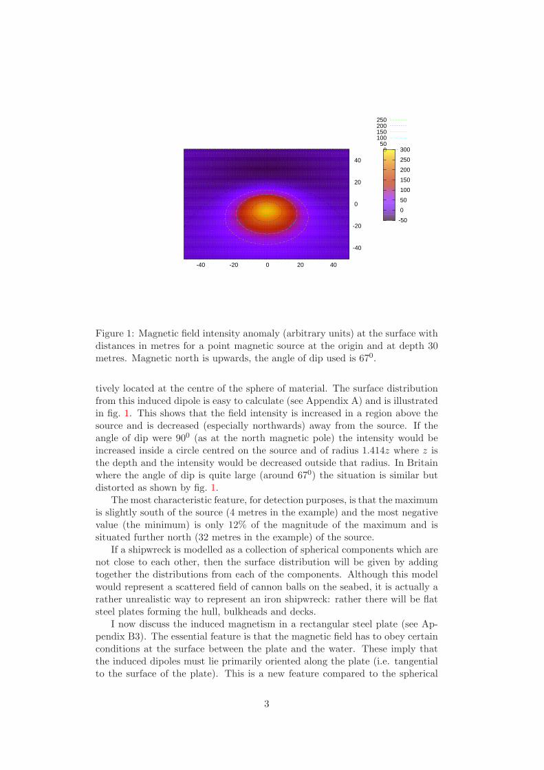
Figure 1: Magnetic field intensity anomaly (arbitrary units) at the surface withdistances in metres for a point magnetic source at the origin and at depth 30metres. Magnetic north is upwards, the angle of dip used is 670.

tively located at the centre of the sphere of material. The surface distributionfrom this induced dipole is easy to calculate (see Appendix A) and is illustratedin fig. 1. This shows that the field intensity is increased in a region above thesource and is decreased (especially northwards) away from the source. If theangle of dip were 900 (as at the north magnetic pole) the intensity would beincreased inside a circle centred on the source and of radius 1.414z where z isthe depth and the intensity would be decreased outside that radius. In Britainwhere the angle of dip is quite large (around 670) the situation is similar butdistorted as shown by fig. 1.

The most characteristic feature, for detection purposes, is that the maximumis slightly south of the source (4 metres in the example) and the most negativevalue (the minimum) is only 12% of the magnitude of the maximum and issituated further north (32 metres in the example) of the source.

If a shipwreck is modelled as a collection of spherical components which arenot close to each other, then the surface distribution will be given by addingtogether the distributions from each of the components. Although this modelwould represent a scattered field of cannon balls on the seabed, it is actually arather unrealistic way to represent an iron shipwreck: rather there will be flatsteel plates forming the hull, bulkheads and decks.

I now discuss the induced magnetism in a rectangular steel plate (see Ap-pendix B3). The essential feature is that the magnetic field has to obey certainconditions at the surface between the plate and the water. These imply thatthe induced dipoles must lie primarily oriented along the plate (i.e. tangentialto the surface of the plate). This is a new feature compared to the spherical

3

situation: the induced dipoles will not necessarily be directed along the earth’smagnetic field.

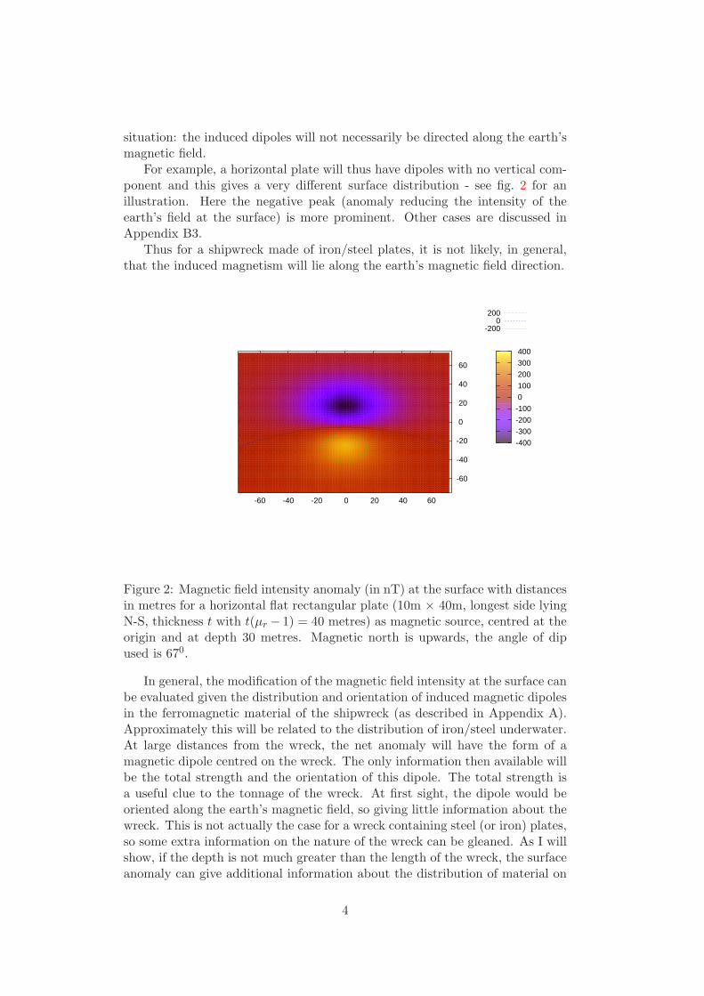
For example, a horizontal plate will thus have dipoles with no vertical com-ponent and this gives a very different surface distribution - see fig. 2 for anillustration. Here the negative peak (anomaly reducing the intensity of theearth’s field at the surface) is more prominent. Other cases are discussed inAppendix B3.

Thus for a shipwreck made of iron/steel plates, it is not likely, in general,that the induced magnetism will lie along the earth’s magnetic field direction.

-60 -40 -20 0 20 40 60

-60

-40

-20

0

20

40

60

200 0

-200

-400

-300

-200

-100

0

100

200

300

400

Figure 2: Magnetic field intensity anomaly (in nT) at the surface with distancesin metres for a horizontal flat rectangular plate (10m × 40m, longest side lyingN-S, thickness t with t(µr − 1) = 40 metres) as magnetic source, centred at theorigin and at depth 30 metres. Magnetic north is upwards, the angle of dipused is 670.

In general, the modification of the magnetic field intensity at the surface canbe evaluated given the distribution and orientation of induced magnetic dipolesin the ferromagnetic material of the shipwreck (as described in Appendix A).Approximately this will be related to the distribution of iron/steel underwater.At large distances from the wreck, the net anomaly will have the form of amagnetic dipole centred on the wreck. The only information then available willbe the total strength and the orientation of this dipole. The total strength isa useful clue to the tonnage of the wreck. At first sight, the dipole would beoriented along the earth’s magnetic field, so giving little information about thewreck. This is not actually the case for a wreck containing steel (or iron) plates,so some extra information on the nature of the wreck can be gleaned. As I willshow, if the depth is not much greater than the length of the wreck, the surfaceanomaly can give additional information about the distribution of material on

4

the seabed.Given an extended source (big ship, etc) then one solves for the induced

magnetism combining the contributions from all the iron/steel in the wreck.This can be evaluated by computer, in principle, if one knows that distribu-tion: see Appendix B4. However, if the wreck has collapsed, turned over whilesinking, been partly demolished by explosives, been salvaged, been moved bywave motion,... one will not have any accurate model of the distribution offerromagnetic material.

In practice one will need to make a simplifying model of the wreck: a flatrectangular plate, a cylinder, a shoe box, a rectangular cross-section tube,....

Some idea of the distribution of material on the seabed can be obtained ingeneral, as described in Appendix C, provided sufficiently precise surface dataare available. This is discussed later. If one makes a stronger assumption, thatall the ferromagnetic material lies at the same depth and is all magnetised inthe same direction, then it is possible to extract the material distribution onthe seabed from the surface measurement without constructing a model. Thisis discussed in Appendix C1. One always can try this approach but if regionson the seabed come out with a negative amount of material, this shows thatthe assumption was not valid. This approach is related to the method knownas ‘return to pole’ which is described in Appendix C2.

4 Permanent magnetisation effects

What is quite well established is that a ship, a few years after construction,that voyages primarily in the northern hemisphere, will have a semi-permanentmagnetisation in the vertical (downward) direction. This semi-permanent mag-netism arises from stresses in the steel of the vessel caused by wave motion,engine vibration, gunfire, heat, cargo loading, etc. It can change over a periodof a year or so. Ship’s compasses are corrected for semi-permanent and inducedmagnetism and this is a source of much expertise. Also detection of submarinesby their magnetic signature is well studied.

For example, submarines are regularly ‘depermed’ - have their permanentmagnetisation removed - by using a strong oscillating magnetic field that de-creases in strength. This reduces their magnetic ‘presence’ so they cannot beas easily detected by magnetometers. During World War II, a method of coun-teracting the magnetic ‘presence’ of a ship needed to be developed - to avoidsetting off magnetic mines. This involved a permanent electric current encir-cling the ship close to the waterline which produced a vertical magnetic fieldwhich cancelled out the semi-permanent magnetisation (and also the verticalcomponent of the induced magnetisation to some extent). This was known as‘degaussing’. Later on, deperming was also used.

A coda to this is that when magnetic mines were made more sensitive, thedegaussing currents were switched to maximise the ship’s magnetic signal -causing the mines to explode some distance away from the ship.

The magnetisation from construction (heating/cooling and hammering canboth give rise to a permanent magnetisation) is not easy to predict. What

5

emerges from the reports on magnetic effects in real ships (and submarines) isthat the vertical semi-permanent magnetic effect is usually the dominant oneafter a few years at sea. What is quite unclear to me is what happens after aship sinks. It no longer moves around and is not subject to vibration or waveslamming (if sufficiently deep). So one possibility is that the pre-sinking semi-permanent magnetisation remains. Another possibility is that it decays slowlyand what remains is the induced magnetisation caused by the earth’s magneticfield direction at the wrecksite which is what we have been discussing above.

High tensile steel would be expected to retain permanent magnetism forlonger than mild steel or iron. I can find no reliable quantitative data on thisfor steel plates used in ship building. One way to explore further is too look atknown wrecksites and see how the surface magnetic intensity can be understood.

Another complication is that for an old wreck, the direction of the earth’sfield will have changed during its period on the seabed. In the Liverpool area,magnetic north was -210 from true north in 1877 and is now (2011) much closer(-20) to true north.

This discussion of semi-permanent magnetism in ships shows that even moreuncertainty is present in trying to predict the magnetic presence of a shipwreck.The semi-permanent magnetism can be represented by a dipole distribution,just like the induced magnetism. If one instead takes the approach that thewreck is a magnetic dipole source of unknown strength, direction and distribu-tion, then it is still possible to analyse this from data on the surface anomaly.

5 Fitting surface data

Given an accurate set of data (position of measurement and value of magneticintensity shift), it should be possible to deduce something about the distri-bution of magnetic material on the seabed. The general case is discussed inAppendix C. If the surface data are sufficiently precise and extensive, it will bepossible to interpolate them accurately and hence make a 2-dimensional Fouriertransform of them. This allows in general, as discussed in Appendix C, to eval-uate quantities of interest which may help to deduce the nature of the wreck.One example considered in Appendix C is the surface anomalous magnetic en-ergy distribution. This is less sensitive (than the original data on the magneticfield anomaly) to the orientation of the dipoles induced in the shipwreck. Thesurface distribution of this quantity thus tracks the underlying distribution ofmaterial more closely - allowing the orientation of the shipwreck to be inferred,for example.

As discussed above, if the only magnetic contribution is an induced magneticdipole distribution (or a semi-permanent magnetism) in a known direction, thenone can extract the distribution at the seabed directly if one assumes that allmaterial is at the same depth. See Appendix C1.

To go beyond this case, one needs to model the distribution (and direction)of the magnetic source and then fit the parameters of the model to the datataken at the surface. By fitting, I mean minimising the χ2 which is the sum ofthe square of (data − model)/error. This will require models of the shipwreck

6

-60 -40 -20 0 20 40 60

-60

-40

-20

0

20

40

60

200 100

0 -100

-200-150-100-50 0 50 100 150 200 250 300

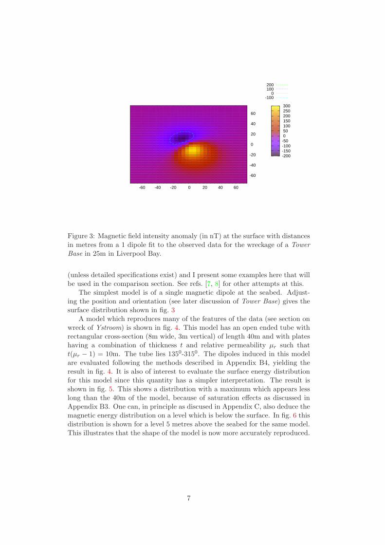
Figure 3: Magnetic field intensity anomaly (in nT) at the surface with distancesin metres from a 1 dipole fit to the observed data for the wreckage of a Tower

Base in 25m in Liverpool Bay.

(unless detailed specifications exist) and I present some examples here that willbe used in the comparison section. See refs. [7, 8] for other attempts at this.

The simplest model is of a single magnetic dipole at the seabed. Adjust-ing the position and orientation (see later discussion of Tower Base) gives thesurface distribution shown in fig. 3

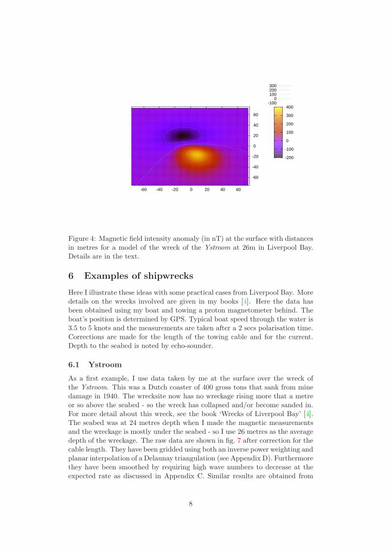
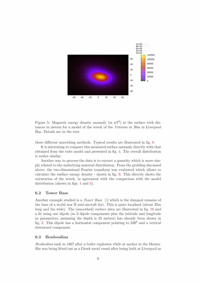
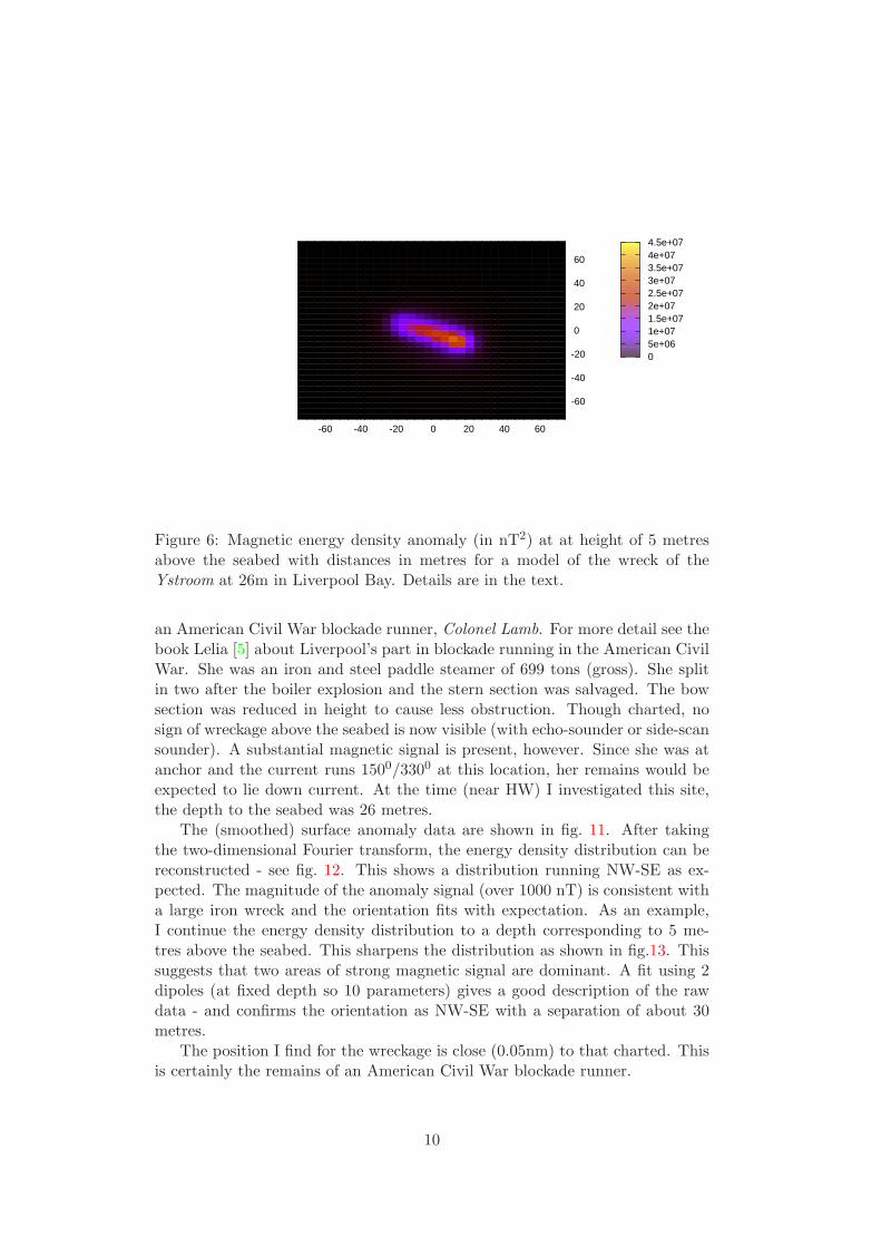
A model which reproduces many of the features of the data (see section onwreck of Ystroom) is shown in fig. 4. This model has an open ended tube withrectangular cross-section (8m wide, 3m vertical) of length 40m and with plateshaving a combination of thickness t and relative permeability µr such thatt(µr − 1) = 10m. The tube lies 1350-3150. The dipoles induced in this modelare evaluated following the methods described in Appendix B4, yielding theresult in fig. 4. It is also of interest to evaluate the surface energy distributionfor this model since this quantity has a simpler interpretation. The result isshown in fig. 5. This shows a distribution with a maximum which appears lesslong than the 40m of the model, because of saturation effects as discussed inAppendix B3. One can, in principle as discused in Appendix C, also deduce themagnetic energy distribution on a level which is below the surface. In fig. 6 thisdistribution is shown for a level 5 metres above the seabed for the same model.This illustrates that the shape of the model is now more accurately reproduced.

7

-60 -40 -20 0 20 40 60

-60

-40

-20

0

20

40

60

300 200 100

0 -100

-200

-100

0

100

200

300

400

Figure 4: Magnetic field intensity anomaly (in nT) at the surface with distancesin metres for a model of the wreck of the Ystroom at 26m in Liverpool Bay.Details are in the text.

6 Examples of shipwrecks

Here I illustrate these ideas with some practical cases from Liverpool Bay. Moredetails on the wrecks involved are given in my books [4]. Here the data hasbeen obtained using my boat and towing a proton magnetometer behind. Theboat’s position is determined by GPS. Typical boat speed through the water is3.5 to 5 knots and the measurements are taken after a 2 secs polarisation time.Corrections are made for the length of the towing cable and for the current.Depth to the seabed is noted by echo-sounder.

6.1 Ystroom

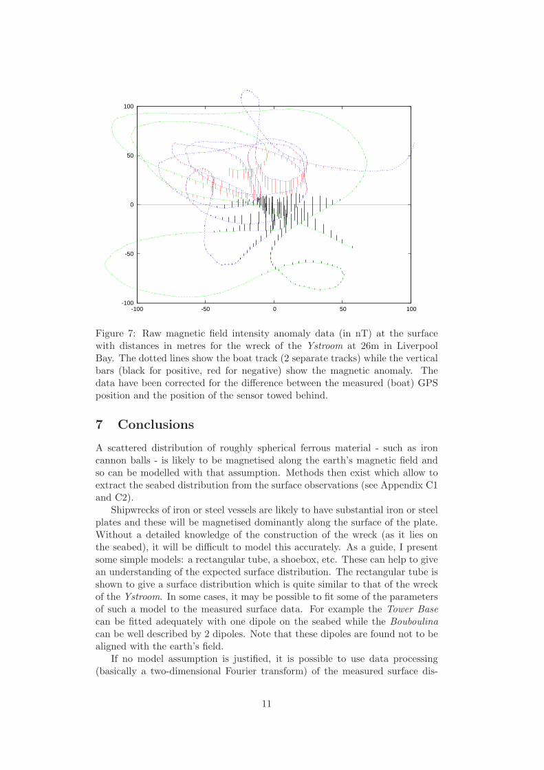
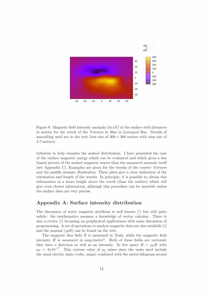
As a first example, I use data taken by me at the surface over the wreck ofthe Ystroom. This was a Dutch coaster of 400 gross tons that sank from minedamage in 1940. The wrecksite now has no wreckage rising more that a metreor so above the seabed - so the wreck has collapsed and/or become sanded in.For more detail about this wreck, see the book ‘Wrecks of Liverpool Bay’ [4].The seabed was at 24 metres depth when I made the magnetic measurementsand the wreckage is mostly under the seabed - so I use 26 metres as the averagedepth of the wreckage. The raw data are shown in fig. 7 after correction for thecable length. They have been gridded using both an inverse power weighting andplanar interpolation of a Delaunay triangulation (see Appendix D). Furthermorethey have been smoothed by requiring high wave numbers to decrease at theexpected rate as discussed in Appendix C. Similar results are obtained from

8

-60 -40 -20 0 20 40 60

-60

-40

-20

0

20

40

60

1e+05 8e+04 6e+04 4e+04 2e+04

0

20000

40000

60000

80000

100000

120000

Figure 5: Magnetic energy density anomaly (in nT2) at the surface with dis-tances in metres for a model of the wreck of the Ystroom at 26m in LiverpoolBay. Details are in the text.

these different smoothing methods. Typical results are illustrated in fig. 8.It is interesting to compare this measured surface anomaly directly with that

obtained from the tube model and presented in fig. 4. The overall distributionis rather similar.

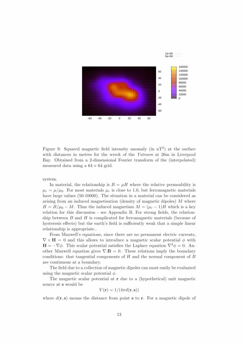
Another way to process the data is to extract a quantity which is more sim-ply related to the underlying material distribution. From the gridding discussedabove, the two-dimensional Fourier transform was evaluated which allows tocalculate the surface energy density - shown in fig. 9. This directly shows theorientation of the wreck, in agreement with the comparison with the modeldistribution (shown in figs. 4 and 5).

6.2 Tower Base

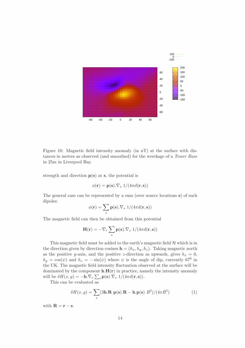
Another example studied is a Tower Base [4] which is the dumped remains ofthe base of a world war II anti-aircraft fort. This is quite localised (about 35mlong and 5m wide). The (smoothed) surface data are illustrated in fig. 10 anda fit using one dipole (so 3 dipole components plus the latitude and longitudeas parameters, assuming the depth is 25 metres) has already been shown infig. 3. This dipole has a horizontal component pointing to 3260 and a verticaldownward component.

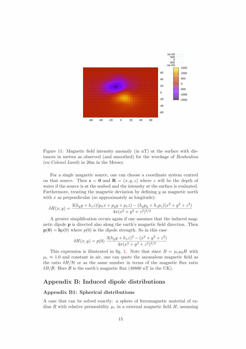
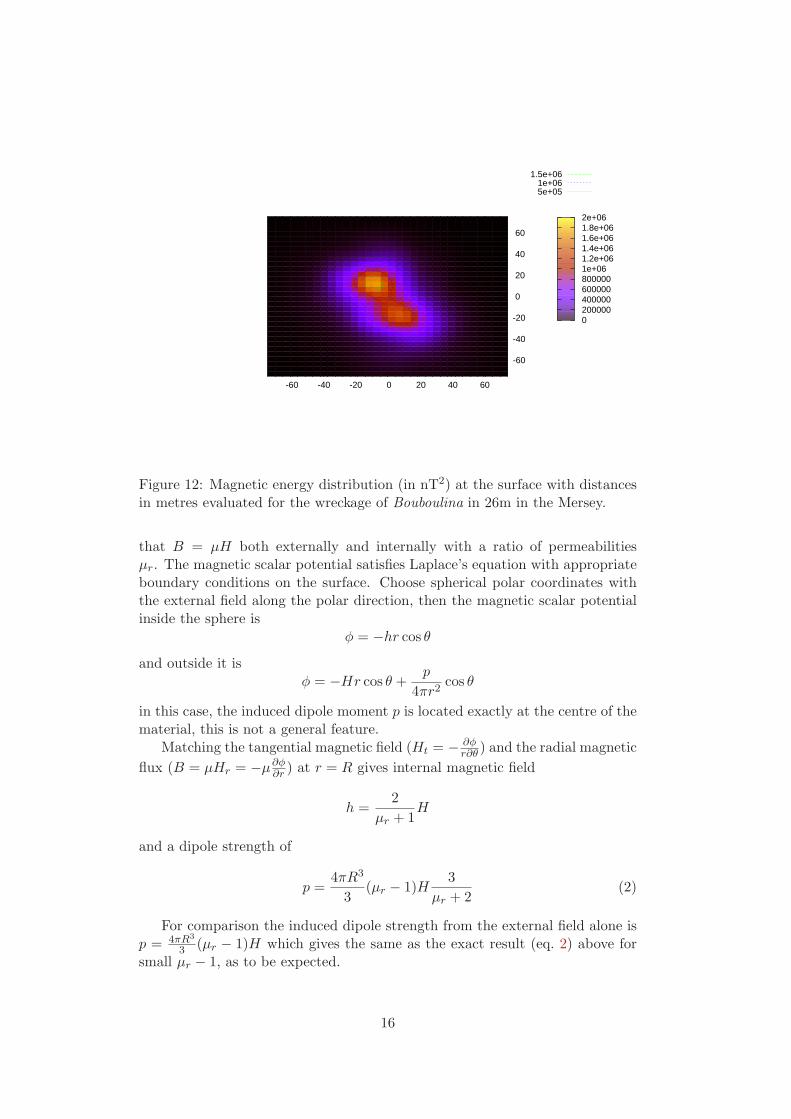
6.3 Bouboulina

Bouboulina sank in 1867 after a boiler explosion while at anchor in the Mersey.She was being fitted out as a Greek naval vessel after being built at Liverpool as

9

-60 -40 -20 0 20 40 60

-60

-40

-20

0

20

40

60

0 5e+06 1e+07 1.5e+07 2e+07 2.5e+07 3e+07 3.5e+07 4e+07 4.5e+07

Figure 6: Magnetic energy density anomaly (in nT2) at at height of 5 metresabove the seabed with distances in metres for a model of the wreck of theYstroom at 26m in Liverpool Bay. Details are in the text.

an American Civil War blockade runner, Colonel Lamb. For more detail see thebook Lelia [5] about Liverpool’s part in blockade running in the American CivilWar. She was an iron and steel paddle steamer of 699 tons (gross). She splitin two after the boiler explosion and the stern section was salvaged. The bowsection was reduced in height to cause less obstruction. Though charted, nosign of wreckage above the seabed is now visible (with echo-sounder or side-scansounder). A substantial magnetic signal is present, however. Since she was atanchor and the current runs 1500/3300 at this location, her remains would beexpected to lie down current. At the time (near HW) I investigated this site,the depth to the seabed was 26 metres.

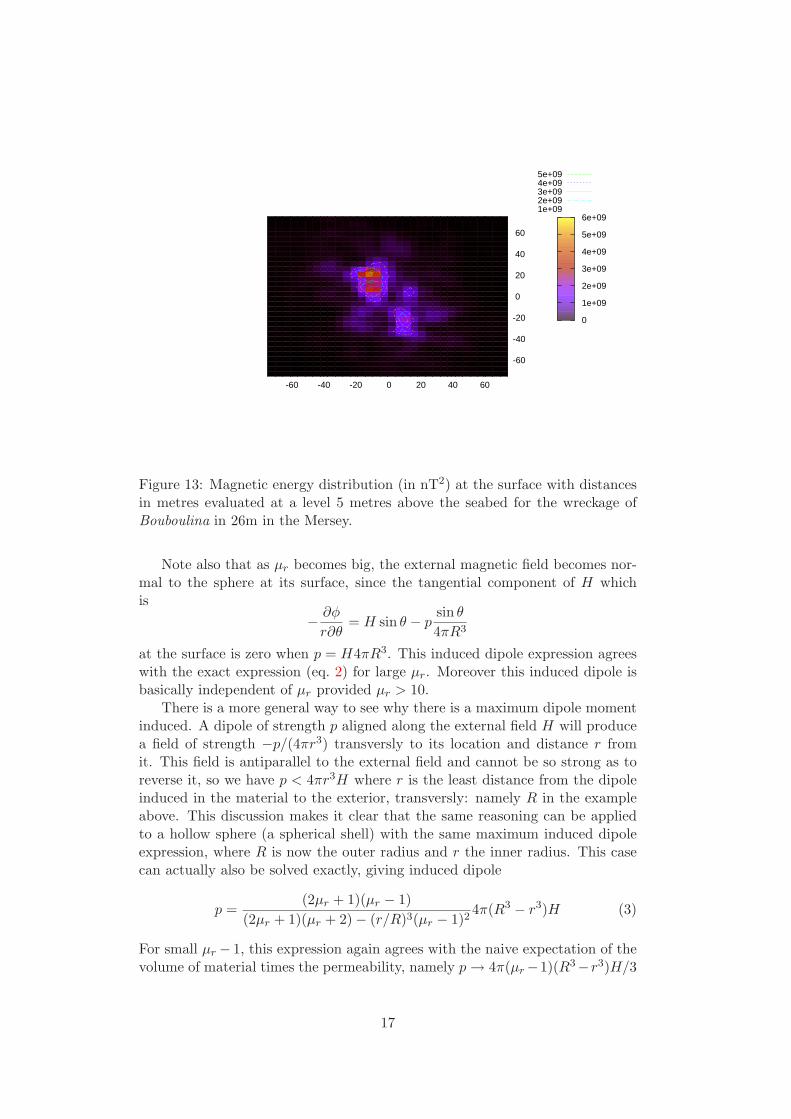
The (smoothed) surface anomaly data are shown in fig. 11. After takingthe two-dimensional Fourier transform, the energy density distribution can bereconstructed - see fig. 12. This shows a distribution running NW-SE as ex-pected. The magnitude of the anomaly signal (over 1000 nT) is consistent witha large iron wreck and the orientation fits with expectation. As an example,I continue the energy density distribution to a depth corresponding to 5 me-tres above the seabed. This sharpens the distribution as shown in fig.13. Thissuggests that two areas of strong magnetic signal are dominant. A fit using 2dipoles (at fixed depth so 10 parameters) gives a good description of the rawdata - and confirms the orientation as NW-SE with a separation of about 30metres.

The position I find for the wreckage is close (0.05nm) to that charted. Thisis certainly the remains of an American Civil War blockade runner.

10

-100

-50

0

50

100

-100 -50 0 50 100

Figure 7: Raw magnetic field intensity anomaly data (in nT) at the surfacewith distances in metres for the wreck of the Ystroom at 26m in LiverpoolBay. The dotted lines show the boat track (2 separate tracks) while the verticalbars (black for positive, red for negative) show the magnetic anomaly. Thedata have been corrected for the difference between the measured (boat) GPSposition and the position of the sensor towed behind.

7 Conclusions

A scattered distribution of roughly spherical ferrous material - such as ironcannon balls - is likely to be magnetised along the earth’s magnetic field andso can be modelled with that assumption. Methods then exist which allow toextract the seabed distribution from the surface observations (see Appendix C1and C2).

Shipwrecks of iron or steel vessels are likely to have substantial iron or steelplates and these will be magnetised dominantly along the surface of the plate.Without a detailed knowledge of the construction of the wreck (as it lies onthe seabed), it will be difficult to model this accurately. As a guide, I presentsome simple models: a rectangular tube, a shoebox, etc. These can help to givean understanding of the expected surface distribution. The rectangular tube isshown to give a surface distribution which is quite similar to that of the wreckof the Ystroom. In some cases, it may be possible to fit some of the parametersof such a model to the measured surface data. For example the Tower Base

can be fitted adequately with one dipole on the seabed while the Bouboulina

can be well described by 2 dipoles. Note that these dipoles are found not to bealigned with the earth’s field.

If no model assumption is justified, it is possible to use data processing(basically a two-dimensional Fourier transform) of the measured surface dis-

11

-60 -40 -20 0 20 40 60

-60

-40

-20

0

20

40

60

200 0

-200

-300

-200

-100

0

100

200

300

400

Figure 8: Magnetic field intensity anomaly (in nT) at the surface with distancesin metres for the wreck of the Ystroom at 26m in Liverpool Bay. Details ofsmoothing used are in the text (box size of 300 × 300 metres with step size of4.7 metres).

tribution to help visualise the seabed distribution. I have presented the caseof the surface magnetic energy which can be evaluated and which gives a lessbiased picture of the seabed magnetic source than the measured anomaly itself(see Appendix C). Examples are given for the wrecks of the coaster Ystroom

and the paddle steamer Bouboulina. These plots give a clear indication of theorientation and length of the wrecks. In principle, it is possible to obtain thisinformation at a lesser height above the wreck (than the surface) which willgive even clearer information, although this procedure can be unstable unlessthe surface data are very precise.

Appendix A: Surface intensity distribution

The discussion of static magnetic problems is well known [1] but still quitesubtle: the mathematics assumes a knowledge of vector calculus. There isalso a review [2] focussing on geophysical applications with some discussion ofprogramming. A set of operations to analyse magnetic data are also available [3]and the manual (.pdf) can be found on the web.

The magnetic flux field B is measured in Tesla, while the magnetic fieldintensity H is measured in amp/metre2. Both of these fields are vectorial:they have a direction as well as an intensity. In free space B = µ0H withµ0 = 4π10−7. This curious value of µ0 arises since the units used includethe usual electric units (volts, amps) combined with the metre-kilogram-second

12

-60 -40 -20 0 20 40 60

-60

-40

-20

0

20

40

60

1e+05 5e+04

0

20000

40000

60000

80000

100000

120000

140000

160000

Figure 9: Squared magnetic field intensity anomaly (in nT2) at the surfacewith distances in metres for the wreck of the Ystroom at 26m in LiverpoolBay. Obtained from a 2-dimensional Fourier transform of the (interpolated)measured data using a 64 × 64 grid.

system.In material, the relationship is B = µH where the relative permeability is

µr = µ/µ0. For most materials µr is close to 1.0, but ferromagnetic materialshave large values (50-10000). The situation in a material can be considered asarising from an induced magnetisation (density of magnetic dipoles) M whereH = B/µ0 −M . Thus the induced magnetism M = (µr − 1)H which is a keyrelation for this discussion - see Appendix B. For strong fields, the relation-ship between B and H is complicated for ferromagnetic materials (because ofhysteresis effects) but the earth’s field is sufficiently weak that a simple linearrelationship is appropriate..

From Maxwell’s equations, since there are no permanent electric currents,∇× H = 0 and this allows to introduce a magnetic scalar potential φ withH = −∇φ. This scalar potential satisfies the Laplace equation ∇2φ = 0. An-other Maxwell equation gives ∇.B = 0. These relations imply the boundaryconditions: that tangential components of H and the normal component of Bare continuous at a boundary.

The field due to a collection of magnetic dipoles can most easily be evaluatedusing the magnetic scalar potential φ.

The magnetic scalar potential at r due to a (hypothetical) unit magneticsource at s would be

V (r) = 1/(4πd(r, s))

where d(r, s) means the distance from point s to r. For a magnetic dipole of

13

-60 -40 -20 0 20 40 60

-60

-40

-20

0

20

40

60

100 0

-100

-150

-100

-50

0

50

100

150

200

Figure 10: Magnetic field intensity anomaly (in nT) at the surface with dis-tances in metres as observed (and smoothed) for the wreckage of a Tower Base

in 25m in Liverpool Bay.

strength and direction p(s) at s, the potential is

φ(r) = p(s).∇s 1/(4πd(r, s))

The general case can be represented by a sum (over source locations s) of suchdipoles:

φ(r) =∑

s

p(s).∇s 1/(4πd(r, s))

The magnetic field can then be obtained from this potential

H(r) = −∇r

∑s

p(s).∇s 1/(4πd(r, s))

This magnetic field must be added to the earth’s magnetic field H which is inthe direction given by direction cosines h = (hx, hy, hz). Taking magnetic northas the positive y-axis, and the positive z-direction as upwards, gives hx = 0,hy = cos(ψ) and hz = − sin(ψ) where ψ is the angle of dip, currently 670 inthe UK. The magnetic field intensity fluctuation observed at the surface will bedominated by the component h.H(r) in practice, namely the intensity anomalywill be δH(x, y) = −h.∇r

∑s p(s).∇s 1/(4πd(r, s)).

This can be evaluated as

δH(x, y) =∑

s

(3h.R p(s).R − h.p(s) R2)/(4πR5) (1)

with R = r − s.

14

-60 -40 -20 0 20 40 60

-60

-40

-20

0

20

40

60

1e+03 500

0 -500

-1e+03

-1500

-1000

-500

0

500

1000

1500

Figure 11: Magnetic field intensity anomaly (in nT) at the surface with dis-tances in metres as observed (and smoothed) for the wreckage of Bouboulina

(ex-Colonel Lamb) in 26m in the Mersey.

For a single magnetic source, one can choose a coordinate system centredon that source. Then s = 0 and R = (x, y, z) where z will be the depth ofwater if the source is at the seabed and the intensity at the surface is evaluated.Furthermore, treating the magnetic deviation by defining y as magnetic northwith x as perpendicular (so approximately as longitude):

δH(x, y) =3(hyy + hzz)(pxx+ pyy + pzz) − (hypy + hzpz)(x

2 + y2 + z2)

4π(x2 + y2 + z2)5/2

A greater simplification occurs again if one assumes that the induced mag-netic dipole p is directed also along the earth’s magnetic field direction. Thenp(0) = hp(0) where p(0) is the dipole strength. So in this case

δH(x, y) = p(0)3(hyy + hzz)

2 − (x2 + y2 + z2)

4π(x2 + y2 + z2)5/2

This expression is illustrated in fig. 1. Note that since B = µrµ0H withµr ≈ 1.0 and constant in air, one can quote the anomalous magnetic field asthe ratio δH/H or as the same number in terms of the magnetic flux ratioδB/B. Here B is the earth’s magnetic flux (48800 nT in the UK).

Appendix B: Induced dipole distributions

Appendix B1: Spherical distributions

A case that can be solved exactly: a sphere of ferromagnetic material of ra-dius R with relative permeability µr in a external magnetic field H, assuming

15

-60 -40 -20 0 20 40 60

-60

-40

-20

0

20

40

60

1.5e+06 1e+06 5e+05

0 200000 400000 600000 800000 1e+06 1.2e+06 1.4e+06 1.6e+06 1.8e+06 2e+06

Figure 12: Magnetic energy distribution (in nT2) at the surface with distancesin metres evaluated for the wreckage of Bouboulina in 26m in the Mersey.

that B = µH both externally and internally with a ratio of permeabilitiesµr. The magnetic scalar potential satisfies Laplace’s equation with appropriateboundary conditions on the surface. Choose spherical polar coordinates withthe external field along the polar direction, then the magnetic scalar potentialinside the sphere is

φ = −hr cos θ

and outside it isφ = −Hr cos θ +

p

4πr2cos θ

in this case, the induced dipole moment p is located exactly at the centre of thematerial, this is not a general feature.

Matching the tangential magnetic field (Ht = − ∂φr∂θ ) and the radial magnetic

flux (B = µHr = −µ∂φ∂r ) at r = R gives internal magnetic field

h =2

µr + 1H

and a dipole strength of

p =4πR3

3(µr − 1)H

3

µr + 2(2)

For comparison the induced dipole strength from the external field alone isp = 4πR3

3 (µr − 1)H which gives the same as the exact result (eq. 2) above forsmall µr − 1, as to be expected.

16

-60 -40 -20 0 20 40 60

-60

-40

-20

0

20

40

60

5e+09 4e+09 3e+09 2e+09 1e+09

0

1e+09

2e+09

3e+09

4e+09

5e+09

6e+09

Figure 13: Magnetic energy distribution (in nT2) at the surface with distancesin metres evaluated at a level 5 metres above the seabed for the wreckage ofBouboulina in 26m in the Mersey.

Note also that as µr becomes big, the external magnetic field becomes nor-mal to the sphere at its surface, since the tangential component of H whichis

− ∂φ

r∂θ= H sin θ − p

sin θ

4πR3

at the surface is zero when p = H4πR3. This induced dipole expression agreeswith the exact expression (eq. 2) for large µr. Moreover this induced dipole isbasically independent of µr provided µr > 10.

There is a more general way to see why there is a maximum dipole momentinduced. A dipole of strength p aligned along the external field H will producea field of strength −p/(4πr3) transversly to its location and distance r fromit. This field is antiparallel to the external field and cannot be so strong as toreverse it, so we have p < 4πr3H where r is the least distance from the dipoleinduced in the material to the exterior, transversly: namely R in the exampleabove. This discussion makes it clear that the same reasoning can be appliedto a hollow sphere (a spherical shell) with the same maximum induced dipoleexpression, where R is now the outer radius and r the inner radius. This casecan actually also be solved exactly, giving induced dipole

p =(2µr + 1)(µr − 1)

(2µr + 1)(µr + 2) − (r/R)3(µr − 1)24π(R3 − r3)H (3)

For small µr − 1, this expression again agrees with the naive expectation of thevolume of material times the permeability, namely p→ 4π(µr −1)(R3−r3)H/3

17

This expression (eq. 3) also again has the property that it saturates at verylarge µr at a value 4πR3H as we argued above. However, it can be rewrittenin a form more useful for a thin shell, with (r/R)3 = 1 − 3t/R where t is thethickness of the shell (if thin).

p =(µr − 1)(2µr + 1)

3µr + 2(µr − 1)2t/R4πR2tH (4)

The criterion is now that saturation occurs when tµr >> R. For plates usedin ship-building with thickness t ≈ 0.03 metres; µr ≈ 50 → 1000; and size ofstructure R ≈ 10 metres; then the criterion is not fully satisfied: so one doesnot necessarily have full saturation.

The induced dipole, because of the spherical symmetry, appears to be lo-cated at a point, the centre of the sphere. Thus the surface magnetic anomaly isthat given by a point dipole (see Appendix A and fig. 1). One can estimate themagnitude of the surface anomaly in a typical case: taking a sphere of radius1.7 metres which has volume about 20 m3 and mass of about 160 tons at depth30 metres. For typical µr values, there is saturation and this gives an induceddipole p = 4πR3H directed antiparallel to H which produces a magnetic fieldof approximately 2p/(4πz3) at the surface where z is the depth. This givesan anomaly 0.00035H which is very small (about 17nT given the UK value ofH). Note that a spherical shell of the same outer radius but of thickness 0.05metre with µr = 800 gives 94% of the same surface anomaly with only 9% ofthe volume, and thus mass, of ferromagnetic material.

What is learnt from these cases, is that the dipole induced by the externalfield of the earth is modified by the magnetic field produced by that induceddipole itself. This can give rise to a saturation, the induced dipole does notincrease further after µr ≈ 10 in the case of a solid object. For a thin shell, thecriterion is that saturation occurs when tµr >> R and this inequality is oftennot satisfied for ship building plates.

This discussion shows that it is not the volume of ferromagnetic materialthat determines the induced dipole strength, but rather the spatial extent. Soa relatively thin shell can have a similar induced dipole to a solid sphere.

In the case of the sphere and spherical shell, the symmetry of the situa-tion ensures that the induced dipole is aligned with the external field. Thisis not generally the case, as I illustrate with a discussion of thin plates - seeAppendices B3 and B4.

Appendix B2: a cylindrical rod and tube

When a ferromagnetic object has infinite extent in one direction, the problembecomes effectively two-dimensional and thus easier to solve exactly. One ap-plication of this is to a long hollow cylinder, which will be a useful model tocompare with computer methods to be discussed later.

Consider first an infinite solid rod of radius R with relative permeability µr

and external magnetic field H perpendicular to the axis. Choose cylindricalcoordinates, then the potential inside the rod is (using known solutions of the

18

two-dimensional Laplace equation)

φ = −hr cos θ

and outside it isφ = −Hr cos θ +

p

2πrcos θ

Matching the tangential magnetic field (Ht = − ∂φr∂θ ) and the radial magnetic

flux (B = µHr = −µ∂φ∂r ) at r = R gives internal magnetic field

h =2

µr + 1H

and a dipole strength per unit length, directed antiparallel to the external fieldH

p = 2πµr − 1

µr + 1R2H (5)

For comparison the induced dipole strength from the external field alone isp = πR2(µr − 1)H which gives the same as the exact result above for smallµr − 1, as to be expected.

Again as µr becomes big (> 10), the induced dipole strength saturates andthe external magnetic field becomes normal to the cylinder at the surface. Asbefore, a general argument shows why there is a maximum dipole momentinduced. A dipole of strength p aligned along the external field H will producea field of strength −p/(2πr2) transversly to its location and distance r from it.This field is antiparallel to the external field and cannot be such as to reverseit, so p < 2πr2H where r is the least distance from the dipole induced in thematerial to the exterior, transversly: namely R in the example above.

This discussion makes it clear that the same reasoning can be applied to ahollow cylinder with the same maximum induced dipole expression, where R isnow the outer radius. For a cylindrical shell of 1 mm thick, radius 1 metre withµr = 999, one finds this maximum is already nearly attained (83%). So a thincylindrical shell can have a similar induced dipole moment to a solid cylinderof the same outer radius. This makes it clear that the volume of ferromagneticmaterial is less important than the spatial extent in regard to the maximumdipole induced.

The exact result is also known in this case (inner radius r, outer R):

p =2π(µ2

r − 1)(R2 − r2)

(µr + 1)2 − (r/R)2(µr − 1)2(6)

and again the criterion for saturation is that tµr >> R where the thicknesst = R−r. In the above numerical example tµr = 1 and R = 1 (both in metres),so there is partial saturation.

Appendix B3: flat plates

The boundary conditions at a surface between water and ferromagnetic mate-rial are that (i) tangential components of the magnetic field H are continuous

19

and (ii) normal components of the magnetic flux B = µH are continuous. Fer-romagnetic material has a very high permeability µ and this implies that theinduced magnetisation is parallel to the surface. For a thin sheet of magneticmaterial, such as the plate of a ship, the earth’s magnetic field will inducemagnetic dipoles which have an orientation that lies in the plate.

For example, since the earth’s magnetic field lies in direction pointing tomagnetic north but downward angled, then a horizontal plate will be magnetisedwith induced dipoles pointing north, while a vertical plate oriented W-E willhave induced dipoles pointing vertically downwards.

The general case is less simple since the induced dipoles will themselvesproduce a magnetic field which needs to be taken into account consistently.I present a general method for achieving this computationally below in Ap-pendix B4.

I first discuss the relatively simple case of a thin infinite flat plate of widthl and thickness t with relative permeability µr. If the external magnetic fieldH is in the plane of the plate and perpendicular to the infinite extent, one cansolve the problem analytically though not easily. The key to understanding thesituation is that the dipole density, (µr − 1)H per unit volume, induced by Hwill be oriented along the width direction and be uniform. The field on theplate at distance x from one edge caused by that induced distribution will begiven by

1

2πHt(µr − 1)(

1

x+

1

l − x)

If this field (which is directed against the external field) is too big then theinduced dipole distribution will be reduced. The largest effect will be near theedges when x < t(µr−1)/(2π). This can be modelled as an effective reduction inthe magnetised length from l to l−t(µr−1)/π. For example with t(µr−1) = 40metres, the length reduction would be approximately 13 metres which is indeedwhat one gets from the exact solution when l > 40 metres. For example, I find,from computer evaluation (with t(µr − 1) = 40 metres again, see Appendix B4for details) that a 100 metre long plate (which would naively have an induceddipole 10 times that of a 10 metre long plate) actually has an induced dipole40 times bigger (since the self consistency effects reduce the dipole for the 10mplate substantially).

This analysis shows that the largest dipole will be induced

• when the component of the earth’s magnetic field tangential to a plate isgreatest.

• and when the length of the plate in that direction is longest.

The earth’s magnetic field component vertically is 2.36 times as great as thathorizontally (north) in UK latitudes. In most shipwrecks the vertical length ofplates is relatively short, compared to the horizontal length of plates. The extralength compensates for the lower magnetic field component, this implies thathorizontal induced dipoles are likely to be at least as important, if not more so,than vertical ones.

20

Here I make an estimate of the absolute signal from a shipwreck. Considera horizontal steel flat plate on the seabed of extent 40 metres by 10 metres andthickness t = 0.05 metres (this is thicker than a typical plate, so is supposedto account for several). It has volume 20 m3 and a mass of about 160 tons.This mass is similar to that of a small coaster. The induced dipole moment isp = 20(µr − 1)HN where HN is the component of the earth’s magnetic fieldin the magnetic north direction (so H cos(ψ)). The field produced by such adipole at the surface (horizontally, pointing south) above the dipole is p/(4πz3)and the anomaly (here a reduction in intensity) will be the component of thisalong the earth’s magnetic field, so p cos(ψ)/(4πz3). This gives a ratio of theanomaly to the total earth’s field intensity of 20(µr − 1) cos2(ψ)/(4πz3) whichgives, setting depth z = 30 metres and µr = 800, a ratio of 0.007. This issimilar to what I expect from experience of actual shipwrecks, namely a signalof around 300nT in a total of 49000nT, giving an observed ratio of 0.006.

A computer evaluation of this case (actually with (µr −1)t = 40 metres, seeAppendix B4) gives a peak (actually a trough) anomaly of -372nT if the platelies N/S and -136nT if the plate lies E/W. The largest signal, here a reduction,is not actually directly above the centre of the wreck but displaced to the north.The smaller signal for a plate lying E/W comes because the self-consistency ismore stringent in that case (the end effects are more serious if the length in theappropriate direction is only 10 metres not 40 metres as discussed above). Seefig. 2 for an illustration of the surface distribution for the N/S case.

For a vertical plate of the same size and thickness (lying with centre atdepth 30 metres, so half under the seabed), the peak anomaly is now positiveat 763nT if the plate is N/S and 599nT if it is E/W. These signals are largersince the earth’s field has a relatively larger vertical component (if the angle ofdip is 670).

Even though the earth’s magnetic field lies in a (magnetic) north - verticalplane, induced dipoles with a E/W orientation can occur in general. For in-stance a similar vertical plate lying NE/SW has a net induced dipole in direction(0.48, 0.48,−0.74) so the horizontal component is directed along the directionof the plate - as it must be.

Appendix B4: Self consistent treatment of flat plates

To determine the magnetic anomaly produced by ferromagnetic material, onealso has to take into account, consistently, the additional magnetic inductioncaused by the field produced by the induced dipoles themselves. This is com-putationally feasible, if one knows the exact location and permeability of allmagnetic material. Here I follow a method recommended for use with ships [6].

A thin plate of ferromagnetic material (thin means that the thickness issmall compared to other dimensions involved) can be treated relatively easilyas a thin shell.

Treating the ferromagnetic shell as a series of elements with surfaces Si (heretaken as flat for simplicity of presentation) labelled i = 1, . . . n, one wishes todetermine the magnetic dipoles pi induced on each element by the externalfield H. Here the induced dipoles will be treated as located at the centre of

21

each surface element. Since only the tangential component Ht of the externalfield contributes, integrating over the surface of the element i gives the induceddipole:

pi = k

∫Si

dSi (Ht −∇tφi) (7)

where k = (µ/µ0−1)t represents the thickness of the material t and the relativepermeability µr = µ/µ0. The second term on the right hand side representsthe surface component of the magnetic field created by the induced dipolesthemselves. This is the term that I discussed qualitatively in the approximatediscussion above in Appendix B3.

Now φi is the magnetic static potential on the surface element Si from allthe induced dipoles (here treated as pointlike). So

φi =

n∑j=1

pj. ∇Gij (8)

Here Gij is the Greens function (1/(4π|ri − rj |)) from the source at thecentre of element j to a coordinate in element i. Using Gauss’ theorem on thesurface of element i, one can re-express the second term in eq. 7, since

∫Si

dSi n.∇tφi =

∫idli.n φi

where dli is a length element of the closed boundary curve encircling Si andis oriented normal (and outwards) to the curve but tangential to Si. For arectangular surface element, the component in the direction (n) of the lengthof a side will be given by the difference of the integrals along the two sides normalto it. It is convenient to describe the dipole moment pi of each element i byits components in the two orthogonal directions of the sides (for a rectangularelement).

In this formulation, the unknowns are the 2n induced moments pi (whichare tangential to the surface elements so have only two components each). Thenone can solve for these induced dipoles pi by inverting a 2n × 2n matrix andhence determine the anomalous magnetic field (−∇φ) anywhere from them.

I have written computer programs to evaluate these dipoles. As a check onecan compare with known cases (such as a cylindrical shell) and one can vary thenumber of elements used and check for convergence of the result as the numberis increased. The codes run almost instantly with hundreds of elements.

The result from one example is shown for the surface magnetic anomaly infig. 4 and for the surface energy anomaly in fig. 5. This example is a rectangularcross-section tube (8m wide, 3m vertical, 40m long) with open ends and lyinghorizontally with orientation NW-SE. The thickness t satisfies t(µr −1) = 10m.This was evaluated using a model with many small rectangular elements asdescribed above (96 elements are sufficient).

22

Appendix C: analysing the surface field

Here I first consider the general case: assuming only that the magnetic dipolesources are located in a limited area near the seabed - so away from the surface.In general, there might also be some geophysical source of magnetism in therocks under the seabed - this is called a ‘magnetic anomaly’ on the sea charts.Here I assume that the magnetic dipoles are in a localised region - as would bethe case for a shipwreck.

The anomalous magnetic field H at the surface then can be derived from apotential φ (where H = −∇φ) which satisfies the Laplace equation (∇.∇φ = 0).The observed intensity shift δH is given by h.H where h is the (known) directionof the earth’s magnetic field.

From the property that ∇.H = 0, it follows, from the Gauss theorem, that

∫dxdy Hz = 0

Also, since H can be derived from a potential, it follows that

∫dx Hx =

∫dy Hy = 0

Thus the observed anomaly satisfies

∫dxdy δH = 0

This is a useful cross-check on any data taken.At large distance (r) from the shipwreck, the anomalous magnetic field

(given by eq. 1) will decrease as 1/r3 or faster. This can also be used to cross-check data.

A very useful way to analyse data is with the two-dimensional Fourier trans-form:

δH(u, v, z) =

∫dxdy e−iux−ivyδH(x, y, z)

Here u and v will be referred to as wave-numbers. The inverse of thistransform is given by:

δH(x, y, z) =1

4π2

∫dudv eiux+ivyδH(u, v, z)

In terms of the potential and its Fourier transform φ(u, v, z), we have

φ(x, y, z) =1

4π2

∫dudveiux+ivyφ(u, v, z)

and the Laplace equation constraint implies that

∂2φ(u, v, z)

∂z2= (u2 + v2)φ(u, v, z) (9)

23

Defining k2 = u2 + v2, then ∂φ(u, v, z)/∂z = −kφ(u, v, z) since φ mustdecrease at large values of z. This enables evaluation of the gradient of φ andhence the magnetic field associated with it:

H(u, v, z) = (−iu, −iv, k)φ(u, v, z)

Thus the potential can be extracted from the observed magnetic field anomalywhich is measured at the surface (z is the height of the surface above theseabed):

φ(u, v, z) =δH(u, v, z)

−iuhx − ivhy + khz

Note that when u = 0 and v = 0, then k = 0 and hence the division isill-defined. This case corresponds to the sum of δH over all space which mustbe zero as discussed above. So there is a 0/0 situation: the average value ofφ(x, y, z) over x and y is not determined. This is resolved by the fact that anoverall constant change to φ(x, y, z) is not physically important - only differencesof potential values are significant. Moreover, in practice, one may not need toextract the potential itself, but quantities such as magnetic field componentsderived from differences of it.

In order to illustrate the significance of the two-dimensional Fourier trans-form, I present the transform of the general case given in eq. 1 in Appendix A.Since the transform of (x2 + y2 + z2)−1/2 is 2π exp(−kz)/k where k2 = u2 + v2,one can evaluate

δH(u, v, z) =∑

s

h.K ps.K e−iusx−ivsye−k(z−sz)/(2k)

where the wave-number vector K = (−iu,−iv, k) and the sum is over dipolesof strength and direction ps located at (sx, sy, sz)

The most noticeable feature of this expression is the factor exp(−kz) whichcan be deduced on general grounds from the Laplace equation as shown in eq. 9.This factor controls the rate at which the Fourier transform decreases for largewave-number. Large wave-number is related to finer structure: so this can beseen as the quantitative expression of the fact that the surface distribution willbe smoother, the deeper is the wreck. This can be used to smooth data - byrequiring that the wave-number distribution falls off in magnitude as k exp(−kz)at large k.

One can also estimate the range of important wave-numbers since k exp(−kz)is maximum at k ≈ 1/z. If a total spatial size L × L with grid step intervals × s is used to process the data, the range of sizes of wave-number will befrom 2π/L to π/s. Ideally the minimum non-zero wave number (2π/L) shouldbe several times smaller than the typically important wave-number (1/z). Thisimplies L > 2πz. So for a depth z of 25 metres the box size used should be oflinear size greater than 160 metres.

As well as the potential (and derived quantities) at the surface (height zabove the wreckage), one can evaluate the potential at a lesser height (z0 < z

24

and z0 greater than the vertical coordinate of any part of the wreckage itself)above the wreck since

φ(u, v, z0) = ek(z−z0)φ(u, v, z)

Since k2 = u2+v2, this will enhance contributions with larger u and v whichcorrespond to more detailed structures in x and y. Thus, at least in principle,one can continue the surface data down to a small height z0, such that z0 is aboveevery part of the wreck, which will show up the detailed spatial structure moreclearly. This, of course, relies on having sufficient precision in the data taken atthe surface. Only in that case will the high wave-number components reproducethe required rate of drop off (as exp(−kz)). As an estimate, if the data areavailable with a step size of s metres, then the enhancement exp k(z − z0) willbe expπ(z − z0)/s for the largest wave-numbers. If z − z0 > s, this largeenhancement factor will multiply the very small contribution from such largewave-numbers, but the numerical procedure of obtaining the Fourier transformfor such large wave-numbers may introduce errors that de-stabilize the analysis.Hence possible instabilities can arise in continuing to lower depths by an amountgreater than the spatial resolution s.

Returning to the discussion of an appropriate combination to evaluate, oncethe potential has been evaluated, one suitable combination is H.H, which isproportional to the total anomalous magnetic field energy at the surface. Thisquantity is less sensitive to the orientation of the magnetic dipoles at the seabedthan the observed anomaly itself (δH = h.H). Indeed, from a dipole p atrelative position R,

H.H = p2 3 cos2 θ + 1

16π2R6

where θ is the angle between the directions of p and R. Thus the signal isalways positive and varies by a factor of, at most, 4 for any θ at fixed distanceR. This makes the surface signal easier to interpret, compared to δH which canhave sign changes, etc. Furthermore, this quantity will show quite a localisedsurface distribution: for instance, a point source at depth z will spread out onthe surface so that the peak lies above the point source and the signal drops to50% within a circle of radius z/2 (for the case of a vertical dipole).

This can be illustrated with the rectangular tube model of a shipwreckintroduced in Appendix B4, yielding the result in fig. 4 for the surface anomaly.For the same model, the surface energy distribution is shown in fig. 5. Thisis closer to the underlying material distribution but shows a distribution witha maximum which appears less long than the 40m of the model, because ofsaturation effects as discussed in Appendix B3. One can, in principle as discusedabove, also deduce the magnetic energy distribution on a level which is belowthe surface. In fig. 6 this distribution is shown for a level 5 metres above theseabed for the same model. This illustrates that the shape of the model is nowmore accurately reproduced.

As a practical example, I show the distribution of H.H on the surface forthe wreck of the Ystroom in fig. 9. This shows a distribution lying NW-SE,

25

in agreement with the result of comparing models with the observed surfaceanomaly distribution.

Another combination,√

H.H, has an even smaller dependence on the ori-entation of seabed dipoles (a factor of 2 at maximum) and would be a possiblequantity to present. For a dipole at the seabed, the combination H.H has amore peaked spatial distribution at the surface, and this is why I favour it.

Using the above formalism to evaluate H.H at a lesser height (z0) abovethe seabed, gives rather noisy and unstable results (unless very accurate dataexist or unless the data are processed taking account of the expected decreasewith wave number) if evaluated more than a few metres below the surface, asexpected from the discussion above.

Appendix C1: deducing the bottom distribution

Here I consider a simple model: all the ferro-magnetic material lies at the samedepth below the surface (z) and it is all magnetized along the same directiona. Then p(s) = ap(s) where p(s) is the dipole strength.

This assumption could be appropriate to a wreck consisting of a scatteredcollection of iron cannon balls, for example. They will then all be magnetisedalong the earth’s magnetic field direction which is the special case that thedirection a is that of the earth’s magnetic field itself (h).

From Appendix A the observed deviation in magnetic field intensity will begiven by eq. 1

δH(x, y) =∑

s

(3h.R p(s).R − h.p(s) R2)/(4πR5)

where one introduces a magnetic dipole density ρ(sx, sy) to describe the seabeddistribution and makes use of the fixed direction of the induced dipoles. So

δH(x, y) =

∫dsxdsy (3h.R a.R − h.a R2)ρ(s)/(4πR5)

This expression has the form of a convolution

δH(x, y) =

∫dsxdsy G(x− sx, y − sy)ρ(sx, sy)

where G is a known function since z has been fixed at the depth below thesurface and h and a are both known. Our aim is to measure δH(x, y) andthence deduce ρ(sx, sy). This can be achieved by taking the 2-dimensionalFourier transform of the expression, using

G(u, v) =

∫dxdy e−iux−ivyG(x, y) = h.K a.K e−kz/(2k)

δH(u, v) =

∫dxdy e−iux−ivyδH(x, y)

Then ρ(u, v) = δH(u, v)/G(u, v) and so one can reconstruct

26

ρ(sx, sy) =1

4π2

∫dudv eiusx+ivsyρ(u, v)

However, as noted in the previous section, the correction 1/G(u, v) will bevery large for large wave number (k) because of the exponential factor exp(kz).This will render the approach unstable unless very precise data are available togive an accurate Fourier transform of δH(x, y).

Appendix C2: Return to pole derivation

At the magnetic north pole, where the magnetic field is vertical, the magneticintensity pattern on the surface above a magnetic item can be interpreted moreeasily. An isolated magnetised region will show an enhancement directly aboveit and a decrease all around. So, roughly, the area of increased magnetic inten-sity will correspond to the presence of iron below. This makes interpretation ofthe surface anomaly easier.

However, Britain is not at the north magnetic pole. With some key assump-tions, it is possible to process data so that they are in the form they would takeif they were measured at the north pole. This is known as ‘Return to pole’.

As discussed in Appendix A, the magnetic field intensity change observedat the surface will be given in terms of the magnetic scalar potential V from a(hypothetical) unit point magnetic source at s by

δH(x, y) = −h.∇r

∑s

p(s).∇s V (R)

with R = r − s where r = (x, y, z) is the coordinate of observation and s is thelocation of the magnetic dipole source (of strength and direction given by p(s).

The key assumption is that the magnetic dipoles induced are all alignedalong the earth’s magnetic field direction given by h. Again (as in Appendix C1)this assumption is most appropriate for a scattered collection of wreckage -rather than a ship with iron plates. So p(s) = hp(s) where p(s) is the dipolestrength at s and h is independent of s. One may include this factor of p(s)within the sum over sources defining a scalar potential Φ (note not the same asφ introduced in the introduction to Appendix C): Φ =

∑s p(s)V (R)

Now consider the Fourier transform (in the two horizontal spatial coordi-nates x and y of r). Here z is the vertical coordinate of r.

Φ(x, y, z) =1

4π2

∫dudv eiux+ivyΦ(u, v, z)

Since the potential satisfies Laplace’s equation ∇.∇Φ = 0. This implies that

(u2 + v2)Φ(u, v) =∂2Φ(u, v)

∂z2= k2Φ(u, v)

This allows the gradients to be evaluated, giving the magnetic field intensityanomaly

δH(x, y, z) =1

4π2

∑s

∫dudv ((−iu,−iv, k).h)2p(s)eiux+ivyΦ(u, v, z)

27

In contrast the field at the surface when the earth’s magnetic field is vertical(at the pole) is given by h = (0, 0, 1). Hence

δHpole(x, y, z) =1

4π2

∑s

∫dudv k2p(s)eiux+ivyΦ(u, v, z)

Within our assumptions, these two expressions are related by a factor ofk2/(−ihxu − ihyv + hzk)

2 where k2 = u2 + v2. This factor is independent ofthe source s and so one does not need to know the distribution of magneticmaterial in order to make the correction.

Thus the u, v Fourier transform of the measured intensity δH(x, y, z) canbe corrected by this factor where h is known. For simplicity, neglecting themagnetic deviation and choosing y as latitude, hx = 0, hy = cos(ψ), hz =− sin(ψ) where ψ is the angle of dip.

Appendix D: Interpolating point data

Assume one has logged data (such as the magnetic intensity at the surface) ata set of locations. Data values are v(xi, yi) with i = 1, . . . n representing then values logged at locations (xi, yi). One needs to interpolate these values forseveral purposes: to make a Fourier transform, to draw a smooth surface on aplot, etc.

One straightforward way to do this is to make a weighted average of thedata.

v(x, y) =1

W

n∑i=1

v(xi, yi)w(x− xi, y − yi)

with W =∑n

i=1w(x− xi, y − yi).A sensible weight to use is one that emphasises close values preferentially:

w(x− xi, y − yi) =1

((x− xi)2 + (y − yi)2)p

Choosing p = 1 corresponds to using an inverse square distance as weight.Choosing very large p corresponds to using the nearest data point. A reasonablecompromise occurs using an inverse power such as p = 2.

Note that this approach is appropriate for interpolating data but it willnot reproduce the property that a magnetic field intensity should drop off witha known power (the inverse cube) at large distances unless this condition isexplicitly imposed.

A more sophisticated way to interpolate data is to introduce a triangularnetwork in x, y and use planar interpolation (in x, y, v) in each such triangle.The usual choice of triangles is that corresponding to the Delaunay triangulation(this has no other vertex points in the circumcircle of any triangle). To set upsuch a triangulation, one must avoid repeated vertices and sets of three or morevertices lying on a line. It can also be helpful to add a few vertices near theboundary (with v value zero) if there are not measurements in that region.

28

References

[1] J. D. Jackson, Classical Electrodynamics, Wiley 1975.

[2] R. J. Blakely, Potential Theory in Gravity and Magnetic Applications, CUP1996.

[3] MagPick software package.(www.geometrics.com/geometrics-products/geometrics-magnetometers/download-magnetomet

[4] C. Michael, Wrecks of Liverpool Bay and Wrecks of Liver-

pool Bay Volume II, Liverpool Marine Press, 1994 and 2008. (www.liv.ac.uk/~cmi/books/books.html )

[5] C. Michael, Lelia, Liverpool Marine Press and Countyvise, 2004. (www.liv.ac.uk/~cmi/books/books.html )

[6] O. Chadebec, J.-L. Coulomb, V. Leconte, J.-P. Bongiraud, and G. Cauffet,Modeling of static magnetic anomaly created by iron plates, IEEE TRANS-ACTIONS ON MAGNETICS, VOL. 36, NO. 4, JULY 2000, p667

[7] C. Wang et al., The magnetic detection of sunken ships in the Madang

section of the Yangtze river, Journal of Environmental and EngineeringGeophysics (JEEG) vol 11 (2006) 123-131.

[8] N. Kinneging et al., Magnetometry in wreck removal Western Scheldt Hy-dro International, vol. 8 no. 7 (2004).

29