Magnetic cannon: The physics of the Gauss rifle

Arsene Chemin, Pauline Besserve, Aude Caussarieu, Nicolas Taberlet, and Nicolas Plihona)

Univ. Lyon, Ens de Lyon, Univ. Claude Bernard, CNRS, Laboratoire de Physique, F-69342 Lyon, France

(Received 6 July 2016; accepted 9 March 2017)

The magnetic cannon is a simple device that converts magnetic energy into kinetic energy. When a

steel ball with low initial velocity impacts a chain consisting of a magnet followed by addition

steel balls, the last ball in the chain gets ejected at a much larger velocity. The analysis of this

spectacular device involves an understanding of advanced magnetostatics, energy conversion, and

the collision of solids. In this article, the phenomena at each step of the process are modeled to

predict the final kinetic energy of the ejected ball as a function of a few parameters that can be

experimentally measured. VC 2017 American Association of Physics Teachers.

[http://dx.doi.org/10.1119/1.4979653]

I. INTRODUCTION

A. What is a magnetic cannon?

The magnetic cannon, sometimes referred to as the Gaussrifle, is a simple device that accelerates a steel ball throughconversion of magnetic energy into kinetic energy.1–4

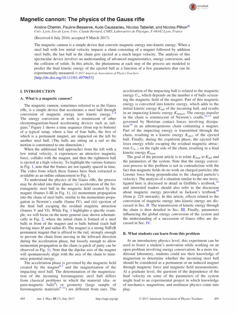
The energy conversion at work is reminiscent of otherelectromagnetism-based accelerating devices such as rail-guns.5 Figure 1 shows a time sequence (from top to bottom)of a typical setup, where a line of four balls, the first ofwhich is a permanent magnet, are impacted on the left byanother steel ball. (The balls are sitting on a rail so themotion is constrained to one dimension.)

When the additional ball approaches from the left with alow initial velocity, it experiences an attractive magneticforce, collides with the magnet, and then the rightmost ballis ejected at a high velocity. To highlight the various featuresin Fig. 1, note that the frames are not equally spaced in time.The video from which these frames have been extracted isavailable as an online enhancement to Fig. 1.

To understand the physics of the Gauss rifle, the processmay be divided into three phases: (i) acceleration of the fer-romagnetic steel ball in the magnetic field created by themagnet (frames I–III in Fig. 1), (ii) momentum propagationinto the chain of steel balls, similar to the momentum propa-gation in Newton’s cradle (frame IV), and (iii) ejection ofthe final ball escaping the residual magnetic attraction(frames V and VI). While Fig. 1 highlights a specific exam-ple, we will focus on the more general case shown schemati-cally in Fig. 2, where the initial chain is formed of n steelballs in front of the magnet and m balls behind (each ballhaving mass M and radius R). The magnet is a strong NdFeBpermanent magnet that is affixed to the rail, strongly enoughto prevent the chain from moving in the leftward directionduring the acceleration phase, but loosely enough to allowmomentum propagation in the chain (a patch of putty can beobserved in Fig. 1). Note that the dipolar axis of the magnetwill spontaneously align with the axis of the chain to mini-mize potential energy.

The acceleration phase is governed by the magnetic fieldcreated by the magnet6,7 and the magnetization of theimpacting steel ball. The determination of the magnetiza-tion of the incoming ferromagnetic steel ball differsfrom classical problems in which the material (dia- orpara-magnetic balls8) or geometry (large sample offerromagnetic materials9–11) are different from ours. The

acceleration of the impacting ball is related to the magneticenergy Un, which depends on the number n of balls screen-ing the magnetic field of the magnet. Part of this magneticenergy is converted into kinetic energy, which adds to theinitial kinetic energy Kinit of the incoming ball, and resultsin an impacting kinetic energy Kimpact. The energy transferin the chain is reminiscent of Newton’s cradle,12,13 andgoverned by Hertzian contact forces involving dissipa-tion14 in an inhomogeneous chain containing a magnet.Part of the impacting energy is transmitted through thechain, resulting in a kinetic energy Keject of the ejectedball. Finally, during the expulsion phase, the ejected ballloses energy while escaping the residual magnetic attrac-tion Um�1 on the right side of the chain, resulting in a finalkinetic energy Kfinal.

The goal of the present article is to relate Kfinal to Kinit andthe parameters of the system. Note that the energy conver-sion process in this problem is not in contradiction with thefact that magnetic fields do no work on charged particles (theLorentz force being perpendicular to the charged particle’svelocity). The analysis of a situation similar to the one inves-tigated here is discussed in detail in Griffiths’s textbook,15

and interested readers should also refer to the discussionabout magnetic energy provided in Jackson’s textbook16

(from p. 224 onwards). In this article, effects related to theconversion of magnetic energy into kinetic energy are dis-cussed in Sec. II. The transmission of kinetic energy throughthe chain is then detailed in Sec. III. Finally, parametersinfluencing the global energy conversion of the system andthe understanding of a succession of Gauss rifles are dis-cussed in Sec. IV.

B. What students can learn from this problem

At an introductory physics level, this experiment can beused to foster a student’s motivation while working on anopen problem involving energy conservation. In a more tra-ditional laboratory, students could use their knowledge ofmagnetism to determine whether the incoming steel ballshould be considered as a permanent or an induced magnetthrough magnetic force and magnetic field measurements.At a graduate level, the question of the dependence of thefinal velocity on some of the parameters of the systemmight lead to an experimental project in which knowledgeof mechanics, magnetism, and nonlinear physics come intoplay.

495 Am. J. Phys. 85 (7), July 2017 http://aapt.org/ajp VC 2017 American Association of Physics Teachers 495

II. FROM MAGNETIC ENERGY TO KINETIC

ENERGY

In this section, we investigate the conversion of magneticenergy Un into kinetic energy in the acceleration phase, aswell as the symmetric problem of the decrease of kineticenergy by Um�1 in the ejection phase. Direct measurement ofthe spatial dependence of the magnetic force exerted by themagnet on the incoming (ejected) ball and of the magneticfield is in agreement with a permanent dipole/induced dipolemodeling.

A. Force exerted by the chain on a steel ball: Apermanent/induced dipole interaction

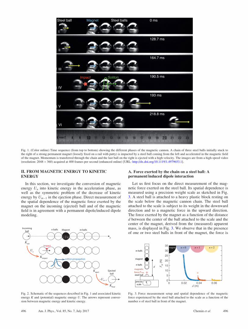
Let us first focus on the direct measurement of the mag-netic force exerted on the steel ball. Its spatial dependence ismeasured using a precision weight scale as sketched in Fig.3. A steel ball is attached to a heavy plastic block resting onthe scale below the magnetic cannon chain. The steel ballattached to the scale is subject to its weight in the downwarddirection and to a magnetic force in the upward direction.The force exerted by the magnet as a function of the distanced between the center of the ball attached to the scale and thecenter of the magnet, derived from the (measured) apparentmass, is displayed in Fig. 3. We observe that in the presenceof one or two steel balls in front of the magnet, the force is

Fig. 1. (Color online) Time sequence (from top to bottom) showing the different phases of the magnetic cannon. A chain of three steel balls initially stuck to

the right of a strong permanent magnet (loosely fixed on a rail with putty) is impacted by a steel ball coming from the left and accelerated in the magnetic field

of the magnet. Momentum is transferred through the chain and the last ball on the right is ejected with a high velocity. The images are from a high-speed video

(resolution: 2048� 360) acquired at 400 frames per second (enhanced online) [URL: http://dx.doi.org/10.1119/1.4979653.1].

Fig. 2. Schematic of the sequences described in Fig. 1 and associated kinetic

energy K and (potential) magnetic energy U. The arrows represent conver-

sion between magnetic energy and kinetic energy.

Fig. 3. Force measurement setup and spatial dependence of the magnetic

force experienced by the steel ball attached to the scale as a function of the

number n of steel ball in front of the magnet.

496 Am. J. Phys., Vol. 85, No. 7, July 2017 Chemin et al. 496

screened but is nonetheless larger than it would have beenwith a chain of non-magnetic balls, since the ferromagneticballs channel the magnetic field. A second observation, notillustrated here, is that the number of balls behind the magnethas no noticeable influence on the force exerted on the oppo-site side.

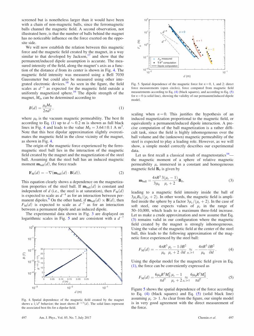
We will now establish the relation between this magneticforce and the magnetic field created by the magnet, in a waysimilar to that developed by Jackson,17 and show that thepermanent/induced dipole assumption is accurate. The mea-sured intensity of the field, along the magnet’s axis as a func-tion of the distance d from its center is shown in Fig. 4. Themagnetic field intensity was measured using a Bell 7030Gaussmeter but could also be measured using other inte-grated electronic devices.18 As seen in the figure, the fieldscales as d�3 as expected for the magnetic field outside auniformly magnetized sphere.16 The dipole strength of themagnet, M0, can be determined according to

B dð Þ ¼ l0M0

2pd3; (1)

where l0 is the vacuum magnetic permeability. The best fitaccording to Eq. (1) up to d � 0:2 m is shown as full blacklines in Fig. 4 and leads to the value M0 ¼ 3:6460:1 A m2.Note that this best dipolar approximation slightly overesti-mates the magnetic field in the close vicinity of the magnet,as shown in Fig. 4.

The origin of the magnetic force experienced by the ferro-magnetic steel ball lies in the interaction of the magneticfield created by the magnet and the magnetization of the steelball. Assuming that the steel ball has an induced magneticmoment mball dð Þ, the force reads

FM dð Þ ¼ �r mball dð Þ � B dð Þð Þ: (2)

This equation clearly shows a dependence on the magnetiza-tion properties of the steel ball. If mball dð Þ is constant andindependent of d (i.e., the steel is at saturation), then FM dð Þis expected to scale as d�4 as for an interaction between per-manent dipoles.6 On the other hand, if mball dð Þ / B dð Þ, thenFM dð Þ is expected to scale as d�7 as for an interactionbetween a permanent dipole and an induced dipole.

The experimental data shown in Fig. 3 are displayed onlogarithmic scales in Fig. 5 and are consistent with a d�7

scaling when n¼ 0. This justifies the hypothesis of aninduced magnetization proportional to the magnetic field, orequivalently a permanent/induced dipole interaction. A pre-cise computation of the ball magnetization is a rather diffi-cult task, since the field is highly inhomogeneous over theball volume and the (unknown) magnetic permeability of thesteel is expected to play a leading role. However, as we willshow, a simple model correctly describes our experimentaldata.

Let us first recall a classical result of magnetostatics16—the magnetic moment of a sphere of relative magneticpermeability lr immersed in a constant and homogeneousmagnetic field B0 is given by

mball ¼4pR3

3l0

3 lr � 1ð Þlr þ 2

B0; (3)

leading to a magnetic field intensity inside the ball of3lrB0= lr þ 2ð Þ. In other words, the magnetic field is ampli-fied inside the sphere by a factor 3lr= lr þ 2ð Þ. In the case ofsoft steel, one expects values of lr in the range of50–10,000, which leads to a maximum three-fold increase.Let us make a crude approximation and now assume that Eq.(3) remains valid in our configuration where the magneticfield created by the magnet is strongly inhomogeneous.Using the value of the magnetic field at the center of the steelball, this leads to the following approximation of the mag-netic force experienced by the steel ball:

FM dð Þ ¼ � 4pR3

l0

lr � 1

lr þ 2

@B2

@d�

lr�1� 4pR3

l0

@B2

@d: (4)

Using the dipolar model for the magnetic field given in Eq.(1), the force can be conveniently expressed as

FM dð Þ ¼ 6l0R3M20

pd7

lr � 1

lr þ 2�

lr�1

6l0R3M20

pd7: (5)

Figure 5 shows the spatial dependence of the force accordingto Eq. (4) (black squares) and Eq. (5) (solid black line)assuming lr � 1. As clear from the figure, our simple modelis in very good agreement with the direct measurement ofthe force.

Fig. 4. Spatial dependence of the magnetic field created by the magnet

shows a 1=d3 behavior; the inset shows B�1=3 dð Þ. The solid lines represent

the associated best fits for a dipolar field.

Fig. 5. Spatial dependence of the magnetic force for n¼ 0, 1, and 2: direct

force measurements (open circles), force computed from magnetic field

measurements according to Eq. (4) (black squares), and according to Eq. (5)

for n¼ 0 (a solid line), showing the validity of our permanent/induced dipole

model.

497 Am. J. Phys., Vol. 85, No. 7, July 2017 Chemin et al. 497

Establishing a theoretical expression of the magnetic fieldcreated by the magnet and channeled through one or twoballs in front of the magnet (n¼ 1, 2 in Fig. 5) is beyond thescope of the present article. However, Fig. 5 shows that theestimate of the magnetic force given in Eq. (4) is in reason-able agreement with the direct measurement.

B. Conversion of magnetic energy into kinetic energy

The available magnetic energy in the presence of n steelballs in front of the magnet are computed from the above spa-tial dependence of the magnetic force as

Ð�2 nþ1ð ÞR�1 FM xð Þ dx,

where the upper limit of the integral is the minimum approach-ing distance of the center of the incoming ball from the centerof the magnet. This magnetic energy be found either by (i)integrating the measured force profile, or (ii) integrating theforce expressed as a function of the gradient B2 according toEq. (4), which leads to Un ¼ 4pR3B2 2 nþ 1ð ÞR½ �=l0. Table Isummarizes the available magnetic energy according to thesecomputations for n¼ 0, 1, and 2. As expected from Sec. II A, avery good agreement is observed between these values, andthe available magnetic energy can be conveniently computedfrom the magnetic field measurement.

Note that a third computation of Un can also be performedby integrating Eq. (5) when n¼ 0, giving U0 ¼ l0M2

0=64pR3

¼ 9565 mJ. This higher estimate can be understood fromthe slight overestimation of the magnetic field in the vicinityof the magnet using the dipolar approximation. Since mostof the acceleration occurs very close to the magnet, this leadsto an overestimate of 25% of the available magnetic energy.However, as shown below, the expression of the force givenin Eq. (5) is useful to predict the time evolution of the speedof the impacting ball.

A partial conclusion can be drawn here for the optimiza-tion of the magnetic cannon. Acceleration in the attractionphase and deceleration in the ejection phase is controlled bythe magnetic energies Un and Um�1, which represent, respec-tively, the loss and gain of magnetic (potential) energy (andresulting in the gain and loss of kinetic energy, respectively).As Un strongly decreases with n, the maximum increase ofkinetic energy is achieved for the lowest value of n (i.e.,n¼ 0), while the minimum losses are obtained for large val-ues of m – 1. The optimization of the number m of ballsbehind the magnet depends on competing effects betweenreducing Um�1 and reducing the transfer losses within thechain during the soliton propagation. This issue will beaddressed in Sec. IV.

Let us now consider the conversion of the available mag-netic energy Un into kinetic energy. The incoming ball issubject to magnetic, friction, and drag forces. However, bothfriction and drag forces may be neglected; the magneticforce is on the order of 10 N while for M¼ 28-g balls and a

maximum velocity of the order of 3 m/s the friction force isestimated to be around 0.03 N and the viscous drag forcearound 10�4 N. Because the magnetic force stronglyincreases as the distance between the incoming ball and themagnet decreases, most of the acceleration occurs in closevicinity of the magnet. As a consequence, the magneticenergy is mostly converted into translational energy and therotation of the incoming ball can be neglected.

The work-energy theorem leads to a simple expression forthe ball velocity _x given by

_x xð Þ ¼

ffiffiffiffiffiffiffiffiffiffiffiffiffiffiffiffiffiffiffiffiffiffiffiffiffiffiffiffiffiffiffiffiffiffiffiffiffiffiffiffiffiffiffiffi2

M

ðx

�1~FM � ~dx þ _x2

�1

s; (6)

where _x�1 is the initial velocity at large distance from themagnet (the initial velocity being null in the case of a singlecannon, but may be non-zero when several successive riflesare investigated). At impact, this expression reads Kimpact

¼ Kinit þ Un (i.e., full conversion of the available potentialenergy into kinetic energy).

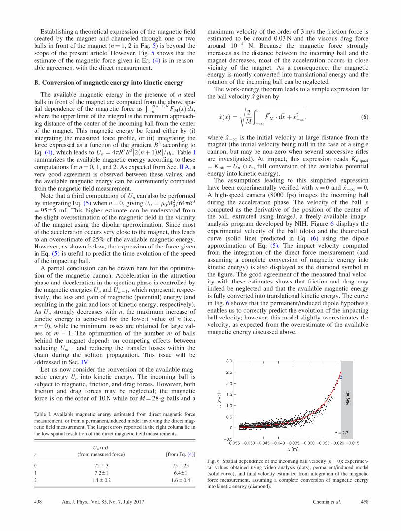
The assumptions leading to this simplified expressionhave been experimentally verified with n¼ 0 and _x�1 ¼ 0.A high-speed camera (8000 fps) images the incoming ballduring the acceleration phase. The velocity of the ball iscomputed as the derivative of the position of the center ofthe ball, extracted using ImageJ, a freely available image-analysis program developed by NIH. Figure 6 displays theexperimental velocity of the ball (dots) and the theoreticalcurve (solid line) predicted in Eq. (6) using the dipoleapproximation of Eq. (5). The impact velocity computedfrom the integration of the direct force measurement (andassuming a complete conversion of magnetic energy intokinetic energy) is also displayed as the diamond symbol inthe figure. The good agreement of the measured final veloc-ity with these estimates shows that friction and drag mayindeed be neglected and that the available magnetic energyis fully converted into translational kinetic energy. The curvein Fig. 6 shows that the permanent/induced dipole hypothesisenables us to correctly predict the evolution of the impactingball velocity; however, this model slightly overestimates thevelocity, as expected from the overestimate of the availablemagnetic energy discussed above.

Table I. Available magnetic energy estimated from direct magnetic force

measurement, or from a permanent/induced model involving the direct mag-

netic field measurement. The larger errors reported in the right column lie in

the low spatial resolution of the direct magnetic field measurements.

Un (mJ)

n (from measured force) [from Eq. (4)]

0 72 6 3 75 6 25

1 7:261 6:461

2 1.4 6 0.2 1.6 6 0.4

Fig. 6. Spatial dependence of the incoming ball velocity (n¼ 0): experimen-

tal values obtained using video analysis (dots), permanent/induced model

(solid curve), and final velocity estimated from integration of the magnetic

force measurement, assuming a complete conversion of magnetic energy

into kinetic energy (diamond).

498 Am. J. Phys., Vol. 85, No. 7, July 2017 Chemin et al. 498

As a partial conclusion here, we showed that the availablemagnetic energy from the attraction of the magnet is fullyconverted into translational kinetic energy. Moreover, weprovided a simplified expression of the force exerted by themagnet on the steel ball that leads to a theoretical expressionof the magnetic energy Un. Similar arguments can be appliedfor the ejection phase, where the kinetic energy of the ejectedball is given by Kfinal ¼ Keject � Um�1.

III. NESTERENKO SOLITON: FROM NEWTON’S

CRADLE TO GAUSS CRADLE

Following the impact of the incoming steel ball, the energypropagates in the ball chain similarly to what occurs inNewton’s cradle.12,13 However, in the magnetic cannon, thechain is inhomogeneous due to the presence of a sinteredNdFeB magnet. This section develops a classical model basedon Hertzian contact and discusses briefly the Nesterenko soli-ton. Experimental data accounting for the presence of the mag-net are then presented.

A. Nesterenko soliton: Propagation of a non-linear wave

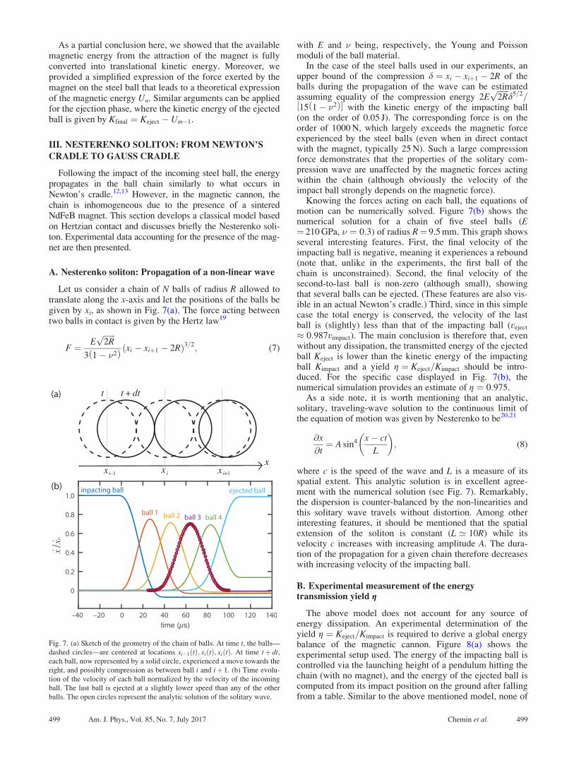
Let us consider a chain of N balls of radius R allowed totranslate along the x-axis and let the positions of the balls begiven by xi, as shown in Fig. 7(a). The force acting betweentwo balls in contact is given by the Hertz law19

F ¼ Effiffiffiffiffiffi2Rp

3 1� �2ð Þ xi � xiþ1 � 2Rð Þ3=2; (7)

with E and � being, respectively, the Young and Poissonmoduli of the ball material.

In the case of the steel balls used in our experiments, anupper bound of the compression d ¼ xi � xiþ1 � 2R of theballs during the propagation of the wave can be estimatedassuming equality of the compression energy 2E

ffiffiffiffiffiffi2Rp

d5=2=15 1� �2ð Þ½ � with the kinetic energy of the impacting ball

(on the order of 0.05 J). The corresponding force is on theorder of 1000 N, which largely exceeds the magnetic forceexperienced by the steel balls (even when in direct contactwith the magnet, typically 25 N). Such a large compressionforce demonstrates that the properties of the solitary com-pression wave are unaffected by the magnetic forces actingwithin the chain (although obviously the velocity of theimpact ball strongly depends on the magnetic force).

Knowing the forces acting on each ball, the equations ofmotion can be numerically solved. Figure 7(b) shows thenumerical solution for a chain of five steel balls (E¼ 210 GPa, � ¼ 0:3) of radius R¼ 9.5 mm. This graph showsseveral interesting features. First, the final velocity of theimpacting ball is negative, meaning it experiences a rebound(note that, unlike in the experiments, the first ball of thechain is unconstrained). Second, the final velocity of thesecond-to-last ball is non-zero (although small), showingthat several balls can be ejected. (These features are also vis-ible in an actual Newton’s cradle.) Third, since in this simplecase the total energy is conserved, the velocity of the lastball is (slightly) less than that of the impacting ball (veject

� 0:987vimpact). The main conclusion is therefore that, evenwithout any dissipation, the transmitted energy of the ejectedball Keject is lower than the kinetic energy of the impactingball Kimpact and a yield g ¼ Keject=Kimpact should be intro-duced. For the specific case displayed in Fig. 7(b), thenumerical simulation provides an estimate of g ¼ 0:975.

As a side note, it is worth mentioning that an analytic,solitary, traveling-wave solution to the continuous limit ofthe equation of motion was given by Nesterenko to be20,21

@x

@t¼ A sin4 x� ct

L

� �; (8)

where c is the speed of the wave and L is a measure of itsspatial extent. This analytic solution is in excellent agree-ment with the numerical solution (see Fig. 7). Remarkably,the dispersion is counter-balanced by the non-linearities andthis solitary wave travels without distortion. Among otherinteresting features, it should be mentioned that the spatialextension of the soliton is constant (L ’ 10R) while itsvelocity c increases with increasing amplitude A. The dura-tion of the propagation for a given chain therefore decreaseswith increasing velocity of the impacting ball.

B. Experimental measurement of the energytransmission yield g

The above model does not account for any source ofenergy dissipation. An experimental determination of theyield g ¼ Keject=Kimpact is required to derive a global energybalance of the magnetic cannon. Figure 8(a) shows theexperimental setup used. The energy of the impacting ball iscontrolled via the launching height of a pendulum hitting thechain (with no magnet), and the energy of the ejected ball iscomputed from its impact position on the ground after fallingfrom a table. Similar to the above mentioned model, none of

Fig. 7. (a) Sketch of the geometry of the chain of balls. At time t, the balls—

dashed circles—are centered at locations xi�1 tð Þ; xi tð Þ; xi tð Þ. At time tþ dt,each ball, now represented by a solid circle, experienced a move towards the

right, and possibly compression as between ball i and iþ 1. (b) Time evolu-

tion of the velocity of each ball normalized by the velocity of the incoming

ball. The last ball is ejected at a slightly lower speed than any of the other

balls. The open circles represent the analytic solution of the solitary wave.

499 Am. J. Phys., Vol. 85, No. 7, July 2017 Chemin et al. 499

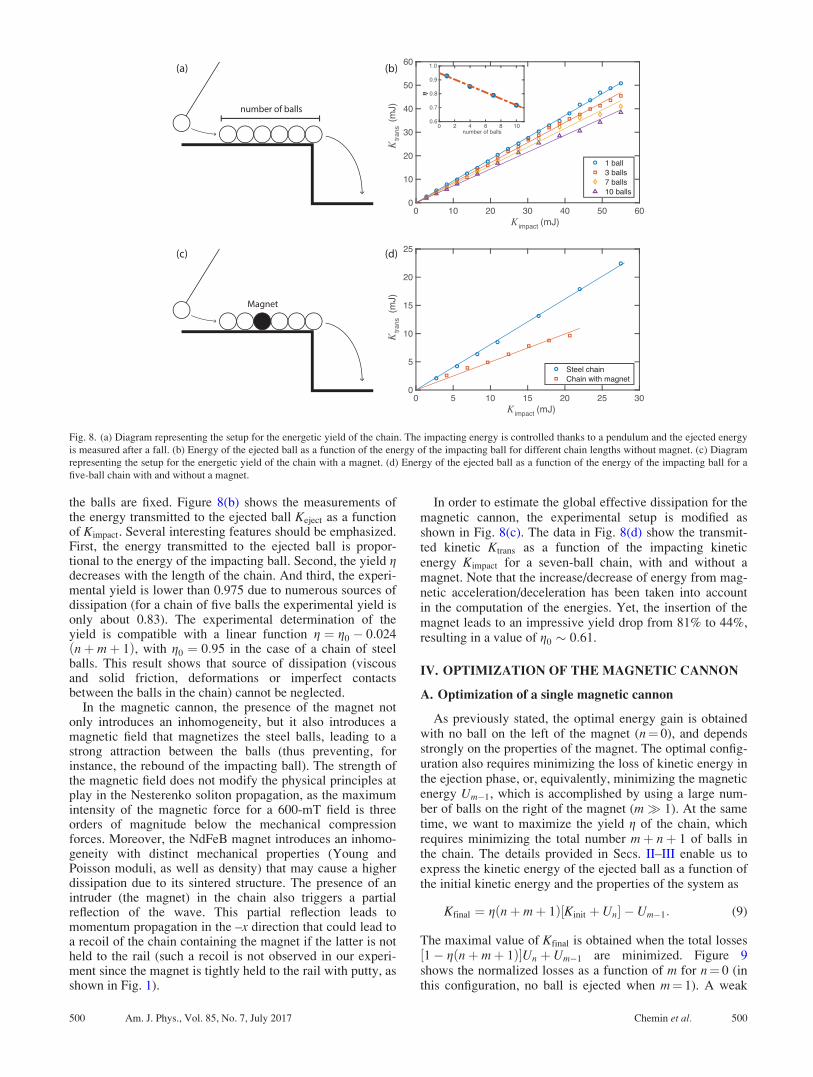
the balls are fixed. Figure 8(b) shows the measurements ofthe energy transmitted to the ejected ball Keject as a functionof Kimpact. Several interesting features should be emphasized.First, the energy transmitted to the ejected ball is propor-tional to the energy of the impacting ball. Second, the yield gdecreases with the length of the chain. And third, the experi-mental yield is lower than 0.975 due to numerous sources ofdissipation (for a chain of five balls the experimental yield isonly about 0.83). The experimental determination of theyield is compatible with a linear function g ¼ g0 � 0:024nþ mþ 1ð Þ, with g0 ¼ 0:95 in the case of a chain of steel

balls. This result shows that source of dissipation (viscousand solid friction, deformations or imperfect contactsbetween the balls in the chain) cannot be neglected.

In the magnetic cannon, the presence of the magnet notonly introduces an inhomogeneity, but it also introduces amagnetic field that magnetizes the steel balls, leading to astrong attraction between the balls (thus preventing, forinstance, the rebound of the impacting ball). The strength ofthe magnetic field does not modify the physical principles atplay in the Nesterenko soliton propagation, as the maximumintensity of the magnetic force for a 600-mT field is threeorders of magnitude below the mechanical compressionforces. Moreover, the NdFeB magnet introduces an inhomo-geneity with distinct mechanical properties (Young andPoisson moduli, as well as density) that may cause a higherdissipation due to its sintered structure. The presence of anintruder (the magnet) in the chain also triggers a partialreflection of the wave. This partial reflection leads tomomentum propagation in the –x direction that could lead toa recoil of the chain containing the magnet if the latter is notheld to the rail (such a recoil is not observed in our experi-ment since the magnet is tightly held to the rail with putty, asshown in Fig. 1).

In order to estimate the global effective dissipation for themagnetic cannon, the experimental setup is modified asshown in Fig. 8(c). The data in Fig. 8(d) show the transmit-ted kinetic Ktrans as a function of the impacting kineticenergy Kimpact for a seven-ball chain, with and without amagnet. Note that the increase/decrease of energy from mag-netic acceleration/deceleration has been taken into accountin the computation of the energies. Yet, the insertion of themagnet leads to an impressive yield drop from 81% to 44%,resulting in a value of g0 � 0:61.

IV. OPTIMIZATION OF THE MAGNETIC CANNON

A. Optimization of a single magnetic cannon

As previously stated, the optimal energy gain is obtainedwith no ball on the left of the magnet (n¼ 0), and dependsstrongly on the properties of the magnet. The optimal config-uration also requires minimizing the loss of kinetic energy inthe ejection phase, or, equivalently, minimizing the magneticenergy Um�1, which is accomplished by using a large num-ber of balls on the right of the magnet (m� 1). At the sametime, we want to maximize the yield g of the chain, whichrequires minimizing the total number mþ nþ 1 of balls inthe chain. The details provided in Secs. II–III enable us toexpress the kinetic energy of the ejected ball as a function ofthe initial kinetic energy and the properties of the system as

Kfinal ¼ g nþ mþ 1ð Þ Kinit þ Un½ � � Um�1: (9)

The maximal value of Kfinal is obtained when the total losses1� g nþ mþ 1ð Þ½ �Un þ Um�1 are minimized. Figure 9

shows the normalized losses as a function of m for n¼ 0 (inthis configuration, no ball is ejected when m¼ 1). A weak

Fig. 8. (a) Diagram representing the setup for the energetic yield of the chain. The impacting energy is controlled thanks to a pendulum and the ejected energy

is measured after a fall. (b) Energy of the ejected ball as a function of the energy of the impacting ball for different chain lengths without magnet. (c) Diagram

representing the setup for the energetic yield of the chain with a magnet. (d) Energy of the ejected ball as a function of the energy of the impacting ball for a

five-ball chain with and without a magnet.

500 Am. J. Phys., Vol. 85, No. 7, July 2017 Chemin et al. 500

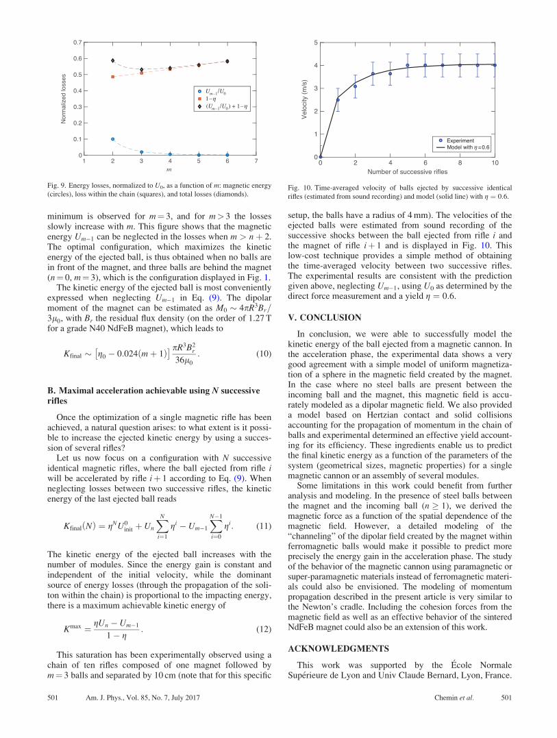
minimum is observed for m¼ 3, and for m> 3 the lossesslowly increase with m. This figure shows that the magneticenergy Um�1 can be neglected in the losses when m > nþ 2.The optimal configuration, which maximizes the kineticenergy of the ejected ball, is thus obtained when no balls arein front of the magnet, and three balls are behind the magnet(n¼ 0, m¼ 3), which is the configuration displayed in Fig. 1.

The kinetic energy of the ejected ball is most convenientlyexpressed when neglecting Um�1 in Eq. (9). The dipolarmoment of the magnet can be estimated as M0 � 4pR3Br=3l0, with Br the residual flux density (on the order of 1.27 Tfor a grade N40 NdFeB magnet), which leads to

Kfinal � g0 � 0:024 mþ 1ð Þ� � pR3B2

r

36l0

: (10)

B. Maximal acceleration achievable using N successive

rifles

Once the optimization of a single magnetic rifle has beenachieved, a natural question arises: to what extent is it possi-ble to increase the ejected kinetic energy by using a succes-sion of several rifles?

Let us now focus on a configuration with N successiveidentical magnetic rifles, where the ball ejected from rifle iwill be accelerated by rifle iþ 1 according to Eq. (9). Whenneglecting losses between two successive rifles, the kineticenergy of the last ejected ball reads

Kfinal Nð Þ ¼ gNU0init þ Un

XN

i¼1

gi � Um�1

XN�1

i¼0

gi: (11)

The kinetic energy of the ejected ball increases with thenumber of modules. Since the energy gain is constant andindependent of the initial velocity, while the dominantsource of energy losses (through the propagation of the soli-ton within the chain) is proportional to the impacting energy,there is a maximum achievable kinetic energy of

Kmax ¼ gUn � Um�1

1� g: (12)

This saturation has been experimentally observed using achain of ten rifles composed of one magnet followed bym¼ 3 balls and separated by 10 cm (note that for this specific

setup, the balls have a radius of 4 mm). The velocities of theejected balls were estimated from sound recording of thesuccessive shocks between the ball ejected from rifle i andthe magnet of rifle iþ 1 and is displayed in Fig. 10. Thislow-cost technique provides a simple method of obtainingthe time-averaged velocity between two successive rifles.The experimental results are consistent with the predictiongiven above, neglecting Um�1, using U0 as determined by thedirect force measurement and a yield g ¼ 0:6.

V. CONCLUSION

In conclusion, we were able to successfully model thekinetic energy of the ball ejected from a magnetic cannon. Inthe acceleration phase, the experimental data shows a verygood agreement with a simple model of uniform magnetiza-tion of a sphere in the magnetic field created by the magnet.In the case where no steel balls are present between theincoming ball and the magnet, this magnetic field is accu-rately modeled as a dipolar magnetic field. We also provideda model based on Hertzian contact and solid collisionsaccounting for the propagation of momentum in the chain ofballs and experimental determined an effective yield account-ing for its efficiency. These ingredients enable us to predictthe final kinetic energy as a function of the parameters of thesystem (geometrical sizes, magnetic properties) for a singlemagnetic cannon or an assembly of several modules.

Some limitations in this work could benefit from furtheranalysis and modeling. In the presence of steel balls betweenthe magnet and the incoming ball (n 1), we derived themagnetic force as a function of the spatial dependence of themagnetic field. However, a detailed modeling of the“channeling” of the dipolar field created by the magnet withinferromagnetic balls would make it possible to predict moreprecisely the energy gain in the acceleration phase. The studyof the behavior of the magnetic cannon using paramagnetic orsuper-paramagnetic materials instead of ferromagnetic materi-als could also be envisioned. The modeling of momentumpropagation described in the present article is very similar tothe Newton’s cradle. Including the cohesion forces from themagnetic field as well as an effective behavior of the sinteredNdFeB magnet could also be an extension of this work.

ACKNOWLEDGMENTS

This work was supported by the �Ecole NormaleSup�erieure de Lyon and Univ Claude Bernard, Lyon, France.

Fig. 9. Energy losses, normalized to U0, as a function of m: magnetic energy

(circles), loss within the chain (squares), and total losses (diamonds).Fig. 10. Time-averaged velocity of balls ejected by successive identical

rifles (estimated from sound recording) and model (solid line) with g ¼ 0:6.

501 Am. J. Phys., Vol. 85, No. 7, July 2017 Chemin et al. 501

The authors acknowledge also A. Bourges, C. Gouiller, A.Guittonneau, C. Malciu, G. Panel, and J. Sautel with whomdiscussions and exchanges were prolific. The authors wouldlike to emphasize that the work presented here was done inpreparation for the International Physicists Tournament (Ref.22), a world-wide competition for undergraduate students.The authors would highly recommend participation in theIPT as a rare learning opportunity for undergraduatestudents. The organization committee of the InternationalPhysicist Tournament is gratefully acknowledged, as arecontributions of the French Academy of Sciences and all theother tournament’s partners.

a)Electronic mail: nicolas.plihon@ens-lyon.fr1J. A. Rabchuk, “The Gauss rifle and magnetic energy,” Phys. Teach.

41(3), 158–161 (2003).2D. Kagan, “Energy and momentum in the gauss accelerator,” Phys. Teach.

42(1), 24–26 (2004).3O. Chittasirinuwat, T. Kruatong, and B. Paosawatyanyong, “More fun and

curiosity with magnetic guns in the classroom,” Phys. Educ. 46(3),

318–322 (2011).4C. Ucke and H.-J. Schlichting, “Die magnetkanone,” Phys. Unserer Zeit

40(3), 152–155 (2009).5S. O. Starr, R. C. Youngquist, and R. B. Cox, “A low voltage railgun,”

Am. J. Phys. 81(1), 38–43 (2013).6R. Casta~ner, J. M. Medina, and M. J. Cuesta-Bolao, “The magnetic dipole

interaction as measured by spring dynamometers,” Am. J. Phys. 74(6),

510–513 (2006).7N. Derby and S. Olbert, “Cylindrical magnets and ideal solenoids,” Am. J.

Phys. 78(3), 229–235 (2010).8R. S. Davis, “Using small, rare-earth magnets to study the susceptibility of

feebly magnetic metals,” Am. J. Phys. 60(4), 365–370 (1992).9B. S. N. Prasad, S. V. Shastry, and K. M. Hebbar, “An experiment to deter-

mine the relative permeability of ferrites,” Am. J. Phys. 40(6), 907–910

(1972).

10J. F. Borin and O. Baffa, “Measuring magnetic properties of ferromagnetic

materials,” Am. J. Phys. 66(5), 449–452 (1998).11W. M. Saslow, “How a superconductor supports a magnet, how magneti-

cally soft iron attracts a magnet, and eddy currents for the uninitiated,”

Am. J. Phys. 59(1), 16–25 (1991).12F. Herrmann and M. Seitz, “How does the ball-chain work?,” Am. J. Phys.

50(11), 977–981 (1982).13S. Hutzler, G. Delaney, D. Weaire, and F. MacLeod, “Rocking Newton’s

cradle,” Am. J. Phys. 72(12), 1508–1516 (2004).14D. Gugan, “Inelastic collision and the Hertz theory of impact,” Am. J.

Phys. 68(10), 920–924 (2000).15D. J. Griffiths, Introduction to Electrodynamics, 4th ed. (Pearson, Boston,

MA, 2013), pp. 373–381.16J. D. Jackson, Classical Electrodynamics, 3rd ed. (John Wiley & Sons,

New York, NY, 1998).17D. P. Jackson, “Dancing paperclips and the geometric influence on magne-

tization: A surprising result,” Am. J. Phys. 74(4), 272–279 (2006).18There are a number of affordable linear Hall effect sensors such as

AD22151 from Analog Devices, A1302 from Allegro Microsystems,

HAL401 from Micronas, or SS39/SS49 from Honeywell.19H. Hertz, “On the contact of elastic solids,” J. Reine Angew. Math. 92,

156–171 (1882).20S. Sen and M. Manciu, “Discrete Hertzian chains and solitons,” Physica A

268(3–4), 644–649 (1999).21V. F. Nesterenko, “Propagation of nonlinear compression pulses in granu-

lar media,” J. Appl. Mech. Tech. Phys. 24(5), 733–743 (1983).22More information on the International Physicists Tournament (IPT) can be

found at < http://iptnet.info >. Each national team is composed of six stu-

dents who work throughout the academic year on a list of seventeen open

questions and present their findings during the tournament. Unlike a typi-

cal physics exam, the problems must not only be presented, but also chal-

lenged and reviewed by the other participants, allowing students to

respectively assume the roles of researchers, referees, and editors. In addi-

tion to the challenge that the tournament represents, it provides students

with an exciting and eye-opening experience in which they learn how to

design experiments with the aim of solving physics problems, and to con-

structively criticize scientific solutions.

502 Am. J. Phys., Vol. 85, No. 7, July 2017 Chemin et al. 502