Code Area covered Resolution Reference 13.0 MF5 5 km Maus et al. (2007a) 101.41 Marine track-line variable NGDC, http://www.ngdc.noaa.gov/mgg/geodas/trackline.html 101.45 Interpolated (101.41) Non-interpolated (101.45) 121.43 Arctic 5 km Geoscience Canada, http://gsc.nrcan.gc.ca/index_e.php 131.45 Project Magnet variable NGDC, http://www.ngdc.noaa.gov/seg/geomag/proj_mag.shtml 171.44 Oceanic model 10 km NASA candidate model, accompanying DVD 201.2 Africa 15 min GETECH, http://www.getech.com 201.2 South America 15 min GETECH, http://www.getech.com 222.3 South Africa 5 km SADC, http://www.sadc.int 231.32 Botswana 5 km http://www.gov.bw/ 302.43 Antarctic 5 km ADMAP, http://earthsciences.osu.edu/admap 401.3 Eurasia 2 km Geoscience Canada, http://gsc.nrcan.gc.ca/index_e.php 411.43 East Asia 2 km CCOP, http://www.ccop.or.th 421.43 Middle East 1 km AAIME, http://home.casema.nl/errenwijlens/itc/aaime 441.3 India 5 km GSI, http://www.gsi.gov.in 442.2 India 50 km Qureshy, M.N., 1982, Photogrammetria, Vol. 37, 161-184 451.32 Japan 1 km http://www.aist.go.jp/GSJ/ 504.43 Australia 1 km Geoscience Australia, http://www.ga.gov.au 601.43 Europe 5 km Wonik, T. et al., 2001, Terra Nova, Vol 13, 203-213 611.3 Fennoscandia 5 km GTK, http://www.gtk.fi 621.321 Austria 5 km http://www.geologie.ac.at/ 622.2 Canary Islands 5 km Publ. Tec., No. 35, Instituto Geografico Nacional, Madrid, 1996 624.22 Finland 1 km http://projects.gtk.fi/WDMAM/ 625.2 France 10 km IPGP, http://www.ipgp.jussieu.fr 626.2 Italy 5 km Chiappini, M. et al., 2000, Annali di Geophysica, Vol 43, No.5 627.43 Spain 1.5 min Socias I., et al., 1991, Earth Planet. Sci. Lett., 105, 55-64 628.3 Russia 5 km VSEGEI, http://www.vsegei.ru/WAY/247038/locale/EN 701.43 North America 1 km NAMAG, http://pubs.usgs.gov/sm/mag_map 711.32 Mexico 5 km http://www.coremisgm.gob.mx/ 811.45 Argentina inland 5 km SEGEMAR, http://www.segemar.gov.ar/db 812.3 Argentina margin 5 km Instituto Antártico Argentino, http://ggt.conae.gov.ar/iaa/pictr2002

MAGNETIC ANOMALY MAP OF THE WORLD CARTE DES ANOMALIES MAGNÉTIQUES DU MONDE

EXPLANATORY NOTES / NOTICE EXPLICATIVE

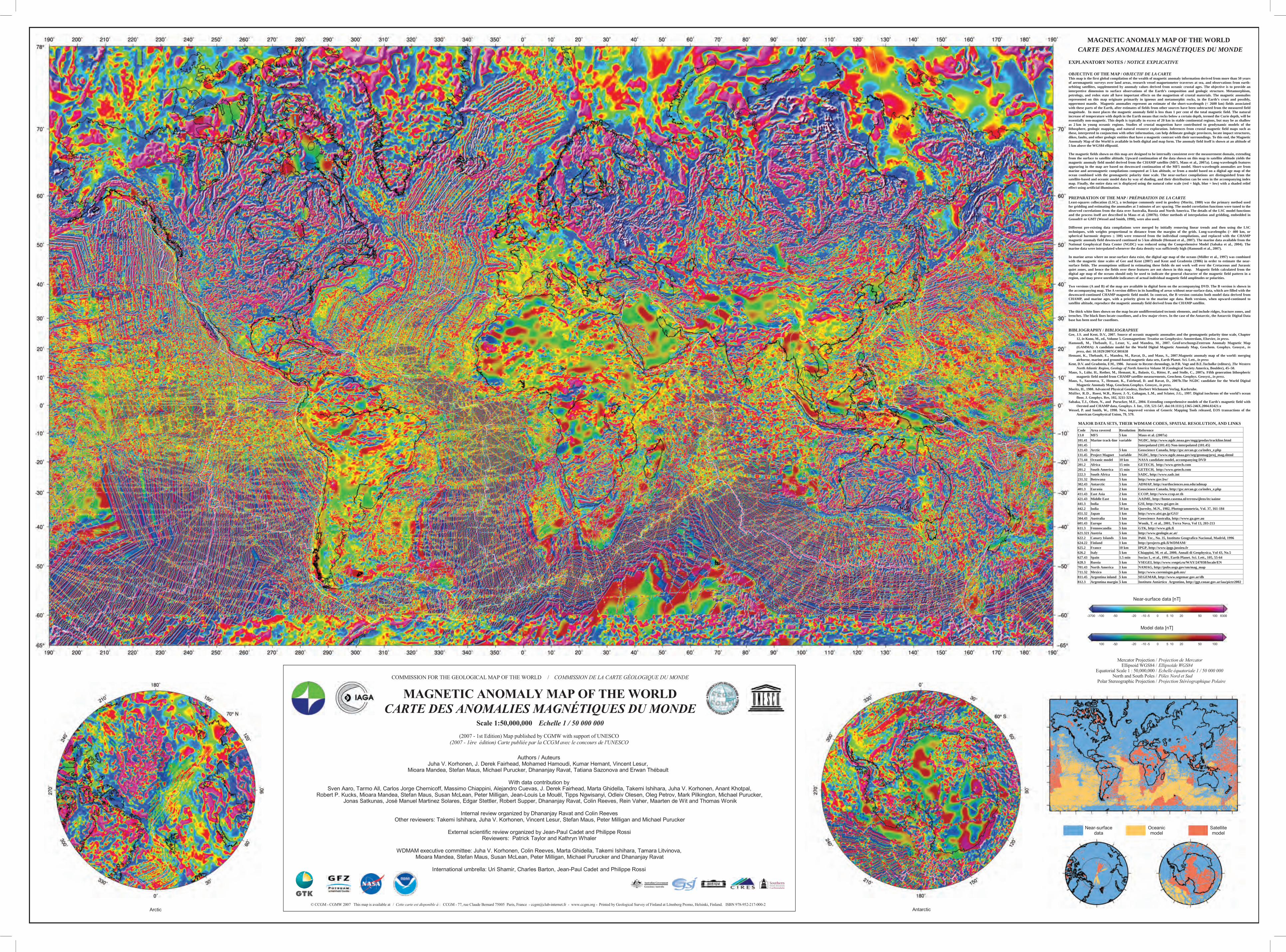
OBJECTIVE OF THE MAP / OBJECTIF DE LA CARTEThis map is the first global compilation of the wealth of magnetic anomaly information derived from more than 50 years of aeromagnetic surveys over land areas, research vessel magnetometer traverses at sea, and observations from earth-orbiting satellites, supplemented by anomaly values derived from oceanic crustal ages. The objective is to provide an interpretive dimension to surface observations of the Earth’s composition and geologic structure. Metamorphism, petrology, and redox state all have important effects on the magnetism of crustal materials. The magnetic anomalies represented on this map originate primarily in igneous and metamorphic rocks, in the Earth’s crust and possibly, uppermost mantle. Magnetic anomalies represent an estimate of the short-wavelength (< 2600 km) fields associated with these parts of the Earth, after estimates of fields from other sources have been subtracted from the measured field magnitude. In most places the magnetic anomaly field is less than 1 per cent of the total magnetic field. The natural increase of temperature with depth in the Earth means that rocks below a certain depth, termed the Curie depth, will be essentially non-magnetic. This depth is typically in excess of 20 km in stable continental regions, but may be as shallow as 2 km in young oceanic regions. Studies of crustal magnetism have contributed to geodynamic models of the lithosphere, geologic mapping, and natural resource exploration. Inferences from crustal magnetic field maps such as these, interpreted in conjunction with other information, can help delineate geologic provinces, locate impact structures, dikes, faults, and other geologic entities that have a magnetic contrast with their surroundings. To this end, the Magnetic Anomaly Map of the World is available in both digital and map form. The anomaly field itself is shown at an altitude of 5 km above the WGS84 ellipsoid.

The magnetic fields shown on this map are designed to be internally consistent over the measurement domain, extending from the surface to satellite altitude. Upward continuation of the data shown on this map to satellite altitude yields the magnetic anomaly field model derived from the CHAMP satellite (MF5, Maus et al., 2007a). Long-wavelength features appearing in the map are based on downward continuation of the MF5 model. Short-wavelength anomalies are from marine and aeromagnetic compilations computed at 5 km altitude, or from a model based on a digital age map of the ocean combined with the geomagnetic polarity time scale. The near-surface compilations are distinguished from the satellite-based and oceanic model data by way of shading, and their distribution can be seen in the accompanying index map. Finally, the entire data set is displayed using the natural color scale (red = high, blue = low) with a shaded relief effect using artificial illumination.

PREPARATION OF THE MAP / PRÉPARATION DE LA CARTELeast-squares collocation (LSC), a technique commonly used in geodesy (Moritz, 1980) was the primary method used for gridding and estimating the anomalies at 3 minutes of arc spacing. The model correlation functions were tuned to the observed correlations from the data over Australia, Russia and North America. The details of the LSC model functions and the process itself are described in Maus et al. (2007b). Other methods of interpolation and gridding, embedded in Geosoft® or GMT (Wessel and Smith, 1998), were also used.

Different pre-existing data compilations were merged by initially removing linear trends and then using the LSC techniques, with weights proportional to distance from the margins of the grids. Long-wavelengths (> 400 km, or spherical harmonic degrees < 100) were removed from the individual compilations, and replaced with the CHAMP magnetic anomaly field downward continued to 5 km altitude (Hemant et al., 2007). The marine data available from the National Geophysical Data Center (NGDC) was reduced using the Comprehensive Model (Sabaka et al., 2004). The marine data were interpolated whenever the data density was sufficiently high (Hamoudi et al., 2007).

In marine areas where no near-surface data exist, the digital age map of the oceans (Müller et al., 1997) was combined with the magnetic time scales of Gee and Kent (2007) and Kent and Gradstein (1986) in order to estimate the near-surface fields. The assumptions utilized in estimating these fields do not work well over the Cretaceous and Jurassic quiet zones, and hence the fields over these features are not shown in this map. Magnetic fields calculated from the digital age map of the oceans should only be used to indicate the general character of the magnetic field pattern in a region, and may prove unreliable indicators of actual individual magnetic field amplitudes or polarities.

Two versions (A and B) of the map are available in digital form on the accompanying DVD. The B version is shown in the accompanying map. The A version differs in its handling of areas without near-surface data, which are filled with the downward-continued CHAMP magnetic field model. In contrast, the B version contains both model data derived from CHAMP, and marine ages, with a priority given to the marine age data. Both versions, when upward-continued to satellite altitude, reproduce the magnetic anomaly field derived from the CHAMP satellite.

The thick white lines shown on the map locate undifferentiated tectonic elements, and include ridges, fracture zones, and trenches. The black lines locate coastlines, and a few major rivers. In the case of the Antarctic, the Antarctic Digital Data base has been used for coastlines.

BIBLIOGRAPHY / BIBLIOGRAPHIEGee, J.S. and Kent, D.V., 2007. Source of oceanic magnetic anomalies and the geomagnetic polarity time scale, Chapter

12, in Kono, M., ed., Volume 5. Geomagnetism: Treatise on Geophysics: Amsterdam, Elsevier, in press.Hamoudi, M., Thebault, E., Lesur, V., and Mandea, M., 2007. GeoForschungsZentrum Anomaly Magnetic Map

(GAMMA): A candidate model for the World Digital Magnetic Anomaly Map, Geochem. Geophys. Geosyst., in press, doi: 10.1029/2007GC001638

Hemant, K., Thebault, E., Mandea, M., Ravat, D., and Maus, S., 2007.Magnetic anomaly map of the world: merging airborne, marine and ground-based magnetic data sets, Earth Planet. Sci. Lett., in press

Kent, D.V. and Gradstein, F.M., 1986. Jurassic to Recent chronology, in P.R. Vogt and B.E.Tucholke (editors), The Western North Atlantic Region, Geology of North America Volume M (Geological Society America, Boulder), 45–50.

Maus, S., Lühr, H., Rother, M., Hemant, K., Balasis, G., Ritter, P., and Stolle, C., 2007a. Fifth generation lithospheric magnetic field model from CHAMP satellite measurements, Geochem. Geophys. Geosyst., in press.

Maus, S., Sazonova, T., Hemant, K., Fairhead, D. and Ravat, D., 2007b.The NGDC candidate for the World Digital Magnetic Anomaly Map, Geochem.Geophys. Geosyst., in press.

Moritz, H., 1980. Advanced Physical Geodesy, Herbert Wichmann Verlag, Karlsruhe.Müller, R.D., Roest, W.R., Royer, J.-Y., Gahagan, L.M., and Sclater, J.G., 1997. Digital isochrons of the world’s ocean

floor, J. Geophys. Res, 102, 3211-3214.Sabaka, T.J., Olsen, N., and Purucker, M.E., 2004. Extending comprehensive models of the Earth's magnetic field with

Oersted and CHAMP data, Geophys. J. Int., 159, 521-547, doi:10.1111/j.1365-246X.2004.02421.xWessel, P. and Smith, W., 1998. New, improved version of Generic Mapping Tools released, EOS transactions of the

American Geophysical Union, 79, 579.

MAJOR DATA SETS, THEIR WDMAM CODES, SPATIAL RESOLUTION, AND LINKS

_