Embed Size (px)
Citation preview

WORK ING PAPER SER I E SNO 1382 / S EPTEMBER 2011
by Peter Sarlinand Tuomas A. Peltonen
MAPPING THESTATE OFFINANCIAL STABILITY
MACROPRUDENTIALRESEARCH NETWORK
1 The authors want to thank the anonymous referee, Barbro Back, Tomas Eklund, Kristian Koerselman, Marco Lo Duca, Fredrik Lucander, and seminar participants at the ESCB Macro-Prudential Research Network (MaRs) workshop on 14–15 April 2011 in Frankfurt am Main, the
International Joint Conference on Artificial Intelligence (IJCAI’11) workshop on Chance Discovery on 16–22 July 2011 in Barcelona, the Bank of Finland Institute for Economies in Transition (BOFIT) and the Data Mining and Knowledge Management Laboratory
at Åbo Akademi University for useful comments and discussions. All remaining errors are of our own.2 Åbo Akademi University, Turku Centre for Computer Science, Joukahaisenkatu 3–5, 20520 Turku, Finland; e-mail: [email protected].
3 European Central Bank, Kaiserstrasse 29, D-6031, Frankfurt am Main, Germany; e-mail: [email protected].
This paper can be downloaded without charge from http://www.ecb.europa.eu or from the Social Science Research Network electronic library at http://ssrn.com/abstract_id=1914294.
NOTE: This Working Paper should not be reported as representing the views of the European Central Bank (ECB). The views expressed are those of the authors
and do not necessarily reflect those of the ECB.
Working PaPer Ser ie Sno 1382 / SePtember 2011
maPPing the State of financial Stability 1
by Peter Sarlin 2 and Tuomas A. Peltonen 3
In 2011 all ECB publications
feature a motif taken from
the €100 banknote.
MACROPRUDENTIALRESEARCH NETWORK
© European Central Bank, 2011
AddressKaiserstrasse 2960311 Frankfurt am Main, Germany
Postal addressPostfach 16 03 1960066 Frankfurt am Main, Germany
Telephone+49 69 1344 0
Internethttp://www.ecb.europa.eu
Fax+49 69 1344 6000
All rights reserved.
Any reproduction, publication and reprint in the form of a different publication, whether printed or produced electronically, in whole or in part, is permitted only with the explicit written authorisation of the ECB or the authors.
Information on all of the papers published in the ECB Working Paper Series can be found on the ECB’s website, http://www.ecb.europa.eu/pub/scientific/wps/date/html/index.en.html
ISSN 1725-2806 (online)
Macroprudential Research Network
This paper presents research conducted within the Macroprudential Research Network (MaRs). The network is composed of economists from the European System of Central Banks (ESCB), i.e. the 27 national central banks of the European Union (EU) and the European Central Bank. The objective of MaRs is to develop core conceptual frameworks, models and/or tools supporting macro-prudential supervision in the EU.
The research is carried out in three work streams: 1) Macro-financial models linking financial stability and the
performance of the economy; 2) Early warning systems and systemic risk indicators; 3) Assessing contagion risks.
MaRs is chaired by Philipp Hartmann (ECB). Paolo Angelini (Banca d’Italia), Laurent Clerc (Banque de France), Carsten Detken (ECB) and Katerina Šmídková (Czech National Bank) are workstream coordinators. Xavier Freixas (Universitat Pompeu Fabra) acts as external consultant and Angela Maddaloni (ECB) as Secretary.
The refereeing process of this paper has been coordinated by a team composed of Cornelia Holthausen, Kalin Nikolov and Bernd Schwaab (all ECB).
The paper is released in order to make the research of MaRs generally available, in preliminary form, to encourage comments and suggestions prior to final publication. The views expressed in the paper are the ones of the author(s) and do not necessarily reflect those of the ECB or of the ESCB.

3ECB
Working Paper Series No 1382September 2011
Abstract 4
Non-technical summary 5
1 Introduction 6
2 Methodology 8
3 Self-organizing fi nancial stability map 13
4 Mapping the state of fi nancial stability 17
5 Conclusions 18
Annex 20
References 22
Tables and fi gures 25
CONTENTS

4ECBWorking Paper Series No 1382September 2011
Abstract
The paper uses the Self-Organizing Map for mapping the state of financial stability and visualizing the sources of systemic risks as well as for predicting systemic financial crises. The Self-Organizing Financial Stability Map (SOFSM) enables a two-dimensional representation of a multidimensional financial stability space that allows disentangling the individual sources impacting on systemic risks. The SOFSM can be used to monitor macro-financial vulnerabilities by locating a country in the financial stability cycle: being it either in the pre-crisis, crisis, post-crisis or tranquil state. In addition, the SOFSM performs better than or equally well as a logit model in classifying in-sample data and predicting out-of-sample the global financial crisis that started in 2007. Model robustness is tested by varying the thresholds of the models, the policymaker’s preferences, and the forecasting horizons. JEL Codes: E44, E58, F01, F37, G01. Keywords: systemic financial crisis, systemic risk, Self-Organizing Map (SOM), visualization, prediction, macroprudential supervision
5ECB
Working Paper Series No 1382September 2011
Non-technical summary
The recent global financial crisis has demonstrated the importance of understanding sources of domestic and global vulnerabilities that may lead to a systemic financial crisis. Early identification of sources of vulnerability is important as it would allow introduction of policy actions to decrease further build up of vulnerabilities or enhance the shock absorption capacity of the financial system. Much of the empirical literature deals with early warning systems (EWSs) that rely on conventional statistical modelling methods, such as the univariate ‘signals’ approach or multivariate logit/probit models. Given the changing nature of financial crises, stand-alone numerical predictions are unlikely to be able to thoroughly describe them. As a complement to numerical predictions, this motivates the development of tools with clear visual capabilities, enabling real human perception. Dimensionality of the problem complicates visualization, since a large number of indicators are often required to accurately assess vulnerabilities to a financial crisis. In addition to the limitation of standard two- and three-dimensional visualizations in describing higher dimensions, there are challenges of including a temporal or cross-sectional dimension. Moreover, while composite indices of leading indicators and predicted probabilities as outputs of EWSs enable comparison across countries and over time, such indices fall short in representing sub-dimensions of the problem. Methods for exploratory data analysis can to some extent overcome these types of shortcomings. Exploratory data analysis attempts to describe the phenomena of interest in easily understandable forms by illustrating the structures in data. The Self-Organizing Map (SOM) is a method that combines the aims of projection and clustering techniques. It can provide an easily interpretable non-linear description of the multidimensional data distribution on a two-dimensional plane without losing sight of individual indicators. Thus, the two-dimensional output of the SOM makes it particularly useful for static visualizations, or summarizations, of large amounts of information. This paper describes a methodology to map the state of financial stability and the sources of systemic risks. The Self-Organizing Financial Stability Map (SOFSM) enables a two-dimensional representation of a multidimensional financial stability space and allows disentangling the individual sources of vulnerabilities impacting on systemic risks. The map can be used to monitor macro-financial vulnerabilities by locating a particular country in the financial stability cycle: being it either in the pre-crisis, crisis, post-crisis or tranquil state. In addition, the SOFSM model performs as well or better than a logit model in classifying in-sample data and predicting out-of-sample the global financial crisis that started in 2007. Robustness of the SOFSM is tested by varying the thresholds of the models, policymaker preferences, and the forecasting horizon.
6ECBWorking Paper Series No 1382September 2011
1. Introduction
The recent global financial crisis has demonstrated the importance of understanding sources of domestic and global vulnerabilities that may lead to a systemic financial crisis.4 Early identification of financial stress would allow policymakers to introduce policy actions to decrease or prevent further build up of vulnerabilities or otherwise enhance the shock absorption capacity of the financial system. Finding the individual sources of vulnerability and risk is of central importance since that allows targeted actions for repairing specific cracks in the financial system. Much of the empirical literature deals with early warning systems (EWSs) that rely on conventional statistical modelling methods, such as the univariate signals approach or multivariate logit/probit models.5 However, financial crises are complex events driven by non-linearly related and non-normally distributed economic and financial factors.6 These non-linearities derive, for example, from the fact that crises become more likely as the number of fragilities increase. Due to distributional assumptions, conventional statistical techniques may fail in modelling these events. Novel EWSs attempt to model these complex relationships by applying non-linear techniques (Demyanyk and Hasan, 2010). For example, Peltonen (2006) and Fioramanti (2008) show that a neural network outperforms a probit model in predicting currency and debt crises. However, while the utilization of non-linear techniques may increase a posteriori prediction accuracies to a minor extent, Peltonen (2006) and Berg et al. (2005) demonstrate that the results of a priori predictions of financial crises remain disappointing. Given the changing nature of the occurrences of these extreme events, stand-alone numerical analyzes are unlikely to comprehensively describe them. As a complement, this motivates the development of tools with clear visual capabilities and intuitive interpretability, enabling real human perception. One reason interpretability of the monitoring systems has not been adequately addressed is the complexity of the problem. A large number of indicators are often required to accurately assess the sources of financial instability. As with raw statistical tables, standard two- and three-dimensional visualizations have, of course, their limitations for high dimensions, not to mention the challenge of including a temporal or cross-sectional dimension or assessing multiple countries over time. Although composite indices of leading indicators and predicted probabilities of EWSs enable comparison across countries and over time, these indices fall short in disentangling the sources of vulnerability.7 The recent work by IMF staff on the Global Financial Stability Map (GFSM) (Dattels et al., 2010) has sought to overcome this challenge by a mapping of six composite indices.8 Even here, however, the GFSM spider chart
4 Cardarelli et al. (2011) show that out of 113 financial stress episodes for 17 key advanced economies, 29 were followed by an economic slowdown and an equal number by recessions. 5 Logit and probit models have been applied frequently to predicting financial crises. For example, Berg and Pattillo (1999) apply a discrete choice model to predicting currency crises; Fuertes and Kalotychou (2006) to predicting debt crises; and Lo Duca and Peltonen (2011) to predicting systemic crises. An exception is the univariate non-parametric indicator proposed by Kaminsky et al. (1998), and its subsequent versions. See Berg et al. (2005) for a comprehensive review. 6 Fioramanti (2008), Sarlin and Marghescu (2009) and Lo Duca and Peltonen (2011) show that indicators of debt, currency, and systemic crises are non-linearly related. 7 There exist several composite indices for measuring financial tensions, e.g. Illing and Liu (2006), Cardarelli et al. (2011) and Lo Duca and Peltonen (2011). These will be further discussed in Section 2. 8 The GFSM has appeared quarterly in the Global Financial Stability Report (GFSR) since April 2007.

7ECB
Working Paper Series No 1382September 2011
4
visualization of six indices falls short in disentangling individual sources. Familiar limitations of spider charts are, for example, the facts that area does not scale one-to-one with increases in variables and that the area itself depends on the order of dimensions. In addition, the use of adjustment based on market and domain intelligence, especially during crisis episodes, and the absence of a systematic evaluation gives neither a transparent data-driven measure of financial stress nor an objective anticipation of the GFSM’s future precision. Indeed, the GFSM comes with the following caveat: “given the degree of ambiguity and arbitrariness of this exercise the results should be viewed merely illustrative”.9 Methods for exploratory data analysis such as projection and clustering techniques may help in overcoming these shortcomings by illustrating data structures in easily understandable forms. The Self-Organizing Map (SOM) (Kohonen, 1982; 2001) is a method that combines the aims of projection and clustering techniques. It is capable of providing an easily interpretable non-linear description of the multidimensional data distribution on a two-dimensional plane without losing sight of individual indicators. The two-dimensional output of the SOM makes it particularly useful for static visualizations, or summarizations, of large amounts of information (Back et al., 1998). By 2005, over 7700 works had featured the SOM (Pöllä et al., 2009). While extensively applied to topics in engineering and medicine, the literature is short of thorough testing of the SOM for financial stability monitoring. In the emerging market context, Arciniegas and Arciniegas Rueda (2009), Sarlin (2011), Sarlin and Marghescu (2011) and Resta (2009) have applied the SOM to indicators of currency crises, debt crises and general economic and financial performance, respectively. The SOM has not, to our knowledge, been earlier applied to monitoring systemic risk or assessing the global dimensions of financial stability, including global macro-financial proxies as well as individual advanced and emerging market economies. Indeed, of the above applications, only Sarlin and Marghescu (2011) perform a thorough, systematic evaluation of the model’s predictive capabilities. The main contribution of this paper is to lay out a methodology for mapping the state of financial stability on a two-dimensional plane. As an enhancement to the GFSM approach, the Self-Organizing Financial Stability Map (SOFSM) not only allows disentangling the individual sources of vulnerability, but also performs well as an EWS in predicting out-of-sample systemic financial crises. The SOFSM parameter values for the final model are chosen based on a training framework aiming at a parsimonious, objective and interpretable model. Robustness of the SOFSM is tested by varying the thresholds of the models, policymaker preferences, and the forecasting horizon. In addition, when assessing a topologically ordered SOFSM, the concept of a financial stability neighborhood represents contagion of instabilities through similarities in the current macro-financial conditions. That is, a crisis in one position
9 The authors state that the definitions of starting and ending dates of the assessed crisis episodes are arbitrary. Similarly, the assessed crisis episodes are arbitrary, as some episodes in between the assessed ones are disregarded, such as Russia’s default in 1999 and the collapse of Long-Term Capital Management. Introduction of judgment based on market intelligence and technical adjustments are motivated when the GFSM is “unable to fully account for extreme events surpassing historical experience”, which is indeed an obstacle for empirical models, but also a factor of uncertainty in terms of future performance since nothing assures manual detection of vulnerabilities, risks and triggers.

8ECBWorking Paper Series No 1382September 2011
on the map indicates propagation of financial distress to adjacent locations. This type of representation may help in identifying the changing nature of crises. Further, inspired by Minsky’s (1982) and Kindleberger’s (1996) vindicated financial fragility view of a credit or asset cycle, we introduce the notion of the financial stability cycle. We show how the SOFSM can be used to monitor macro-financial vulnerabilities by locating a country in the financial stability cycle: being it either in the pre-crisis, crisis, post-crisis or tranquil state. We visualize samples of the panel dataset, cross-sectional and temporal data, on the two-dimensional map, and compute and visualize aggregates for the world, emerging market economies and advanced economies. The SOFSM enables disentangling the specific threats, risks and triggers, and should be treated as a starting point rather than an ending point for financial stability analysis. The paper is structured as follows. Section 2 introduces the SOM, the data and the evaluation framework. We present the training process and evaluation of the SOFSM in Section 3, and provide visual analyzes in Section 4. Section 5 concludes. 2. Methodology This section introduces SOMs in general and explains the model used in this paper. We also present the data set as well as the evaluation framework for the models in this section. Self-Organizing Maps (SOMs) Methods for exploratory data analysis fall, in general, into two groups: data and dimensionality reduction methods. Clustering methods attempt to reduce the amount of data by enabling analysis of a few mean profiles (clusters), but do not seek to project data to an easily interpretable format. Dimensionality reduction methods, e.g. Sammon’s (1969) mapping and its variants (Cox and Cox, 2001), project high-dimensional data onto a lower dimension, while attempting to preserve the structure of the dataset. Unlike clustering methods, however, projection methods do not generally seek to reduce or distil the amount of presented data. The SOM combines the objectives of projection and clustering techniques. The SOM is a projection and clustering tool that uses an unsupervised learning method developed by Kohonen (1982). It differs from projection techniques like multidimensional scaling by performing a mapping from the input data space onto a k-dimensional array of output nodes instead of into a continuous space and by attempting to preserve the neighbourhood relations in data rather than absolute distances. The vector quantization capability of the SOM allows modelling from the continuous space , with a probability density function f(x), to the grid of nodes, whose location depend on the neighbourhood structure of the data . On a two-dimensional grid, for example, the numbers on the x- and y-axes do not carry a numeric meaning in a parametric sense; they represent positions in the data space of the map, where each of these positions (x,y) is a mean profile. As proposed in Vesanto and Alhoniemi (2000), a second-level clustering can be applied on the nodes of the SOM, i.e. separation of data into nodes and nodes into clusters. They show that, compared to other clustering methods, the two-level SOM enhances the clustering through greater robustness on non-normally distributed data and the dual advantage of efficiency and speed. In Marghescu (2007), the data visualization features of the two-level SOM

9ECB
Working Paper Series No 1382September 2011
have been reviewed as better than those of other techniques. Information products of two-level SOMs have also been evaluated as superior than currently used methods by end-users within the domain of financial analysis (Eklund et al., 2008). The intuition of the basic SOM algorithm is presented here. See the Annex for further details on the SOM implementation used in this paper and Kohonen (2001) for a broad overview of the SOM. This paper uses a linearly initialized batch SOM algorithm with a Euclidean metric. The SOM grid consists of a user specified number of nodes im (where i=1,2,…,M), which are so-called reference vectors representing the same dimensions (number of variables) as the actual data set . Generally, the SOM algorithm operates according to the following steps (see the Annex for details of the steps):
1. Initialize the node values using the two principal components 2. Compare all data points jx with all nodes im to find for each data point the
nearest node bm (i.e., best-matching unit, BMU) 3. Update each node im to averages of the attracted data, including with
diminishing weight data located in a specified neighborhood 4. Repeat steps 2 and 3 a specified number of times 5. Group nodes into a reduced number of clusters using Ward’s (1963)
hierarchical clustering. The SOM parameters are radius of the neighbourhood , number of nodes M, map format (ratio of X and Y dimensions), and number of training iterations t. Large radii result in stiff maps that stress topology preservation at the cost of quantization accuracy, while updates based upon solely attracted data ( =0) leads to a standard k-means clustering with no topology preserving mapping. For the purpose of this analysis, the output of the SOM algorithm is visualized on a two-dimensional plane. The rationale for not using a one-dimensional map is differences within clusters. A three-dimensional map, while adding a further dimension, impairs the interpretability of data visualizations. Here, the multidimensional space of the grid is visualized through layers, or “feature planes”. For each individual indicator, a feature plane represents the distribution of its values on the two-dimensional map. As the feature planes are different views of the same map, one unique point represents the same node on all planes. We produce the feature planes in colour. Cold to warm colours represent low to high values of the indicator according to a colour scale below each feature plane. Shading on the two-dimensional map indicates the distance between each node and its corresponding second-level cluster centre, i.e. those close to the centre have a lighter shade and those farther away have a darker shade. The quality of the map is usually measured in terms of quantization error, distortion measure and topographic error (see e.g. Vesanto et al., 2003). As we have class information, we mainly use classification performance measures for evaluating the quality of the map.

10ECBWorking Paper Series No 1382September 2011
Data The data set used in this paper is the same as that in Lo Duca and Peltonen (2011). It consists of a database of systemic events and a set of vulnerability indicators commonly used in the macroprudential literature to predict financial crises. The quarterly dataset consists of 28 countries (10 advanced and 18 emerging economies) for the period 1990:1–2010:3. The data are retrieved from Haver Analytics, Bloomberg and Datastream. This section explains how systemic events are identified, how the financial stability cycle is constructed as well as how vulnerability indicators are created and chosen. Following Lo Duca and Peltonen (2011), the identification of systemic financial crises is done using a Financial Stress Index (FSI). This approach provides an objective criterion for the definition of the starting date of a systemic financial crisis.10 The idea behind the FSI is that the larger and broader the shock is (i.e. the more systemic the shock), the higher the co-movement among variables reflecting tensions in different market segments. By aggregating variables to an index that measures stresses across market segments, the FSI captures the starting and ending points of a systemic financial crisis. The FSI is a country-specific composite index that covers the main segments (money market, equity market and foreign exchange market) of the domestic financial market: (1) the spread of the 3-month interbank rate over the 3-month government bill rate (Ind1); (2) negative quarterly equity returns (Ind2); (3) the realized volatility of the main equity index (as average daily absolute changes over a quarter) (Ind3); (4) the realized volatility of the nominal effective exchange rate (Ind4); and (5) the realized volatility of the yield on the 3-month government bill (Ind5).11 Each indicator j (Indj) of the FSI for country i at quarter t is transformed into an integer from 0 to 3 according to the quartile of the country-specific distribution, while the transformed variable is denoted as )( ,,,, tijtij Indq . For example, a value for indicator j falling into the third quartile of the distribution would be transformed to a “2”. The FSI is computed for country i at time t as a simple average of the transformed variables as follows:
5
)(5
1,,,,
,j
tijtij
ti
IndqFSI (1)
To define systemic financial crises, the FSI is first transformed into a binary variable. In order to capture the systemic nature of the financial stress episodes, we focus on episodes of extreme financial stress that have led in the past (on average) to negative consequences for the real economy. In practice, we create a binary “crisis” variable, denoted as C0 that takes a value 1 in the quarter when the FSI moves above the
10 There are several composite indices for measuring financial tensions. For example, Illing and Liu (2006) and Hakkio and Keeton (2009). Cardarelli et al. (2011) and Balakrishnan et al. (2009) constructed financial stability indices for a broad set of advanced and emerging economies. 11 When the 3-month government bill rate is not available, the spread between interbank and T-bill rates of the closest maturity is used. The equity returns are multiplied by minus one, so that negative returns increase stress, while positive returns are set to 0. When computing realized volatilities for components Ind3-5, average daily absolute changes over a quarter are used.
11ECB
Working Paper Series No 1382September 2011
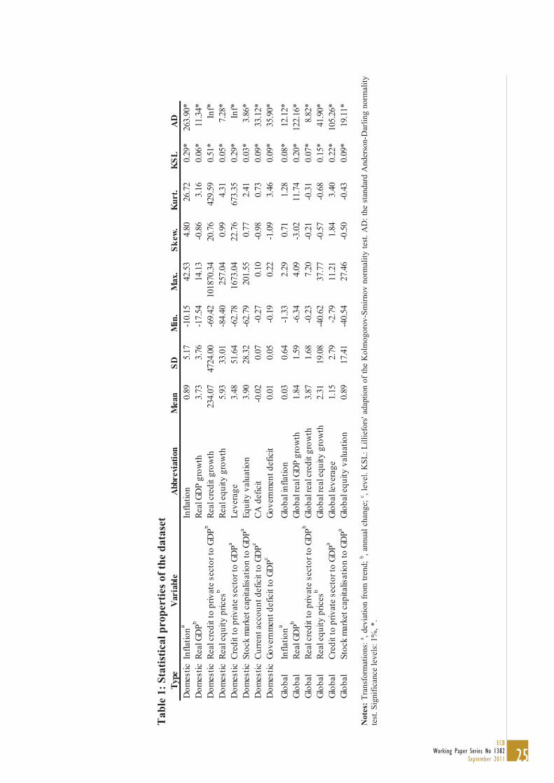
predefined threshold of the 90th percentile of its country-specific distribution and 0 otherwise. This approach identifies a set of 94 systemic events over 1990–2010. To describe the financial stability cycle, we create a set of other class variables besides to the crisis variable. First, a “pre-crisis” class variable C18 is created by setting the binary variable to 1 in the 18 months preceding the systemic financial crisis, and to 0 in all other periods. The pre-crisis variable mimics an ideal leading indicator that perfectly signals a systemic financial crisis in the 18 months before the event. In order to evaluate robustness for different horizons, we also create other pre-crisis class variables, by setting the binary variables C24, C12 and C6 to 1 in the 24, 12 and 6 months before the systemic event and zero otherwise. Similarly, we create “post-crisis” class variables P6, P12, P18 and P24 that are set to 1 in the 6, 12, 18 and 24 months after the systemic event. Finally, all other time periods are “tranquil” periods denoted as T0. To analyze the sources of systemic risk and vulnerability, we use the same indicators as in Lo Duca and Peltonen (2011). The set of indicators consists of commonly used metrics in the macroprudential literature for capturing the build-up of vulnerabilities and imbalances in the domestic and global economy (e.g. Borio and Lowe, 2002; 2004; Alessi and Detken, 2011). Our key variables are asset price developments and valuations, and variables proxying for credit developments and leverage. In addition, traditional variables (e.g. government budget deficit and current account deficit) are used to control for vulnerabilities stemming from macroeconomic imbalances.12 Following the literature, we construct several transformations of the indicators (e.g. annual changes and deviations from moving averages or trends) to proxy for misalignments and a build up of vulnerabilities. To proxy for global macro-financial imbalances and vulnerabilities, we calculate a set of global indicators by averaging the transformed variables for the United States, the euro area, Japan and the United Kingdom.13 The final set of indicators are chosen based on their univariate performance in predicting systemic events and are shown in Table 1. Statistical properties of the chosen indicators (Table 1) reveal that the data are significantly skewed and non-mesokurtic, and thus do not exhibit normal distributions. To take into account cross-country differences and country-specific fixed effects, we follow Kaminsky et al. (1998) by measuring indicators in terms of country-specific percentiles. While such outlier trimming is unnecessary for the clustering of the SOM, an even distribution is highly desirable for visualization. Finally, the analysis is conducted in a real-time fashion to the extent possible. Thus, we take into account publication lags by using lagged variables. For GDP, money and credit related indicators, the lag ranges from 1 to 2 quarters depending on the country. We also de-trend variables and measure indicators in terms of country-specific percentiles using the latest available information.
(See Table 1) 12 While Peltonen and Lo Duca (2011) include interaction terms of both domestic and global vulnerability indicators, we do not replicate them since they are included in the SOM processing per se. 13 Qualitatively similar results are obtained when global variables are constructed as simple averages of variables of all countries in the sample.

12ECBWorking Paper Series No 1382September 2011
Model evaluation framework This section presents the framework, which is used to evaluate the performance of models in terms of predicting systemic financial crises. As we have class information, we mainly use classification performance measures for finding the optimal model rather than the traditional SOM quality measures. We classify the outcomes into combinations of predicted and actual classes using a contingency matrix.
Actual class 1 -1
1 True positive (TP) False positive (FP) Predicted class
-1 False negative (FN) True negative (TN) Based on the elements of the matrix, we compute ratios for measuring performance: recall, precision, False Positive (FP), True Positive (TP), False Negative (FN) and True Negative (TN) rates, and overall accuracy.14 Due to unbalanced class sizes and differences in class importance, the above measures are sometime unsuited to summarize evaluations of crisis predictions. By assigning every object to the tranquil class, we would achieve a useless classifier for policy action, but still a high proportion of correct predictions (80%). This motivates using a common measure in information retrieval for evaluating performance on unbalanced class sizes. Matthews Correlation Coefficient (MCC) (Matthews, 1975) measures the correlation between the actual and predicted classes. It is defined in the range [-1,1], where -1 represents an inverse prediction and 1 a perfect prediction.15 The costs of FNs and FPs might be asymmetric, where the weight depends on the policymaker’s preferences between giving false signals of crisis and tranquil periods. To calibrate an optimal model and threshold for policy action, we adapt the approach pioneered in Demirgüç-Kunt and Detragiache (2000) with the technical implementation suggested by Alessi and Detken (2011). The loss function of the policymaker is thus defined as:
))/()(1())/(()( TNFPFPTPFNFNL , (2) where the parameter represents the relative preference of the policymaker between FNs and FPs. When 5.0 , the policymaker is equally concerned about missing crises and issuing false signals. She is less concerned about issuing false alarms when
5.0 and more concerned when 5.0 . To find out the usefulness of our predictions, we subtract the loss from the best-guess of the policy maker. This is given by 1,Min , i.e., the expected value of a guess with the given preferences. From this, we obtain the usefulness of the model: 14 Recall positives = TP/(TP+FN), Recall negatives = TN/(TN+FP), Precision positives = TP/(TP+FP), Precision negatives = TN/(TN+FN), Accuracy = (TP+TN)/(TP+TN+FP+FN), TP rate = TP / (TP + FN), FP rate = FP/(FP+TN), FN rate = FN/(FN+TP) and TN rate = TN/(FP+TN). 15 The MCC is computed as follows:
FNTNFPTNFNTPFPTPFNFPTNTPMCC **
.

13ECB
Working Paper Series No 1382September 2011
)(1, LMinU . (3) When using the above framework with a predefined preference parameter value, we classify crisis and tranquil events by setting the threshold on the probability of a crisis as to maximize the usefulness of the model for policy action.We do not explicitly assess the extent to which policymakers might be more or less concerned about failing to identify an impending crisis than issuing a false alarm. Missing a crisis may often, however, be more expensive than an internal alarm for further in-depth investigation of the vulnerabilities and risks. In contrast, given the risks associated with self-fulfilling prophecies, a publicly reported false alarm can have costs on par with failure to not identify a crisis. We use as a benchmark model with 5.0 , but test model robustness by varying the preference parameter. The preference parameter of 0.5 belongs to a policymaker who is equally concerned about missing crises than issuing false alarms. Using receiver operating characteristics (ROC) curves and the area under the ROC curve (AUC), we measure the global performance of the models. The ROC curve shows the trade-off between the benefits and costs of choosing a certain threshold. When two models are compared, the better model has a higher benefit (expressed in terms of TP rate on the vertical axis) at the same cost (expressed in terms of FP rate on the horizontal axis).16 In this sense, as each FP rate can be associated with a threshold for classifying crisis and tranquil events, the measure shows performance over all thresholds. The size of the AUC is estimated using trapezoidal approximations. It measures the probability that a randomly chosen crisis observation is ranked higher than a tranquil one. A random ranking has an expected AUC of 0.5, while a perfect ranking has an AUC equal to 1. 3. Self-Organizing Financial Stability Map In this section, we present the training of the Self-Organizing Financial Stability Map (SOFSM) and evaluate it by comparing it with a standard logit model. Training the Self-Organizing Financial Stability Map In the analysis, we employ a semi-supervised SOM by also using class variables in training. As discussed in the data section earlier, the analysis of the financial stability cycle is enabled by introducing class variables representing different time periods around the systemic events: pre-crisis (C24, C18, C12, C6), crisis (C0), post-crisis (P6, P12, P18, P24) as well as tranquil (T0) periods. In contrast to Sarlin and Marghescu (2011), where the classes are not used in determining the best-matching units (BMU), we let them have an impact when determining the BMUs. This better separates the classes in the projection and yields the benefit of easier interpretation of the financial stability cycle, but has a cost of a slightly lower classification and prediction accuracy. 16 In general, the ROC curve plots, for the whole range of measures, the conditional probability of
positives to the conditional probability of negatives: negativexPpositivexP
ROC .
14ECBWorking Paper Series No 1382September 2011
17 As discussed in the Annex, the BMU is the node that has the shortest Euclidean distance to a data point. When evaluating an already trained SOM model, we project all data onto the map using only the explanatory variables. For each data point, probabilities of a crisis, or posterior probabilities, in 6, 12, 18 and 24 months are obtained by retrieving the values of C6, C12, C18 and C24 of its BMU. 18 We keep constant the map format (75:100) and the training length. Kohonen (2001) recommends that the map ought be oblong rather than square. To have a comparable training length for different parameters, we use an implementation in SOMine with an increasing function of map size and decreasing of data points, among other things. The varied parameters, M and tension , have the following effect on performance: an increase in the M value increases the in-sample usefulness, where
5.0U when M , but decreases out-of-sample usefulness. Increases in tension decrease quantization accuracy, and thus in-sample usefulness, but do not have a direct effect on out-of-sample performance. In fact, if M equals the cardinality of x, then perfect in-sample performance may be obtained by each M attracting one data. This would, however, be an overfitted model for out-of-sample prediction.
11
To partition the map according to the stages in the financial stability cycle, the nodes of the map are clustered with respect to the class variables using Ward clustering. Our crisp clustering given by the lines that separate the map into four parts should only be interpreted as an aid in finding the four stages of the financial stability cycle, not as completely distinct clusters. We obtain the predictive feature of the model by assigning to each data point the C18 (as well as C6, C12 and C24 when testing robustness) value of its BMU.17 The performance of a model is evaluated using the framework introduced earlier based on the usefulness criterion for a policymaker. The performance is computed using static and pooled models, i.e. the coefficients or maps are not re-estimated recursively over time and across countries. Following Fuertes and Kalotychou (2006), it can be assumed that by not varying the specification over time or across countries, the parsimonious models better generalize in-sample data and predict out-of-sample data. Although static models have the drawback of ignoring the latest available information, they allow for more thorough in-sample evaluation for setting the SOM parameters as well as better generalization for out-of-sample prediction. By including post-crisis periods in SOM training, we account for a possible post-crisis bias suggested by Bussière and Fratzscher (2006). The adjustment process that economic variables go through in between crisis periods and tranquil periods is included by using the binary class variables in training. To test the predictability of the 2008–2009 financial crisis, we split the sample into two sub-samples: the training set spans 1990:4–2005:1, while the test set spans 2005:2–2009:2. The training framework and choice of the SOM is implemented with respect to three aspects: (1) the model does not overfit the in-sample data (parsimonious); (2) the framework does not include out-of-sample performance (objective); and (3) visualization is taken into account (interpretability). For a parsimonious, objective and interpretable model, we employ the following training framework. 1. Train and evaluate in terms of in-sample usefulness models for
0.2,5.1,0.1,75.0,5.0,3.0,0001.0 and 1000,600,500,400,300,250,200,150,100,50M .18 For each
model, set the threshold on the probability of a crisis such that the usefulness is maximized. For each M-value, order the models in a descending order.

15ECB
Working Paper Series No 1382September 2011
2. Find for each M-value the first model with usefulness equal to or better than that of a standard logit model. Choose none of the models if for an M-value all or none of the models’ usefulness exceed that of the logit model.
3. Evaluate the interpretability of the models chosen in Step 2. Choose the one that is easiest to interpret and has the best topological ordering. 19
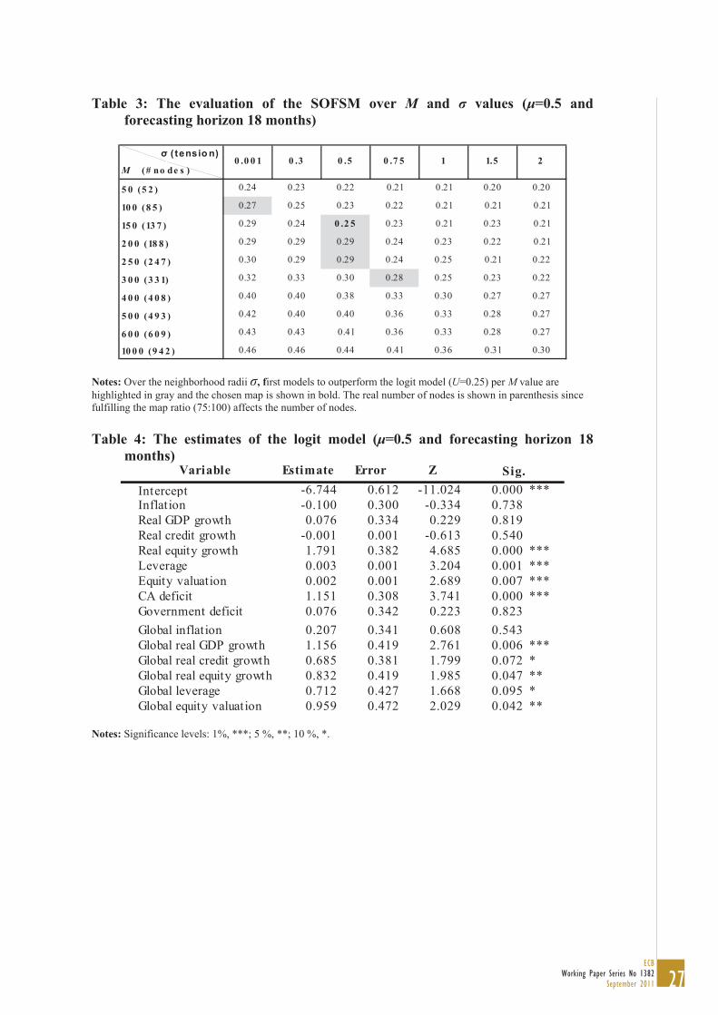
The evaluation results are shown in Table 2. For 1000,600,500,400,50M no model is chosen for analysis, as they never or always exceed the usefulness of the logit model (U=0.25). Finally, of the five highlighted models, we select the one with M=150 and 5.0 (shown in bold) for its interpretability and topological ordering.
(See Table 2) The chosen SOM has 137 nodes on an 11x13 grid and is trained with a tension of 0.5 Henceforth, this model is referred to as the Self-Organizing Financial Stability Map (SOFSM). Figures 1–3 present the two-dimensional grid of the SOFSM, the feature planes for the 14 indicators, and the feature planes for the class variables. The feature planes in Figure 3 show the real distribution of the classes on the SOFSM, while the lines that split the maps into four parts show the crisp clustering of the nodes based on all class variables (except the below explained PPC0). When maximizing the usefulness for policymakers with different preferences, Figure 4 shows how the map is classified into two parts, where the shaded area represents early warning nodes and the rest tranquil nodes. The feature plane PPC0, with a high frequency on the border between the post- and pre-crisis cluster, represents the co-occurrence of pre- and post-crisis periods. In this case, the cycle need not include the tranquil stage if a new pre-crisis period is entered directly after the previous event. Using the distribution of the class variables, the four clusters are labelled according to the stages of the financial stability cycle. The upper left cluster represents the pre-crisis cluster (Pre crisis), the lower left represents the crisis cluster (Crisis), the centre and lower-right cluster represents the post-crisis cluster (Post crisis) and the upper right represents the tranquil cluster (Tranquil). The main characteristics of the clusters can be derived from the feature planes in Figures 2–3. In contrast to EWSs using binary classification methods, such as discrete choice techniques, the SOFSM enables simultaneous assessment of the correlations with all four stages of the financial stability cycle. Thus, new models need not be derived for different forecasting horizons or definitions of the dependent variable. By assessing the feature planes of the SOFSM, the following strong correlations are found, for example. First, we can differentiate between early and late signs of a crisis by assessing differences within the pre-crisis cluster. The strongest early signs of a crisis (upper right part of the cluster) are high domestic and global real equity growth and 19 Due to no consensus on a single topology-preservation metric of the SOM projection, it is evaluated
following Kaski et al. (2000). The nodes im are projected into two- and three-dimensional spaces
using Sammon’s (1969) mapping, a non-linear mapping from a high-dimensional input space to a lower dimension. Topology preservation is defined to be adequate if the map is not twisted at any point and has only adjacent nodes as neighbours in Euclidean space. Interpretability is a subjective measure of the SOM visualization defined by the user.
16ECBWorking Paper Series No 1382September 2011
equity valuation, while most important late signs of a crisis (lower left part of the cluster) are domestic and global real GDP growth, and domestic real credit growth, leverage, budget surplus, and CA deficit. Second, the highest values of global leverage and real credit growth in the crisis cluster exemplify the fact that increases in some indicators may reflect a rise in financial stress only up to a specific threshold. Increases beyond that level are, in this case, more concurrent than preceding signals of a crisis. Similarly, budget deficits characterize the late post-crisis and early tranquil periods, while surpluses are signals of impending instabilities. The characteristics of the financial stability states are summarized in Table 3.
(See Table 3) The topological ordering of the SOFSM enables assessing, in terms of macro-financial conditions, neighbouring financial states of a particular position on the map. Transmission of financial contagion is often defined by other types of neighbourhood measures such as financial or trade linkages, proxies of financial shock propagation, equity market co-movement or geographical relations (see for example Dornbusch et al. (2000) and Pericoli and Sbracia (2003)). When assessing the SOFSM, the concept of neighborhood of a country represents the similarity of the current macro-financial conditions. Thus, a crisis in one position on the map indicates propagation of financial instabilities to adjacent locations. This type of representation may help in identifying events surpassing historical experience and the changing nature of crises.
(See Figure 1–4)
Evaluating the Self-Organizing Financial Stability Map A standard logit model is estimated using the same in-sample data as was used for the SOFSM. The estimates are reported in Table 4 and are later used for predicting out-of-sample data. The logit model’s in-sample and out-of-sample performance for the benchmark specifications ( 5.0 and C18) are shown in Table 5. For the benchmark models, the overall performance is similar between the SOFSM and the logit model. On the train set, the SOFSM performs slightly better than the logit model in terms of usefulness, recall positives, precision negatives and the AUC measure, while the logit model outperforms on the other measures. The classification of the models are of opposite nature, as the SOM issues more false alarms (FP rate=31%) than it misses crises (FN rate=19%), whereas the logit model misses more crises (31%) than it issues false alarms (19%). That explains also the difference in the overall accuracy, since the class sizes are unbalanced (around 20% crisis and 80% tranquil periods). The performance of the models on the test set differs, in general, similarly as the performance on the train set, except for the SOM having slightly higher overall accuracy. This is, in general, due to the higher share of crisis episodes in the out-of-sample dataset. We test the robustness of the SOFSM with respect to policymaker’s preferences ( 4.0 and 6.0 ), forecasting horizon (6, 12 and 24 months before a crisis) and thresholds (with the AUC measure). The results of the robustness tests are shown in Tables 6–7 and Figure 5. Table 6 shows the performance over different policymaker’s preferences, Table 7 over different forecasting horizons and Figure 5 and Tables 6–7
17ECB
Working Paper Series No 1382September 2011
over all possible thresholds. For a policymaker, who is less concerned about issuing false alarms ( 6.0 ), the performance of the models are similar, except for higher usefulness of the SOFSM compared to the logit model. This confirms that the SOM better detects the rare crisis occurrences. For a policymaker, who is less concerned about missing crises ( 4.0 ), the usefulness of the models is similar, but the nature of the prediction is reversed; the SOM issues less false alarms than it misses crises, whereas the logit model issues more false alarms than misses crises. Over different forecasting horizons, the in-sample performance is generally similar. However, the out-of-sample usefulness, with the exception of forecast horizon of 12 months (C12), is better for the SOFSM than for the logit model. Interestingly, the logit model fails to yield any usefulness (U=0.02) at a forecasting horizon of 6 months. Finally, the AUC measure, which summarizes the performance of a model over all thresholds, can be computed for all models by calculating the areas under the ROC curves, such as those shown in Figure 5 for the benchmark models ( 5.0 and C18). It is the only measure to consistently show superior performance for the SOFSM. A caution regarding the AUC measure is, however, that parts of the ROC curve that are not policy relevant are included in the computed area. When comparing usefulness for each pair of models, the SOFSM shows consistently equal or superior performance except for a single out-of-sample evaluation with a forecasting horizon of 12 months. To sum up, the SOM performs, in general, as well or better than a logit model in both classifying the in-sample data and in predicting out-of-sample the global financial crisis that started in 2007.
(See Table 4–7 and Figure 5)
4. Mapping the State of Financial Stability In this section, we use the SOFSM for mapping macro-financial conditions and the state of financial stability. We map samples of the panel dataset by showing cross-sectional and temporal data on the two-dimensional SOM grid. We also compute aggregates for groups of countries for exploring states of financial stability globally, in advanced economies and in emerging economies. Data points are mapped onto the grid by projecting them to their best-matching units (BMUs). Consecutive time-series data are linked with lines. Cross-sectional and temporal analysis on the SOFSM For a simultaneous temporal and comparative analysis, we map the state of financial stability based on the evolution of macro-financial conditions for the United States and the euro area in Figure 6. The data for both economies represent the first quarters of 2002 to 2010. Without a precise empirical treatment for accuracy, the map well recognizes for both countries the pre-crisis, crisis and post-crisis stages of the financial stability cycle by circulating around the map during the analyzed period. Interestingly, the euro area is located in the tranquil cluster in 2010Q1 (as well as in Q3 as is shown in Figure 7). This indicates that the aggregated macroprudential metrics for the euro area as a whole did not reflect the ongoing sovereign and banking crises in the euro area periphery. It also coincides with a relatively low FSI for the aggregate euro area. This can be explained by the weaknesses and financial stress in

18ECBWorking Paper Series No 1382September 2011
smaller economies being averaged out by improved macro-financial conditions in larger euro area economies, highlighting the importance of country-level analysis. Figure 7 represents a cross-section mapping of the state of financial stability for all countries in 2010Q3, which is the latest data point in the analysis. The countries are divided into three groups of financial stability states. The map indicates elevated risks in several emerging market economies (Mexico, Turkey, Argentina, Brazil, Taiwan, Malaysia and the Philippines), while most of the advanced economies are in the lower right corner of the map (post-crisis and tranquil cluster). Three countries (Singapore, South Africa and India) are located on the border of the tranquil and pre-crisis clusters, which is an indication of a possible future transition to the pre-crisis cluster. For this type of cross-sectional data, the topological ordering of the SOFSM enables assessing propagation of financial instabilities to adjacent macro-financial locations. When the SOFSM does not account for events surpassing historical data, as empirical models of non-stationary processes may do, this type of representation may help in identifying the changing nature of crises. For this cross section (Figure 7), a crisis in, say, Argentina and Brazil would as well indicate possible financial distress in neighbouring countries (Taiwan, Mexico and Turkey).
(See Figure 6–7) Exploring aggregate financial stability states on the SOFSM In this section, we map the financial stability states for three aggregates: the world, emerging market economies and advanced economies. We compute the state of financial stability for the aggregates by weighting the indicators for the countries in our sample using stock market capitalization to proxy their financial importance.20 These aggregates can, like any data point, be projected onto the map to their BMUs. Figure 8 shows the evolution of global macro-financial conditions in the first quarters of 2002 to 2010. The global state of financial stability enters the pre-crisis cluster in 2006Q1 and the crisis cluster in 2007Q1. It moves via the post-crisis cluster to the tranquil cluster in 2010Q1. This coincides with the global evolution of the financial stress index (FSI). The separation of the global aggregate into emerging market and advanced economies is shown in Figure 9. The mapping of the advanced economy aggregate is very similar to the one of the world aggregate, which is mainly a result of the small share of stock market capitalization of the emerging economies. Notably, the movements of the financial stability states of the emerging markets are also similar to those in the advanced economies, illustrating the global dimension of the current crisis. While the emerging market cycle moves around that of the advanced economies, it does not indicate significant differences in the timeline or strength of financial stress.
(See Figure 8–9)
20 The advanced economies are Australia, Denmark, euro area, Japan, New Zealand, Norway, Sweden, Switzerland, the United Kingdom, and the United States. The emerging market economies are Argentina, Brazil, China, Czech Republic, Hong Kong, Hungary, India, Indonesia, Malaysia, Mexico, the Philippines, Poland, Russia, Singapore, South Africa, Taiwan, Thailand and Turkey.

19ECB
Working Paper Series No 1382September 2011
5. Conclusions
This paper creates a Self-Organizing Financial Stability Map (SOFSM) for visualizing the sources of systemic risks and for predicting systemic financial crises. The SOFSM is a two-dimensional representation of a multidimensional financial stability space that allows disentangling the individual sources of vulnerabilities impacting on systemic risks. In addition, the model can be used to monitor macro-financial vulnerabilities by locating a country in the financial stability cycle: being it either in the pre-crisis, crisis, post-crisis or tranquil state. Our results indicate the SOFSM performs as well or better than a logit model in classifying in-sample data and predicting the global financial crisis that started in 2007. We test the robustness of the SOFSM by varying the thresholds of the models, the policymaker’s preferences, and the forecasting horizon.

20ECBWorking Paper Series No 1382September 2011
Annex: The SOM Algorithm This description of the SOM algorithm follows that in Sarlin (2011). This study uses the Viscovery SOMine 5.1 package.21 In addition to an easily interpretable visual representation and interaction features, it attempts to reduce computational cost by some extensions to the basic SOM. It employs the batch training algorithm, and thus processes data in batches instead of sequences. Important advantages of the batch algorithm are the reduction of computational cost and reproducible results (given the same initialization). The training process starts with initialization of the reference vectors set to the direction of the two principal components of the input data. The principal component initialization not only further reduces computational cost and enables reproducible results, but is also shown to be important for convergence when using the batch SOM (Forte et al., 2002). Following Kohonen (2001), this is done in three steps:
1. Determine two eigenvectors, v1 and v2, with the largest eigenvalues from the covariance matrix of all data .
2. Let v1 and v2 span a two-dimensional linear subspace and fit a rectangular array along it, where the two dimensions are the eigenvectors and the center coincides with the mean of . Hence, the direction of the long side is parallel to the longest eigenvector v1 with a length of 80% of the length of v1. The short side is parallel to v2 with a length of 80% of the length of v2.
3. Identify the initial value of the reference vectors mi(0) with the array points, where the corners of the rectangle are 21 4.04.0 vv .
Following the initialization, the batch training algorithm operates a specified number of iterations 1,2,…,t in two steps. In the first step, each input data vector x is assigned to the best-matching unit (BMU) mc:
)(min)( tmxtmx iic . (1)
We employ a semi-supervised version of the SOM by also including class information when determining the BMU. In the second step, each reference vector im (where i=1,2,…,M) is adjusted using the batch update formula:
N
jjic
N
jjjic
i
th
xthtm
1)(
1)(
)(
)()1( (2)
21 There are several other implementations of the SOM. The seminal packages – SOM_PAK, SOM Toolbox for Matlab, Nenet, etc – are not regularly updated or adapted to their environment. Out of the newer implementations, Viscovery SOMine provides the needed techniques for interactive exploratory analysis (Moehrmann et al., 2011). For a thorough discussion of SOM software and the implementation in Viscovery SOMine, see Deboeck (1998a; 1998b).

21ECB
Working Paper Series No 1382September 2011
where index j indicates the input data vectors that belong to node c, and N is the number of the data vectors. The neighbourhood function 1,0)( jich is defined as the following Gaussian function:
,)(2
exp 2
2
)( trr
h icjic (3)
where 2
ic rr is the squared Euclidean distance between the coordinates of the reference vectors mc and mi on the two-dimensional grid, and the radius of the neighbourhood )(t is a monotonically decreasing function of time t. The radius of the neighbourhood begins as half the diagonal of the grid size ( 2/)( 222 YX ), and goes monotonically towards the specified tension value 2,0)(t . Second-level clustering is done using an agglomerative hierarchical clustering. The following modified Ward’s (1963) criterion is used as a basis for measuring the distance between two candidate clusters:
,otherwise
adjacent are and if2 lkccnn
nnd lk
lk
lk
kl (4)
where k and l represent two clusters, kn and ln the number of data points in the
clusters k and l, and 2lk cc the squared Euclidean distance between the cluster
centres of clusters k and l. The Ward clustering is modified only to merge clusters with other topologically neighbouring clusters by defining the distance between non-adjacent clusters as infinitely large. The algorithm starts with each node as its own cluster and merges nodes for all possible numbers of clusters using the minimum Ward distance (1,2,…,M).

22ECBWorking Paper Series No 1382September 2011
References Alessi, L., Detken, C., 2011. Quasi real time early warning indicators for costly asset
price boom/bust cycles: A role for global liquidity. European Journal of Political Economy 27(3), 520–533.
Arciniegas Rueda, I.E., Arciniegas, F., 2009. SOM-based data analysis of speculative
attacks’ real effects. Intelligent Data Analysis 13(2), 261–300. Back, B., Sere, K., Vanharanta, H., 1998. Managing Complexity in Large Data Bases
using Self-Organizing Maps. Accounting, Management and Information Technologies 8(4), 191–210.
Balakrishnan, R., Danninger, S., Elekdag, S., Tytell, I., 2009. The Transmission of
Financial Stress from Advanced to Emerging Economies. IMF Working Paper, WP/09/133.
Berg, A., Borensztein, E., Pattillo, C., 2005. Assessing early warning systems: How
have they worked in practice?. IMF Staff Papers 52, 462–502. Berg, A., Pattillo, C., 1999. Predicting currency crises – the indicators approach and
an alternative. Journal of International Money and Finance 18, 561–586. Borio, C., Lowe, P., 2002. Asset Prices, Financial and Monetary Stability: Exploring
the Nexus. BIS Working Papers, No. 114. Borio, C., Lowe, P., 2004. Securing Sustainable Price Stability: Should Credit Come
Back from the Wilderness?. BIS Working Papers, No. 157. Bussière, M., Fratzscher, M., 2006. Towards a new early warning system of financial
crises. Journal of International Money and Finance 25(6), 953–973. Cardarelli, R., Elekdag, S., Lall, S., 2011. Financial stress and economic contractions.
Journal of Financial Stability 7(2), 78–97. Cox, T.F., Cox, M.A.A., 2001. Multidimensional Scaling. Chapman & Hall/CRC,
Florida. Dattels, P., McCaughrin, R., Miyajim, K., Puig, J., 2010. Can you Map Global
Financial Stability?. IMF Working Paper, WP/10/145. Deboeck, G., 1998a. Software Tools for Self-Organizing Map, in: Deboeck, G.,
Kohonen, T., (Eds.), Visual Explorations in Finance with Self-Organizing Maps, Springer-Verlag, Berlin, pp. 179–194.
Deboeck, G., 1998b. “Best practices in data mining using self-organizing maps, in:
Deboeck, G., Kohonen, T., (Eds.), Visual Explorations in Finance with Self-Organizing Maps, Springer-Verlag, Berlin, pp. 201–229.
Demirgüç-Kunt, A., Detragiache, E., 2000. Monitoring Banking Sector Fragility. A Multivariate Logit. World Bank Economic Review 14(2), 287–307.

23ECB
Working Paper Series No 1382September 2011
Demyanyk, Y.S., Hasan, I., 2010. Financial crises and bank failures: a review of prediction methods. Omega 38(5), 315–324.
Dornbusch, R., Park, Y.C., Claessens, S., 2000. Contagion: How it Spreads and How
it can be Stopped. World Bank Research Observer 15, 177–197. Eklund, T., Back, B., Vanharanta, H., Visa, A., 2000. Evaluating a SOM-based
financial benchmarking tool. Journal of Emerging Technologies in Accounting 5(1), 109–127.
Illing, M., Liu, Y., 2006. Measuring financial stress in a developed country: An
application to Canada. Journal of Financial Stability 2(3), 243–65. Fioramanti, M., 2008. Predicting sovereign debt crises using artificial neural
networks: a comparative approach. Journal of Financial Stability 4(2), 149–164. Forte, J.C., Letrémy, P., Cottrell, M., 2002. Advantages and drawbacks of the Batch
Kohonen algorithm, in: Verleysen, M., (Ed.), Proceedings of the 10th European Symposium on Neural Networks, Springer-Verlag, Berlin, pp. 223–230.
Fuertes, A.M., Kalotychou, E., 2006. Early Warning System for Sovereign Debt
Crisis: the role of heterogeneity. Computational Statistics and Data Analysis 5, 1420–1441.
Hakkio, C.S., Keeton, W.R., 2009. Financial Stress: What is it, How can it be
measured and Why does it matter?. Federal Reserve Bank of Kansas City Economic Review, Second Quarter 2009, 5–50.
Kaminsky, G., Lizondo, S., Reinhart, C., 1998. Leading Indicators of Currency
Crises. IMF Staff Papers 45(1), 1–48. Kaski, S., Venna, J., Kohonen, T., 2000. Coloring that reveals cluster structures in
multivariate data. Australian Journal of Intelligent Information Processing Systems 6, 82–88.
Kindleberger, C., 1996. Maniacs, Panics, and Crashes. Cambridge University Press,
Cambridge. Kohonen, T., 1982. Self-organized formation of topologically correct feature maps.
Biological Cybernetics 66, 59–69. Kohonen, T., 1982. Self-Organizing Maps, 3rd edition. Springer-Verlag, Berlin. Lo Duca, M., Peltonen, T.A., 2011. Macro-Financial Vulnerabilities and Future
Financial Stress – Assessing Systemic Risks and Predicting Systemic Events. ECB Working Paper, No. 1311.
Marghescu, D., 2007. Multidimensional Data Visualization Techniques for Exploring Financial Performance Data, in: Proceedings of 13th Americas Conference on Information Systems, Keystone, Colorado, USA.

24ECBWorking Paper Series No 1382September 2011
Matthews, B.W., 1975. Comparison of the predicted and observed secondary structure of T4 phage lysozyme. Biochimica et Biophysica Acta (BBA) – Protein Structure 405(2), 442–45.
Minsky, H., 1982. Can “it” Happen Again?: Essays on Instability and Finance. M.E.
Sharpe, Armonk, N.Y. Moehrmann, J., Burkovski, A., Baranovskiy, E., Heinze, G.A., Rapoport, A.,
Heideman, G., 2011. A Discussion on Visual Interactive Data Exploration Using Self-Organizing Maps, in: Laaksonen, J., Honkela, T., (Eds.), Proceedings of the 8th International Workshop on Self-Organizing Maps, Springer-Verlag, Berlin, pp. 178–187.
Peltonen, T.A., 2006. Are emerging market currency crises predictable? A test. ECB
Working Paper, No. 571. Pericoli, M., Sbracia, M., 2003. A Primer on Financial Contagion. Journal of
Economic Surveys 17, 571–608. Pöllä, M., Honkela, T., Kohonen, T., 2009. Bibliography of Self-Organizing Map
(SOM) Papers: 2002-2005 Addendum. TKK Reports in Information and Computer Science, Helsinki University of Technology, Report TKK-ICS-R24.
Resta, M., 2009. Early Warning Systems: an approach via Self Organizing Maps with
applications to emergent markets, in: Apolloni, B., Bassis, S., Marinaro, M. (Eds.), Proceedings of the 18th Italian Workshop on Neural Networks, IOS Press, Amsterdam, pp. 176–184.
Sammon Jr., J.W., 1969. A Non-Linear Mapping for Data Structure Analysis. IEEE
Transactions on Computers 18(5), 401–409. Sarlin, P., 2011. Sovereign Debt Monitor: A Visual Self-Organizing Maps Approach,
in: Proceedings of the IEEE Symposium on Computational Intelligence for Financial Engineering & Economics, IEEE Press, Paris, pp. 357–364.
Sarlin, P., Marghescu, D., 2011. Visual Predictions of Currency Crises using Self-
Organizing Maps. Intelligent Systems in Accounting, Finance and Management 18(1), 15–38.
Ward Jr., J.H., 1963. Hierarchical grouping to optimize an objective function. Journal
of the American Statistical Association 58, 236–244. Vesanto, J., Alhoniemi, E., 2000. Clustering of the self-organizing map. IEEE
Transactions on Neural Networks 11(3), 586–600.
22
Vesanto, J., Sulkava, M., Hollmén, J., 2003. On the decomposition of the self-organizing map distortion measure, in: Proceedings of the Workshop on Self-Organizing Maps (WSOM'03), Springer-Verlag, Berlin, pp. 11–16.
25ECB
Working Paper Series No 1382September 2011
Tab
le 1
: Sta
tistic
al p
rope
rtie
s of t
he d
atas
et
Type
Var
iabl
eA
bbre
viat
ion
Mea
nSD
Min
.M
ax.
Skew
.K
urt.
KSL
AD
Dom
estic
Infla
tiona
Infla
tion
0.89
5.17
-10.
1542
.53
4.80
26.7
20.
29*
263.
90*
Dom
estic
Real
GD
PbRe
al G
DP
grow
th3.
733.
76-1
7.54
14.1
3-0
.86
3.16
0.06
*11
.34*
Dom
estic
Real
cre
dit t
o pr
ivat
e se
ctor
to G
DPb
Real
cre
dit g
row
th23
4.07
4724
.00
-69.
4210
1870
.34
20.7
642
9.59
0.51
*In
f*D
omes
ticRe
al e
quity
pric
esb
Real
equ
ity g
row
th5.
9333
.01
-84.
4025
7.04
0.99
4.31
0.05
*7.
28*
Dom
estic
Cred
it to
priv
ate
sect
or to
GD
PaLe
vera
ge3.
4851
.64
-62.
7816
73.0
422
.76
673.
350.
29*
Inf*
Dom
estic
Stoc
k m
arke
t cap
italis
atio
n to
GD
PaEq
uity
val
uatio
n3.
9028
.32
-62.
7920
1.55
0.77
2.41
0.03
*3.
86*
Dom
estic
Curre
nt a
ccou
nt d
efic
it to
GD
PcCA
def
icit
-0.0
20.
07-0
.27
0.10
-0.9
80.
730.
09*
33.1
2*D
omes
ticGo
vern
men
t def
icit
to G
DPc
Gove
rnm
ent d
efic
it0.
010.
05-0
.19
0.22
-1.0
93.
460.
09*
35.9
0*Gl
obal
Infla
tiona
Glob
al in
flatio
n0.
030.
64-1
.33
2.29
0.71
1.28
0.08
*12
.12*
Glob
alRe
al G
DPb
Glob
al re
al G
DP
grow
th1.
841.
59-6
.34
4.09
-3.0
211
.74
0.20
*12
2.16
*Gl
obal
Real
cre
dit t
o pr
ivat
e se
ctor
to G
DPb
Glob
al re
al c
redi
t gro
wth
3.87
1.68
-0.2
37.
20-0
.21
-0.3
10.
07*
8.82
*Gl
obal
Real
equ
ity p
rices
bGl
obal
real
equ
ity g
row
th2.
3119
.08
-40.
6237
.77
-0.5
7-0
.68
0.15
*41
.90*
Glob
alCr
edit
to p
rivat
e se
ctor
to G
DPa
Glob
al le
vera
ge1.
152.
79-2
.79
11.2
11.
843.
400.
22*
105.
26*
Glob
alSt
ock
mar
ket c
apita
lisat
ion
to G
DPa
Glob
al e
quity
val
uatio
n0.
8917
.41
-40.
5427
.46
-0.5
0-0
.43
0.09
*19
.11*
N
otes
:Tra
nsfo
rmat
ions
: a , dev
iatio
n fr
om tr
end;
b , ann
ual c
hang
e; c , l
evel
. KSL
: Lill
iefo
rs' a
dapt
ion
of th
e K
olm
ogor
ov-S
mirn
ov n
orm
ality
test
. AD
: the
sta
ndar
d A
nder
son-
Dar
ling
norm
ality
te
st. S
igni
fican
ce le
vels
: 1%
, *.

26ECBWorking Paper Series No 1382September 2011
Tab
le 2
: Cha
ract
eris
tics o
f the
fina
ncia
l sta
bilit
y st
ates
Var
iabl
e
Cen
tre
R
ange
Cen
tre
R
ange
Cen
tre
R
ange
Cen
tre
R
ange
Infla
tion
0.49
[0.2
2,0.
66]
0.55
[0.3
0,0.
69]
0.59
[0.2
6,0.
76]
0.37
[0.1
7,0.
68]
Rea
l GD
P gr
owth
0.67
[0.4
0,0.
80]
0.48
[0.1
4,0.
83]
0.34
[0.2
5,0.
50]
0.53
[0.3
0,0.
72]
Rea
l cre
dit g
row
th0.
66[0
.28,
0.85
]0.
55[0
.35,
0.82
]0.
39[0
.18,
0.68
]0.
43[0
.21,
0.75
]
Rea
l equ
ity g
row
th0.
68[0
.41,
0.85
]0.
28[0
.16,
0.58
]0.
39[0
.23,
0.80
]0.
61[0
.40,
0.74
]
Leve
rage
0.63
[0.3
1,0.
80]
0.59
[0.3
7,0.
81]
0.52
[0.2
3,0.
83]
0.29
[0.1
8,0.
51]
Equi
ty v
alua
tion
0.73
[0.6
2,0.
80]
0.55
[0.2
7,0.
81]
0.33
[0.1
7,0.
66]
0.45
[0.3
0,0.
63]
CA
def
icit
0.58
[0.3
0,0.
78]
0.54
[0.2
6,0.
80]
0.48
[0.2
5,0.
77]
0.41
[0.1
9,0.
66]
Gov
ernm
ent d
efic
it0.
38[0
.19,
0.74
]0.
45[0
.22,
0.62
]0.
53[0
.32,
0.85
]0.
61[0
.26,
0.85
]
Glo
bal i
nfla
tion
0.33
[0.0
8 ,0.
61]
0.61
[0.3
4,0.
76]
0.46
[0.2
0,0.
79]
0.63
[0.1
1,0.
90]
Glo
bal r
eal G
DP
grow
th0.
67[0
.54,
0.74
]0.
67[0
.30,
0.86
]0.
29[0
.13,
0.69
]0.
45[0
.13,
0.71
]
Glo
bal r
eal c
redi
t gro
wth
0.55
[0.2
8,0.
77]
0.86
[0.6
1,0.
92]
0.37
[0.1
6,0.
67]
0.33
[0.1
5,0.
52]
Glo
bal r
eal e
quity
gro
wth
0.72
[0.4
7 ,0.
80]
0.4
[0.2
3,0.
63]
0.34
[0.1
1,0.
79]
0.54
[0.2
0,0.
73]
Glo
bal l
ever
age
0.35
[0.1
8,0.
60]
0.79
[0.5
7,0.
91]
0.58
[0.1
7,0.
77]
0.33
[0.1
6,0.
73]
Glo
bal e
quity
val
uatio
n0.
67[0
.48,
0.82
]0.
81[0
.54,
0.91
]0.
36[0
.14,
0.76
]0.
27[0
.19,
0.55
]
Pre
cris
isC
risi
sPo
st c
risi
sT
ranq
uil
N
otes
:Col
umns
repr
esen
t cha
ract
eris
tics (
clus
ter c
entre
and
rang
e) o
f the
fina
ncia
l sta
bilit
y st
ates
on
the
SOFS
M a
nd ro
ws r
epre
sent
indi
cato
rs. S
ince
dat
a ar
e tra
nsfo
rmed
to c
ount
ry-s
peci
fic
perc
entil
es, t
he su
mm
ary
stat
istic
s are
com
para
ble
acro
ss in
dica
tors
and
clu
ster
s.
27ECB
Working Paper Series No 1382September 2011
Table 3: The evaluation of the SOFSM over M and values ( =0.5 and forecasting horizon 18 months)
( tensio n)
M (# no de s )
5 0 (5 2 ) 0.24 0.23 0.22 0.21 0.21 0.20 0.20
10 0 (8 5 ) 0.27 0.25 0.23 0.22 0.21 0.21 0.21
15 0 (13 7 ) 0.29 0.24 0 .2 5 0.23 0.21 0.23 0.21
2 0 0 (18 8 ) 0.29 0.29 0.29 0.24 0.23 0.22 0.21
2 5 0 (2 4 7 ) 0.30 0.29 0.29 0.24 0.25 0.21 0.22
3 0 0 (3 3 1) 0.32 0.33 0.30 0.28 0.25 0.23 0.22
4 0 0 (4 0 8 ) 0.40 0.40 0.38 0.33 0.30 0.27 0.27
5 0 0 (4 9 3 ) 0.42 0.40 0.40 0.36 0.33 0.28 0.27
6 0 0 (6 0 9 ) 0.43 0.43 0.41 0.36 0.33 0.28 0.27
10 0 0 (9 4 2 ) 0.46 0.46 0.44 0.41 0.36 0.31 0.30
20 .0 0 1 0 .3 0 .5 0 .7 5 1 1.5
Notes: Over the neighborhood radii , first models to outperform the logit model (U=0.25) per M value are highlighted in gray and the chosen map is shown in bold. The real number of nodes is shown in parenthesis since fulfilling the map ratio (75:100) affects the number of nodes.
Table 4: The estimates of the logit model ( =0.5 and forecasting horizon 18 months)
Variable Estimate Error ZIntercept -6.744 0.612 -11.024 0.000 ***Inflation -0.100 0.300 -0.334 0.738Real GDP growth 0.076 0.334 0.229 0.819Real credit growth -0.001 0.001 -0.613 0.540Real equity growth 1.791 0.382 4.685 0.000 ***Leverage 0.003 0.001 3.204 0.001 ***Equity valuation 0.002 0.001 2.689 0.007 ***CA deficit 1.151 0.308 3.741 0.000 ***Government deficit 0.076 0.342 0.223 0.823Global inflation 0.207 0.341 0.608 0.543Global real GDP growth 1.156 0.419 2.761 0.006 ***Global real credit growth 0.685 0.381 1.799 0.072 *Global real equity growth 0.832 0.419 1.985 0.047 **Global leverage 0.712 0.427 1.668 0.095 *Global equity valuation 0.959 0.472 2.029 0.042 **
Sig.
Notes: Significance levels: 1%, ***; 5 %, **; 10 %, *.

28ECBWorking Paper Series No 1382September 2011
Tab
le 5
: Per
form
ance
of t
he b
ench
mar
k m
odel
s on
in-s
ampl
e an
d ou
t-of
-sam
ple
data
(=0
.5 a
nd fo
reca
stin
g ho
rizo
n 18
mon
ths)
.
Mod
elD
ata
set
Thre
shol
dPr
ecis
ion
Rec
all
Prec
isio
nR
ecal
lA
UC
MC
CLo
git
Tra
in0.
7216
219
083
073
0.46
0.69
0.92
0.81
0.79
0.25
0.81
0.44
SOM
Tra
in0.
6019
031
470
645
0.38
0.81
0.94
0.69
0.71
0.25
0.83
0.40
Logi
tT
est
0.72
7757
249
930.
570.
450.
730.
810.
680.
130.
720.
28SO
MT
est
0.60
112
8921
758
0.56
0.66
0.79
0.71
0.69
0.18
0.75
0.36
Neg
ativ
esA
ccur
acy
UTP
FPTN
FNPo
siti
ves
N
otes
: The
tabl
e re
ports
resu
lts fo
r the
logi
t and
SO
FSM
on
the
train
and
test
dat
a se
ts a
nd th
e op
timal
thre
shol
d. T
he th
resh
olds
are
cho
sen
to m
axim
ize
usef
ulne
ss w
ith
=0.5
and
fore
cast
ing
horiz
on 6
qua
rters
. The
Tab
le a
lso
repo
rts in
col
umns
the
follo
win
g m
easu
res t
o as
sess
the
perf
orm
ance
of t
he m
odel
s: T
P =
True
pos
itive
s, FP
= F
alse
pos
itive
s, TN
= Tr
ue n
egat
ives
, FN
=
Fals
e ne
gativ
es, P
reci
sion
pos
itive
s = T
P/(T
P+FP
), R
ecal
l pos
itive
s = T
P/(T
P+FN
), Pr
ecisi
on n
egat
ives
= T
N/(T
N+F
N),
Rec
all n
egat
ives
= T
N/(T
N+F
P), A
ccur
acy
= (T
P+TN
)/(TP
+TN
+FP+
FN),
U =
Use
fuln
ess (
see
form
ulae
6 a
nd 7
), A
UC
= a
rea
unde
r the
RO
C c
urve
(TP
rate
to F
P ra
te, s
ee S
ectio
n 2
and
Figu
re 4
) and
MC
C =
(TP*
TN-
FP*F
N)/
((TP
+FP)
(TP+
FN)(
TN+F
P)(T
N+F
N))
.
Tab
le 6
: Rob
ustn
ess t
ests
on
in-s
ampl
e an
d ou
t-of
-sam
ple
data
for
diff
eren
t μ v
alue
s (fo
reca
stin
g ho
rizo
n 18
mon
ths)
Mod
elD
ata
set
Thre
shol
dPr
ecis
ion
Rec
all
Prec
isio
nR
ecal
lA
UC
MC
CLo
git
Tra
in0.
40.
7216
219
083
073
0.46
0.69
0.92
0.81
0.79
0.16
0.81
0.44
SOM
Tra
in0.
40.
7515
316
685
482
0.48
0.65
0.91
0.84
0.80
0.16
0.83
0.44
Logi
tT
rain
0.5
0.72
162
190
830
730.
460.
690.
920.
810.
790.
250.
810.
44SO
MT
rain
0.5
0.60
190
314
706
450.
380.
810.
940.
690.
710.
250.
830.
40Lo
git
Tra
in0.
60.
5419
738
163
938
0.34
0.84
0.94
0.63
0.67
0.15
0.81
0.36
SOM
Tra
in0.
60.
5021
441
960
121
0.34
0.91
0.97
0.59
0.65
0.18
0.83
0.39
Logi
tT
est
0.4
0.72
7757
249
930.
570.
450.
730.
810.
680.
070.
720.
28SO
MT
est
0.4
0.75
7656
250
940.
580.
450.
730.
820.
680.
070.
750.
28Lo
git
Tes
t0.
50.
7277
5724
993
0.57
0.45
0.73
0.81
0.68
0.13
0.72
0.28
SOM
Tes
t0.
50.
6011
289
217
580.
560.
660.
790.
710.
690.
180.
750.
36Lo
git
Tes
t0.
60.
5411
010
919
760
0.50
0.65
0.77
0.64
0.64
0.05
0.72
0.28
SOM
Tes
t0.
60.
5013
410
919
736
0.55
0.79
0.85
0.64
0.70
0.13
0.75
0.41
Neg
ativ
esA
ccur
acy
UTP
FPTN
FNPo
siti
ves
N
otes
: See
the
note
s for
Tab
le 5
.

29ECB
Working Paper Series No 1382September 2011
Tab
le 7
: Rob
ustn
ess t
ests
on
in-s
ampl
e an
d ou
t-of
-sam
ple
data
for
diff
eren
t hor
izon
s (=0
.5)
Mod
elD
ata
set
Hor
izon
Thre
shol
dPr
ecis
ion
Rec
all
Prec
isio
nR
ecal
lA
UC
MC
CLo
git
Tra
inC6
0.72
7028
288
221
0.20
0.77
0.98
0.76
0.76
0.26
0.81
0.30
SOM
Tra
inC6
0.51
8853
063
43
0.14
0.97
1.00
0.54
0.58
0.26
0.83
0.27
Logi
tT
rain
C12
0.72
117
235
855
480.
330.
710.
950.
780.
770.
250.
800.
37SO
MT
rain
C12
0.69
123
267
823
420.
320.
750.
950.
760.
750.
250.
840.
37Lo
git
Tra
inC1
80.
7216
219
083
073
0.46
0.69
0.92
0.81
0.79
0.25
0.81
0.44
SOM
Tra
inC1
80.
6019
031
470
645
0.38
0.81
0.94
0.69
0.71
0.25
0.83
0.40
Logi
tT
rain
C24
0.58
242
286
673
540.
460.
820.
930.
700.
730.
260.
810.
45SO
MT
rain
C24
0.63
233
241
718
630.
490.
790.
920.
750.
760.
270.
850.
47Lo
git
Tes
tC6
0.72
1811
630
240
0.13
0.31
0.88
0.72
0.67
0.02
0.57
0.02
SOM
Tes
tC6
0.51
4720
521
311
0.19
0.81
0.95
0.51
0.55
0.16
0.65
0.21
Logi
tT
est
C12
0.72
4985
275
670.
370.
420.
800.
760.
680.
090.
640.
18SO
MT
est
C12
0.69
5110
225
865
0.33
0.44
0.80
0.72
0.65
0.08
0.68
0.14
Logi
tT
est
C18
0.72
7757
249
930.
570.
450.
730.
810.
680.
130.
720.
28SO
MT
est
C18
0.60
112
8921
758
0.56
0.66
0.79
0.71
0.69
0.18
0.75
0.36
Logi
tT
est
C24
0.58
132
6818
591
0.66
0.59
0.67
0.73
0.67
0.16
0.76
0.33
SOM
Tes
tC2
40.
6315
051
202
730.
750.
670.
730.
800.
740.
240.
800.
48
Neg
ativ
esA
ccur
acy
UTP
FPTN
FNPo
siti
ves
N
otes
: See
the
note
s for
Tab
le 5

30ECBWorking Paper Series No 1382September 2011
Figure 1: The two-dimensional grid of the SOFSM
Crisis
TranquilPre crisis
Post crisis
Notes: The figure displays the two-dimensional grid of the SOFSM, which enables a two-dimensional representation of the multidimensional financial stability space. The lines that separate the map into four parts are based on the distribution of the four underlying financial stability states and should only be interpreted as an aid in finding the states of the financial stability cycle, not as completely distinct clusters. The shades on the SOFSM show within a cluster the distance of each node to the centers of the financial stability states. For distributions of indicators and class variables on the SOFSM, see Figures 2–3.

31ECB
Working Paper Series No 1382September 2011
Figu
re 2
: The
feat
ure
plan
es fo
r th
e 14
indi
cato
rs a
nd th
e m
ain
clas
s var
iabl
es
Infla
tion
Pre
cris
is
Cri
sis
Post
cri
sisTr
anqu
il
0.17
0.29
0.41
0.52
0.64
0.76
Rea
l GD
P g
row
th
Pre
cris
is
Cri
sis
Post
cri
sisTr
anqu
il
0.14
0.27
0.41
0.55
0.69
0.83
Rea
l cre
dit g
row
th
Pre
cris
is
Cri
sis
Post
cri
sisTr
anqu
il
0.18
0.32
0.45
0.58
0.71
0.85
CA
def
icit
Pre
cris
is
Cri
sis
Post
cri
sisTr
anqu
il
0.19
0.31
0.43
0.55
0.68
0.80
Gov
ernm
ent d
efic
it
Pre
cris
is
Cri
sis
Post
cri
sisTr
anqu
il
0.19
0.32
0.46
0.59
0.72
0.86
Glo
bal i
nfla
tion
Pre
cris
is
Cri
sis
Post
cri
sisTr
anqu
il
0.08
0.25
0.41
0.57
0.73
0.90
Glo
bal l
ever
age
Pre
cris
is
Cri
sis
Post
cri
sisTr
anqu
il
0.16
0.31
0.46
0.61
0.76
0.91
Glo
bal e
quity
val
uatio
n
Pre
cris
is
Cri
sis
Post
cri
sisTr
anqu
il
0.14
0.30
0.45
0.60
0.75
0.91
Pre
-cris
is p
erio
ds
Pre
cris
is
Cri
sis
Post
cri
sisTr
anqu
il
0.01
0.14
0.27
0.39
0.52
0.65
Rea
l equ
ity g
row
th
Pre
cris
is
Cri
sis
Post
cri
sisTr
anqu
il
0.16
0.30
0.43
0.57
0.71
0.85
Leve
rage
Pre
cris
is
Cri
sis
Post
cri
sisTr
anqu
il
0.18
0.31
0.44
0.57
0.70
0.83
Equ
ity v
alua
tion
Pre
cris
is
Cri
sis
Post
cri
sisTr
anqu
il
0.17
0.30
0.43
0.55
0.68
0.81
Glo
bal r
eal G
DP
gro
wth
Pre
cris
is
Cri
sis
Post
cri
sisTr
anqu
il
0.13
0.28
0.42
0.57
0.71
0.86
Glo
bal r
eal c
redi
t gro
wth
Pre
cris
is
Cri
sis
Post
cri
sisTr
anqu
il
0.15
0.31
0.46
0.61
0.76
0.92
Glo
bal r
eal e
quity
gro
wth
Pre
cris
is
Cri
sis
Post
cri
sisTr
anqu
il
0.11
0.25
0.39
0.52
0.66
0.80
Cris
is p
erio
ds
Pre
cris
is
Cri
sis
Post
cri
sisTr
anqu
il
0.00
0.14
0.28
0.42
0.56
0.70
Pos
t-cris
is p
erio
ds
Pre
cris
is
Cri
sis
Post
cri
sisTr
anqu
il
0.06
0.18
0.29
0.40
0.52
0.63
Tran
quil
perio
ds
Pre
cris
is
Cri
sis
Post
cri
sisTr
anqu
il
0.02
0.18
0.34
0.50
0.66
0.82
N
otes
:The
feat
ure
plan
es a
re la
yers
of t
he S
OFS
M in
Fig
ure
1. W
hile
the
indi
cato
rs a
re d
efin
ed in
Tab
le 1
, the
four
mai
n cl
ass
varia
bles
are
Pre
cris
is (C
18),
Cris
is (C
0), P
ost c
risis
(P18
) and
Tr
anqu
il pe
riods
(T0)
. As
each
dat
a ro
w in
the
data
set
con
sist
s of
dat
a co
lum
ns fo
r 14
indi
cato
rs a
nd 4
mai
n cl
ass
varia
bles
, the
se fe
atur
e pl
anes
sho
w th
e di
strib
utio
n of
eac
h da
ta c
olum
n on
th
e gr
id. I
n th
e ca
se o
f bin
ary
clas
s var
iabl
es th
at ta
ke v
alue
s 1 a
nd 0
, hig
h va
lues
repr
esen
t a h
igh
prop
ortio
n of
dat
a in
diff
eren
t per
iods
(pre
-cris
is, c
risis
, pos
t-cris
is o
r tra
nqui
l per
iods
).

32ECBWorking Paper Series No 1382September 2011
Figure 3: Feature planes for all classes C24
Pre crisisTranquil
Crisis
Post crisis
0.01 0.26 0.50 0.75
C18
Pre crisisTranquil
Crisis
Post crisis
0.01 0.22 0.44 0.65
C12
Pre crisisTranquil
Crisis
Post crisis
0.00 0.18 0.35 0.53
C6
Pre crisisTranquil
Crisis
Post crisis
0.00 0.11 0.21 0.32
C0
Pre crisisTranquil
Crisis
Post crisis
0.00 0.23 0.47 0.70
P6
Pre crisisTranquil
Crisis
Post crisis
0.00 0.11 0.22 0.33
P12
Pre crisisTranquil
Crisis
Post crisis
0.01 0.18 0.35 0.52
P18
Pre crisisTranquil
Crisis
Post crisis
0.06 0.25 0.44 0.63
P24
Pre crisisTranquil
Crisis
Post crisis
0.13 0.32 0.50 0.68
T0
Pre crisisTranquil
Crisis
Post crisis
0.02 0.29 0.55 0.82
PPC0
Pre crisisTranquil
Crisis
Post crisis
0.00 0.09 0.18 0.27Notes: The figure shows the distributions of different pre- and post-crisis horizons in more detail. As in Figure 2, these are layers of the SOFSM in Figure 1. The feature planes C24, C18, C12, C6, P24, P18, P12 and P6 show the map distribution of class variables that represent 24, 18, 12 and 6 months before and after a crisis, respectively. While C0 and T0 show the distribution of crisis and tranquil periods, PPC0 represents the co-occurrence of pre- and post-crisis periods.
Figure 4: Early warning nodes for different policymakers’ preferences =0.4 =0.5 =0.6
Notes: In the figure, the shaded area on the SOFSM (same map as in Figure 1) represents the part of the map that is classified as early warning nodes when maximizing the policymakers’ preferences with three different parameter values (μ=0.4, μ=0.5 and μ=0.6) and a horizon of 18 months according to the evaluation framework.

33ECB
Working Paper Series No 1382September 2011
Figure 5: In-sample and out-of-sample Receiver Operating Characteristics (ROC) curves for SOFSM and logit models (with =0.5 and horizon 18 months)
0.0 0.5 1.0
0.0
0.5
1.0
In-sample
FP rate
TP ra
te
Logit SOFSM
0.0 0.5 1.0
0.0
0.5
1.0
Out-of-sample
FP rate
TP ra
te
Notes: The vertical and horizontal axes represent True Positives (TP) rate (TP / (TP + FN)) and False Positives (FP) rate (FP/(FP+TN)). The area under the ROC curve (AUC), given in Tables 5–7, measures the area below these curves.

34ECBWorking Paper Series No 1382September 2011
Figure 6: A mapping of the financial stability states of the United States and the euro area in 2002–2010
US2004-05
US2006
US 2007
US20022010
Euro2006
Euro2002 Euro
2010
Euro2007
Euro2008
US 2008-09
US2003
Euro 2009Euro
2003
Euro2004-05
Pre crisis
Crisis
Post crisis
Tranquil
Notes: The figure displays the two-dimensional grid of the SOFSM. The lines that separate the map into four parts are based on the distribution of the four underlying financial stability states. The shades on the SOFSM show within a cluster the distance of each node to the centers of the financial stability states. The data for both economies represent the first quarters of 2002–2010.

35ECB
Working Paper Series No 1382September 2011
Figure 7: A cross-sectional mapping of financial stability states for countries in the sample in 2010Q3
Taiwan
India
UK Indonesia
JapanThailand
Canada Russia Czech Republic
Poland
Norway
Hungary
ChinaHong KongSwitzerland
AustraliaNew Zealand
US
Denmark Euro area
Korea Sweden
Argentina Brazil
Mexico Turkey
MalaysiaPhilippines
SingaporeSouth Africa
Crisis
Post crisis
TranquilPre crisis
Notes: The figure displays the two-dimensional grid of the SOFSM. The lines that separate the map into four parts are based on the distribution of the four underlying financial stability states. The shades on the SOFSM show within a cluster the distance of each node to the centers of the financial stability states. The data for all economies represent the third quarter of 2010.
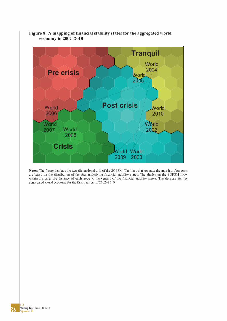
36ECBWorking Paper Series No 1382September 2011
Figure 8: A mapping of financial stability states for the aggregated world economy in 2002–2010
Crisis
Tranquil
Pre crisis
Post crisis
World2004
World 2005
World2006
World 2007
World 2002 World
2008
World2009
World 2003
World2010
Notes: The figure displays the two-dimensional grid of the SOFSM. The lines that separate the map into four parts are based on the distribution of the four underlying financial stability states. The shades on the SOFSM show within a cluster the distance of each node to the centers of the financial stability states. The data are for the aggregated world economy for the first quarters of 2002–2010.
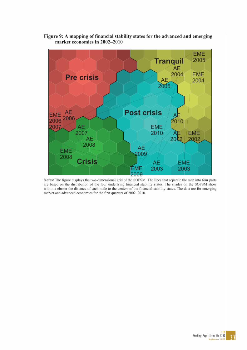
37ECB
Working Paper Series No 1382September 2011
Figure 9: A mapping of financial stability states for the advanced and emerging market economies in 2002–2010
Crisis
Pre crisis
Post crisis
EME 2005
AE2004 EME
2004AE2005
AE2006 AE
2010 AE
2007EME2010 AE
2002 EME 2002
EME2008
AE 2008
AE2003
EME2003
EME20062007
Tranquil
AE 2009
EME2009
Notes: The figure displays the two-dimensional grid of the SOFSM. The lines that separate the map into four parts are based on the distribution of the four underlying financial stability states. The shades on the SOFSM show within a cluster the distance of each node to the centers of the financial stability states. The data are for emerging market and advanced economies for the first quarters of 2002–2010.

Work ing PaPer Ser i e Sno 1118 / november 2009
DiScretionary FiScal PolicieS over the cycle
neW eviDence baSeD on the eScb DiSaggregateD aPProach
by Luca Agnello and Jacopo Cimadomo