Embed Size (px)
Citation preview
Macroeconomics
Cheng Wang
Department of Economics
Iowa State University
Spring, 2007
Part of this note is taken from Mankiw (2007).
1
Goals
• The first goal of this course is to acquaint you with fundamental
principles and methods of modern macroeconomic theories.
• The second goal of this course is to teach you how to use these
principles and methods to think about macroeconomic issues in
real life.
• The third goal, which is more specific, is that after this course,
you should be able to understand almost all the reports and
rebate related to macroeconomic data and policy in the Wall
Street Journal.
2
Chapter 1Introduction
1 What is Macroeconomics?
• Macroeconomics studies the economy as a whole. It tries to
explain how the economy as a whole works and seeks to find out
ways (design economic policies, institutions) to make it work
more efficiently.
• Microeconomics is the study of how individual economic agents
(workers, managers, students and professors, firms, universities)
make decisions (behave) and how these decision makers (their
behavior) interact in individual markets.
• (What’s the marketplace? e-market?)
3
2 A List of Macro and Micro Economic Questions
• What determines a country’s Real GDP (which measures the
total income of everyone in the economy, adjusted for price
changes)? What determines an economy’s growth path in the
long-run?
• How does a farmer set the price of corns? How does a firm decide
what to produce, and how much to produce? What determines
a firm’s dividend policy? Why do firms pay dividends? What
explains mergers and takeovers? Why are prices sticky? Why
do firms use stock options to compensate their managers? What
explains the Golden Parachute?
• What explains business fluctuations? what explains unemploy-
ment? What explains the great depression? What explains the
new economy? What explains the so-called globalization?
• How to reduce unemployment and business fluctuations? What
is the optimal size of the government deficit or surplus? How
does the Fed decide what kind of monetary policy to implement?
How does the federal reserve decide to cut or raise the interest
rate?
4
3 Why Macroeconomics?
Macroeconomics is important for anybody that must live a life in a
modern economic society.
You are a student. You probably want to know how the labor market
is going to be in two or three years. That has a lot to do with how
the macroeconomy is performing in two or three years, whether the
economy is going to keep growing or go into a new recession. That in
turn may have to do with the government’s macro policies, fiscal and
monetary policies. If for example the government thinks derflation is
still a threat to growth anfdit then follows an expansionary monetary
policy to fight. This might be good news for you. If the gobvernment
sees inflation rising and then follows a policy to tighten money supply,
the economy is likely to slow down and that can have a negative
effects on the labor market.
If you are an investor. I are sitting on a bunch of cash. To invest
in realstate or in stocks? It again depends on how you think the
macroeconomy is doing. If you think the macroeconmy is picking up
speed and so stocks are rising higher, whereas interest rates are likely
to increase to crash the realstate market, you probably want to buy
stocks.
Macroeconomics is important for each of us in a sense because wach
of us must live in the macroeconomy. Each o9f us is part of the
macroeconomy. Each of us must make decisions thayt depend on
how the economy as a whole is doing.
Likewise, business firms and institutions must also operate in the
5
macro economy. Macroeconomy is thus also essential for business
decision making.
For instance, suppose your firm is thinking about invest in a new
project. You must borrow to invest. You must then think about the
interest rate. Interest rates that are too high can make your project’s
NPV negative. You must then think how the central bank’s policy
is going to be. That’s macro. The interest rate isa a key macro
variable.
If your company wants to acquire a smaller competitor. That costs
cash. You must be careful. Where the macroeconomy is standing?
Is it going into a recession? If yes, you may want to conserve cash to
prepare for the forthcoming winter. If on the other hand the economy
is booming and future cash flows are expected to be higher then you
are in a very different position.
You work for the company’s human resources department. To hire
new workers now? That again requires you to judge how the economy
is a whole is doing, because the depend for your company’s product
depends on whether your customers are spending. Hiring and firing
are both costly.
You company is thinking about entering an exporting business. You
worry about the exchange rates and the government’s trade policies.
Macroeconomics again. If the domestic currency is appreciating,
that’s going to make it harder for you to sell in foreign markets.
Higher exchange rates make your product more expensive for for-
eigners.
6
4 How Do Economists Think?
• I want to make this course the first serious economics course
you are going to have.
• Serious in the sense that most material I teach will be based
on rigorous scientific treatments.
• Serious also in the sense that I am going to treat all of you in
this classroom as future economists. Starting this course, you
have to learn how to think like an economist.
• How does the economist approach a question he has in mind?
The answer is: He constructs and uses models.
• A model is a simplied version of reality. Reality is often highly
multi-dimensional and complex, a model leaves out details which
are not essential to the issue at hand.
A model is like a map that shows the connections of economic
variables that you are interested in.
A model is a like a lab which economists use to conduct thought
experiments. Each model is a tool that economists use for study-
ing a specific set of questions.
• For economists, models are often mathematical. Making models
mathematical has benefits which I will discuss as I proceed.
• How to construct models? What makes a good model? How
to use models? — One purpose of this course is teach you how
to construct a model, and then use it to derive answers to the
questions at hand.
7
5 The Model of Demand and Supply — A Review
• Suppose an economist wants to analyse what determines the
price of corns and the quantity of corns sold in the market. He
most likely would construct a model with three major compo-
nents: One component that describes the buyers’ behavior, the
second describing the sellers’ behavior, and the third describing
how the market functions (the market structure).
• He assumes that the buyers’ behavior can be summarized by the
demand function
Qd = D(P, Y ) (1)
where Qd denotes the aggregate quantity of corns demanded, D
is the “demand function”, P is the price of corns, and Y is the
economy’s total income (real GDP). The above equation simply
states that the aggregate demand for corns is determined by
the price at which corns are to be sold and the economy’s total
purchasing power.
• He then assumes that the sellers’ behavior can be summarized
by the following supply function
Qs = S(P, Pm) (2)
where Qs denotes the aggregate quantity of corns supplied, S is
the “supply function”, P is the price of corns, and Pm is the price
of materials involved the production of corns (i.e., Pm indicates
the cost of producing corns).
8
• The economist then makes an assumption about how the buyers
and sellers interact in the market. Specifically, he assumes
(1) If Qs > Qd, that is, if there is “excess supply”, then price
will fall.
(2) If Qs < Qd, that is, if there is “excess demand”, then price
will rise.
And thus the price is stable (when the market reaches an equilib-
rium) only when demand and supply are in balance (the market
clears):
Qs = Qd. (3)
The above equation shows how the market works: it sets the
price to equate demand and supply.
• To summarize, equation (1) states how the buyers behave, equa-
tion (2) describes how the sellers behave, equation (3) describes
how buyers and sellers interact.
• Figures 1-5,1-6
9
6 The Model of Demand and Supply – An Example
Suppose the demand function is
D(P, Y ) = 60 − 10P + 2Y.
Suppose the supply function is
S(P, Pm) = 60 + 5P − Pm.
Suppose it is given that Y = 10 and Pm = 10.
Question: What is the equilibrium price and what is the equilib-
rium quantity?
Well, the equilibrium price must equate demand and supply:
60 − 10P + 2Y = 60 + 5P − Pm.
Given Y = Pm = 10, we have
60 − 10P + 2 ∗ 10 = 60 + 5P − 10
which in turn implies 30 = 15P or
P = 2,
and the equilibrium quantity bought and sold is equal to
Q = 60 − 10P + 2Y = 60.
Classwork: What happen if Y falls from 10 to 5?
10
7 Exogenous and Endogenous Variables
• Models have two kinds of variables: endogenous variables and
exogenous variables.
• Exogenous variables are the variables that are determined out-
side the model, the variables that the model take as given, the
variables that the economist does not intend to use the model to
explain.
• Endogenous variables are the variables that the model tries to
explain, these are the variables that are to be determined inside
the model.
• The endogenous variables in the above model of demand and
supply are the price of corns and the quantity of corns exchanged.
• Models are built to show how changes in the model’s exogenous
variables affect its endogenous variables.
Readings: Mankiw: Chapter 1.
11
Chapter 2Macro Economic Variables
8 Gross Domestic Product (GDP)
• GDP is the total dollar value of all final goods and services pro-
duced in a country within a given period of time.
• GDP includes the value of goods produced, such as houses and
corns. It also includes the value of services, such as airplane
rides and the professors’ lectures. The output of each of these is
valued at its market price, and the values are added together to
get GDP.
• The level of GDP is computed every three months by the Bu-
reau of Economic Analysis (a part of the U.S. Department of
Commerence).
• In 1997, the GDP of the United States is about 8 trillion dollars.
In 1997 the US population is about 268 million. Thus in 1997
the per capita GDP (GDP per person) is roughly 30, 000 US
dollars.
12
9 Computing GDP
• Suppose the economy produces two types of goods, apples and
oranges. Then
GDP = Price of Apples times quanty of apples
+ Price of oranges times quantity of oranges
• Suppose the price of apples is 0.5 and the price of oranges is 1.0.
Suppose the economy produced 4 units of apples and 3 units of
oranges. Then
GDP = 0.5 ∗ 4 + 1.0 ∗ 3 = 5.00.
• Suppose the economy produces N types of goods, the price of
the ith type is Pi, and the quantity of the ith type good is Qi.
Then
GDP = P1 ∗Q1 + P2 ∗Q2 + ... + PN ∗QN .
13
10 Nominal versus Real GDP
• Prices of goods change over time. The value of final goods and
services measured at current prices is called Nominal GDP. The
value of goods and services measured using a set of constant
prices (base year prices, the base year can be for example 1992)
is called the Real GDP.
Suppose again the economy produces two types of goods, apples
and oranges. Suppose we choose 1998 as the base year. Then
Real GDP of 2002
= 1998 Price of Apples ∗ 2002 quanty of apples
+ 1998 Price of oranges ∗ 2002 price of oranges
and
Nominal GDP of 2002
= 2002 Price of Apples ∗ 2002 quanty of apples
+ 2002 Price of oranges ∗ 2002 price of oranges
14
11 Some Notes
• GDP measures the value of currently produced goods and ser-
vices. Used goods are not included. The sale of used cars, for
example, are not included in GDP.
• The sale of intermediate goods are not included in GDP. GDP
includes only final goods and services.
For example, suppose a cattle rancher sells one unit of meart
to McDonald’s for 0.5 dollars, and then McDonald’s sells you a
hamburger for 1.50 dollars. Should GDP include both the meat
and the hamburger (a total of 2 dollars) or just the hamburger
(1.5 dollars)?
• Inventories are often included in GDP.
15
12 National Income Accounting
• Goods and services produced by the economy are ultimately pur-
chased by consumers and other agents who spend money to buy
them. A useful division of GDP according to alternative uses of
the economy’s output is the following:
Y = C + I + G + NX
where Y stands for GDP, C is consumption, I is investment, G
is government purchases, and NX is net exports.
16
• Consumption consists of goods and services bought by households
or consumers.
Durable goods: goods that last a long time, such as cars and
TYs.
Nondurable goods: goods that last a short time, such as food
and clothing.
Services: such as haircuts and airplane rides.
• Investment consists of good bought for future use. Investment
can also be divided into three categories.
Business fixed investment: new machinery and equipment bought
by firms.
Residential fixed investment: new houses bought by households.
Inventory investment: increase in firms’ inventories.
• Government Purchases are the goods and services bought by fed-
eral, state and local governments. This includes military equip-
ment, highways and bridges, and the services of government em-
ployees.
• Net Exports are the goods and services purchased by foreigners.
17
13 The Components of GDP
• Table 2.1.
• The Increasing role of services:
In 1992, the sevice sector in the US accounts for 72 percent of
its GDP (in Germany it is 57 percent) and emplyed 76 percent
of its labor force.
Meanwhile, the share of manufacturing has fallen in all the big
economies. In 1992, it accounts for only 23 percent of America’s
GDP and even smaller 18 percent of jobs. In Britain and Canada
manufacturing has also tumbled to less than 20 percent. Even in
Japan and Germany, the strongholds of manufacturing, services
is no more than 30 percent of GDP.
Services are also the fastest growing part of international trade,
accounting for 20 percent of total world trade and 30 percent of
American exports.
• The services Sector:
Legal services, business services (consulting), health, hotels, ed-
ucation, financial services, transport and communications.
18
14 Other Measures of Income
• GNP, gross national product, measures total income earned by
nationals.
GNP is equal to GDP plus total income earned by US nationals
in other countries minus income earned domestically by foreign
nationals.
• NNP, net national product, is GNP net of the depreciation of
capital.
Depreciation, the consumption of fixed capital, is the amount
of the economy’s capital stock that wears out during the year.
Depreciation equals 10 percent of GNP each year.
Because the depreciation of capital is a cost of producing the
output of the economy, subtracting it from GNP shows the net
result of economic activity.
• National Income is NNP minus Indirect Business Taxes (sales
taxes). NNP measures how much everyone in the economy has
earned after the indirect taxes.
Indirect business taxes are the difference between the price the
consumers pay and the the price the firm receives.
Important: employee compensation accounts for 70 percent of
national income, corporate profits 12 percent.
• Disposable Personal Income is the amount households and non-
corporate businesses have available after satisfying their tax obli-
gations to the government.
19
15 The GDP Deflator
Different goods and services have different prices and they change
over time and relative to each other. Economists want to sum-
merize the Overall level of prices in the economy in one number.
One index that does that is the GDP Deflator, also called the
implicit price deflator for GDP.
GDP Deflator =Nominal GDP
Real GDP.
or
Nominal GDP = Real GDP ×GDP Deflator
Thus the definition of the GDPdeflator separates nominal GDP
into two parts: the part that measures quantities (real GDP)
and the other that measures prices (the GDP deflator).
Here, nominal GDP measures the current dollar value of the
output of the economy. Real GDP measures the economy’s cur-
rent output valued at constant (base-year) prices. The GDP
deflator merasures the price of output (or the overall level of
current prices) relative to its price in the base year.
20
To better understand this, consider an economy with only one
good, corns. Let P be the current price of corns. Let Q be the
quantity of corns the ecconomy produces currently. Let Pbas be
the price of corns in some base year. Then Nominal GDP is
P ∗Q and real GDP is Pbas ∗Q and
GDP Deflator =P
Pbas
which is just the price of corns in the current year relative to the
price of corns in the base year.
Note: Suppose the economy produces two goods, or three goods,
do you know how compute the GDP deflator?
21
16 The Consumer Price Index
The Consumer Price Index (CPI) is the most commonly used
measure of the economy’s overall levcl of prices.
The aim of CPI is to measure in a single index the cost of liv-
ing. It focuses on the prices of goods and services that typical
consumers buy (or the goods and services included in a typi-
cal consumer’s basket), not the prices of all goods and services
produced in the whole economy.
Suppose a typical consumer buys 5 apples and 2 oranges every
month. Suppose 1992 is chosen to be the base year. Then
CPI =5 ∗ current price of apples + 2 ∗ current price of oranges
5 ∗ 1992 price of apples + 2 ∗ 1992 price of oranges
CPI tells us how much it costs now to buy 5 apples and 2 oranges
relative to how much it costs to buy the same basket in the base
year.
Notice in the above definition, the quantities of the goods in the
typical consumer’s basket are fixed, or in other words the weights
of the different goods in the formula are fixed. Thus CPI is also
called a fixed-weight price index.
22
17 The GDP deflator vs. the CPI
The GDP deflator and the CPI give somewhat different infor-
mation about what’s happening to the overall level of prices in
the economy.
The first difference is that the GDP deflator measures the prices
of all goods and services produced, whereas the CPI measures
the prices of only the goods and services bought by consumers.
The second difference is that the GDP deflator includes only
those goods produced domestically. Imported goods are not part
of GDP and do not show up in the GDP deflator.
The third and most subtle difference results from the way the two
measures aggregate the many prices in the economy. The CPI
assigns fixed weights to the prices of different goods, whereas the
GDP deflator assigns changing weights. In other words, the CPI
is computed using a fixed basket of goods, whereas the GDP
delator allows the basket of goods to change over time as the
composition of GDP changes.
23
Class Work: Mankiw page 38. Problem 6:
Two goods: bread and car.
Year 2000: 100 cars produces and sold at 50, 000 dollars each;
500,000 units of bread produced and sold at 10 dollars each unit.
Year 2010: 120 cars produces and sold at 60, 000 dollars each;
400,000 units of bread produced and sold at 20 dollars each unit.
(a) Let year 2000 be the base year. Compute: nominal GDP,
real GDP, and the GDP deflator of year 2010.
(b) Suppose a typical consumer consumes 1 car and 10 units of
bread. Compute the year 2010 CPI, taking again year 2000 as
the base year.
24
18 The Inflation Rate
Let Pt be the price level of period t. Let Pt−1 be the price level
of period t − 1. Then the rate of inflation over periods t and
t− 1 is
π =Pt − Pt−1
Pt−1.
Correspondingly, period t price level is equal to last year’s price
level adjusted for inflation:
Pt = Pt−1 + π × Pt−1
In the United States in the mid-and-later-1990s, the inflation
rate was relatively low, around 2 to 3 percent per year, even
though prices were much higher than they were 20 years earlier.
High inflation rates in the 1970s had pushed up the price level.
Once raised, the price level does not fall unless the inflation rate
is negative- that is, unlesss there is deflation.
25
19 The Unemployment Rate
The unemployment rate measures the percentage of those people
wanting to work who do not have jobs.
A person is employed if he or she spent most of teh previous
week working at a paid job, as opposed to keeping house, going
to school, or doing something else.
A person is unemployed if he or she is not employed and is
waiting for the start date of a new job, is on temporary layoff,
or has been looking for a job.
A person who fits into neither of the above two categories, such
as a student or retiree, is not in the labor force. A person who
wants a job but has given up looking – a discouraged worker –
is counted as not being in the labor force.
The labor force is defined as the sum of the employed and unem-
ployed, and the unemployment rate is defined as the percentage
of the labor force that is unemployed.
The labor-force participation rate measures the percentage of the
adult population that is in the labor force:
26
20 The Okun’s Law
What relationship should we expect to find between unemploy-
ment and real GDP?
Employed workers help to produce goods and services and un-
employed workers do not, increases in the unemployment rate
should be associated with decreases in real GDP. This negative
relationship between unemployment and GDP is called Okun’s
law, after Arthur Okun, the economist who first studied it in
1962.
Question: Can you think of a scenario in which the Okun’s law
is violated?
Readings: Mankiw, chapter 2.
27
Chapter 3The Supply Side of the Economy
(Mankiw, Chpt. 3)
21 The Production Function: What Determines the
Total Production of Goods and Services?
• An economy’s output of goods and services - its GDP - depends
on (1) its quantity of inputs, called the factors of production,
and (2) its ability to turn inputs into output, as represented by
the production function.
• Factors of production are the inputs used to produce goods and
services. The two most important factors of production are cap-
ital and labor.
Capital is the set of tools that workers use (the construction
worker’s crane, the accountant’s calculator, and your personal
computer).
Labor is the time (the number of hours) people spend working.
We use the symbol K to denote the amount of capital and the
symbol L to denote the amount of labor.
• Assume that the economy has a fixed amount of capital and a
28
fixed amount of labor. We write
K = K
L = L
The overbar means that each variable is fixed at some level.
We also assume here that the factors of production are fully
utilized-that is, that no resources are wasted.
• Technology determines how much output is produced from given
amounts of capital and labor. Economists express the available
technology using a production function. Letting Y denote the
amount of output, we write the production function as
Y = F (K, L)
This equation states that output is a function of the amount of
capital and the amount of labor.
• Example 1 (linear production function)
F (K, L) = K + L
For example, suppose K = 2 and L = 5, then Y = F (K, L) =
2 + 5 = 7.
This production has the property that capital and labor are per-
fect substitutes. For example, if one reduces K by 1 unit but
increases L by 1 unit, then output remains the same.
29
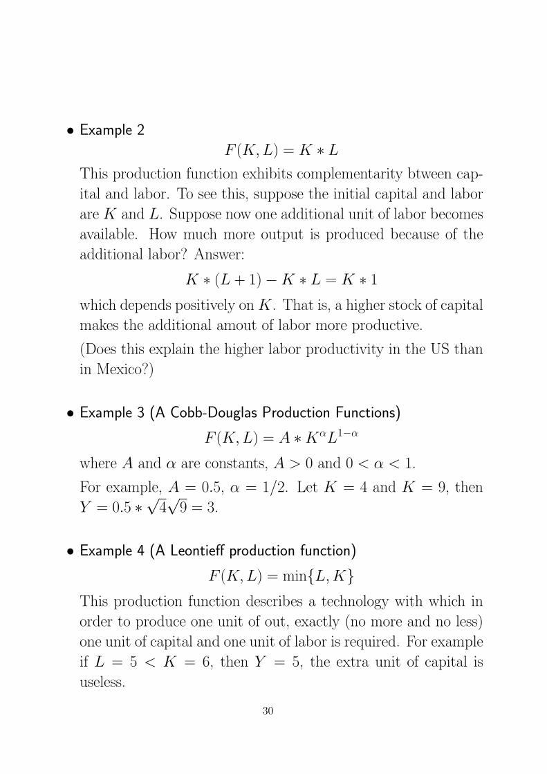
• Example 2
F (K, L) = K ∗ L
This production function exhibits complementarity btween cap-
ital and labor. To see this, suppose the initial capital and labor
are K and L. Suppose now one additional unit of labor becomes
available. How much more output is produced because of the
additional labor? Answer:
K ∗ (L + 1) −K ∗ L = K ∗ 1
which depends positively on K. That is, a higher stock of capital
makes the additional amout of labor more productive.
(Does this explain the higher labor productivity in the US than
in Mexico?)
• Example 3 (A Cobb-Douglas Production Functions)
F (K, L) = A ∗KαL1−α
where A and α are constants, A > 0 and 0 < α < 1.
For example, A = 0.5, α = 1/2. Let K = 4 and K = 9, then
Y = 0.5 ∗√
4√
9 = 3.
• Example 4 (A Leontieff production function)
F (K, L) = min{L, K}This production function describes a technology with which in
order to produce one unit of out, exactly (no more and no less)
one unit of capital and one unit of labor is required. For example
if L = 5 < K = 6, then Y = 5, the extra unit of capital is
useless.
30
• The production function reflects the current technology for turn-
ing capital and labor into output. If someone invents a better
way to produce a good, the result is more output from the same
amounts of capital and labor. Thus, technological change alters
the production function.
• Suppose today’s production function is Y = F (K, L), suppose
tomorrow’s new technology is such that for any given amounts
of capital and labour, output is doubled. Then tomorrow’s pro-
duction function is
Y = 2 ∗ F (K, L)
• Suppose today’s production function is Y = K +L. suppose to-
morrow’s new technology makes tomorrow’s capital twice as pro-
ductive as today’s capital. Then tomorrow’s production function
is
Y = 2 ∗K + L
31
22 Constant Returns to Scale
A production function has constant returns to scale if an increase
of an equal percentage in all factors of production causes an
increase in output of the same percentage. If the production
function has constant returns to scale, then we get 10 percent
more output when we increase both capital and labor by 10
percent.
• Mathematically, a production function has constant returns to
scale if
zF (k, L) = F (zK, zL)
for any positive number z. This equation says that if we multiply
both the amount of capital and the amount of labor by some
number z, output is also multiplied by z.
• Example 1
F (K, L) = K + L
• Example 3
F (K, L) = AKαL1−α
• Example 4
F (K, L) = min{K, L}
32

23 The marginal product of Labor
• The Marginal Product of Labor (MPL) is the extra amount of
output that the economy gets from one extra unit of labor, hold-
ing the amount of capital fixed.
MPL(K, L) = F (K, L + 1) − F (K, L)
That is, MPL is the difference between the amount of output
produced using K units of capital and (L+1) units of labor and
the amount of output produced using K units of capital and L
units of labor.
Important to note: MPL depends on (K, L), the levels of capital
and labor at which MPL is computed.
• Let F (K, L) = K + L. Then
MPL(K, L) = F (K, L+1)−F (K, L) = (K+L+1)−(K+L) = 1
Thus MPL is constant at one for all combinations of K and L.
• Let F (K, L) = KL. Then
MPL(K, L) = K(L + 1) −KL = K.
In this example, MPL depends on K : it is higher when K is
higher.
33
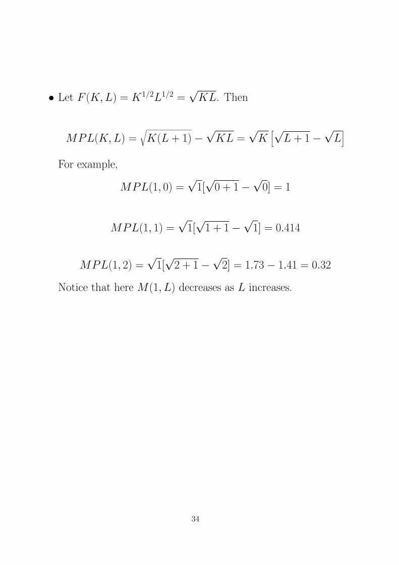
• Let F (K, L) = K1/2L1/2 =√
KL. Then
MPL(K, L) =√K(L + 1) −
√KL =
√K
[√L + 1 −
√L
]
For example,
MPL(1, 0) =√
1[√
0 + 1 −√
0] = 1
MPL(1, 1) =√
1[√
1 + 1 −√
1] = 0.414
MPL(1, 2) =√
1[√
2 + 1 −√
2] = 1.73 − 1.41 = 0.32
Notice that here M(1, L) decreases as L increases.
34
24 The Law of Diminishing Marginal Product
• Many production functions have the property of Diminishing
Marginal Product: Holding the amount of capital fixed, MPL
decreases as L increases.
• Consider the production of bread at a bakery. As a bakery hires
more labor, it produces more bread. As more workers are added
to a fixed amount of capital, however, the MPL falls. Fewer
additional loaves of bread are produced because workers are less
productivewhen the kitchen is more crowded. In other words,
holding the size of the kitchen fixed, each additional worker adds
fewer loaves of bread to the bakery’s output.
• Consider a farmer’s production of potatoes. He has a fixed
amount of land that’s his capital K. Labor input L here is
the number of hours he spends working on his land. Output is
higher as the farmer puts in more effort, but the productivity
(additional output) assoaciated with each additional hour the
farmer puts in declines.
• Professor Wang has a computer that he uses as his capital. Pro-
fessor Wang produces research by spending time with the com-
puter. He is very productive at 9:00 in the morning, he is slower
at 1:00pm, and he feels his brain is useless at 6:30 in the after-
noon.
35
25 The Marginal Product of Capital
The Marginal Product of Capital (MPK) is the extra amount
of output that the economy gets from one extra unit of capital,
holding the amount of labor fixed.
MPL(K, L) = F (K + 1, L) − F (K, L)
That is, MPK is the difference between the amount of output
produced using K + 1 units of capital instead of K units of
capital.
• Let F (K, L) = K + L. Then
MPL(K, L) = F (K+1, L)−F (K, L) = (K+1+L)−(K+L) = 1
Thus MPK is constant at one for all combinations of K and L.
• Let F (K, L) = K ∗ L. Then
MPL(K, L) = (K + 1)L−KL = L.
In this example, MPK depends on L : it is higher when L is
higher.
36
26 MPL and the demand for Labor (1)
• Consider a firm which has a fixed amount of capital and wants
to determine how many workers to hire. Let P denote price and
W be the nominal wage (number of dollars paid to a worker).
• Suppose
P ∗MPL(K, L) > W
Then the firm would want to hire more workers.
• Suppose
P ∗MPL(K, L) < W
Then the firm would want to hire less workers.
• The firm’s equilibrium L is setermined by
P ∗MPL(K, L) = W
or
MPL(K,L) =W
Pwhere W/P is called the real wage.
Figure 3-4.
37
27 MPL and the demand for labor (2)
• We know that given K, the firm’s optimal amount of labor, L∗,
is determined by the following equation
MPL(K,L) =W
P
• Suppose it is now given that
MPL(K, L) = K − L
where K = 10 is fixed. Suppose also W = 10, P = 2. Then L∗
satisfies
10 − L∗ =10
2or
L∗ = 5
• Suppose now the firm has just made some new capital investment
and capital stock has increasesd from 10 to 15. Then the new
L∗ satisfies
15 − L∗ =10
2and L∗ = 10.
• Suppose now the economy is heading into a recession and the
firm has decided to cut capital stock from 15 to 5. Then the new
38
L∗ satisfies
5 − L∗ =10
2and L∗ = 0. That is, the firm is shut down.
28 MPL and the demand for labor (3)
Suppose a firm (or an industry sector) has the following production
function:
Y = F (K, L) = αKL− L2
Then
MPL(K, L) = [αK(L + 1) − (L + 1)2] − [αKL− L2]
= αK − 2L− 1
And so the firm’s optimal choice of its work force, L∗, is determined
by:
MPL(K, L∗) =W
Por
αK − 2L∗ − 1 =W
P
L∗ =1
2
αK − 1 − W
P
Case (1). Suppose the rest of the economy receives a positive demand
shock which makes them want to expand their work force, which in
turn bids up the market wage W . How does this affect this firm’s
L∗?
39
Case (2) The government (worker union) sets a new minimum wage
which is lower than the current market wage. How does this affect
L∗?
Case (3) Suppose the .com industry is collapsing. A large number of
unemployed workers are trying to find jobs in other industries. Our
does this affect this firm’s L∗?
Case (4) Suppose, due to globalization, a higher demand for the firm’s
product drives up P . How does this affect L∗?
Case (5) Suppose the firm succeeded in a major technological inno-
vation that pushes up α. How does this affect L∗ and Y ?
Case (6) Suppose the federal reserve bank increases the interest rate
to make capital more expensive, and the firm decides to reduce its
capital stock. What happens to L∗?
Case (7) Suppose there is a fixed number of workers L̄ in a sector.
This industry has many firms (all have the same production func-
tion). Suppose now α increases to α′. Then every firm will want to
hire more workers at the current wage W . Competition thus bids up
the wage from W to W ′. In the end, no firm will hire more workers,
but W ′ will satisfy
α′K − 2L− 1 = W ′/P.
40
29 Some production functions for you to play with
Consider the following production functions.
F (K, L) = K + 2L
F (K,L) = KL2
F (K, L) = L log(1 + K)L2
(i) Do these production functions show constant returns to scale?
(ii) Do these production functions show diminishing marginal prod-
uct of labor?
30 Equilibrium Employment
Suppose the economy’s production function is Y = F (K, L). Sup-
pose the economy’s capital stock is fixed at K = K, and the econ-
omy’s aggregate labor supply is determined by
Ls = 100 + W
where W denotes market wage. Let M(K, L) denote the marginal
product of labor at K, L.
Then the labor market is in equilibrium if
Ld = Ls(= 100 + W ) (4)
where Ld denotes the aggregate demand for labor and Ld must satisfy
MPL(K, Ld) =W
P. (5)
41
Example 1. Suppose MPL(K, L) = αK − L, where α is constant.
Then equilibrium in the labor market implies:
αK − (100 + W ) =W
P
This equation allows us to solve for the equilibrium wage W ∗, and
then the equilibrium employment is just 100 + W ∗.
42
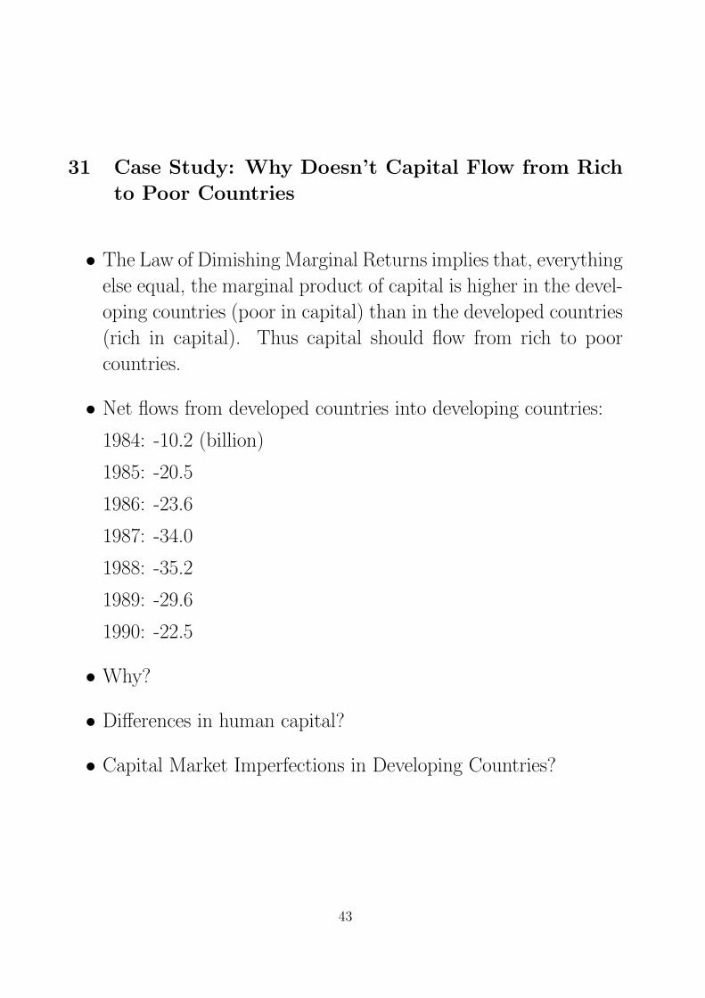
31 Case Study: Why Doesn’t Capital Flow from Rich
to Poor Countries
• The Law of Dimishing Marginal Returns implies that, everything
else equal, the marginal product of capital is higher in the devel-
oping countries (poor in capital) than in the developed countries
(rich in capital). Thus capital should flow from rich to poor
countries.
• Net flows from developed countries into developing countries:
1984: -10.2 (billion)
1985: -20.5
1986: -23.6
1987: -34.0
1988: -35.2
1989: -29.6
1990: -22.5
• Why?
• Differences in human capital?
• Capital Market Imperfections in Developing Countries?
43
Chapter 4The Demand Side of the Economy
• We assume a closed economy - a country that does not trade
with other countries. Thus, net exports are always zero.
• A closed economy has three uses for the goods and services it
produces:
Y = C + I + G
Households consume some of the eocnomy’s output (consump-
tion is the largest soure of demand); firms and households use
some of the output for investment; and the government buys
some of the output for public purposes.
44
32 Consumption: C
• The income that households receive equals the output of the
economy Y. The government then taxes households an amount
T. We define income after the payment of all taxes, Y − T, as
disposable income, denoted
Y d = Y − T
• The level of consumption depends directly on the level of dis-
posable income. The higher is disposable income, the greater is
consumption. Thus,
C = C(Y d)
The relationship between consumption and disposable income is
called the consumption function.
• An example of a consumption function is
C = a + bY d
where a and b are constants.
• The marginal propensity to consume (MPC) is the amount by
which consumption changes when disposable income increases
by one dollar:
MPC(Y d) = C(Y d + 1) − C(Yd)
45
• Usually, the MPC is between zero and one: an extra dollar of
income increases consumption, by less than one dollar. Thus, if
households obtain an extra dollar of income, they save a portion
of it.
• For example, if the MPC is 0.7, then households spend 70 centers
of each additional dollar of disposable income on consumer goods
and services and save 30 cents.
• Suppose
C(Y d) = a + bY d
Then
MPC(Y d) = a + b(Y d + 1) − [a + bY d] = b
• Suppose C(Y d) =√
Y d, then MPC depends on Y d.
46
33 What determines consumption/savings: cases
(1) I am young and poor, but I expect to get wealthier in thefu-
ture. Should I save more (that is consume less) today?
(2) I am young and productive. My wages are high. But I expect
to have my wages fall when I get older. What should do?
(3) In the 1990s, the americans were more optimistic about their
future economic life than ever. Did they save less or more?
(4) The economy is in a recession. But people are starting to
expect things to get better in the near future. Do they save less
or more? What if the consumers are more pessimistic and they
expect the current slump to last for several yearsb (like what
happened in Japan during the 1990s)?
(5) I am employed and healthy. But I may get laid off and
become sick in the future? What should I do?
(6) Your parents had fewer ways to borrow when they needed
liquidity to cover business losses or sickness. I have access to a
financial market where I can lend and borrow, I also have access
to sophisticated insurance policies (private or government spon-
sored) that cover me with benefits and compensation if things
go wrong. Do I save more than my parents?
(7) The Canadians have more extensive social programs (UI,
Medical insurance) than the Americans. Do the Americans save
47

more?
(8) Do married people save more or less?
(9) Interest rare is going up? What should I do?
48
Case Study: Americans are drowning in debt
The American Legacy: Too Much Debt. By the end of 2000,
together consumers owe 7.3 trillion dollars. In 1985, total debt
was below 2 trillion. It doubled over the last ten years.
Americans are also spending more and save less. Total consumer
expenditure went from below 5 trillion in 1995 to above 7 trillion
in 2000. Personal savings rate dropped from 8 percent before
1992 to almost negative in 2000.
Why? Credit cards to be blamed? The new economy phe-
nomenon? A change in Attitude?
Case Study: The Consumption Function: a comparison between
the U.S. and Japan
(handouts)
Why do the Japanese save so much?
Readings: Mankiw: Chapters 3, 17.
49
34 Investment: I
• The main determinant of investment is the interest rate.
• Interest rate measures the cost of the funds used to finance in-
vestment. For an investment project to be profitable, its return
must exceed its cost. If the interest rate rises, fewer investment
projects are profitable, and the quantity of investment goods
demanded falls.
• We suppose there is a single interest rate in the economy. This
is a reasonable assumption because, although there are many
different interest rates in the economy, they tend to move fairly
closely together.
• The nominal interest rate is the interest rate as usually reported:
it is the rate of interest that investors pay to borrow money. The
real interest rate is the nominal interest rate corrected for the
effects of inflation. If the nominal interest rate is 8 percent and
the inflation rate is 3 percent, then the real interest rate is 5
percent.
• The Investment Function relates investment I to the real interest
rate r:
I = I(r).
50
• The investment function is usually downward slopping: When
interest rate rises, financing is more costly, fewer projects are
profitable, demand for investment falls.
Figures 3-6.
51
35 Government Purchases: G
• The third component of aggregate demand is government pur-
chases of goods and services. (Government also makes transfer
payments to individuals and households are not included in G.
Transfer payment contribute indirectly to the aggregate demand
through their effects on consumption.)
• Remember T denotes total taxes. If G > T , then the govern-
ment is running a deficit equal to G − T . If G < T , then the
government has a surplus equal to T − G. If G = T , then the
government has a balanced budget.
52
36 Equilibrium
• The economy’s aggregate supply is determined by:
Y = F (K, L)
• The economy’s aggreagate demand is determined by:
Y D = C(Y − T ) + I(r) + G
• Suppose we treat the following variables as the model’s exoge-
nous variables:
K, L; G, T
That is, we take K, L, G, T as given and not to be determined
by the model. Note once K and L are given, then Y is also
given, which in turn implies C(Y − T ) is also given.
• The model’s only endogenous variable is hence r, the real interest
rate, or the price for the use of capital. r will be determined by
the market.
• The market for goods and services now work to bring aggregate
demand and aggregate supply into balance:
Y = C + I(r) + G
53
• This equation, which is called the equilibrium condition, deter-
mines the equilibrium interest rate r∗. In other words, at the
equilibrium interest rate, the aggregate demand equals aggre-
gate supply.
• As mentioned earlier, the interest rate r is the cost of borrowing
and the retrun to lending (return on investment) in the financial
market.
• Here, if Y > C + I(r) + G, then investment is too low, and
aggregate demand falls short of the aggregate supply, interest
rate will fall as suppliers bid down the price of capital.
• If Y < C + I + G, then investment is too high, and aggregate
demand exceeds the aggregate supply, interest rate will rise as
firms bid up the price of capital.
• Example 1 Suppose Y = 100, G = 10, T = 10. C(Y − T ) =
20 + 0.5(Y − T ), I(r) = 30 − 50r.
Compute the equilibrium r and I .
Aggregate supply equal to aggregate demand implies
100 = (20 + 0.5 ∗ (100 − 10) + 10 + (30 − 50r)
or r = 0.1 and I(r) = 30 − 50 ∗ 0.1 = 25.
54
37 Financial (Credit) Market equilibrium
• Rewrite the equilibrium condition as
Y − C −G = I(r)
where Y −C −G the output that remains after the demands of
consumers and and government are satisfied; it is called national saving
or simply saving (S). Thus the above equation shows saving
equals investment.
• The left hand side of the equation can be thought of as the sup-
ply of loanable funds–households lend their savings to investors
through the financial markets (Direct Lending) or deposit their
saving in a bank that then loans the funds out (Indirect Lending).
• The right hand side of the equation is the demand fopr loanable
funds–investors borrow from the public by selling stocks or bonds
or indirectly by borrowing from banks.
• The price of loanable funds is the interest rate which in the finan-
cial market equilibrium makes demand and supply for loanable
funds equal.
55
38 Public vs Private Saving
• National saving can be split into two parts:
Y − C −G = [Y − T − C] + (T −G)
here Y −T −C is disposable income minus consumption, which
is private saving. T−G is government revenue minus government
spending, which is public saving
• Figure 3-7.
56
39 Policy Analysis: An Increase in G
• An increase in G implies a drecrease in the supply of the loanable
funds. This must be met by a decrease in I(r), the demand for
loanable funds. This effect of an incrtease in G is called the
crowding out effect.
• To induce I(r) to fall, interest rate must increase.
• Example 1 Suppose Y = 100, G = 10, T = 10. C(Y − T ) =
20 + 0.5(Y − T ), I(r) = 30 − 50r. Suppose there is now an
increase in G from 10 to 11.
(b) Compute the new equilibrium I and r.
• Wars and interest in UK, 173−−1920. Figure 3-9.
40 A Decrease in Taxes
• Suppose there is a reduction in taxes of ∆T . Then Y d = Y −T
will increase by ∆T . C(Y d) will increase by MPC ×∆T . This
reduces the supply of loanable funds, So I must decrease and r
must increase. Once again we have a crowing out effect.
• Example 1 Suppose Y = 100, G = 10, T = 10. C(Y − T ) =
20 + 0.5(Y − T ), I(r) = 30 − 50r. Suppose there is now a tax
cut of ∆T = 1.
57
(c) Compute the new equilibrium I and r.
(d) Suppose C(Y − T ) = 20 − M(Y − T ), where M is the
constant MPC. Show that when M increases, more investment
is crowed out due to a fixed amount of tax cut ∆T = 1.
41 Fiscal Policy in the 1980s
• In 1980 Ronald Reagan was elected president. He increased gov-
ernment (military) spending and reduced taxes. The federal
budget deficit skyrocketed in the 1980s. The real interest rate
rose from 0.4 percent in the 1970s to 5.7 percent in the 1980s.
Gross national saving as a percent of GDP fell from 16.7 in the
1970s to 14.1 in the 1980s.
Case Study: Cut Capital Income Taxes to Stop Re-
cession?
• What’s Capital Income Tax?
• Why should Capital Incomes be Taxed? Why should capital
incomes be taxed twice?
• The impact of tax cuts on the budget deficit?—-the “Laffer
Curve”
42 Changes in Investment Demand
• So far we are holding the investment function as given. What
happens if there is a change in the investment function I(r).
58
• For example, what happens if the investment function in Ex-
ample 1 changes from I(r) = 30 − 50r to I(r) = 40 − 50r?
(classwork)
• Figure 3-10
• Example 2 Suppose Y = 100, G = 10, T = 10. C(Y − T, r) =
20 + 0.5(Y − T ) − 10r, I(r) = 30 − 50r.
(a) Compute the equilibrium r and I .
(b) Suppose I(r) = 35 − 50r. Compute the new equilibrium
r and I . Show that with the consumption function downward-
sloping, an increase in investment demand would raise both the
equilibrium interest rate and the equilibrium quanty of invest-
ment.
Case Study: Why do stocks fall when interest rate
rises?
59
43 Equilibrium in the more general setting
• Suppose Y = 100 is fixed. Suppose the consumption function
is C(Y − T ) = 20 + M(Y − T ), where M is a constant that
is between 0 and 1. Suppose the investment function is I(r) =
30 − 50r. Suppose we leave G and T as unspecified constants.
• Remember the equilibrim condition for the economy is
Y − C(Y − T ) −G = I(r)
Subsitute Y = 100 and C = 20+M(Y −T ) and I(r) = 30−50r
into the equilibrium condition to get
100 − [20 + M(100 − T )] −G = 30 − 50r
solve this equation for the equilibrium interest rate
r∗ =50 −M(100 − T ) −G
−50or
r∗ =−50 + M(100 − T ) + G
50
• We can make several predictions based on the above equation.
(1) When G rises, r∗ rises and so I(r∗) falls. This is what we
called the “crowding-out effect”.
(2) When T increases, r∗ decreases and I(r∗) increases. What
happens here is, as T goes up, disposable income Y − T falls,
so consumption falls, and saving goes up, and this induces the
60
supply of loanable funds to go up. What happens next is com-
petition among banks (who all want to find borrowers for their
loanable funds) will bid down the price for the use of funds or
the interest rate.
(3) When M increases, r∗ increases.
• Note given the form of the consumption function, M is equal to
the marginal propensity to consume (MPC). Can you show this?
• Suppose we have two countries. Country 1 (Japan) has a lower
M than country 2 (US). According to our model, Which country
has a lower interest rate?
61
Chapter 5The IS-LM Analysis
44 The Equilibrium GDP (Mankiw Chaper 10-1)
• Let Y denote the economy’s potential GDP. Y is the maximum
amount of goods and services that the economy can produce if
all the economy’s available resources are fully utilitized.
• As before, let Y ∗ be the economy’s equilibrium GDP. Assume
Y ∗ < Y .
That is, the economy is operating at a level that is strictly below
its potential. Imagine the economy is in a recession where many
workers are unemployed and factories are closed.
• Question: That can be done to raise the equilibrium GDP?
• Remember the equilibrium condition for the economy is:
Y = C(Y − T ) + I(r) + G
Note that so far we have always treated Y (together with G and
T ) as the model’s exogenous variable. This time we want to use
the model to determine Y , that is, we now want to assume Y is
the model’s endogenous varable.
62
• To make our life easy, as a first step let’s assume interest r is fixed
(by the Federal Reserve Bank which, we assume, has full control
over the financial market) That is treat r, G and T as the model’s
exogenous varables. Then the equation Y = C(Y −T )+I(r)+G
can be used to determine the only unknown variable: Y .
• One interpretation (Keynes’ interpretation) of the equation Y =
C(Y − T ) + I + G is that the right hand side of the equation
represents the aggregate PLANNED EXPENDITURE and left
hand side the ACTUAL EXPENDITURE.
• Actual expenditure is the amount households, firms, and the
government actually spend on goods and services, and as we
know, it equals the economy’s GDP. Planned expenditure is the
amount households, firms, and the government would like to
spend on goods and services.
• Why should actual expenditure equal planned expenditure in
equilibrium? This is what the KEYNESIAN CROSS explains.
(Figure 10-4).
• Let E denote planned expenditure. Suppose Y > E. That is,
suppose firms are producing more than the private sector and the
government plan to purchase. Firms are forced to accumulate
inventories. When this happens, firms will reduce production
and that reduces Y .
63
• Suppose Y < E. That is, suppose firms are producing less than
the private sector and the government want to purchase. Firms
will run down their inventories. When this happens, firms will
increase production and that increases Y .
• The Keynesian cross shows how Y determined for fixed I , G and
T . Suppose any of these variables change, Y will change.
• Example 1
Suppose G = 10, T = 10. C(Y − T ) = 20 + 0.5(Y − T ),
I(r) = 30 − 50r and r = 0.1. Compute the equilibrium Y .
Substitute G = 10, T = 10. C(Y − T ) = 20 + 0.5(Y − T ),
I(r) = 30−50r, r = 0.1 into the equilibrium condition to obtain
Y = 20 + 0.5(Y − 10) + 30 − 50 ∗ 0.1 + 10
so
0.5Y = 20 − 5 + 30 − 5 + 10 = 50
and Y ∗ = 100.
64
• Consider now the following more general case. Suppose C(Y −T ) = M(Y − T ), where M is the constant MPC. 0 < M <
1. Suppose the investment function I(r) and G and T are left
unspecified.
• Substitute the above information into the equilibrium condition
Y = C(Y − T ) + I(r) + G to obtain
Y = M(Y − T ) + I(r) + G
which implies
Y = MY −MT + I(r) + G
or
(1 −M)Y = −MT + I(r) + G
or
Y ∗ =−MT + I(r) + G
1 −M
• The above equation makes the following predictions:
(1) An increase in G implies an increase in Y ∗.
(2) An increase in T implies a decrease in Y ∗.
(3) An increase in r implies a decrease in Y ∗.
• What happens if the goverment reduces G?
What happens if the goverment reduces T ?
What happens if the Fed reduces r?
65
• Example 2 Suppose G = 10, T = 10. C(Y −T ) = 20 + 0.5(Y −T ), I(r) = 30 − 50r and r = 0.1.
(1) Suppose now the Fed decides to cut interest rate by one per-
cent. Will GDP increase or decrease? By how many percentage
points? (hints) With r = 0.1, Y ∗ = 100. With r = 0.09,
Y ∗ = 101. So GDP goes up by one percent.
(2) Suppose the Fed wants to pursue an interest rate policy
that implements the following (full-employment) policy objec-
tive: Y ∗ = Y and Y = 102. How should the Fed set its interest
rate target.
66
45 Government-Purchases Multiplier (Mankiw 10-
1)
• We now know that an increase in goverment purchases (G) can
cause the equilibrium Y ∗ to increase. We now ask a more specific
question. Suppose we increase G by one unit. Y ∗ will increase
by how many units?
• To prepare for the analysis. Suppose variable y depends on vari-
able x in the following way: y = 2+3x. Now here if we increase
x by 1 unit, then y will increase by 3 nuits.
• Suppose instead y = 2 + Mx where M is some unknown con-
stant. Then an increase in x by 1 unit will cause y to increase
by M units. More generally, an increase in x by ∆x units will
increase y by M × ∆x units.
• We now go back to our model. Suppose the consumption func-
tion is C(Y − T ) = 25 + M(Y − T ), where again M is the
constant MPC. 0 < M < 1. Suppose the investment function
I(r) and G and T are left unspecified.
• Substitute the above information into the equilibrium condition
Y = C(Y − T ) + I(r) + G
to obtain
Y = 25 + M(Y − T ) + I(r) + G
67
which implies
Y = 25 + MY −MT + I(r) + G
or
(1 −M)Y = 25 −MT + I(r) + G
or
Y ∗ =25 −MT + I(r) + G
1 −Mor
Y ∗ =25 −MT + I(r)
1 −M+
G
1 −M
• The above equation shows that an increase in G by one unit will
cause Y ∗ to increase by 11−M units. We call 1
1−M the government-
purchases multiplier.
• Note that since M < 1, the government-purchases multiplier
is greater than one. For example, suppose M = 0.8, then the
government-purchases multiplier is equal to 5. Thus for example
if the government increases its G by 10 billion, then GDP will
increase by 5 × 10 billion.
implies an increase in Y ∗.
(2) An increase in T implies a decrease in Y ∗.
(3) An increase in r implies a decrease in Y ∗.
• What happens if the goverment reduces G?
What happens if the goverment reduces T ?
68
What happens if the Fed reduces r?
• Example 2 Suppose G = 10, T = 10. C(Y −T ) = 20 + 0.5(Y −T ), I(r) = 30−50r and r = 0.1. Suppose now the Fed decides to
cut interest rate by one percent. Will GDP increase or decrease?
By how many percentage points?
(hints) With r = 0.1, Y ∗ = 100. With r = 0.09, Y ∗ = 101. So
GDP goes up by one percent.
69
46 Case Study: Cutting Taxes to Stimulate the
Economy
In 1961, John F. Kennedy became president of the United States.
FKK brought to Washington a group of bright young economists
to work on his Council of Economic Advisers. These economists
were educated in the school of Keynesian economics.
One of .... (see Mankiw page 266 (a very nice page))
47 The IS curve
If both r and Y are treated as variables, not constants. Then
Y = C(Y − T ) + I(r) + G describes a relationship between r
and Y . This relationship is called the IS curve. There I means
investment S means saving.
48 A Loanable-Funds Interpretation of the IS equa-
tion
The equilibrium condition Y = C(Y − T ) + I(r) + G can be
rewritten as
Y − C(Y − T ) −G = I(r)
70
• Remember in the model of Y = C(Y − T ) + I(r) + G, we have
either assumed Y is fixed and then used the model to determine
the endogenous variable r, or we have assumed r is fixed and
used the model to determine Y as the endogenous variable.
But both Y and r are important macroeconomic variables that
economists want to explain and make predictions about. It is
thus desirable to treat both Y and r as endogenous variables.
To goal here is to build a model that does exactly that.
• Suppose we now treat both Y and r as our model’s endogenous
variables. Then the equation
Y = C(Y − T ) + I(r) + G (6)
is called the IS equation or IS curve.
• The IS equation provides a link between r and Y , but it is not
enough for determining both r and Y . All we need is one more
equation that links r and Y together. We look into the money
market to find that missing equation.
71
49 Money
• What is Money? Economists use the term money to mean specif-
ically the stock of assets that can be readily used as a medium
of exchange to make transactions.
• The measure of the quantity of money usually includes currency
and demand deposits.
Currency is the sum of outstanding paper money and coins. Most
day-to-day transactions use currency as the medium of change.
Demand deposits represent the funds people hold in their check-
ing account. Assets in a checking account are almost as conve-
nient as currency.
• Money, once defined as currency and checking deposits, is the
type of asset that does not earn interest for its holder.
• There are other more broadly defined measures of money which
include for instance saving deposits, time deposits, and Treasury
securities.
72
50 The Demand for Money
• Let M denote the amount of money balances. Let Md denote
the demand for (nominal) money balances. Let M s denote the
supply of (nominal) money balances. Let P denote the price
level.
Note in the model we are developing, both M s and P will be
treated as exogenous variable. In particular, M s will be treated
as a policy instrument for the Federal Reserve Bank for conduct-
ing monetary policy.
• Assume the demand for money is described by
Md = P × L(r, Y )
where r is the interest rate, Y is the GDP or national income,
and the function L is called the money demand function.
• This money demand function states that the demand for money
varies proportionally with the price level. That is, if the level of
price changes by a certain percent, then the demand for money
will change by the same percent.
• The demand for money decreases as r increases. That is, holding
Y constant, the money demand function L(r, Y ) is downward
sloping in r. The idea is that the interest rate is the opportunity
cost of holding money: it is what you forgo by holding some of
your financial assets as money.
73
• On the other hand, an increase in Y causes the demand for
money to also increase. The idea here is that when Y increases,
more buying and selling will take place that requires the use of
money to make payments.
• The money demand equation can also be written as:
Md
P= L(r, Y ) (7)
where Md
P is called the demand for real money balances.
74
51 Money Market Equilibrium
• When the money market is in equilibroum, the demand for
money must be equal to the supply of money:
M s = Md
or,
M s = P × L(r, Y )
or
M s
P= L(r, Y ) (8)
The above equation is called the equilibrium condition for the
money market. It is also called the LM equation or LM curve.
75
• Example1 Let
L(r, Y ) = 100 − r + 0.5Y
Let M = 100 and P = 1. Then the LM equation is
100/1 = 100 − r + 0.5Y
or
r = 0.5Y
This equation says in order for the money market to clear, inter-
est rate must increase as Y increases.
• Suppose again L(r, Y ) = 100 − r + 0.5Y and P = 1. But we
leave M s unspecified. The the IS curve is
M s = 100 − r + 0.5Y
which in turn implies
r = 100 −M s + 0.5Y
This shows that, holding Y fixed, an increase in money supply
reduces the interest rate.
76
52 The IS − LM Analysis
• We now put the IS and LM equations together to ontain a
system of two equations with two unknowns:
IS : Y = C(Y − T ) + I(r) + G
LM :M s
P= L(r, Y )
where T,G,M s and P are exogenous variables.
Example1
Let T = G = 0. Let C(Y − T ) = 0.5(Y − T ). Let I(r) =
100 − 10r. Let P = 1 and L(r, Y ) = Y − 10r. Let M s be left
unspecified.
Then the the IS equation is
Y = 0.5Y + 100 − 10r
or
Y = 200 − 20r
and the LM equation is
M s = Y − 10r
Substitute the IS equation into the LM equation to get
M s = 200 − 20r − 10r = 200 − 30r
77
and so
r∗ = (200 −M s)/30
and
Y ∗ = 300 − 20 ∗ (200 −M s)/30.
Clearly, as M s increases, Y ∗ increases and r∗ decreases.
Suppose initially M s = 100. Suppose there is now a productivity
slowdown which shifts the investment function to
I(r) = 90 − 10r,
which, in turn, drives the economy into a “recession”.
Now as an economist you know several ways through which you
can pull the economy back from the recession and restore the
initial Y ∗.
(1) Suppose you want to pursue an expansionary monetary pol-
icy to offset the effect of the lower investment. By how many
percentage points should increase M s?
(2) What are other policy changes you can pursue to achieve the
same objective?
78
We now take a step further to consider the more general situation
where all of the three policy instruments, T , G, and M s are left
unspecified. This will allow us to consider both the fiscal and
the monetary policies in one comprehensive model.
Let C(Y − T ) = C0 + m(Y − T ). Let I(r) = I0 − 10r. Let
P = 1 and L(r, Y ) = Y − 10r. Let T,G, and M s be left
unspecified. Note here 0 < m < 1 is the consumer’s constant
marginal propensity to consume.
The IS equation is
Y = C0 + I0 + m(Y − T ) − 10r + G
or
(1 −m)Y = C0 + I0 −mT − 10r + G
The LM equation is
M s = Y − 10r
From the LM equation we have Y = M s + 10r. Substitute this
into the IS equation to get
(1 −m)(M s + 10r) = C0 + I0 −mT − 10r + G
or
(1 −m)M s + 10(1 −m)r = C0 + I0 −mT − 10r + G
and so
[10(1 −m) + 10]r = C0 + I0 −mT + G− (1 −m)M s
79
and so
r∗ =C0 + I0 −mT + G− (1 −m)M s
20 − 10m(9)
Substitute the above into the LM equation to obtain
Y ∗ = M s + 10r∗ = M s + 10C0 + I0 −mT + G− (1 −m)M s
20 − 10mor
Y ∗ =M s −mT + G + C0 + I0
2 −m(10)
• Clearly, as M s increases, Y ∗ increases and r∗ decreases. As G
increases, Y ∗ increases and r∗ increases. As T increases, Y ∗
decreases and r∗ decreases.
• The above equation shows that an increase in G by one unit
will cause Y ∗ to increase by 12−m units. Thus here 1
1−m is the
government-purchases multiplier.
• Note that since M < 1, now the government-purchases multi-
plier is less than one.
Example 3(classwork) Suppose G = 10, T = 10. C(Y − T ) =
0.5(Y − T ), I(r) = 100 − 10r. Suppose M s = 100, P = 1 and
L(r, Y ) = Y −10r. Suppose now the Fed decides to cut interest
rate by one percentage point, should the Fed increase money
supply by how many units? Will GDP increase or decrease? By
how many percentage points?
80
53 Fiscal and Monetary Policy Design
The central bank sees inflation rising in the future. It then wants
to tighten up monetary policy to fight that. But a tight monetary
policy is likely to raise interest rate and that in turn may have a
negative effect on the stock market.
Can you design a monetary and fiscal policy combination to slow
down the economy while not raising the interest rate?
81
54 Creating a Recession
Suppose you given a toy economy to play with. Suppose this
toy economy is described by the equations you are familar with.
How can you create a recession in this economy?
82
55 The Great Depression
See Table 11-2 for the statistics regarding the great depression.
What caused the great depression?
Theory 1 A downward shift in the consumption function caused
the contractionary shift in the IS curve. The stock market crash
of 1929 may have been partly responsible for this shift: by reduc-
ing wealth and increasing uncertainty about the future prospects
of the U.S. economy, the crash may have induced consumers to
save more of their income rather than spending it.
Theory 2 The great depression was caused by the large drop in
investment in housing. Some economists believe that the residen-
tial investment boom of the 1920s was excessive and that once
this overbuilding became apparent, the demand for residential
investment declined drastically. Another possible explanation
for the fall in residential investment is the reduction in immigra-
tion in the 1930s: a more slowly growing population demands
less new housing.
Theory 3 Many banks failed in the early 1930s, in part because
of inadequate bank regulation, and these bank failures may have
exacerbated the fall in investment spending. Banks play the
crucial role of getting the funds available for investment to those
households and firms that can best use them. The closing of
many banks in the early 1930s may have prevented some busi-
nesses from getting the funds they needed for capital investment
83
and, therefore, may have led to a further contractionary shift in
the investment function.
Theory 4 In addition, the fiscal policy of the 1930s caused a
contractionary shift in the IS curve. Politicians at that time were
more concerned with balancing the budget than with using fiscal
policy to keep production and employment at their natural rates.
The Revenue Act of 1932 increased various taxes, especially those
falling on lower- and middle-income consumers.
Theory 5 The money supply fell 25 percent from 1929 to 1933,
during which time the unemployment rate rose from 3.2 percent
to 25.2 percent. Friedman and Schwartz argue that contractions
in the money supply have caused most economic downturns and
that the Great Depression is a particularly vivid example.
A problem for this hypothesis is the behavior of interest rates.
If a contractionary shift in the LM curve triggered the Depres-
sion, we should have observed higher interest rates. Yet nominal
interest rates fell continuously from 1929 to 1933.
Theory 6 From 1929 to 1933 the price level fell 25 percent. Many
economists argue that the deflation may have turned what in
1931 was a typical economic downturn into an unprecedented
period of high unemployment and depressed income.
84
56 The Effects of Deflation
Effect 1 For any given supply of money M, a lower price level
implies higher real money balances M/P. An increase in real
money balances causes an expansionary shift in the LM curve,
which leads to higher income.
Effect 2 Another channel through which falling prices expand in-
come is called the Pigou effect. As prices fall and real money
balances rise, consumers should feel wealthier and spend more.
This increase in consumer spending should cause an expansion-
ary shift in the IS curve, also leading to higher income.
Effect 3: The debt-deflation theory An unexpected deflation makes
debtors poorer and creditors richer. Debtors thus spend less and
creditors spend more. If these two groups have equal spending
propensities, there is no aggregate impact. But it seems reason-
able to assume that debtors have higher propensities to spend
than creditors perhaps that is why the debtors are in debt in
the first place. In this case, debtors reduce their spending by
more than creditors raise theirs. The net effect is a reduction in
spending.
Effect 4 When firms come to expect deflation, they become re-
luctant to borrow to buy investment goods because they believe
they will have to repay these loans later in more valuable dollars.
The fall in investment depresses planned expenditure, which in
turn depresses income.
85
57 The Japanese Slump
During the 1990s, after many years of rapid growth and enviable
prosperity, the Japanese economy experienced a prolonged down-
turn. Real GDP grew at an average rate of only 1.3 percent over
the decade, compared with 4.3 percent over the previous twenty
years. The unemployment rate, which had historically been very
low in Japan, rose from 2.1 percent in 1990 to 4.7 percent in 1999.
In August 2001, unemployment hit 5.0 percent, the highest rate
since 1953.
Although the Japanese slump of the 1990s is not even close in
magnitude to the Great Depression of the 1930s, the episodes
are similar in several ways.
First, both episodes are traced in part to a large decline in stock
prices. In Japan, stock prices at the end of the 1990s were less
than half the peak level they had reached about a decade earlier.
Like the stock market, Japanese land prices had also skyrockeded
in the 1980s before crashing in the 1990s.
Second, during both episodes, banks ran into trouble and ex-
acerbated the slump in economic activity. Japanese banks in
the 190s had made many loans that were backed by stock or
land. When the value of this collateral fell, borrowers started
defaulting on their loans. These defaults on the old loans re-
duced the banks ability to make new loans. The resulting credit
crunch made it harder for firms to finance investment projects
86
and, thus, depressed investment spending.
Third, both episodes saw a fall in economic activity coincide
with very low interest rates. This fact suggests that the cause of
the slump was primarily a contractionary shift in the IS curve,
because such a shift reduces both income and the interest rate.
The obvious suspects to explain the IS shift are the crashes in
stock and land prices and the problems in the banking system.
Finally, the policy debate in Japan mirrored the debate over
the Great Depression. Some economists recommended that the
Japanese government pass large tax cuts to encourage more con-
sumer spending. Although this advice was followed to some ex-
tent, Japanese policymakers were reluctant to enact very large
tax cuts because, like the U.S. policymakers in the 1930s, they
wanted to avoid budget deficits. In Japan, this is in part because
the government was facing a large unfounded pension liability
and a rapidly aging population.
Other economists recommended that the Bank of Japan expand
the money supply more rapidly. Even if nominal interest rates
could not go much lower, they perhaps more rapid money growth
could raise expected inflation, lower real interest rates, and stim-
ulate investment spending. Thus, although economists differed
about whether fiscal or monetary policy was more likely to be
effective, there was wide agreement that the solution to Japans
slump, like the solution to the Great Depression, rested in more
aggressive expansion of aggregate demand.
87
58 The Liquidity Trap
In Japan in the 1990s and the United States in the 1930s, interest
rates reached very low levels. As Table 11-2 shows, U.S. interest
rates were well under 1 percent throughout the second half of
the 1930s. The same was true in Japan during the second half
of the 1990s. In 1999, Japanese short-term interest rates fell to
about one-tenth of 1 percent.
Some economists describe this situation as a liquidity trap. Ac-
cording to the IS-LM model, expansionary monetary policy works
by reducing interest rates and stimulating investment spending.
But if interest rates have already fallen almost to zero, then per-
haps monetary policy is no longer effective.
Other economists are skeptical about this argument. One re-
sponse is that expansionary monetary policy might raise infla-
tion expectations. Even if nominal interest rates cannot fall any
further, higher expected inflation can lower real interest rates by
making them negative, which would stimulate investment spend-
ing. A second response is that monetary expansion would cause
they currency to lose value in the market for foreign-currency ex-
change. This depreciation would make the nations goods cheaper
abroad, stimulating export demand.
88
Chapter 6The Open Economy
59 The open Economy
So far we have studied a closed economy. Let’s now open the
economy up for international trade.
Remember the GDP can be divided into the following compo-
nents:
Y = Cd + Id + Gd + EX
where Cd is (domestic) consumption expenditure on domestic
goods and services, Id is (domestic) investment expenditure on
domestic goods and services, Gd is (domestic) government pur-
chases of domestic goods and services. EX is (total) exports of
domestic goods and services.
Cd+Id+Gd is domestic spending on domestic goods and services.
EX is foreign spending on domestic goods and services.
Cf is (domestic) consumption expenditure on foreign goods and
services. If is (domestic) investment expenditure on foreign
goods and services, Gf is (domestic) government purchases of
foreign goods and services.
IM = Cf + If + Gf
89
is total imports, or total domestic spending on foreign goods and
services.
C = Cd + Cf
I = Id + If
G = Gd + Gf
Substitute the above into Y = Cd + Id + Gd + EX to obtain
Y = C + I + G + EX − (Cf + If + Gf)
or
Y = C + I + G + EX − IM
or
Y = C + I + G + NX (11)
where
NX = EX − IM
is net exports, or trade balance.
The equation Y = C + I + G + NX can be rewritten as
NX = Y − (C + I + G) (12)
That is, net exports is equal to output minus domestic spending.
If the economy produces more than it spends, then net exports is
positive (Trade surplus). Otherwise it’s negative (trade deficit).
When NX = 0, the economy is said to have balanced trade.
90
60 International Capital Flows and the Trade Bal-
ance
Let S = Y − C − G denote national saving (it is equal to the
sum of publc saving T −G and private saving Y −T −G). Then
the equation Y = C + I + G + NX can be rewritten as
S − I = NX
That is, the economy’s net exports (trade balance) must always
be equal to the difference between its saving and its investment.
S − I is called net capital outflow.
That is, if the domestic economy saves more than it invests, then
the surplus flows to the foreign countries.
If our investment exceeds saving, then the net capital flow is
negative. That is, we must borrow from foreign countries to
finance our investment.
In other words,
Net Capital Outflow = Trade balance
One way to think about the above equation is this: When S >
I , we are saving more than we invest. What’s saved but not
invested is used to make loans to foreigners. These loans enables
the foreigners to buy more goods and services from us than we
91
buy from them. Eventually, the loans will become goods and
services exported to foreign countries.
On the other hand, if Our investment exceeds our saving, the
extra investment must be financed by borropwing from abroad.
These foreign loans enables us import more goods and services
than we export. That is, we are running a trade deficit.
International flow of capital may take many forms. In other
words, there are many ways in which international lending and
borrowing can take place. When the US runs a trade deficit with
Japan, the capital flow from Japan to the US could take the form
of a financial loan make to a US company by a Japanese bank, or
the Japanese buying the debt issued by American corporations,
or the Japanese buy other types of US assets (equity, treasury
bills, houses).
92
61 A Small Open Economy
Consider first a small open economy with perfect capital mobility.
Small means the economy is a small and negligible part of the
world financial market and it has no way to affect the determi-
nation of the world interest rate.
By perfect market mobility we mean that residents of the
country have full access to world financial markets. In particular,
the government does not interfere with international lending and
borrowing.
Let r∗ denote the world interest rate (market rate in the world
financial markets).
Because of perfect market mobility, residents of the small open
economy need never brrow at any interest rate above r∗, they
need never lend at a rate that is lower than r∗ either. So, in our
small open economy,
r = r∗.
93
Now as we did for the closed economy, let’s first assume the
economy’s output Y is fixed. Assume C = C(Y − T ) and
I = I(r). Because r = r∗, so I = I(r∗).
So the economy’s net exports must be equal to
NX = [Y − C(Y − T ) −G] − I(r∗)
The above equation can be used to consider how policies influ-
ence the trade balance.
For example, an increase in G reduces trade surplus and increases
trade deficit.
94
62 Exchange Rates
The nominal exchange rate is the relative price of the currency
of two countries.
Suppose the exchange rate between the US dollar and the Japanese
yen is 120 yen per dollar. Then you can use 1 dollar to buy 120
yen, or you can pay 120 yen to buy 1 dollar.
When people refer to the exchange rate, they usually mean the
nominal exchange rate.
We use e to denote the nominal exchange rate.
1 dollar = e yen
1 domest currency = e foreign currency
The real exchange rate is the relative price of the goods of the
two countries. Suppose there is only one good, cars, that the
two economy produce and the American cars and Japanese cars
of of the same quality. Then the real exchange rate is the price
of one US (domestic) car in units of Japanese (foreign) cars. In
other words, in order to buy one US car, how many US cars I
must give up.
That is, instead of asking one unit of domestic curreny is equal
to how many units of foreign currency, I now ask one domestic
car is equal to how many foreign cars.
95
We use ε to denote the real exchange rate.
For simplicity, let’s suppose the two countries produce cars only,
and the american cars and the Japanese cars are of the same
quality.
Let P denote the price of a car in the US (the domestic country),
P ∗ the price of a car in Japan.
The question is: one US car is equal to how many Japanese cars?
ε = 1 × P × e/P ∗ = e× (P/P ∗)
Tha is, I sell 1 US car to get 1× P US dollars, I then exchange
them for 1 × P × e Japanese yen, and I then use these yen to
buy 1 × P × e/P ∗ Japanese cars.
The real exchange rate is also called the terms of trade.
96
63 The Mundell-Fleming MOdel
Consider again a small open ecomnomy with perfect capital mo-
bility. We have:
r = r∗
where remember r is the interest rate in the domestic country,
r∗ is the world interest rate.
Assume the goods market is described by the following IS equa-
tion:
Y = C(Y − T ) + I(r∗) + G + NX(e)
The above equation assume that the demand for net exports
depends on the exchange rate. Naturally, NX decreases as e
increases.
The IS curve slopes downward. Figure 12-1(a).
The LM equation now reads
M/P = L(r∗, Y ).
The M-F model is designed to analyze short-term fluctuations,
the price level P is assumed to be exogenously fixed.
We now use this model for policy analysis.
97
64 Floating Exchange Rates
Suppose the government stimulates domestic spending by in-
creasing government purchases or by cutting taxes. This shifts
the IS curve to the right and, as a result, the exchange rate
appreciates, whereas the level of income remains the same.
Suppose the central bank increases the money supply. Because
the price level is assumed to be fixed, this increases the real
money balances, shifting the LM curve to the right. exchange
rate is lower, income higher.
Suppose the government pursues a trade policy to reduce the
demand for imported goods (say by imposing an import qiota
or a tariff). This shifts the NX curve to to right (by reducing
imports), which in turn shifts the IS curve to the right. The ex-
change rate will appreciate but income remains the same. Notice
NX(e) = Y − C(Y − T ) − I(r∗) − G remains the same. So
restricting trade don’t necessarily improves the balance of trade.
98
65 The Fixed Exchange Rate System
99

66 Speculative Attacks and the 1997 Asian Finan-
cial Crisis
100

Chapter 7The New Economy
67 The Concept
• The term New Economy has, more than anything, been associ-
ated with the information technology (IT), computers and the
internet.
• Some believe that IT represents an invention of the method of
inventing, in the sense that it makes researcher more productive
given the fast access to relevant information and faster ways to
handle data; and in the sense of the democratization of knowledge :
computers and the internet makes knowledge available to every-
one who has access to the web.
• This means that we will probably see a wave of new technolo-
gies, new products, new firms, and faster productivity growth
worldwide than we saw during the past century.
101
68 Fictures of the new economy
• The numberof patents The average number of patents issued
annually before 1985 is about 300 per million people, in 1997
this number is approximately 700.
• The stock market
• Merger and takeover waves
• CEO Compensation
• IPOs and new economy companies
102

69 Globalization
103