Macroeconomic Model Spillovers and Their Discontents

Tamim Bayoumi and Francis Vitek

WP/13/4

© 2013 International Monetary Fund WP/13/4

IMF Working Paper

Strategy, Policy, and Review Department

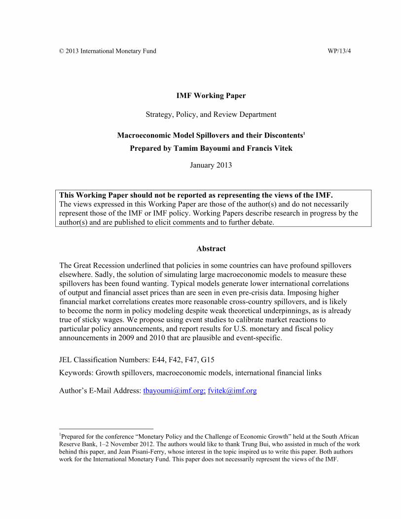
Macroeconomic Model Spillovers and their Discontents1

Prepared by Tamim Bayoumi and Francis Vitek

January 2013

Abstract

The Great Recession underlined that policies in some countries can have profound spillovers elsewhere. Sadly, the solution of simulating large macroeconomic models to measure these spillovers has been found wanting. Typical models generate lower international correlations of output and financial asset prices than are seen in even pre-crisis data. Imposing higher financial market correlations creates more reasonable cross-country spillovers, and is likely to become the norm in policy modeling despite weak theoretical underpinnings, as is already true of sticky wages. We propose using event studies to calibrate market reactions to particular policy announcements, and report results for U.S. monetary and fiscal policy announcements in 2009 and 2010 that are plausible and event-specific.

JEL Classification Numbers: E44, F42, F47, G15

Keywords: Growth spillovers, macroeconomic models, international financial links

Author’s E-Mail Address: tbayoumi@imf.org; fvitek@imf.org

1Prepared for the conference “Monetary Policy and the Challenge of Economic Growth” held at the South African Reserve Bank, 1–2 November 2012. The authors would like to thank Trung Bui, who assisted in much of the work behind this paper, and Jean Pisani-Ferry, whose interest in the topic inspired us to write this paper. Both authors work for the International Monetary Fund. This paper does not necessarily represent the views of the IMF.

This Working Paper should not be reported as representing the views of the IMF. The views expressed in this Working Paper are those of the author(s) and do not necessarily represent those of the IMF or IMF policy. Working Papers describe research in progress by the author(s) and are published to elicit comments and to further debate.

2

Contents Page

I. Introduction ............................................................................................................................3 

II. Large Models: Theory ...........................................................................................................3 

III. Large models: Practice .........................................................................................................6 

IV. A Practical Solution ...........................................................................................................11 

V. Conclusions .........................................................................................................................13  Tables 1. Spillovers from U.S. Monetary Policy: Typical Model .......................................................15 2. Spillovers from U.S. Fiscal Policy: Typical Model .............................................................15 3. Correlations of Quarterly Output Growth, 1980–2012 ........................................................15 4. Spillovers from U.S. Bond and Equity Shocks to Other Countries .....................................16 5. Spillovers from U.S. Monetary Policy: High Financial Links .............................................16 6. Spillovers from U.S. Fiscal Policy: High Financial Links...................................................17 7. Spillovers from U.S. Fiscal Policy: Only High Bond Market Links ...................................17 8. Growth Spillovers from QE1 and QE2 Monetary Easing ...................................................18 9. Growth Spillovers from 2009 and 2010 U.S. Fiscal Expansions ........................................18  Figures 1. U.S. Monetary Policy Spillovers: Typical Model ................................................................19 2. U.S. Fiscal Policy Spillovers: Typical Model ......................................................................19 3. U.S. Monetary Policy Spillovers: High Financial Links .....................................................20 4. U.S. Fiscal Policy Spillovers: High Financial Links ...........................................................20 5. U.S. Fiscal Policy Spillovers: High Bond Market Links .....................................................21 6. Growth Spillovers from QE1 and QE2 Monetary Easing ...................................................21 7. Growth Spillovers from 2009 and 2010 Fiscal Expansions .................................................22  References ................................................................................................................................23 

3

I. INTRODUCTION

The size and composition of spillovers across countries is one of the many issues that

have resurfaced in the wake of the Great Recession. It is now apparent that events in some countries can have profound spillovers elsewhere which are not limited to their immediate neighbors but can ricochet around the globe. This prompts many questions about the advantages of international cooperation and the inadvisability of allowing countries to focus solely on their own domestic stability. Such considerations pertain both to systemic countries and to the aggregate behavior of smaller countries if they are following similar policies.

At first blush, the solution to measuring spillovers across countries would seem to be fairly easy. Why not simply feed relevant shocks into existing large empirically estimated macroeconomic models? After all, these models are designed to capture complex policy dependent interactions across different sectors and countries. In addition, such models have gained increasing respect in the economics profession as they have become more theory-based.

Sadly, this strategy has been found wanting. As currently constructed, most large macroeconomic models have weak spillovers across countries. The reason for this is that the main apparent source of large spillovers is close linkages across financial markets. Although progress is being made, the financial sectors in large macroeconomic models are poorly developed and, at an even more basic level, there are no strong theories as to why financial markets are as closely linked as they appear to be in the data.2 Assuming such links exist creates what look to be sensible results, but at the cost of theoretical rigor. In a sense this is a rerun of the sticky prices debate, which also pitted—and continues to pit—the ability to explain the data against the desire for a sound theoretical substructure.

The rest of this paper explains why standard macroeconomic models fail to deliver the financial market results seen in the data, discusses how this limits measured spillovers, and offers an (imperfect) short-term fix that can be used while the deeper theoretical issues are being sorted out.

II. LARGE MODELS: THEORY

There are three major potential conduits for global spillovers between countries:

trade, commodity prices, and financial markets. Large macroeconomic models typically model trade linkages quite well, at least for final goods trade. The demand elasticities of

2Most of the work is in closed economy settings, see Brunnermeier, Eisenbach, and Sannnikov, 2012.

4

trade with respect to domestic demand (for imports) and foreign demand (for exports) are relatively well known, as is the sensitivity of trade to terms of trade fluctuations. As a result, trade spillovers are typically fairly similar across large models (Bryant, 1988), which tend to abstract from intermediate goods trade, potentially attenuating or distorting spillovers somewhat. While not quite as homogenous, links through commodity prices (which tend to be second order effects outside of commodity producers) show similar patterns.

The least developed area in these multiple country macroeconomic models is financial markets. The underlying financial structure of most models comprises a monetary policy rule that explains the short-term interest rate backed by a Phillips curve that links inflation to the domestic cycle and an expectations hypothesis that translates the expected future path of the short-term interest rate into a long-term interest rate. There may also be an equity price, based on the expected discounted value of future profits. Cross-country holdings of assets are generally modeled very simply—either all assets are priced in a single currency or cross-country asset holdings are held in fixed proportions—given the difficulties in modeling portfolio choice in an already complex model.

Breaking down each of these components in turn, monetary policy is generally assumed to follow a Taylor rule in which the short-term policy interest rate is driven by the deviation of inflation from its desired level and the output gap (the exchange rate can also be included as a target, but does not make much difference to the basic argument). That is:

Short-term interest rate = Taylor rule (Past short-term interest rate; Deviation of inflation from target; Output gap; Monetary policy shock) (1)

Numerous equations of this type have been estimated, and the empirical evidence for them is strong.

Inflation in turn is generally assumed to be a function of past and expected future inflation, the output gap, as well as changes in the terms of trade, which in turn responds to the exchange rate and commodity prices. For example:

Inflation = Phillips curve (Past and expected future inflation; Output gap; Current, past, and expected future terms of trade changes; Supply shock) (2)

Again, this Phillips curve has a long empirical pedigree and is generally accepted as a strong empirical regularity.

Substituting this into the Taylor rule, short-term interest rates are largely driven by current, past and expected future output gaps, as well as the exchange rate and commodity prices. In practice, the impact of commodity prices is generally limited as their weight in the overall consumption basket is often small and they are assumed to approximately follow a

5

random walk. Note also that while changes in commodity prices induce a common component in inflation rates across countries, this impact is dissipated by the exchange rate response which—by definition—creates a divergent effect (if one exchange rate appreciates, another needs to depreciate). In short, unless there is a large commodity price shock the external factors are unlikely to create significant comovements in inflation across countries.

The expectations theory says that the long-term interest rate is the expected average value of the short-term interest rate over the term of the security plus a country-specific liquidity premium that is generally modeled as fixed. That is:

Long-term interest rate = Yield curve (Current and expected future short-term interest rates; Liquidity premium) (3)

There is considerable evidence that expected future domestic monetary policy does impact bond yields, even if the effects are not always of the size that one might expect from first principles.3

It is clear from the third equation that the correlation of short-term and long-term interest rates across countries should be very similar as one is simply an average of the expected future path of the other. If short-term interest rates across countries are highly (lowly) correlated then long-term interest rates will also be highly (lowly) correlated.

As short-term interest rates are driven by the output gap, it follows that financial markets will only be closely linked in response to real shocks if output is correlated across countries through non-financial links. A similar basic story can be told about the correlation of equity prices across countries. Equity prices reflect the expected future discounted earnings of firms and are again driven by the business cycle in each country. Home bias in equity holdings implies that comovements in equity wealth across countries are limited. Hence, equity prices will again only be closely linked if non-financial factors drive an international business cycle.

Furthermore, the correlations with regard to monetary policy shocks can even be perverse. Consider a loosening of monetary policy in any one country that drives down domestic bond yields. As this tends to boost activity both at home and abroad, policy interest rates and hence bond yields will tend to rise elsewhere. Thus standard models predict a negative relationship across bond markets in response to monetary policy shocks.

3Gürkenyak, Sack and Swanson (2005), Bernanke, Reinhart and Sack (2004), and Swiston (2007).

6

III. LARGE MODELS: PRACTICE

In their unadulterated form, large models of the type described above predict low

correlations of output across countries, except between extremely close trading partners (such as Canada and the United States). The reason for this is that the main route though which spillovers can occur is trade, but the comingling of countries’ output via trade is small. While a country can be quite open to trade (often as much as 30 percent of output is imported and exported) this reflects trade across a wide range of partners. Trade with individual countries is rarely particularly large, especially for large countries whose trade patterns tend to be highly diversified.

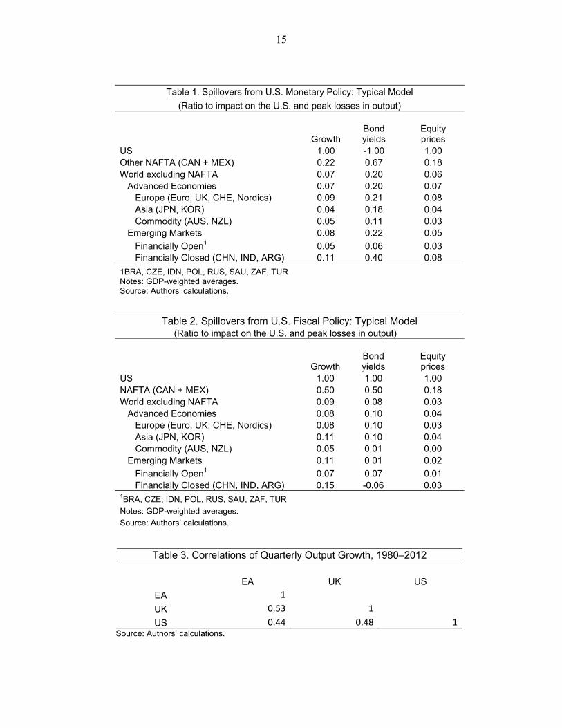
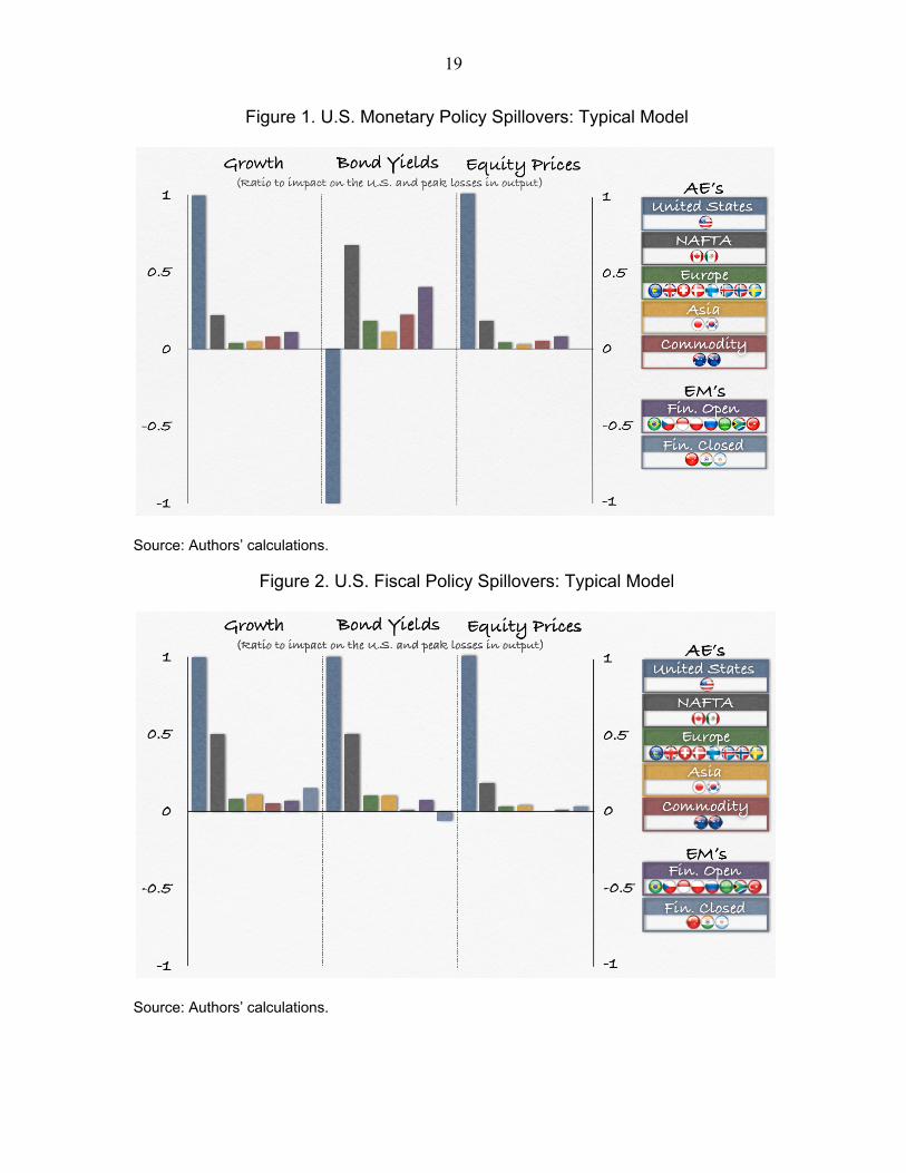
To illustrate these limited spillovers the first column of Table 1 and Figure 1 report the peak impact on output compared to the impact on the United States from a short-term monetary loosening in a fairly typical large macroeconomic model.4 This estimated semi-structural model covers 35 countries, each of which is represented by interconnected real, external, monetary, fiscal, and financial sectors. Within this framework, spillovers are transmitted via trade, commodity price, and financial linkages. There are notable positive output spillovers on the two close NAFTA trading partners (Canada and Mexico) where the peak output gains comprise around one-fifth of those in the United States—slightly more for Canada and less for Mexico.

The macroeconomic model under consideration features direct financial linkages, through both generalized uncovered interest parity relationships connecting money markets, and an international financial accelerator mechanism (and hence takes account of financial frictions) linked to the real value of an internationally diversified equity portfolio. Bond yields are linked to money market interest rates via generalized expectations theory relationships, while equity prices are linked to these interest rates via generalized dividend discount relationships. Nevertheless, outside of NAFTA, spillover coefficients are small—they average 7 cents per dollar. The only other group of countries with a spillover coefficient of over 10 cents is for emerging markets with closed capital accounts (comprising China, India, and Argentina), reflecting the close trading links between China and the United States. Elsewhere, the spillover coefficient of 9 cents for advanced Europe (comprising the Euro area, U.K., Switzerland, Sweden, and Denmark) is notably larger than the 4 cents for advanced Asia (Japan and Korea) or the 5 cents for advanced commodity exporters (Australia and New Zealand) and financially open emerging markets (Brazil, the Czech Republic, Indonesia, Poland, Russia, Saudi Arabia, South Africa, and Turkey). Strikingly, the

4See Vitek (2012). Other models of this type include NiGEM.

7

impact on the United Kingdom—with its close financial and cultural ties—is also only 7 cents while the impact on South Africa is 6 cents.

Table 1 and Figure 1 also report the resulting changes in bond yields and equity prices across these groups of countries, measured as a ratio to the impact on the U.S. markets. As predicted in the earlier discussion of the structure of large macroeconomic models, the results suggest that a U.S. monetary loosening and the associated fall in bond yields will lead to a rise in bond yields in the rest of the world. Indeed, the largest rises are found for the NAFTA countries that are most economically and financially integrated with the United States. For every percentage point that bond yields fall in the United States, yields rise by 2/3 of a percentage point in her NAFTA partners (with a somewhat larger impact on Canada than on Mexico). Elsewhere, the rise is smaller but still significant, more like one-fifth of a percentage point.

Finally, equity markets show weak positive spillovers. For every one percent increase in U.S. equity prices, the model predicts that other NAFTA equity prices will increase by almost 0.2 percent, while those in the rest of the world will increase by only 0.07 percent. The dominance of real spillovers in these models is vividly illustrated by the fact that the spillover to equity market performance in financially closed emerging markets (0.08 percent) is well over double the impact on their financially open brethren (0.03 percent).

Table 2 and Figure 2 report the same exercise for a temporary increase in U.S. government spending that dies away quickly. Unsurprisingly, the peak impact on output is almost immediate. In addition, the spillovers are much larger for major trading partners—more like 50 cents on the dollar for NAFTA and 15 cents for closed emerging markets. But outside of NAFTA, the average spillover is slightly larger than for the monetary policy case but remains small at only 9 cents for every dollar gain of output in the United States. (The spillovers are 10 cents for the U.K. and 8 cents for South Africa).

As the fiscal policy expansion is a shock to real spending, bond yields rise both in the United States and in other countries, but spillovers are still relatively weak outside of close trading partners. For every percentage point that U.S. bond yields rise in response to a fiscal expansion, yields on NAFTA partners rise by around ½ percentage point. Elsewhere, however, the impact averages one-tenth of a percentage point. The spillovers for equity markets are not materially different from those seen in the monetary policy simulation.

The larger output spillovers in response to a fiscal expansion compared to a monetary one partly reflects these bond market links. Whereas in the monetary policy simulation the positive spillovers through trade are being partly reversed by the brakes coming from monetary tightening in (say) Canada, in the case of a fiscal expansion monetary tightening occurs in both the United States and Canada. Since the offsetting support from monetary policy to the initial shock to domestic demand is similar in both countries, the spillovers

8

more closely reflect the degree to which the Canadian economy is dependent on U.S. demand.

It is striking that these generally small growth spillovers pertain to the world’s largest economy. Certainly, other countries may be more open and trade links may be stronger in some regions (such as within Asia and Europe), but no other country has the global reach of the United States—with the possible exception of the Euro area. In addition, these spillovers are low even by the standards of the pre-crisis cycle. Between 1980 and 2012 the correlation of quarterly output growth between the United States and two other major regions (the Euro area and the United Kingdom) was around 0.5 (Table 3) and showed only a modest correlation with trade links. The correlation between the Euro area and the U.K. (with which it has close trade links) is 0.53, while the correlation with the United States, where trade links are much more limited as a ratio to GDP, is only slightly lower at 0.44.

This incongruity between the spillovers in models and the correlations evident in the international business cycle was known before the crisis. However, the typical justification was that the global business cycle was driven by common global shocks. Focusing on recessions rather than overall correlations, it was often argued that recessions were highly correlated in the 1970s and early 1980s as a result of major global oil price shocks, and that subsequently recessions have been more staggered. In particular, the U.S. recession of the early 1990s was followed with a lag of only a couple of years by recessions in the world’s second and third largest economies, Japan and Germany. Support for the idea that the world was being driven by global events could also be found in factor analysis, which did indeed suggest that a few global factors dominated the business cycle.5

However, this analysis ignored the strong correlations throughout the cycle and the fact that the delay in the early 1990s was caused by powerful domestic factors—a property bubble in Japan and reunification in Germany. As for factor analysis, the results were ambiguous as the global factor could equally reflect pervasive spillovers from one region on another.6

In any case, the events over the crisis have made it abundantly clear that spillovers can be large and virulent. After the collapse of Lehman Brothers—an event clearly linked to domestic U.S. decisions rather than a global factor—the world went into a simultaneous and deep recession. While some regions such as Asia and northern Europe recovered much faster than others, such as the United States and the United Kingdom, nobody can doubt the size and generality of the initial shock.

5See Bordo and Helbling (2004), Stock and Watson (2005), Kose, Otrok and Whiteman, 2003, and Monfort and others (2003). 6See Bayoumi and Swiston (2007).

9

While the Lehman shock was at its core a financial market disturbance, the impact on

other countries presented itself in different ways across the globe. In the advanced economies there was little doubt that the main impact was through financial markets. In many emerging markets, however, the proximate cause of the recession was a fall in trade. The latter, however, reflected the anatomy of a financial crisis. Typically, in such a crisis there is a sudden stop in spending on durable goods, which have a high trade and commodity intensity.7 This explains how a financial shock to most advanced economies “looked” like a trade shock to others. In the case of South Africa and other commodity producers a significant part of the shock came through the fall in the demand for and the price of commodities. Again, the underlying financial shock presented itself largely as a terms of trade disturbance. However, it appears clear that the root cause was a highly correlated shock across global financial markets.

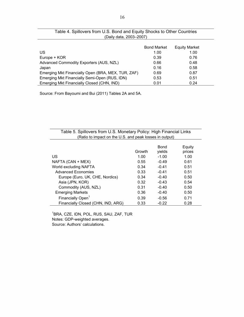
Even in typical times international correlations across financial markets are high. Table 4 reports the average link between a percentage point change in U.S. 10 year bond yields on bond yields and real effective exchange rates in the rest of the world within a single day.8 Pre-crisis the impact on bond yields was estimated at 0.4 percentage points for most advanced economies (slightly higher for commodity producers and lower for Japan), some 0.6 percentage points for financially open emerging markets, and virtually zero for emerging markets with relatively closed financial markets. For all but financially closed emerging markets, this was also accompanied by the expected depreciation of the currency against the dollar.9 In addition, there was no clear difference in the size of the response between NAFTA members and other countries.

Equity returns are generally found to be even more highly correlated than bond returns. For every percentage point that U.S. equity prices rise the typical response of advanced economies is estimated at ½-¾ of a percentage point, for financially open emerging markets the range is one-half to nine-tenths of a percentage point, and for financially closed emerging markets around one-fifth of a percentage point.

For advanced economies and financially open emerging markets these positive estimated financial market spillovers are generally much larger, or even of an opposite sign, from those coming out of the macroeconomic model simulations reported above. The question that naturally arises is what spillovers would look like if the macroeconomic model

7See Bems, Robert and Yi (2011). 8See Bayoumi and Bui (2011) for more details. Similar results are found in Neely (2010). See also Rigobon and Sack (2004). 9Post-crisis patterns for advanced economies are similar, while for emerging markets the tightening of financial conditions comes less through bond yields and more through the exchange rate channel.

10

contained the kind of spillovers on financial markets that we see in the empirical data. This is relatively easy to do. One can replace the fixed, country-specific risk liquidity premium in yield curve (3) with a time-varying liquidity risk premium that includes a large global component.

We reran the simulations with bond market spillovers more like those seen in the pre-crisis data. More precisely, we assume that bond market yields in other advanced economies go up by some 40 percent of the increase in U.S. bond yields. The corresponding ratios for emerging markets with open and closed capital markets are 60 and 20 percent, respectively. The corresponding coefficients for equity markets are 50 percent for advanced economies, and 75 and 25 percent for financially open and closed emerging markets respectively.

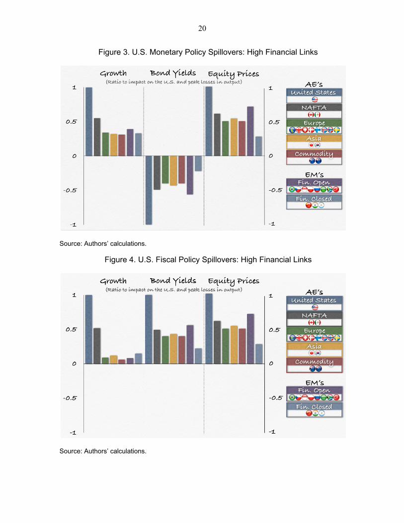
The spillovers from a typical U.S. monetary policy shock are much larger once these bond and equity links are included. Output spillovers from such a simulation are reported in Table 5 and Figure 3. With the fall in U.S. bond market yields ricocheting around the world, now a typical monetary loosening by the United States has spillovers of over one-half on NAFTA countries, compared to one-fifth earlier, and now with a somewhat larger impact on Mexico than Canada (reflecting the larger assumed bond market spillover). The relative impact on other economies leaps by even more. The impact on non-NAFTA economies rises from 7 percent to around one third for advanced economies and financially closed emerging markets, and some 40 percent for financially open emerging markets.

These data correspond much more closely to the types of correlations reported above for the actual data on the global business cycle. They also correspond to the size of spillovers from U.S. shocks estimated using more sophisticated identification techniques (Bayoumi and Bui, 2010).

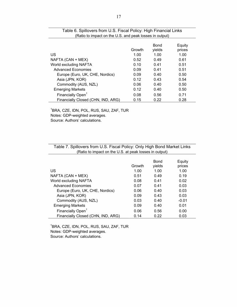
By contrast, the spillovers from a typical fiscal policy shock with higher bond and equity market correlations are quite similar to those reported without these correlations. The impact of a typical fiscal consolidation using these closer bond and equity market links is reported in Table 6 and Figure 4. Overall, the growth spillover coefficients are 52 percent (versus 50 percent without financial market correlations) for NAFTA partners, and 10 percent (versus 9 percent without financial market correlations) for others.

Further analysis demonstrates that the stark difference in results for monetary versus fiscal policy shocks from the modified model comes from the fact that high bond and equity market spillovers reinforce each other in the case of monetary policy but tend to cancel out in the case of fiscal policy. In the case of an expansionary monetary policy, the increase in U.S. output raises equity prices even as the cut in short-term interest rates lowers bond yields. The higher financial market correlations raise foreign equity prices and lower foreign bond yields, thereby massively increasing international growth spillovers compared to the baseline model where foreign bond yields rise and equity prices increase by very little. For fiscal policy, by

11

contrast, the rise in U.S. output raises U.S. and global equity prices but also raises U.S. and global bond yields compared to the baseline model. In the scenario, these two effects approximately cancel out, leading to small net growth spillovers.

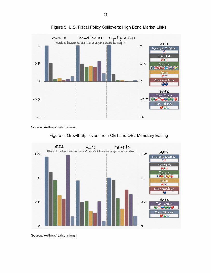
To demonstrate that this is not a universal result, Table 7 and Figure 5 report the results from simulating a U.S. fiscal expansion assuming high bond market spillovers but allowing equity market spillovers to be determined endogenously by the model. Strong bond market spillovers act to lower output in the rest of the world, leading to smaller growth spillovers in all country-groupings except the NAFTA partners, where the benefits from higher trade continue to dominate.

One important conclusion from this analysis is that it is easier to obtain the high growth spillovers seen in the data using monetary/financial shocks than fiscal/real shocks.10 The implication is that the world is more likely dominated by “financial” shocks, in terms of changes in global risk premia, than real ones such as spending. This does not mean that the world is dominated by financial froth—financial shocks may well reflect anticipation of future developments in the real economy. Rather, it implies that the world is dominated by expectations of the future path of economies rather than changes in current behavior.

IV. A PRACTICAL SOLUTION

The previous section has demonstrated that assumptions about financial market spillovers are crucial for estimated international spillovers in large models. In many respects, the situation for an open economy resembles the dilemma faced in deciding upon whether to assume prices are sticky or not in a closed economy model. Assuming sticky wages is difficult to justify theoretically but produces results that correspond much more closely to the actual patterns seen in the data. As a result, almost all policy models assume sticky wages. Similarly, assuming the high asset price correlations across countries seen in the data is difficult to justify on theoretical grounds but produces much more believable international growth spillovers.

There is, however, an important difference between assuming sticky wages and high financial market spillovers, in that financial market reactions can and do vary depending on particular circumstances. In other words, while both sticky wages and high financial correlations can in many respects be assumed to be structural parameters, financial market reactions to specific policy announcements are less predictable. It is common to read in the press that markets reacted well or badly to some policy announcement. By contrast, the same is rarely said about wage setters.

10See also IMF (2012).

12

How can we translate this market commentary into a response that can be used in a macroeconomic model? One viable approach is to use event studies on high frequency data to try and tease out the market reaction to specific events. In the discussion of this potential solution below, we focus on the bond and stock markets, but the approach is equally applicable to other responses. For example, event studies could be used to measure the impact of quantitative easing on exchange rates and commodity prices.

Event studies use market reactions to gauge the impact of a particular policy announcement (say monetary easing) on market prices (say bond yields). Identification is achieved through the timing of the data rather than through more generalized time series techniques (e.g., lags or instruments). In the application we report, daily data are used to measure international bond market spillovers. More precisely, dates of announcements associated with particular policies are identified and reactions of bond markets in different countries are compared.

To be more concrete, key dates associated with announcements of key U.S. monetary and fiscal policies over 2009 and 2010—QE1, QE2, and the 2009 and 2010 fiscal packages—were identified.11 For each of these, the reactions of foreign bond and equity markets in response to changes in U.S. bond and equity markets on these days were compared with the “typical” reactions seen on other days. Any deviation from the typical reaction was then assumed to be the additional, event-specific impact on foreign bond and equity markets—and hence global financial conditions—as a result of that policy. These results are reported in Bayoumi and Bui (2011).

The size of the event window is usually a key issue in event studies, as the impact of a given policy move on the market can materialize slowly over time. In this case, however, there are persuasive reasons for using a short window. Recall that the objective here is not to estimate the impact of QE on U.S. bond yields or equity prices. Rather, given that information, the objective is to identify the knock-on impact from changes in U.S. bond yields/equity prices on foreign bond yields/equity prices. Given that foreign markets are also reacting to local information, using a short window makes it more likely that the measured response will reflect the policy move at hand rather than local noise. In addition, to minimize the potential impact of local noise, estimated spillovers for countries with similar underlying characteristics are averaged—for example, advanced country commodity producers and emerging markets with open capital markets.

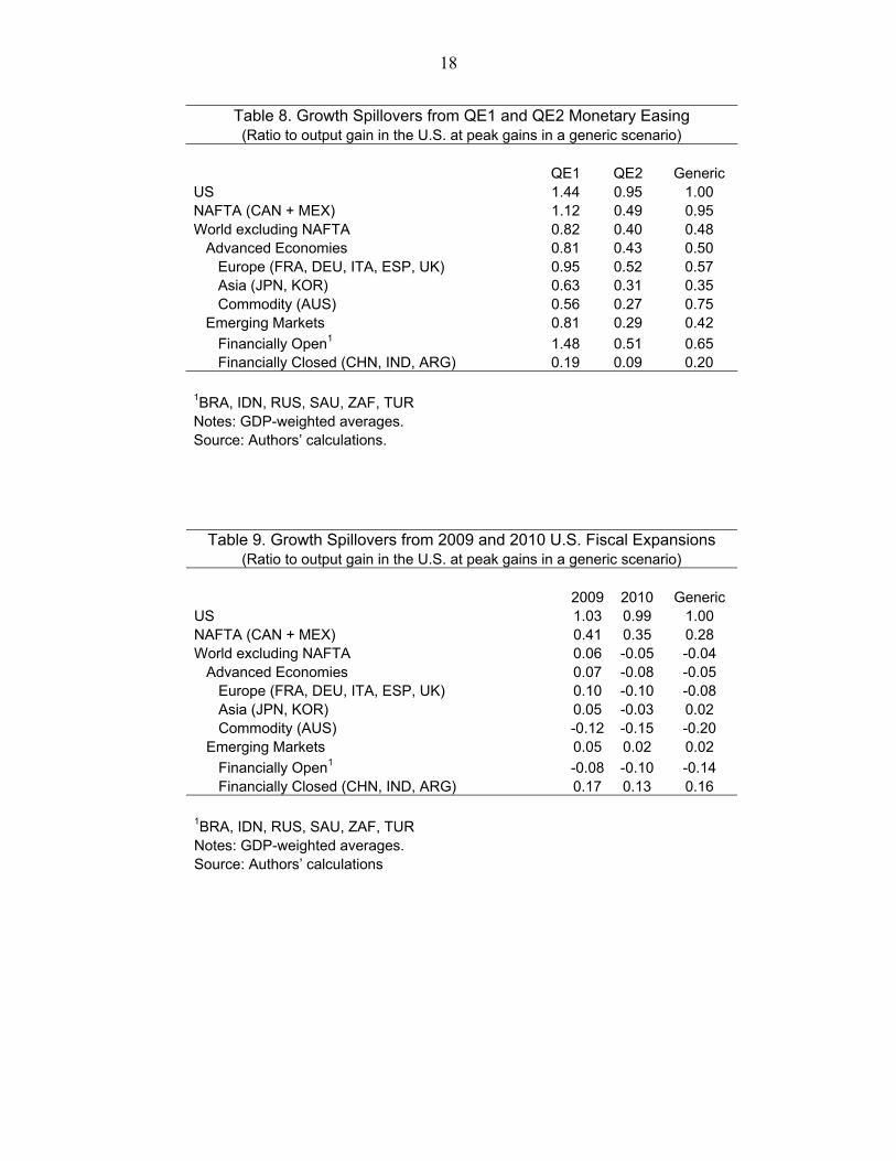
The results from these scenarios, reported in Tables 8 and 9 and Figures 6 and 7, tell an interesting narrative about how financial market responses can vary depending on (perceived) circumstances. Table 8 and Figure 6 show the estimated growth spillovers of

11See IMF (2011).

13

QE1 and QE2 normalized per 1 percentage point reduction in U.S. bond yields. For comparison, the results are also reported for a “baseline” scenario where bond and equity market reactions follow their typical patterns. (These simulations were done on an earlier version of the model from those reported earlier and using a more persistent shock, so the responses to typical patterns are slightly different).12 Because QE1 was estimated to have led to a larger-than-typical fall in foreign bond yields per percentage point reduction in U.S. yields (and also more favorable knock-ons in equity markets), the impact of QE1 on U.S. and foreign growth is estimated to have been significantly more positive than in the baseline simulation. By contrast, QE2 had financial market spillovers that were smaller than was usual, and hence the spillovers were smaller than in the baseline.

This ordering of spillovers corresponds to the usual narrative about QE1 and QE2, namely that QE1 was a major boost to markets at a time when the crisis seemed to be in full swing, while the impact of QE2 was muted since the policy room was regarded as largely used up. Hence, on some basic level, the methodology seems to correspond to the common wisdom about the two policy moves.

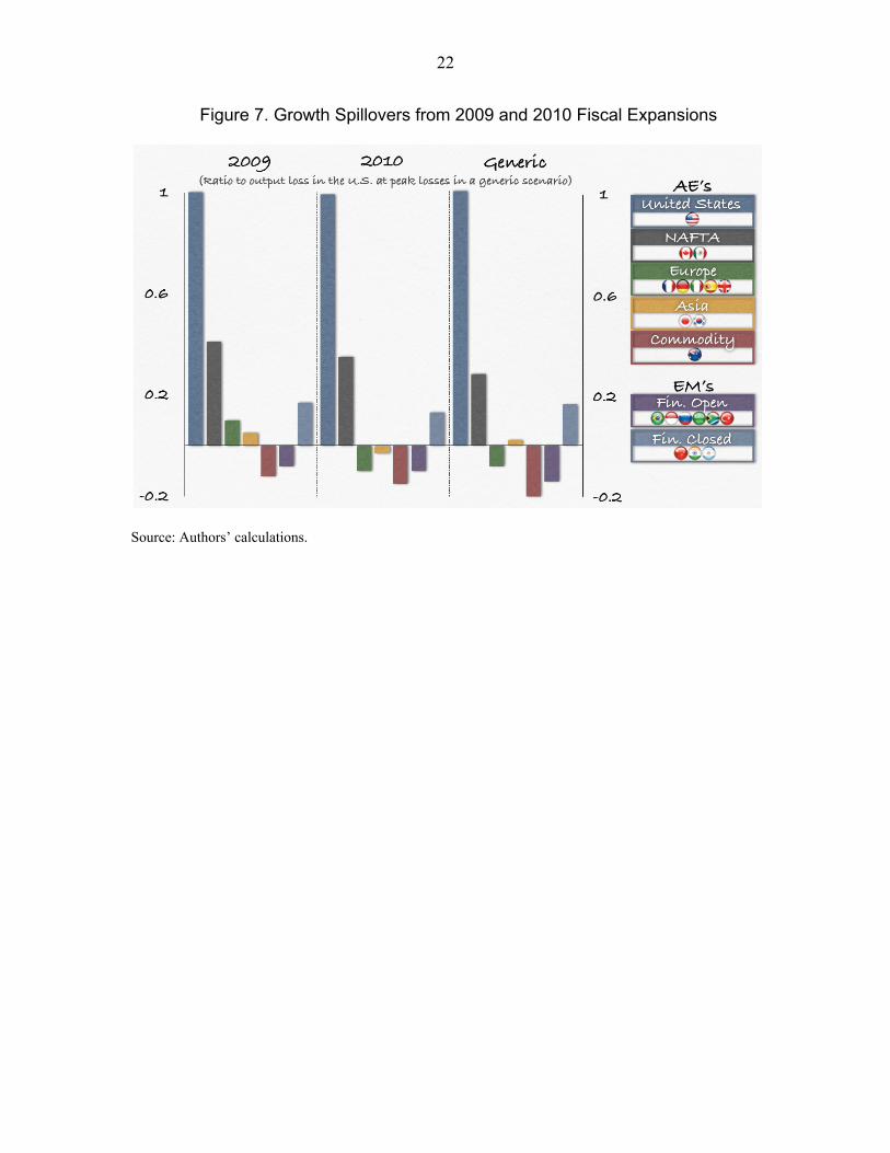
The analysis of the 2009 and 2010 fiscal stimuli, reported in Table 9 and Figure 7, yields a similar lesson.13 Again, the spillovers in global bond and equity markets were much more favorable in 2009 than in 2010, and for similar reasons. In 2009 the U.S. action was seen as a bold move to lower global tail risks, while the 2010 stimulus was seen (wrongly, as it turned out) as questionable given that the global economy was already recovering and U.S. debt was high. As a result, the 2009 stimulus had positive spillovers on many regions of the world, albeit small except for onto NAFTA partners and financially closed emerging markets. By contrast, the 2010 stimulus is estimated to have had negative growth spillovers on all regions except these two, a result more in line with the generic scenario. This illustrates how, in the case of fiscal expansion, financial market responses can lead to quite different spillovers.

V. CONCLUSIONS

This paper has laid out a way of thinking about global growth spillovers. The basic

argument is that the spillovers via financial markets are both potentially larger than through trade channels and much less well understood. The structure of a typical large macroeconomic model generates low correlations of output, bond yields, and (where modeled) equity prices across countries. This does not correspond to the high correlations

12See Vitek (2010). 13The baseline results are again different due to the older model and—in this case in particular—the assumption that the fiscal shock is more persistent which increases the negative impacts on bond markets and causes some growth spillovers to be negative.

14

actually seen in the data. Imposing these financial market correlations produces estimated output spillovers that are much closer to those seen in the data, but we lack a comprehensive model explaining why these international asset price correlations are so high.

In many respects, the situation is similar to the assumption of sticky prices in the domestic sector of macroeconomic models. Again, there is a choice between theoretical rectitude and empirical accuracy. Policy models almost uniformly choose sticky wages and empirical accuracy. The same is likely to be true of policy models when it comes to financial market correlations and the associated international growth spillovers.

But in the case of financial markets there is a further complication. Financial markets are forward-looking, and so their response is not mechanical but depends on the situation. This explains the myriad of market analysts employed in the financial industry to assess and predict reactions. This paper argues that an attractive option is to use event studies to calibrate market reactions to particular policy announcements. Using U.S. monetary and fiscal policy announcements in 2009 and 2010, this paper argues that such a procedure can produce results that are plausible and event-specific.

15

Table 1. Spillovers from U.S. Monetary Policy: Typical Model

(Ratio to impact on the U.S. and peak losses in output)

GrowthBond yields

Equity prices

US 1.00 -1.00 1.00 Other NAFTA (CAN + MEX) 0.22 0.67 0.18 World excluding NAFTA 0.07 0.20 0.06 Advanced Economies 0.07 0.20 0.07 Europe (Euro, UK, CHE, Nordics) 0.09 0.21 0.08 Asia (JPN, KOR) 0.04 0.18 0.04 Commodity (AUS, NZL) 0.05 0.11 0.03 Emerging Markets 0.08 0.22 0.05

Financially Open1 0.05 0.06 0.03 Financially Closed (CHN, IND, ARG) 0.11 0.40 0.08

1BRA, CZE, IDN, POL, RUS, SAU, ZAF, TUR Notes: GDP-weighted averages. Source: Authors’ calculations.

Table 2. Spillovers from U.S. Fiscal Policy: Typical Model (Ratio to impact on the U.S. and peak losses in output)

GrowthBond yields

Equity prices

US 1.00 1.00 1.00 NAFTA (CAN + MEX) 0.50 0.50 0.18 World excluding NAFTA 0.09 0.08 0.03 Advanced Economies 0.08 0.10 0.04 Europe (Euro, UK, CHE, Nordics) 0.08 0.10 0.03 Asia (JPN, KOR) 0.11 0.10 0.04 Commodity (AUS, NZL) 0.05 0.01 0.00 Emerging Markets 0.11 0.01 0.02

Financially Open1 0.07 0.07 0.01 Financially Closed (CHN, IND, ARG) 0.15 -0.06 0.03 1BRA, CZE, IDN, POL, RUS, SAU, ZAF, TUR

Notes: GDP-weighted averages.

Source: Authors’ calculations.

Table 3. Correlations of Quarterly Output Growth, 1980–2012

  EA UK US

EA 1

UK 0.53 1

US 0.44 0.48 1Source: Authors’ calculations.

16

Table 4. Spillovers from U.S. Bond and Equity Shocks to Other Countries (Daily data, 2003–2007)

Bond Market Equity Market US 1.00 1.00 Europe + KOR 0.39 0.76 Advanced Commodity Exporters (AUS, NZL) 0.66 0.48 Japan 0.16 0.58 Emerging Mkt Financially Open (BRA, MEX, TUR, ZAF) 0.69 0.87 Emerging Mkt Financially Semi-Open (RUS, IDN) 0.53 0.51 Emerging Mkt Financially Closed (CHN, IND) 0.01 0.24 Source: From Bayoumi and Bui (2011) Tables 2A and 5A.

Table 5. Spillovers from U.S. Monetary Policy: High Financial Links (Ratio to impact on the U.S. and peak losses in output)

GrowthBond yields

Equity prices

US 1.00 -1.00 1.00 NAFTA (CAN + MEX) 0.55 -0.49 0.61 World excluding NAFTA 0.34 -0.41 0.51 Advanced Economies 0.33 -0.41 0.51 Europe (Euro, UK, CHE, Nordics) 0.34 -0.40 0.50 Asia (JPN, KOR) 0.32 -0.43 0.54 Commodity (AUS, NZL) 0.31 -0.40 0.50 Emerging Markets 0.36 -0.40 0.50

Financially Open1 0.39 -0.56 0.71 Financially Closed (CHN, IND, ARG) 0.33 -0.22 0.28 1BRA, CZE, IDN, POL, RUS, SAU, ZAF, TUR Notes: GDP-weighted averages. Source: Authors’ calculations.

17

Table 6. Spillovers from U.S. Fiscal Policy: High Financial Links (Ratio to impact on the U.S. and peak losses in output)

GrowthBond yields

Equity prices

US 1.00 1.00 1.00 NAFTA (CAN + MEX) 0.52 0.49 0.61 World excluding NAFTA 0.10 0.41 0.51 Advanced Economies 0.09 0.41 0.51 Europe (Euro, UK, CHE, Nordics) 0.09 0.40 0.50 Asia (JPN, KOR) 0.12 0.43 0.54 Commodity (AUS, NZL) 0.06 0.40 0.50 Emerging Markets 0.12 0.40 0.50

Financially Open1 0.08 0.56 0.71 Financially Closed (CHN, IND, ARG) 0.15 0.22 0.28 1BRA, CZE, IDN, POL, RUS, SAU, ZAF, TUR Notes: GDP-weighted averages. Source: Authors’ calculations.

Table 7. Spillovers from U.S. Fiscal Policy: Only High Bond Market Links (Ratio to impact on the U.S. at peak losses in output)

GrowthBond yields

Equity prices

US 1.00 1.00 1.00 NAFTA (CAN + MEX) 0.51 0.49 0.19 World excluding NAFTA 0.08 0.41 0.02 Advanced Economies 0.07 0.41 0.03 Europe (Euro, UK, CHE, Nordics) 0.06 0.40 0.03 Asia (JPN, KOR) 0.09 0.43 0.03 Commodity (AUS, NZL) 0.03 0.40 -0.01 Emerging Markets 0.09 0.40 0.01

Financially Open1 0.06 0.56 0.00 Financially Closed (CHN, IND, ARG) 0.14 0.22 0.03 1BRA, CZE, IDN, POL, RUS, SAU, ZAF, TUR Notes: GDP-weighted averages. Source: Authors’ calculations.

18

Table 8. Growth Spillovers from QE1 and QE2 Monetary Easing (Ratio to output gain in the U.S. at peak gains in a generic scenario)

QE1 QE2 Generic US 1.44 0.95 1.00 NAFTA (CAN + MEX) 1.12 0.49 0.95 World excluding NAFTA 0.82 0.40 0.48 Advanced Economies 0.81 0.43 0.50 Europe (FRA, DEU, ITA, ESP, UK) 0.95 0.52 0.57 Asia (JPN, KOR) 0.63 0.31 0.35 Commodity (AUS) 0.56 0.27 0.75 Emerging Markets 0.81 0.29 0.42

Financially Open1 1.48 0.51 0.65 Financially Closed (CHN, IND, ARG) 0.19 0.09 0.20 1BRA, IDN, RUS, SAU, ZAF, TUR Notes: GDP-weighted averages. Source: Authors’ calculations.

Table 9. Growth Spillovers from 2009 and 2010 U.S. Fiscal Expansions (Ratio to output gain in the U.S. at peak gains in a generic scenario)

2009 2010 Generic US 1.03 0.99 1.00 NAFTA (CAN + MEX) 0.41 0.35 0.28 World excluding NAFTA 0.06 -0.05 -0.04 Advanced Economies 0.07 -0.08 -0.05 Europe (FRA, DEU, ITA, ESP, UK) 0.10 -0.10 -0.08 Asia (JPN, KOR) 0.05 -0.03 0.02 Commodity (AUS) -0.12 -0.15 -0.20 Emerging Markets 0.05 0.02 0.02

Financially Open1 -0.08 -0.10 -0.14 Financially Closed (CHN, IND, ARG) 0.17 0.13 0.16 1BRA, IDN, RUS, SAU, ZAF, TUR Notes: GDP-weighted averages. Source: Authors’ calculations

19

Figure 1. U.S. Monetary Policy Spillovers: Typical Model

Source: Authors’ calculations.

Figure 2. U.S. Fiscal Policy Spillovers: Typical Model

Source: Authors’ calculations.

20

Figure 3. U.S. Monetary Policy Spillovers: High Financial Links

Source: Authors’ calculations.

Figure 4. U.S. Fiscal Policy Spillovers: High Financial Links

Source: Authors’ calculations.

21

Figure 5. U.S. Fiscal Policy Spillovers: High Bond Market Links

Source: Authors’ calculations.

Figure 6. Growth Spillovers from QE1 and QE2 Monetary Easing

Source: Authors’ calculations.

22

Figure 7. Growth Spillovers from 2009 and 2010 Fiscal Expansions

Source: Authors’ calculations.

23

References

Bayoumi, T. and T. Bui, 2010, “Deconstructing the International Business Cycle: Why Does

A U.S. Sneeze Give the Rest of the World a Cold?” IMF Working Paper 10/239 (Washington: International Monetary Fund).

Bayoumi, T. and T. Bui, 2011, “Unforeseen Events Wait Lurking: Estimating Policy

Spillovers from U.S. to Foreign Asset Prices,” Working Paper 11/183 (Washington: International Monetary Fund).

Bayoumi, T. and A. Swiston, 2007, “Foreign Entanglements: Estimating the Source and Size

of Spillovers across Industrial Countries,” Working Paper 07/182 (Washington: International Monetary Fund).

Bems, R., C. Robert, and K. Yi, 2011, “Vertical Linkages and the Collapse of Global Trade,”

American Economic Review Papers and Proceedings, Vol. 101:3, pp108–12. Bernanke, B., V. Reinhart, and B. Sack, 2004, “Monetary Policy Alternatives at the Zero

Bound: An Empirical Assessment,” Brookings Papers on Economic Activity 2004 No. 2, pp 1–100.

Bordo, M, and T. Helbling, 2004, “Have National Business Cycles Become More

Synchronized?” In Siebert, H. (ed.), Macroeconomic Policies in the World Economy (Berlin-Heidelberg: Springer Verlag).

Brunnermeier, M., T. Eisenbach, and Y. Sannikov, 2012, “Macroeconomics with Financial

Frictions: A Survey,” unpublished manuscript. Bryant, Ralph C., and others, eds., 1988, Empirical Macroeconomics for Interdependent

Economies (Washington: Brookings Institution). Gürkaynak, R., B. Sack and E. Swanson, 2005, “So Actions Speak Louder than Words? The

Response of Asset Prices to Monetary Policy Actions and Statements,” International Journal of Central Banking, Vol. 1, No. 1, pp 55–93.

International Monetary Fund, 2011, United States: Spillover Report—2011 Article IV

Consultation, IMF Country Report No. 11/203 (Washington). International Monetary Fund, 2012, 2012 Spillover Report (Washington). Available on the

Internet: http://www.imf.org/external/np/pp/eng/2012/070912.pdf

24

Kose, M., C. Otrok, and C. Whiteman, 2003, “International Business Cycles: World, Region, and Country-Specific Factors,” American Economic Review, Vol. 93, (September), pp. 1216–39.

Montford, A, J-P Renne, R. Ruffer, and G. Vitale, 2003, “Is Economic Activity in the G7

Synchronized? Common Shocks versus Spillover Effects,” CEPR Discussion Paper No. 4119 (London: Centre for Economic Policy Research).

Neely, C.J., 2010, “The Large-Scale Asset Purchases Had Large International Effects,”

Working Paper 2010–018C (St. Louis: Federal Reserve Bank of St. Louis). Available on the Internet: http://research.stlouisfed.org/wp/more/2010-018/

Rigobon, R. and B. Sack, 2004, “The Impact of Monetary Policy on Asset Prices,” Journal of

Monetary Economics, Vol. 51, pp. 1553–75. Stock, J., and M. Watson, 2005, “Understanding Changes in International Business Cycle

Dynamics,” Journal of the European Economic Association, Vol. 3 (September), pp. 968–1006.

Swiston, A., 2007, “Where Have the Monetary Surprises Gone? The Effects of FOMC

Statements,” IMF Working Paper 07/185 (Washington: International Monetary Fund).

Vitek, F., 2010, “Monetary Policy Analysis and Forecasting in the Group of Twenty: A Panel

Unobserved Components Approach,” IMF Working Paper 10/152 (Washington: International Monetary Fund).

Vitek, F., 2012, “Policy Analysis and Forecasting in the World Economy: A Panel

Unobserved Components Approach,” IMF Working Paper 12/149 (Washington: International Monetary Fund).