Macro Fiber Composite Actuated Unmanned Air Vehicles: Design, … · 2020-01-22 · Macro Fiber Composite Actuated Unmanned Air Vehicles: Design, Development, and Testing Onur Bilgen

Macro Fiber Composite Actuated Unmanned Air

Vehicles: Design, Development, and Testing

by

Onur Bilgen

Thesis submitted to the faculty of the Virginia Polytechnic Institute and State University

in partial fulfillment of the requirements for the degree of

Master of Science

in

Mechanical Engineering

A. J. Kurdila, Chairman D. J. Inman, Co-Chair

K. Kochersberger, Member A. L. Wicks, Member

May 10, 2007

Blacksburg, Virginia

Key Words: micro air vehicles, Macro Fiber Composite, morphing wing, composite

materials, unimorph structure

© Onur Bilgen, 2007

Macro Fiber Composite Actuated Unmanned Air

Vehicles: Design, Development, and Testing

Onur Bilgen

Abstract

The design and implementation of a morphing unmanned aircraft using smart

materials is presented. Articulated lifting surfaces and articulated wing sections actuated

by servos are difficult to instrument and fabricate in a repeatable fashion on thin,

composite-wing micro-air-vehicles. Assembly is complex and time consuming. A type

of piezoceramic composite actuator commonly known as Macro Fiber Composite (MFC)

is used for wing morphing. The actuation capability of this actuator on

fiberglass unimorph was modeled by the Rayleigh-Ritz method and quantified by

experimentation. Wind tunnel tests were performed to compare conventional trailing

edge control surface effectiveness to an MFC actuated wing section. The

continuous surface of the MFC actuated composite airfoil produced lower drag and wider

actuation bandwidth. The MFC actuators were implemented on a 0.76 m wingspan

aircraft. The remotely piloted experimental vehicle was flown using two MFC patches in

an elevator/aileron (elevon) configuration. Preliminary testing has proven the stability

and control of the design. Flight tests were performed to quantify roll control using the

actuators. Force and moment coefficients were measured in a low-speed, open section

wind tunnel, and the database of aerodynamic derivatives were used to analyze control

response.

Dedication

to my parents,

Deniz and Ahmet Saim Bilgen…

iii

Acknowledgements

First, I would like to thank Dr. Kevin Kochersberger for his support and for the

direction he provided for the research. Without his leadership, none of this work would

have been possible.

Thanks to Dr. Daniel J. Inman and Dr. Andrew J. Kurdila for serving as my

advisors, offering ideas, and sharing their expertise in the research.

Wind tunnel tests presented in Chapter 3 were possible with the help of Dr. Karen

A. Thole and the graduate students at the Experimental and Computational Convection

Laboratory (ExCCL).

I would like to thank Rodney Brown for his dedication to fly the aircraft. His pilot

skills and patience thru the countless flight attempts made the flight tests possible.

Thanks to Dr. William J. Devenport at the Aerospace and Ocean Engineering

Department. The wind tunnel tests on the aircraft were done with his kind assistance.

I would like to acknowledge the help and support from my colleagues at the

Institute for Advanced Learning and Research (IALR) in Danville, VA. Thanks to the

graduate students at the Center for Intelligent Material Systems and Structures (CIMSS)

for sharing their ideas and expertise in theoretical, computational, and experimental

subjects.

Furthermore, I would like to thank the CIMSS and the Joint Unmanned Systems

Test, Experimentation and Research (JOUSTER) program for funding the research.

iv

Table of Contents

Abstract.............................................................................................................................. ii

Dedication ......................................................................................................................... iii

Acknowledgements .......................................................................................................... iv

List of Figures................................................................................................................. viii

List of Tables ................................................................................................................... xii

Chapter 1: Introduction and Background .................................................................... 1

1.1 Motivation............................................................................................................ 1

1.2 Background and Literature Review ..................................................................... 2

1.2.1 Micro Air Vehicles .................................................................................. 2

1.2.2 Morphing Wing Aircraft .......................................................................... 3

1.2.3 Smart Materials........................................................................................ 6

1.2.4 The Macro Fiber Composite .................................................................... 8

1.3 Objectives .......................................................................................................... 10

1.4 Outline of the Thesis.......................................................................................... 10

Chapter 2: Modeling and Experimentation of MFC Actuated Laminates .............. 12

2.1 Classical Lamination Theory ............................................................................. 12

2.2 Strain – Displacement Relations of the Unimorph ............................................ 14

2.3 Potential Energy Calculations............................................................................ 16

2.3.1 Host Laminate Potential Energy ............................................................ 16

2.3.2 Actuator Potential Energy without Applied Voltage ............................. 17

2.3.3 Total Potential Energy of the Actuator - Host (0 Volts)........................ 18

2.3.4 Actuator Potential Energy with Applied Voltage .................................. 19

v

2.3.5 Total Potential Energy of the Actuator - Host with Applied Voltage.... 21

2.4 Prediction of Displacement Fields ..................................................................... 21

2.5 Static Deflection Tests and Comparison to Model ............................................ 22

Chapter 3: Wind Tunnel Experimentation on a Morphing Airfoil .......................... 28

3.1 Wind Tunnel ...................................................................................................... 30

3.2 Mechanical Balance ........................................................................................... 33

3.3 Calculating Lift and Drag Coefficients.............................................................. 34

3.4 Wind Tunnel Test Results.................................................................................. 35

Chapter 4: Micro Air Vehicle Design and Fabrication.............................................. 42

4.1 Overall Aircraft and Wing Design..................................................................... 42

4.2 Main Frame and Fuselage.................................................................................. 46

4.3 Electronics.......................................................................................................... 48

4.3.1 MFC Power Electronics......................................................................... 48

4.3.2 Power Booster Circuit............................................................................ 48

4.3.3 Battery and Propulsion System.............................................................. 49

4.3.4 Transmitter and Receiver....................................................................... 50

4.3.5 Layout of the Electronics ....................................................................... 50

4.4 Overall Specifications of the Aircraft ................................................................ 52

Chapter 5: Wind Tunnel and Flight Tests of the Aircraft......................................... 54

5.1 Wind Tunnel Experimentation of the Aircraft................................................... 54

5.1.1 Lift, Drag and Moment Calculations ..................................................... 56

5.1.2 Uncertainty Analysis.............................................................................. 58

5.1.3 Wind Tunnel Test Results...................................................................... 59

5.1.4 Dynamic Response Results.................................................................... 64

vi

5.2 Flight Tests......................................................................................................... 65

Chapter 6: Conclusions and Future Work.................................................................. 69

6.1 Brief Summary of Results.................................................................................. 69

6.2 Publications........................................................................................................ 70

6.3 Future Work ....................................................................................................... 71

References........................................................................................................................ 72

Appendix A: Stiffness Properties of the MFC......................................................... 75

Appendix B: Mechanical Balance ............................................................................ 86

Appendix C: Flow Speed Adjustments .................................................................... 92

Appendix D: Additional Information on the Aircraft............................................ 94

Appendix E: Additional Results from Wind Tunnel Tests on the Aircraft ......... 99

Vita ................................................................................................................................. 102

vii

List of Figures

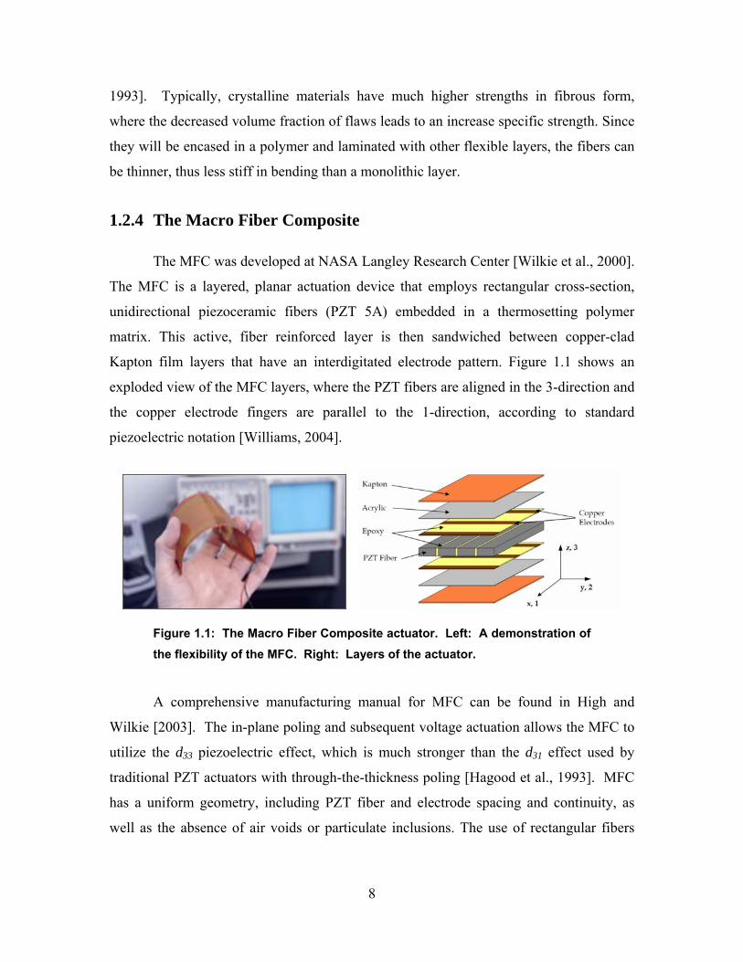
Figure 1.1: The Macro Fiber Composite actuator. Left: A demonstration of the flexibility of the MFC. Right: Layers of the actuator. ..................................8

Figure 2.1: Layers of the MFC actuator. [Williams, 2004] .............................................13

Figure 2.2: Side and top view of the host-laminate and MFC actuator (unimorph) structure.........................................................................................................14

Figure 2.3: Midsurface deflection of MFC actuated laminate..........................................22

Figure 2.4: Illustration of the unimorph structure. Clamped section is not shown..........23

Figure 2.5: Experiment setup for the displacement measurement of the unimorph actuator..........................................................................................................24

Figure 2.6: Tip deflection of the unimorph structure with applied voltage. .....................24

Figure 2.7: Deflection vs. host thickness plot for the calibration specimen. ....................26

Figure 2.8: Deflection vs. host laminate thickness plot for all tested specimens. ............26

Figure 3.1: Left: CAD model of the mold. Middle: Tool path for milling machine. Right: Milling simulation running on Unigraphics NX3. ...........28

Figure 3.2: CNC machined mold and cured fiberglass / epoxy composite. Two 10 cm X 10 cm wing sections were cut from the blank composite. ..................29

Figure 3.3: MFC actuated fiberglass wing section in the wind tunnel. Leading edge is on the left. White rectangles are the reflective tape pieces for displacement measurements..........................................................................29

Figure 3.4: Flapped fiberglass wing section. The safety wire link, used to adjust the flap angle, is shown in the oval...............................................................30

Figure 3.5: Wind tunnel setup and the test equipment......................................................30

Figure 3.6: Wing section suspended in the tunnel. Vibrometer is aimed at the variable camber airfoil in the test section. ....................................................31

Figure 3.7: Illustration of the wind tunnel setup. The bolts that secure the separator panels to the ceiling and the floor of the test section are not shown. ...........................................................................................................31

Figure 3.8: Picture of the test section. Airflow is out of the page. ...................................32

Figure 3.9: CAD model of the mechanical wind tunnel balance. The setup shown measures lift force.........................................................................................33

Figure 3.10: Top and front view of the mechanical beam balance...................................34

Figure 3.11: CL comparison plot at 16.5 m/s for morphing and flapped fiberglass wing...............................................................................................................36

viii

Figure 3.12: CD comparison plot at 16.5 m/s for morphing and flapped fiberglass wing...............................................................................................................36

Figure 3.13: L/D comparison plot at 16.5 m/s for morphing and flapped fiberglass wing. .............................................................................................37

Figure 3.14: CL comparison plot at 11.9 m/s for morphing and flapped fiberglass wing...............................................................................................................37

Figure 3.15: CD comparison plot at 11.9 m/s for morphing and flapped fiberglass wing...............................................................................................................38

Figure 3.16: L/D comparison plot at 11.9 m/s for morphing and flapped fiberglass wing. .............................................................................................38

Figure 3.17: Mid-span deflection plots for MFC actuated test wing at the indicated voltage level and angle of attack. Voltage and camber are abbreviated as V and C respectively. “Flow” given at each subplot indicates the measured air speed. Rec=1.17x105..........................................40

Figure 3.18: Comparison of lift and drag coefficients of 4% cambered 2D airfoil. .........41

Figure 4.1: Airfoil profile at the root of the wing. Leading edge is on the left. ...............42

Figure 4.2. Initial MAV design.........................................................................................43

Figure 4.3: Final design of the wings. The camber of the reflex at the trailing-edge is constant along the span.....................................................................44

Figure 4.4: Illustration of fiberglass layer change along the span of the wing. MFC actuator is applied on the single layer section. ....................................44

Figure 4.5: Right and left wings and molds......................................................................45

Figure 4.6: Left: Trimmed wing sections. Right: Root chord of both wings..................45

Figure 4.7: Fiberglass composite wing ready to be mounted on the aircraft. 380 mm span and 150 mm chord. Leading edge is shown on the top. ................46

Figure 4.8: Illustration of main frame and fuselage/electronics bay. Left wing is not shown. .....................................................................................................47

Figure 4.9: Main frame. Clevis links are used to adjust dihedral. ...................................47

Figure 4.10: Power booster circuit. Circuit weighs about 22 grams................................49

Figure 4.11: Illustration of the MFC power electronics. ..................................................49

Figure 4.12: Placement of electronics in the fuselage / electronics bay. ..........................51

Figure 4.13: Assembled electronics and the motor system. MFC patches (not shown) are connected to the output of the DC-DC converters (left side of the picture). .......................................................................................51

Figure 4.14: Fabricated micro air vehicle. Tail weight used to trim pitch is not shown. ...........................................................................................................53

Figure 4.15: Micro air vehicle during its first flight on Feb 28, 2007. .............................53

ix

Figure 5.1: Open section wind tunnel setup. Airflow is from left to right. Pitot tube is on the top left corner of the picture. ..................................................54

Figure 5.2: Test aircraft on the wind tunnel sting balance................................................55

Figure 5.3: Illustration of the coordinate system for aircraft and the sting balance. Right hand rule is used to define roll axis which is labeled as Mx...............56

Figure 5.4: Wing tip deflection at the indicated voltage level. Measurements were taken at wind-off condition. Voltage and camber are abbreviated as V and C respectively.....................................................................................57

Figure 5.5: Lift coefficient comparison of symmetrically actuated wings to non-actuated case at 10.3 m/s. Rec=9.8*104. ......................................................60

Figure 5.6: Drag coefficient comparison of symmetrically actuated wings to non-actuated case at 10.3 m/s. Rec=9.8*104. ......................................................61

Figure 5.7: Lift / Drag comparison of symmetrically actuated wings to non-actuated case at 10.3 m/s. Rec=9.8*104. ......................................................61

Figure 5.8. Lift and drag response to applied voltage represented in time history plots for AOA=4.4 degrees at 10.3 m/s. Rec=9.8*104. Relatively small increase in drag due to actuation is observed......................................62

Figure 5.9: Roll moment response to applied voltage represented in time history plots for AOA=4.4 degrees at 10.3 m/s. Rec=9.8*104. ................................63

Figure 5.10: Execution of roll maneuver. Time stamp is located on the bottom left corner of the frames. Video link is embedded in the figure. ..................67

Figure A.1: Illustration of normal and shear stresses applied on an element. [Jones, 1999] .................................................................................................75

Figure A.2: Components of the compliance matrix for an anisotropic material. .............76

Figure A.3: Coordinate system for defining stress in the lamina. ....................................77

Figure A.4: Transverse cross section of the MFC actuator. PZT fiber runs normal to the page. [Wilkie, 2000] ...........................................................................78

Figure A.5: Longitudinal photomicrograph of the MFC actuator. Copper electrode is normal to the page. [Wilkie, 2000]...........................................79

Figure A.6: Coordinate system for a two dimensional rotation........................................81

Figure A.7: Assembly of the individual lamina along the thickness. Midsurface (z4=0) is shown with dashed line. .................................................................83

Figure A.8: Boundary of each layer. The total thickness is 0.32 mm..............................83

Figure B.1: Illustration of the mechanical wind tunnel balance. ......................................86

Figure B.2: Calibration of the mechanical balance. Wind tunnel is off. .........................88

Figure B.3: Forces acting on the balance in lift measurement configuration. Airflow is out of the page. ............................................................................89

x

Figure B.4: Forces acting on the balance in drag measurement configuration. Airflow is in-plane with the page, from right to left.....................................90

Figure C.1: Boundary-layer thickness definition. [Fox, 2004]........................................92

Figure D.1: CAD model of the molds for left and right wing. .........................................94

Figure D.2: Tool-path simulation running in Unigraphics NX3.......................................94

Figure D.3: Calibration of voltage divider circuit. ...........................................................95

Figure D.4: DC-DC converter response to input voltage. ................................................96

Figure D.5: Power consumption of booster circuit and the DC-DC converter.................96

Figure D.6: DC-DC converter output voltage vs. stick position.......................................97

Figure D.7: Power consumption of all electronics............................................................97

Figure E.1: Lift force response to applied voltage represented in time history plots for all AOAs (α) tested. Rec=9.8*104..................................................99

Figure E.2: Drag force response to applied voltage represented in time history plots for all AOAs (α) tested. Rec=9.8*104................................................100

Figure E.3: Roll moment response of left wing to applied voltage represented in time history plots for all AOAs (α) tested. Rec=9.8*104. ..........................101

Figure E.4: Roll moment response of right wing to applied voltage represented in time history plots for all AOAs (α) tested. Rec=9.8*104. ..........................101

xi

List of Tables

Table 1.1: Effects of increase / decrease of geometric wing parameters on aircraft performance. [Jha and Kudva, 2004]..............................................................4

Table 1.2: Selected properties for common piezoceramic materials. The boundary condition superscripts are: T = constant stress; E = constant field. [Wilkie, 2006] .................................................................................................7

Table 2.1: General properties of the tested unimorph structures. Note that Thickness indicated is for the host laminate only.........................................23

Table 2.2: Parameters used in the Rayleigh-Ritz model. MFC properties were used from the specification sheet instead of the CLT prediction..................25

Table 4.1: Receiver channel setup. ...................................................................................50

Table 4.2: Aircraft specifications......................................................................................52

Table 5.1: Absolute uncertainties for force and moment measurements and corresponding coefficients. ...........................................................................59

Table A.1: Properties for each lamina in the MFC actuator. ............................................83

xii

Chapter 1: Introduction and Background

1.1 Motivation

Design, manufacturing, and the control of micro air vehicles (MAVs) in unsteady

aerodynamic loading remain an active area of interest to researchers. MAVs are a class of

aircraft that are small and inexpensive. They can be used for missions where larger

vehicles are not practical, such as low altitude battlefield, urban, and wildlife

surveillance. The fabrication of MAVs has become more feasible with the decreased

size and weight of sensors, video, communication devices, and many other electronic

subsystems. However, it is known that articulated lifting surfaces and articulated wing

sections actuated by servos are difficult to instrument and fabricate in a repeatable

fashion on thin, composite wing MAVs. Assembly of the vehicle is complex and time

consuming. Solid-state actuators could be employed to address these issues.

The past few decades have seen the development and integration of active

materials into a variety of host structures as a superior means of measuring and

controlling its behavior [Williams, 2004]. Piezoceramics remain the most widely used

“smart” or active material because they offer high actuation authority and sensing over a

wide range of frequencies. Specifically, piezoceramic materials have been extensively

studied and employed in aerospace structures by performing shape and flow control.

Macro Fiber Composite (MFC) is a type of piezoceramic material that offers structural

flexibility and high actuation authority.

A common disadvantage with piezoceramic actuators and with the MFC actuator

is that they require high voltage input. An MFC actuator could require up to 2 kV and

some active materials may require up to 10 kV. In contrast, the current drain is usually

low creating reasonable power consumption. The high voltage demand requires

additional amplifiers and electronic circuits to be included in the system. Due to the

weight of the electronic logistical systems that come along with the active material, these

actuators have been used mostly in large vehicles or in the laboratory environment. With

1

the recent development in the electronic systems, active materials become feasible in

small platforms such as MAVs.

Smart materials can be employed for control in thin, composite-wing MAVs.

There are several benefits of using camber control via solid-state active materials over the

trailing edge control using conventional control surfaces. First, the low Reynolds

Number flow regime can result in flow separation that reduces the effectiveness of a

trailing edge control surface. Second, power-limited aircraft such as MAVs cannot afford

to lose energy through control surface drag. Finally, the opportunity for flow control is

inherent in the active material due to its direct effect on circulation and high operating

bandwidth.

1.2 Background and Literature Review

1.2.1 Micro Air Vehicles

Micro air vehicles represent a new challenge for aerodynamics, propulsion and

control design. Typical MAV missions are projected to be flown either by inexperienced

operators or via autonomous control. This requires robust flying characteristics. It is well

known that during flight in the Reynolds Number range between 10,000 and 100,000,

flow separation around an airfoil can lead to sudden increases in drag and loss of

efficiency. The effects of flow separation can be seen in nature where large species soar

for extended periods of time while small birds have to flap vigorously to remain airborne.

The Reynolds Numbers of the larger species are well above 100,000 whereas

hummingbirds fly at below 10,000 if they attempt to soar [Ifju et al., 2001].

The researchers at the University of Florida have developed a series of MAVs that

incorporate a unique, thin, reflexed, flexible wing design [Waszak et al., 2001, Ifju et al.,

2002]. The wings are constructed of a carbon fiber skeleton and a thin flexible latex

membrane. There is some evidence that the flexible wing design reduces the adverse

effects of gusty wind conditions and unsteady aerodynamics, exhibits desirable flight

stability, and enhances structural durability.

2

There have been numerous experimental and analytical studies on flexible wing

MAVs. Albertani et al. [2004] investigated the effects of a propeller on the aerodynamic

characteristics of MAVs and the coupling with the wing flexibility in steady conditions.

The MAV was placed in a wind tunnel and subjected to different flow conditions and

different motor speeds. Data were gathered through a sting balance and two cameras for

stereovision and image correlation. The test data provided a detailed account of

aerodynamics as they relate to the propeller effects and to the structural deformations,

namely the wing flexibility.

Garcia et al. [2003] investigated the use of a morphing method to provide control

authority. A torque tube actuated by servos twisted or curled the flexible wing. Flight

tests show that wing twisting or curling was a good strategy to command roll maneuvers.

The vehicles were easy to fly and were suitable for autopilot control.

The aerodynamic characteristics of isolated MAV wings and complete aircraft are

considered a good base study for general aerodynamic considerations and a necessary

step for a sound MAV wing design [Torres, 2002]. Prandtl [1921] and Hoerner [1975]

and many others studied the general aerodynamic effects of propellers on the wing and

the aircraft. Barlow, Rae and Pope [1999] established standard wind tunnel testing

techniques.

1.2.2 Morphing Wing Aircraft

A morphing aircraft changes its configuration to maximize its performance in

significantly different flight environments. Wing morphing has been of interest to

researchers because wings directly affect flight performance. The Wright Brothers’ first

controlled, powered, heavier-than-air flight in 1903 was primarily a success due to the

application of the morphing concept.

The Wright’s were convinced that control of the flying machine was the key

challenge. They decided that a “good” way for flying was to "bank" or "lean" into the

turn just like a bird, and just like a person riding a bicycle. They puzzled over how to

achieve this effect with man-made wings and eventually discovered wing-warping when

Wilbur twisted a long inner tube box at their bicycle shop [Wright].

3

The early mechanical method of morphing led to the current search for a

morphing technique with maximum efficiency. Morphing is necessary for several

reasons. A long-endurance aircraft can loiter over a target for an extended time because it

utilizes a high aspect ratio, unswept wing. However, this choice of planform is in direct

conflict with the design of a high speed aircraft requiring a low aspect ratio, swept wing

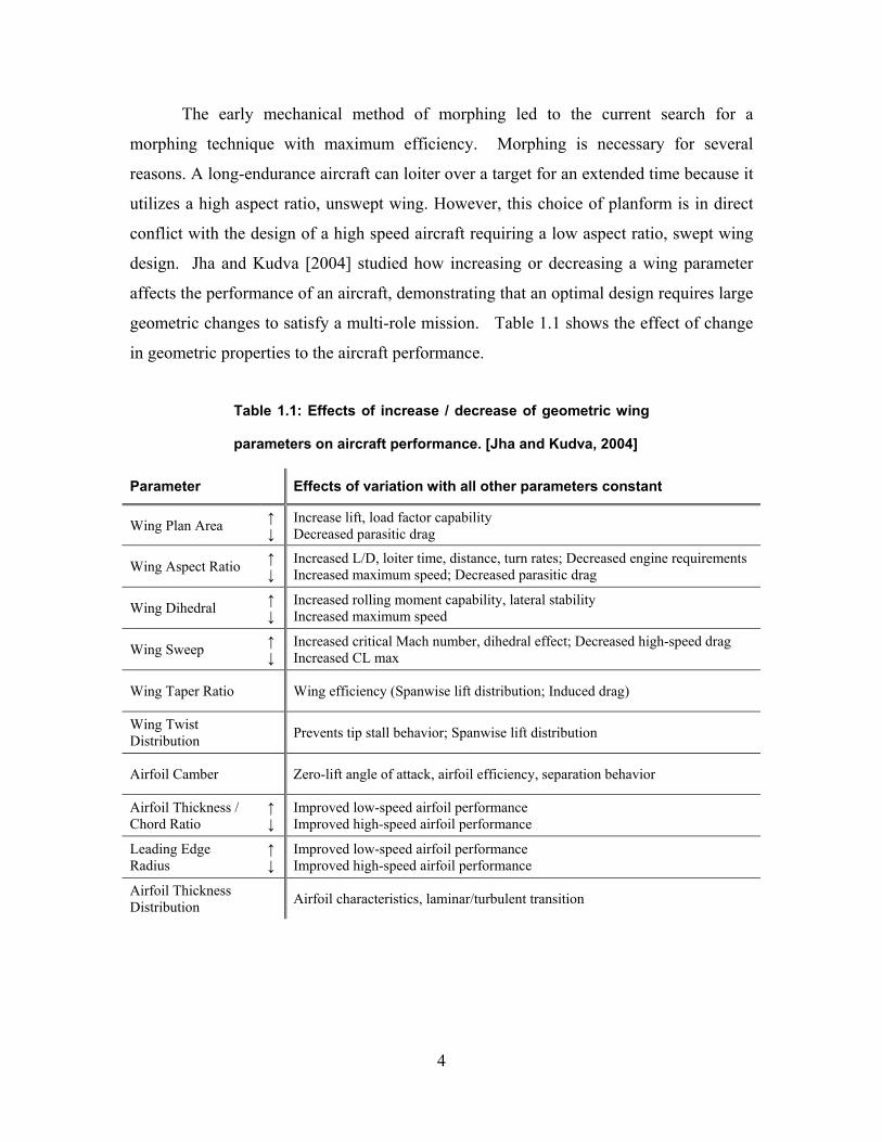
design. Jha and Kudva [2004] studied how increasing or decreasing a wing parameter

affects the performance of an aircraft, demonstrating that an optimal design requires large

geometric changes to satisfy a multi-role mission. Table 1.1 shows the effect of change

in geometric properties to the aircraft performance.

Table 1.1: Effects of increase / decrease of geometric wing

parameters on aircraft performance. [Jha and Kudva, 2004]

Parameter Effects of variation with all other parameters constant

Wing Plan Area ↑ ↓

Increase lift, load factor capability Decreased parasitic drag

Wing Aspect Ratio ↑ ↓

Increased L/D, loiter time, distance, turn rates; Decreased engine requirements Increased maximum speed; Decreased parasitic drag

Wing Dihedral ↑ ↓

Increased rolling moment capability, lateral stability Increased maximum speed

Wing Sweep ↑ ↓

Increased critical Mach number, dihedral effect; Decreased high-speed drag Increased CL max

Wing Taper Ratio Wing efficiency (Spanwise lift distribution; Induced drag)

Wing Twist Distribution Prevents tip stall behavior; Spanwise lift distribution

Airfoil Camber Zero-lift angle of attack, airfoil efficiency, separation behavior

Airfoil Thickness / Chord Ratio

↑ ↓

Improved low-speed airfoil performance Improved high-speed airfoil performance

Leading Edge Radius

↑ ↓

Improved low-speed airfoil performance Improved high-speed airfoil performance

Airfoil Thickness Distribution Airfoil characteristics, laminar/turbulent transition

4

While efficient low-speed flight requires a high aspect ratio and low sweep angle,

high-speed flight requires exactly the opposite. In order to have the same aircraft fly

diversified missions, it should be capable of making large geometric changes in an

efficient manner. Jha and Kudva [2004] reviewed several morphing wing concepts that

have been utilized. Examples will be briefly discussed below.

Camber control of wings using control surfaces has been extensively utilized in

the industry as a morphing concept. Most of these designs use discrete and rotating

leading and trailing edge controls. Trailing edge control is the more popular of the two.

The F-16 Fighting Falcon uses leading edge flaps to change the camber of the wings. In

2002, the Active Aeroelastic Wing program of NASA demonstrated twisting of wings for

primarily roll control at transonic and supersonic speeds for an F/A-18 Hornet. Twist

was achieved by creating aerodynamic moments on the wings by leading-edge flap and

aileron deflection.

The NASA-Ames Mission Adaptive Wing Research program focused on

producing smooth camber change by using a flexible internal mechanism to flex the outer

skin. Drag was reduced by around 7 percent at the wing design cruise point, and by 20

percent at an off-design condition.

Smooth cambering was applied in a Northrop Grumman UCAV test model. The

unmanned aircraft demonstrated high actuation rate (80deg/s), large deflection (20°),

hinge-less, smoothly contoured control surfaces with chord-wise and span-wise shape

variability. Piezoelectric motors were used as actuators [Bartley-Cho et al., 2002].

Continuous morphing concepts have also been utilized in smaller air vehicles.

Kim and Han [2006] designed and fabricated a smart flapping wing by using a

graphite/epoxy composite material and an MFC actuator. This study was aimed to mimic

the flapping motion of birds. Wind tunnel tests were performed to measure the

aerodynamic characteristic and performance of the surface actuators. A test stand was

also designed to measure the lift and thrust generated by the flapping device. The tests

were done on the Cybrid-P2 commercial ornithopter with and without the MFC actuator.

A twenty percent increase in lift was achieved by changing the camber of the wing at

different stages of flapping motion.

5

1.2.3 Smart Materials

The field of smart materials has advanced rapidly in the last 15 years due to an

increasing awareness of material capabilities, the development of new materials and

transducer designs, and increasingly stringent design and control specifications in

aerospace, aeronautic, industrial, automotive, biomedical, and nano-systems [Smith,

2005].

A piezoceramic material is a type of “smart material.” The history of

piezoelectricity dates to 1880 when Pierre and Jacques Curie discovered the effect in

several substances. The term piezoelectricity is used for certain materials and substances

that generate charge (or voltage) when pressure is applied to them [Inman and Cudney,

2000]. These materials are also capable of changing their shape when they are exposed

to an electric field. In short, piezoelectricity could be considered the coupling between

electrical and mechanical systems. The direct effect is the charge generated due to

pressure. The converse effect is the mechanical response of the material to the electrical

field.

Applications of piezoelectric materials are very broad. Among the other types of

active materials, piezoceramics exhibit several notable characteristics which render them

particularly useful in the area of structural control and sensing. Although the electrically

induced strains are relatively small (around 0.1%), the force outputs can be very large,

resulting in high energy density. Response times are also very short which allows for

high frequency applications. Piezoelectric materials exhibit high-sensitivity to

mechanical deformation which allows them to be used as sensors [Lloyd, 2004].

Selected electrical and mechanical properties of common piezoceramics can be seen in

Table 1.2. Uses for PZT-5A include accelerometers, hydrophones, low power structural

control, and stable sensors. PZT-5H is used in areas requiring sensitive receivers, fine

motion control, and low power structural control. The single crystal piezoceramic,

PMN-PT, is best suited to low induced-stress, high strain, and deflection applications

[Wilkie, 2006]. Two common types of piezoelectric materials are monolithic

piezoceramic plates and piezoelectric fiber composites.

6

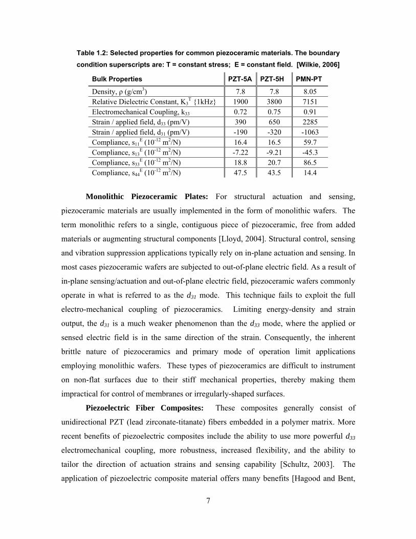
Table 1.2: Selected properties for common piezoceramic materials. The boundary condition superscripts are: T = constant stress; E = constant field. [Wilkie, 2006]

Bulk Properties PZT-5A PZT-5H PMN-PT

Density, ρ (g/cm3) 7.8 7.8 8.05 Relative Dielectric Constant, K3

T 1kHz 1900 3800 7151 Electromechanical Coupling, k33 0.72 0.75 0.91 Strain / applied field, d33 (pm/V) 390 650 2285 Strain / applied field, d31 (pm/V) -190 -320 -1063 Compliance, s11

E (10-12 m2/N) 16.4 16.5 59.7 Compliance, s13

E (10-12 m2/N) -7.22 -9.21 -45.3 Compliance, s33

E (10-12 m2/N) 18.8 20.7 86.5 Compliance, s44

E (10-12 m2/N) 47.5 43.5 14.4

Monolithic Piezoceramic Plates: For structural actuation and sensing,

piezoceramic materials are usually implemented in the form of monolithic wafers. The

term monolithic refers to a single, contiguous piece of piezoceramic, free from added

materials or augmenting structural components [Lloyd, 2004]. Structural control, sensing

and vibration suppression applications typically rely on in-plane actuation and sensing. In

most cases piezoceramic wafers are subjected to out-of-plane electric field. As a result of

in-plane sensing/actuation and out-of-plane electric field, piezoceramic wafers commonly

operate in what is referred to as the d31 mode. This technique fails to exploit the full

electro-mechanical coupling of piezoceramics. Limiting energy-density and strain

output, the d31 is a much weaker phenomenon than the d33 mode, where the applied or

sensed electric field is in the same direction of the strain. Consequently, the inherent

brittle nature of piezoceramics and primary mode of operation limit applications

employing monolithic wafers. These types of piezoceramics are difficult to instrument

on non-flat surfaces due to their stiff mechanical properties, thereby making them

impractical for control of membranes or irregularly-shaped surfaces.

Piezoelectric Fiber Composites: These composites generally consist of

unidirectional PZT (lead zirconate-titanate) fibers embedded in a polymer matrix. More

recent benefits of piezoelectric composites include the ability to use more powerful d33

electromechanical coupling, more robustness, increased flexibility, and the ability to

tailor the direction of actuation strains and sensing capability [Schultz, 2003]. The

application of piezoelectric composite material offers many benefits [Hagood and Bent,

7

1993]. Typically, crystalline materials have much higher strengths in fibrous form,

where the decreased volume fraction of flaws leads to an increase specific strength. Since

they will be encased in a polymer and laminated with other flexible layers, the fibers can

be thinner, thus less stiff in bending than a monolithic layer.

1.2.4 The Macro Fiber Composite

The MFC was developed at NASA Langley Research Center [Wilkie et al., 2000].

The MFC is a layered, planar actuation device that employs rectangular cross-section,

unidirectional piezoceramic fibers (PZT 5A) embedded in a thermosetting polymer

matrix. This active, fiber reinforced layer is then sandwiched between copper-clad

Kapton film layers that have an interdigitated electrode pattern. Figure 1.1 shows an

exploded view of the MFC layers, where the PZT fibers are aligned in the 3-direction and

the copper electrode fingers are parallel to the 1-direction, according to standard

piezoelectric notation [Williams, 2004].

Figure 1.1: The Macro Fiber Composite actuator. Left: A demonstration of the flexibility of the MFC. Right: Layers of the actuator.

A comprehensive manufacturing manual for MFC can be found in High and

Wilkie [2003]. The in-plane poling and subsequent voltage actuation allows the MFC to

utilize the d33 piezoelectric effect, which is much stronger than the d31 effect used by

traditional PZT actuators with through-the-thickness poling [Hagood et al., 1993]. MFC

has a uniform geometry, including PZT fiber and electrode spacing and continuity, as

well as the absence of air voids or particulate inclusions. The use of rectangular fibers

8

also promotes improved contact between the piezoceramic and the adjacent electrode

finger, thus ensuring more efficient transfer of electric field into the fibers.

There has been extensive analytical and experimental research focused on

utilizing MFC as an actuator (or sensor) for structural control. Williams [2004] provides

a detailed nonlinear characterization of the mechanical and piezoelectric behavior of the

MFC actuator. A classical lamination model was developed to predict MFC’s short

circuit linear-elastic properties. Piezoelectric characterization is achieved using a non-

linear actuation model whose parameters are experimentally determined. Common linear

piezoelectric strain coefficients are presented as a function of electric field and applied

stress.

MFC Applications: Moses et al. [2001] used both Active Fiber Composite

(AFC, an earlier version of MFC) and MFC to actively reduce vibration levels in the tail

fins of a wind-tunnel model of a fighter jet subjected to buffet loads. The model was

tested at a Mach Number of 0.105 and a 25 degree angle of attack. One fin had five

MFCs, while the other had five AFCs. Using a maximum closed-loop control signal input

of 1000 V to the actuators, the fin-tip peak acceleration was reduced by about 70% with

the MFCs and about 85% with the AFCs at frequencies near the first bending mode.

Torsional peak vibration levels were reduced 30% and 40% by delivering a closed-loop

control signal to the MFCs and AFCs respectively.

Sodano, Park, and Inman [2003] experimentally investigated the suitability of

using the MFC for structural vibration applications. Ground testing and active vibration

control of an inflated Kapton torus was performed using an MFC. By measuring changes

in impedance, the MFC was able to accurately detect damage in a lap joint whose bolt

preload was reduced, and in a cantilevered beam whose clamped end was loosened. In

addition, self-sensing technology was used with the MFC to reduce the vibration levels of

a cantilevered aluminum beam.

Ruggerio et al. [2002] used several MFCs as both actuators and sensors to

measure the dynamic behavior of the same inflated Kapton torus and to control its

vibration. The flexibility of MFC made attachment convenient to the curved surface. The

MFC was found to outperform other actuators and to have sensitivity comparable to other

monolithic piezoelectric sensors.

9

Schultz [2003] used the flexibility and high force output of the MFC to snap-

through an unsymmetric composite laminate from one stable configuration to another.

Using the MFC with such anisotropic structures could open the door to large-deflection

shape control including applications in morphing wing technology.

1.3 Objectives

Fabricating and successfully flying an MAV that uses MFCs for control is the

main objective for this research. Review of literature in the field of smart materials,

adaptive structures, and aerospace did not reveal a fully operational MAV which flies

using active materials as aerodynamic control surfaces. Hence, the research presented

herein is considered unique.

It must be noted that, in some cases, MAVs are defined as unmanned air vehicles

which weigh 50 grams or less and have a wing span less than 0.15 meters. The aircraft

presented in this work weighs 815 grams and has a 0.76 meter wingspan. In this thesis,

the aircraft will be referred to as an MAV since the main goal of continuing research is to

study the low Reynolds Number effects in small unmanned air vehicles.

From a broader perspective, the study aims to understand the behavior of

morphing wing micro air vehicles under low speed, quasi steady air flow. The aircraft

designed and fabricated will serve as a test bed for future research to improve flight

characteristics of small unmanned air vehicles.

1.4 Outline of the Thesis

Chapter 2 discusses the initial modeling and experimentation conducted to

understand the behavior of MFC actuated structures. Mathematical modeling is done

using the Rayleigh-Ritz method. Predictions of the displacement fields are plotted.

Several specimens are tested and compared to the model.

Chapter 3 presents the comparison of a variable camber airfoil to a conventional

airfoil. The lift and drag forces generated by the two airfoils are measured using a

mechanical balance in a wind tunnel. Performance of the airfoils are discussed.

10

Chapter 4 presents the experimental aircraft design. Design requirements are

discussed and the components of the MAV are presented. The chapter concludes with a

summary of specifications of the fabricated aircraft.

Chapter 5 discusses the experiments conducted on the aircraft to quantify its

performance. Wind tunnel tests are conducted at 10.3 m/s for different angle of attack

settings. Lift, drag and roll characteristics are presented. Also in this chapter, flight tests

are described and an analysis of the flight video is shown.

Chapter 6 provides a summary of the results from the research. The conference

publications stemming from the research are listed. A discussion of recommendations for

improvements and future work is presented.

In addition to the chapters outlined above, the thesis includes a set of appendices

that present detailed derivations or additional information related to the chapters.

Appendix A presents the detailed derivation of orthotropic properties of the MFC

actuator using the classical lamination theory. The results calculated from the theory are

used to aid the Rayleigh-Ritz method presented in Chapter 2. Appendix B presents the

fabrication and the operation of the mechanical balance, which is employed in the wind

tunnel experiment in Chapter 3. Appendix C shows the calculations for the flow speed

adjustment necessary for the wind tunnel experiment presented in Chapter 3. Appendix

D presents the mold design for the wings and an experimental analysis of the electronic

circuit employed in the aircraft. Appendix E demonstrates the additional test results from

the wind tunnel experiments conducted on the aircraft. The results of these wind tunnel

experiments are summarized in Chapter 5.

11

Chapter 2: Modeling and Experimentation of MFC

Actuated Laminates

In order to predict the displacement generated by an MFC actuator on the

composite material, the Rayleigh-Ritz technique was utilized. This approximation

technique was used by Schultz [2003, 2004] to predict the snap-through behavior of

unsymmetric crossply laminates. The modeling work in this chapter is based on

Schultz’s studies. The technique relies on a good approximation of displacement fields

which has been studied by Hyer [1981]. First, four-term displacement fields were

assumed for defection in x, y and z coordinates. Strain energy was calculated in terms of

the displacement fields for the actuator and the “host” material that was being actuated.

Total potential energy of the system was calculated by adding the strain energy of the

actuator and host. The unknown constants were then solved by searching for the

stationary values of the total potential energy of the combined laminate.

An extension of classical lamination theory (CLT) was used to predict to

engineering properties of the MFC actuator. These values define the “stiffness” of the

MFC. The predicted values were compared to the ones from the manufacturer. The

results from CLT provided good insight to the mechanics of the MFC actuator.

This chapter will first present the classical lamination theory and predictions of

the material properties for the MFC and the host laminates. Next, the Rayleigh-Ritz

method will be discussed. Finally, experiments will be presented and compared to the

Rayleigh-Ritz model.

2.1 Classical Lamination Theory

MFC is composed of both isotropic and orthotropic layers. It is most adequately

described as a symmetric, hybrid, cross-ply laminate, or [IsoKapton / IsoAcrylic / 90°Copper /

0° PZT ]s. The overall mechanical behavior of this orthotropic laminate is described by

12

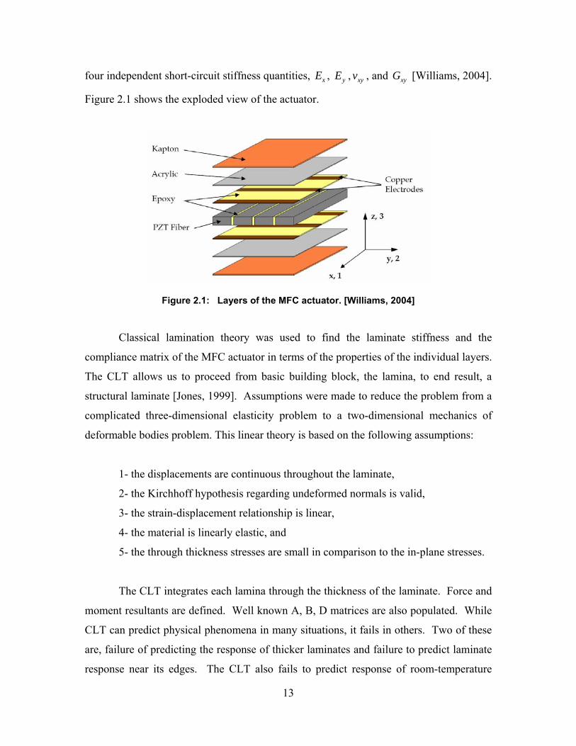
four independent short-circuit stiffness quantities, , xE yE , , and [Williams, 2004].

Figure 2.1 shows the exploded view of the actuator.

xyv xyG

Figure 2.1: Layers of the MFC actuator. [Williams, 2004]

Classical lamination theory was used to find the laminate stiffness and the

compliance matrix of the MFC actuator in terms of the properties of the individual layers.

The CLT allows us to proceed from basic building block, the lamina, to end result, a

structural laminate [Jones, 1999]. Assumptions were made to reduce the problem from a

complicated three-dimensional elasticity problem to a two-dimensional mechanics of

deformable bodies problem. This linear theory is based on the following assumptions:

1- the displacements are continuous throughout the laminate,

2- the Kirchhoff hypothesis regarding undeformed normals is valid,

3- the strain-displacement relationship is linear,

4- the material is linearly elastic, and

5- the through thickness stresses are small in comparison to the in-plane stresses.

The CLT integrates each lamina through the thickness of the laminate. Force and

moment resultants are defined. Well known A, B, D matrices are also populated. While

CLT can predict physical phenomena in many situations, it fails in others. Two of these

are, failure of predicting the response of thicker laminates and failure to predict laminate

response near its edges. The CLT also fails to predict response of room-temperature

13

shapes of thin unsymmetric laminates. Hyer [1981] has showed room-temperature

shapes of some thin unsymmetric laminates are closely approximated by right circular

cylinders. In addition, some unsymmetric laminates have two cylindrical shapes. To

predict the shapes accurately, it is necessary to include nonlinearities along into the CLT.

The CLT was applied to MFC and the stiffness values were calculated. Appendix

A shows the complete derivation. Engineering properties were calculated to be:

. These predictions

were in good agreement with the values from the manufacturer.

30.7 GPa, 14.4 GPa, 0.267, and 4.10 GPaMFC MFC MFC MFCx y xy xyE E v G= = = =

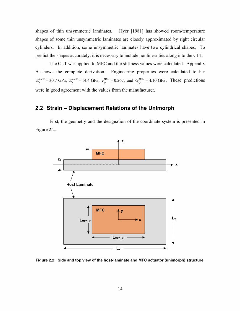
2.2 Strain – Displacement Relations of the Unimorph

First, the geometry and the designation of the coordinate system is presented in

Figure 2.2.

z

Figure 2.2: Side and top view of the host-laminate and MFC actuator (unimorph) structure.

Host Laminate

MFC

x

y

LY

LX

LMFC, Y

LMFC, X

MFCz2

z3

x z0

14

The non-linear strain-displacement relationship for small strains and rotations in

the laminates are given by Equation 2.1.

2

2

12

12

x

y

xy

u wx x

v wy y

u v w wy x x y

ε

ε

γ

⎛ ⎞∂ ∂= + ⎜ ⎟∂ ∂⎝ ⎠

⎛ ⎞∂ ∂= + ⎜ ⎟∂ ∂⎝ ⎠

⎛ ⎞⎛ ⎞∂ ∂ ∂ ∂= + + ⎜ ⎟⎜ ⎟∂ ∂ ∂ ∂⎝ ⎠⎝ ⎠

(2.1)

where are the displacements of the structure in the , , andu v w , , andx y z directions

respectively. These strain-displacement relationships will be used for both host laminate

and the MFC actuator. The midplane curvatures in terms of the displacements are:

2

2

2

2

2

2

x

y

xy

wxwy

wx y

κ

κ

κ

∂= −

∂∂

= −∂

∂= −

∂ ∂

(2.2)

According to the Kirchhoff hypotheses, the strains at any z location in terms of

the midplane strains and curvatures are:

x x x

y y y

xy xy xy

z

z

z

ε ε κ

ε ε κ

γ γ κ

= +

= +

= +

(2.3)

Four-term displacement terms, given in Equation 2.4, were used for the three

components of the displacement of the midplane geometry.

15

2 3 21 1 2

3

2 3 22 1 2

4

2 21 2

( , )6 4

( , )6 4

1( , ) ( )2

c x c c xyu x y c x

c y c c x yv x y c y

w x y c x c y

= − −

= − −

= +

(2.4)

The midplane strains and curvatures in terms of unknown coefficients , , ,

are given by Equation 2.5.

1c 2c 3c

4c

21 2

3

21 2

4

4

40

x

y

xy

c c yc

c c xc

ε

ε

γ

= −

= −

=

1

2

0

x

y

xy

c

c

κ

κ

κ

= −

= −

=

(2.5)

2.3 Potential Energy Calculations

Potential energy of the actuator / host structure is calculated in several steps.

First, the host laminate is evaluated. Next, MFC actuator with no applied voltage is

evaluated. Finally, the MFC actuator with applied voltage is studied. Total potential

energy of the unimorph structure with applied voltage is found by adding the strain

energy contribution from the host laminate and the strain energy contribution from the

MFC actuator (with applied voltage). Modeling process is described in the following

sections.

2.3.1 Host Laminate Potential Energy

The total potential energy of the host laminate is calculated by:

2

0

( / 2)( / 2)

( / 2) ( / 2)

1 [2

yx

x y

LL z

HOST x x y y xy xyL L z

U dσ ε σ ε σ γ− −

= + +∫ ∫ ∫ ] x dy dz (2.6)

where σ s are the stresses, ε s and the xyγ are the strains, the and are the side

lengths of the laminate, and the

xL yL

0z and 2z are the location of the bottom and the top layer

16

of the host laminate. Since the host laminates in the tests are the same size as the MFC

patch, we can designate and ,x MFCL L= x y,y MFCL L= where MFCL s are the side lengths of

the MFC 4010 actuator. The stresses are given by:

11 12 16

12 22 26

16 26 66

x x y x

y x y

xy x y xy

Q Q Q

Q Q Q

Q Q Q

y

xy

σ ε ε γ

σ ε ε γ

σ ε ε

= + +

= + +

= + + γ

or x x

y HOST y

xy xyHOST HOST

Qσ εσσ γ

⎧ ⎫ ⎧ ⎫⎪ ⎪ ⎪ ⎪=⎨ ⎬ ⎨ ⎬⎪ ⎪ ⎪ ⎪⎩ ⎭ ⎩ ⎭

ε (2.7)

where Q s are the transformed reduced stiffness of the host laminate that is being

considered. HOSTQ is the transformed reduced stiffness matrix of the host laminate. The

16Q and 26Q are zero for all laminates considered in the experiments.

Substituting the stress and strain equations in the total potential equation and

carrying out the triple integration, total energy reduces to an algebraic equation in terms

of the unknown constants , , , and . 1c 2c 3c 4c

2.3.2 Actuator Potential Energy without Applied Voltage

The total potential energy of the actuator with no applied voltage is calculated

similar to the host material. Strain energy is given by Equation 2.8.

,, 3

, , 2

( / 2)( / 2)

, , , ,( / 2) ( / 2)

, ,

1 [2

]

MFC yMFC x

MFC x MFC y

LL z

NA MFC x MFC x MFC y MFC yL L z

MFC xy MFC xy

U

dx dy dz

σ ε σ ε

σ γ− −

= +

+

∫ ∫ ∫ (2.8)

where MFCσ s are the stresses and the MFCε s and ,MFC xyγ are the strains in the MFC

actuator. As mentioned before MFCL s are the side lengths of the MFC actuator. The

dimension along thickness of the actuator is designated by 2z and 3z , bottom and top

surface of the MFC respectively.

The stress developed in the actuator is due to the MFC being bent to the same

curvature of the host laminate. Stress in the MFC actuator in matrix form is:

17

x x

y MFC y

xy xyMFC MFC

Qσ εσσ γ

⎧ ⎫ ⎧ ⎫⎪ ⎪ ⎪ ⎪=⎨ ⎬ ⎨ ⎬⎪ ⎪ ⎪ ⎪⎩ ⎭ ⎩ ⎭

ε (2.9)

where MFCQ is the transformed reduced stiffness matrix of the MFC. Curvatures of the

midsurface of the laminate and the midsurface of the actuator are assumed to be the same

rather than the curvatures of the contacting surfaces. The strains in the actuator are

approximated by:

3 0

2

x x

y

xy xyMFC

z zz y

ε κε κγ κ

⎧ ⎫⎧ ⎫⎛ − ⎞⎪ ⎪⎪ ⎪ ⎛ ⎞= −⎨ ⎬ ⎨ ⎬⎜ ⎟⎜ ⎟

⎝ ⎠⎝ ⎠⎪ ⎪ ⎪ ⎪⎩ ⎭ ⎩ ⎭

(2.10)

where since and 0xyγ = 0xyκ = xκ and yκ are the unknown midsurface curvatures for

both the actuator and the host material. Four-term displacements fields used before are

assumed and substitutions are carried out similar to host material. Potential energy can

be written in terms of the unknown constants , , , and . 1c 2c 3c 4c

2.3.3 Total Potential Energy of the Actuator - Host (0 Volts)

Total strain energy is sum of the potential energy of the host material and the

actuator in terms of the unknown constants.

(2.11) 1 1 2 3 4 1 2 3 4( , , , ) ( , , , )HOST NAU U c c c c U c c c c= +

The constants are found by minimizing the total potential energy by setting the

first variation of the total energy to zero.

1 0 1, 2,3, 4i

U ic

∂= =

∂ (2.12)

This system of nonlinear algebraic equations was solved in MATLAB. When flat

laminates were modeled (no curvature), the unknown coefficients, - , were equal to 1c 4c

18

zero. This was expected because no external stress is applied to the unimorph or no

strain is induced due to curvature.

2.3.4 Actuator Potential Energy with Applied Voltage

The previous MFC actuator model had to be adjusted to include piezoelectric

effect. The potential energy of the actuator includes strains due to bending and due to

applied voltage. The potential energy is written as:

,, 3

, , 2

( / 2)( / 2)

, , , ,( / 2) ( / 2)

, , , , , ,

1 [( )2

( ) ( ) ]

MFC yMFC x

MFC x MFC y

LL z

MFC actuated MFC x Piezo x MFC xL L z

MFC y Piezo y MFC y MFC xy Piezo xy MFC xy

U

dx dy dz

σ σ ε

σ σ ε σ σ γ

− −

= −

+ − + −

∫ ∫ ∫ (2.13)

where MFCε s and ,MFC xyγ are the strains in the MFC actuator with voltage applied. These

strain terms are more complicated than non-actuated MFC and will be discussed later.

The MFCσ s are the stresses in the actuator and are given by:

x x

y MFC y y

xy xy xy

x

MFC MFC Piezo

Qσ εσ εσ γ σ

⎧ ⎫ ⎧ ⎫ ⎧ ⎫⎪ ⎪ ⎪ ⎪ ⎪ ⎪= −⎨ ⎬ ⎨ ⎬ ⎨ ⎬⎪ ⎪ ⎪ ⎪ ⎪ ⎪⎩ ⎭ ⎩ ⎭ ⎩ ⎭

σσ (2.14)

The induced stresses due to actuation voltage are given by:

x x

y MFC y

xy xyPiezo Piezo

Qσ εσσ γ

⎧ ⎫ ⎧ ⎫⎪ ⎪ ⎪ ⎪=⎨ ⎬ ⎨ ⎬⎪ ⎪ ⎪ ⎪⎩ ⎭ ⎩ ⎭

ε (2.15)

where the Piezoε s and ,Piezo xyγ are the piezoelectrically-induced strains. The piezoelectric

strains due to applied voltage are given by Equation 2.16.

19

11

121 0

x

y

xy Piezo

dV dx

εεγ

⎧ ⎫ ⎧ ⎫∆⎪ ⎪ ⎪ ⎪=⎨ ⎬ ⎨∆ ⎬

⎪ ⎪ ⎪⎩ ⎭⎩ ⎭

⎪ (2.16)

where s are the effective piezoelectric coefficients, d V∆ is the applied voltage to the

MFC actuator, and the is the distance between the interdigitated electrodes on the

MFC. The strains in the actuator are:

1x∆

x x x

y y y

xy xy xyMFC NA Shift

ε ε εε ε εγ γ γ

⎧ ⎫ ⎧ ⎫ ⎧ ⎫⎪ ⎪ ⎪ ⎪ ⎪ ⎪= −⎨ ⎬ ⎨ ⎬ ⎨ ⎬⎪ ⎪ ⎪ ⎪ ⎪ ⎪⎩ ⎭ ⎩ ⎭ ⎩ ⎭

(2.17)

where ε s and the xyγ are the Kirchhoff-like strains that are zero at the laminate

midsurface and vary linearly with thickness. These strains are the same as in the non-

actuated MFC and are given by:

3 0

2

x x

y

xy xyNA

z zz y

ε κε κγ κ

⎧ ⎫⎧ ⎫⎛ − ⎞⎪ ⎪⎪ ⎪ ⎛ ⎞= −⎨ ⎬ ⎨ ⎬⎜ ⎟⎜ ⎟

⎝ ⎠⎝ ⎠⎪ ⎪ ⎪ ⎪⎩ ⎭ ⎩ ⎭

(2.18)

The shift strains, Shiftε s and the ,Shift xyγ , take into account of the discontinuous

through thickness strains due to room temperature bonding of the actuator to the host

laminate. These shift strains are:

3 0

2

x x x

y y y

xy xy xyShift Initial Initial

z zε ε κε ε κγ γ κ

⎧ ⎫ ⎧ ⎫ ⎧ ⎫−⎪ ⎪ ⎪ ⎪ ⎪ ⎪⎛ ⎞= +⎨ ⎬ ⎨ ⎬ ⎨ ⎬⎜ ⎟

⎝ ⎠⎪ ⎪ ⎪ ⎪ ⎪ ⎪⎩ ⎭ ⎩ ⎭ ⎩ ⎭

(2.19)

where the s and the are the initial midsurface strains and s are the

initial midsurface curvatures. These initial strain and curvature values are calculated by

using from Equation 2.12. These constants are plugged into Equation 2.20 and

initial strains and curvatures are calculated.

Initialε ,Initial xyγ Initialκ

1c c− 4

20

21 2

, 3

21 2

, 4

,

4

40

x Initial

y Initial

xy Initial

c c yc

c c xc

ε

ε

γ

= −

= −

=

, 1

,

, 0

x Initial

y Initial

xy Initial

c

c

κ

κ

κ2

= −

= −

=

(2.20)

2.3.5 Total Potential Energy of the Actuator - Host with Applied

Voltage

Total strain energy is sum of the potential energy of the host material and the

actuator in terms of the unknown constants.

(2.21) 2 1 2 3 4 , 1 2 3 4( , , , ) ( , , , )HOST MFC actuatedU U c c c c U c c c c= +

The unknown constants are found by minimizing the total potential energy by

setting the first variation of the total energy to zero.

2 0 1, 2,3, 4i

U ic

∂= =

∂ (2.22)

This system of nonlinear algebraic equations was solved in MATLAB. The

stability of the solution is checked by examining positive definitiveness of the second

variation of the total potential energy.

2.4 Prediction of Displacement Fields

The parameters such as material constants and dimensions were entered in to the

model which was coded in MATLAB. Adjustments to the laminate thickness and

piezoelectric constants had to be made to get the accurate shapes. To make these

adjustments, a calibration experiment was performed with aluminum and stainless steel

host material in different thicknesses. The effective parameters were then used to predict

21

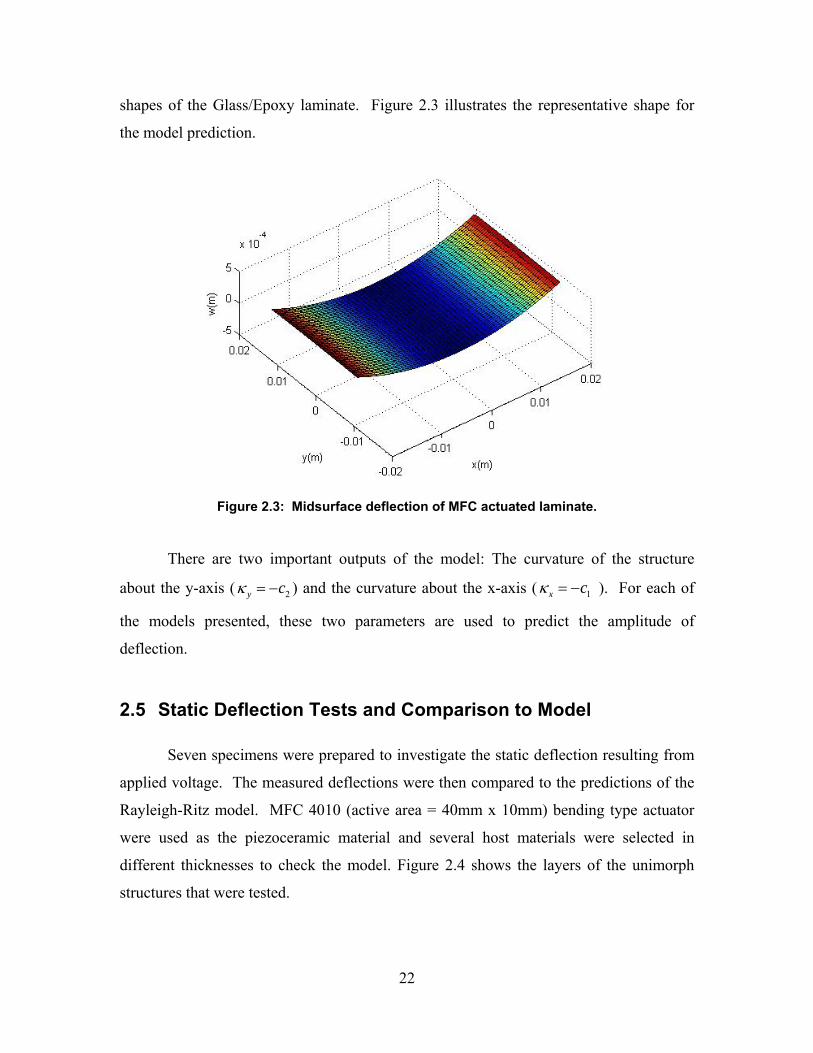
shapes of the Glass/Epoxy laminate. Figure 2.3 illustrates the representative shape for

the model prediction.

Figure 2.3: Midsurface deflection of MFC actuated laminate.

There are two important outputs of the model: The curvature of the structure

about the y-axis ( ) and the curvature about the x-axis (2y cκ = − 1x cκ = − ). For each of

the models presented, these two parameters are used to predict the amplitude of

deflection.

2.5 Static Deflection Tests and Comparison to Model

Seven specimens were prepared to investigate the static deflection resulting from

applied voltage. The measured deflections were then compared to the predictions of the

Rayleigh-Ritz model. MFC 4010 (active area = 40mm x 10mm) bending type actuator

were used as the piezoceramic material and several host materials were selected in

different thicknesses to check the model. Figure 2.4 shows the layers of the unimorph

structures that were tested.

22

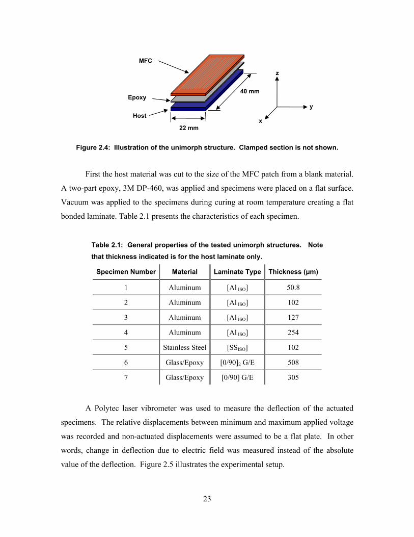
Figure 2.4: Illustration of the unimorph structure. Clamped section is not shown.

First the host material was cut to the size of the MFC patch from a blank material.

A two-part epoxy, 3M DP-460, was applied and specimens were placed on a flat surface.

Vacuum was applied to the specimens during curing at room temperature creating a flat

bonded laminate. Table 2.1 presents the characteristics of each specimen.

Table 2.1: General properties of the tested unimorph structures. Note that thickness indicated is for the host laminate only.

Specimen Number Material Laminate Type Thickness (µm)

1 Aluminum [Al ISO] 50.8

2 Aluminum [Al ISO] 102



5 Stainless Steel [SSISO] 102

6 Glass/Epoxy [0/90]2 G/E 508

7 Glass/Epoxy [0/90] G/E 305

A Polytec laser vibrometer was used to measure the deflection of the actuated

specimens. The relative displacements between minimum and maximum applied voltage

was recorded and non-actuated displacements were assumed to be a flat plate. In other

words, change in deflection due to electric field was measured instead of the absolute

value of the deflection. Figure 2.5 illustrates the experimental setup.

40 mm

Host

MFC

z

Epoxy

x

y

22 mm

23

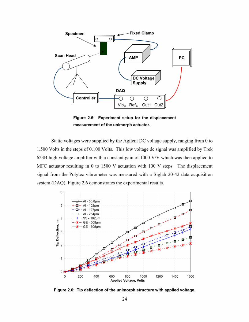
Fixed Clamp Specimen

Figure 2.5: Experiment setup for the displacement measurement of the unimorph actuator.

Static voltages were supplied by the Agilent DC voltage supply, ranging from 0 to

1.500 Volts in the steps of 0.100 Volts. This low voltage dc signal was amplified by Trek

623B high voltage amplifier with a constant gain of 1000 V/V which was then applied to

MFC actuator resulting in 0 to 1500 V actuation with 100 V steps. The displacement

signal from the Polytec vibrometer was measured with a Siglab 20-42 data acquisition

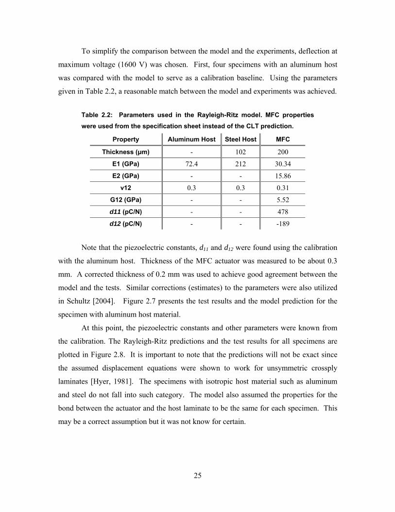
system (DAQ). Figure 2.6 demonstrates the experimental results.

0

1

2

3

4

5

6

0 200 400 600 800 1000 1200 1400 1600Applied Voltage, Volts

Tip

Def

lect

ion,

mm

Al - 50.8µmAl - 102µmAl - 127µmAl - 254µmSS - 102µmGE - 508µmGE - 305µm

Figure 2.6: Tip deflection of the unimorph structure with applied voltage.

Vibin Refin Out1 Out2

AMP Scan Head PC

DC Voltage Supply

DAQ

Controller

24

To simplify the comparison between the model and the experiments, deflection at

maximum voltage (1600 V) was chosen. First, four specimens with an aluminum host

was compared with the model to serve as a calibration baseline. Using the parameters

given in Table 2.2, a reasonable match between the model and experiments was achieved. Table 2.2: Parameters used in the Rayleigh-Ritz model. MFC properties were used from the specification sheet instead of the CLT prediction.

Property Aluminum Host Steel Host MFC

Thickness (µm) - 102 200

E1 (GPa) 72.4 212 30.34

E2 (GPa) - - 15.86

v12 0.3 0.3 0.31

G12 (GPa) - - 5.52

d11 (pC/N) - - 478

d12 (pC/N) - - -189

Note that the piezoelectric constants, d11 and d12 were found using the calibration

with the aluminum host. Thickness of the MFC actuator was measured to be about 0.3

mm. A corrected thickness of 0.2 mm was used to achieve good agreement between the

model and the tests. Similar corrections (estimates) to the parameters were also utilized

in Schultz [2004]. Figure 2.7 presents the test results and the model prediction for the

specimen with aluminum host material.

At this point, the piezoelectric constants and other parameters were known from

the calibration. The Rayleigh-Ritz predictions and the test results for all specimens are

plotted in Figure 2.8. It is important to note that the predictions will not be exact since

the assumed displacement equations were shown to work for unsymmetric crossply

laminates [Hyer, 1981]. The specimens with isotropic host material such as aluminum

and steel do not fall into such category. The model also assumed the properties for the

bond between the actuator and the host laminate to be the same for each specimen. This

may be a correct assumption but it was not know for certain.

25

Experiment

Model

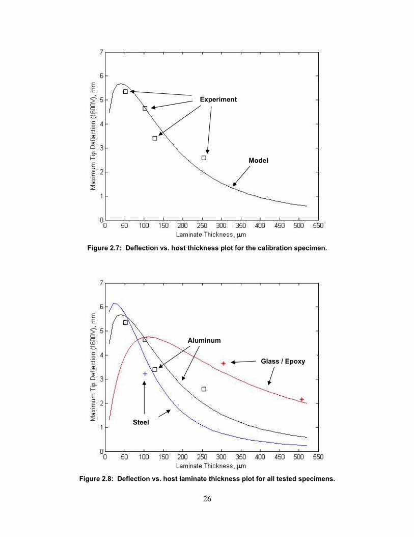
Figure 2.7: Deflection vs. host thickness plot for the calibration specimen.

Glass / Epoxy

Aluminum

Steel

Figure 2.8: Deflection vs. host laminate thickness plot for all tested specimens.

26

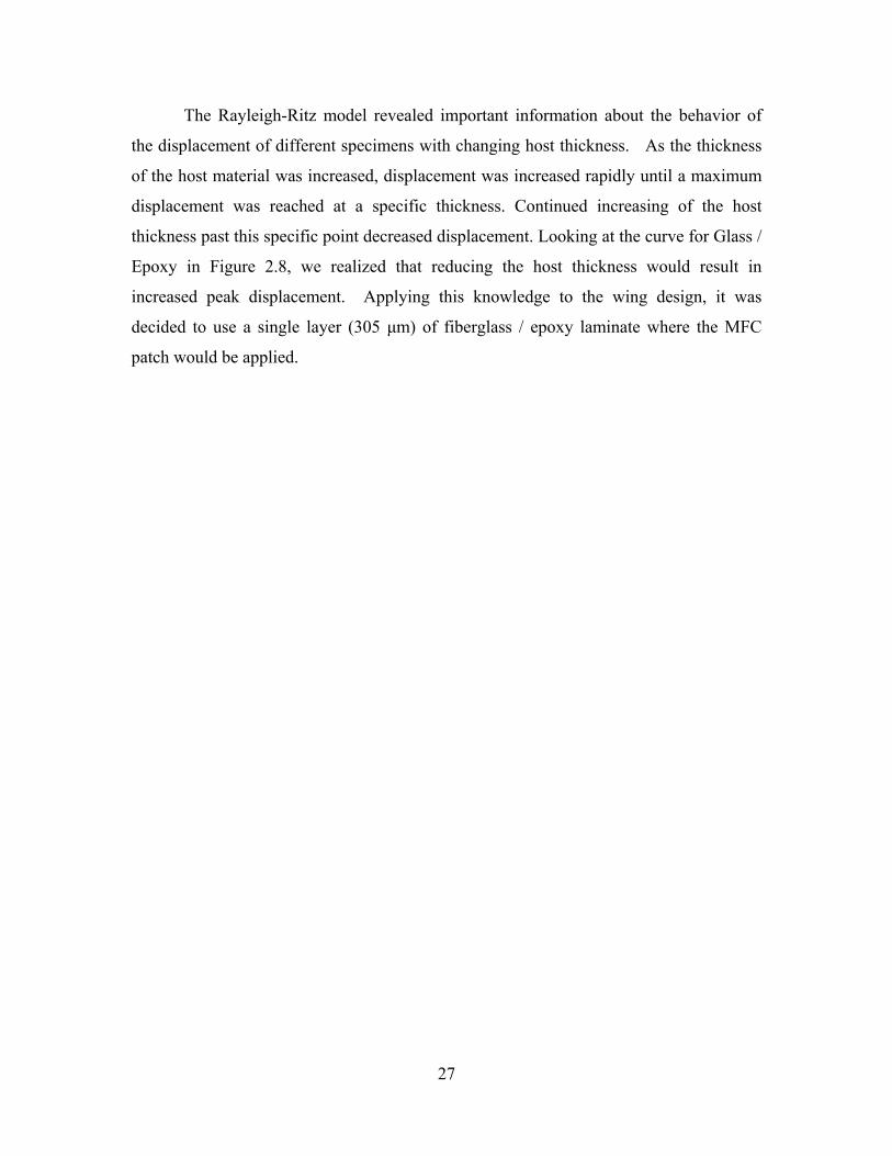
The Rayleigh-Ritz model revealed important information about the behavior of

the displacement of different specimens with changing host thickness. As the thickness

of the host material was increased, displacement was increased rapidly until a maximum

displacement was reached at a specific thickness. Continued increasing of the host

thickness past this specific point decreased displacement. Looking at the curve for Glass /

Epoxy in Figure 2.8, we realized that reducing the host thickness would result in

increased peak displacement. Applying this knowledge to the wing design, it was

decided to use a single layer (305 µm) of fiberglass / epoxy laminate where the MFC

patch would be applied.

27

Chapter 3: Wind Tunnel Experimentation on a

Morphing Airfoil

Wind tunnel tests were conducted to compare a variable camber airfoil (MFC

actuated) and a flapped (conventional) airfoil which were fabricated from a

fiberglass/epoxy composite material. The base shape for both airfoils was chosen to be a

thin circular arc with 1.8 percent camber. The circular arc wing was used because it has

been judged to be a superior low Reynolds Number airfoil by small-aircraft designers

[Hoffman, 1955]. The initial camber of the airfoil provides stiffness in the spanwise

direction to resist bending under aerodynamic loading. The test wing sections had a 108

mm chord and a 108 mm span. The composite material was laid up in a CNC (computer

numerical control) machined mold and vacuum bagged to cure at room temperature. The

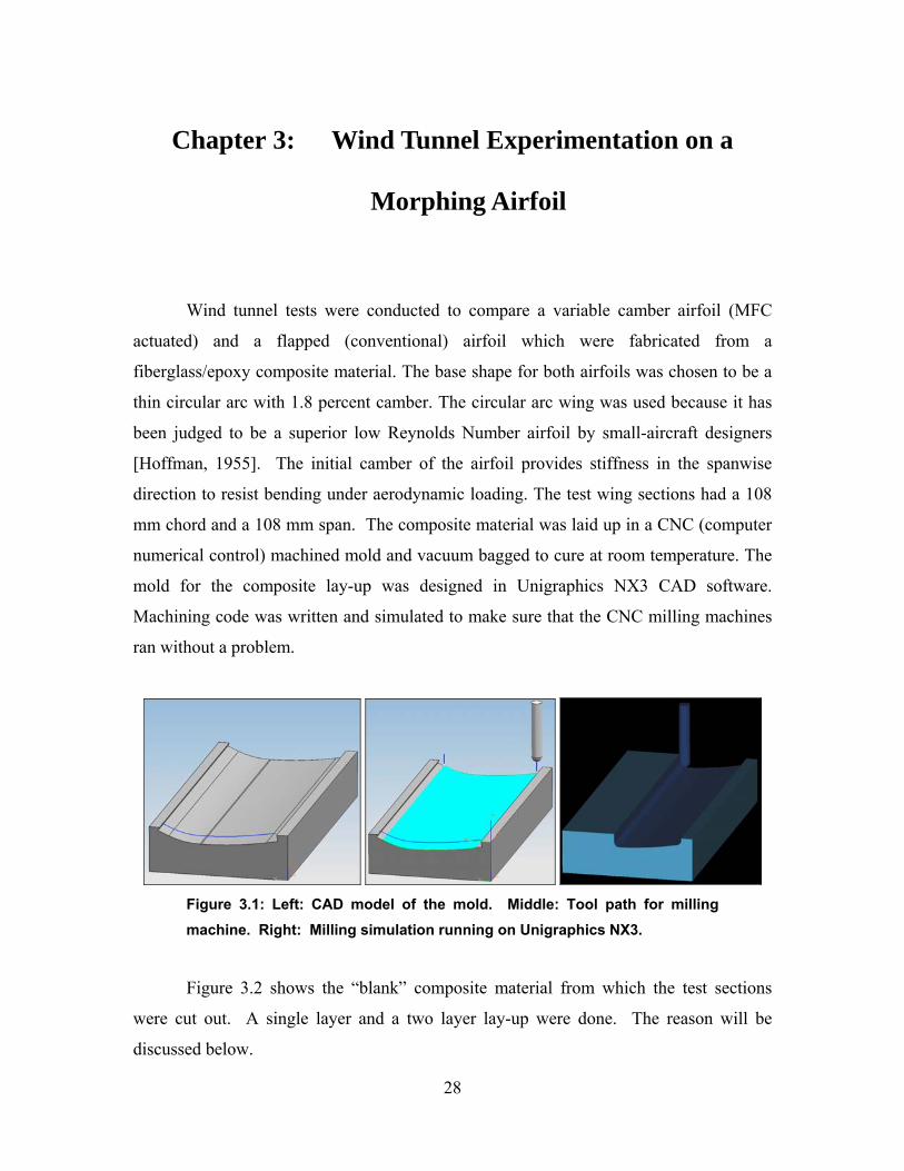
mold for the composite lay-up was designed in Unigraphics NX3 CAD software.

Machining code was written and simulated to make sure that the CNC milling machines

ran without a problem.

Figure 3.1: Left: CAD model of the mold. Middle: Tool path for milling machine. Right: Milling simulation running on Unigraphics NX3.

Figure 3.2 shows the “blank” composite material from which the test sections

were cut out. A single layer and a two layer lay-up were done. The reason will be

discussed below.

28

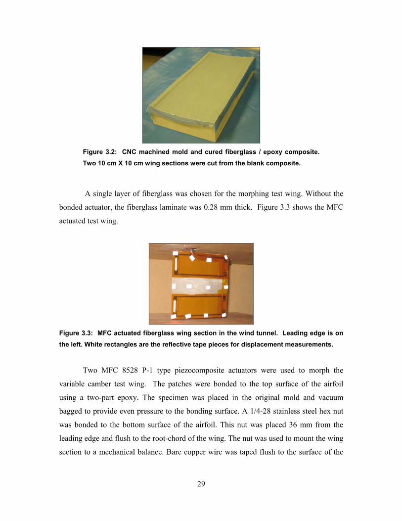
Figure 3.2: CNC machined mold and cured fiberglass / epoxy composite. Two 10 cm X 10 cm wing sections were cut from the blank composite.

A single layer of fiberglass was chosen for the morphing test wing. Without the

bonded actuator, the fiberglass laminate was 0.28 mm thick. Figure 3.3 shows the MFC

actuated test wing.

Figure 3.3: MFC actuated fiberglass wing section in the wind tunnel. Leading edge is on the left. White rectangles are the reflective tape pieces for displacement measurements.

Two MFC 8528 P-1 type piezocomposite actuators were used to morph the

variable camber test wing. The patches were bonded to the top surface of the airfoil

using a two-part epoxy. The specimen was placed in the original mold and vacuum

bagged to provide even pressure to the bonding surface. A 1/4-28 stainless steel hex nut

was bonded to the bottom surface of the airfoil. This nut was placed 36 mm from the

leading edge and flush to the root-chord of the wing. The nut was used to mount the wing

section to a mechanical balance. Bare copper wire was taped flush to the surface of the

29

wing with Kapton tape. The tape provided excellent electrical insulation considering high

voltages up to 1800 V.

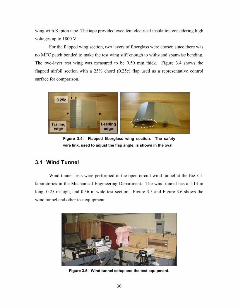
For the flapped wing section, two layers of fiberglass were chosen since there was

no MFC patch bonded to make the test wing stiff enough to withstand spanwise bending.

The two-layer test wing was measured to be 0.50 mm thick. Figure 3.4 shows the

flapped airfoil section with a 25% chord (0.25c) flap used as a representative control

surface for comparison.

Leading edge

Trailing edge

0.25c

Figure 3.4: Flapped fiberglass wing section. The safety wire link, used to adjust the flap angle, is shown in the oval.

3.1 Wind Tunnel

Wind tunnel tests were performed in the open circuit wind tunnel at the ExCCL

laboratories in the Mechanical Engineering Department. The wind tunnel has a 1.14 m

long, 0.25 m high, and 0.36 m wide test section. Figure 3.5 and Figure 3.6 shows the

wind tunnel and other test equipment.

Figure 3.5: Wind tunnel setup and the test equipment.

30

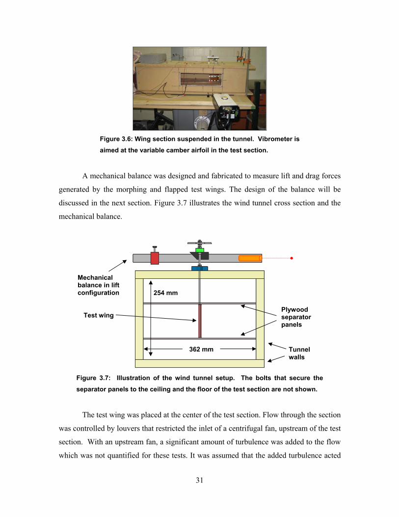
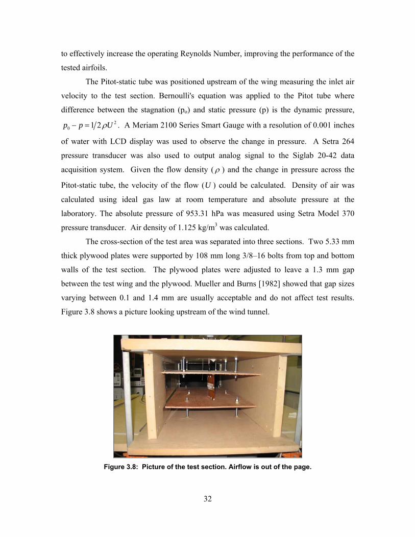
Figure 3.6: Wing section suspended in the tunnel. Vibrometer is aimed at the variable camber airfoil in the test section.

A mechanical balance was designed and fabricated to measure lift and drag forces

generated by the morphing and flapped test wings. The design of the balance will be

discussed in the next section. Figure 3.7 illustrates the wind tunnel cross section and the

mechanical balance.

362 mm

Plywood separator panels

Test wing

Mechanical balance in lift configuration 254 mm

Tunnel walls

Figure 3.7: Illustration of the wind tunnel setup. The bolts that secure the separator panels to the ceiling and the floor of the test section are not shown.

The test wing was placed at the center of the test section. Flow through the section

was controlled by louvers that restricted the inlet of a centrifugal fan, upstream of the test

section. With an upstream fan, a significant amount of turbulence was added to the flow

which was not quantified for these tests. It was assumed that the added turbulence acted

31

to effectively increase the operating Reynolds Number, improving the performance of the

tested airfoils.

The Pitot-static tube was positioned upstream of the wing measuring the inlet air

velocity to the test section. Bernoulli's equation was applied to the Pitot tube where

difference between the stagnation (po) and static pressure (p) is the dynamic pressure, 2

0 1 2p p Uρ− = . A Meriam 2100 Series Smart Gauge with a resolution of 0.001 inches

of water with LCD display was used to observe the change in pressure. A Setra 264

pressure transducer was also used to output analog signal to the Siglab 20-42 data

acquisition system. Given the flow density ( ρ ) and the change in pressure across the

Pitot-static tube, the velocity of the flow (U ) could be calculated. Density of air was

calculated using ideal gas law at room temperature and absolute pressure at the

laboratory. The absolute pressure of 953.31 hPa was measured using Setra Model 370

pressure transducer. Air density of 1.125 kg/m3 was calculated.

The cross-section of the test area was separated into three sections. Two 5.33 mm

thick plywood plates were supported by 108 mm long 3/8–16 bolts from top and bottom

walls of the test section. The plywood plates were adjusted to leave a 1.3 mm gap

between the test wing and the plywood. Mueller and Burns [1982] showed that gap sizes

varying between 0.1 and 1.4 mm are usually acceptable and do not affect test results.

Figure 3.8 shows a picture looking upstream of the wind tunnel.

Figure 3.8: Picture of the test section. Airflow is out of the page.

32

A cutout was made on the tunnel side wall and an acrylic sheet was bonded flush

with the inside surface of the tunnel to allow for displacement measurements with the

laser vibrometer.

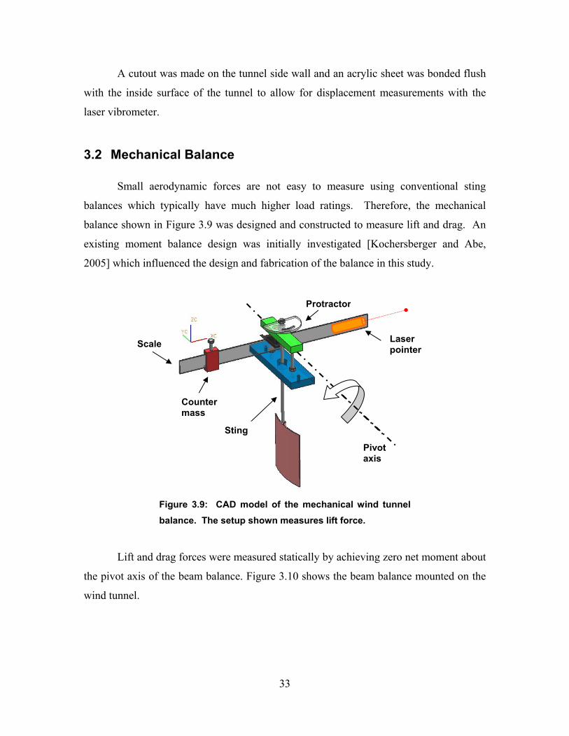
3.2 Mechanical Balance

Small aerodynamic forces are not easy to measure using conventional sting

balances which typically have much higher load ratings. Therefore, the mechanical

balance shown in Figure 3.9 was designed and constructed to measure lift and drag. An

existing moment balance design was initially investigated [Kochersberger and Abe,

2005] which influenced the design and fabrication of the balance in this study.

Counter mass

Sting

Laser pointer

Pivot axis

Protractor

Scale

Figure 3.9: CAD model of the mechanical wind tunnel balance. The setup shown measures lift force.

Lift and drag forces were measured statically by achieving zero net moment about

the pivot axis of the beam balance. Figure 3.10 shows the beam balance mounted on the

wind tunnel.

33

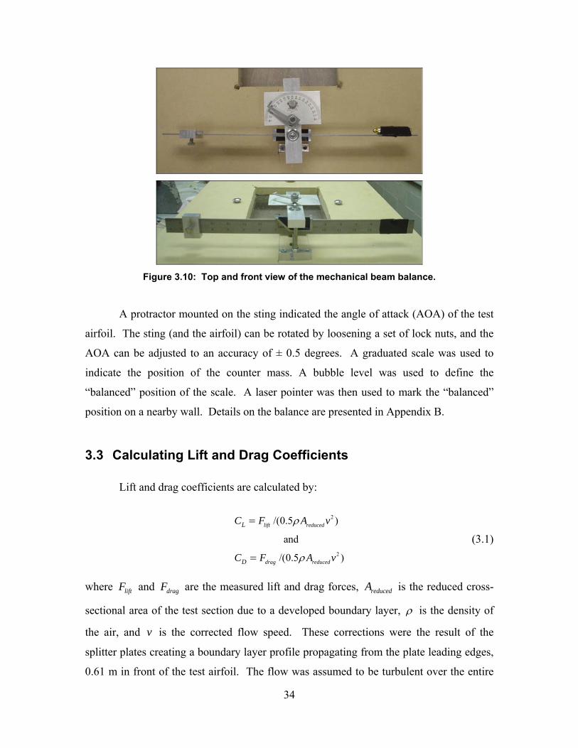
Figure 3.10: Top and front view of the mechanical beam balance.

A protractor mounted on the sting indicated the angle of attack (AOA) of the test

airfoil. The sting (and the airfoil) can be rotated by loosening a set of lock nuts, and the

AOA can be adjusted to an accuracy of ± 0.5 degrees. A graduated scale was used to

indicate the position of the counter mass. A bubble level was used to define the

“balanced” position of the scale. A laser pointer was then used to mark the “balanced”

position on a nearby wall. Details on the balance are presented in Appendix B.

3.3 Calculating Lift and Drag Coefficients

Lift and drag coefficients are calculated by:

(3.1)

2

2

/(0.5 )

and

/(0.5 )

lift reduced

drag reduced

L

D

C F A v

C F A v

ρ

ρ

=

=

where and are the measured lift and drag forces, is the reduced cross-

sectional area of the test section due to a developed boundary layer,

liftF dragF reducedA

ρ is the density of

the air, and is the corrected flow speed. These corrections were the result of the

splitter plates creating a boundary layer profile propagating from the plate leading edges,

0.61 m in front of the test airfoil. The flow was assumed to be turbulent over the entire

v

34

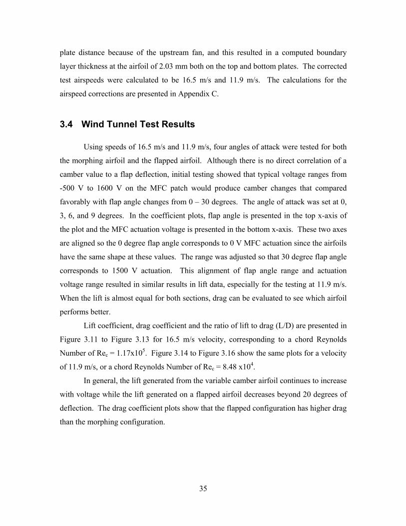
plate distance because of the upstream fan, and this resulted in a computed boundary

layer thickness at the airfoil of 2.03 mm both on the top and bottom plates. The corrected

test airspeeds were calculated to be 16.5 m/s and 11.9 m/s. The calculations for the

airspeed corrections are presented in Appendix C.

3.4 Wind Tunnel Test Results

Using speeds of 16.5 m/s and 11.9 m/s, four angles of attack were tested for both

the morphing airfoil and the flapped airfoil. Although there is no direct correlation of a

camber value to a flap deflection, initial testing showed that typical voltage ranges from

-500 V to 1600 V on the MFC patch would produce camber changes that compared

favorably with flap angle changes from 0 – 30 degrees. The angle of attack was set at 0,

3, 6, and 9 degrees. In the coefficient plots, flap angle is presented in the top x-axis of

the plot and the MFC actuation voltage is presented in the bottom x-axis. These two axes

are aligned so the 0 degree flap angle corresponds to 0 V MFC actuation since the airfoils

have the same shape at these values. The range was adjusted so that 30 degree flap angle

corresponds to 1500 V actuation. This alignment of flap angle range and actuation

voltage range resulted in similar results in lift data, especially for the testing at 11.9 m/s.

When the lift is almost equal for both sections, drag can be evaluated to see which airfoil

performs better.

Lift coefficient, drag coefficient and the ratio of lift to drag (L/D) are presented in

Figure 3.11 to Figure 3.13 for 16.5 m/s velocity, corresponding to a chord Reynolds

Number of Rec = 1.17x105. Figure 3.14 to Figure 3.16 show the same plots for a velocity

of 11.9 m/s, or a chord Reynolds Number of Rec = 8.48 x104.

In general, the lift generated from the variable camber airfoil continues to increase

with voltage while the lift generated on a flapped airfoil decreases beyond 20 degrees of

deflection. The drag coefficient plots show that the flapped configuration has higher drag

than the morphing configuration.

35

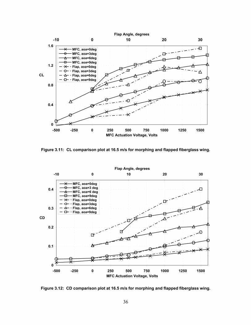
0

0.4

0.8

1.2

1.6

-500 -250 0 250 500 750 1000 1250 1500MFC Actuation Voltage, Volts

CL

-10 0 10 20 30Flap Angle, degrees

MFC, aoa=0degMFC, aoa=3degMFC, aoa=6degMFC, aoa=9degFlap, aoa=0degFlap, aoa=3degFlap, aoa=6degFlap, aoa=9deg

Figure 3.11: CL comparison plot at 16.5 m/s for morphing and flapped fiberglass wing.

0

0.1

0.2

0.3

0.4


CD


MFC, aoa=0degMFC, aoa=3 degMFC, aoa=6 degMFC, aoa=9degFlap, aoa=0degFlap, aoa=3degFlap, aoa=6degFlap, aoa=9deg

Figure 3.12: CD comparison plot at 16.5 m/s for morphing and flapped fiberglass wing.

36

2

4

6

8

10

12

-500 -250 0 250 500 750 1000 1250 1500

MFC Actuation Voltage, Volts

L/D


MFC, aoa=3 degMFC, aoa=6 degMFC, aoa=9degFlap, aoa=3degFlap, aoa=6degFlap, aoa=9deg

Figure 3.13: L/D comparison plot at 16.5 m/s for morphing and flapped fiberglass wing.

0

0.4

0.8

1.2

1.6

-500 -250 0 250 500 750 1000 1250 1500


CL

-10 0 10 20 30

Flap Angle, degrees


Figure 3.14: CL comparison plot at 11.9 m/s for morphing and flapped fiberglass wing.

37

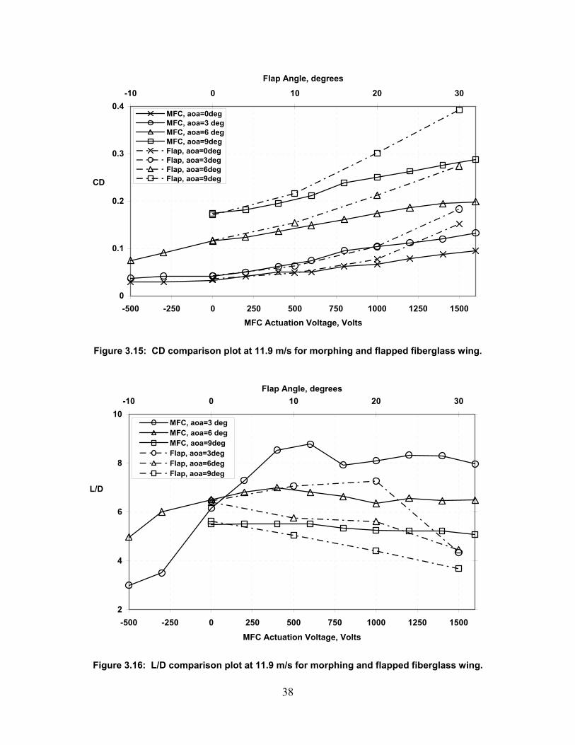
0

0.1

0.2

0.3

0.4


CD

-10 0 10 20 30

Flap Angle, degrees


Figure 3.15: CD comparison plot at 11.9 m/s for morphing and flapped fiberglass wing.

2

4

6

8

10

-500 -250 0 250 500 750 1000 1250 1500


L/D


MFC, aoa=3 degMFC, aoa=6 degMFC, aoa=9degFlap, aoa=3degFlap, aoa=6degFlap, aoa=9deg

Figure 3.16: L/D comparison plot at 11.9 m/s for morphing and flapped fiberglass wing.

38

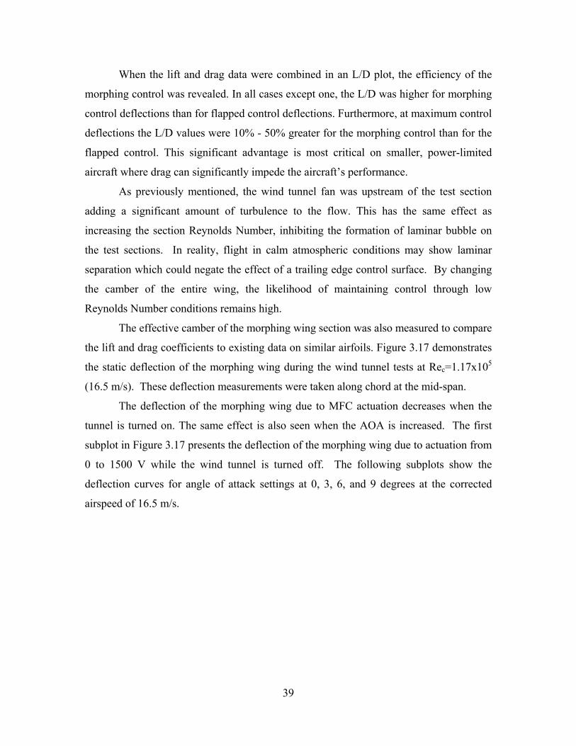
When the lift and drag data were combined in an L/D plot, the efficiency of the

morphing control was revealed. In all cases except one, the L/D was higher for morphing

control deflections than for flapped control deflections. Furthermore, at maximum control

deflections the L/D values were 10% - 50% greater for the morphing control than for the

flapped control. This significant advantage is most critical on smaller, power-limited

aircraft where drag can significantly impede the aircraft’s performance.

As previously mentioned, the wind tunnel fan was upstream of the test section

adding a significant amount of turbulence to the flow. This has the same effect as

increasing the section Reynolds Number, inhibiting the formation of laminar bubble on

the test sections. In reality, flight in calm atmospheric conditions may show laminar

separation which could negate the effect of a trailing edge control surface. By changing

the camber of the entire wing, the likelihood of maintaining control through low

Reynolds Number conditions remains high.

The effective camber of the morphing wing section was also measured to compare

the lift and drag coefficients to existing data on similar airfoils. Figure 3.17 demonstrates

the static deflection of the morphing wing during the wind tunnel tests at Rec=1.17x105

(16.5 m/s). These deflection measurements were taken along chord at the mid-span.

The deflection of the morphing wing due to MFC actuation decreases when the

tunnel is turned on. The same effect is also seen when the AOA is increased. The first

subplot in Figure 3.17 presents the deflection of the morphing wing due to actuation from

0 to 1500 V while the wind tunnel is turned off. The following subplots show the

deflection curves for angle of attack settings at 0, 3, 6, and 9 degrees at the corrected

airspeed of 16.5 m/s.

39

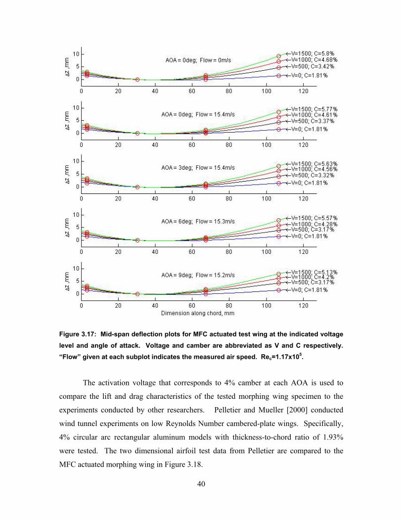
Figure 3.17: Mid-span deflection plots for MFC actuated test wing at the indicated voltage level and angle of attack. Voltage and camber are abbreviated as V and C respectively. “Flow” given at each subplot indicates the measured air speed. Rec=1.17x105.

The activation voltage that corresponds to 4% camber at each AOA is used to

compare the lift and drag characteristics of the tested morphing wing specimen to the

experiments conducted by other researchers. Pelletier and Mueller [2000] conducted

wind tunnel experiments on low Reynolds Number cambered-plate wings. Specifically,

4% circular arc rectangular aluminum models with thickness-to-chord ratio of 1.93%

were tested. The two dimensional airfoil test data from Pelletier are compared to the

MFC actuated morphing wing in Figure 3.18.

40

-0.2

0

0.2

0.4

0.6

0.8

1

1.2

1.4

-3 0 3 6 9Angle of Attack, degrees

CL, CD

12

Pelletier, Cl, Re=6e4Pelletier, Cd, Re=6e4Pelletier, Cl, Re=1.4e5Pelletier, Cd, Re=1.4e5MFC, Cl, Re=8.48e4MFC, Cd, Re=8.48e4MFC, Cl, Re=1.17e5MFC, Cd, Re=1.17e5

Figure 3.18: Comparison of lift and drag coefficients of 4% cambered 2D airfoil.

The lift and drag coefficients of the tested morphing wing are higher than what

Pelletier has reported, and this may be due to the tunnel itself. As mentioned previously,

the tunnel utilized a fan upstream of the test section which likely caused the flow to be

non-uniform and have a higher turbulence level, effectively raising its Reynolds Number.

At the time of publication, a characterization of the tunnel has not been completed, and so

the uncertainty in the measurements has not been determined. It is possible that some of

the increased lift and drag observed was also caused by the flexing of the airfoil; having

the effect of adding energy to the flow.

41

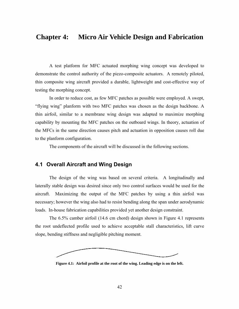
Chapter 4: Micro Air Vehicle Design and Fabrication

A test platform for MFC actuated morphing wing concept was developed to

demonstrate the control authority of the piezo-composite actuators. A remotely piloted,

thin composite wing aircraft provided a durable, lightweight and cost-effective way of

testing the morphing concept.

In order to reduce cost, as few MFC patches as possible were employed. A swept,

“flying wing” planform with two MFC patches was chosen as the design backbone. A

thin airfoil, similar to a membrane wing design was adapted to maximize morphing

capability by mounting the MFC patches on the outboard wings. In theory, actuation of

the MFCs in the same direction causes pitch and actuation in opposition causes roll due

to the planform configuration.

The components of the aircraft will be discussed in the following sections.

4.1 Overall Aircraft and Wing Design

The design of the wing was based on several criteria. A longitudinally and

laterally stable design was desired since only two control surfaces would be used for the

aircraft. Maximizing the output of the MFC patches by using a thin airfoil was

necessary; however the wing also had to resist bending along the span under aerodynamic

loads. In-house fabrication capabilities provided yet another design constraint.

The 6.5% camber airfoil (14.6 cm chord) design shown in Figure 4.1 represents

the root undeflected profile used to achieve acceptable stall characteristics, lift curve

slope, bending stiffness and negligible pitching moment.

Figure 4.1: Airfoil profile at the root of the wing. Leading edge is on the left.

42

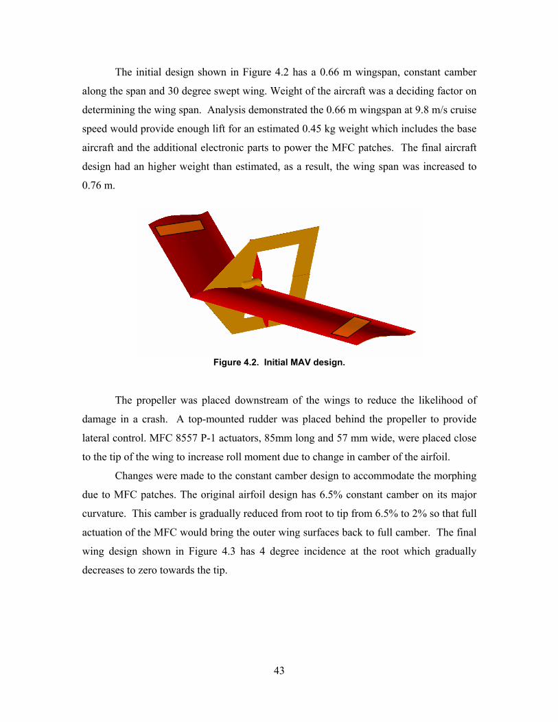
The initial design shown in Figure 4.2 has a 0.66 m wingspan, constant camber

along the span and 30 degree swept wing. Weight of the aircraft was a deciding factor on

determining the wing span. Analysis demonstrated the 0.66 m wingspan at 9.8 m/s cruise

speed would provide enough lift for an estimated 0.45 kg weight which includes the base

aircraft and the additional electronic parts to power the MFC patches. The final aircraft

design had an higher weight than estimated, as a result, the wing span was increased to

0.76 m.

Figure 4.2. Initial MAV design.

The propeller was placed downstream of the wings to reduce the likelihood of

damage in a crash. A top-mounted rudder was placed behind the propeller to provide

lateral control. MFC 8557 P-1 actuators, 85mm long and 57 mm wide, were placed close

to the tip of the wing to increase roll moment due to change in camber of the airfoil.

Changes were made to the constant camber design to accommodate the morphing

due to MFC patches. The original airfoil design has 6.5% constant camber on its major

curvature. This camber is gradually reduced from root to tip from 6.5% to 2% so that full

actuation of the MFC would bring the outer wing surfaces back to full camber. The final

wing design shown in Figure 4.3 has 4 degree incidence at the root which gradually

decreases to zero towards the tip.

43

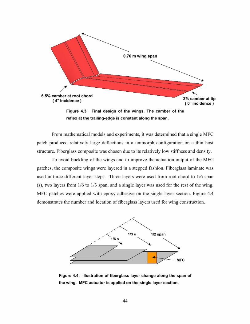
2% camber at tip ( 0° incidence )

6.5% camber at root c(

hord 4° incidence )

0.76 m wing span

Figure 4.3: Final design of the wings. The camber of the reflex at the trailing-edge is constant along the span.

From mathematical models and experiments, it was determined that a single MFC

patch produced relatively large deflections in a unimorph configuration on a thin host

structure. Fiberglass composite was chosen due to its relatively low stiffness and density.

To avoid buckling of the wings and to improve the actuation output of the MFC

patches, the composite wings were layered in a stepped fashion. Fiberglass laminate was

used in three different layer steps. Three layers were used from root chord to 1/6 span

(s), two layers from 1/6 to 1/3 span, and a single layer was used for the rest of the wing.

MFC patches were applied with epoxy adhesive on the single layer section. Figure 4.4

demonstrates the number and location of fiberglass layers used for wing construction.

Figure 4.4: Illustration of fiberglass layer change along the span of the wing. MFC actuator is applied on the single layer section.

1/2 span1/3 s1/6 s

MFC

44

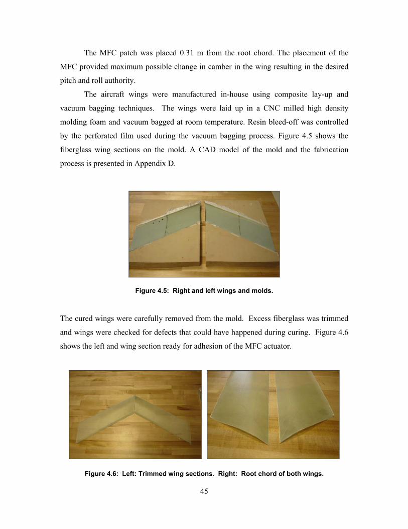
The MFC patch was placed 0.31 m from the root chord. The placement of the

MFC provided maximum possible change in camber in the wing resulting in the desired

pitch and roll authority.

The aircraft wings were manufactured in-house using composite lay-up and

vacuum bagging techniques. The wings were laid up in a CNC milled high density

molding foam and vacuum bagged at room temperature. Resin bleed-off was controlled

by the perforated film used during the vacuum bagging process. Figure 4.5 shows the

fiberglass wing sections on the mold. A CAD model of the mold and the fabrication

process is presented in Appendix D.

Figure 4.5: Right and left wings and molds.

The cured wings were carefully removed from the mold. Excess fiberglass was trimmed

and wings were checked for defects that could have happened during curing. Figure 4.6

shows the left and wing section ready for adhesion of the MFC actuator.

Figure 4.6: Left: Trimmed wing sections. Right: Root chord of both wings.

45

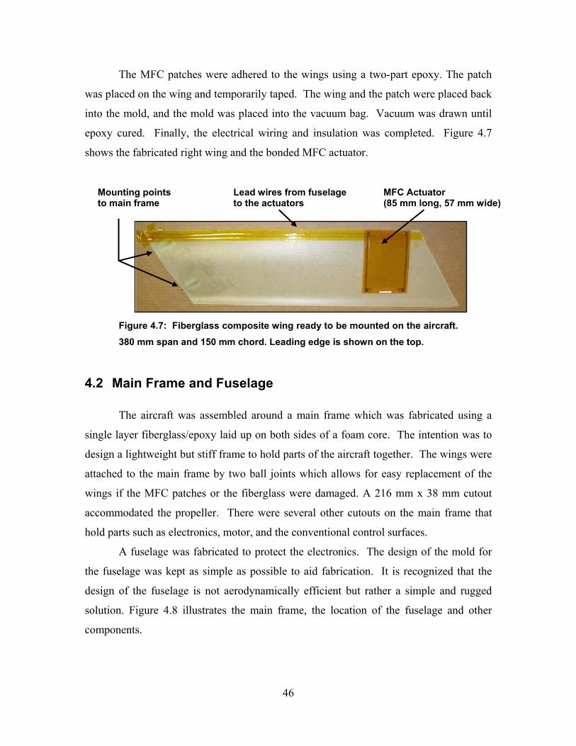
The MFC patches were adhered to the wings using a two-part epoxy. The patch

was placed on the wing and temporarily taped. The wing and the patch were placed back

into the mold, and the mold was placed into the vacuum bag. Vacuum was drawn until

epoxy cured. Finally, the electrical wiring and insulation was completed. Figure 4.7

shows the fabricated right wing and the bonded MFC actuator.

Mounting points to main frame

Figure 4.7: Fiberglass composite wing ready to be mounted on the aircraft. 380 mm span and 150 mm chord. Leading edge is shown on the top.

4.2 Main Frame and Fuselage

The aircraft was assembled around a main frame which was fabricated using a

single layer fiberglass/epoxy laid up on both sides of a foam core. The intention was to

design a lightweight but stiff frame to hold parts of the aircraft together. The wings were

attached to the main frame by two ball joints which allows for easy replacement of the

wings if the MFC patches or the fiberglass were damaged. A 216 mm x 38 mm cutout

accommodated the propeller. There were several other cutouts on the main frame that

hold parts such as electronics, motor, and the conventional control surfaces.

A fuselage was fabricated to protect the electronics. The design of the mold for

the fuselage was kept as simple as possible to aid fabrication. It is recognized that the

design of the fuselage is not aerodynamically efficient but rather a simple and rugged

solution. Figure 4.8 illustrates the main frame, the location of the fuselage and other

components.

MFC Actuator (85 mm long, 57 mm wide)

Lead wires from fuselage to the actuators

46

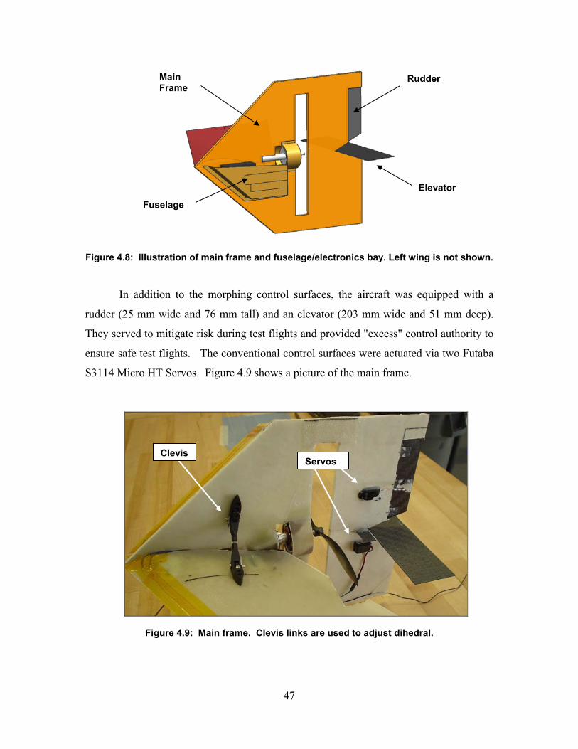
Main Frame

Rudder

Fuselage

Elevator

Figure 4.8: Illustration of main frame and fuselage/electronics bay. Left wing is not shown.

In addition to the morphing control surfaces, the aircraft was equipped with a

rudder (25 mm wide and 76 mm tall) and an elevator (203 mm wide and 51 mm deep).

They served to mitigate risk during test flights and provided "excess" control authority to

ensure safe test flights. The conventional control surfaces were actuated via two Futaba

S3114 Micro HT Servos. Figure 4.9 shows a picture of the main frame.

Clevis Servos

Figure 4.9: Main frame. Clevis links are used to adjust dihedral.

47

4.3 Electronics

The aircraft electronics are typical for model airplanes except for the power

electronics that drive the MFC actuators. Remote communication was achieved using a

72 MHz radio transmitter and receiver combination. An 11.1V Lithium-Polymer (Li-Po)

battery was used to power all electronics on-board. A brushless motor generated thrust.

Two servo actuators were used to trim yaw and pitch. MFC patches were controlled and

powered thru a series of converters. Each subsystem will be discussed in the following

sections.

4.3.1 MFC Power Electronics

Due to the nature of piezoceramics, a high voltage (HV) power supply was

necessary on-board. Two T1505 DC-DC converters from AMI Electronics were used to

supply 0 to 1500 V to the MFC patches. These converters receive 0 to 5 V input and

output 0 to 1500 V proportional to the input. Maximum power output is 1 Watt per

converter. Two RC-DC converters from CK Design Technology were used to translate

pulse-width-modulation (pwm) signals from the receiver to an analog DC signal output to

the DC-DC converters. A power booster circuit was used to amplify current output

capability of the RC-DC converter to the DC-DC converter. An experimental analysis of

the MFC power electronics is presented in Appendix D. An illustration of the electronics

can be seen in Figure 4.11.

4.3.2 Power Booster Circuit

As previously mentioned, a power booster circuit was designed and built to

amplify current output of the RC-DC converter. This is necessary because the DC-DC

converter draws about 300 mA at 4.3V input which corresponds to approximately 1500 V

output. The RC-DC converter can supply a maximum of 10 mA current. A voltage

follower circuit along with a general use power transistor allows DC-DC converter to

draw current directly from the battery instead of the RC-DC converter. The circuit is

shown in Figure 4.10.

48

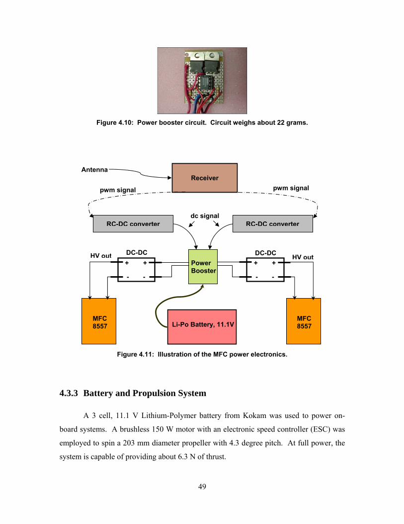
Figure 4.10: Power booster circuit. Circuit weighs about 22 grams.

Figure 4.11: Illustration of the MFC power electronics.

4.3.3 Battery and Propulsion System

A 3 cell, 11.1 V Lithium-Polymer battery from Kokam was used to power on-

board systems. A brushless 150 W motor with an electronic speed controller (ESC) was

employed to spin a 203 mm diameter propeller with 4.3 degree pitch. At full power, the

system is capable of providing about 6.3 N of thrust.

MFC 8557

+

-

+

-

HV out+

-

+

-

Li-Po Battery, 11.1V

RC-DC converter

Antenna Receiver

pwm signal pwm signal

dc signal RC-DC converter

DC-DC DC-DC HV outPower Booster

MFC 8557

49

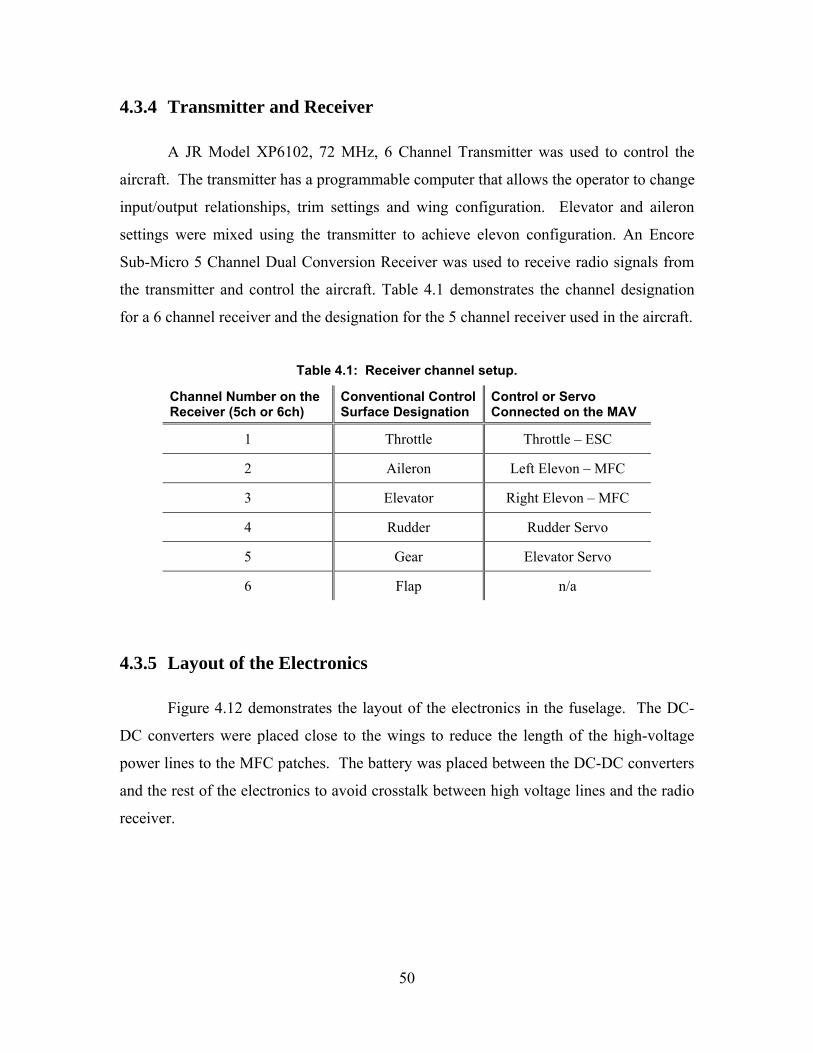
4.3.4 Transmitter and Receiver

A JR Model XP6102, 72 MHz, 6 Channel Transmitter was used to control the

aircraft. The transmitter has a programmable computer that allows the operator to change

input/output relationships, trim settings and wing configuration. Elevator and aileron

settings were mixed using the transmitter to achieve elevon configuration. An Encore

Sub-Micro 5 Channel Dual Conversion Receiver was used to receive radio signals from

the transmitter and control the aircraft. Table 4.1 demonstrates the channel designation

for a 6 channel receiver and the designation for the 5 channel receiver used in the aircraft.

Table 4.1: Receiver channel setup.

Channel Number on the Receiver (5ch or 6ch)

Conventional Control Surface Designation

Control or Servo Connected on the MAV

1 Throttle Throttle – ESC

2 Aileron Left Elevon – MFC

3 Elevator Right Elevon – MFC

4 Rudder Rudder Servo

5 Gear Elevator Servo

6 Flap n/a

4.3.5 Layout of the Electronics

Figure 4.12 demonstrates the layout of the electronics in the fuselage. The DC-

DC converters were placed close to the wings to reduce the length of the high-voltage

power lines to the MFC patches. The battery was placed between the DC-DC converters

and the rest of the electronics to avoid crosstalk between high voltage lines and the radio

receiver.

50

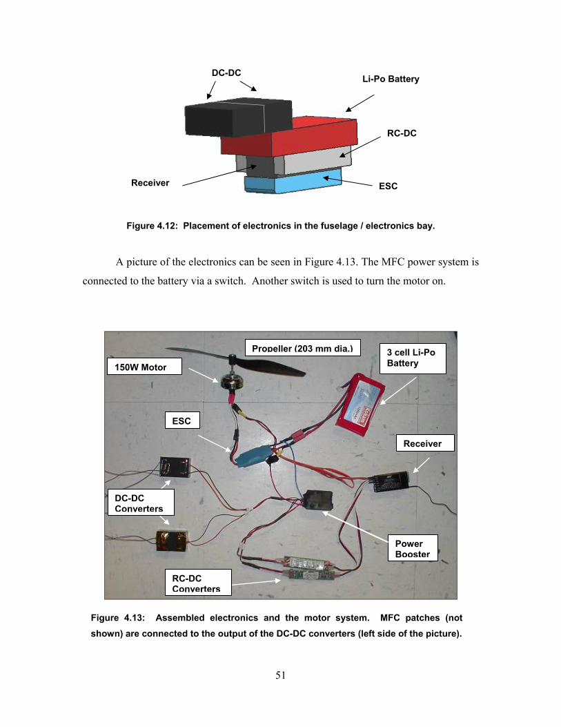
DC-DC Li-Po Battery

Receiver ESC

RC-DC

Figure 4.12: Placement of electronics in the fuselage / electronics bay.

A picture of the electronics can be seen in Figure 4.13. The MFC power system is

connected to the battery via a switch. Another switch is used to turn the motor on.

150W Motor

DC-DC Converters

RC-DC Converters

3 cell Li-Po Battery

Receiver

Propeller (203 mm dia.)

Power Booster

ESC

Figure 4.13: Assembled electronics and the motor system. MFC patches (not shown) are connected to the output of the DC-DC converters (left side of the picture).

51

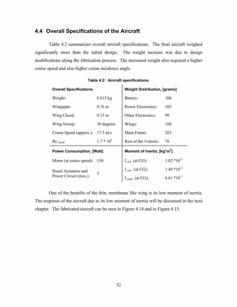
4.4 Overall Specifications of the Aircraft

Table 4.2 summarizes overall aircraft specifications. The final aircraft weighed

significantly more than the initial design. The weight increase was due to design

modifications along the fabrication process. The increased weight also required a higher

cruise speed and also higher cruise incidence angle.

Table 4.2: Aircraft specifications.

Overall Specifications Weight Distribution, [grams]

Weight: 0.815 kg Battery: 106

Wingspan: 0.76 m Power Electronics: 103

Wing Chord: 0.15 m Other Electronics: 99

Wing Sweep: 30 degrees Wings: 168

Cruise Speed (approx.): 17.5 m/s Main Frame: 263

Re chord: 1.7 * 105 Rest of the Vehicle: 76

Power Consumption, [Watt] Moment of Inertia, [kg*m2]

Motor (at cruise speed): 150 I roll (at CG): 1.02 *10-2

I yaw (at CG): 1.40 *10-2Smart Actuators and Power Circuit (max.): 3

I pitch (at CG): 6.81 *10-3

One of the benefits of the thin, membrane like wing is its low moment of inertia.

The response of the aircraft due to its low moment of inertia will be discussed in the next

chapter. The fabricated aircraft can be seen in Figure 4.14 and in Figure 4.15.

52

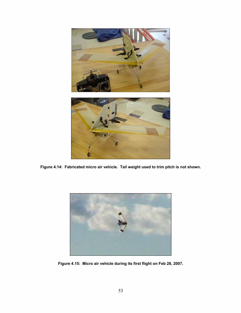
Figure 4.14: Fabricated micro air vehicle. Tail weight used to trim pitch is not shown.

Figure 4.15: Micro air vehicle during its first flight on Feb 28, 2007.

53

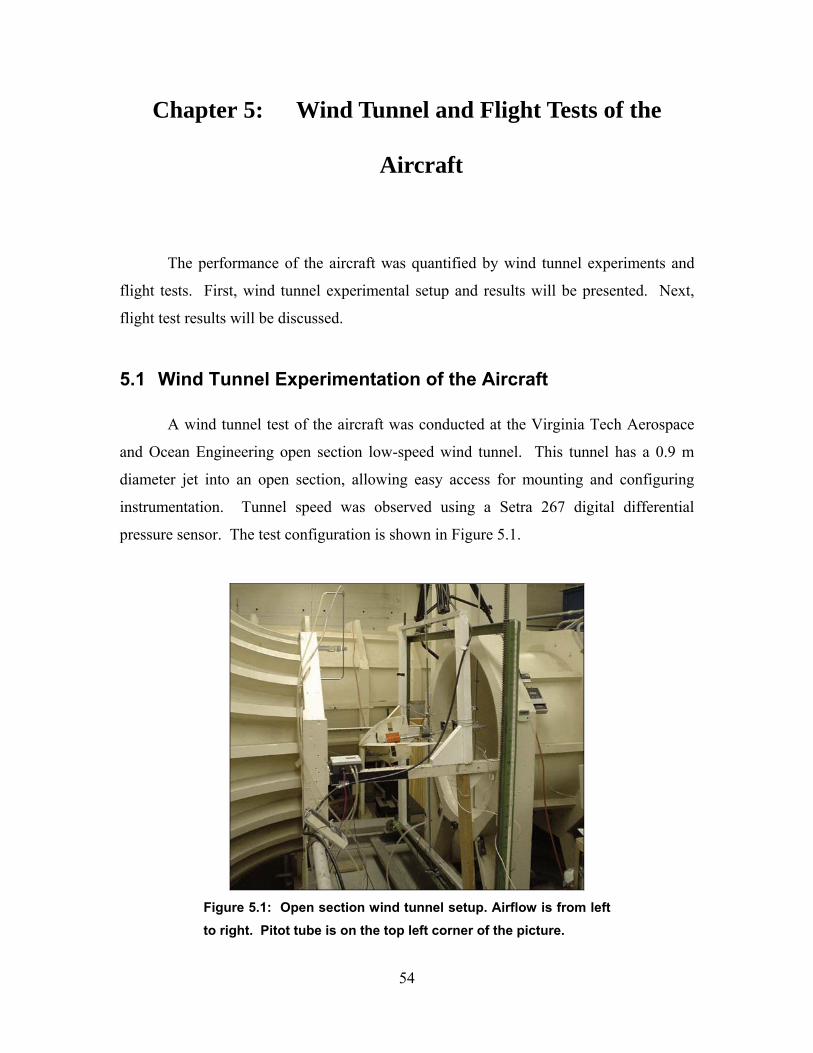
Chapter 5: Wind Tunnel and Flight Tests of the

Aircraft

The performance of the aircraft was quantified by wind tunnel experiments and

flight tests. First, wind tunnel experimental setup and results will be presented. Next,

flight test results will be discussed.

5.1 Wind Tunnel Experimentation of the Aircraft

A wind tunnel test of the aircraft was conducted at the Virginia Tech Aerospace

and Ocean Engineering open section low-speed wind tunnel. This tunnel has a 0.9 m

diameter jet into an open section, allowing easy access for mounting and configuring

instrumentation. Tunnel speed was observed using a Setra 267 digital differential

pressure sensor. The test configuration is shown in Figure 5.1.

Figure 5.1: Open section wind tunnel setup. Airflow is from left to right. Pitot tube is on the top left corner of the picture.

54

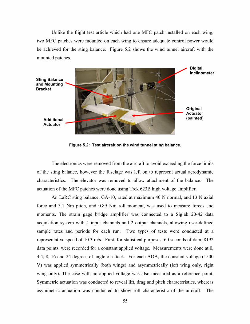
Unlike the flight test article which had one MFC patch installed on each wing,

two MFC patches were mounted on each wing to ensure adequate control power would

be achieved for the sting balance. Figure 5.2 shows the wind tunnel aircraft with the

mounted patches.

Original Actuator (painted)

Digital Inclinometer

Sting Balance and Mounting Bracket

Additional Actuator

Figure 5.2: Test aircraft on the wind tunnel sting balance.

The electronics were removed from the aircraft to avoid exceeding the force limits

of the sting balance, however the fuselage was left on to represent actual aerodynamic

characteristics. The elevator was removed to allow attachment of the balance. The

actuation of the MFC patches were done using Trek 623B high voltage amplifier.

An LaRC sting balance, GA-10, rated at maximum 40 N normal, and 13 N axial

force and 3.1 Nm pitch, and 0.89 Nm roll moment, was used to measure forces and

moments. The strain gage bridge amplifier was connected to a Siglab 20-42 data

acquisition system with 4 input channels and 2 output channels, allowing user-defined

sample rates and periods for each run. Two types of tests were conducted at a

representative speed of 10.3 m/s. First, for statistical purposes, 60 seconds of data, 8192

data points, were recorded for a constant applied voltage. Measurements were done at 0,

4.4, 8, 16 and 24 degrees of angle of attack. For each AOA, the constant voltage (1500

V) was applied symmetrically (both wings) and asymmetrically (left wing only, right

wing only). The case with no applied voltage was also measured as a reference point.

Symmetric actuation was conducted to reveal lift, drag and pitch characteristics, whereas

asymmetric actuation was conducted to show roll characteristic of the aircraft. The

55

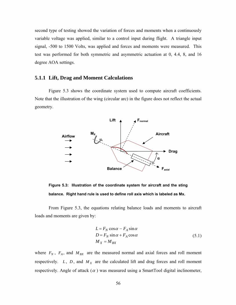
second type of testing showed the variation of forces and moments when a continuously

variable voltage was applied, similar to a control input during flight. A triangle input

signal, -500 to 1500 Volts, was applied and forces and moments were measured. This

test was performed for both symmetric and asymmetric actuation at 0, 4.4, 8, and 16

degree AOA settings.

5.1.1 Lift, Drag and Moment Calculations

Figure 5.3 shows the coordinate system used to compute aircraft coefficients.

Note that the illustration of the wing (circular arc) in the figure does not reflect the actual

geometry.

Figure 5.3: Illustration of the coordinate system for aircraft and the sting

balance. Right hand rule is used to define roll axis which is labeled as Mx.

From Figure 5.3, the equations relating balance loads and moments to aircraft

loads and moments are given by:

Lift Fnormal

cos sinsin cos

N A

N A

X BX

L F FD F FM M

α αα α

= −= +=

(5.1)

where NF , AF , and BXM are the measured normal and axial forces and roll moment

respectively. , L D , and XM are the calculated lift and drag forces and roll moment

respectively. Angle of attack (α ) was measured using a SmartTool digital inclinometer,

Faxial

Drag

MX AircraftAirflow

α

Balance

56

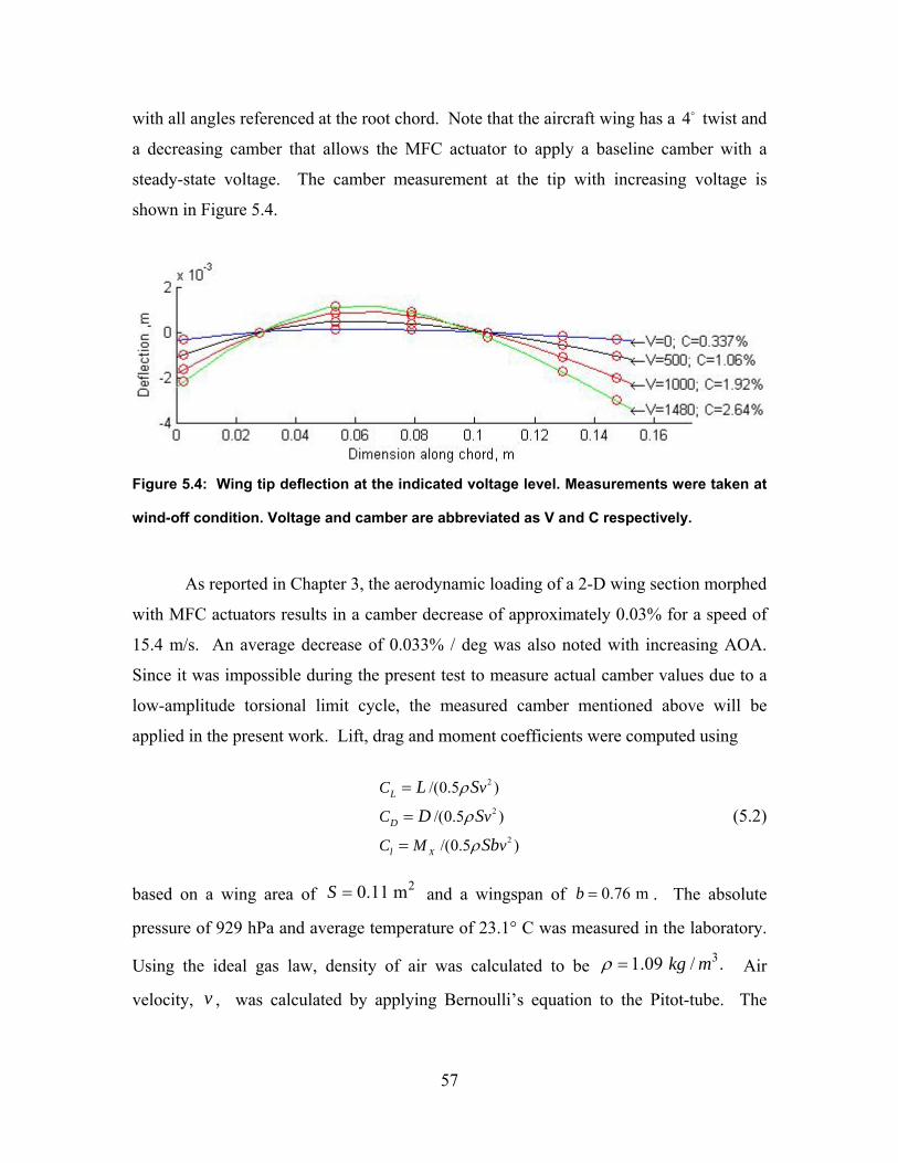
with all angles referenced at the root chord. Note that the aircraft wing has a twist and

a decreasing camber that allows the MFC actuator to apply a baseline camber with a

steady-state voltage. The camber measurement at the tip with increasing voltage is

shown in Figure 5.4.

4

Figure 5.4: Wing tip deflection at the indicated voltage level. Measurements were taken at

wind-off condition. Voltage and camber are abbreviated as V and C respectively.

As reported in Chapter 3, the aerodynamic loading of a 2-D wing section morphed

with MFC actuators results in a camber decrease of approximately 0.03% for a speed of

15.4 m/s. An average decrease of 0.033% / deg was also noted with increasing AOA.

Since it was impossible during the present test to measure actual camber values due to a

low-amplitude torsional limit cycle, the measured camber mentioned above will be

applied in the present work. Lift, drag and moment coefficients were computed using

(5.2)

2

2

2

/(0.5 )

/(0.5 )

/(0.5 )X

L

D

l

C v

C

C M v

L S

D S

Sb

ρ

ρ

ρ

=

=

=

v

based on a wing area of and a wingspan of 20.11 mS = 0.76 mb = . The absolute

pressure of 929 hPa and average temperature of 23.1° C was measured in the laboratory.

Using the ideal gas law, density of air was calculated to be Air

velocity, , was calculated by applying Bernoulli’s equation to the Pitot-tube. The

31.09 / .kg mρ =

v

57

pressure difference across the Pitot-tube was recorded with the Setra 267 pressure

transducer for each test run. An average air velocity of 10.3 m/s was calculated.

5.1.2 Uncertainty Analysis

In computing 95% confidence limits on the data, the uncertainty of measured

forces and moments had to be determined. Using AIAA Standard [1995], both precision

(P) and bias (B) errors were considered. Bias error estimates were based on repeatability

during the sting balance calibration. The following bias errors were determined using

nominal aircraft forces and moments:

0.23 N0.15 N

0.052 NmX

L

D

M

BBB

===

(5.3)

Total error in the force and moment measurements was then computed as follows:

2 2

2 2

2 2X X

L L L

D D D

M M M

U P B

U P B

U P B

= +

= +

= +X

(5.4)

The precision errors, P s, are based on 2σ (95% confidence band) values obtained from

runs that acquired 8192 values per data point over a 60 second period. In obtaining force

and moment coefficients, the uncertainties in dynamic pressure (Q), measured wing area

(S) and wingspan (b) also contribute to the overall uncertainty. Using the method of

Kline-McClintock, the force (F) and moment (M) coefficient uncertainties were

calculated. The force coefficient uncertainties become:

2 22

F

Q SFC F

U UUU CF Q S

⎛ ⎞ ⎛ ⎞⎛ ⎞= + +⎜ ⎟⎜ ⎟ ⎜ ⎟⎝ ⎠ ⎝ ⎠⎝ ⎠

(5.5)

and the moment coefficient uncertainties become:

58

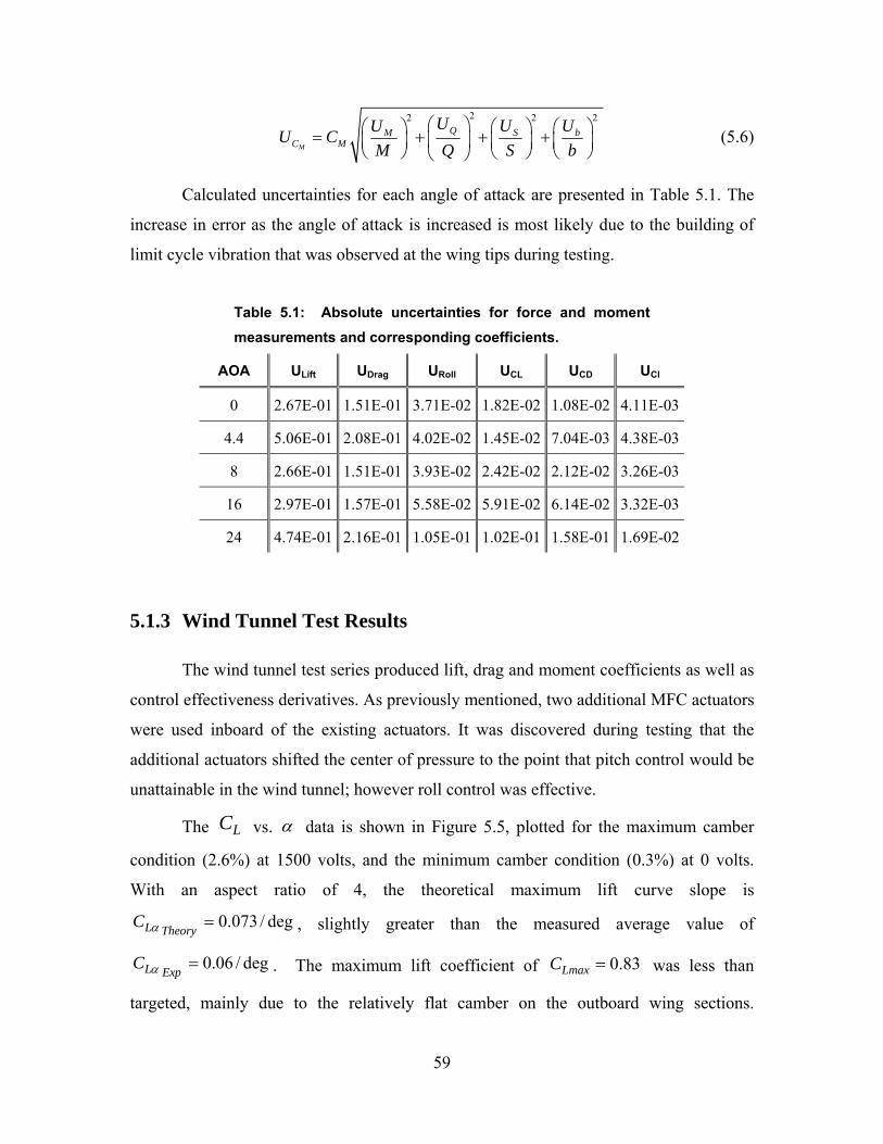
2 2 22

M

Q S bMC M

U U UUU CM Q S b

⎛ ⎞ ⎛ ⎞ ⎛ ⎞⎛ ⎞= + + +⎜ ⎟⎜ ⎟ ⎜ ⎟ ⎜ ⎟⎝ ⎠ ⎝ ⎠ ⎝ ⎠⎝ ⎠

(5.6)

Calculated uncertainties for each angle of attack are presented in Table 5.1. The

increase in error as the angle of attack is increased is most likely due to the building of

limit cycle vibration that was observed at the wing tips during testing.

Table 5.1: Absolute uncertainties for force and moment measurements and corresponding coefficients.

AOA ULift UDrag URoll UCL UCD UCl

0 2.67E-01 1.51E-01 3.71E-02 1.82E-02 1.08E-02 4.11E-03

4.4 5.06E-01 2.08E-01 4.02E-02 1.45E-02 7.04E-03 4.38E-03

8 2.66E-01 1.51E-01 3.93E-02 2.42E-02 2.12E-02 3.26E-03

16 2.97E-01 1.57E-01 5.58E-02 5.91E-02 6.14E-02 3.32E-03

24 4.74E-01 2.16E-01 1.05E-01 1.02E-01 1.58E-01 1.69E-02

5.1.3 Wind Tunnel Test Results

The wind tunnel test series produced lift, drag and moment coefficients as well as

control effectiveness derivatives. As previously mentioned, two additional MFC actuators

were used inboard of the existing actuators. It was discovered during testing that the

additional actuators shifted the center of pressure to the point that pitch control would be

unattainable in the wind tunnel; however roll control was effective.

The vs. LC α data is shown in Figure 5.5, plotted for the maximum camber

condition (2.6%) at 1500 volts, and the minimum camber condition (0.3%) at 0 volts.

With an aspect ratio of 4, the theoretical maximum lift curve slope is

, slightly greater than the measured average value of

. The maximum lift coefficient of

0.073/ degL TheoryC α =

0.06 / degL ExpC α = 0.83LmaxC = was less than

targeted, mainly due to the relatively flat camber on the outboard wing sections.

59

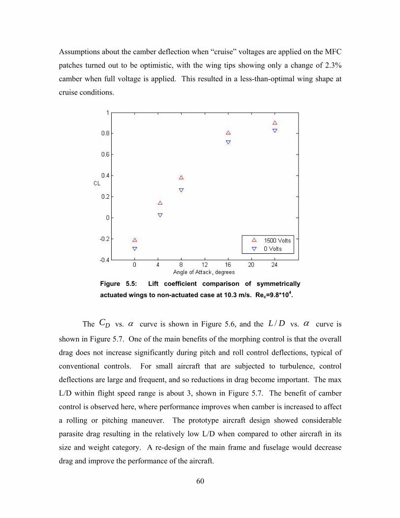
Assumptions about the camber deflection when “cruise” voltages are applied on the MFC

patches turned out to be optimistic, with the wing tips showing only a change of 2.3%

camber when full voltage is applied. This resulted in a less-than-optimal wing shape at

cruise conditions.

Figure 5.5: Lift coefficient comparison of symmetrically actuated wings to non-actuated case at 10.3 m/s. Rec=9.8*104.

The vs. DC α curve is shown in Figure 5.6, and the vs. /L D α curve is

shown in Figure 5.7. One of the main benefits of the morphing control is that the overall

drag does not increase significantly during pitch and roll control deflections, typical of

conventional controls. For small aircraft that are subjected to turbulence, control

deflections are large and frequent, and so reductions in drag become important. The max

L/D within flight speed range is about 3, shown in Figure 5.7. The benefit of camber

control is observed here, where performance improves when camber is increased to affect

a rolling or pitching maneuver. The prototype aircraft design showed considerable

parasite drag resulting in the relatively low L/D when compared to other aircraft in its

size and weight category. A re-design of the main frame and fuselage would decrease

drag and improve the performance of the aircraft.

60

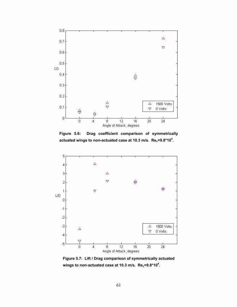
Figure 5.6: Drag coefficient comparison of symmetrically actuated wings to non-actuated case at 10.3 m/s. Rec=9.8*104.

Figure 5.7: Lift / Drag comparison of symmetrically actuated wings to non-actuated case at 10.3 m/s. Rec=9.8*104.

61

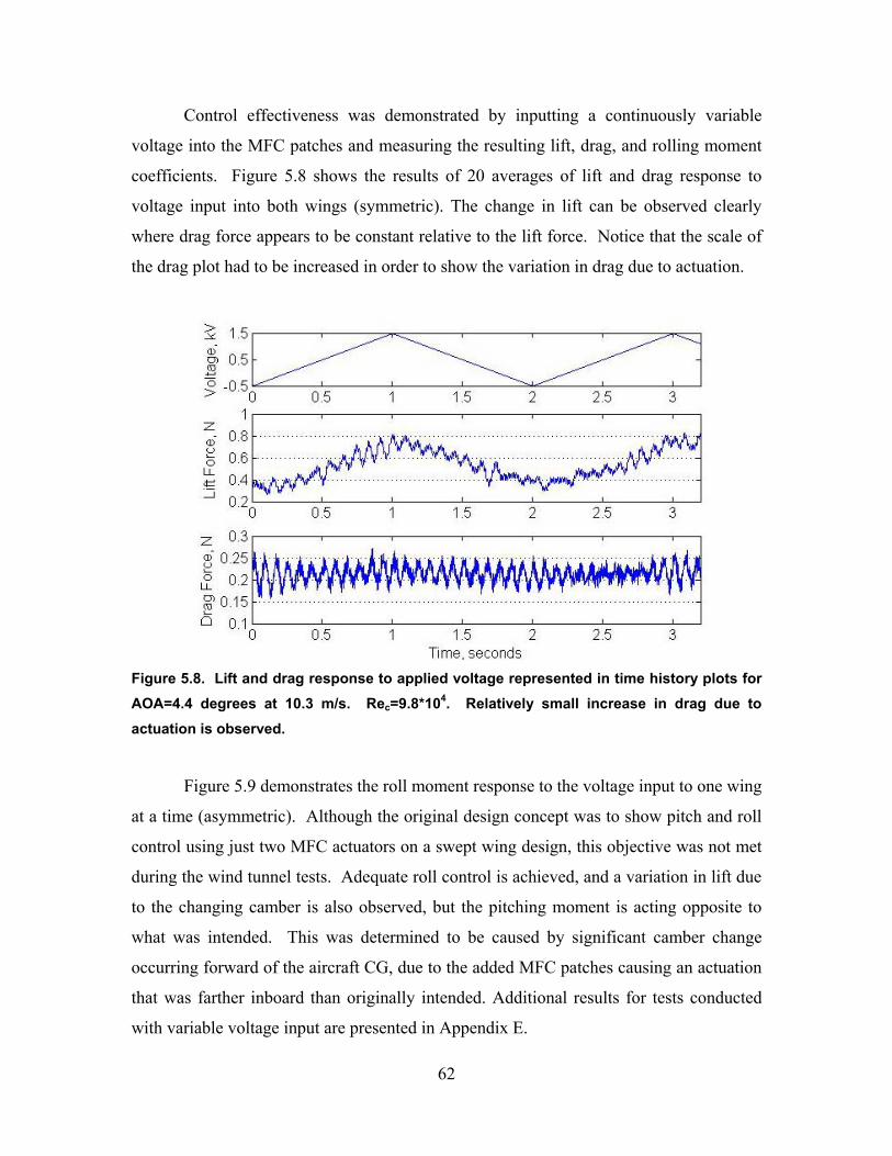
Control effectiveness was demonstrated by inputting a continuously variable

voltage into the MFC patches and measuring the resulting lift, drag, and rolling moment

coefficients. Figure 5.8 shows the results of 20 averages of lift and drag response to

voltage input into both wings (symmetric). The change in lift can be observed clearly

where drag force appears to be constant relative to the lift force. Notice that the scale of

the drag plot had to be increased in order to show the variation in drag due to actuation.

Figure 5.8. Lift and drag response to applied voltage represented in time history plots for AOA=4.4 degrees at 10.3 m/s. Rec=9.8*104. Relatively small increase in drag due to actuation is observed.

Figure 5.9 demonstrates the roll moment response to the voltage input to one wing

at a time (asymmetric). Although the original design concept was to show pitch and roll

control using just two MFC actuators on a swept wing design, this objective was not met

during the wind tunnel tests. Adequate roll control is achieved, and a variation in lift due

to the changing camber is also observed, but the pitching moment is acting opposite to

what was intended. This was determined to be caused by significant camber change

occurring forward of the aircraft CG, due to the added MFC patches causing an actuation

that was farther inboard than originally intended. Additional results for tests conducted

with variable voltage input are presented in Appendix E.

62

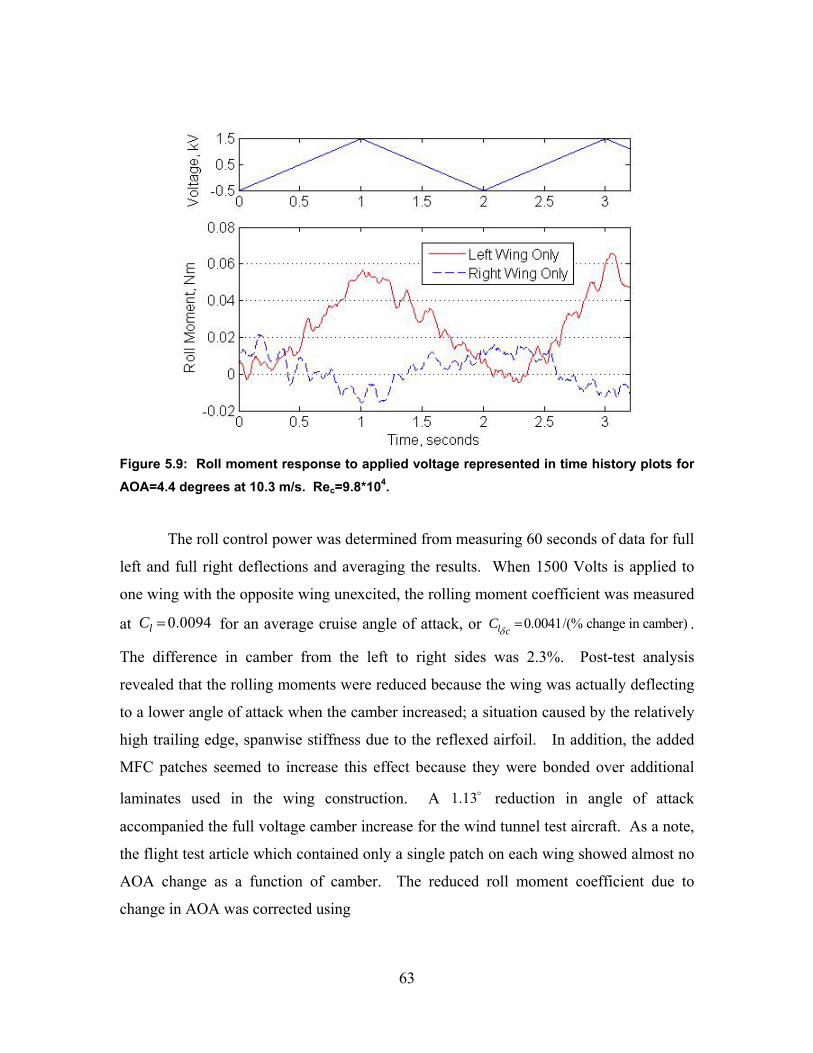
Figure 5.9: Roll moment response to applied voltage represented in time history plots for AOA=4.4 degrees at 10.3 m/s. Rec=9.8*104.

The roll control power was determined from measuring 60 seconds of data for full

left and full right deflections and averaging the results. When 1500 Volts is applied to

one wing with the opposite wing unexcited, the rolling moment coefficient was measured

at for an average cruise angle of attack, or 0.0094lC = 0.0041/(% change in camber)l cCδ = .

The difference in camber from the left to right sides was 2.3%. Post-test analysis

revealed that the rolling moments were reduced because the wing was actually deflecting

to a lower angle of attack when the camber increased; a situation caused by the relatively

high trailing edge, spanwise stiffness due to the reflexed airfoil. In addition, the added

MFC patches seemed to increase this effect because they were bonded over additional

laminates used in the wing construction. A 1. reduction in angle of attack

accompanied the full voltage camber increase for the wind tunnel test aircraft. As a note,

the flight test article which contained only a single patch on each wing showed almost no

AOA change as a function of camber. The reduced roll moment coefficient due to

change in AOA was corrected using

13

63

, Exp

MFC MFCl corrected l L

A dC C C

S bα α= + ∆ (5.7)

where area of the wing deflected by a single MFC actuator is 20.0091MFCA m= , and the

distance from the center of the active area to the root chord is . As

previously mentioned, lift curve slope is

0.31MFCd m=

0.06 / degExpLC α = and reduction in angle of

attack due to actuation is . Once the AOA effect is removed, the roll

coefficient is , and the roll coefficient control derivative becomes

.

1.13α∆ =

, 0.012l correctedC =

0.0051/ %clC

δ=

The reflexed and twisted airfoil design was originally incorporated so that the

aircraft planform could migrate from a tailed configuration (used for flight test) to a

tailless configuration (tested in the tunnel). The wind tunnel data revealed a nearly-

neutral pitching moment, and due to uncertainty it was not possible to extract accurate

pitching moment data during this experiment.

5.1.4 Dynamic Response Results

One of the benefits of a single surface, laminated wing is its low inertia. The roll

moment derivative resulting from roll rate, , can be used to determine the settling time

for a step roll command. In computing

pL

pL , the roll moment coefficient derivative, ,

is needed. This coefficient was determined from McCormick [1994] to be .

From Nelson [1998], the time response for a step roll maneuver is

lpC

0.33lpC =−

/( ) (1 )tc

cp

Lp t e

Lτδ δ−∆ = − − ∆ (5.8)

where cδ∆ is the percent change in camber, is time, and t , , andp cL Lδτ are

64

( / 2 )1 , , and

l lp cp

p x

C b u QSb C QSbL L

L Iδ

δτ =− = = .cxI

2

(5.9)

where is the air velocity and moment of inertia about the roll axis is u21.02*10x rollI I −= = kg m . The time constant of the system becomes 0.17 sτ = . The

time constant represents how fast the aircraft approaches a new steady-state condition

after being disturbed with a control input. The value calculated for the MAV is small,

representing a quick-responding aircraft.

The steady-state roll rate was not as high as desired, and this was due to the

relatively small camber change of 2.3% being affected by the MFC patches. Theoretical

steady state roll rates were determined from the non-dimensional rolling velocity, p , is

given by:

2lss c

lp

Cp bp

u Cδ cδ∆= = − (5.10)

where ssp is the steady state rolling rate, cδ∆ is the percent change in camber. The

rolling velocity is typically used to quantify an aircraft design to meet certain minimal

control requirements. For instance, fighter aircraft target a value of 0.09p= to provide

the agile handling that defines their intended use [Nelson, 1998]. Other aircraft must

meet minimum roll rates to pass the FAA airworthiness certification standards. In the

case of the morphing aircraft, the theoretical rolling velocity is 0.036p= , based on the

measured roll coefficients with angle of attack correction (discussed above).

5.2 Flight Tests

In order to validate the design, several flight attempts were made over a 1-month

period resulting in 6 successful flights. Total flight time on the aircraft is estimated to be

15 minutes. Initial flight tests have been conducted to trim roll and pitch characteristics.

During flight tests, many incidents occurred before trim points were tuned and stability

was achieved. The aircraft was virtually undamaged even after the hardest landings. It is

the experience of the author that this is not the case for vehicles with conventional control

65

surfaces. It should be pointed out that one of the valuable lessons of these trials was in

realizing the resiliency of the design. Because of the thin, flexible wing, the aircraft was

able to absorb impact energy sufficiently to survive approximately 30 incidents, most

with little or no damage to the structure.

The vehicle weight was increased due to modifications as the flight tests

continued causing a higher flight speed than originally desired. Final aircraft weight was

measured at 0.815 kg, and this resulted in a 13 m/s takeoff speed based on an initial AOA

of 13 degrees. The aircraft is hand launched at moderate running speed. Once airborne,

the aircraft accelerates to 17.5 m/s at a cruise AOA of 8 degrees.

All control inputs used up to cruise conditions were conventional: the all-moving

tail provided pitch input and the rudder provided lateral control based on the strong

dihedral stability effect due to wing sweep. Once at cruise and with little input from the

pilot, the aircraft would maintain stable flight. The elevator and rudder controls appeared

very effective, and post analysis of the flight data showed that when loss of control did

happen, it may have been due to the pilot working behind the lag of the rudder to affect

roll through roll-yaw coupling. This caused an amplification of the dutch roll mode,

finally resulting in an irrecoverable departure.

The morphing controls were operated once the plane had reached cruise

conditions. The pilot always reported not having enough control authority to fly the plane

during these trials, but this may have been an assessment biased by the relatively

effective rudder and short flight times. A limit cycle persisted in the wings from takeoff

to landing, caused by the flexibility necessary to achieve the morphing control, and this

undoubtedly reduced the control effectiveness. The wings oscillated with a symmetrical

torsion mode resulting in a trailing edge peak deflection of about 20 mm and a frequency

of about 4 Hz.

Control inputs from the operator were of interest to demonstrate the response of

the aircraft. To record the control inputs from the transmitter, a data recorder system

from Eagle Tree Systems was used. The data logger was connected to a second receiver

on ground which operated on the same frequency as the receiver on-board. Signal inputs

to left and right MFC actuated wings, rudder and elevator were recorded. The recorded

66

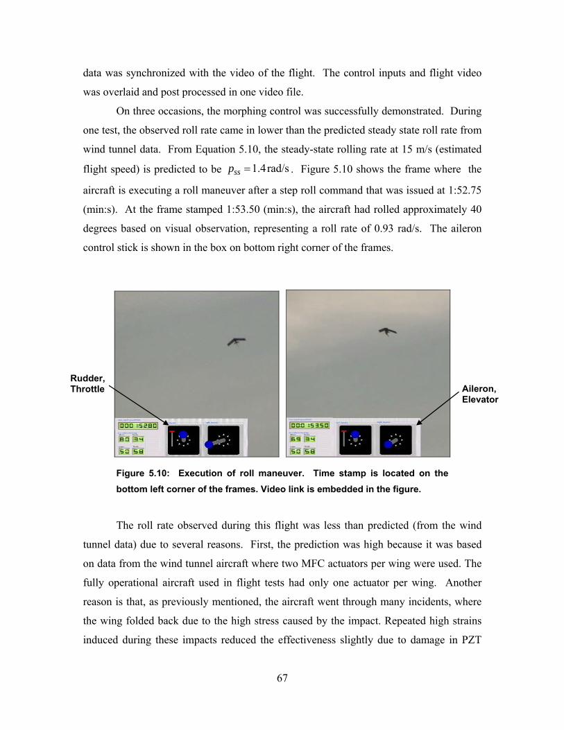
data was synchronized with the video of the flight. The control inputs and flight video

was overlaid and post processed in one video file.

On three occasions, the morphing control was successfully demonstrated. During

one test, the observed roll rate came in lower than the predicted steady state roll rate from

wind tunnel data. From Equation 5.10, the steady-state rolling rate at 15 m/s (estimated

flight speed) is predicted to be 1.4rad/sssp = . Figure 5.10 shows the frame where the

aircraft is executing a roll maneuver after a step roll command that was issued at 1:52.75

(min:s). At the frame stamped 1:53.50 (min:s), the aircraft had rolled approximately 40

degrees based on visual observation, representing a roll rate of 0.93 rad/s. The aileron

control stick is shown in the box on bottom right corner of the frames.

Rudder, Throttle Aileron,

Elevator

Figure 5.10: Execution of roll maneuver. Time stamp is located on the bottom left corner of the frames. Video link is embedded in the figure.

The roll rate observed during this flight was less than predicted (from the wind

tunnel data) due to several reasons. First, the prediction was high because it was based

on data from the wind tunnel aircraft where two MFC actuators per wing were used. The

fully operational aircraft used in flight tests had only one actuator per wing. Another

reason is that, as previously mentioned, the aircraft went through many incidents, where

the wing folded back due to the high stress caused by the impact. Repeated high strains

induced during these impacts reduced the effectiveness slightly due to damage in PZT

67

fibers and damage in the bond between the actuator and the composite wing. Finally, the

limit cycle observed during the flight test also reduced the roll authority. The amplitude

of the limit cycle was observed to be 20 mm peak-to-peak during cruise at 8° incidence.

However, only 10 mm amplitude was measured during wind tunnel tests at the 8° AOA

setting. Note that the wind tunnel tests were conducted at 10.3 m/s for the purpose of

reducing the limit cycle oscillation.

68

Chapter 6: Conclusions and Future Work

6.1 Brief Summary of Results

This study investigated the use of MFCs to control the roll and pitch maneuvers of

MAVs. In order to apply the morphing concept to an unmanned aircraft, first, the

actuation authority of MFC on thin materials was investigated. An approximation

technique, Rayleigh-Ritz model, was used to predict the deflection of unimorph

structures due to piezoelectric actuation. The model was compared to experiments. The

model revealed the behavior of the displacement of several unimorph specimens with

different host thickness. From the results, it was decided to use a single layer of

fiberglass / epoxy laminate for the morphing wing section of the experimental MAV.

Wind tunnel tests were conducted to quantify the effectiveness of MFC actuators

on a 10 cm x 10 cm circular arc test airfoil. Lift and drag coefficients were calculated and

the test results were compared to a flapped (conventional) airfoil. Results show that the

MFC actuated variable camber airfoil produced lower drag when compared to the

conventional airfoil while same lift force was produced from the two airfoils. The results

demonstrated that a thin, variable camber airfoil is an adequate control surface for flow

control for MAVs.

To demonstrate the wing morphing concept, a 0.76 m wingspan aircraft weighing

about 0.8 kg was designed and implemented using MFCs as actuators for the control

surfaces. MFCs were employed to change the camber of the wings symmetrically and

asymmetrically to cause pitch and roll respectively. A combination of amplifiers and

converters supplied the high voltage required by the MFC actuators. All systems were

powered with a Lithium-Polymer battery onboard.

The response of the MFC-actuated aircraft was quantified through wind tunnel

experimentation and flight tests. Wind tunnel tests provided lift, drag, and roll

coefficients. Maximum lift coefficient of 0.83 was measured at 24 degrees of incidence.

High parasite drag caused low lift-over-drag value of three. Using the test data, estimates

69

of flight performance were obtained. Non-dimensional rolling velocity of 0.036 was

calculated. Roll control power due to camber change, 0.0041/(% change in camber)l cC δ = ,

was adequate despite the unexpected -1.1° angle of attack change during asymmetric

actuation.

The remotely piloted experimental flight vehicle was flown using two actuators in

an elevator/aileron (elevon) configuration for a total flight time of 15 minutes. The design

demonstrated stable aerodynamic characteristics and proved the control authority of the

active materials. The flexible composite wing design provided excellent impact

resistance. The aircraft survived approximately 30 incidents, most with little or no

damage to the structure. A 0.93 rad/s roll rate was observed during the flight tests when

the MFC actuators were used. The low moment of inertia of the composite wing design

resulted in the quick-responding characteristic of the MAV.

6.2 Publications

Portions of this thesis have been presented at various professional conferences.

These works are the foundation for this thesis. Below is a list of published papers.

o Bilgen, O., Kochersberger, K., Diggs, E. C., Kurdila, A. J., Inman, D. J., “Morphing Wing Aerodynamic Control via Macro-Fiber-Composite Actuators in an Unmanned Aircraft,” AIAA-2007-2741, AIAA Infotech @ Aerospace Conference, Rohnert Park, California, May 7-10, 2007.

o Bilgen, O., Kochersberger, K., Diggs, E. C., Kurdila, A. J., Inman, D. J.,

“Morphing Wing Micro-Air-Vehicles via Macro-Fiber-Composite Actuators,” AIAA-2007-1785, 48th AIAA/ASME/ASCE/AHS/ASC Structures, Structural Dynamics, and Materials Conference, Honolulu, Hawaii, Apr. 23-26, 2007.

o Bilgen, O., Inman, D. J., Kurdila, A. J., Lind, R., “Active Materials for Wing

Morphing Micro-Air-Vehicles,” AUVSI's Unmanned Systems North America 2006 Conference, Orlando, FL, August 29-31, 2006.

70

6.3 Future Work

Future modeling and modifications on the aircraft are necessary, both for control

of the flight path and for higher frequency applications such as active flow control and

gust alleviation. MFC actuators can be used as sensors as well as actuators, and this

opens the possibility for further development of an active flow control system.

During the flight tests, symmetric limit-cycle was observed on the wings due to

their low torsional stiffness. Same oscillation was observed during the wind tunnel tests,

specifically, when the AOA was increased, the amplitude of the limit-cycle also

increased. This caused the decrease of the effectiveness of the morphing wing. During

flight tests, the cruise angle of attack was 8 degrees and cruise speed was approximated to

be 17.5 m/s. Reducing the weight of the aircraft will decrease the cruise speed and the

incidence angle, resulting in more effective morphing control.

Due to the additional MFC patches on the aircraft used in the wind tunnel,

significant reduction of incidence angle was observed. This effect reduced the pitch and

roll effectiveness of symmetric and asymmetric actuation. A stiffer leading edge and

bonding the MFC patch downstream of its current location will decrease the change in

incidence of the morphing wing. This effect has been observed on the current aircraft by

clamping a stiff beam along the leading edge. Significant increase of the trailing edge

deflection can be seen with this simple modification.

71

References

“AIAA Standard on Assessment of Experimental Uncertainty with Application to Wind Tunnel Testing,” S-071A-1995, AIAA, New York, 1995. Albertani, R., Hubner, J. P., Ifju, P. G., Lind, R., and Jackowski, J., “Experimental Aerodynamics of Micro Air Vehicles,” SAE World Aviation Congress and Exhibition, Paper 04AER-8, Nov 2004. Barlow, J. B., Rae, W. H., Pope, A., Low-Speed Wind Tunnel Testing, Wiley-Interscience; 3 Sub edition, February 22, 1999. Bartley-Cho’, J. D., Wang’, D. P., West, M. N., “Development, Control, and Test Results of High-Rate, Hingeless Trailing Edge Control Surface for the Smart Wing Phase 2 Wind Tunnel Model,” Smart Structures and Materials 2002: Industrial and Commercial Applications of Smart Structures Technologies, Proceedings of SPIE, Vol. 4698, 2002. Garcia, H. M., Abdulrahim, M., Lind, R., “Roll Control for a Micro Air Vehicle Using Active Wing Morphing,” AIAA 2003~5347. Hagood, N. W., Bent, A. A., “Development of Piezoelectric Fiber Composites for Structural Actuation,” 34th AIAA/ASME/ASCE/AHS/ASC Structures, Structural Dynamics and Materials Conference, La Jolla, CA, 1993, AIAA Paper No. 93-1717-CP, pp.3625-3638. Hagood, N. W., Kindel, R., Ghandi, K., and Gaudenzi, P., “Improving Transverse Actuation using Interdigitated Surface Electrodes,” SPIE Paper No. 1917-25, 1993 North American Conference on Smart Structures and Materials, Albuquerque, NM, pp. 341-352. High, J. W. and Wilkie, W. K., “Method of Fabricating NASA-Standard Macro-Fiber Composite Piezoelectric Actuators,” NASA/TM-2003-212427, ARL-TR-2833. Hoerner, S. F., Fluid Dynamic Lift, published by Mrs. Liselotte A. Hoerner, 1975, Hoerner Fluid Dynamics, P.O. Box 342, Brick Town, N.J. 08723, Chap. 2. Hoffman, R. J., “Free-Flight Models,” Model Aeronautics Made Painless, Published by the Author, 1955, pp. 21-22. Hyer, M. W., “Calculations of the Room-Temperature Shapes of Unsymmetric Laminates,” Journal of Composite Materials, Vol. 15, Jul. 1981, pp. 296-310.

72

Hyer, M. W., Stress Analysis of Fiber-Reinforced Composite Materials, WCB / McGraw Hill, New York, 1998.

Ifju, P. G., Ettinger, S., Jenkins, D. A., & Martinez, L., “Composite Materials for Micro Air Vehicles,” SAMPE Annual Conference, Long Beach CA, May 6-10, 2001.

Ifju, P. G., Jenkins, D. A., Ettinger, S., Lian, Y., Shyy, W., and Waszak, M. R., “Flexible-Wing-Based Micro Air Vehicles,” AIAA Annual Conference, AIAA-2002-0705. January 2002.

Inman, D. J., Cudney, H. H., “Structural and Machine Design Using Piezoceramic Materials: A Guide for Structural Design Engineers,” Final Report to NASA Langley Research Center, NASA Grant Number NAG-1-1998, April 30, 2000. Jha, A. K., Kudva, J. N., “Morphing Aircraft Concepts, Classifications, and Challenges”, Proceedings of SPIE Vol. 5388, 2004. Jones, R. M., Mechanics of Composite Materials, 2nd edition, Taylor & Francis, Inc. Philelphia, PA, 1999. Kim, D. K., Han, J. H., “Smart Flapping Wing using Macro-Fiber Composite Actuators,” Proceedings of SPIE Vol.6173 61730F, pp. 1-9, 2006. Kochersberger, K., Abe, C., “A Novel, Low Reynolds Number Moment Balance Design for Micro Air Vehicle Research,” AIAA-2005-4759, 35th AIAA Fluid Dynamics Conference and Exhibit, Toronto, Ontario, June 6-9, 2005

Lloyd, J. M., “Electrical Properties of Macro-Fiber Composite Actuators and Sensors,” M.S. Thesis, Mechanical Engineering Dept., Virginia Tech, Blacksburg, VA, June 22nd, 2004. McCormick, B., Aerodynamics, Aeronautics and Flight Mechanics, 2nd Edition, John Wiley and Sons, New York, NY, 1994, p. 527. Moses, R. W., Weisman, C. D., Bent, A. A., and Pizzochero, A. E., “Evaluation of New Actuators in a Buffet Loads Environment,” SPIE 8th Annual International Symposium on Smart Structures and Materials, Newport Beach, CA, 2001. Mueller, T. J., Burns, T. F., “Experimental Studies of the Eppler 61 Airfoil at Low Reynolds Numbers,” AIAA Paper 82-0345, Jan. 1982. Nelson, R.C., Flight Stability and Automatic Control, 2nd Edition, McGraw Hill, Boston, MA, 1998, p.182.

73

Pelletier, A., Mueller, T. J., “Low Reynolds Number Aerodynamics of Low-Aspect-Ratio, Thin/Flat/Cambered-Plate Wings,” Journal of Aircraft, Vol. 37, No. 5, September-October 2000.

Prandtl, L., “Mutual Influence of Wings and Propeller,” NACA Technical Notes No. 74, Extract from the First of the Gottingen Aerodynamic Laboratory, Chapter IV, Sec. 6, December 1921.

Ruggiero, E., Park, G., Inman, D. J. and Wright, J., “Multi-Input, Multi-Output Modal Testing Techniques for a Gossamer Structure,” Proceedings, IMECE 02, 2002 ASME IMECE Adaptive Structures Symposium, November 17-22, New Orleans, LA. Schultz, M. R., “Use of Piezoelectric Actuators to Effect Snap-Through Behavior of Unsymmetric Composite Laminates”, Ph.D. Dissertation, Engineering Science and Mechanics Dept, Virginia Tech, Blacksburg, VA, April 17th, 2003. Schultz, M. R., Hyer, M. W., “A Morphing Concept Based on Unsymmetric Composite Laminates and Piezoceramic MFC Actuators,” 45th AIAA/ASME/ASCE/AHS/ASC Structures, Structural Dynamics & Materials Conference, 2004.

Smith, R., Smart Material Systems: Model Development, Siam, Philadelphia, 2005, page xiii. Sodano, H. A., Park, G., and Inman, D. J., “The Use of Macro-Fiber Composites in Structural Vibration Applications,” Mechanical Systems and Signal Processing, 2003. Torres, G. E., “Aerodynamics of Low Aspect Ratio Wings at Low Reynolds Numbers with Applications to Micro Air Vehicle Design,” Ph.D. Dissertation, Aerospace and Mechanical Engineering Dept., University of Notre Dame, Indiana, April 2002.

Waszak, M. R., Jenkins, L. N., Ifju, P. G., “Stability and Control Properties of an Aeroelastic Fixed Wing Micro Aerial Vehicle,” AIAA-2001-4005. Wilkie, W. K., Bryant, G. R., High, J. W., “Low-Cost Piezocomposite Actuator for Structural Control Applications,” SPIE 7th Annual International Symposium on Smart Structures and Materials, Newport Beach, CA, 2000.

Wilkie, W. K., Inman, D. J., Lloyd, J. M., High, J. W., “Anisotropic Laminar Piezocomposite Actuator Incorporating Machined PMN-PT Single-crystal Fibers,” Journal Of Intelligent Material Systems And Structures, Vol. 17, January 2006. Williams, R. B., “Nonlinear Mechanical and Actuation Characterization of Piezoceramic Fiber Composites,” Ph.D. Dissertation, Mechanical Engineering Dept., Virginia Tech, Blacksburg, VA, March 22nd, 2004. Wright Brothers, Wikipedia search, [http://en.wikipedia.org/wiki/Wright_brothers].

74

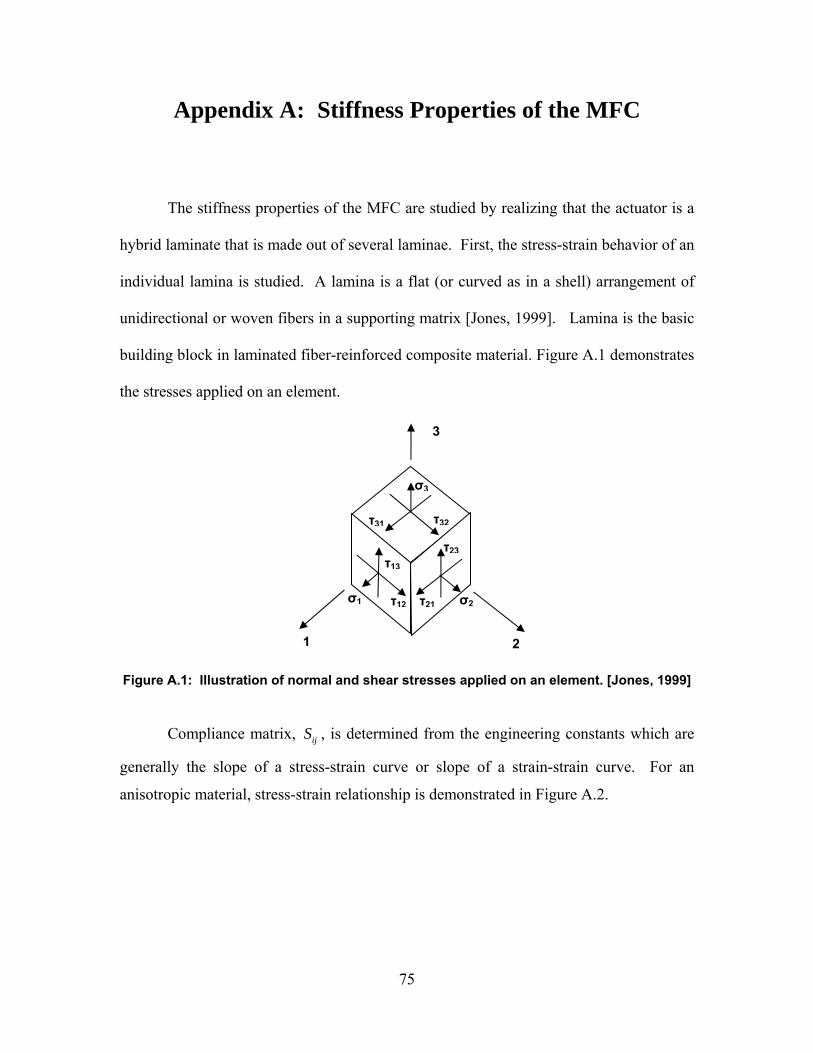
Appendix A: Stiffness Properties of the MFC

The stiffness properties of the MFC are studied by realizing that the actuator is a

hybrid laminate that is made out of several laminae. First, the stress-strain behavior of an

individual lamina is studied. A lamina is a flat (or curved as in a shell) arrangement of

unidirectional or woven fibers in a supporting matrix [Jones, 1999]. Lamina is the basic

building block in laminated fiber-reinforced composite material. Figure A.1 demonstrates

the stresses applied on an element.

3

σ3

τ32τ31

τ23τ13

σ1 σ2τ12 τ21

1 2

Figure A.1: Illustration of normal and shear stresses applied on an element. [Jones, 1999]

Compliance matrix, , is determined from the engineering constants which are

generally the slope of a stress-strain curve or slope of a strain-strain curve. For an

anisotropic material, stress-strain relationship is demonstrated in Figure A.2.

ijS

75

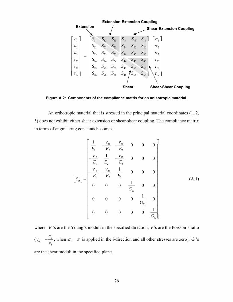
76

Extension-Extension Coupling Extension Shear-Extension Coupling

11 12 13 14 15 161 1

12 22 23 24 25 262 2

13 23 33 34 35 363 3

14 24 34 44 45 4623 23

15 25 35 45 55 5631 31

16 26 36 46 56 6612 12

S S S S S SS S S S S SS S S S S SS S S S S SS S S S S SS S S S S S

ε σε σε σγ τγ τγ τ

⎡ ⎤⎡ ⎤ ⎡ ⎤⎢ ⎥⎢ ⎥ ⎢ ⎥⎢ ⎥⎢ ⎥ ⎢ ⎥⎢ ⎥⎢ ⎥ ⎢ ⎥

= ⎢ ⎥⎢ ⎥ ⎢ ⎥⎢ ⎥⎢ ⎥ ⎢ ⎥⎢ ⎥⎢ ⎥ ⎢ ⎥⎢ ⎥⎢ ⎥ ⎢ ⎥

⎢ ⎥ ⎢ ⎥⎢ ⎥⎣ ⎦ ⎣ ⎦⎣ ⎦

Shear Shear-Shear Coupling

Figure A.2: Components of the compliance matrix for an anisotropic material.

An orthotropic material that is stressed in the principal material coordinates (1, 2,

3) does not exhibit either shear extension or shear-shear coupling. The compliance matrix

in terms of engineering constants becomes:

3121

1 2 3

3212

1 2 3

13 23

1 2 3

23

31

12

1 0 0 0

1 0 0 0

1 0 0 0

10 0 0 0 0

10 0 0 0 0

10 0 0 0 0

ij

vvE E E

vvE E Ev vE E E

S

G

G

G

⎡ ⎤− −⎢ ⎥⎢ ⎥⎢ ⎥− −⎢ ⎥⎢ ⎥⎢ ⎥− −⎢ ⎥⎢⎡ ⎤ =⎣ ⎦ ⎢⎢ ⎥⎢ ⎥⎢ ⎥⎢ ⎥⎢ ⎥⎢ ⎥⎢ ⎥⎢ ⎥⎣ ⎦

⎥⎥

(A.1)

where E ’s are the Young’s moduli in the specified direction, ’s are the Poisson’s ratio

(

v

jij

i

vεε

= − , when iσ σ= is applied in the i-direction and all other stresses are zero), G ’s

are the shear moduli in the specified plane.

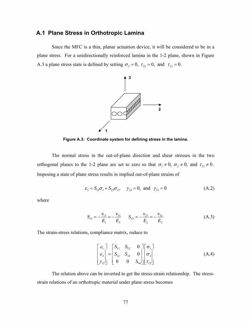
A.1 Plane Stress in Orthotropic Lamina

Since the MFC is a thin, planar actuation device, it will be considered to be in a

plane stress. For a unidirectionally reinforced lamina in the 1-2 plane, shown in Figure

A.3 a plane stress state is defined by setting 3 23 310, 0, and 0σ τ τ= = = .

Figure A.3: Coordinate system for defining stress in the lamina.

The normal stress in the out-of-plane direction and shear stresses in the two

orthogonal planes to the 1-2 plane are set to zero so that 1 2 120, 0, and 0σ σ τ≠ ≠ ≠ .

Imposing a state of plane stress results in implied out-of-plane strains of

3 13 1 23 2 23 31, 0, andS S 0ε σ σ γ γ= + = = (A.2)

where

13 31 23 3213 23

1 3 2

v v v vS S3E E E

= − = − = − = −E

1

2

(A.3)

The strain-stress relations, compliance matrix, reduce to

1 11 12

2 12 22

12 66 12

00

0 0

S SS S

S

ε σε σγ τ

⎡ ⎤ ⎡ ⎤ ⎡ ⎤⎢ ⎥ ⎢ ⎥ ⎢ ⎥=⎢ ⎥ ⎢ ⎥ ⎢ ⎥⎢ ⎥ ⎢ ⎥ ⎢ ⎥⎣ ⎦ ⎣ ⎦ ⎣ ⎦

(A.4)

The relation above can be inverted to get the stress-strain relationship. The stress-

strain relations of an orthotropic material under plane stress becomes

3

2

1

77

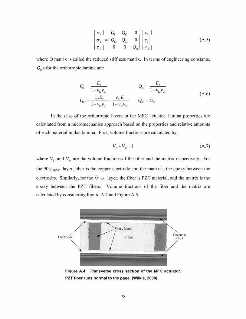
1 11 12

2 12 22

12 66 12

00

0 0

Q QQ Q

Q

1

2

σ εσ ετ γ

⎡ ⎤ ⎡ ⎤ ⎡ ⎤⎢ ⎥ ⎢ ⎥ ⎢ ⎥=⎢ ⎥ ⎢ ⎥ ⎢ ⎥⎢ ⎥ ⎢ ⎥ ⎢ ⎥⎣ ⎦ ⎣ ⎦ ⎣ ⎦

(A.5)

where Q matrix is called the reduced stiffness matrix. In terms of engineering constants,

s for the orthotropic lamina are: ijQ

1 211 22

12 21 12 21

12 2 21 112 66 12

12 21 12 21

1 1

1 1

E EQ Qv v v v

v E v EQ Qv v v v

= =− −

= = =− −

G (A.6)

In the case of the orthotropic layers in the MFC actuator, lamina properties are

calculated from a micromechanics approach based on the properties and relative amounts

of each material in that lamina. First, volume fractions are calculated by:

1f mV V+ = (A.7)

where fV and are the volume fractions of the fiber and the matrix respectively. For

the 90°

mV

Copper layer, fiber is the copper electrode and the matrix is the epoxy between the

electrodes. Similarly, for the 0° PZT layer, the fiber is PZT material, and the matrix is the

epoxy between the PZT fibers. Volume fractions of the fiber and the matrix are

calculated by considering Figure A.4 and Figure A.5.

Figure A.4: Transverse cross section of the MFC actuator. PZT fiber runs normal to the page. [Wilkie, 2000]

78

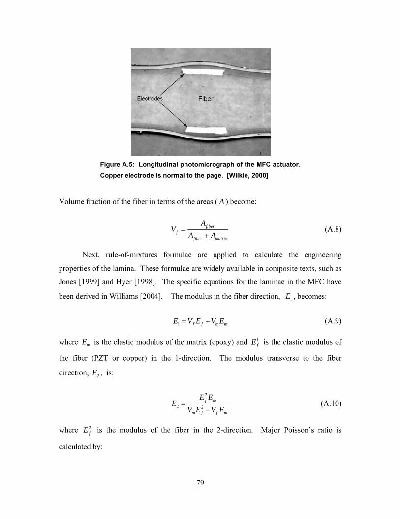
Figure A.5: Longitudinal photomicrograph of the MFC actuator. Copper electrode is normal to the page. [Wilkie, 2000]

Volume fraction of the fiber in terms of the areas ( A ) become:

fiberf

fiber matrix

AV

A A=

+ (A.8)

Next, rule-of-mixtures formulae are applied to calculate the engineering

properties of the lamina. These formulae are widely available in composite texts, such as

Jones [1999] and Hyer [1998]. The specific equations for the laminae in the MFC have

been derived in Williams [2004]. The modulus in the fiber direction, , becomes: 1E

11 f f m mE V E V E= + (A.9)

where is the elastic modulus of the matrix (epoxy) and mE 1fE is the elastic modulus of

the fiber (PZT or copper) in the 1-direction. The modulus transverse to the fiber

direction, , is: 2E

2

2 2f m

m f f m

E EE

V E V E=

+ (A.10)

where 2fE is the modulus of the fiber in the 2-direction. Major Poisson’s ratio is

calculated by:

79

1212 f f mv V v V v= + m (A.11)

where 12fv is the Poisson’s ratio of the transversely isotropic PZT fiber relating strains

induced in the 2-direction to those applied in the 1-direction of the fiber. In case of the

copper fiber, the directional superscript can be omitted where 12f copperv v= . The in-plane

shear modulus, , is: 12G

12

12 12f m

m f f m

G GG

V G V G=

+ (A.12)

where 12fG is the shear modulus in the 1-2 plane of the fiber.

A.2 Plane Stress in Isotropic Laminae

For isotropic materials, there are only two independent material constants. The

MFC has several isotropic layers such as the IsoKapton layer and the IsoAcrylic layer.

Aluminum and stainless steel, the host materials for the unimorph actuator that were used

in the experiments, are also considered isotropic. The reduced stiffness matrices for the

two isotropic host materials are calculated using the equations in this section. The

isotropic lamina can be analyzed as an orthotropic lamina by realizing and

. The strain-stress relations for these layers are:

1E E= 2

1

2

12G G=

1 11 12

2 12 11

12 11 12 12

00

0 0 2( )

S SS S

S S

ε σε σγ τ

⎡ ⎤ ⎡ ⎤ ⎡ ⎤⎢ ⎥ ⎢ ⎥ ⎢ ⎥=⎢ ⎥ ⎢ ⎥ ⎢ ⎥⎢ ⎥ ⎢ ⎥ ⎢ ⎥−⎣ ⎦ ⎣ ⎦ ⎣ ⎦

(A.13)

where

11 121 , and .vS SE E

= = − (A.14)

The stress-strain relation becomes:

80

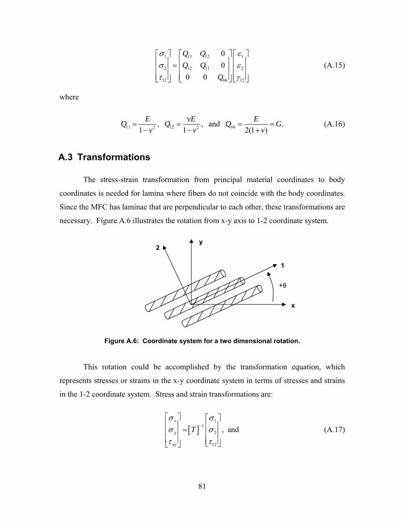
1 11 12

2 12 11

12 66 12

00

0 0

Q QQ Q

Q

1

2

σ εσ ετ γ

⎡ ⎤ ⎡ ⎤ ⎡ ⎤⎢ ⎥ ⎢ ⎥ ⎢ ⎥=⎢ ⎥ ⎢ ⎥ ⎢ ⎥⎢ ⎥ ⎢ ⎥ ⎢ ⎥⎣ ⎦ ⎣ ⎦ ⎣ ⎦

(A.15)

where

11 12 662 2, , and1 1 2(1 )

E vE EQ Q Qv v v

= = =− − +

.G= (A.16)

A.3 Transformations

The stress-strain transformation from principal material coordinates to body

coordinates is needed for lamina where fibers do not coincide with the body coordinates.

Since the MFC has laminae that are perpendicular to each other, these transformations are

necessary. Figure A.6 illustrates the rotation from x-y axis to 1-2 coordinate system.

Figure A.6: Coordinate system for a two dimensional rotation.

This rotation could be accomplished by the transformation equation, which

represents stresses or strains in the x-y coordinate system in terms of stresses and strains

in the 1-2 coordinate system. Stress and strain transformations are:

(A.17) [ ]1

12

12

, andx

y

xy

Tσ σσ στ τ

−

⎡ ⎤ ⎡ ⎤⎢ ⎥ ⎢ ⎥=⎢ ⎥ ⎢ ⎥⎢ ⎥ ⎢ ⎥⎣ ⎦⎣ ⎦

y2

1

+θ

x

81

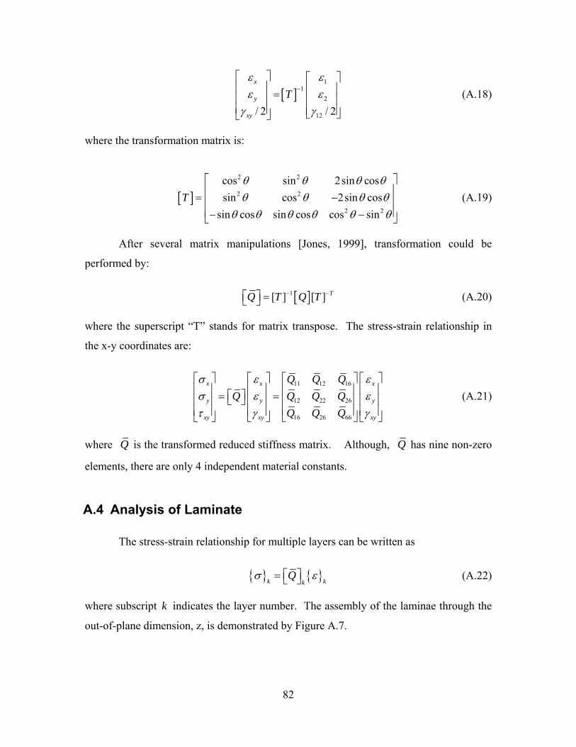
[ ]1

12

12/ 2 / 2

x

y

xy

Tε εε

γ γ

−

⎡ ⎤

ε⎡ ⎤

⎢ ⎥ ⎢ ⎥=⎢ ⎥ ⎢ ⎥⎢ ⎥ ⎢ ⎥⎣ ⎦⎣ ⎦

(A.18)

where the transformation matrix is:

[ ]2 2

2 2

2 2

cos sin 2sin cossin cos 2sin cos

sin cos sin cos cos sinT

θ θ θ θθ θ θ θ

θ θ θ θ θ

⎡ ⎤⎢ ⎥= −⎢ ⎥⎢ ⎥− −⎣ ⎦θ

(A.19)

After several matrix manipulations [Jones, 1999], transformation could be

performed by:

[ ]1[ ] [ ] TQ T Q T− −⎡ ⎤ =⎣ ⎦ (A.20)

where the superscript “T” stands for matrix transpose. The stress-strain relationship in

the x-y coordinates are:

11 12 16

12 22 26

16 26 66

x x

y y

xy xy xy

Q Q QQ Q Q Q

Q Q Q

x

y

σ ε εσ ε ετ γ γ

⎡ ⎤ ⎡ ⎤ ⎡ ⎤⎡ ⎤⎢ ⎥ ⎢ ⎥ ⎢ ⎥⎢⎡ ⎤= =⎣ ⎦⎢ ⎥ ⎢ ⎥ ⎢ ⎥⎢⎢ ⎥ ⎢ ⎥ ⎢ ⎥⎢ ⎥⎣ ⎦⎣ ⎦ ⎣ ⎦ ⎣ ⎦

⎥⎥ (A.21)

where Q is the transformed reduced stiffness matrix. Although, Q has nine non-zero

elements, there are only 4 independent material constants.

A.4 Analysis of Laminate

The stress-strain relationship for multiple layers can be written as

k kQ

kσ ε⎡ ⎤= ⎣ ⎦ (A.22)

where subscript indicates the layer number. The assembly of the laminae through the

out-of-plane dimension, z, is demonstrated by Figure A.7.

k

82

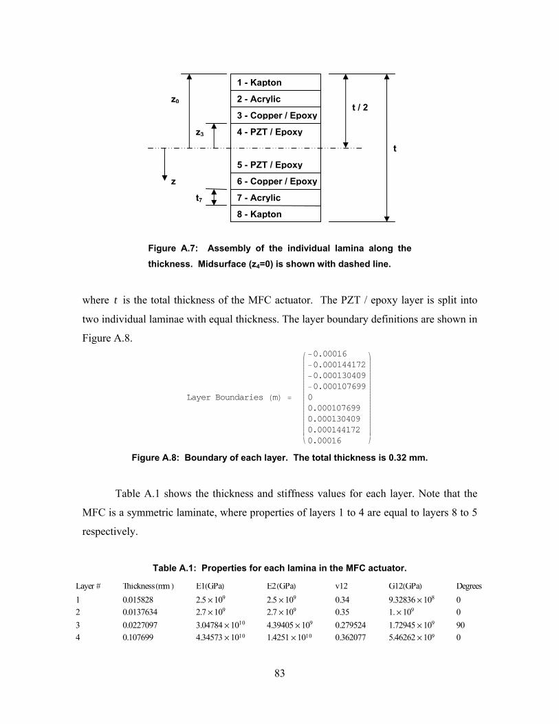
Figure A.7: Assembly of the individual lamina along the thickness. Midsurface (z4=0) is shown with dashed line.

where is the total thickness of the MFC actuator. The PZT / epoxy layer is split into

two individual laminae with equal thickness. The layer boundary definitions are shown in

Figure A.8.

t

Layer Boundaries HmL =

ijjjjjjjjjjjjjjjjjjjjjjjjjjjjj

−0.00016−0.000144172−0.000130409−0.00010769900.0001076990.0001304090.0001441720.00016

yzzzzzzzzzzzzzzzzzzzzzzzzzzzzzk

Figure A.8: Boundary of each layer. The total thickness is 0.32 mm.

Table A.1 shows the thickness and stiffness values for each layer. Note that the

MFC is a symmetric laminate, where properties of layers 1 to 4 are equal to layers 8 to 5

respectively.

Table A.1: Properties for each lamina in the MFC actuator.

Layer # ThicknessHmm L E1HGPaL E2HGPaL v12 G12HGPaL Degrees1 0.015828 2.5µ109 2.5µ109 0.34 9.32836µ108 02 0.0137634 2.7µ109 2.7µ109 0.35 1.µ109 03 0.0227097 3.04784µ1010 4.39405µ109 0.279524 1.72945µ109 904 0.107699 4.34573µ1010 1.4251µ1010 0.362077 5.46262µ109 0

1 - Kapton

2 - Acrylic

3 - Copper / Epoxy

4 - PZT / Epoxy

5 - PZT / Epoxy

t

6 - Copper / Epoxy

7 - Acrylic

8 - Kapton

z3

t / 2

t7

z

z0

83

The bond between each lamina is assumed infinitely thin and is “perfect” where

no shear occurs. As mentioned earlier, Kirchhoff hypothesis is adopted, which assumes

the line which is initially straight and perpendicular to the midplane of the laminate

remains straight and perpendicular throughout the deformation of the laminate.

Additionally, for linear elastic behavior, the Kirchhoff hypothesis can be shown to

require the strain of the laminate to vary linearly through the thickness [Jones, 1999].

Strain in the laminate becomes zε ε κ= + where ε and κ are the midplane strains and

the curvatures.

Forces ( ) and moments (N M ) are solved by integrating the stress over the

thickness of the individual lamina, and the adding together. The forces and moments

become:

11 12 16 11 12 16

12 22 26 12 22 26

16 26 66 16 26 66

11 12 16 11 12 16

12 22 26 12 22 26

16 26 66 16 26 66

x x

y y

xy xy

x x

y y

xy xy

N A A A B B BN A A A B B BN A A A B B BM B B B D D DM B B B D D DM B B B D D D

εεγκκκ

⎡ ⎤⎡ ⎤ ⎡ ⎤⎢ ⎥⎢ ⎥ ⎢ ⎥⎢ ⎥⎢ ⎥ ⎢ ⎥⎢ ⎥⎢ ⎥ ⎢ ⎥

= ⎢ ⎥⎢ ⎥ ⎢ ⎥⎢ ⎥⎢ ⎥ ⎢ ⎥⎢ ⎥⎢ ⎥ ⎢ ⎥⎢ ⎥⎢ ⎥ ⎢ ⎥

⎢ ⎥ ⎢ ⎥⎢ ⎥ ⎣ ⎦⎣ ⎦ ⎣ ⎦

(A.23)

where As, Bs and Ds are the elements of the well known ABD matrix and ε s and κ s

are the midplane strains and curvatures. Elements of the ABD matrices are defined as:

8

11

82 2

11

83 3

11

( ) ( )

1 ( ) ( )21 ( ) ( )3

ij ij k k kk

ij ij k k kk

ij ij k k kk

A Q z z

B Q z z

D Q z z

−=

−=

−=

= −

=

= −

∑

∑

∑

− (A.24)

Realizing the MFC is a symmetric laminate, the bending-extension coupling matrix (B) is

equal to zero. The inverse of ijA is the 2D analogy of the compliance matrix. Using the

definition of the compliance matrix, the four independent engineering stiffness properties

of the MFC can be calculated by:

84

211 22 12 12

22 22

26611 22 12

11

MFC MFCx x

MFC

MFC MFCy x

y

yMFC MFC

A A A AE vt A A

AA A AE Gt A t

−= =

−= =

(A.25)

A.5 References

Hyer, M. W., “Calculations of the Room-Temperature Shapes of Unsymmetric Laminates,” Journal of Composite Materials, Vol. 15, Jul. 1981, pp. 296-310. Jones, R. M., Mechanics of Composite Materials, 2nd edition, Taylor & Francis, Inc. Philelphia, PA, 1999. Wilkie, W. K., Bryant, G. R., High, J. W., “Low-Cost Piezocomposite Actuator for Structural Control Applications,” SPIE 7th Annual International Symposium on Smart Structures and Materials, Newport Beach, CA, 2000.

Williams, R. B., “Nonlinear Mechanical and Actuation Characterization of Piezoceramic Fiber Composites,” Ph.D. Dissertation, Mechanical Engineering Dept., Virginia Tech, Blacksburg, VA, March 22nd, 2004.

85

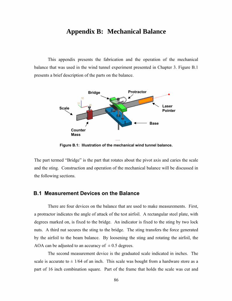
Appendix B: Mechanical Balance

This appendix presents the fabrication and the operation of the mechanical

balance that was used in the wind tunnel experiment presented in Chapter 3. Figure B.1

presents a brief description of the parts on the balance.

Figure B.1: Illustration of the mechanical wind tunnel balance.

The part termed “Bridge” is the part that rotates about the pivot axis and caries the scale

and the sting. Construction and operation of the mechanical balance will be discussed in

the following sections.

Bridge

Counter Mass

Scale Laser Pointer

Base

Protractor

B.1 Measurement Devices on the Balance

There are four devices on the balance that are used to make measurements. First,

a protractor indicates the angle of attack of the test airfoil. A rectangular steel plate, with

degrees marked on, is fixed to the bridge. An indicator is fixed to the sting by two lock

nuts. A third nut secures the sting to the bridge. The sting transfers the force generated

by the airfoil to the beam balance. By loosening the sting and rotating the airfoil, the

AOA can be adjusted to an accuracy of ± 0.5 degrees.

The second measurement device is the graduated scale indicated in inches. The

scale is accurate to ± 1/64 of an inch. This scale was bought from a hardware store as a

part of 16 inch combination square. Part of the frame that holds the scale was cut and

86

modified to attach it to the bridge. Another measuring device is the bubble level used to

indicate the “balanced” position of the scale. However a bubble level alone is not

accurate enough to locate the balanced position. A fourth device, a laser pointer, is used

to indicate the balance position more accurately.

B.2 Construction of the Balance

The structural parts of the balance were machined from 6061 aluminum utilizing

manual milling operations only. The sting was fabricated from a 10 inch long ¼-28 fully

threaded rod. The bridge was cut and squared from ½ in thick aluminum plate. Bridge

was designed to rest on two point supports. These point supports were made by cutting

¼-28 threaded rod to 2.5 in length. These rods were then ground into a fine point on one

end. The bridge had two counter-sink holes where these rods fitted. This point contact

provided low friction and also limited the motion of the balance to a rotation about the

pivot axis.

Several assumptions were made to size the components of the balance. The scale

and the sting were treated as simple beams with a uniform load distribution. All

components were treated as point masses. Error associated with these assumptions is

negligible because the test data is collected when the balance is in level position.

Leveling the balance before experiments avoided error related to the shape and load

distribution differences between different airfoils. The off-axis weight of the airfoil

created a moment which contributed to the measured lift and/or drag. When the

“leveling” was done, the offset due to the airfoil was eliminated.

B.3 Leveling the Balance and Calculating Tare Moment

Before making measurements, the “level” position for the balance had to be

found. When the tunnel is in the off condition, the counter mass is adjusted until bubble

level shows “level”. Next, laser spot is marked on a surface next to the tunnel. A wall

was chosen to make this mark on. This mark was accepted as the “balance” point for the

force measurements.

87

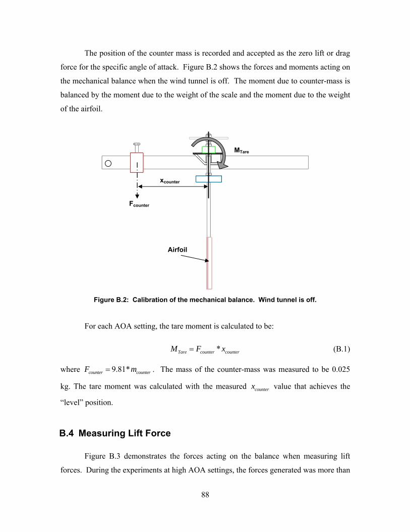
The position of the counter mass is recorded and accepted as the zero lift or drag

force for the specific angle of attack. Figure B.2 shows the forces and moments acting on

the mechanical balance when the wind tunnel is off. The moment due to counter-mass is

balanced by the moment due to the weight of the scale and the moment due to the weight

of the airfoil.

Figure B.2: Calibration of the mechanical balance. Wind tunnel is off.

For each AOA setting, the tare moment is calculated to be:

*Tare counter counterM F x= (B.1)

where . The mass of the counter-mass was measured to be 0.025

kg. The tare moment was calculated with the measured value that achieves the

“level” position.

9.81*counter counterF m=

counterx

MTare

xcounter

Fcounter

Airfoil

B.4 Measuring Lift Force

Figure B.3 demonstrates the forces acting on the balance when measuring lift

forces. During the experiments at high AOA settings, the forces generated was more than

88

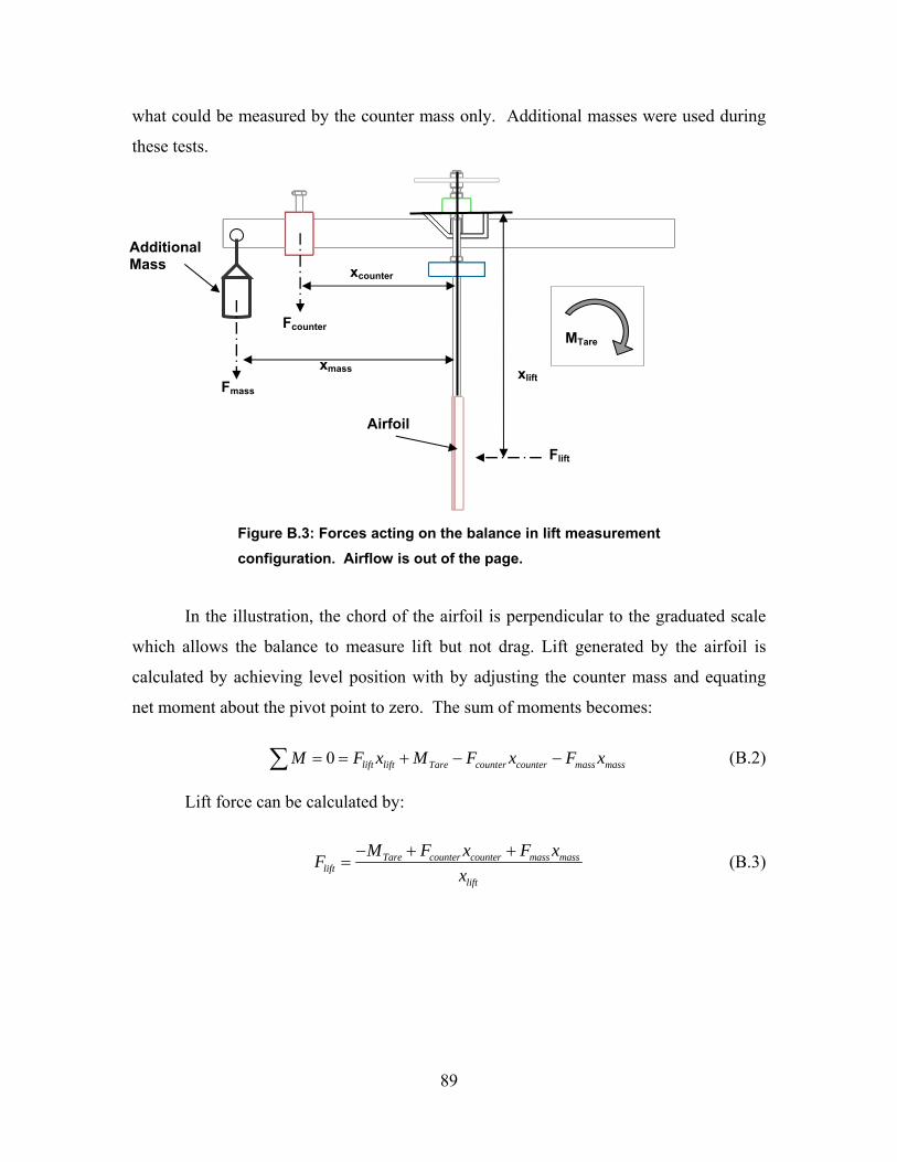
what could be measured by the counter mass only. Additional masses were used during

these tests.

Figure B.3: Forces acting on the balance in lift measurement configuration. Airflow is out of the page.

In the illustration, the chord of the airfoil is perpendicular to the graduated scale

which allows the balance to measure lift but not drag. Lift generated by the airfoil is

calculated by achieving level position with by adjusting the counter mass and equating

net moment about the pivot point to zero. The sum of moments becomes:

0 lift lift Tare counter counter mass massM F x M F x F x= = + − −∑ (B.2)

Lift force can be calculated by:

Tare counter counter mass masslift

lift

M F x F xFx

− + += (B.3)

Fcounter

xcounter

xmass

Fmass

Additional Mass

Airfoil

MTare

xlift

Flift

89

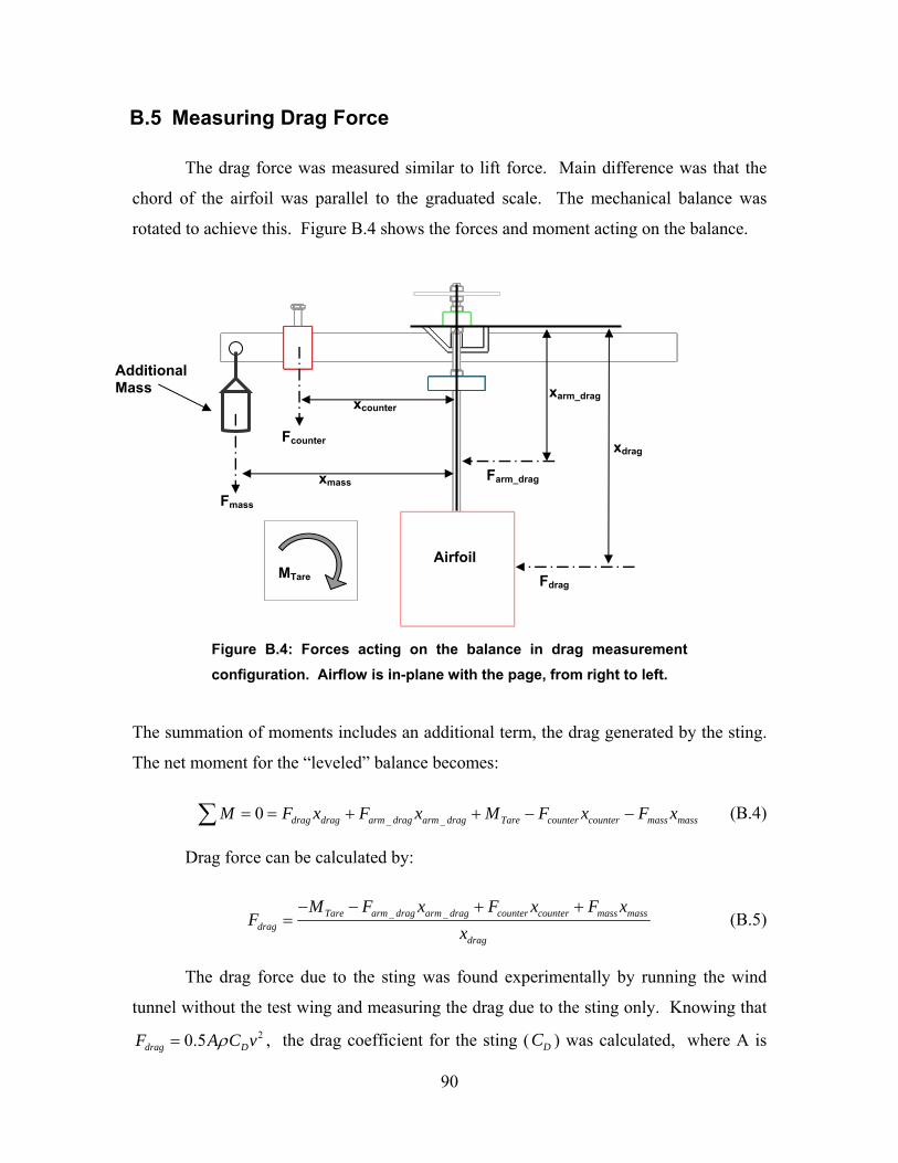
B.5 Measuring Drag Force

The drag force was measured similar to lift force. Main difference was that the

chord of the airfoil was parallel to the graduated scale. The mechanical balance was

rotated to achieve this. Figure B.4 shows the forces and moment acting on the balance.

Figure B.4: Forces acting on the balance in drag measurement configuration. Airflow is in-plane with the page, from right to left.

The summation of moments includes an additional term, the drag generated by the sting.

The net moment for the “leveled” balance becomes:

_ _0 drag drag arm drag arm drag Tare counter counter mass massM F x F x M F x F x= = + + − −∑ (B.4)

Drag force can be calculated by:

_ _Tare arm drag arm drag counter counter mass massdrag

drag

M F x F x F xF

x− − + +

= (B.5)

The drag force due to the sting was found experimentally by running the wind

tunnel without the test wing and measuring the drag due to the sting only. Knowing that

, the drag coefficient for the sting (20.5drag DF A Cρ= v DC ) was calculated, where A is

Farm_drag

xarm_dragxcounter

xmass

xdrag

Additional Mass

Fcounter

Fmass

MTare

AirfoilFdrag

90

the area of the sting perpendicular to the flow, ρ is the air density, and is the air

velocity.

v

B.6 Balance Data Analysis

Measurements of counter-mass position and amount of additional mass were

recorded for each test. Tare moment was calculated for each angle of attack setting. The

measurement data were recorded in Microsoft Excel where the forces and coefficients

were calculated.

91

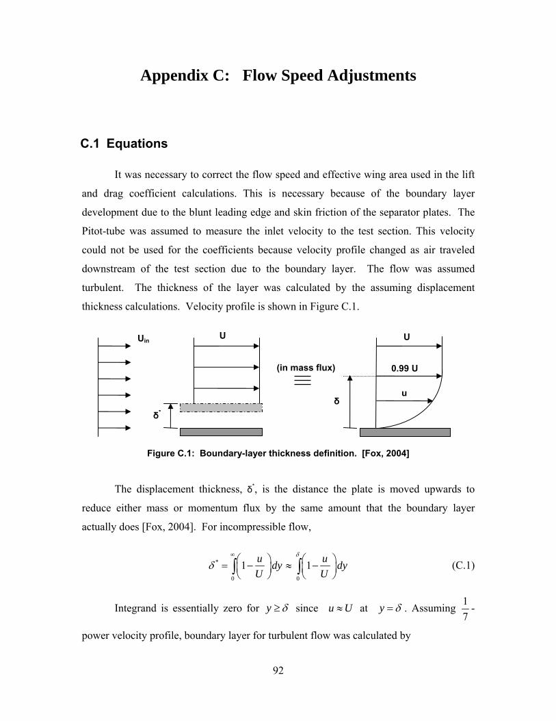
Appendix C: Flow Speed Adjustments

C.1 Equations

It was necessary to correct the flow speed and effective wing area used in the lift

and drag coefficient calculations. This is necessary because of the boundary layer

development due to the blunt leading edge and skin friction of the separator plates. The

Pitot-tube was assumed to measure the inlet velocity to the test section. This velocity

could not be used for the coefficients because velocity profile changed as air traveled

downstream of the test section due to the boundary layer. The flow was assumed

turbulent. The thickness of the layer was calculated by the assuming displacement

thickness calculations. Velocity profile is shown in Figure C.1.

Figure C.1: Boundary-layer thickness definition. [Fox, 2004]

The displacement thickness, δ*, is the distance the plate is moved upwards to

reduce either mass or momentum flux by the same amount that the boundary layer

actually does [Fox, 2004]. For incompressible flow,

*

0 0

1 1u udy dyU

δ

δ∞ ⎛ ⎞ ⎛ ⎞= − ≈ −⎜ ⎟ ⎜ ⎟⎝ ⎠ ⎝ ⎠∫ ∫ U

(C.1)

Integrand is essentially zero for y δ≥ since u U≈ at y δ= . Assuming 17

-

power velocity profile, boundary layer for turbulent flow was calculated by

Uin UU

(in mass flux)

u

0.99 U

δδ*

92

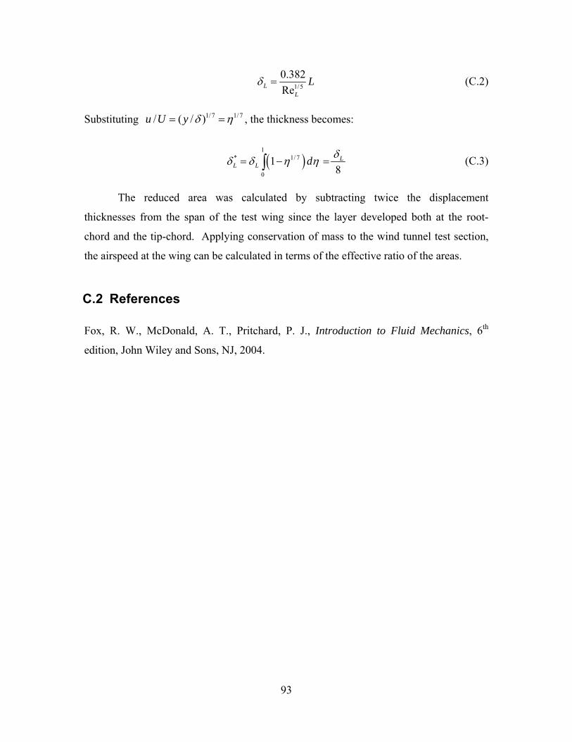
1/5

0.382ReL

L

Lδ = (C.2)

Substituting 1/ 7 1/ 7/ ( / )u U y δ η= = , the thickness becomes:

( )1

* 1/ 7

0

18

LL L d δδ δ η η= − =∫ (C.3)

The reduced area was calculated by subtracting twice the displacement

thicknesses from the span of the test wing since the layer developed both at the root-

chord and the tip-chord. Applying conservation of mass to the wind tunnel test section,

the airspeed at the wing can be calculated in terms of the effective ratio of the areas.

C.2 References

Fox, R. W., McDonald, A. T., Pritchard, P. J., Introduction to Fluid Mechanics, 6th

edition, John Wiley and Sons, NJ, 2004.

93

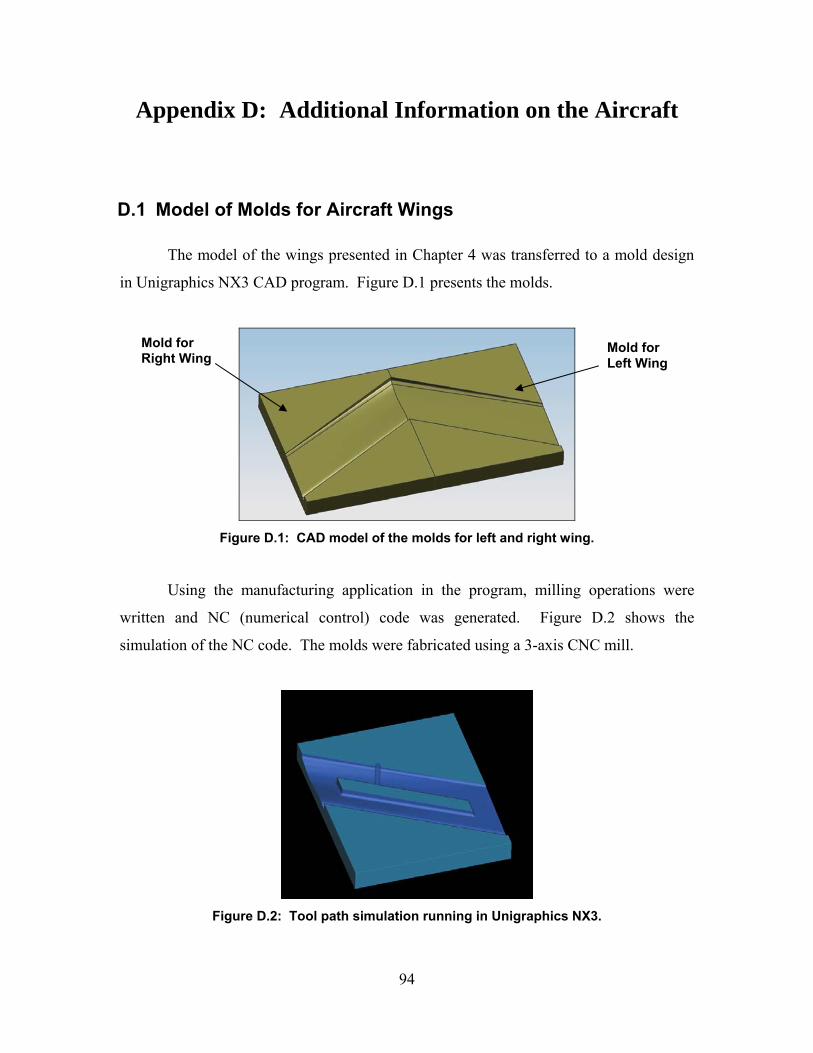
Appendix D: Additional Information on the Aircraft

D.1 Model of Molds for Aircraft Wings

The model of the wings presented in Chapter 4 was transferred to a mold design

in Unigraphics NX3 CAD program. Figure D.1 presents the molds.

Figure D.1: CAD model of the molds for left and right wing.

Using the manufacturing application in the program, milling operations were

written and NC (numerical control) code was generated. Figure D.2 shows the

simulation of the NC code. The molds were fabricated using a 3-axis CNC mill.

Figure D.2: Tool path simulation running in Unigraphics NX3.

Mold for Right Wing

Mold for Left Wing

94

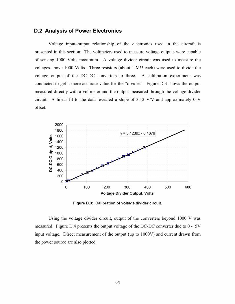
D.2 Analysis of Power Electronics

Voltage input–output relationship of the electronics used in the aircraft is

presented in this section. The voltmeters used to measure voltage outputs were capable

of sensing 1000 Volts maximum. A voltage divider circuit was used to measure the

voltages above 1000 Volts. Three resistors (about 1 MΩ each) were used to divide the

voltage output of the DC-DC converters to three. A calibration experiment was

conducted to get a more accurate value for the “divider.” Figure D.3 shows the output

measured directly with a voltmeter and the output measured through the voltage divider

circuit. A linear fit to the data revealed a slope of 3.12 V/V and approximately 0 V

offset.

y = 3.1239x - 0.1676

0200400600800

100012001400160018002000

0 100 200 300 400 500 600Voltage Divider Output, Volts

DC

-DC

Out

put,

Volts

Figure D.3: Calibration of voltage divider circuit.

Using the voltage divider circuit, output of the converters beyond 1000 V was

measured. Figure D.4 presents the output voltage of the DC-DC converter due to 0 - 5V

input voltage. Direct measurement of the output (up to 1000V) and current drawn from

the power source are also plotted.

95

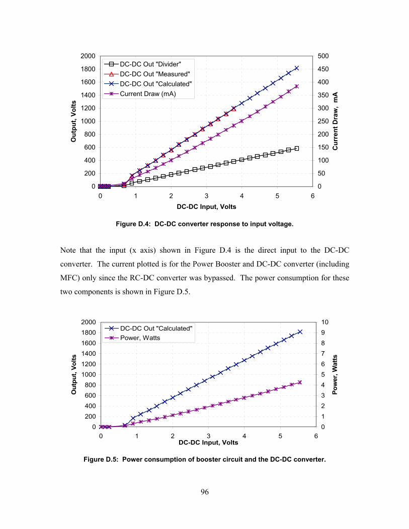
0

200

400

600

800

1000

1200

1400

1600

1800

2000

0 1 2 3 4 5 6DC-DC Input, Volts

Out

put,

Volts

0

50

100

150

200

250

300

350

400

450

500

Cur

rent

Dra

w,

mA

DC-DC Out "Divider"DC-DC Out "Measured"DC-DC Out "Calculated"Current Draw (mA)

Figure D.4: DC-DC converter response to input voltage.

Note that the input (x axis) shown in Figure D.4 is the direct input to the DC-DC

converter. The current plotted is for the Power Booster and DC-DC converter (including

MFC) only since the RC-DC converter was bypassed. The power consumption for these

two components is shown in Figure D.5.

0200400600800

100012001400160018002000

0 1 2 3 4 5 6DC-DC Input, Volts

Out

put,

Volts

012345678910

Pow

er, W

atts

DC-DC Out "Calculated"Power, Watts

Figure D.5: Power consumption of booster circuit and the DC-DC converter.

96

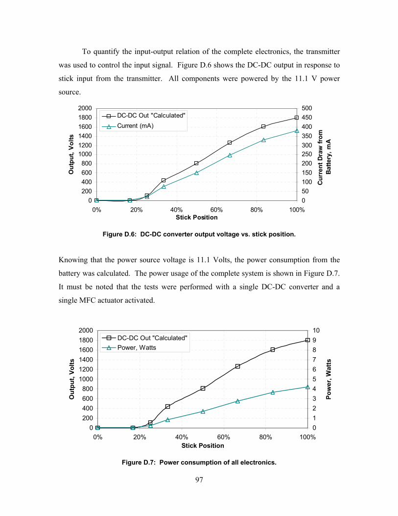
To quantify the input-output relation of the complete electronics, the transmitter

was used to control the input signal. Figure D.6 shows the DC-DC output in response to

stick input from the transmitter. All components were powered by the 11.1 V power

source.

0200400600800

100012001400160018002000

0% 20% 40% 60% 80% 100%Stick Position

Out

put,

Volts

050100150200250300350400450500

Cur

rent

Dra

w fr

om

Batte

ry, m

A

DC-DC Out "Calculated"Current (mA)

Figure D.6: DC-DC converter output voltage vs. stick position.

Knowing that the power source voltage is 11.1 Volts, the power consumption from the

battery was calculated. The power usage of the complete system is shown in Figure D.7.

It must be noted that the tests were performed with a single DC-DC converter and a

single MFC actuator activated.

0200400600800

100012001400160018002000

0% 20% 40% 60% 80% 100%Stick Position

Out

put,

Volts

012345678910

Pow

er, W

atts

DC-DC Out "Calculated"Power, Watts

Figure D.7: Power consumption of all electronics.

97

Looking at the power consumption at 1500 V actuation (77%), approximately 3.4

Watts was measured. The power calculated includes contributions from all onboard

electronics except the motor, which are: The receiver, RC-DC, Booster, DC-DC and the

MFC actuator.

98

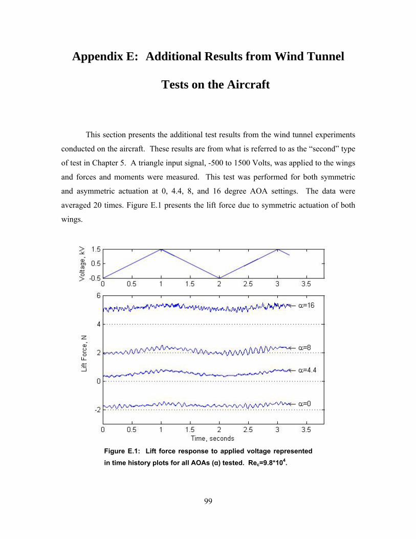
Appendix E: Additional Results from Wind Tunnel

Tests on the Aircraft

This section presents the additional test results from the wind tunnel experiments

conducted on the aircraft. These results are from what is referred to as the “second” type

of test in Chapter 5. A triangle input signal, -500 to 1500 Volts, was applied to the wings

and forces and moments were measured. This test was performed for both symmetric

and asymmetric actuation at 0, 4.4, 8, and 16 degree AOA settings. The data were

averaged 20 times. Figure E.1 presents the lift force due to symmetric actuation of both

wings.

Figure E.1: Lift force response to applied voltage represented in time history plots for all AOAs (α) tested. Rec=9.8*104.

99

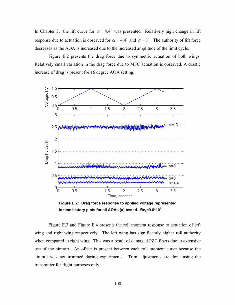
In Chapter 5, the lift curve for was presented. Relatively high change in lift

response due to actuation is observed for and

4.4α =

4.4α = 8α = . The authority of lift force

decreases as the AOA is increased due to the increased amplitude of the limit cycle.

Figure E.2 presents the drag force due to symmetric actuation of both wings.

Relatively small variation in the drag force due to MFC actuation is observed. A drastic

increase of drag is present for 16 degree AOA setting.

Figure E.2: Drag force response to applied voltage represented in time history plots for all AOAs (α) tested. Rec=9.8*104.

Figure E.3 and Figure E.4 presents the roll moment response to actuation of left

wing and right wing respectively. The left wing has significantly higher roll authority

when compared to right wing. This was a result of damaged PZT fibers due to extensive

use of the aircraft. An offset is present between each roll moment curve because the

aircraft was not trimmed during experiments. Trim adjustments are done using the

transmitter for flight purposes only.

100

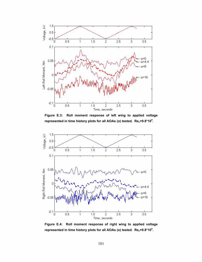
Figure E.3: Roll moment response of left wing to applied voltage represented in time history plots for all AOAs (α) tested. Rec=9.8*104.

Figure E.4: Roll moment response of right wing to applied voltage represented in time history plots for all AOAs (α) tested. Rec=9.8*104.

101

Vita

Onur Bilgen

Onur Bilgen was born on July 9, 1983 in Ankara, Turkey. After elementary

education in Erzurum, a city in north-east Turkey, Onur moved back to Ankara to attend

middle and high school at the Ted Ankara Koleji. During his senior year, Onur spent a

year in Omaha, NE as an exchange student. That year, he applied for, and was accepted

at the George Washington University in Washington, DC. Onur transferred to Virginia

Polytechnic and State University at the end of his freshman year. Onur participated in the

Formula Team, his senior design project, where he led the Drive Train Team and

participated in the 2005 Formula SAE competition in Pontiac, MI. After successfully

competing at the competition, he received his Bachelor of Science degree in Mechanical

Engineering in Honors magna cum laude as a Commonwealth Scholar. Upon graduation,

Onur started his studies towards Master of Science degree. Onur defended his Master of

Science degree on May 10, 2007. He will be studying the use of smart materials for

control of hovering unmanned aircraft for his Doctor of Philosophy degree in Mechanical

Engineering under the direction of Dr. Daniel J. Inman.

102

Documents

Macro Fiber Composite Actuated Unmanned Air Vehicles: Design, … · 2020-01-22 · Macro Fiber Composite Actuated Unmanned Air Vehicles: Design, Development, and Testing Onur Bilgen