Embed Size (px)
Citation preview

glove box guideIrrigation

MACKILLOP FARM MANAGEMENT GROUP
Krysteen McElroy (Chief Executive Officer)Ph: 0408 655 [email protected] www.mackillopgroup.com.au
NATURAL RESOURCES SOUTH EAST
11 Helen Street, Mt Gambier SA 5290Ph: 08 8735 1177 www.naturalresources.sa.gov.au/southeast
PRIMARY INDUSTRIES AND REGIONS SOUTH AUSTRALIA
Level 14 25 Grenfell Street Adelaide, South Australia 5000Ph: +61 8 8226 0995 www.pir.sa.gov.au
This project is jointly funded through Natural Resources South East, Primary Industries and Regions SA and the Australian Government’s National Landcare Programme.
Acknowledgments
CONTRIBUTORS The following have provided information and content for this guide: Adrian Harvey, Rob Palamountain, Michael Zerk, James Heffernan, Daniel Newson, Tim Powell
Photos supplied by Lucerne Australia
Published May 2016
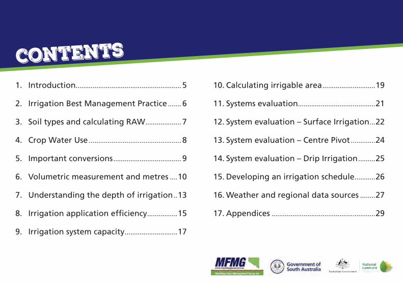
1. Introduction........................................................ 5
2. Irrigation Best Management Practice ....... 6
3. Soil types and calculating RAW ................... 7
4. Crop Water Use ................................................. 8
5. Important conversions .................................... 9
6. Volumetric measurement and metres ....10
7. Understanding the depth of irrigation ..13
8. Irrigation application efficiency ................15
9. Irrigation system capacity ............................17
10. Calculating irrigable area ............................19
11. Systems evaluation .........................................21
12. System evaluation – Surface Irrigation ...22
13. System evaluation – Centre Pivot .............24
14. System evaluation – Drip Irrigation .........25
15. Developing an irrigation schedule ...........26
16. Weather and regional data sources ........27
17. Appendices .......................................................29
contents

DUL – Daily Upper Limit
DLL – Daily Lower Limit
RAW – Readily Available Water
CWU – Crop Water Use
PUR – Pump Utilisation Ratio
Ea- Application Efficiency
NIR – Net Irrigation Requirement
ETO – Reference Crop Evapotranspiration
KC- Crop Coefficient
ETC - Crop Evapotranspiration
acronyms

5
This booklet has been developed as a quick reference guide for irrigators in the South East of SA. As such, a working knowledge of some of the equations and how to apply them is required.
The information provided is adapted from regional irrigation workshops that have been run in conjunction with Mackillop Farm Management Group, Natural Resources South East and Primary Industries and Regions South Australia.
More detailed information can be found on each of the topics through the
• Mackillop Farm Management Group website www.mackillopgroup.com.au
• Natural Resources South East website www.naturalresources.sa.gov.au/southeast
• Primary Industries and Regions South Australia website www.pir.sa.gov.au
1. introduction

6
To assist regional irrigators to improve the management of their irrigation enterprises, the South Australian Research and Development Institute has developed a number of non-prescriptive irrigation best management practices (BMP). They are general principles, rather than explanations on exactly how to manage your irrigation, or which tools to use.
BMP 1: Rate irrigation highly within your farm management system. The best irrigators tend to rate irrigation management as a very high (if not No. 1) priority.
BMP 2: Get to know the soils on your property. The variable ability of different soil types to hold plant-available moisture means irrigators should have a good understanding of soil types and distribution, and incorporate this understanding into their irrigation scheduling.
BMP 3: Design and maintain irrigation systems correctly. Irrigation systems should be designed with several considerations in mind; including crop type, soil type, water quality and quantity. Once a correctly designed system is installed and set up, appropriate maintenance is required to ensure the system provides high standard, long term use.
BMP 4: Monitor all aspects of each irrigation event. Having a thorough understanding of how much water was applied and where it went, should be the goal of every irrigator.
BMP 5: Use objective monitoring tools to schedule irrigation. Using tools which actually measure things, such as soil moisture, can take a lot of guesswork out of the development of an irrigation schedule.
BMP 6: Use more than one tool for scheduling irrigation. Use multiple tools to avoid the potential of getting the wrong information from just a single source.
BMP 7: Retain control of your irrigation scheduling. Don’t let your use of automation or external contractors result in a hands-off approach to irrigation.
BMP 8: Remain open to new information. Continue to seek, and use, new information to help improve your irrigation practice.
2. irrigation best management practice
7
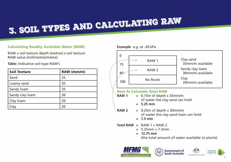
Calculating Readily Available Water (RAW)
RAW = soil texture depth (metres) x soil texture RAW value (millimetres/metre)
Table: Indicative soil-type RAW’s
Soil Texture RAW (mm/m)
Sand 25
Loamy sand 35
Sandy loam 35
Sandy clay loam 30
Clay loam 20
Clay 20
Example e.g. at -20 kPa
How To Calculate Total RAW RAW 1 = 0.15m of depth x 35mm/m of water the clay sand can hold = 5.25 mm
RAW 2 = 0.25m of depth x 30mm/m of water the clay sand loam can hold = 7.5 mm
Total RAW = RAW 1 + RAW 2 = 5.25mm + 7.5mm = 12.75 mm (the total amount of water available to plants)
3. Soil types and calculating RAW
Clay sand 35mm/m available
Sandy clay loam 30mm/m available
Clay 20mm/m available
0
15
40
100
RAW 1
RAW 2
No Roots

8
The ability to assess the amount of water your crop requires is important for seasonal planning and periodic irrigation management (scheduling).
• Apply the correct amount of water for optimum crop development
• Effective use of water within volumetric licence constraints
Things you should know:
1. Crop Water Use (CWU) is expressed in millimetres (mm).
2. How to calculate CWU from Evapotranspiration (ETo) data:
ETo x Kc = ETc Reference Crop Crop Crop Evapotranspiration Coefficient Evapotranspiration
3. How to estimate
Net Irrigation Requirement (NIR) from weather data Note: For crop NIR’s refer to appendix 1
4. Crop Water Use
ETo Kc ETcRainfall (mm)
Net Irrigation
Requirement NIR (mm)
July 42 0.4 17 107
August 59 0.73 43 111
September 81 1.05 85 86
October 119 x 1.05 = 125 - 66 = 59
November 135 1.05 142 58 84
December 171 1.05 180 49 131
January 188 1.05 197 28 169
February 144 1.05 151 30 121
March 137 1.05 144 42 102
April 85 0.95 81 52 29
May 49 0 80
June 37 0 104
TOTALS 1247 1164 813 694
Monthly ETC and Net Irrigation Requirement - Pasture example, Mount Gambier
NOTE: 100mm = 1ML/Ha

9
Water depth & volume
Soil water content, crop water use, rainfall and irrigation all described in depth (mm)
Flow rate and volumes described in Litres (L), Kilolitres (KL), and Megalitres (ML).
1 KL = 1000 L (1m3)
1 ML = 1000 KL
It is important to get conversions correct
Converting depth to Volume
How much water is required to apply 20mm over 37 Ha
Volume (KL) = Target Application (mm) x Ha x 10
= 20 x 37 x 10
= 7400 KL or 7.4 ML
5. Important Conversions

10
Depending on the unit of measure, it can be important to understand the value of each decimal place. The table below explains the value of each decimal place in relation to the unit of measure.
Water meters can measure and display volumes in many different ways.
This may depend on the manufacturer, the type of water meter or often the size of the meter. Some water meters may display the volume as factors of 10 or 100.
The following table provides a definition and details on the units of measure commonly used for irrigation water meters.
6. Volumetric measurement and meters
Unit of Measure First decimal 1.0
Second decimal 0.01
Third decimal 0.001
Kilolitres (KL) 100’s of litres 10’s of litres litres
Megalitres (ML) 100’s of kilolitres 10’s of kilolitres kilolitres
Gigalitres (GL) 100’s of megalitres
10’s of megalitres megalitres
Unit of Measure Description Conversion
Notes on Reading (counting from
left to right)
KL Kilolitre 1 KL = 1000 L 4th digit represents ML
ML Megalitre 1 ML = 1000 KL 1st decimal place represent KL
m3 Cubic metre 1 m3 = 1 KL Same as KL
m3 x 10 Cubic metre times 10 1 m3 x 10 = 10 KL 3rd digit
represents ML
m3 x 100 Cubic metre times 100 1 m3 x 100 = 100 KL 2nd digit
represents ML
Unit Litres Kilolitres Megalitre Gigalitre
1 Litre (L) 1 L 0.001 KL
1 Kilolitre (KL) 1 000 L 1 KL 0.001 ML
1 Megalitre (ML) 1 000 000 L 1 000 KL 1 ML 0.001 GL
1 Gigalitre (GL) 1 000 000 000 L 1 000 000 KL 1 000 ML 1 GL

11
6. Volumetric measurement and meters

12
6. Volumetric measurement and meters

13
The ability to measure and control the depth of irrigation is critical to properly meet the water requirement of your crop, incorporate fertilisers and manage salinity.
• Irrigation system design and specifications • Estimating depth of irrigation from water meter readings
Things you should know:
1. For full cover irrigation, 1 ML/Ha is equivalent to 100 mm irrigation depth (10 KL/Ha = 1 mm) 2. Original Equipment (OE) installation and system performance specifications 3. How to estimate depth of irrigation from meter readings (assumes uniform distribution):
Note: Method 2 is more suited to calculating irrigation depth for individual events or sites pumping small volumes .i.e. drip irrigation.
Example: Start meter reading – 554734, End meter reading – 556882, Irrigated Area – 28ha
7. Understanding the depth of irrigation
Irrigation Rate (ML/ha) =Volume pumped (ML)
Area Irrigated (ha)
Irrigation depth (mm)(Method 1)
=Volume pumped (ML) x 100
Area Irrigated (ha)
Irrigation depth (mm)(Method 2)
=Volume pumped (ML)
(Area Irrigated (ha)) x 10
Irrigation depth (mm) =End reading – Start reading
(Area Irrigated (ha)) x 10
Irrigation depth (mm)
=556882 - 554734
= 7.7mm28 x 10
14
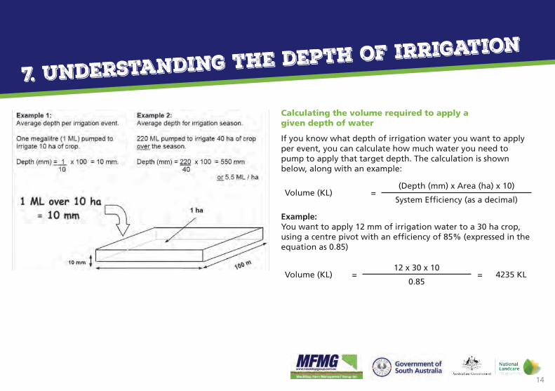
Calculating the volume required to apply a given depth of water
If you know what depth of irrigation water you want to apply per event, you can calculate how much water you need to pump to apply that target depth. The calculation is shown below, along with an example:
Example: You want to apply 12 mm of irrigation water to a 30 ha crop, using a centre pivot with an efficiency of 85% (expressed in the equation as 0.85)
7. Understanding the depth of irrigation
Volume (KL) =12 x 30 x 10
= 4235 KL0.85
Volume (KL) =(Depth (mm) x Area (ha) x 10)
System Efficiency (as a decimal)

15
All systems have losses due to friction, pipe size, maintenance and distance over which the water has to travel. These are usually available from the system designer and are expressed as efficiency curves.
Given the Application Efficiency of your system, how much additional water is required to meet NIR?
Guideline Application Efficiencies of major irrigation systems:
• Surface Irrigation 65% • Centre Pivot 85% • Drip 95%
Example: A 24 hectare stand of pasture requires 15mm irrigation. What total volume needs to be applied under different system efficiencies to provide the required depth of irrigation?
Example: Determine the volume of water required to meet the Net Irrigation Requirements (NIR) of 6.94 ML/Ha using nominal irrigation system efficiency.
As application efficiency declines, the volume of water that must be pumped to meet crop requirement increases.
8. Irrigation Application Efficiency
Total Flow Required (ML)
=(Depth (mm) x Area (ha) x 10)
System Efficiency (as a decimal)
Irrigation Efficiency
15mm 85% 75% 65%
Total Flow Required (ML)
3.6 4.24 480 5.54
Irrigation Type
Application Efficiency
(Ea)
Calculation Total Volume Required (ML/Ha)NIR (ML/Ha) ÷ Ea
Centre Pivot 0.85 6.94 ÷ 0.85 8.16
Surface Irrigation 0.65 6.94 ÷ 0.65 10.68

16
Factors that affect irrigation efficiency
• System design - along with maintenance requirements and site conditions are fundamental factors that influence the overall efficiency of irrigation systems.
• Soils - High irrigation efficiencies are generally easier to achieve on heavier and deeper soils, while low efficiencies are more common for sites located on shallow and free draining soils.
• Sprinkler packages - the right sprinkler package that is well maintained can reduce losses to evaporation and improve the distribution uniformity and application efficiency.
• Pump flow rate - high flow rates for flood irrigation systems can reduce the time required to water each bay and hence use less water per irrigation event.
• Irrigation scheduling - applying the right amount at the right time to match crop water requirements and soil moisture holding capacity can result in less deep drainage and improved efficiency.
• Application depth - if the average application depth is greater than the soil moisture holding capacity it will result in excessive deep drainage per irrigation event and therefore contribute to low overall system efficiency.
Factors to improve irrigation efficiency
Irrigation efficiency can be improved by reducing water losses. There are three major areas where improvements can be made:
• Transmission system: channel treatment or lining options can reduce losses in channel systems. Piped systems should be well maintained to avoid significant losses.
• Application system: Good irrigation system design and maintenance is a key ingredient to achieving high irrigation efficiency. Depending on the system type, the options will vary.
• Irrigation management: Applying the right amount of water at the right time minimises deep drainage losses.
8. Irrigation Application Efficiency
17
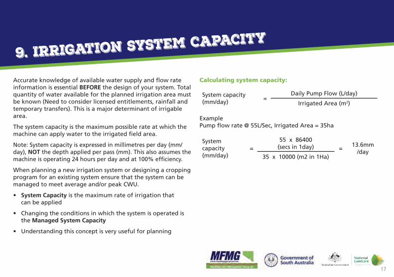
Accurate knowledge of available water supply and flow rate information is essential BEFORE the design of your system. Total quantity of water available for the planned irrigation area must be known (Need to consider licensed entitlements, rainfall and temporary transfers). This is a major determinant of irrigable area.
The system capacity is the maximum possible rate at which the machine can apply water to the irrigated field area.
Note: System capacity is expressed in millimetres per day (mm/day), NOT the depth applied per pass (mm). This also assumes the machine is operating 24 hours per day and at 100% efficiency.
When planning a new irrigation system or designing a cropping program for an existing system ensure that the system can be managed to meet average and/or peak CWU.
• System Capacity is the maximum rate of irrigation that can be applied
• Changing the conditions in which the system is operated is the Managed System Capacity
• Understanding this concept is very useful for planning
Calculating system capacity:
Example Pump flow rate @ 55L/Sec, Irrigated Area = 35ha
9. Irrigation system capacity
System capacity (mm/day)
=Daily Pump Flow (L/day)
Irrigated Area (m2)
System capacity (mm/day)
=55 x 86400
(secs in 1day) =13.6mm
/day35 x 10000 (m2 in 1Ha)
18
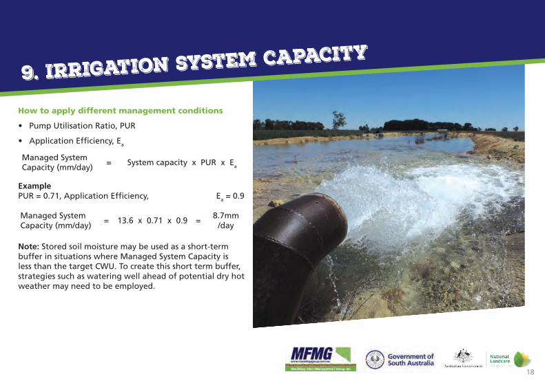
How to apply different management conditions
• Pump Utilisation Ratio, PUR
• Application Efficiency, Ea
Example PUR = 0.71, Application Efficiency, Ea = 0.9
Note: Stored soil moisture may be used as a short-term buffer in situations where Managed System Capacity is less than the target CWU. To create this short term buffer, strategies such as watering well ahead of potential dry hot weather may need to be employed.
9. Irrigation system capacity
Managed System Capacity (mm/day)
= System capacity x PUR x Ea
Managed System Capacity (mm/day)
= 13.6 x 0.71 x 0.9 =8.7mm
/day
19
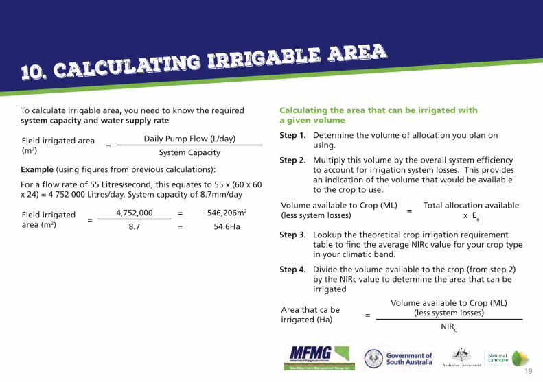
To calculate irrigable area, you need to know the required system capacity and water supply rate
Example (using figures from previous calculations):
For a flow rate of 55 Litres/second, this equates to 55 x (60 x 60 x 24) = 4 752 000 Litres/day, System capacity of 8.7mm/day
Calculating the area that can be irrigated with a given volume
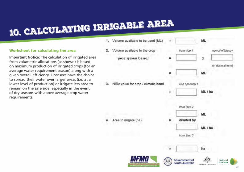
Step 1. Determine the volume of allocation you plan on using.
Step 2. Multiply this volume by the overall system efficiency to account for irrigation system losses. This provides an indication of the volume that would be available to the crop to use.
Step 3. Lookup the theoretical crop irrigation requirement table to find the average NIRc value for your crop type in your climatic band.
Step 4. Divide the volume available to the crop (from step 2) by the NIRc value to determine the area that can be irrigated
10. Calculating irrigable area
Field irrigated area (m2)
=Daily Pump Flow (L/day)
System Capacity
Area that ca be irrigated (Ha)
=Volume available to Crop (ML)
(less system losses)
NIRC
Field irrigated area (m2)
=4,752,000 = 546,206m2
= 54.6Ha8.7
Volume available to Crop (ML)(less system losses)
=Total allocation available
x Ea
20
Worksheet for calculating the area
Important Notice: The calculation of irrigated area from volumetric allocations (as shown) is based on maximum production of irrigated crops (for an average water requirement season) along with a given overall efficiency. Licensees have the choice to spread their water over larger areas (i.e. at a lower level of production) or irrigate less area to remain on the safe side, especially in the event of dry seasons with above average crop water requirements.
10. Calculating irrigable area
21
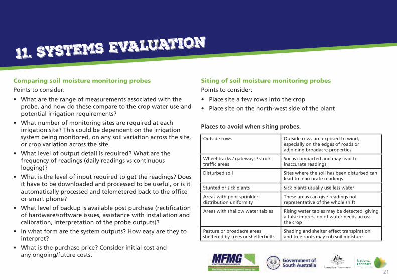
Comparing soil moisture monitoring probes
Points to consider:
• What are the range of measurements associated with the probe, and how do these compare to the crop water use and potential irrigation requirements?
• What number of monitoring sites are required at each irrigation site? This could be dependent on the irrigation system being monitored, on any soil variation across the site, or crop variation across the site.
• What level of output detail is required? What are the frequency of readings (daily readings vs continuous logging)?
• What is the level of input required to get the readings? Does it have to be downloaded and processed to be useful, or is it automatically processed and telemetered back to the office or smart phone?
• What level of backup is available post purchase (rectification of hardware/software issues, assistance with installation and calibration, interpretation of the probe outputs)?
• In what form are the system outputs? How easy are they to interpret?
• What is the purchase price? Consider initial cost and any ongoing/future costs.
Siting of soil moisture monitoring probes
Points to consider:
• Place site a few rows into the crop
• Place site on the north-west side of the plant
Places to avoid when siting probes.
11. Systems Evaluation
Outside rows Outside rows are exposed to wind, especially on the edges of roads or adjoining broadacre properties
Wheel tracks / gateways / stock traffic areas
Soil is compacted and may lead to inaccurate readings
Disturbed soil Sites where the soil has been disturbed can lead to inaccurate readings
Stunted or sick plants Sick plants usually use less water
Areas with poor sprinkler distribution uniformity
These areas can give readings not representative of the whole shift
Areas with shallow water tables Rising water tables may be detected, giving a false impression of water needs across the crop
Pasture or broadacre areas sheltered by trees or shelterbelts
Shading and shelter effect transpiration, and tree roots may rob soil moisture
22
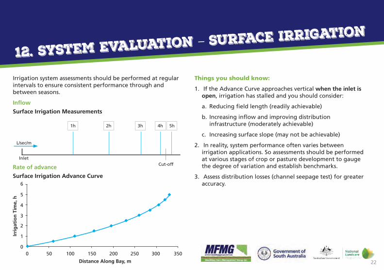
Irrigation system assessments should be performed at regular intervals to ensure consistent performance through and between seasons.
Inflow
Surface Irrigation Measurements
Rate of advance
Surface Irrigation Advance Curve
Things you should know:
1. If the Advance Curve approaches vertical when the inlet is open, irrigation has stalled and you should consider:
a. Reducing field length (readily achievable)
b. Increasing inflow and improving distribution infrastructure (moderately achievable)
c. Increasing surface slope (may not be achievable)
2. In reality, system performance often varies between irrigation applications. So assessments should be performed at various stages of crop or pasture development to gauge the degree of variation and establish benchmarks.
3. Assess distribution losses (channel seepage test) for greater accuracy.
12. System Evaluation – Surface Irrigation
L/sec/m
InletCut-off
1h 2h 3h 4h 5h
6
5
4
3
2
1
00 50 100 150 200
Distance Along Bay, m
Irri
gat
ion
Tim
e, h
250 300 350
23
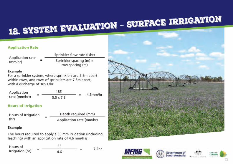
Application Rate
Example For a sprinkler system, where sprinklers are 5.5m apart within rows, and rows of sprinklers are 7.3m apart, with a discharge of 185 L/hr:
Hours of Irrigation
Example
The hours required to apply a 33 mm irrigation (including leaching) with an application rate of 4.6 mm/h is:
12. System Evaluation – Surface Irrigation
Application rate (mm/hr))
=185
= 4.6mm/hr5.5 x 7.3
Hours of Irrigation (hr)
=33
= 7.2hr4.6
Hours of Irrigation (hr)
=Depth required (mm)
Application rate (mm/hr)
Application rate (mm/hr)
=Sprinkler flow rate (L/hr)
Sprinkler spacing (m) × row spacing (m)
24
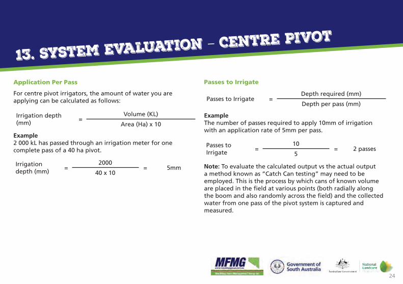
Application Per Pass
For centre pivot irrigators, the amount of water you are applying can be calculated as follows:
Example 2 000 kL has passed through an irrigation meter for one complete pass of a 40 ha pivot.
Passes to Irrigate
Example The number of passes required to apply 10mm of irrigation with an application rate of 5mm per pass.
Note: To evaluate the calculated output vs the actual output a method known as “Catch Can testing” may need to be employed. This is the process by which cans of known volume are placed in the field at various points (both radially along the boom and also randomly across the field) and the collected water from one pass of the pivot system is captured and measured.
13. System Evaluation – Centre Pivot
Irrigation depth (mm)
=2000
= 5mm40 x 10
Passes to Irrigate
=10
= 2 passes5
Irrigation depth (mm)
=Volume (KL)
Area (Ha) x 10
Passes to Irrigate =Depth required (mm)
Depth per pass (mm)
25
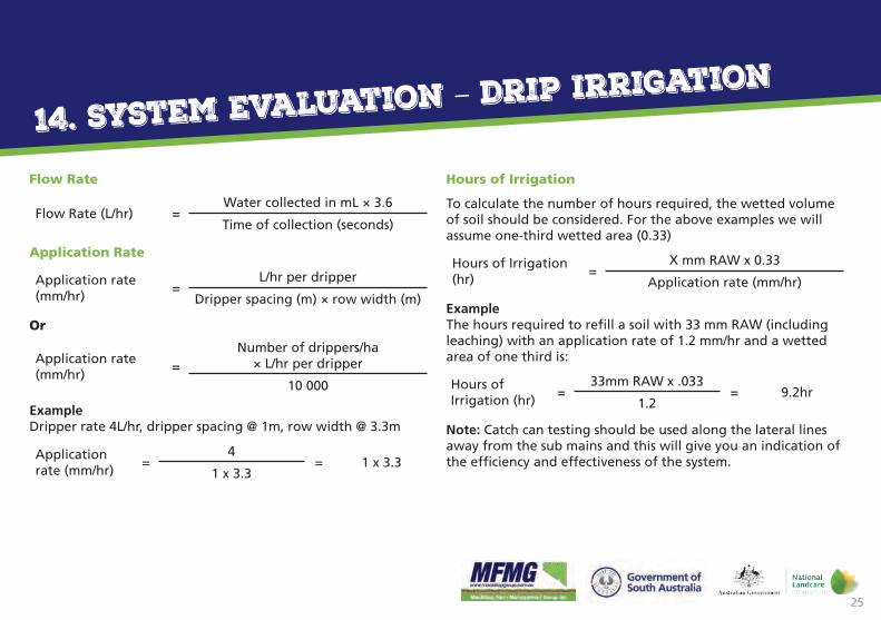
Flow Rate
Application Rate
Or
Example Dripper rate 4L/hr, dripper spacing @ 1m, row width @ 3.3m
Hours of Irrigation
To calculate the number of hours required, the wetted volume of soil should be considered. For the above examples we will assume one-third wetted area (0.33)
Example The hours required to refill a soil with 33 mm RAW (including leaching) with an application rate of 1.2 mm/hr and a wetted area of one third is:
Note: Catch can testing should be used along the lateral lines away from the sub mains and this will give you an indication of the efficiency and effectiveness of the system.
14. System Evaluation – Drip Irrigation
Application rate (mm/hr)
=4
= 1 x 3.31 x 3.3
Hours of Irrigation (hr)
=33mm RAW x .033
= 9.2hr1.2
Flow Rate (L/hr) =Water collected in mL × 3.6
Time of collection (seconds)
Hours of Irrigation (hr)
=X mm RAW x 0.33
Application rate (mm/hr)Application rate (mm/hr)
=L/hr per dripper
Dripper spacing (m) × row width (m)
Application rate (mm/hr)
=Number of drippers/ha
× L/hr per dripper
10 000
26
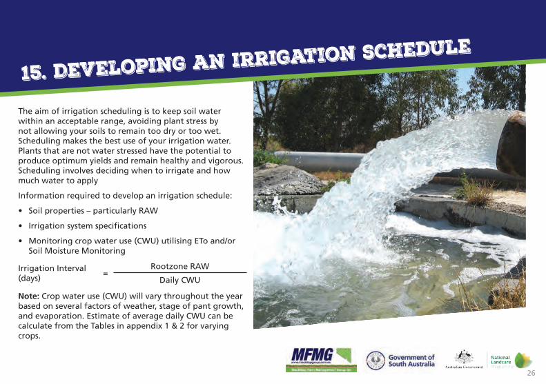
The aim of irrigation scheduling is to keep soil water within an acceptable range, avoiding plant stress by not allowing your soils to remain too dry or too wet. Scheduling makes the best use of your irrigation water. Plants that are not water stressed have the potential to produce optimum yields and remain healthy and vigorous. Scheduling involves deciding when to irrigate and how much water to apply
Information required to develop an irrigation schedule:
• Soil properties – particularly RAW
• Irrigation system specifications
• Monitoring crop water use (CWU) utilising ETo and/or Soil Moisture Monitoring
Note: Crop water use (CWU) will vary throughout the year based on several factors of weather, stage of pant growth, and evaporation. Estimate of average daily CWU can be calculate from the Tables in appendix 1 & 2 for varying crops.
15. Developing an irrigation schedule
Irrigation Interval (days)
=Rootzone RAW
Daily CWU
27
DEWNR/NRM
NatureMaps
NatureMaps, www.naturemaps.sa.gov.au is an initiative of the Department of Environment, Water and Natural Resources that provides a common access point to maps and geographic information about South Australia’s natural resources in an interactive online mapping format.
• Administrative Boundaries
• Cadastral Information
• Coast and Marine
• Fauna and Flora
• Fire
• Heritage and Tourism
• Landscapes
• Protected Areas
• Tenure and Landuse
• Vegetation Mapping
• *NEW* Water (Ground and Surface)
• Wetlands
• Graticules, Grids and Map Tiles
• Photo Centres and Flight Line
nrmWEATHER
To access detailed weather data from the Natural Resources South East automatic weather station (AWS) website, click on se-aws.nrmspace.com.au.
This link takes you to the nrmWEATHER homepage and a map of the South East (with site locations of the 19 regional AWS’s) and a menu with dedicated links to each site.
For detailed site information, click on the menu link for the relevant site of interest. This will take you to a summary page for that station, with a range of archived data links above a table comprising the most recent site information.
The ‘Download’ link allows you to view or save data from within any data range you enter (Note the format required for entering dates in the adjacent brackets). This facility gives you the option of retrieving either daily or 15 minute data.
Saved data can be exported into Excel spreadsheets; allowing you to produce tables and graphs from the information of interest.
16. Weather and regional data sources
28
Bureau of Meteorology
AWS
The Bureau of Meteorology has several Automated Weather Station’s AWS (and one manned site) in the South East. View data from these sites by scrolling down to the ‘Upper South East and Lower South East’ table at
www.bom.gov.au/sa/observations/saall.shtml.
Click on the site link (in the first column) for more detailed information.
Met Eye
MetEye™ — our new interactive weather resource, helps you view real-time weather observations and seven day forecast information. Using your mouse or tapping on your tablet you can now view different weather elements such as real-time temperature, rainfall, radar images, cloud cover and wind speed for one location. It’s a new way to view local weather. When the roll out of the Next Generation Forecast and Warning System is complete, MetEye™ will display forecasts, satellite and radar imagery, as well as the Bureau’s weather
www.bom.gov.au/australia/meteye
PIRSA
AGINSIGHT
The new AgInsight South Australia site is part of the 4 year Agribusiness Accelerator Program and a key part of the Premium food and wine produced in our clean environment and exported to the world economic priority.
AgInsight South Australia has more than 150 geospatial layers that can show you:
• land type
• land zoning
• transport infrastructure
• energy infrastructure
• commodities produced
• climate information
• water availability
• and much more.
www.aginsight.sa.gov.au
16. Weather and regional data sources
29
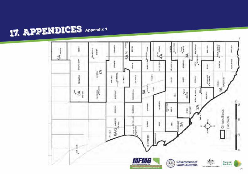
17. Appendices Appendix 1
30
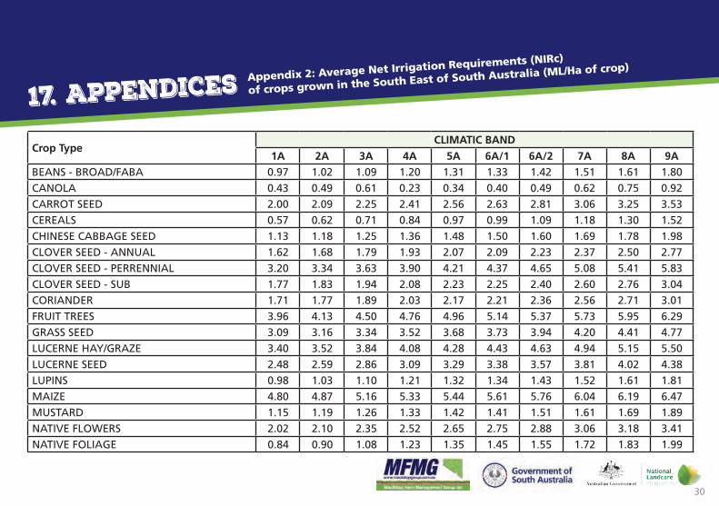
17. Appendices Appendix 2: Average Net Irrigation Requirements (NIRc)
of crops grown in the South East of South Australia (ML/Ha of crop)
Crop TypeCLIMATIC BAND
1A 2A 3A 4A 5A 6A/1 6A/2 7A 8A 9ABEANS - BROAD/FABA 0.97 1.02 1.09 1.20 1.31 1.33 1.42 1.51 1.61 1.80CANOLA 0.43 0.49 0.61 0.23 0.34 0.40 0.49 0.62 0.75 0.92CARROT SEED 2.00 2.09 2.25 2.41 2.56 2.63 2.81 3.06 3.25 3.53CEREALS 0.57 0.62 0.71 0.84 0.97 0.99 1.09 1.18 1.30 1.52CHINESE CABBAGE SEED 1.13 1.18 1.25 1.36 1.48 1.50 1.60 1.69 1.78 1.98CLOVER SEED - ANNUAL 1.62 1.68 1.79 1.93 2.07 2.09 2.23 2.37 2.50 2.77CLOVER SEED - PERRENNIAL 3.20 3.34 3.63 3.90 4.21 4.37 4.65 5.08 5.41 5.83CLOVER SEED - SUB 1.77 1.83 1.94 2.08 2.23 2.25 2.40 2.60 2.76 3.04CORIANDER 1.71 1.77 1.89 2.03 2.17 2.21 2.36 2.56 2.71 3.01FRUIT TREES 3.96 4.13 4.50 4.76 4.96 5.14 5.37 5.73 5.95 6.29GRASS SEED 3.09 3.16 3.34 3.52 3.68 3.73 3.94 4.20 4.41 4.77LUCERNE HAY/GRAZE 3.40 3.52 3.84 4.08 4.28 4.43 4.63 4.94 5.15 5.50LUCERNE SEED 2.48 2.59 2.86 3.09 3.29 3.38 3.57 3.81 4.02 4.38LUPINS 0.98 1.03 1.10 1.21 1.32 1.34 1.43 1.52 1.61 1.81MAIZE 4.80 4.87 5.16 5.33 5.44 5.61 5.76 6.04 6.19 6.47MUSTARD 1.15 1.19 1.26 1.33 1.42 1.41 1.51 1.61 1.69 1.89NATIVE FLOWERS 2.02 2.10 2.35 2.52 2.65 2.75 2.88 3.06 3.18 3.41NATIVE FOLIAGE 0.84 0.90 1.08 1.23 1.35 1.45 1.55 1.72 1.83 1.99
31
17. Appendices
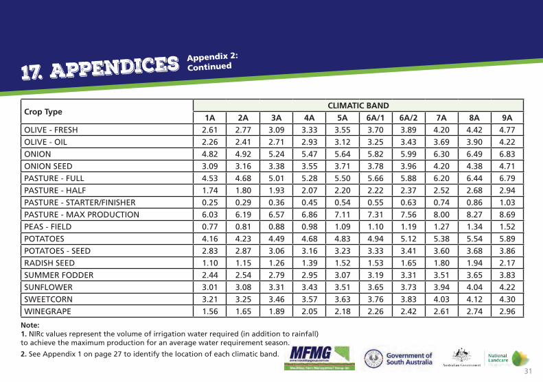
Note: 1. NIRc values represent the volume of irrigation water required (in addition to rainfall) to achieve the maximum production for an average water requirement season.
2. See Appendix 1 on page 27 to identify the location of each climatic band.
Appendix 2:
Continued
Crop TypeCLIMATIC BAND
1A 2A 3A 4A 5A 6A/1 6A/2 7A 8A 9AOLIVE - FRESH 2.61 2.77 3.09 3.33 3.55 3.70 3.89 4.20 4.42 4.77OLIVE - OIL 2.26 2.41 2.71 2.93 3.12 3.25 3.43 3.69 3.90 4.22ONION 4.82 4.92 5.24 5.47 5.64 5.82 5.99 6.30 6.49 6.83ONION SEED 3.09 3.16 3.38 3.55 3.71 3.78 3.96 4.20 4.38 4.71PASTURE - FULL 4.53 4.68 5.01 5.28 5.50 5.66 5.88 6.20 6.44 6.79PASTURE - HALF 1.74 1.80 1.93 2.07 2.20 2.22 2.37 2.52 2.68 2.94PASTURE - STARTER/FINISHER 0.25 0.29 0.36 0.45 0.54 0.55 0.63 0.74 0.86 1.03PASTURE - MAX PRODUCTION 6.03 6.19 6.57 6.86 7.11 7.31 7.56 8.00 8.27 8.69PEAS - FIELD 0.77 0.81 0.88 0.98 1.09 1.10 1.19 1.27 1.34 1.52POTATOES 4.16 4.23 4.49 4.68 4.83 4.94 5.12 5.38 5.54 5.89POTATOES - SEED 2.83 2.87 3.06 3.16 3.23 3.33 3.41 3.60 3.68 3.86RADISH SEED 1.10 1.15 1.26 1.39 1.52 1.53 1.65 1.80 1.94 2.17SUMMER FODDER 2.44 2.54 2.79 2.95 3.07 3.19 3.31 3.51 3.65 3.83SUNFLOWER 3.01 3.08 3.31 3.43 3.51 3.65 3.73 3.94 4.04 4.22SWEETCORN 3.21 3.25 3.46 3.57 3.63 3.76 3.83 4.03 4.12 4.30WINEGRAPE 1.56 1.65 1.89 2.05 2.18 2.26 2.42 2.61 2.74 2.96
32
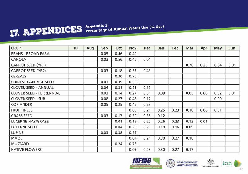
17. Appendices Appendix 3:
Percentage of Annual Water Use (% Use)
CROP Jul Aug Sep Oct Nov Dec Jan Feb Mar Apr May Jun
BEANS - BROAD FABA 0.05 0.46 0.49
CANOLA 0.03 0.56 0.40 0.01
CARROT SEED (YR1) 0.70 0.25 0.04 0.01
CARROT SEED (YR2) 0.03 0.18 0.37 0.43
CEREALS 0.30 0.70
CHINESE CABBAGE SEED 0.03 0.39 0.58
CLOVER SEED - ANNUAL 0.04 0.31 0.51 0.15
CLOVER SEED - PERRENNIAL 0.03 0.14 0.27 0.31 0.09 0.05 0.08 0.02 0.01
CLOVER SEED - SUB 0.08 0.27 0.48 0.17 0.00
CORIANDER 0.05 0.25 0.46 0.23
FRUIT TREES 0.06 0.21 0.25 0.23 0.18 0.06 0.01
GRASS SEED 0.03 0.17 0.30 0.38 0.12
LUCERNE HAY/GRAZE 0.01 0.15 0.22 0.26 0.23 0.12 0.01
LUCERNE SEED 0.04 0.25 0.29 0.18 0.16 0.09
LUPINS 0.03 0.38 0.59
MAIZE 0.04 0.21 0.30 0.27 0.18
MUSTARD 0.24 0.76
NATIVE FLOWERS 0.03 0.23 0.30 0.27 0.17

33
17. Appendices Appendix 3:
Continued
CROP Jul Aug Sep Oct Nov Dec Jan Feb Mar Apr May Jun
NATIVE FOLIAGE 0.18 0.42 0.33 0.07
OLIVE - FRESH 0.09 0.21 0.25 0.23 0.17 0.05
OLIVE - OIL 0.07 0.21 0.26 0.24 0.17 0.04
ONION 0.04 0.13 0.20 0.25 0.23 0.15
ONION SEED 0.01 0.07 0.24 0.34 0.33
PASTURE - FULL 0.01 0.07 0.14 0.18 0.21 0.19 0.15 0.05
PASTURE - FINISHER 0.06 0.50 0.44
PASTURE - STARTER 0.15 0.49 0.28 0.07 0.02
PASTURE - MAX PRODUCTION 0.02 0.08 0.14 0.18 0.20 0.18 0.15 0.05
PEAS - FIELD 0.03 0.54 0.43
POTATOES 0.04 0.19 0.28 0.33 0.16
POTATOES - SEED 0.05 0.24 0.37 0.34
RADISH SEED 0.02 0.23 0.51 0.23
SUMMER FODDER 0.00 0.14 0.30 0.27 0.21 0.08
SUNFLOWER 0.01 0.15 0.40 0.37 0.08
SWEETCORN 0.00 0.22 0.43 0.35
WINEGRAPE 0.05 0.33 0.27 0.21 0.13 0.01
Note: The NIRc values used to calculate the percentage of annual water use are based on the irrigated crop achieving maximum production for an average water requirement season and are to be used as a guide only.