Embed Size (px)
Citation preview

M
Machine Recognition of Objects
Tomaso Poggio and Shimon UllmanDepartment of Brain and Cognitive Sciences,McGovern Institute, Massachusetts Institute ofTechnology, Cambridge, MA, USA
Related Concepts
�Object Class Recognition (Categorization); �VisualCortex Models for Object Recognition
Definition
Machine recognition of objects is the task of locatingand recognizing a given object in an image and con-sists of the following steps: object detection, featureextraction, and recognition.
Background
Early computer vision recognition schemes focusedprimarily on the recognition of rigid three-dimensional(3D) objects, such as machine parts, tools, and cars.This is a challenging problem because the same objectcan have markedly different appearances when viewedfrom different directions. It proved possible to dealsuccessfully with this difficulty by using detailed 3Dmodels of the viewed objects, which were comparedwith the projected 2D image (e.g., [14, 18, 33]). Overthe last decade or so, computational models have madesignificant progress in the task of recognizing natural
object categories under realistic, relatively uncon-strained viewing conditions. Within object recognition,it is common to distinguish two main tasks: identifica-tion, for instance, recognizing a specific face amongother faces, and categorization, for example, recogniz-ing a car among other object classes. We will discussboth of these tasks below and use “recognition” toinclude both.
The qualitative improvement in the performance ofrecognition models can be attributed to three maincomponents. The first is the use of extensive learningin constructing recognition models. In this framework,rather than specifying a particular model, the schemestarts with a large family of possible models anduses observed examples to guide the construction ofa specific model which is best suited to the observeddata. The second component was the development ofnew forms of object representation for the purposeof categorization, based on both computational con-siderations and guidelines from known properties ofthe visual cortex. These two components, representa-tion and learning, are interrelated: initially, the classrepresentation provides a family of plausible models,and effective learning methods are then used to con-struct a particular model for a novel class such as“dog” or “airplane” based on observed examples. Thethird component was the use of new statistical learn-ing techniques, such as regularization classifiers (SVMand others) and Bayesian inference (such as graphi-cal models). We next discuss each of these advancesin more detail.
Learning instead of design. A conceptual advancethat facilitated recent progress in object recognitionwas the idea of learning the solution to a specific
K. Ikeuchi (ed.), Computer Vision, DOI 10.1007/978-0-387-31439-6,© Springer Science+Business Media New York 2014

M 470 Machine Recognition of Objects
classification problem from examples, rather thanfocusing on the classifier design. This was a markeddeparture from the dominant practices at the time:instead of an expert program with a predetermined setof logical rules, the appropriate model was learnedand selected from a possibly infinite set of models,based on a set of examples. The techniques used inthe 1990s originated in the area of supervised learning,where image examples are provided together with theappropriate class labels (e.g., “face” or “non-face”). Acomprehensive theory of the foundations of supervisedlearning has been developed, with roots in functionalanalysis and probability theory [6, 26, 27, 36]. Theformal analysis of learning continues to evolve and tocontribute to our understanding of the role of learningin visual recognition.
New image representations. A recognition schemetypically extracts during learning a set of measure-ments or “features” and uses them to construct newobject representations. Objects are then classified andrecognized based on their feature representation. Fea-ture selection and object representation are crucial,because they facilitate the identification of elementsthat are shared by objects in the same class and sup-port discrimination between similar objects and cat-egories. Different types of visual features have beenused in computational models in the past, ranging fromsimple local-image patterns such as wavelets, edges,blobs, or local-edge combinations to abstract three-dimensional shape primitives, such as cylinders [21],spheres, cubes, and the like [4].
A common aspect of most past recognition schemesis that they use a fixed small generic set of featuretypes to represent all objects and classes. In con-trast, recent recognition schemes use pictorial featuresextracted from examples, such as object fragmentsor patches, together with their spatial arrangement[1, 3, 19, 30]. Unlike generic parts, these schemes usea large set of features, extracted from different classesof objects. The use of large feature sets is also con-nected to an interesting new trend in signal processing,related to “over-complete” representations. Instead ofrepresenting a signal in terms of a traditional completerepresentation, such as Fourier components, one usesa redundant basis (such as the combination of severalcomplete bases).
Representations using such features have been usedsuccessfully in recent computer vision recognition
systems for two reasons. First, these representationscan be learned and used efficiently; second, theyproved to capture effectively the broad range of vari-ability in appearance within a visual class.
An additional comment is appropriate. The repre-sentations described above are view based, as opposedto object-centered models. A representation based onimage appearance can include not only 2D image prop-erties but also 3D aspects such as local depth variationsor 3D curvature.
New statistical learning methods. Over the last fewyears, the mathematics of learning has become the“lingua franca” of large areas of computer science and,in particular, of computer vision. As we discussed,the use of a learning framework enabled a qualita-tive jump in object recognition. Whereas the initialtechniques used to construct useful classification mod-els from data were quite simple, there are now moreefficient algorithms originally introduced in the areaof learning in the 1990s such as regularization algo-rithms (also called kernel machines), which includeSVM [35, 36] and boosting [12]. By now, the areaof learning has grown to include, in addition to dis-criminative algorithms, probabilistic approaches withthe goal of providing full probability distributions assolutions to object recognition tasks. These techniquesare mostly Bayesian and range from graphical mod-els [13, 15] to hierarchical Bayesian models [16, 17].At the same time, the focus of research is shiftingfrom supervised to unsupervised and semisupervisedlearning problems, using techniques such as manifoldlearning [2]. Semisupervised problems, in which thetraining set consists of a large number of unlabeledexamples and a small number of labeled ones, aregaining attention.
Application
A number of early schemes, mainly focusing on theclass of human faces, obtained significant improve-ment over previous methods [5, 29, 31, 32, 38].The techniques have evolved to reach practicalapplications, as evidenced by their use in currentdigital cameras. The more recent versions of thesecomputational schemes have started to deal success-fully with an increasing range of complex object

Machine Recognition of Objects 471 M
M
categories such as pedestrians, cars, motorcycles, air-planes, horses, and the like, in unconstrained naturalscenes, to deal with a broad range of objects withineach class (e.g., [1, 8, 19, 22–24, 30, 34, 39]). The algo-rithms that were refined over the last few years can dealsuccessfully with a large number of different objectclasses, in complex and highly cluttered scenes. Theyare being applied to databases of hundreds [9] and eventhousands of object classes [7]. Yearly competitions incomputer-based recognition, such as the Pascal chal-lenge [25, 28], witness continuous improvement in therange of classes and in scene complexity successfullyhandled by automatic object categorization algorithms[10, 11, 37].
References
1. Agarwal S, Roth D (2002) Learning a sparse representationfor object recognition. In: Proceedings of the 7th ECCV,Copenhagen, pp 113–130
2. Belkin M, Niyogi P (2004) Semi-supervised learning onRiemannian manifolds. Mach Learn J 56:209–239
3. Belongie S, Malik J, Puzicha J (2002) Shape matchingand object recognition using shape contexts. IEEE PAMI24(4):509–522
4. Biederman I (1985) Human image understanding: recentresearch and a theory. Comput Vis Graph Image Process32:29–73
5. Brunelli R, Poggio T (1993) Face recognition: fea-tures versus templates. IEEE Trans PAMI 15(10):1042–1052
6. Cucker F, Smale S (2002) On the mathematical foundationsof learning. Bull Am Math Soc 39:1–50
7. Deng J, Dong W, Socher R, Li LJ, Li K, Fei-Fei L (2009)ImageNet: a large-scale hierarchical image database. In:IEEE computer vision and pattern recognition (CVPR),Miami
8. Fei-Fei L, Fergus R, Perona P (2003) A Bayesian approachto unsupervised one-shot learning of object categories. In:Proceedings of the ICCV, Wisconsin
9. Fei-Fei L, Fergus R, Perona P (2004) Learning generativevisual models from few training examples: an incremen-tal Bayesian approach tested on 101 object categories. In:IEEE conference on computer vision pattern recognition(CVPR 2004), workshop on generative-model based vision,Washington, DC
10. Felzenszwalb D, McAllester D, Ramanan A (2008) Dis-criminatively trained, multiscale, deformable part model. In:Proceedings of the IEEE conference on computer visionpattern recognition (CVPR), Anchorage
11. Felzenszwalb PF, Girshick RB, McAllester D, RamananD (2009) Object detection with discriminatively trainedpart based models. IEEE Trans Pattern Anal Mach Intell32:1627–1645
12. Freund Y, Schapire RE (1997) A decision-theoretic gener-alization of on-line learning and an application to boosting.J Comput Syst Sci 55(1):119–139
13. Geman S (2005) On the formulation of a compositionmachine. Technical report, Division of Applied Mathemat-ics, Brown University
14. Grimson WEL (1990) Object recognition by computer. MIT,Cambridge
15. Jordan I (2004) Graphical models. Stat Sci (Special issue onBayesian Stat) 19:140–155
16. Kemp C, Tenenbaum JB (2008) The discovery of structuralform. Proc Natl Acad Sci 105(31):10687–10692
17. Lee TS, Mumford D (2003) Hierarchical Bayesian inferencein the visual cortex. J Opt Soc Am A Opt Image Sci Vis20(7):1434–1448.
18. Lowe DG (1987) Three-dimensional object recognitionfrom single two-dimensional images. J Artif Intell 31:355–395
19. Lowe D (2004) Distinctive image features fromscale-invariant key-points. Int J Comput Vis 60(2):91–110
20. Marr D (1982) Vision: a computational investigationinto the human representation and visual information.W.H. Freeman, New York
21. Marr D, Nishihara HK (1978) Representation and recogni-tion of the spatial organisation of three-dimensional shapes.Proc R Soc Lond B 200:269–294
22. Mohan A, Papageorgiou C, Poggio T (2001) Example-basedobject detection in images by components. IEEE TransPattern Anal Mach Intell 23:349–361
23. Papageorgiou C, Evgeniou T, Mukherjee S, Poggio T (1998)A trainable pedestrian detection system. In: IEEE interna-tional conference on intelligent vehicles, Stuttgart, vol 1,pp 241–246
24. Papageorgiou C, Oren M, Poggio T (1998) A generalframework for object detection. In: Proceedings of theinternational conference on computer vision, Bombay, 4–7Jan 1998
25. Pascal website. http://pascallin.ecs.soton.ac.uk/challenges/voc/
26. Poggio T, Smale S (2003) The mathematics of learning:dealing with data. Notices AMS 50:537–544
27. Poggio T, Rifkin R, Mukherjee S, Niyogi P (2004) Gen-eral conditions for predictivity in learning theory. Nature428:419–422
28. Ponce J, Berg TL, Everingham M, Forsyth DA, Hebert M,Lazebnik S, Marszalek M, Schmid C, Russell BC, TorralbaA, Williams CKI, Zhang J, Zisserman A (2007) In: Ponce J,Hebert M, Schmid C, Zisserman A (eds) Toward category-level object recognition. Lecture notes in computer science.Springer, Berlin
29. Rowley H, Baluja S, Kanade T (1998) Neural network-based face detection. IEEE Trans Pattern Anal Mach Intell(PAMI) 20(1):23–38
30. Sali E, Ullman S (1999) Combining class-specific frag-ments for object classification. In: Proceedings of the 10thBritish machine vision conference, Nottingham, vol 1,pp 203–213
31. Sung K, Poggio T (1998) Example-based learning for view-based human face detection. IEEE Trans Pattern Anal MachIntell 20(1):39–51

M 472 Many-to-Many Graph Matching
32. Turk M, Pentland A (1991) Eigen faces for recognition.J Cognit Neurosci 3(1):71–86
33. Ullman S, Basri R (1991) Recognition by linear combina-tion of models. IEEE PAMI 13(10):992–1006
34. Ullman S, Vidal-Naquet M, Sali E (2002) Visual featuresof intermediate complexity and their use in classification.Nature Neurosci 5(7):1–6
35. Vapnik N (1995) The nature of statistical learning theory.Springer, New York
36. Vapnik N (1998) Statistical learning theory. Wiley,New York
37. Vedaldi A, Gulshan V, Varma M, Zisserman A (2009) Mul-tiple Kernels for object detection. In: Proceedings of theinternational conference on computer vision, Kyoto
38. Viola P, Jones M (2001) Robust real-time object detection.Int J Comput Vis 56:151–177
39. Zhang J, Zisserman A (2006) Dataset issues in object recog-nition. In: Ponce J, Hebert M, Schmid C, Zisserman A (eds)Toward category-level object recognition. Springer, Berlin,pp 29–48
Many-to-Many GraphMatching
Fatih Demirci1, Ali Shokoufandeh2 andSven J. Dickinson3
1Department of Computer Engineering, TOBBUniversity of Economics and Technology, Sogutozu,Ankara, Turkey2Department of Computer Science, Drexel University,Philadelphia, PA, USA3Department of Computer Science, University ofToronto, Toronto, ON, Canada
Synonyms
Error-correcting graph matching; Error-tolerant graphmatching; Inexact matching; Transportation problem
Definition
When objects exhibit large within-class variationand/or when image features are under- or over-segmented, the image features extracted from twoexemplars belonging to the same category may nolonger be in one-to-one correspondence but, in gen-eral, many-to-many correspondence. If the features arestructured, i.e., captured in a graph, then computingthe correct correspondence can be formulated as amany-to-many graph matching problem.
Background
The matching of image features to object models istypically formulated as a one-to-one assignment prob-lem, based on the assumption that for every salientimage feature belonging to the object to be matched,e.g., SIFT feature, image patch, contour fragment,there exists a single corresponding feature on themodel (and vice versa). While the one-to-one corre-spondence assumption has been prevalent in the objectrecognition community throughout its entire evolution,including the paradigms of graph matching [9], align-ment [13], geometric invariants [11], local appearance[14], and a recent return to local contour-based fea-tures [8], one-to-one feature correspondence is a highlyrestrictive assumption that breaks down as within-classvariation increases and as the segmentation and extrac-tion of more abstract image features suffer from over-or under-segmentation [7]. In the more general case,feature correspondence is not one-to-one, but rathermany-to-many. If a feature set is described by a graph,with nodes representing features and edges captur-ing pairwise relations between features, computing thecorrect many-to-many feature correspondence can beformulated as many-to-many graph matching.
Consider two simple examples, shown in Fig. 1.In Fig. 1a, a set of multiscale blobs and ridges havebeen extracted from two exemplars (humans) belong-ing to the same category. In the top image, the straightarm yields a single elongated ridge, while in thebottom image, the bent arm yields two smaller andcoterminating elongated ridges. In this case, simpleobject articulation (a form of within-class variation)has led to a violation of the one-to-one correspondenceassumption. Instead, the correspondence is clearlytwo-to-one; enforcing one-to-one correspondence willlead to an incorrect matching of the entire arm toeither the upper or lower arm, e.g., the red high-lighted features. In Fig. 1b, two region segmentationsof two exemplars belonging to the same class yield aset of region correspondences that are rarely one-to-one, but more typically many-to-many. Once again,enforcing a one-to-one feature correspondence willensure an incorrect matching, and will miss the correctcorrespondence.
The problem of computing a one-to-one correspon-dence between a model feature graph and a clutteredimage graph can be formulated as a largest isomor-phic subgraph problem, whose complexity is NP-hard.

Many-to-Many Graph Matching 473 M
M
a b
Many-to-Many Graph Matching, Fig. 1 Two graph matchingproblems in computer vision for which assuming a one-to-onefeature correspondence will lead to incorrect correspondences,and which can only be solved if formulated as a many-to-manygraph-matching problem. In (a), a multiscale blob and ridgesdecomposition [17] of the two humans yields a single ridgefor the extended arm (top) and two coterminating ridges forthe bent arm (bottom). In this example, articulation has vio-lated the one-to-one feature correspondence assumption; if a
one-to-one correspondence is enforced for the arm, e.g., thered highlighted features, it will be incorrect. In this case, thecorrespondence should be two-to-one (or more generally, many-to-many). In (b), two different cup exemplars (bottom row) havebeen region segmented (top row), yielding regions that are rarelyin one-to-one correspondence (due to within-class variation orregion over- and/or under-segmentation). Once again, the correctcorrespondence is not one-to-one, but rather many-to-many
The complexity of the many-to-many matching prob-lem is even more prohibitive, for the space of possi-ble correspondences is greater (any subset of featuresin the image may match any subset of features onthe model). The intractable complexity of the many-to-many matching problem can only be reduced byexploiting the types of regularities suggested by theperceptual grouping community, such as proximity,continuity, conservation of mass, etc. In what follows,a formal statement of the problem is introduced, and anumber of approaches to its solution is reviewed.
Theory
The main objective of the many-to-many graph match-ing problem is to establish a minimum cost mappingbetween the vertices of two attributed, edge-weighted
graphs. In an attribute-weighted graph G D .V;E/, letL.v/ denote the set of attributes associated with v 2 V .Given a subset U � V , let L.U / D [u2UL.u/. For aset U � V , let GjU denote the subgraph of G inducedon the vertices in U , and let w.u; v/ denote the weightof an edge .u; v/ 2 E . Finally, let P.G/ denote thepower-set 2V for the vertex set of G. A many-to-manymapping between two graphs G1 D .V1; E1/ andG2 D .V2; E2/ is a mapping among power-sets P.G1/
and P.G2/ and can be characterized as a function:
M W .P.G1/ � P.G2// ! f0; 1g: (1)
For two sets, U 2 P.G1/ and V 2 P.G2/, there willbe a cost C.L.U /;L.V // associated with mapping thelabels in set L.U / to those in L.V /. An example of acommon cost function is the edit-distance between thelabels in setsL.U / andL.v/. LetS.G1jU ;G2jV / denote
M 474 Many-to-Many Graph Matching
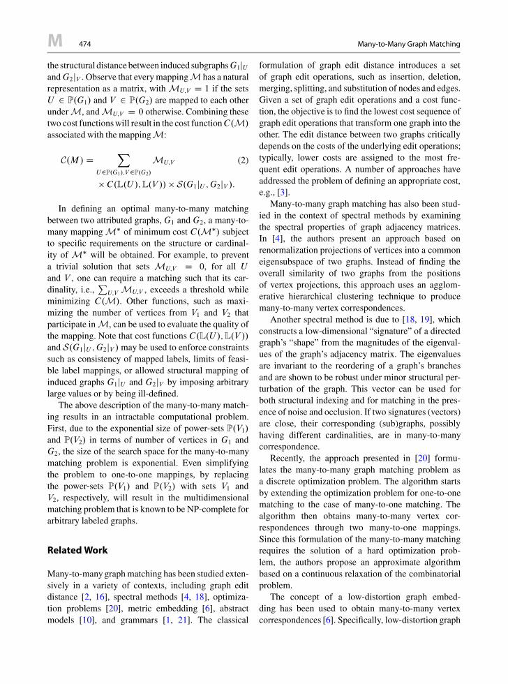
the structural distance between induced subgraphsG1jUandG2jV . Observe that every mappingM has a naturalrepresentation as a matrix, with MU;V D 1 if the setsU 2 P.G1/ and V 2 P.G2/ are mapped to each otherunder M, and MU;V D 0 otherwise. Combining thesetwo cost functions will result in the cost functionC.M/
associated with the mappingM:
C.M/ DX
U2P.G1/;V 2P.G2/
MU;V (2)
� C.L.U /;L.V // � S.G1jU ;G2jV /:
In defining an optimal many-to-many matchingbetween two attributed graphs, G1 and G2, a many-to-many mapping M� of minimum cost C.M�/ subjectto specific requirements on the structure or cardinal-ity of M� will be obtained. For example, to preventa trivial solution that sets MU;V D 0, for all U
and V , one can require a matching such that its car-dinality, i.e.,
PU;V MU;V , exceeds a threshold while
minimizing C.M/. Other functions, such as maxi-mizing the number of vertices from V1 and V2 thatparticipate in M, can be used to evaluate the quality ofthe mapping. Note that cost functions C.L.U /;L.V //
and S.G1jU ;G2jV / may be used to enforce constraintssuch as consistency of mapped labels, limits of feasi-ble label mappings, or allowed structural mapping ofinduced graphs G1jU and G2jV by imposing arbitrarylarge values or by being ill-defined.
The above description of the many-to-many match-ing results in an intractable computational problem.First, due to the exponential size of power-sets P.V1/
and P.V2/ in terms of number of vertices in G1 andG2, the size of the search space for the many-to-manymatching problem is exponential. Even simplifyingthe problem to one-to-one mappings, by replacingthe power-sets P.V1/ and P.V2/ with sets V1 andV2, respectively, will result in the multidimensionalmatching problem that is known to be NP-complete forarbitrary labeled graphs.
RelatedWork
Many-to-many graph matching has been studied exten-sively in a variety of contexts, including graph editdistance [2, 16], spectral methods [4, 18], optimiza-tion problems [20], metric embedding [6], abstractmodels [10], and grammars [1, 21]. The classical
formulation of graph edit distance introduces a setof graph edit operations, such as insertion, deletion,merging, splitting, and substitution of nodes and edges.Given a set of graph edit operations and a cost func-tion, the objective is to find the lowest cost sequence ofgraph edit operations that transform one graph into theother. The edit distance between two graphs criticallydepends on the costs of the underlying edit operations;typically, lower costs are assigned to the most fre-quent edit operations. A number of approaches haveaddressed the problem of defining an appropriate cost,e.g., [3].
Many-to-many graph matching has also been stud-ied in the context of spectral methods by examiningthe spectral properties of graph adjacency matrices.In [4], the authors present an approach based onrenormalization projections of vertices into a commoneigensubspace of two graphs. Instead of finding theoverall similarity of two graphs from the positionsof vertex projections, this approach uses an agglom-erative hierarchical clustering technique to producemany-to-many vertex correspondences.
Another spectral method is due to [18, 19], whichconstructs a low-dimensional “signature” of a directedgraph’s “shape” from the magnitudes of the eigenval-ues of the graph’s adjacency matrix. The eigenvaluesare invariant to the reordering of a graph’s branchesand are shown to be robust under minor structural per-turbation of the graph. This vector can be used forboth structural indexing and for matching in the pres-ence of noise and occlusion. If two signatures (vectors)are close, their corresponding (sub)graphs, possiblyhaving different cardinalities, are in many-to-manycorrespondence.
Recently, the approach presented in [20] formu-lates the many-to-many graph matching problem asa discrete optimization problem. The algorithm startsby extending the optimization problem for one-to-onematching to the case of many-to-one matching. Thealgorithm then obtains many-to-many vertex cor-respondences through two many-to-one mappings.Since this formulation of the many-to-many matchingrequires the solution of a hard optimization prob-lem, the authors propose an approximate algorithmbased on a continuous relaxation of the combinatorialproblem.
The concept of a low-distortion graph embed-ding has been used to obtain many-to-many vertexcorrespondences [6]. Specifically, low-distortion graph

Many-to-Many Graph Matching 475 M
M
embedding is employed to transform the problem ofmany-to-many graph matching to a many-to-manypoint matching problem in a geometric space. Thistransformation maps nodes to points and edge weightsto interpoint distances, not only simplifying the orig-inal graph representation (by removing the edges),but also retaining important local and global graphstructure; moreover, the transformation is robust underperturbation. Representing two graphs as sets of pointsreduces the many-to-many graph matching problem tothat of many-to-many point matching in the geometricspace, for which a number of efficient distribution-based similarity measures are available. The authorsuse the Earth Mover’s Distance [15] algorithm tofind such correspondences and show that the result-ing many-to-many point matching realizes the desiredmany-to-many matching between the vertices of theinput graphs.
A number of researchers, e.g., [10, 12] and [5], haveexplored many-to-many graph matching in the contextof model-based abstraction from images. The workpresented in [10] starts by forming a region adjacencygraph from each image. The approach then searchesthe space of pairwise region groupings in each graph,forming a lattice. Each input image yields a latticesuch that its bottom node represents the original regionadjacency graph and its top node represents the silhou-ette of the object. The framework defines a commonabstraction as a set of nodes, one per lattice, such thatfor a pair of nodes, their corresponding graphs are iso-morphic. The lowest common abstraction (LCA) isdefined as the common abstraction whose underlyinggraph has the maximum number of nodes. Thus, theresulting LCA carries the most informative abstractioncommon to each image. Although effective, this tech-nique does not find a match between two graphs whosecommon abstraction does not exist.
The two algorithms presented in [12] and [5] usethe many-to-many graph matching technique of [6]for automatically constructing an abstract model fromexamples. The work in [12] computes the multi-scale ridge/blob decomposition (AND-OR) graph foreach input image and obtains the many-to-many nodecorrespondences between each pair of graphs, yield-ing a matching matrix. By exploring this matrix, thealgorithm first finds features that match one-to-oneacross many pairs of input images. The many-to-manymatchings between these features are then analyzedto obtain the decompositional relations among them.
The extracted features and their relations are used toconstruct the final abstract model.
After obtaining many-to-many node correspon-dences based on [6], the algorithm in [5] computesthe abstracted medial axis graph by first computingthe averages of the corresponding pairs of subgraphsto yield the nodes in the abstracted graph, and thendefining the overall topology of the resulting abstractparts to yield the relations. Each matching pair of sub-graphs corresponds to a single node in the abstractedgraph, and two abstracted nodes are connected by anedge if the corresponding subgraphs are adjacent in theoriginal graphs. This procedure forms the basis of aniterative framework in which pairs of similar medialaxis graphs are clustered and abstracted, yielding a setof abstract medial axis graph class prototypes.
In the domain of grammars, objects are representedas variable hierarchical structures. Each part in thisrepresentation can be defined in terms of other parts,allowing an object to be modeled by its coarse-to-fineappearance. Overall, grammar-based models includ-ing AND-OR graphs support structural variability. Torepresent intra-category variation and to account formany-to-many correspondence, the grammar creates alarge number of configurations from a small vocabu-lary set. To scale to a large number of object categories,the AND-OR graph, learning, and inference algorithmsare defined recursively. Some examples of this type ofapproach include [1, 21].
Experimental Results
In this section, some example results from some ofthe many-to-many matching approaches described inthe Related Work section are illustrated. After rep-resenting silhouettes as skeleton graphs in Fig. 2,the algorithm proposed in [6] obtains many-to-manynode correspondences through metric embedding, asdiscussed earlier. Based on the many-to-many cor-respondences of this algorithm, Fig. 3 demonstratesan example for the abstract shape created by theapproach presented in [5]. The left part presents inputsilhouettes, their skeleton graphs, and many-to-manycorrespondences. The right part presents the abstractskeleton graph and its shape reconstructed from thisgraph.
Graph edit distance is another important class ofmany-to-many graph matching algorithms. Figure 4

M 476 Many-to-Many Graph Matching
Many-to-Many Graph Matching, Fig. 2 Example many-to-many correspondences computed by [6]. After representing twosilhouettes as skeleton graphs, the graphs are embedded intogeometric spaces of the same dimensionality. The embedded
points are then matched using the Earth Mover’s Distance algo-rithm. The right part illustrates the many-to-many correspon-dences between the vertices of the input graphs. Each dashedellipsoid represents a set of vertices from the original graph
Many-to-Many Graph Matching, Fig. 3 A shape abstrac-tion example of [5] based on many-to-many correspondencesobtained by [6]. The left image shows input silhouettes and theirskeleton graphs in which the same color is used to show the
corresponding parts. Using these correspondences, the abstractskeleton graph and its silhouette are created as shown on theright
Many-to-Many Graph Matching, Fig. 4 Graph edit distancealgorithms compute many-to-many correspondences of a pair ofgraphs by finding the lowest cost sequence of graph edit opera-tions needed to transform one graph into another. In the example,
same colors indicate the matching skeleton parts, while gray col-ors show spliced or contracted edges (The example is taken fromRef. [16])

Matte Extraction 477 M
M
shows the result of matching the skeleton graphs fortwo input shapes using the graph edit distance algo-rithm described in [16]. Same colors indicate thematching skeleton parts while gray colors show splicedor contracted edges. Observe that the many-to-manycorrespondences are intuitive in these figures.
References
1. Bunke H (1982) Attributed graph grammars and their appli-cation to schematic diagram interpretation. IEEE TransPattern Anal Mach Intell 4:574–582
2. Bunke H (1997) On a relation between graph edit distanceand maximum common subgraph. Pattern Recognit Lett18(8):689–694
3. Bunke H, Shearer K (1998) A graph distance metric basedon the maximal common subgraph. Pattern Recognit Lett19:255–259
4. Caelli T, Kosinov S (2004) An eigenspace projection clus-tering method for inexact graph matching. IEEE TransPattern Anal Mach Intell 26:515–519
5. Demirci F, Shokoufandeh A, Dickinson S (2009) Skeletalshape abstraction from examples. IEEE Trans Pattern AnalMach Intell 31:944–952
6. Demirci F, Shokoufandeh A, Keselman Y, Bretzner L,Dickinson S (2006) Object recognition as many-to-manyfeature matching. Int J Comput Vis 69(2):203–222
7. Dickinson S (2009) The evolution of object categorizationand the challenge of image abstraction. In: Dickinson S,Leonardis A, Schiele B, Tarr M (eds) Object categoriza-tion: computer and human vision perspectives. CambridgeUniversity Press, New York, pp 1–37
8. Ferrari V, Jurie F, Schmid C (2010) From images toshape models for object detection. Int J Comput Vis 87(3):284–303
9. Fischler MA, Eschlager RA (1973) The representationand matching of pictorial structures. IEEE Trans Comput22(1):67–92
10. Keselman Y, Dickinson S (2005) Generic model abstrac-tion from examples. IEEE Trans Pattern Anal Mach Intell27(7):1141–1156
11. Lamdan Y, Schwartz J, Wolfson H (1990) Affine invariantmodel-based object recognition. IEEE Trans Rob Autom6(5):578–589
12. Levinshtein A, Sminchisescu C, Dickinson S (2005) Learn-ing hierarchical shape models from examples.In: Proceed-ings of the EMMCVPR, St. Augustine. Springer, Berlin,pp 251–267
13. Lowe D (1985) Perceptual organization and visual recogni-tion. Academic, Norwell
14. Lowe D (2004) Distinctive image features from scale-invariant keypoints. Int J Comput Vis 60(2):91–110
15. Rubner Y, Tomasi C, Guibas LJ (2000) The earth mover’sdistance as a metric for image retrieval. Int J Comput Vis40(2):99–121
16. Sebastian T, Klein P, Kimia B (2004) Recognition of shapesby editing their shock graphs. IEEE Trans Pattern AnalMach Intell 26:550–571
17. Shokoufandeh A, Bretzner L, Macrini D, Demirci MF,Jönsson C, Dickinson S (2006) The representation andmatching of categorical shape. Comput Vis Image Underst103(2):139–154
18. Shokoufandeh A, Macrini D, Dickinson S, Siddiqi K,Zucker SW (2005) Indexing hierarchical structures usinggraph spectra. IEEE Trans Pattern Anal Mach Intell27(7):1125–1140
19. Siddiqi K, Shokoufandeh A, Dickinson S, Zucker S (1999)Shock graphs and shape matching. Int J Comput Vis 30:1–24
20. Zaslavskiy M, Bach F, Vert J (2010) Many-to-manygraph matching: a continuous relaxation approach. LectureNotes in Computer Science, http://arxiv.org/abs/1004.4965,DBLP, http://dblp.uni-trier.de 6323:515–530
21. Zhu S, Mumford D (2006) A stochastic grammar of images.Found Trends Comput Graph Vis 2:259–362
Matte Extraction
Jiaya JiaDepartment of Computer Science and Engineering,The Chinese University of Hong Kong, Shatin, N.T.,Hong Kong, China
Synonyms
Digital matting; Pulling a matte
Definition
An alpha matte has the same size as the input image.It contains respective weights to linearly blend latentforeground and background colors for each pixel toform the observed color. Estimating the alpha mattetogether with the foreground color image is generallyreferred to as matte extraction or digital matting.
Background
Classifying each pixel in an input image to either fore-ground or background is called binary segmentation,which is a fundamental computer vision problem. Dig-ital matting relaxes the hard separation assumption

M 478 Matte Extraction
and takes ubiquitous foreground and backgroundcolor blending in image formation, which happensalong almost all object boundaries, into consideration.Results from matte extraction can be used to generatea new composite.
Color blending in natural images has a varietyof causes, such as color interpolation during imageproduction and light photons received by the cam-era sensor containing both background and foregroundcolor for some pixels. Without additional informa-tion, digital matting is an ill-posed problem with manyunknowns. So generally, either multiple frames aretaken or a certain amount of user interaction is involvedto sample foreground and background color in imageand video matting.
Theory
In the digital matting framework, separating the back-ground image B and foreground image F with respectto an alpha matte ˛ from an input natural image I isexpressed as
I D ˛F C .1 � ˛/B: (1)
If ˛.x; y/ D 1, the pixel with coordinate .x; y/ is def-initely in the foreground. ˛.x; y/ being 0 defines anabsolutely background pixel. ˛.x; y/ can also be inbetween 0 and 1, indicating a certain level of colormixing. Digital matting aims to estimate ˛ and F
(sometimes also B) from I . Existing methods followone of the following lines.
Blue ScreenMattingBlue screen matting [1], which is widely employedin movie and commercial production, needs to set upa controlled environment and uses a single or multi-ple constant-color backgrounds (as shown in Fig. 1).The blue screen matting problem is directly solv-able. Its triangular matting technique, which capturesimages with two backgrounds containing differentshades of the backing color, is particularly noteworthybecause a closed-form solution exists. This techniquecan produce very accurate matting results usable asground truth data. Blue screen matting can be appliedin a frame-by-frame fashion to video foreground objectextraction.
Natural Image MattingIn natural image matting, background B is generallyunknown and possibly contains complex structures.In this case, simultaneously estimating ˛, F , and B
becomes an ill-posed problem. Several methods [3–5]need user input of additional segmentation informa-tion to constrain it. Trimap is a popular format thatpartitions the image into three regions, i.e., “defi-nitely foreground” (DF for short), “definitely back-ground” (DB for short), and “unknown region”, asshown in Fig. 2b. In DF and DB, ˛ is set to 1 and 0,respectively. Digital matting only estimates ˛, togetherwith the foreground and background color, in theunknown region by gathering color information fromDF and DB.
There have been several methods proposed to sam-ple color from DF and DB. In knockout [6], F iscomputed as the weighted average of foreground coloralong the perimeter of the DF region. B is computedsimilarly but with a final refinement step. Ruzon andTomasi [3] sample F and B from local windows andthen parameterize them as a mixture of unorientedGaussians. Alpha values are computed by maximiz-ing a function that interpolates the mean and varianceof the Gaussians. Bayesian matting [4] gathers colorsamples from DF and DB using sliding windows andfits them with oriented Gaussian distributions. A max-imum a posteriori (MAP) estimation of ˛, F , and B
is applied. The final ˛ values are chosen from theforeground and background color pairs that maximizethe probability. Global Poisson matting [5] contributesa gradient-domain alpha matte estimation. When thecondition of locally smooth color change in DF andDB is violated, user interaction is involved to improvethe matting result with the supply of a group of filters.
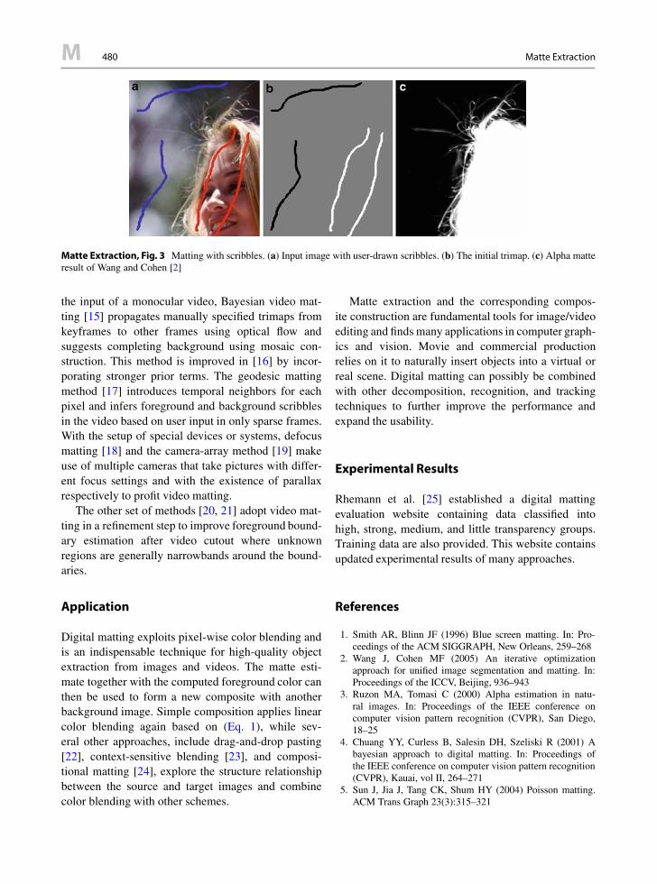
The quality of results of these methods partlydepends on how accurate the trimap is since coloris sampled and the alpha matte is estimated withinwindows. Many later approaches instead require theuser to only draw several foreground and backgroundscribbles to coarsely indicate DF and DB and leaveall unspecified pixels in the unknown region. Thisscheme simplifies user interaction but provides looserconstraints for digital matting, as shown in Fig. 3.Representative work that can robustly solve foralpha mattes based on it includes (1) the iterative-optimization method [2], which samples color fromuser-drawn scribbles, builds the Markov RandomField (MRF), and solves for segmentation and matte

Matte Extraction 479 M
M
Matte Extraction, Fig. 1Blue screen matting [1]. (a)Object against knownconstant blue. (b) Objectagainst constant black.(c) Pulled foreground. (d)New composite
Input
a b c
Trimap Alpha matte
Matte Extraction, Fig. 2 A trimap matting example. (a) Inputimage. (b) The user-provided trimap where definitely foregroundand background are in white and black, respectively. The gray
pixels are unknown ones. (c) Alpha matte estimate by globalPoisson matting
extraction using belief propagation, and (2) closed-form matting [7] that introduces a color line modeland based on it derives a quadratic cost function onlyinvolving ˛ and a matting Laplacian, enabling linearoptimization. In addition, Rhemann et al. [8] extracthigh-resolution mattes by trimap segmentation andby employing gradient preserving alpha priors. Thesoft-scissor method of Wang et al. [9] can achieve real-time matting along with user painting the foregroundboundary.
There are also automatic image matting meth-ods. A soft color segmentation method was proposedin [26], where a global objective function is mod-eled by global and local parameters. These param-eters are alternately optimized until convergence. Itcan be applied to matting without intensive userinteraction. Spectral matting [10] is a single imageapproach. It shows that the smallest eigenvectors of
the matting Laplacian span individual matting com-ponents, making their estimation equivalent to findinglinear transformation of the eigenvectors. Flash mat-ting [11] captures a pair of flash/no-flash images andassumes only the foreground region is lit by flash. Thismethod can automatically extract foreground in a jointBayesian matting framework.
Albeit some inevitable limitations as described inrespective papers, all the above techniques advanceimage matting from different aspects. Other recom-mended readings also include [12–14].
Video MattingDigital matting was extended to videos in vari-ous ways. Typical video matting methods deal withforeground regions with hair, trees, or smoke, wherecolor blending exists for a large amount of pixels.To preserve temporal coherence among frames, with
M 480 Matte Extraction
Matte Extraction, Fig. 3 Matting with scribbles. (a) Input image with user-drawn scribbles. (b) The initial trimap. (c) Alpha matteresult of Wang and Cohen [2]
the input of a monocular video, Bayesian video mat-ting [15] propagates manually specified trimaps fromkeyframes to other frames using optical flow andsuggests completing background using mosaic con-struction. This method is improved in [16] by incor-porating stronger prior terms. The geodesic mattingmethod [17] introduces temporal neighbors for eachpixel and infers foreground and background scribblesin the video based on user input in only sparse frames.With the setup of special devices or systems, defocusmatting [18] and the camera-array method [19] makeuse of multiple cameras that take pictures with differ-ent focus settings and with the existence of parallaxrespectively to profit video matting.
The other set of methods [20, 21] adopt video mat-ting in a refinement step to improve foreground bound-ary estimation after video cutout where unknownregions are generally narrowbands around the bound-aries.
Application
Digital matting exploits pixel-wise color blending andis an indispensable technique for high-quality objectextraction from images and videos. The matte esti-mate together with the computed foreground color canthen be used to form a new composite with anotherbackground image. Simple composition applies linearcolor blending again based on (Eq. 1), while sev-eral other approaches, include drag-and-drop pasting[22], context-sensitive blending [23], and composi-tional matting [24], explore the structure relationshipbetween the source and target images and combinecolor blending with other schemes.
Matte extraction and the corresponding compos-ite construction are fundamental tools for image/videoediting and finds many applications in computer graph-ics and vision. Movie and commercial productionrelies on it to naturally insert objects into a virtual orreal scene. Digital matting can possibly be combinedwith other decomposition, recognition, and trackingtechniques to further improve the performance andexpand the usability.
Experimental Results
Rhemann et al. [25] established a digital mattingevaluation website containing data classified intohigh, strong, medium, and little transparency groups.Training data are also provided. This website containsupdated experimental results of many approaches.
References
1. Smith AR, Blinn JF (1996) Blue screen matting. In: Pro-ceedings of the ACM SIGGRAPH, New Orleans, 259–268
2. Wang J, Cohen MF (2005) An iterative optimizationapproach for unified image segmentation and matting. In:Proceedings of the ICCV, Beijing, 936–943
3. Ruzon MA, Tomasi C (2000) Alpha estimation in natu-ral images. In: Proceedings of the IEEE conference oncomputer vision pattern recognition (CVPR), San Diego,18–25
4. Chuang YY, Curless B, Salesin DH, Szeliski R (2001) Abayesian approach to digital matting. In: Proceedings ofthe IEEE conference on computer vision pattern recognition(CVPR), Kauai, vol II, 264–271
5. Sun J, Jia J, Tang CK, Shum HY (2004) Poisson matting.ACM Trans Graph 23(3):315–321

Maximum Likelihood Estimation 481 M
M
6. Berman A, Vlahos P, Dadourian A (2000) Comprehen-sive method for removing from an image the backgroundsurrounding a selected object. US Patent 6,134,345
7. Levin A, Lischinski D, Weiss Y (2006) A closed form solu-tion to natural image matting. In: Proceedings of the IEEEconference on computer vision pattern recognition (CVPR),New York, 61–68
8. Rhemann C, Rother C, Rav-Acha A, Sharp T (2008) Highresolution matting via interactive trimap segmentation. In:Proceedings of the IEEE conference on computer visionpattern recognition (CVPR), Anchorage
9. Wang J, Agrawala M, Cohen MF (2007) Soft scissors:an interactive tool for realtime high quality matting. In:Proceedings of the ACM SIGGRAPH, San Diego
10. Levin A, Rav-Acha A, Lischinski D (2008) Spec-tral matting. IEEE Trans Pattern Anal Mach Intell 30:1699–1712
11. Sun J, Li Y, Kang SB, Shum HY (2006) Flash matting. In:Proceedings of the SIGGRAPH, Boston, 772–778
12. Grady L, Schiwietz T, Aharon S, Westermann R (2005) Ran-dom walks for interactive alpha-matting. In: Proceedings ofthe VIIP, 423–429
13. Wang J, Cohen MF (2007) Image and video matting: asurvey. Found Trends Comput Graph Vis 3:97–175
14. Rhemann C, Rother C, Kohli P, Gelautz M (2010) A spa-tially varying psf-based prior for alpha matting. In: Pro-ceedings of the IEEE conference on computer vision patternrecognition (CVPR), San Francisco, 2149–2156
15. Chuang YY, Agarwala A, Curless B, Salesin DH, Szeliski R(2002) Video matting of complex scenes. In: Proceedings ofthe SIGGRAPH, San Antonio, 243–248
16. Apostoloff N, Fitzgibbon A (2004) Bayesian video mat-ting using learnt image priors. Comput Vis Pattern Recognit1:407–414
17. Bai X, Sapiro G (2009) Geodesic matting: a framework forfast interactive image and video segmentation and matting.Int J Comput Vis 82:113–132
18. McGuire M, Matusik W, Pfister H, Hughes JF, Durand F(2005) Defocus video matting. In: Proceedings of the ACMSIGGRAPH, Los Angeles, 567–576
19. Joshi N, Matusik W, Avidan S (2006) Natural video mattingusing camera arrays. In: Proceedings of the SIGGRAPH,Boston, 779–786
20. Li Y, Sun J, Shum HY (2005) Video object cut and paste.In: Proceedings of the ACM SIGGRAPH, Los Angeles,595–600
21. Wang J, Bhat P, Colburn RA, Agrawala M, Cohen MF(2005) Interactive video cutout. In: Proceedings of the ACMSIGGRAPH, Los Angeles, 585–594
22. Jia J, Sun J, Tang CK, Shum HY (2006) Drag-and-droppasting. In: Proceedings of the ACM SIGGRAPH, Boston,631–637
23. Lalonde JF, Hoiem D, Efros AA, Rother C, Winn J, Crim-inisi A (2007) Photo clip art. In: Proceedings of the ACMSIGGRAPH, San Diego
24. Wang J, Cohen MF (2007) Simultaneous matting andcompositing. In: Proceedings of the IEEE confer-ence on computer vision pattern recognition (CVPR),Minneapolis
25. Rhemann C, Rother C, Wang J, Gelautz M, Kohli P, Rott P(2009) A perceptually motivated online benchmark for
image matting. In: Proceedings of the IEEE conference oncomputer vision pattern recognition (CVPR), Miami
26. Tai Y-W, Jia J, Tang C-K (2007) Soft color segmentation andits applications. IEEE Trans. Pattern Anal. Mach. Intell. 29,9 (September 2007), 1520–1537
Maximum Likelihood Estimation
Thomas BroxDepartment of Computer Science, University ofFreiburg, Freiburg, Germany
Synonyms
Maximum likelihood estimator
Definition
Maximum likelihood estimation seeks to estimatemodel parameters that best explain some given, inde-pendent measurements according to a noise model.
Background
Many problems in computer vision can be formulatedas finding the parameters of a predefined model givenmeasurements or training examples.
For example in image segmentation one may wantto describe a region by a simple region model, e.g., bya constant intensity value �. There are many measure-ments, namely all the pixel intensities in the region.Assuming that these pixel intensities are independentlygenerated from the constant intensity model accordingto a Gaussian distribution, the goal is to find the mostlikely parameter � given these measurements. In thissimple example, the optimal parameter � is the meanof all intensities.
There are many more similar problems in computervision, for instance, in the scope of optical flow estima-tion, camera calibration, image denoising, or patternrecognition. In the special case of a Gaussian noisemodel, maximum likelihood estimation comes downto a least squares approach.
Maximum likelihood estimation is often criticizedbecause it ignores a-priori information, which can beinterpreted as assuming a uniform prior density on theparameter space. This becomes especially problematic

M 482 Maximum Likelihood Estimator
when the model is described by many parameters andthere are relatively few measurements. In cases wheregood a-priori assumptions can be made, maximumlikelihood estimation should be replaced by maximuma-posteriori estimation, which takes the prior densityinto account.
Theory
Given a probabilistic model that is described by aparameter vector w 2 R
D and given N indepen-dent measurements xn 2 R
K , N � D, one aims atmaximizing the likelihood
p .x1; : : : ; xN jw/ DNY
nD1
p .xnjw/ : (1)
For numerical reasons, rather than maximizing thisprobability, it is common to maximize its logarithm,the so-called log-likelihood:
w� D argmaxw
logp.x1; : : : ; xN jw/
D argmaxw
NX
nD1
logp.xnjw/: (2)
Application
Applying this to a simple regression problem, wherea line is to be fitted to a couple of points, one has theconstraints
w1x1;n C w2 D x2;n; n D 1; : : : ; N: (3)
Assuming a Gaussian distribution with constantcovariance yields
NX
nD1
logp.xnjw/ /NX
nD1
.w1x1;n C w2 � x2;n/2: (4)
The connection to least squares estimation can be seenimmediately, but one could as well assume a Laplacedistribution, which is more robust to outliers among the
measurements and would lead to
NX
nD1
logp.xnjw/ /NX
nD1
jw1x1;n C w2 � x2;nj: (5)
A necessary condition for a maximum of this expres-sion is that the gradient with respect to the parametervector must vanish:
@@w1
PNnD1 jw1x1;n C w2 � x2;nj D 0
@@w2
PNnD1 jw1x1;n C w2 � x2;nj D 0
(6)
leading to the nonlinear system
PNnD1
1
2
.w1x1;n C w2 � x2;n/x1;n
jw1x1;n C w2 � x2;nj D 0
PNnD1
1
2
.w1x1;n C w2 � x2;n/
jw1x1;n C w2 � x2;nj D 0;
(7)
which can be solved by iteratively keeping the denom-inators fixed, solving the resulting linear system andupdating the denominator. Gaussian distributions leadto linear systems that can be solved directly. Moredetails and examples on maximum likelihood estima-tion can be found in [1, 2].
References
1. Duda RO, Stork DG, Hart PE (2000) Pattern classification,2nd edn. Wiley, New York
2. Bishop CM (2006) Pattern recognition and machine learning.Springer
Maximum Likelihood Estimator
�Maximum Likelihood Estimation
Mesostructure
�Bidirectional Texture Function and 3D Texture
Mirrors 483 M
M
Methods of Image Recognition ina Low-Dimensional Eigenspace
�Eigenspace Methods
Microgeometry
�Bidirectional Texture Function and 3D Texture
Micro Scale Structure
�Surface Roughness
Mirrorlike Reflection
�Specularity, Specular Reflectance
Mirrors
Jürgen BeyererFraunhofer Institute of Optronics,System Technologies and Image Exploitation IOSB,Karlsruhe, Germany
Definition
A mirror is an optical device used for beam-forming orimaging based on the directional reflection of electro-magnetic radiation.
Background
Computer vision applications apply mirrors in atwofold manner: for optical imaging and for illumina-tion purposes. Furthermore, mirrors themselves couldbe test objects in visual inspection systems. This leads,with regard to the 3D shape of the mirror, to the shape-from-specular-reflection problem, and in the context ofvisual inspection systems to deflectometry.
Theory and Application
Mirrors consist of a smooth substrate with a metal coat-ing (e.g., Au, Ag, Al) and/or dielectric layers. In thecase of a surface mirror, the reflection takes place at ametal coating on the front side that has to be protectedagainst scratches. The main advantage of a surface mir-ror is the lack of beam displacement due to the glasssubstrate. Alternatively, the backside of a glass sub-strate can be coated with a metal layer and with anadditional protection against humidity and mechanicaldamage. Backside mirrors are usually more robust thansurface mirrors, but lack their optical characteristicsmentioned above.
The physical effect leading to the reflection of elec-tromagnetic waves on metal surfaces can be simplydescribed as “short circuit” of the electrical field.
Dielectric mirrors are composed of multiple thinlayers of dielectric materials. They exhibit very highreflectance values, whereas the reflectance dependson wavelength, incident angle, and polarization.Advanced multilayer structure designs can be used toobtain certain functionality [10]:• A broader reflection bandwidth• A combination of desirable reflectivity values in
different wavelength ranges• Special polarization properties (for non-normal
incidence, thin-film polarizers, polarizing beamsplitters)
• Non-polarizing beam splitters• Edge filters, e.g., long-pass filters, high-pass filters,
band-pass filters• Tailored chromatic dispersion propertiesSuch mirrors are especially used in laser applications.
Furthermore, thin metal layers allow semitranspar-ent mirrors to be realized for coaxial illumination.
The electromagnetic theory of light is fundamen-tal for the physical understanding of specular reflec-tions [3]. Thereby, the law of reflection describesthe geometric aspects, and the Fresnel equations thereflection coefficients, i.e., the radiometric behavior.
The law of reflection states the relationship of theincident si and reflected sr light rays with the normalof the specular surface n :
si � n D sr � n ; (1)
with ksik D ksrk D knk D 1.
M 484 Mirrors
Equation 1 leads, with ksi � nk D sin �i D sin �r Dksr � nk, directly to the following two conditions:• The angle of the incident ray equals that of the
reflected ray .�i D �r/.• The incident and reflected ray are coplanar with the
surface normal.In computer graphics and ray-tracing the law of
reflection is often used in the form of a Householdertransformation:
sr D H si with H WD I � 2nnT ; (2)
with the identity matrix I .The bidirectional reflectance distribution function
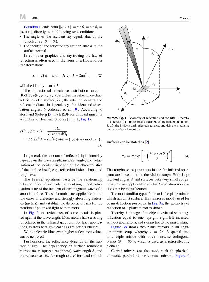
(BRDF; �.�i; 'iI �r; 'r/) describes the reflectance char-acteristics of a surface, i.e., the ratio of incident andreflected radiance in dependency of incident and obser-vation angles, Nicodemus et al. [9]. According toHorn and Sjoberg [5] the BRDF for an ideal mirror isaccording to Horn and Sjoberg [5] (c.f., Fig. 1):
�.�i; 'iI �r; 'r/ D dLr
Li cos �i d˝i
D 2 ı.sin2�r � sin2�i/ ı.'r � ..'i C �/ mod 2�// :
(3)
In general, the amount of reflected light intensitydepends on the wavelength, incident angle, and polar-ization of the incident light and on the characteristicsof the surface itself, e.g., refraction index, shape androughness.
The Fresnel equations describe the relationshipbetween reflected intensity, incident angle, and polar-ization state of the incident electromagnetic wave of asmooth surface. These formulas are applicable in thetwo cases of dielectric and strongly absorbing materi-als (metals), and establish the theoretical basis for thecreation of polarized light with mirrors.
In Fig. 2, the reflectance of some metals is plot-ted against the wavelength. Most metals have a strongreflectance in the infrared spectrum. For laser applica-tions, mirrors with gold coatings are often sufficient.
With dielectric films even higher reflectance valuescan be achieved.
Furthermore, the reflectance depends on the sur-face quality. The dependency on surface roughness� (root-mean-squared roughness), wavelength �, andthe reflectances R� for rough and R for ideal smooth
x
y
z
dLr
dEi
dW i
qiqr
jr
ji
Li
dA
Mirrors, Fig. 1 Geometry of reflection and the BRDF, therebyd˝i denotes an infinitesimal solid angle of the incident radiation,Li; Lr the incident and reflected radiance, and dEi the irradianceon the surface element dA
surfaces can be stated as [2]:
R� D R exp
"��4�� cos �i
�
�2#: (4)
The roughness requirements in the far-infrared spec-trum are lower than in the visible range. With largeincident angles �i and surfaces with very small rough-ness, mirrors applicable even for X-radiation applica-tions can be manufactured.
The most familiar type of mirror is the plane mirror,which has a flat surface. This mirror is mostly used forbeam deflection purposes. In Fig. 3a, the geometry ofreflection on a plane mirror is shown.
Thereby the image of an object is virtual with mag-nification equal to one, upright, right-left inversed,without aberrations, and symmetric to the mirror plane.
Figure 3b shows two plane mirrors in an angu-lar mirror setup, whereby � D 2ı. A special caseis a triple mirror with three pairwise orthogonalplanes (ı D 90ı), which is used as a retroreflectingelement.
Curved mirrors are also used, such as spherical,ellipsoid, paraboloid, or conical mirrors. Figure 4

Mirrors 485 M
M
Mirrors, Fig. 2 Reflectancevs. wavelength curves for gold(Au), silver (Ag), and copper(Cu) at normal incidence [1]
Wavelength
Au
Ag
Cu
100nm 1mm
1
0.8
0.6
0.4
0.2
Ref
lect
ance
10mm
Mirrors, Fig. 3 Plane (a) andangular mirror (b) Mirror
a b
Object
δ
γ
Virtual image
Observation point
shows convex and concave mirrors for optical imaging.The focal distance of a spherical mirror with radius ris given by:
f D r
2: (5)
The mirror equation:
2
rD 1
sC 1
s0(6)
describes the relationship between object and imagedistances .s; s0/ with the mirror radius r .
A big advantage of mirrors above lenses is the lackof aberrations, but with the disadvantage of highercentering and adjustment requirements.
Torrance and Sparrow [13] and Phong [11] have,among many others, introduced surface models whichcan be used to describe specular reflections. Modeling
of mirrors or partially reflecting surfaces is of ongoinginterest for computer graphics applications.
Open Problems
The main principle for the visual inspection of mirrorsis to use a highly controllable environment, where ascreen presenting a well-designed pattern is observedvia the specular reflecting surface. Knowing that pat-tern, it is possible to inspect the surface qualitativelyand – at least with certain additional knowledge – toreconstruct the surface quantitatively. This reconstruc-tion problem is ill-posed in a mathematical sense,and several regularization approaches have been pro-posed. The reconstruction of large and complex formedmirrors is still a challenge in the field of computervision [6–8, 14, 15].
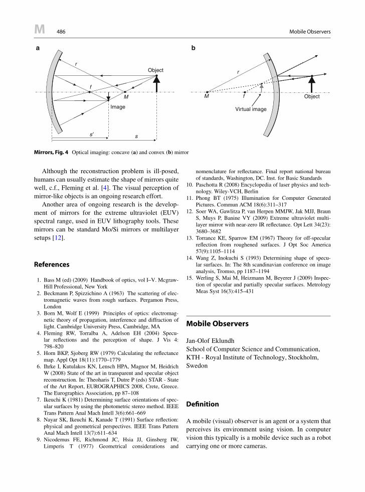
M 486 Mobile Observers
b
M f
r
Object
Virtual image
M
f
rObject
a
Image
s′ s
Mirrors, Fig. 4 Optical imaging: concave (a) and convex (b) mirror
Although the reconstruction problem is ill-posed,humans can usually estimate the shape of mirrors quitewell, c.f., Fleming et al. [4]. The visual perception ofmirror-like objects is an ongoing research effort.
Another area of ongoing research is the develop-ment of mirrors for the extreme ultraviolet (EUV)spectral range, used in EUV lithography tools. Thesemirrors can be standard Mo/Si mirrors or multilayersetups [12].
References
1. Bass M (ed) (2009) Handbook of optics, vol I–V. Mcgraw-Hill Professional, New York
2. Beckmann P, Spizzichino A (1963) The scattering of elec-tromagnetic waves from rough surfaces. Pergamon Press,London
3. Born M, Wolf E (1999) Principles of optics: electromag-netic theory of propagation, interference and diffraction oflight. Cambridge University Press, Cambridge, MA
4. Fleming RW, Torralba A, Adelson EH (2004) Specu-lar reflections and the perception of shape. J Vis 4:798–820
5. Horn BKP, Sjoberg RW (1979) Calculating the reflectancemap. Appl Opt 18(11):1770–1779
6. Ihrke I, Kutulakos KN, Lensch HPA, Magnor M, HeidrichW (2008) State of the art in transparent and specular objectreconstruction. In: Theoharis T, Dutre P (eds) STAR - Stateof the Art Report, EUROGRAPHICS 2008, Crete, Greece.The Eurographics Association, pp 87–108
7. Ikeuchi K (1981) Determining surface orientations of spec-ular surfaces by using the photometric stereo method. IEEETrans Pattern Anal Mach Intell 3(6):661–669
8. Nayar SK, Ikeuchi K, Kanade T (1991) Surface reflection:physical and geometrical perspectives. IEEE Trans PatternAnal Mach Intell 13(7):611–634
9. Nicodemus FE, Richmond JC, Hsia JJ, Ginsberg IW,Limperis T (1977) Geometrical considerations and
nomenclature for reflectance. Final report national bureauof standards, Washington, DC. Inst. for Basic Standards
10. Paschotta R (2008) Encyclopedia of laser physics and tech-nology. Wiley-VCH, Berlin
11. Phong BT (1975) Illumination for Computer GeneratedPictures. Commun ACM 18(6):311–317
12. Soer WA, Gawlitza P, van Herpen MMJW, Jak MJJ, BraunS, Muys P, Banine VY (2009) Extreme ultraviolet multi-layer mirror with near-zero IR reflectance. Opt Lett 34(23):3680–3682
13. Torrance KE, Sparrow EM (1967) Theory for off-specularreflection from roughened surfaces. J Opt Soc America57(9):1105–1114
14. Wang Z, Inokuchi S (1993) Determining shape of specu-lar surfaces. In: The 8th scandinavian conference on imageanalysis, Tromso, pp 1187–1194
15. Werling S, Mai M, Heizmann M, Beyerer J (2009) Inspec-tion of specular and partially specular surfaces. MetrologyMeas Syst 16(3):415–431
Mobile Observers
Jan-Olof EklundhSchool of Computer Science and Communication,KTH - Royal Institute of Technology, Stockholm,Swedon
Definition
A mobile (visual) observer is an agent or a system thatperceives its environment using vision. In computervision this typically is a mobile device such as a robotcarrying one or more cameras.

Mobile Observers 487 M
M
Background
Gibson [1] claimed that a mobile observer is a pre-requisite for natural vision. He discriminated betweenambient or ambulatory vision, when the observercan move its head or body, and snapshot or aper-ture vision in cases when one or several images arerecorded momentarily at certain fixation points. Allthose aspects are treated in computer vision, althoughcurrent trends are on processing static images in thespirit of snapshot or aperture vision. Computer visionresearchers began to study visual motion in the 1970s,when it became possible to connect video cameras tocomputers. This work did not really concern mobileobservers, but such existed even earlier, when cam-eras were used as input devices to robots, e.g., in thework on “Shakey” [2]. Nowadays, mobile observersmost often occur in the context of mobile robots, butrecent developments on wearable vision have widenedthe interest in the topic. Ambient vision is what youhave for instance in the case of pan-tilt heads, whichare used in a large range of applications.
Theory
There have been attempts to find the notions of activeand mobile observers theoretically. In biological visionGibson’s work is of a landmark nature, but there aremany other proposals as well, e.g., relating to func-tionalism [3]. In computer vision the problem has beenconsidered from the point of view of active vs. passivevision [4–6]. In [7–9] the theoretical aspects are moredirectly addressed. However, even with these attempts,one can hardly say that there exists any completetheory for a mobile observer.
Problems and Applications
The mobile observer obtains a stream or sequence ofimages as input rather than single images. This pro-vides rich information about the environment as well asof the movements of the observer. However, observermotion also implies that there is image motion inalmost every point in the sequence. In a static world,observer motion creates essentially all the variationsover time in the images, i.e., those that are due tochange of viewpoint and not, e.g., in illumination. Ifthere are things in the environment that also move, thetwo types of motion are confounded in the images.
A mobile observer can derive (static) scene geom-etry through structure-from-motion algorithms. More-over, ego-motion, i.e., the motion of the observer,can be estimated. Generally such methods assume astatic background that is prominent in the field ofview. Independently moving objects can then also bedetected, and under certain conditions their motion canbe estimated. Ego-motion estimation obviously playsan important role here. There are many types of algo-rithms for this, e.g., based on optical flow, monocularor binocular feature tracking, or image stabilization.There also exist algorithms for using omnidirectionalor composite cameras, which highlights the fact thateffects of ego-motion are manifested in a wide fieldof view. For instance, small rotations of an observermoving straight ahead can be estimated from periph-eral flow, something that is useful in driving and inguiding of autonomous robots.
A mobile observer can be active or passive. Inthe first case, it purposively guides its motion and/orthe way it directs its gaze on the basis of tasks itis involved in and as a reaction to what it observes.Gaze control and fixation in dynamic situations havebeen studied extensively in the field of active vision.In some cases these mechanisms have been used tocontrol observer motion, e.g., for exploring a scene oran object and to facilitate recognition. Then viewpointplanning becomes an issue. However, a more gen-eral case is when the observer motion is only looselydependent of what is seen, except for possible controlof gaze. For instance, a mobile observer can inducedepth cues through parallax by (small) camera motionsthat are not pure rotations. Another example is givenby a robot moving from one point to another whileobserving an object along its path, analogously to aperson riding in a car. Many applications contain ele-ments of both active and passive observations, forinstance in robot navigation including obstacle avoid-ance and mapping (as in SLAM), hand-eye control ingrasping and manipulation, and in general for an ambu-lant observer, such as those studied in the context ofwearable or egocentric vision.
Open Problems
The study of mobile observers from a computa-tional perspective involves a broad range of problemstraditionally addressed in computer vision. However,

M 488 MoCap
there are certain issues that become central. Forinstance, the correspondence problem is ubiquitous. Inapplications such as those described above, the tightconnection between perception and action is apparent.Visual sensing involving motor control raises prob-lems on time criticality and real-time computations[9]. Other problems arise because the mobile observercontinuously samples the visual world. Meaningfulbehavior based on the huge amounts of informationrequires methods for attention and visual search. Inall, although some of the problems encountered in thestudy of mobile observers largely overlap those gener-ally treated in computer vision, there are others that arespecific to this area.
References
1. Gibson JJ (1979) The ecological approach to visual percep-tion. Houghton Mifflin, Boston
2. http://www.ai.sri.com/shakey/3. O’Regan JK, Noe A (2001) A sensorimotor account of vision
and visual consciousness. Behav Brain Sci 24:939–10314. Bajcsy R (1985) Active perception vs. passive perception. In:
Proceedings of the 3rd IEEE workshop on computer vision,Bellaire. IEEE CS Press, pp 55–59
5. Aloimonos Y, Weiss I, Bandyopadhyay A (1987) Activevision. In: Proceedings of the 1st ICCV, London. IEEE CSPress, pp 35–54
6. Ballard DH (1991) Animate vision. Artif Intell 48:57–867. Tsotsos JK (1992) On the relative complexity of active vs.
passive visual search. Int J Comput Vis 7:127–1418. Bennett BM, Hoffman DD, Prakash C (1989) Observer
mechanics: a formal theory of perception. Academic, SanDiego
9. Soatto S (2011) Steps toward a theory of visual information.CoRR. MIT, Cambridge
MoCap
�Motion Capture
Model-Based Object Recognition
Min Sun and Silvio SavareseDepartment of Electrical and Computer Engineering,University of Michigan, Ann Arbor, MI, USA
Synonyms
Object models; Object parameterizations; Object rep-resentations; Visual patterns
Related Concepts
�Human Pose Estimation; �Object Class Recognition(Categorization); �Object Detection
Definition
Model-based object recognition addresses the problemof recognizing objects from images by means of a suit-able mathematical model that is used to describe theobject.
Background
In model-based object recognition, an object model istypically defined so as to capture object’s geometri-cal and appearance properties at the appropriate levelof specificity. For instance, an object model can bedesigned to recognize a generic “face” as opposed to“someone’s face” or vice versa. In the former case,which is often referred to as the object categorizationproblem, the main challenge is to design models thatare capable of retaining key visual properties for rep-resenting an object category, such as a “face,” at theappropriate level of abstraction. Such models can bethen used to recognize novel object instances from aquery image. Moreover, a model must be able to gen-eralize across variations in the object’s visual charac-teristics due to viewpoint and illumination changes aswell as due to occlusions or deformations. Meeting allof these desiderata can be extremely challenging. Thismakes object recognition an open, yet key, problem incomputer vision.
Object Models for Recognition
The design of an object model must reflect its ability to(i) capture geometrical and appearance characteristicsof the object at the appropriate level of specificity and(ii) generalize across variations in viewpoint, illumina-tion, occlusions, and deformations. The complexity ofthe representation can be reduced by making assump-tions on the type of object specificity or the degreeof viewpoint, occlusions, and deformation variability.Ultimately, the strategy in designing an object modelwill depend on the relevant application scenario.

Model-Based Object Recognition 489 M
M
Object models that are designed to recognizeobjects at the highest level of specificity – e.g., “myface” as opposed to “a face” – are often referred toas single-instance object models. These models arecapable of recognizing a specific object instance whileguaranteeing the ability to handle occlusions and alarge degree of viewpoint variability. Research on 3Dobject recognition, from early contributions [1–9] tothe most recent ones [10–13], follows these assump-tions. Since single-instance object models do not needto accommodate any intra-class variations, they oftenconsist of a rigid collection of visual features associ-ated to a number of 2D or 3D templates. In recognition,by matching features of the query image with thoseassociated to the models, it is possible to identifythe object of interest and determine its 3D pose withrespect to a common reference system. This matchingprocess is usually subject to a geometrical validationphase that helps verify that the appearance, and geo-metric properties of the query object are consistentwith the estimated pose transformation between obser-vation and object model. While critical for ensuringsufficient discrimination power for recognizing single-instance objects as well as for enabling large viewpointvariability, tight geometrical constraints become inad-equate when shape and appearance intra-class variabil-ity must be accounted for.
Object models that are designed to recognizeobjects at a lower level of specificity – e.g., “aface” as opposed to “my face”– are often referredto as categorical object models. The ability togeneralize across instances in the same categoryis critical and is typically achieved by character-izing the object as a collection of features whoseappearance and geometrical properties tend to sys-tematically occur in the category of interest. Forinstance, if the goal is to recognize a car, appear-ance properties such as the “color of the body” arenot adequate to help obtain the right level of gen-eralization (abstraction), whereas the orientation ofedges associated to a wheel can capture more gen-eral appearance cues across instances. Appearanceproperties are typically captured by image descrip-tors such as [10, 14] associated to interest points thatare detected at different locations and scales of theimage. A popular design choice is to describe theobject appearance by histograms of vector-quantizeddescriptors [15–17]. The ability of image descriptorssuch as [10] to be invariant to affine illuminationtransformations makes the appearance models robust
to variability in illumination conditions. Geometri-cal properties are captured by retaining the spatialorganization of features in the image and includesimple characterizations based on the 2D locationof either feature points or aggregation of features(e.g., edges, parts, fragments) with respect to agiven object reference point [18–22]. Object mod-els constructed upon constellation of parts such as[18–20] are suitable to accommodate object vari-ations due to occlusions and simple 2D planargeometrical deformations (isometries or affinities).Suitable machine learning and probabilistic inferencetechniques such as expectation maximization (EM)[23], latent SVM (LSVM), [54] Markov random field(MRF) [24, 25], conditional random field (CRF) [26],generalized Hough voting [27], and RANdom SAmpleConsensus (RANSAC) [28] are used to automaticallyselect appearance and geometrical properties so asto reach the appropriate level of generalization anddiscrimination power.
Most of the object models for object categoriza-tion mitigate the complexity of the representation byassuming that objects are viewed from a limited num-ber of poses and learn an object model that is spe-cialized to identify the object from a specific view-point. These are often referred to as view-dependentobject models. If similar views in the training setare available, the recognition problem is reduced tomatch the new query object to one, or a mixture,of the learnt view-dependent object models [29, 30].The drawback of view-dependent object models isthat (i) they can accommodate very limited viewpointvariability – mostly changes in scale or 2D rotationtransformations – and (ii) different poses of the sameobject category result in completely independent mod-els, where neither features or parts are shared acrossviews. Because each single-view models are indepen-dent, these methods are often costly to train and proneto false alarms, if several views need to be encoded.
Object models that can accommodate both largeviewpoint changes and large intra-class variability(low degree of specificity) overcome the above lim-itations by introducing a representation that seeksto effectively captures the intrinsic three-dimensionalnature of the object category. These models are typ-ically divided into two types: 2-1/2D layout modelsand 3D layout models [33]. In the 2-1/2D layoutmodels [31, 32, 34], object diagnostic elements (fea-tures, parts, contours) are connected across views toform an unique and coherent 2-1/2D model for the

M 490 Model-Based Object Recognition
pi
pj
Model-BasedObject Recognition, Fig. 1 Example of 2-1/2Dlayout models as introduced in [31] and generalized in [32].Left panel: An image of an object category of interest. Rightpanel: In the 2-1/2D layout model, object parts are connectedto form a graph structure. Each node Pi captures diagnostic
appearance of the object part which is assumed to be locallyplanar. Each edge describes an homographic transformation thatcaptures the viewpoint transformation between parts. The homo-graphic transformation is illustrated by showing that some partsare slanted with respect to others
object category (Fig. 1). Relationships between fea-tures or parts capture the way that such elements aretransformed as the viewpoint changes. These meth-ods share some key ideas with pioneering works in 3Dobject recognition [1–6, 8, 9] as well as with the the-ory of aspect graphs [7, 35]. In the 3D layout models[36–41], object elements are organized in a common3D reference frame and form a compact 3D represen-tation of the object category. Such 3D structures of fea-tures (parts, edges) can give rise, for instance, to eithera 3D generalization of 2D pictorial structures or con-stellation models or to hybrid models where features(parts or edges) lie on top of 3D object reconstructionsor CAD volumes.
Open Problems
Although object recognition has been a core problemin computer vision for more than four decades andseveral powerful models have been proposed, state-of-the-art methods are still far from the level of accuracy,efficiency, and robustness that the human visual systemachieves in recognizing, detecting, and categorizingobjects from images. Recently, several new paradigmshave been explored to address the above limitations.One major effort involves large-scale object recogni-tion. With the introduction of ultra-large-scale datasetssuch as the ImageNet [42] – a collection of millionsof images organized into a hierarchical ontology ofthousands of categories – it is now possible to evaluate
methods for object categorization that seek to (i) effi-ciently process these many images and categories and(ii) understand objects at different level of specificity;this is also referred to as to the fine-grain categoriza-tion problem [43–45]. Another major effort is relatedto the introduction of a recent paradigm wherebyobjects are modeled and recognized by means of theirattributes. As pioneered by [46–48], visual attributessuch as “it is metallic”; “it has wheels” can be used toobtain more effective and descriptive characterizationsof object categories (i.e., a car or a truck). This hasthe benefit of (i) making the “boundaries” between dif-ferent categories more fluid than in traditional param-eterizations, (ii) enabling more powerful methods forfine-grained categorization [44], and (iii) providingcritical building blocks for transferring visual prop-erties across categories (transfer learning, one shortlearning) [46, 48].
Other important problems for future work includethe ability to (i) overcome the traditional paradigmwhereby objects are identified as just bounding boxesin images but rather provide a richer characterizationin terms of their accurate outlines or segments, 3Dproperties (pose or 3D shape) [36, 41], as well asattributes; (ii) find a common ground between bottom-up representations (from pixels to features), akin torecent developments on convolutional neural networks[49, 50], and top-down models as recently advocatedin [51] and (iii) describe the interplay between objectsand their components at different levels of semanticresolution [52, 53].

Model-Based Object Recognition 491 M
M
References
1. Binford T (1971) Visual perception by computer. IEEEconference on systems and control
2. Marr D (1978) Representing visual information. Computervision systems
3. Palmer S, Rosch E, Chase P (1981) Canonical perspectiveand the perception of objects. Atten Perform 9:135–151
4. Tarr M, Pinker S (1989) Mental rotation and orientation-dependence in shape recognition. Cogn Psychol 21:233–282
5. Poggio T, Edelman S (1990) A neural network that learns torecognize three-dimensional objects. Nature 343:263–266
6. Ullman S, Basri R (1991) Recognition by linear combina-tions of models. TPAMI 13:992–1006
7. Koenderink J, Doorn AV (1979) The internal representa-tion of solid shape with respect to vision. Biol Cybern 32:211–216
8. Huttenlocher DP, Ullman S (1987) Object recognition usingalignment. In: ICCV
9. Lowe D, Binford T (1985) The recovery of three-dimensional structure from image curves. TPAMI 7:320–326
10. Lowe DG (1999) Object recognition from local scale-invariant features. In: ICCV
11. Rothganger F, Lazebnik S, Schmid C, Ponce J (2003)3D object modeling and recognition using affine-invariantpatches and multi-view spatial constraints. In: IEEE confer-ence on computer vision pattern recognition (CVPR)
12. Brown M, Lowe DG (2005) Unsupervised 3D object recog-nition and reconstruction in unordered datasets. In: 3DIM
13. Ferrari V, Tuytelaars T, Gool L (2006) Simultaneous objectrecognition and segmentation from single or multiple modelviews. IJCV 67:159–188
14. Mikolajczyk K, Schmid C (2002) An affine invariant interestpoint detector. In: European conference on computer vision(ECCV)
15. Dance C, Willamowski J, Fan L, Bray C, Csurka G (2004)Visual categorization with bags of keypoints. In: Euro-pean conference on computer vision (ECCV) internationalworkshop on statistical learning in computer vision, Prague
16. Grauman K, Darrell T (2005) The pyramid match kernel:Discriminative classification with sets of image features. In:ICCV
17. Fei-Fei L, Fergus R, Perona P (2004) Learning generativevisual models from few training examples: an incrementalbayesian approach tested on 101 object categories. In: IEEEconference on computer vision pattern recognition (CVPR)
18. Fergus R, Perona P, Zisserman A (2003) Object class recog-nition by unsupervised scale-invariant learning. In: IEEEconference on computer vision pattern recognition (CVPR)
19. Felzenszwalb PF, Huttenlocher DP (2005) Pictorial struc-tures for object recognition. IJCV 61(1):55–79
20. Leibe B, Leonardis A, Schiele B (2004) Combinedobject categorization and segmentation with an implicitshape model. In: European conference on computer vision(ECCV) workshop on statistical learning in computer vision
21. Lazebnik S, Schmid C, Ponce J (2006) Beyond bags offeatures: Spatial pyramid matching for recognizing naturalscene categories. In: IEEE conference on computer visionpattern recognition (CVPR)
22. Savarese S, Winn J, Criminisi A (2006) Discriminativeobject class models of appearance and shape by correlatons.In: IEEE conference on computer vision pattern recognition(CVPR)
23. Dempster A, Laird N, Rubin D (1977) Maximum likelihoodfrom incomplete data via the em algorithm. J R Stat Soc39:1–38
24. Koller D, Friedman N (2009) Probabilistic graphical mod-els: principles and techniques. MIT
25. Wainwright MJ, Jordan MI (2008) Graphical models, expo-nential families, and variational inference. Found TrendsMach Learn 1:1–305
26. Lafferty J, McCallum A, Pereira F (2001) Conditionalrandom fields: Probabilistic models for segmenting andlabeling sequence data. In: ICML
27. Ballard D (1981) Generalizing the hough transform to detectarbitrary shapes. Pattern Recognit 13:111–122
28. Fischler MA, Bolles RC (1981) Random sample consen-sus: A paradigm for model fitting with applications toimage analysis and automated cartography. Commun ACM24:381–395
29. Schneiderman H, Kanade T (2000) A statistical approachto 3D object detection applied to faces and cars. In:IEEE conference on computer vision pattern recognition(CVPR)
30. Weber M, Einhaeuser W, Welling M, Perona P (2000)Viewpoint-invariant learning and detection of human heads.In: International conference on automatic face and gesturerecognition
31. Savarese S, Fei-Fei L (2007) 3D generic object categoriza-tion, localization and pose estimation. In: ICCV
32. Su H, Sun M, Fei-Fei L, Savarese S (2009) Learninga dense multi-view representation for detection, view-point classification and synthesis of object categories. In:ICCV
33. Hoiem D, Savarese S (2011) Representations and techniquesfor 3D object recognition and scene interpretation. In: Syn-thesis lecture on artificial intelligence and machine learning.Morgan Claypool, San Rafael
34. Thomas A, Ferrari V, Leibe B, Tuytelaars T, Schiele B,Goo LV (2006) Towards multi-view object class detection.In: IEEE conference on computer vision pattern recognition(CVPR)
35. Bowyer K, Dyer CR (1990) Aspect graphs: An introduc-tion and survey of recent results. Int J Imaging Syst Technol2:315–328
36. Sun M, Bradski G, Xu BX, Savarese S (2010) Depth-encoded hough voting for joint object detection and shaperecovery. In: European conference on computer vision(ECCV)
37. Hoiem D, Rother C, Winn J (2007) 3D layoutcrf for multi-view object class recognition and segmentation. In: IEEEconference on computer vision pattern recognition (CVPR)
38. Liebelt J, Schmid C (2010) Multi-view object class detec-tion with a 3D geometric model. In: IEEE conference oncomputer vision pattern recognition (CVPR)
39. Pepik B, Stark M, Gehler P, Schiele B (2012) Teaching 3Dgeometry to deformable part models. In: IEEE conferenceon computer vision pattern recognition (CVPR)
40. Arie-Nachimson M, Basri R (2009) Constructing implicit3D shape models for pose estimation. In: ICCV

M 492 Monte Carlo Annealing
41. Xiang Y, Savarese S (2012) Estimating the aspect layout ofobject categories. In: IEEE conference on computer visionpattern recognition (CVPR)
42. Deng J, Dong W, Socher R, Li LJ, Li K, Fei-Fei L (2009)Imagenet: a large-scale hierarchical image database. In:IEEE conference on computer vision pattern recognition(CVPR)
43. Yao B, Bradski G, Fei-Fei L (2012) A codebook-free andannotation-free approach for fine-grained image catego-rization. In: IEEE conference on computer vision patternrecognition (CVPR)
44. Duan K, Parikh D, Crandall D, Grauman K (2012) Dis-covering localized attributes for fine-grained recognition.In: IEEE conference on computer vision pattern recognition(CVPR)
45. Perona P (2010) Visions of a visipedia. Proc IEEE 98:1526–1534
46. Farhadi A, Endres I, Hoiem D, Forsyth D (2009) Describingobjects by their attributes. In: IEEE conference on computervision pattern recognition (CVPR), Miami
47. Ferrari V, Zisserman A (2007) Learning visual attributes. In:NIPS
48. Lampert CH, Nickisch H, Harmeling S (2009) Learningto detect unseen object classes by between-class attributetransfer. In: IEEE conference on computer vision patternrecognition (CVPR)
49. Lee H, Grosse R, Ranganath R, Ng AY (2009) Convo-lutional deep belief networks for scalable unsupervisedlearning of hierarchical representations. In: ICML
50. Yann LeCun FJH, Bottou L (2004) Learning methods forgeneric object recognition with invariance to pose andlighting. In: IEEE conference on computer vision patternrecognition (CVPR)
51. Arbelaez P, Maire M, Fowlkes C, Malik J (2011) Contourdetection and hierarchical image segmentation. IEEE TransPattern Anal Mach Intell 33(5):898–916
52. Zhu L, Chen Y, Yuille A (2006) Unsupervised learning of aprobabilistic grammar for object detection and parsing. In:NIPS
53. Todorovic S, Ahuja N (2008) Unsupervised category mod-eling, recognition, and segmentation in images. IEEE TransPattern Anal Mach Intell 30(12):2158–2174
54. Felzenszwalb P, Girshick R, McAllester D, Ramanan D(2010) Object detection with discriminatively trained part-based models. TPAMI 32:1627–1645
Monte Carlo Annealing
�Simulated Annealing
Morphology, Form Analysis
�Statistical Shape Analysis
Motion Blur
Neel JoshiMicrosoft Corporation, Redmond, WA, USA
Synonyms
Camera-shake blur; Object motion blur
Related Concepts
�Blur Estimation; �Defocus Blur
Definition
Motion blur is due to motion of scene objects or thecamera while the camera shutter is open, thus causingscene points to be imaged over a large area of cam-era sensor or film. The motion blur is a projection ofthe motion path of the moving objects onto the imageplane. The motion path of a point can be due to transla-tion and rotation of the camera or scene objects in threedimensions. There can be different paths for differentparts of the scene, and in light-limited situations, whenusing long exposures, these paths can be quite large,resulting in very large blurs.
Background
Image blur can be described by a point spread function(PSF). A PSF models how an imaging system capturesa single point in the world – it literally describes howa point “spreads” across an image. An entire imageis then made up of a sum of the individual images ofevery scene point, where each point’s image is affectedby the PSF associated with that point. For an image tobe “sharp” means that one ideally does not want anyimage blur. Thus, the PSF should be minimal, i.e., adelta function, where each scene point should corre-spond only to one image point. In practice, PSFs cantake on a range of shapes and sizes depending on theproperties of an imaging system. When this PSF is

Motion Blur 493 M
M
Motion Blur, Fig. 1 With motion blur, the amount of blurdepends on the relative motion between the camera and thescene objects; it depends on the focal length and of the lensand the scene depth and motion trajectories. An example of
camera motion blur is shown in the middle, where the blur ker-nel is drawn for each corner of the image (From Joshi et al. [3]).An example of object motion blur is shown on the right (FromJia [11])
large relative due to camera or scene motion and rel-ative to the image resolution and pixel size, an imagewith motion blur is captured.
The fundamental cause of motion blur is that a cam-era does not sample light from a single moment in time,but instead captures images by integrating the lightover an exposure window. The relative motion betweencamera and scene objects is the primary factor inmotion blur, as illustrated in Fig. 1. The path of motionduring exposure affects the PSF and thus the blur shapeand size. Properties such as exposure duration, lensfocal length, and pixel size play an additional role.
Theory
Image blur is described by a point spread function(PSF). The PSF models how an imaging system cap-tures a single point in the world.
The most commonly used model for blur is the lin-ear model, where the blurred image b is represented asa convolution of a kernel k, plus noise:
b D i ˝ k C n; (1)
where n � N .0; �2/, which represents and addi-tive Gaussian noise model. In this model, the blur isassumed to be constant over the entire image, i.e.,spatially invariant; however, that is often not true inpractice [1, 2]. If there is depth variation in the scene,the motion blur can change with that depth due to par-allax. In these cases, one can think of the blur kernel,k, as being a function of image position, i.e., k.x; y/.
To model spatially varying blur, the spatially invari-ant kernel and convolution in (Eq. 1) can be replaced
by a sparse re-sampling matrix that models the spa-tially variant blur, and the convolution process is nowa matrix-vector product:
b D Ai C i : (2)
Each column of A is the unraveled kernel for the pixelrepresented by that column. Thus, the blurred responseat a pixel in the observed image is computed as aweighted sum, as governed by A, of the latent sharpimage i formed into a column vector.
RepresentationTo model motion blur, first, let us consider the imagea camera captures during its exposure window. Theintensity of light from a scene point .Xt ; Yt ; Zt / at aninstantaneous time t is captured on the image plane ata location .ut ; vt /, which is a function of the cameraprojection matrix Pt . In homogenous coordinates, thiscan be written as
.ut ; vt ; 1/T D Pt.Xt ; Yt ; Zt ; 1/
T : (3)
If there is camera motion, Pt varies with time as afunction of camera rotation and translation causingpoints in the scene to project to different locations ateach time. If there is scene motion, .Xt ; Yt ; Zt / alsovaries with time, which also affects where the pointsproject on the image plane. The integration of theseprojected observations creates a blurred image, and theprojected trajectory of each point on the image planeis that point’s point spread function (PSF). The cameraprojection matrix can be decomposed as
Pt D K˘Et; (4)

M 494 Motion Blur
where K is the intrinsic matrix, ˘ is the canonicalperspective projection matrix, and Et is the time-dependent extrinsic matrix that is composed of thecamera rotation Rt and translation Tt . In the case ofimage blur, it is not necessary to consider the abso-lute motion of the camera, only the relative motion andits effect on the image. This can be modeled by con-sidering the planar homography that maps the initialprojection of points at t D 0 to any other time t [3],i.e., the reference coordinate frame is coincident withthe frame at time t D 0:
Ht.d/ D�K.Rt C 1
dTtN
T /K�1
�(5)
.ut ; vt ; 1/T D Ht.d/.u0; v0; 1/
T ; (6)
for a particular depth d , where N is the unit vector thatis orthogonal to the image plane.
If the scene is not moving, given an image I at timet D 0, the pixel value of any subsequent image is
It .ut ; vt / D I.Ht .d/.u0; v0; 1/T /: (7)
This image warp can be rewritten in matrix form as
It D At.d/I ; (8)
where It and I are column-vectorized images andAt.d/ is a sparse re-sampling matrix that implementsthe image warping and re-sampling due to the homog-raphy. Each row of At.d/ contains the weights tocompute the value at pixel .ut ; vt / as the interpolationof the point .u0; v0; 1/T D Ht.d/
�1.ut ; vt ; 1/T . Thus,an alternative formulation for image blur is the inte-gration of applying these homographies over time [3]:
B DZ s
0
ŒAt .d/Idt : (9)
This leads to the spatially variant blur matrix in (Eq. 2):
A.d/ DZ s
0
At.d/dt: (10)
For camera motion blur, A is a function of depth. Ifthere is scene motion, the full model can be extendedto handle the time-varying mapping of scene points,.Xt ; Yt ; Zt /, to the image plane.
Application
Estimation of camera motion blur [1, 3–9] and esti-mation of object motion blur [10–13] are extensivelyresearched areas.
Estimated blur kernels are typically used forimproving image quality by reducing blur using imagedeblurring and deconvolution methods [1, 10, 14, 15].There are also methods that reduce motion blur ormake the blur more easily removable but changing howimages are captured [13, 16].
References
1. Joshi N, Szeliski R, Kriegman DJ (2008) Psf estimationusing sharp edge prediction. In: Computer vision and pat-tern recognition, 2008 (CVPR 2008). IEEE conference on,Anchorage, pp 1–8
2. Levin A, Weiss Y, Durand F, Freeman W (2009) Under-standing and evaluating blind deconvolution algorithms.In: Computer vision and pattern recognition, 2009 (CVPR2009). IEEE conference on, Miami (Beach), IEEE Com-puter Society, pp 1964–1971
3. Joshi N, Kang SB, Zitnick CL, Szeliski R (2010) Imagedeblurring using inertial measurement sensors. ACM TransGraph 29:30:1–30:9
4. Bascle B, Blake A, Zisserman A (1996) Motion deblurringand super-resolution from an image sequence. In: ECCV’96: Proceedings of the 4th European conference on com-puter vision-vol II, Springer, London, pp 573–582
5. Fergus R, Singh B, Hertzmann A, Roweis ST, Freeman WT(2006) Removing camera shake from a single photograph.ACM Trans Graph 25:787–794
6. Yuan L, Sun J, Quan L, Shum HY (2007) Image deblurringwith blurred/noisy image pairs. In: SIGGRAPH ’07: ACMSIGGRAPH 2007 papers, ACM, New York, pp 1
7. Ben-Ezra M, Nayar S (2004) Motion-based motiondeblurring. IEEE Trans Pattern Anal Mach Intell 26(6):689–698
8. Tai YW, Du H, Brown MS, Lin S (2008) Image/videodeblurring using a hybrid camera. In: Computer vision andpattern recognition, 2008 (CVPR 2008). IEEE conferenceon, Anchorage, pp 1–8
9. Park SY, Park ES, Kim HI (2008) Image deblurring usingvibration information from 3-axis accelerometer. J Inst Elec-tron Eng Korea. SC, Syst control 45(3):1–11
10. Levin A (2006) Blind motion deblurring using image statis-tics. In: Weiss Y et al (eds) Advances in neural informationprocessing systems. MIT, Cambridge
11. Jia J (2007) Single image motion deblurring usingtransparency. Computer vision and pattern recognition,2007 (CVPR ’07). IEEE conference on, Minneapolis,pp 1–8
12. Qi Shan WX, Jia J (2007) Rotational motion deblurring ofa rigid object from a single image. In: ICCV ’07, Rio deJaneiro

Motion Capture 495 M
M
13. Levin A, Sand P, Cho TS, Durand F, Freeman WT (2008)Motion-invariant photography. ACM Trans Graph 27:71:1–71:9
14. Richardson WH (1972) Bayesian-based iterative method ofimage restoration. J Opt Soc Am (1917–1983) 62:55–59
15. Levin A, Fergus R, Durand F, Freeman WT (2007) Imageand depth from a conventional camera with a coded aper-ture. In: SIGGRAPH ’07: ACM SIGGRAPH 2007 papers,ACM, New York, p 70
16. Raskar R, Agrawal A, Tumblin J (2006) Coded expo-sure photography: motion deblurring using fluttered shutter.ACM Trans Graph 25:795–804
Motion Capture
Nils HaslerGraphics, Vision & Video, MPI Informatik,Saarbrücken, Germany
Synonyms
MoCap; Motion capturing; Motion tracking; Perfor-mance capture
Related Concepts
�Kinematic Motion Models; �Multiview Stereo
Definition
Motion capture is the process of recording the motionof a subject, processing it on a computer, and mappingit onto a virtual character.
Background
Parameterizing human motion is not just of academicinterest, e.g., for studying the muscoskeletal systemof humans, but has many applications in the indus-try. Historically, the first motion capture systems havebeen developed in the 1970s and 1980s to performgait analysis in clinical settings. Today, however, sportssciences and the entertainment industry make heavyuse of the technology as well. The setups are also notconstrained to human gait analysis any longer. Instead,full-body motion of several humans, animals, stage
props, and virtual cameras can be processed in realtime.
When capturing motion, it is commonly assumedthat the body or object can be decomposed into rigidlymoving parts connected by joints. That way, the poseof a human, animal, or mechanical stage prop can beparameterized by a small set of joint angles organizedin a hierarchical tree, the skeleton. This hierarchy canbe inferred given trajectories of markers attached to thebody. Yet, since this step is computationally expensive,the skeleton is normally supplied and scaled to the sizeof the actor beforehand.
ClassificationMotion capture systems can be categorized by their useof sensors. Optical systems use cameras operating inthe visible or infrared spectrum, whereas nonopticalsystems are based on various other modalities.
Nonoptical SystemsVarious nonoptical motion capture systems have beenproposed using different sensors. They are groupedhere because compared to optical motion capture, theyoccupy a marginal position. Yet, all approaches dis-cussed here, have in common that they solve themain disadvantage of optical systems, the sensitivityto occlusion.
Mechanical tracking systems measure the anglesof the joints mechanically, i.e., by attaching goniome-ters to the joints of the subject. Estimating the posegiven the joint angles is straightforward, but severalproblems exist with the approach. The mechanicalalignment of the goniometers with the body joints canbe difficult, especially for joints with more than onedegree of freedom, e.g., the shoulder, the devices arecumbersome, and limb lengths have to be measuredvery accurately for every subject to prevent drift.
Magnetic fields can be used to estimate the orien-tation of a magnetic sensor relative to the source ofthe field. By modulating magnetic coils in the vicin-ity of the capture volume and measuring the field atdifferent points in time, position and orientation of thesensor can be inferred. The approach has the advan-tage that it does not suffer from occlusion because thehuman body is transparent to magnetic fields. How-ever, magnetic fields attenuate rapidly over distanceand are sensitive to interference with electrical equip-ment. The latter is a severe shortcoming as motion
M 496 Motion Capture
capture systems are frequently used in conjunctionwith other equipment such as motion picture cameras,computers, or stage lights.
Inertial sensors measure acceleration and angu-lar velocity of the limbs they are attached to. Asidefrom the acceleration of the body, accelerometers mea-sure the gravitational acceleration. After compensatingfor gravitation, integrating measurements over timeyields the pose of the subject. This approach is, likethe previous methods, invariant to occlusion, but thenumerical integration of measurements leads to driftin position and orientation. It can, however, be usedeffectively in conjunction with a drift-free method tocompensate for drift and bridge occlusions with theacceleration data.
Optical SystemsThe most common systems today are optical, i.e.,they use one or more calibrated camera(s) to esti-mate the pose of the subject. Most commercial systemstoday require the actor to wear markers to simplify thetracking. One of the first marker-based systems usedpieces of paper that glow under ultraviolet illumina-tion. Nowadays, either small retroreflective balls orlight-emitting diodes (LEDs) operating in the visibleor infrared spectrum are used.
Passive systems are normally equipped withinfrared lights located in rings around the cameras.This setup evokes a distinct dot for each retroreflec-tive marker in the captured video frames. To furtherimprove image quality, infrared filters in front of thecameras help to reduce spurious highlights in the visi-ble spectrum. There are two main drawbacks of passivemarker-based systems. Since all markers look alike,their trajectories can easily be confused, and all opti-cal systems have in common that they suffer fromocclusions.
Active markers, e.g., pulsed LEDs, have the advan-tage that markers can be identified by the blinking pat-tern. That way, confusing marker trajectories becomesimpossible. Additionally, active marker systems arenot restricted to studio environments because the blink-ing patterns can be distinguished effectively from inter-ference introduced by sunlight. One disadvantage ofactive markers is that they have to be powered. Carry-ing a battery pack is not a big burden for an actor, butsome stage props such as arrows cannot easily be fittedwith batteries.
Markerless systems are subject of intense scien-tific research. However, first commercial systems areavailable as well. Yet, it is still unclear, which of theproposed approaches will prove to be the most effec-tive in the long run. Most vision-based approachestoday use a combination of edge features, silhouetteconstraints, texture analysis, and feature tracking oroptical flow. Pose optimization is performed usinggradient descent, particle filters, simulated annealing,belief propagation, or a combination of these methods.The main advantage of markerless systems is that theamount of preparation of the subject is minimal. Com-mon drawbacks of current systems are that they lackrobustness or restrict the setting in other ways than byadding markers, e.g., it is assumed that the backgroundis static. Markerless systems also tend to be computa-tionally expensive. The most advanced systems todayare able to capture a single actor in real time, comparedto five actors with a marker-based system.
Theory
Generally, the different motion capture systems requiredifferent workflows to set up the system and then to fita skeleton to the captured data. Since optical systemsare the most common, in the following, the procedurefor this particular pipeline is outlined.
As a first step, all camera-based systems today needto be calibrated. That is, the relative positions of thecameras, their orientations, and their internal param-eters (distortion) have to be estimated. This is com-monly achieved by either placing a three-dimensionalcalibration object with known dimensions inside thecapture volume or by covering the volume with a cali-bration wand, a typically one-dimensional object withknown dimensions and marker positions. The advan-tage of wand-based calibration is that it is easier tocover the entire capture volume using only a smallobject. Covering the capture volume as exhaustively aspossible is important to ensure accuracy of the cali-bration. Calibration objects, in contrast, tend to be aslarge as possible for a similar reason. In either case,the parameters of the cameras are extracted using avariation of Structure from Motion.
When using marker-based systems, the next stepis to extract marker positions in the video frames.Normally, centroids and extents of the markers areextracted. The extents can be used as a measure of

Motion Capture 497 M
M
quality of the marker. For example, distant mark-ers tend to be smaller and should be considered lessreliable. For large systems, with dozens of camerasrunning at high framerates (>[100]Hz) and high res-olution (>[4]Megapixel), doing this processing closeto the cameras is essential because the required band-width for transmitting the entire frames to a centralprocessing unit would be prohibitively expensive.
Subsequently, the 2D dots can be combined into3D markers using the calibration matrices of the cam-eras. For passive markers, this step is ambiguous. Soadditional heuristics have to be taken into account. Forexample, dots can be tracked in 2D or 3D to propa-gate the identity of a marker, established in a previousframe to the current frame. 3D markers should alsobe consistent with as many of the 2D dots as possi-ble. Finally, skeleton fitting can be posed as a nonlinearminimization problem
argmin
MX
iD1
.mi � si .//2; (1)
where mi is an estimated 3D marker position and si ./
is the corresponding marker attached to the skeleton, asa function of the pose parameters . This problem canbe solved in many different ways. Commonly, gradi-ent descent, Gauss-Newton, or Levenberg-Marquardtoptimization is used. These approaches make use ofthe tracking assumption, i.e., the solution of the previ-ous frame is used as a starting point for the currentframe. Other methods, like particle filters or simu-lated annealing, are less likely to lose track by gettingstuck in a local minimum but are computationally moreexpensive.
Alternatively, the 3D marker reconstruction step canbe skipped. Instead, the nonlinear optimization is per-formed in image space of the cameras. That is, thedistances between the projections of the skeleton’smarkers and the 2D markers are minimized rather thantheir distance in world space.
Markerless systems have to solve a very similaroptimization problem. Only their method of acquir-ing correspondences between 2D image features andthe tracked object is more sophisticated. Frequently,different characteristics are combined. Common fea-tures include edges, silhouettes, texture statistics, andcorners.
Application
Historically, the first applications of motion analysiscan be found in biomedicine. Gait analysis is used toassess pathological conditions of patients and to plantreatment such as orthopedic surgery and for follow-up monitoring. Similarly the methodology is appliedin sports science, where the motion of athletes isoptimized or monitored and automatically evaluatedduring endurance exercises.
More recently, motion analysis and motion cap-ture have been applied in the entertainment industry.In its earliest form this involved a process calledrotoscoping, i.e., an artist traced the outline of anactor in every frame of a reference video to create2D animations of a subject. Nowadays, marker-basedsystems are frequently used to capture motions foruse in both computer games and motion picture pro-ductions because creating animations by hand withthe fidelity required in this industry is a very time-consuming task. Most commercial marker-based sys-tems are still limited to controlled studio environments.Although recently, systems using active markers havebeen proposed that can be used outdoors or in onsetconditions.
Open Problems
Although the main challenges of marker-based motioncapture are generally considered solved, there is stillroom for improvement. Directors ask for ever moreactors to be tracked simultaneously in real time; sys-tems that work in outdoor settings are still onlyavailable using active markers or do not supportreal-time feedback. Retroreflective markers cannot beused outdoors because interference with other lightsources prevents detecting markers reliably. Vision-oriented systems may be able to solve these issuesand in most cases make less assumptions about thescene. Many approaches use no markers and sig-nificantly fewer cameras. In some cases, even mov-ing backgrounds can be handled, or cameras are notassumed to be static. However, vision-based systemstend to be computationally expensive and less robust.Overall, combining the general capabilities of visionsystems with the speed and robustness of marker-based approaches would significantly advance thestate-of-the-art.

M 498 Motion Capturing
References
1. Sutherland DH (2002) The evolution of clinical gait analysis:part II kinematics. Gait Posture 16(2):159–179
2. Zhou H, Hu H (2008) Human motion tracking for rehabilita-tion – a survey. Biomed Signal Process Control 3:1–18
3. Moeslund TB, Hilton A, Krüger V (2006) A survey ofadvances in vision-based human motion capture and analysis.Comput Vis Image Underst 104(2):90–126
4. Menache A (1999) Understanding motion capture for com-puter animation and video games. Morgan Kaufmann, SanDiego
Motion Capturing
�Motion Capture
Motion Deblurring
�Blind Deconvolution
Motion Tracking
�Motion Capture
Multi-baseline Stereo
David GallupGoogle Inc., Seattle, WA, USA
Definition
Multi-baseline stereo is any number of techniquesfor computing depth maps from several, typicallymany, photographs of a scene with known cameraparameters.
Background
The goal of any stereo algorithm is to reconstructthe 3D surface geometry of a scene from multiple
photographs. Multi-baseline stereo can be seen asa generalization of binocular stereo, and it is oneinstance of a broader class of multi-view stereo algo-rithms. The classic binocular stereo problem focuseson using two views of a scene (the minimal case),whereas multi-baseline stereo uses more than two andtypically many more views of the scene. More viewsnot only provide a better signal to noise ratio but alsoeliminate most repetitive structure errors and offer newways to handle occlusions.
Another type of multi-view stereo is volumetricstereo, which explicitly models the scene’s surface in avolume, and is sometimes called object-based. Multi-baseline stereo on the other hand is image-based, andseeks to reconstruct the scene by assigning depth val-ues to the pixels of one or more of the input images.Often this leads to better sampling of the input data andgreater memory efficiency. The disadvantage is thatspecial care must be taken at depth discontinuities.
Theory
Multi-baseline stereo shares the same theoretical con-cepts as other stereo problems. The inputs consist of aset of n input images with camera parameters. Cameraparameters define a projection function which projectsa 3D point into a pixel in the image. The goal is to com-pute a depth map for one or more of the input images.For simplicity we will focus on computing a depth mapfor a single view called the reference view.
Computing a depth map from images can be viewedas a maximum a posteriori estimation problem. Givenimages I1; : : : ; In, compute the depth map Z that max-imizes P.ZjI1; : : : ; In/ D P.I1; : : : ; InjZ/P.Z/.The likelihood P.I1; : : : ; InjZ/ describes how wellthe depth map fits the input data, and the prior P.Z/
describes desired properties of the depth map such assmoothness. This formulation can be expressed as anenergy function:
E.Z/ DX
p2ZEdata.Z.p//
CX
.p;q/2NEsmooth.Z.p/;Z.q//: (1)
The data term Edata measures how well the depthvalue Z.p/ matches the input images. These matching

Multi-baseline Stereo 499 M
M
scores can be computed by comparing the intensityvalue in the reference view Iref.p/ to the intensityvalues of the projections of Z.p/ in the matchingviews, Ik(projk.Z.p///. Some views may be occluded,meaning that Z.p/ may not be visible from that viewand Ik(projk.Z.p/// will not match Iref.p/. Occlu-sion handling aims to remove the influence of theseoccluded views and is a critical part of stereo. Thesmoothness term Esmooth penalizes variations betweenneighboring depth values (given by the set N ).
Matching ScoresConsider a known 3D point X on the surface of thescene as shown in Fig. 1. Let x0; : : : ; xk be the projec-tions of X into each image. The image intensities atthese points should be photo-consistent (have the sameappearance) since they are all images of the same pointon the surface. This will not necessarily be true for3D points off the surface of the scene. Brightness con-stancy is the assumption that the intensity of light doesnot change from viewpoint to viewpoint, a property ofLambertian surfaces. This can be measured by takingthe absolute difference or squared difference betweenthe intensity value in the reference view and the inten-sity value in matching view. Typically a single pixeldoes not carry enough information to make an infor-mative matching score, and so often the differencesbetween patches of nearby pixels are also incorporatedinto the matching score. This yields the sum of abso-lute differences (SAD) and sum of squared differences(SSD) scores.
The brightness constancy assumption can be vio-lated for many reasons, for example, different exposuresettings between images and specular surfaces thatreflect light at different intensities depending on theangle. To account for some of these changes, patchescan be normalized by removing the mean intensityof the patch and scaling the values so that varianceis 1. This yields the normalized cross-correlation score(NCC). Let M and N be two rectangular imagepatches of size w � h. These patches can be flattenedto form vectors m and n of size w � h. The NCC scoreis then
NCC.M;N/ D .m � Nm/ � .n � Nn/var.m/var.n/
; (2)
where Nm is the mean of m and var.m/ is its variance.
When patches originate from highly slanted sur-faces, they may need to be corrected before beingcorrelated. The surface’s tangent plane can be definedgiven the point’s surface normal, and images can bealigned by projecting them onto this plane. This trans-formation can be expressed as a homography. Thisadds two additional angle parameters per pixel to theproblem. One method to account for the surface nor-mal is to compute the matching score as the best scoreover all surface normals [1]. A much faster alternativeis to consider only a small number of likely candidates[2]. Another is to iteratively estimate a depth map,using surface normals given by the depth map from theprevious iteration.
Summing the SAD, SSD, or NCC scores from mul-tiple views reduces the influence of noise as well asdisambiguates mismatches due to repetitive structuressince it is less likely that a mismatch will occur in allviews simultaneously [3].
Occlusion HandlingSumming scores from multiple views treats all imagesequally. In fact some images may be occluded, mean-ing a different surface is seen from that viewpoint, andthe matching score is arbitrarily bad. Handling thesecases is important for stereo, and multi-baseline stereohas advantages in this regard. One method based onrobust statistics is to assume that at least k views areunoccluded and to discard the rest. The sum of thebest k views can be obtained by sorting and sum-ming. Another method is to assume an object will beoccluded from one side and not another. Assumingcameras are arranged in a line, the unoccluded half-setwill be either the left or right half-set of cameras [4].See Fig. 2.
Other methods seek to detect occlusions explicitlyby using the reconstruction itself to identify occludedviews. This is a chicken and egg problem: the occlu-sions must be known to reconstruct the scene, and thereconstruction of the scene must be known to detectthe occlusions. Some methods model occlusions prob-abilistically [5], and others start with a safe configura-tion and update the reconstruction convervatively [6].
OptimizationOptimizing Eq. 1 is difficult due to the non-convexdata and smoothness terms. Some methods ignore the

M 500 Multi-baseline Stereo
Multi-baselineStereo, Fig. 1 A surfacepoint X is projected into theimages. Matching view 2 isoccluded and should notcontribute to the matchingscore
Multi-baseline Stereo, Fig. 2 Simple occlusion geometry.Typically, either the left half-set or the right half-set will be freeof occlusion
smoothness term, and each pixel is optimized inde-pendently by exhaustive search. The Z function isdiscretized into points along viewing rays that projectto individual pixels in the matching views. Testing allpoints for each pixel can be done efficiently usinggraphics hardware which is well suited for this typeof embarrassingly parallel computation [12]. Methods
that do use the smoothness term obtain better results,and if the benefits of normalization (NCC) are notneeded, patches need not be used and single pixelscan be used. The ambiguity of single pixel matchingis resolved because the smoothness term regularizesthe solution. The optimization problem is NP-hard, butthere are effective approximation algorithms based ongraph cuts [8] and belief propagation [9].
Depth ResolutionThe resolution of stereo as a depth sensor depends onthe distance of the surface from the cameras. The depthresolution is the distance between pixels in a match-ing view projected onto a viewing ray in the referenceview. In the binocular case, the resolution is
�z D z2
bf; (3)
where�z is the resolution, z is the distance to the refer-ence view, b is the baseline or distance between cameracenters, and f is the focal length of the cameras.Depth measurement uncertainty depends on the match-ing uncertainty which describes how precisely the twoobserved patterns can be registered and depends on

Multi-camera Human Action Recognition 501 M
M
factors like texture and image noise. Depth measure-ment uncertainty is proportional to depth resolution.With enough views, multi-baseline stereo has theadvantage that the baseline can be treated as a vari-able rather than a constant. This gives greater controlover the depth resolution and computation time of thestereo algorithm [10].
Application
Multi-baseline stereo is applied to many 3D recon-struction problems such as 3D city modeling [11], viewsynthesis [12], and digital archiving. Multi-baselinestereo is often used in real-time applications wherehigh-quality depth can be computed from a large num-ber of views without the need for computationallyintensive optimization techniques. This is especiallytrue for video applications, where the camera moves ina fairly linear manner, and so more general multi-viewstereo techniques are unnecessary.
References
1. Zabulis X, Daniilidis K (2004) Multi-camera reconstruc-tion based on surface normal estimation and best viewpointselection. In: Proceedings of the 2nd international sympo-sium on 3D data processing, visualization and transmission(3DPVT), pp 733–740
2. Gallup D, Frahm J-M, Mordohai P, Yang Q, Pollefeys M(2004) Real-time plane-sweeping stereo with multiplesweeping directions. In: IEEE conference computer visionand pattern recognition (CVPR), Minneapolis
3. Okutomi M, Kanade T (2002) A multiple-baseline stereo.In: IEEE Trans Pattern Anal Mach Intell, 15(4): 353–363
4. Kang S, Szeliski R, Chai J (2001) Handling occlusionsin dense multi-view stereo. In: IEEE conference computervision and pattern recognition (CVPR), Kauai
5. Hernandez C, Vogiatzis G, Cipolla R (2001) Probabilisticvisibility for multi-view stereo. In: IEEE conference com-puter vision and pattern recognition (CVPR), Minneapois
6. Kolmogorov V, Zabih R (2002) Multi-camera scene recon-struction via graph cuts. In: European conference on com-puter vision 2002 (ECCV), Copenhagen
7. Yang R, Pollefeys M (2003) Multi-resolution real-timestereo on commodity graphics hardware. In: IEEE confer-ence on computer vision and pattern recognition (CVPR),Madison
8. Boykov Y, Veksler O, Zabih R (2001) Fast approximateenergy minimization via graph cuts. In: IEEE Trans PatternAnal Mach Intell, 23(11): 1222–1239
9. Felzenszwalb P, Huttenlocher D (2001) Efficient beliefpropagation for early vision. In: IEEE conference on com-puter vision and pattern recognition (CVPR), Kauai
10. Gallup D, Frahm J-M, Mordohai P, Pollefeys M (2008)Variable baseline/resolution stereo. In: IEEE conference oncomputer vision and pattern recognition (CVPR), Anchor-age
11. Pollefeys M, Nister D, Frahm J-M, Akbarzadeh A, Mordo-hai P, Clipp B, Engels C, Gallup D, Kim S-J, Merrell P,Salmi C, Sinha S, Talton B, Wang L, Yang Q, SteweniusH, Yang R, Welch G, Towles H (2008) Detailed real-timeurban 3D reconstruction from video. Int J Comput Vision,78(2–3): 143–167
12. Yang R, Pollefeys M, Yang H, Welch G (2003) A unifiedapproach to real-time, multi-resolution, multi-baseline 2Dview synthesis and 3D depth estimation using commoditygraphics hardware. Int J Image Graph, 4(4): 627–651
Multi-camera Calibration
�Calibration of Multi-camera Setups
Multi-camera Human Action Recognition
Gaurav Srivastava1, Johnny Park1, Avinash C. Kak1,Birgi Tamersoy2 and J. K. Aggarwal31School of Electrical and Computer Engineering,Purdue University, West Lafayette, IN, USA2Department of Electrical and Computer Engineering,The University of Texas at Austin, Austin, TX, USA3Department of Electrical and Computer Engineering,The University of Texas at Austin, Austin, TX, USA
Synonyms
Activity analysis; Behavior understanding
Related Concepts
�Gesture Recognition; �Human Pose Estimation
Definition
Multi-camera human action recognition deals withusing multiple cameras to capture several views ofhumans engaged in various activities and then combin-ing the information gleaned from the cameras for theclassification of those activities.

M 502 Multi-camera Human Action Recognition
Background
Research on human activity recognition gatheredmomentum in the mid- to late 1990s; much earlywork is summarized in a review by Aggarwal and Cai[1]. There emerged two dominant approaches duringthis period: (1) state-space modeling of human actions[2, 3]; and (2) template matching [4, 5]. The focusduring that early phase of this research was primar-ily on recognizing human activities on the basis ofthe images collected by a single camera. While thisis still an active research area in computer vision (seeAggarwal and Ryoo [6] for a survey), it unfortunatelysuffers from several serious shortcomings, many ofthem owing to the limitations inherent to images thatare recorded from just one viewpoint. Human activ-ities, in general, are much too complex in 3D to bedescribed by cues extracted from single-viewpoint 2Dprojections. While it is true that the human eye (evenjust a single eye) can do a wonderful job of catego-rizing human activities, trying to replicate that in acomputer would be far too ambitious a research projectfor a long time to come. It is not yet fully understoodhow the human brain fills in the information that itcannot see directly in order to recognize objects andmovements despite severe occlusion and noise. Whileit is a proper exercise in humility to be awed by thecapabilities of the human brain, it is nonetheless goodto keep in mind that even a human can be fooled in itsperception of an activity when the perception is lim-ited to a single viewpoint. Magicians frequently takeadvantage of such limitations of human perception inorder to produce their magical effects.
In addition to the problems caused by the fact thata single camera provides only single-viewpoint 2Dprojections of the scene, other reasons for the morerecent interest in multi-camera approaches to activityrecognition stem from the current global interest inwide-area surveillance, on the one hand, and in thedesign of intelligent environments for the living spacesof the future on the other. In both of these applica-tions, the goal is to characterize a human activity asit is evolving with time and as it is occupying spacethat may not be limited to the coverage provided by asingle camera. Consider a habitat of the future for theaged and the infirm where you may wish to use a net-work of cameras that silently watch for any undesirablehuman behavior, such as someone suddenly collaps-ing on the floor or tripping over a piece of furniture.
To recognize such human activities, the camera systemwould need to analyze the sensed data over a periodof time and, even more particularly, over some a spanof physical space. Multi-camera imagery would obvi-ously lend itself much better to the sort of data analysisthat would need to be carried out for the requiredinferences.
With a view to gaining insight into the variousaspects of multi-camera human action recognition,in the remainder of this chapter, section “Theory”describes the theoretical details of the different typesof approaches that have been proposed by researchersto accomplish multi-camera action recognition. Owingto this chapter’s intent of providing accessibility tothe general readers, significant details about the algo-rithms are not discussed; rather, only the distinguishinghighlights of the different approaches are presented.Section “Application” presents a discussion on someof the application areas that will benefit from multi-camera action recognition as compared to the singlecamera modality. Since human action recognition isa complex and challenging problem, there are quite afew open problems that need to be addressed beforethis research becomes useful for mainstream society.Section “Open Problems” enumerates some of theseopen problems related to human action recognition ingeneral and also those that are specific to the areaof multi-camera action recognition. Finally, in sec-tion “Experimental Results,” this chapter is concludedwith a performance comparison between the differ-ent multi-camera approaches on a common benchmarkdataset.
Theory
The first step in human action recognition involves cre-ating a library of models for different human actionsto be recognized. An action model characterizes theunique motion patterns associated with an action.These models can be created from a temporal sequenceof either 2D images or 3D reconstructions obtainedby combining multiple camera images of a humanactor. Researchers have proposed different approachesto creating the action models. For example, an actionmodel may comprise of a set of local motion fea-tures extracted from the spatio-temporal volume of theaction image sequence. Another example of an actionmodel is a set of exemplar human poses represented

Multi-camera Human Action Recognition 503 M
M
either as 2D silhouettes or 3D reconstructions. Yetanother example is a set of spatiotemporal trajectoriesof different human body parts. Once the action mod-els are created, new instances of human actions canbe recognized. Given a test image sequence that con-tains an unknown human action, the same techniqueused for creating the action models is applied to thetest sequence to generate its action representation. Thisaction representation is then compared against eachaction model in the library. Finally, the test sequenceis assigned the label of the most similar action model.In terms of the underlying operating principle, there isno difference between human action recognition andany other type of object recognition: A test objectwhose category label is to be ascertained is assignedthe label of the closest matching model whose categoryis known.
A common assumption in single camera actionrecognition is that the test action and the model actionshave been captured from identical or very similar cam-era viewpoints. The quality of match between the testaction and the model actions is a function of the con-formity between their camera views. As Souvenir andBabbs [7] point out, it would be impractical for anyhuman motion analysis system to impose the constraintthat humans engaged in an activity are facing the samedirection relative to the camera view at all times. Inorder to alleviate this problem, several methods havebeen developed which use multiple cameras in thetraining and/or testing phases of action recognition.These methods provide viewpoint invariance, i.e., theability to perform matching between a pair of actionobservations even if they have been acquired fromdifferent camera views. A good overview of multiplecamera action recognition approaches can be found in[8]. Based on the distinct fundamental ideas of thesemethods, they have been categorized into the followingthree classes:1. Multi-view geometry-based methods2. View-invariant representation-based methods3. Exhaustive search methods
Multi-view Geometry-BasedMethodsThe multi-view geometry-based approaches utilize theepipolar geometric constraints between multiple cam-eras for human action recognition. The intuition is thatif two actors perform the same action, then assum-ing the same temporal rate of action execution, their
postures at all corresponding time instants are relatedby epipolar geometric relationships. Such relationshipsbetween the two views are applied to point correspon-dences where the points are generally chosen as theanatomical landmarks on the human body, e.g., head,shoulders, hands, and feet (see Fig. 1). Action recogni-tion is performed by measuring the similarity betweenthe postures of a test action sequence and a modelaction sequence at every time instant. The similaritymeasure can be expressed in terms of the point corre-spondences and a matrix F known as the fundamen-tal matrix that is computed using epipolar geometry(Fig. 2). Given at least eight pairs of point correspon-dences
�xi ; x
0i
�, the fundamental matrix F satisfies the
relation xTi F x0
i D 0; i D 1; : : : ; n � 8. In prac-tical settings, the point correspondences between theaction representations in two different views will gen-erally not be precise, and hence, the quantity xT
i F x0i
will not be exactly zero. Nevertheless, the residualPi
ˇxTi F x0
i
ˇ2can be used as the matching cost or
the similarity measure. If the matching cost is belowa certain threshold, then the point correspondencescome from the same action represented in the dif-ferent views. Generally, the test action postures andthe action models are derived from different personswith different body sizes and proportions; therefore,certain anthropometric constraints may also need tobe imposed to normalize the landmark points to acommon coordinate frame before the epipolar geo-metric constraints can be applied. Such and othersimilar constraints on the point correspondences havebeen used for matching of different action instancesin [9, 11–13].
View-Invariant Representation-BasedMethodsIn addition to the multi-view geometry-basedapproaches, there are other interesting methods thataccomplish viewpoint invariant action recognitionbased on machine learning techniques. It is a conceiv-able scenario that a discriminative model of an actionis available for one camera viewpoint (source view),and the action recognition needs to be performed inanother view (target view) for which such a model isnot available. This issue has been addressed in [14],where a transfer learning approach is used along withexamples of corresponding observations of actionsfrom both views in order to learn how the appearanceof an action changes with the change of viewpoint.

M 504 Multi-camera Human Action Recognition
Multi-camera HumanAction Recognition, Fig. 1The posture of a human actorat a specific time instant. It isrepresented as a set ofanatomical land marks (Gritaiet al. [9], c�2004 IEEE)
p1
p8p2
p3 p5p6
p7
p4
p9
p12
p10
p11
p13
It is worth noting that such learning can be performedwith one set of actions and then applied to a newunknown action for which the transfer model is notexplicitly built. Transfer learning is applied by split-ting the source domain feature space using the actiondescriptors and the action labels to produce certainsplit-based features. These split-based features areconsidered transferable between the source view andthe target view and therefore are used to construct anaction-discriminative split of the target domain featurespace. For a test action sequence in the target view, itsaction descriptors are extracted, and action recognitionis performed by a nearest neighbor matching with theaction descriptors of the model actions which weretransferred from the source view.
In [7], the variation in the appearance of anaction with viewpoint changes is estimated by learninglow-dimensional representations of the actions usingmanifold learning. The action descriptor used is theR transform surface which is a temporal extensionof the well-known Radon transform (Fig. 3). In thefigure, the horizontal axes correspond to time t andthe polar angle � used in Radon transform computa-tions. The R transform surface is a high-dimensionaldata that lies on a non-inear manifold, and hence it canbe embedded into a lower dimensional space. In thislow-dimensional space, learning how the data varies as
a function of the viewpoint provides a representationwhich allows to avoid storing action examples from allpossible viewpoints. Action recognition is performedby obtaining a similarity measure between two Rtransform surfaces S1 and S2, such as the L2 distancekS1 � S2k. Another interesting approach has beendescribed in [15], where the temporal self-similaritybetween the frames of an action sequence was shownto be highly stable with a changing viewpoint (Fig. 4).Specifically, for the same action sequence recordedfrom very different views, the so-called temporal self-similarity matrices (SSMs) corresponding to the differ-ent views were shown to be very similar. This observa-tion was consistent even when different image featureswere used for computing the self-similarity matrix.By constructing histogram-based descriptors from theelements of the SSM (as described in [15], Sect. IV),action recognition can be performed by applying clas-sifiers like nearest-neighbor or support vector machineon these descriptors. Recently, Kusakunniran et al. [16]proposed a view transformation model based on sup-port vector regression for solving the multi-view gaitrecognition problem. This view transformation modeluses local regions of interest (ROIs) in one view topredict the motion information of the correspondingregions in a different view. In order to perform gaitrecognition, the gait features from the different actors’

Multi-camera Human Action Recognition 505 M
M
Multi-camera HumanAction Recognition, Fig. 2 Landmark points (yellow) in one view. The other views show the epipolar lineswhich contain the points corresponding to the landmark points (Sinha and Pollefeys [10], c�2009 Springer)
gait sequences and possibly different view angles arefirst normalized to a common viewing angle usingthe view transformation model followed by a similar-ity measure calculation between the normalized gaitfeatures using the Euclidean metric.
Exhaustive SearchMethodsThe third popular approach in the multi-camera humanaction recognition is to perform an exhaustive searchin the space of multi-view action poses to find the bestmatch for the test action poses. Such an exhaustive

M 506 Multi-camera Human Action Recognition
Multi-camera Human Action Recognition, Fig. 3 Kicking action from two different view points and their corresponding Rtransform surface action descriptors. They are quite similar despite view point variation (Souvenir and Babbs [7], c�2008 IEEE)
time
AB
C
C
B
A
time
time
time
Multi-camera Human Action Recognition, Fig. 4 A golf swing action seen from two different views and their correspondingtemporal self-similarity matrices (Junejo et al. [15], c�2011 IEEE)
search can be performed in 2D or 3D. During thetraining time, a set of multiple fixed cameras installedaround the actor is used to record the multi-viewsequences of his or her actions (Fig. 5). In the2D exhaustive search approach, an observation is
recorded for the unknown action and matched againsteach recorded view from the training session. Thematching can be performed using the shape featuresderived from the 2D silhouettes, the motion featuresobtained from the optical flow, or histograms of local

Multi-camera Human Action Recognition 507 M
M
Multi-camera HumanAction Recognition, Fig. 5Acquiring simultaneousmultiview action sequencesfor training (Ahmad andLee [17], c�2006 IEEE)
View 5 (+/− 180°)
View 4 (− 135°)
View 3 (− 90°)
View 2 (− 45°) View 8 (+ 45°)
View 6 (+ 90°)
View 6 (+ 135°)
View 1 (0°)
spatiotemporal cuboid features. In order to accomplishaction recognition, this 2D search is performed at everytime instant of the action sequence, and the modelaction resulting in the smallest feature distance over allthe time instants is used to label the unknown action.A limitation of the 2D approach is that the same spa-tial configuration of cameras has to be used duringthe training and testing sessions. Generally, during thetest time, the observations are recorded from a singleview, but more than one view can also be used withthe appropriate changes in the matching algorithm. The2D approach has been used by several research groups[17–19].
The 3D exhaustive search approach provides moreflexibility with regard to the placement of the camerasin the monitoring environment. Different spatial con-figurations of cameras can be used during the trainingand testing sessions. Here, instead of storing all the dis-crete views of the action during the training time, theyare combined to produce an action model based on 3Dreconstruction (Fig. 6). The key advantage of such astrategy is that there is no restriction on what cameraview(s) can be used to record the test action sequence.If the camera parameters of the arbitrary camera viewused during the testing session are known, then themodel 3D action representations can be projected intothat 2D view for matching with the observation. Someexamples of such an approach are [20, 21].
Application
Vision-based human activity recognition has diverseapplications. Generally, any practical applicationrelated to monitoring human activities requires thatthe monitoring can be done over an extended physi-cal space beyond the viewing area of a single cam-era. It may also be required to monitor an eventfrom several viewpoints simultaneously so as to obtainricher descriptions of complex human activities. Suchrequirements necessitate the use of multiple camerasfor capturing the events. In this section, some of theapplication areas are briefly discussed where multi-camera human activity recognition or multi-cameraevent detection is currently being used or has strongpotential for use in the near future.1. Wide area surveillance – Facilities like government
buildings, military installations, airports, subways,power plants, dams, and so on require round-the-clock surveillance. Some examples of the generalhuman-related activities that need to be monitoredare wide-area perimeter breaches by intruders, aperson approaching the doors after hours, leav-ing of a suspicious unattended object by a person,extended loitering around the facility perimeter, andpersons tampering with the facility security sys-tems. In such scenarios, it is necessary to study notonly the isolated activities of the persons but also

M 508 Multi-camera Human Action Recognition
Multi-camera Human Action Recognition, Fig. 6 An actionmodel consisting of 3D exemplars that were selected based on 11types of actions by 10 human actors [20]. Given a test sequence
of 2D action silhouettes, action recognition involves finding thebest matching exemplar sequence and the best matching 2Dprojections ( c�2007 IEEE)
the patterns of their interactions with their surround-ings, such as who are other persons they interactwith, are they carrying any objects, how long havethey been present or are they loitering around thesecurity systems.
2. Monitoring the elderly and children – Assisted liv-ing homes and day care centers require constantmonitoring of the activities of the elderly and chil-dren to avoid incidents such as an elderly persontripping over a furniture and falling down or a childplaying too close to hazardous areas like a swim-ming pool or an electrical appliance. Commercialapplications are available for day care centers thatallow the installation of multiple wireless surveil-lance cameras in play areas, resting areas, or diningareas, where the video and audio feed from thecameras can be transmitted to a central computerconnected to the Internet. Parents can thus check onthe safety of their children at any time by viewingover the Internet.
3. Three-dimensional human motion analysis forsports and medicine – A 3D motion-based systemcan be used to perform a marker-based or marker-less capture of the human motion while performingordinary activities like walking or bending or sportsactivities like a golf swing, swimming strokes, ten-nis serves, gymnastics, and so on. In the field ofmedicine, such human motion data is used to char-acterize the dynamics of activities, discover thefundamental principles that govern movement, andunderstand the causes of movement disorders. In thearea of sports, the motion data of the athlete can beanalyzed by the coach for recommending changesin the dynamics to achieve more energy-efficientand agile performance, or it may be comparedwith the 3D reference motion of another expertathlete.
4. Enhanced sports viewing experience – Multiplecameras are routinely used in sports like football,cricket, and soccer to capture many views of adynamic event for providing an enriched fly throughexperience of the scene to the viewers or for use bythe referees when it is difficult to make judgmentsbased on a single camera view.
Open Problems
In the last 15 years, substantial progress has beenmade in the field of human action recognition. Theaccomplishments have primarily been in the areaof single-person action recognition in an unclutteredbackground and recognizing a set of simple activitieslike walking, jumping, waving hands, punching, and soon. This is evidenced by the popularity of datasets likeKTH, Weizmann, and IXMAS for benchmarking theaction recognition algorithms (please see [8], Sect. 6for description of these datasets). These datasets cap-ture simple actions performed by a single human, witha clean background, and negligible variations in spatialscale of the person or temporal speed of execution. Thechallenge for the research community, in most simplewords, is to extend the current recognition algorithmsto work on datasets comprising of video sequencescaptured in unconstrained settings such as the Hol-lywood movie dataset [22] or the YouTube videodataset [23].
Specifically in the area of multi-camera actionrecognition, an open problem is to obtain nonrigidpoint correspondences on the human body that areneeded for applying the geometric constraints. Themain underlying difficulty is the reliable detection andtracking of human body parts in an unconstrainedvisual setting. Similarly, a limitation on the view

Multi-camera Human Action Recognition 509 M
M
100
95
90
85
Cla
ssifi
catio
n A
ccur
acy
80
75
702006 2007 2008 2009
Publication Year
2010 2011 2012
Weinland [26]
Weinland [19]
Weinland [23]
Liu [27]Junejo [28]Lv [20]Reddy [30]Lewandowski [29]
Kanniche [33]Yen [34]Srivastava [19]
Turaga [24]Vitaladevuni [25]
Liu [31]Liu [32]
Multi-camera Human Action Recognition, Fig. 7 Action recognition performance of different algorithms on IXMAS dataset
invariant representations like self-similarity matrices[15] and R transform surface [7] is that they areconstructed from the temporal variation of the fea-tures; hence, they need the full video sequences tobe available offline. Real-time applications like videosurveillance and human-computer interaction will ben-efit from the development of view-invariant featuresthat can be computed online.
Experimental Results
This chapter is concluded with a chronological sum-marization of the different algorithms’ action recog-nition performances on a benchmark dataset namedthe INRIA Xmas Motion Acquisition Sequences(IXMAS) [24].
The IXMAS dataset is the most commonly useddataset for evaluating the multi-camera action recogni-tion algorithms. It contains 13 daily-life actions, suchas check watch, cross arms, and scratch head. Eachaction is performed three times by 11 actors. Theactions are captured using five calibrated and syn-chronized cameras. The actors are free to performthe actions in any orientation, making this a fairlychallenging dataset.
Figure 7 presents the reported average recognitionaccuracies of several recent works on multi-cameraaction recognition. It is important to note that not allthe approaches use the same evaluation methodologies,and hence, it is difficult to compare them merely basedon these values.
For easier comparison, these works are categorizedinto three groups based on their evaluation methodolo-gies: (1) the methods, which use 3D representationsin the recognition stage [24–26], (2) the methods,which report camera-specific recognition accuracies[21, 27–29], and (3) the methods, which incorporateresults from multiple cameras (e.g., using simple vot-ing) [19, 20, 30–35]. These groups are distinguishedby black, red, and blue markers in Fig. 7, respectively.
References
1. Aggarwal JK, Cai Q (1999) Human motion analysis: areview. Comput Vis Image Underst 73(3):428–440
2. Bobick AF, Wilson AD (1995) A state-based technique forthe summarization and recognition of gesture. In: Proceed-ings of the fifth international conference on computer vision,ICCV ’95, Washington, DC. IEEE Computer Society, pp382–389
3. Brand M, Oliver N, Pentland A (1997) Coupled hiddenmarkov models for complex action recognition. In: IEEE

M 510 Multi-camera Human Action Recognition
computer society conference on computer vision and patternrecognition (CVPR), Washington, 1997, p 994
4. Polana R, Nelson R (1994) Low level recognition of humanmotion (or how to get your man without finding his bodyparts). In: Proceedings of the IEEE workshop on motion ofnon-rigid and articulated objects, Austin, TX, USA, 1994,pp 77–82
5. Bobick A, Davis J (1996) Real-time recognition of activ-ity using temporal templates. In: WACV ’96., proceedings3rd IEEE workshop on applications of computer vision,Sarasota, FL, USA, 1996, pp 39–42
6. Aggarwal JK, Ryoo MS (2011) Human activity analysis: areview. ACM Comput Surv 43(3):1–43
7. Souvenir R, Babbs J (2008) Learning the viewpoint man-ifold for action recognition. In: IEEE conference on com-puter vision and pattern recognition (CVPR), Anchorage, pp1–7
8. Weinland D, Ronfard R, Boyer E (2010) A survey ofvision-based methods for action representation, segmenta-tion and recognition. Comput Vis Image Underst 115(2):224–241
9. Gritai A, Sheikh Y, Shah M (2004) On the use ofanthropometry in the invariant analysis of human actions.In: Proceedings of the 17th international conference onpattern recognition, Cambridge, 2004. ICPR 2004, vol 2,pp 923–926
10. Sinha SN, Pollefeys M (2009) Camera network calibrationand synchronization from  silhouettes in archived video.Int J Comput Vis 87(3):266–283
11. Syeda-Mahmood T, Vasilescu A, Sethi S (2002) Recogniz-ing action events from multiple viewpoints. In: Proceedingsof IEEE workshop on detection and recognition of events inVideo, Vancouver, BC, Canada, 2001, pp 64–72
12. Rao C, Yilmaz A, Shah M (2002) View-invariant repre-sentation and recognition of actions. Int J Comput Vis50(2):203–226
13. Parameswaran V, Chellappa R (2003) View invariants forhuman action recognition. In: Proceedings of the IEEE com-puter society conference on computer vision and patternrecognition (CVPR), Madison, 2003, vol 2, pp 613–19
14. Farhadi A, Tabrizi MK (2008) Learning to recognize activ-ities from the wrong view point. In: Forsyth D, Torr P,Zisserman A (eds) Computer vision–ECCV, 2008. Springer,Berlin/Heidelberg, pp 154–166
15. Junejo IN, Dexter E, Laptev I, Pérez P (2011)View-independent action recognition from temporalself-similarities. IEEE Trans Pattern Anal Mach Intell33(1):172–85
16. Kusakunniran W, Wu Q, Zhang J, Li H (2010) Supportvector regression for multi-view gait recognition based onlocal motion feature selection. In: IEEE conference on com-puter vision and pattern recognition (CVPR), San Francisco,pp 974–981
17. Ahmad M, Lee SW (2006) HMM-based human actionrecognition using multiview image sequences. In: 18th inter-national conference on pattern recognition, Hong Kong,2006. ICPR 2006, vol 1, pp 263–266
18. Ogale A, Karapurkar A (2007) View-invariant modelingand recognition of human actions using grammars. In: Pro-ceedings of workshop on dynamic vision, Beijing, China,pp 115–126
19. Srivastava G, Iwaki H, Park J, Kak AC (2009) Distributedand lightweight multi-camera human activity classifica-tion. In: 2009 third ACM/IEEE international conference ondistributed smart cameras (ICDSC), Stanford, CA, USA,pp 1–8
20. Weinland D, Boyer E, Ronfard R (2007) Action recogni-tion from arbitrary views using 3D exemplars. In: Com-puter vision, Rio de Janeiro, 2007. ICCV 2007, IEEE 11thInternational Conference, pp 1–7
21. Lv F, Nevatia R (2007) Single view human action recog-nition using key pose matching and viterbi path search-ing. In: IEEE conference on computer vision and patternrecognition, Minneapolis, 2007 (CVPR’07), pp 1–8
22. Laptev I, Marszalek M, Schmid C, Rozenfeld B (2008)Learning realistic human actions from movies. In: IEEEcomputer society conference on computer vision and patternrecognition (CVPR), Anchorage, pp 1–8
23. Liu J, Luo J, Shah M (2009) Recognizing realistic actionsfrom videos in the wild. In: IEEE conference on com-puter vision and pattern recognition (CVPR), San Francisco,1996–2003
24. Weinland D, Ronfard R, Boyer E (2006) Free viewpointaction recognition using motion history volumes. ComputVis Image Underst 104(2–3):249–257
25. Turaga P, Veeraraghavan A, Chellappa R (2008) Statis-tical analysis on stiefel and grassmann manifolds withapplications in computer vision. In: IEEE Conferenceon Computer Vision and Pattern Recognition (CVPR),Anchorage
26. Vitaladevuni SN, Kellokumpu V, Davis LS (2008) Actionrecognition using ballistic dynamics. In: IEEE confer-ence on computer vision and pattern recognition (CVPR),Anchorage
27. Weinland D, Ozuysal M, Fua P (2010) Making actionrecognition robust to occlusions and viewpoint changes.In: Proceedings of the 11th European conference on com-puter vision (ECCV), Heraklion. Lecture motes in computerscience
28. Liu J, Shah M, Kuipers B, Savarese S (2011) Cross-viewaction recognition via view knowledge transfer. In: IEEEconference on computer vision and pattern recognition(CVPR), Colorado Springs
29. Junejo I, Dexter E, Laptev I, Perez P (2008) Cross-viewaction recognition from temporal self-similarities. In: Pro-ceedings of the 10th european conference on computervision (ECCV), Marseille. ECCV’08
30. Lewandowski M, Makris D, Nebel JC (2010) View andstyle-independent action manifolds for human activityrecognition. In: Proceedings of the 11th European confer-ence on computer vision: part VI (ECCV’10). Springer,Berlin/Heidelberg, pp 547–560
31. Reddy K, Liu J, Shah M (2009) Incremental actionrecognition using feature-tree. In: Computer vision,2009 IEEE 12th international conference, Kyoto,pp 1010–1017
32. Liu J, Ali S, Shah M (2008) Recognizing human actionsusing multiple features. In: IEEE conference on computervision and pattern recognition (CVPR), Anchorage
33. Liu J, Shah M (2008) Learning human actions via informa-tion maximization. In: IEEE conference on computer visionand pattern recognition (CVPR), Anchorage

Multi-focus Images 511 M
M
34. Kaaniche MB, Bremond F (2010) Gesture recognition bylearning local motion signatures. In: IEEE conference oncomputer vision and pattern recognition (CVPR), San Fran-cisco, pp 2745–2752
35. Yan P, Khan S, Shah M (2008) Learning 4d action featuremodels for arbitrary view action recognition. In: IEEE con-ference on computer vision and pattern recognition (CVPR),Anchorage
Multi-focus Images
Amit AgrawalMitsubishi Electric Research Laboratories,Cambridge, MA, USA
Synonyms
Focus bracketing
Definition
Multi-focus images are a set of images of the samescene focused at different depths in the scene.
Background
Conventional imaging systems have a finite depth offield (DOF), which depends on the aperture size andthe focal length of the lens. The DOF is the depthrange within which the scene points appear sharp in thecaptured image. For scene points within the DOF, thesize of the defocus blur is smaller than the minimumacceptable circle of confusion. Often, a single photo isunable to capture the entire scene in sharp focus.
DOF can be increased by decreasing the aperturesize (increasing the F-number). However, reducing theaperture size decreases the light throughput, result-ing in a dark and noisy image. Multi-focus imagesoffer a solution to increase the DOF without decreas-ing light throughput. By capturing different photosfocused at different depths in the scene and combin-ing them, the entire scene can be brought into focus.This capture procedure is also called “focus bracket-ing.” This is similar to “exposure bracketing,” where
images are taken under different exposures and com-bined to obtain a high dynamic range image. However,a disadvantage with focus bracketing is that the entirescene has to remain static during the capture process.
Theory
For a thin lens with focal length f and lens to sensorplane distance u, the plane of focus is at a distance vfrom the lens, where
1
vD 1
f� 1
u: (1)
Let c be the size of the acceptable circle of confusionand A be the aperture diameter. Then, f-number N Df=A. The DOF is then spanned between Dn and Df ,where
Dn D vf 2
f 2 CNc.v � f /; (2)
Df D vf 2
f 2 �Nc.v � f /: (3)
As shown in Fig. 1 the DOF region in front of theplane of focus is not equal to the DOF region behind it.Multi-focus images can be obtained by capturing sev-eral images, each under a different focus setting of thelens (change of u). Note that other camera parameterssuch as aperture size, exposure time, and zoom can alsobe modified along with the focus setting of the lensduring the capture.
Minimizing the Capture TimeSince multi-focus images require the entire scene toremain static during the capture process, it is impor-tant to decrease the overall capture time. In [1], theproblem of imaging a scene with a given depth offield at a given exposure level in the shortest amountof time was considered. The criteria for optimalcapture sequence were derived. Since the lightthroughput is quadratic with respect to the aperture sizebut linear with respect to the exposure time, increas-ing the aperture size is more beneficial to reduce theoverall capture time. Intuitively, one should use a largeaperture and sweep the focus such that all scene pointsare sharp in at least one of the captured image.

M 512 Multi-focus Images
Multi-focus Images, Fig. 1DOF for a thin lens with focallength f lies between Df
and Dn
uv
c
Dn
Df
Plane ofFocus
Sensor
Combining Multi-focus ImagesMulti-focus images can be combined to generate animage with larger DOF than any of the individualsource images. This is also known as focus stackingand is especially useful in macro photography and opti-cal microscopy. The resultant image is equivalent tothe photo captured using a small aperture but will besignificantly less noisy. Haeberli [2] showed how tocombine multi-focus images by choosing each pixelintensity from the image where it appears to bethe sharpest. The sharpness measure can be definedusing local variance or local image gradients. Recentapproaches have used an energy minimization frame-work to combine multi-focus images using fast tech-niques such as graph-cuts [3].
Depth from Defocus and FocusAn additional advantage of multi-focus images is thatthey can be used to estimate the scene depths, sincethe defocus blur of a scene point is related to itsdepth. Depth from defocus is an active area of researchin computer vision. Depth from defocus techniquesmodel the relationship between depth and defocus blurusing a parametric function and use it to estimate depthfrom several defocused images. See [4] for a reviewon such techniques. On the other hand, depth fromfocus [5, 6] approaches use a focus measure to iden-tify the focus setting for each pixel, which is convertedto the metric depth via calibration.
Extended Depth of FieldFocus bracketing is an easy and practical solution toincrease the DOF of imaging systems without anyhardware modifications. The underlying problem ofextending depth of field has several other interestingsolutions such as (a) aperture modification [7, 8], (b)light-field based digital refocusing [7, 9–12], (c) lensmodifications [13–15], and (d) sensor motion [16].
Application
Extending the DOF has applications in consumerand sports photography, as well as scientific imag-ing. Multi-focus images offer a viable solution if thescene is changing slowly compared to the capture timerequired for focus bracketing.
Open Problems
Applying multi-focus images to a dynamic scene is anopen and interesting problem.
References
1. Hasinoff S, Kutulakos KN (2008) Light-efficient photog-raphy. In: Proceeding of the 10th european conference oncomputer vision (ECCV), Marseille, pp 45–59
2. Haeberli P (1994) A multifocus method for controllingdepth of field. http://www.sgi.com/grafica/depth/index.html
3. Agarwala A, Dontcheva M, Agrawala M, Drucker S,Colburn A, Curless B, Salesin D, Cohen M (2004) Inter-active digital photomontage. ACM Trans Gr 23(3):294–302
4. Chaudhuri S, Rajagopalan A (1999) Depth from defocus: areal aperture imaging approach. Springer, New York
5. Grossmann P (1987) Depth from focus. Pattern RecognitLett 5:63–69
6. Nayar S (1992) Shape from focus system. In: Proceedings ofthe conference on computer vision and pattern recognition(CVPR), Orlando, pp 302–308
7. Veeraraghavan A, Raskar R, Agrawal A, Mohan A, TumblinJ (2007) Dappled photography: Mask enhanced camerasfor heterodyned light fields and coded aperture refocusing.ACM Trans Gr 26(3):69:1–69:12
8. Levin A, Fergus R, Durand F, Freeman WT (2007) Imageand depth from a conventional camera with a coded aper-ture. ACM Trans Gr 26(3):70
9. Ng R, Levoy M, Brdif M, Duval G, Horowitz M,Hanrahan P (2005) Light field photography with a hand-heldplenoptic camera. Technical report, Stanford University
10. Ng R (2005) Fourier slice photography. ACM Trans Gr24:735–744

Multiplexed Illumination 513 M
M
11. Georgiev T, Zheng C, Nayar S, Curless B, Salasin D, IntwalaC (2006) Spatio-angular resolution trade-offs in integralphotography. In: Eurographics symposium on rendering,Nicosia, 263–272
12. Liang CK, Lin TH, Wong BY, Liu C, Chen H (2008) Pro-grammable aperture photography: multiplexed light fieldacquisition. ACM Trans Gr 27(3):55:1–55:10
13. Green P, Sun W, Matusik W, Durand F (2007) Multi-aperture photography. ACM Trans Gr 26(3):68:1–68:7
14. Dowski ER, Cathey W (1995) Extended depth of fieldthrough wavefront coding. Appl Opt 34(11):1859–1866
15. Levin A, Hasinoff SW, Green P, Durand F, Freeman WT(2009) 4d frequency analysis of computational cameras fordepth of field extension. ACM Trans Gr 28(3):97:1–97:14
16. Nagahara H, Kuthirummal S, Zhou C, Nayar S (2008)Flexible depth of field photography. In: Proceeding of theeuropean conference of computer vision (ECCV), Marseille
Multimedia Retrieval
�Video Retrieval
Multiple Similarity Method
�Subspace Methods
Multiple View Geometry
�Epipolar Geometry
Multiple View Stereo
�Multiview Stereo
Multiplexed Illumination
Marina AltermanDepartment of Electrical Engineering, Technion –Israel Institute of Technology, Haifa, Israel
Synonyms
Multiplexed sensing
Definition
In multiplexed illumination, multiple light sourcesare used simultaneously in different measurements ofintensity data arrays. Then, the intensity under individ-ual sources is derived by computational demultiplex-ing. This scheme enhances the results: it increases thesignal-to-noise ratio of intensity data arrays, withoutincreasing acquisition resources such as time. It alsoimproves dynamic range.
Background
Measuring a set of variables is a common task. Forexample, in computer vision and graphics, there is aneed to acquire multiple images under various light-ing conditions; in spectroscopy, there is a need tomeasure several wavelength bands; in tomography,measurements are taken at a set of different direc-tions; in microscopy, there is a set of focal planes ora set of measurements under several fluorescence exci-tation wavelength bands. Usually these variables aremeasured sequentially.
The measurements are subjected to noise, whichmay yield a low signal-to-noise ratio (SNR). In manycases, the SNR cannot be improved simply byincreasing the illumination of individual sources orthe exposure time. Simultaneously combining signalscorresponding to multiple variables into a single mul-tiplexed measurement may be more efficient. This way,in some cases, the total intensity of multiplexed signalsincreases relative to the noise. The acquired multi-plexed measurements are demultiplexed by a com-puter, yielding an array of intensity values with ahigher SNR.
Theory
Basic MultiplexingOften, sensors seek measurement of a vector of observ-able intensity variables i. Generally, the acquired rawmeasurements form a vector a of length Nmeasure. Thisraw vector is related to i by
a D Wi C �; (1)

M 514 Multiplexed Illumination
where � is a vector of measurement noise (the noiseis uncorrelated in different measurements). Here W isa weighting matrix, referred to as a multiplexing code.One case is W D I, where I is the identity matrix.This special case is referred to as trivial sensing: onlya single component of i is acquired at a time. Moregenerally, multiple components of i can be simultane-ously summed up (multiplexed) and acquired in eachraw measurement. The components of i included in themth measurement are determined by the mth row ofW. After the measurements are taken, the vector i ofintensities corresponding to the individual source canbe decoded from the vector of measurements a, using
Oi D W�1 a (2)
(when W is invertible) or by an estimator such as leastsquares.
A simple case in which Nsources D 3 is depicted inFig. 1. There, two sources are used simultaneously peracquired measurement. For general number of sources,the vectors i and a are related by a linear superpositionas in Eq. (1). The elements wm;s of W represent [13]the normalized radiance of source s in measurementm.If wm;s D 0, then source s is turned off completelyat measurement m; if wm;s D 1, then this sourceirradiates the object, at the source’s maximum power.Generally, 0 � wm;s � 1:
The mean squared error (MSE) [5] of Oi is
MSEi D �2
Nsourcestr
h�WTW
��1i; (3)
where tr is a trace operation and �2 is the varianceof �. Based on Eqs. (2) and (3), i can be reconstructed,with a potentially higher SNR [5, 11, 13] than i whichis trivially sensed using I. The gain of using multi-plexing (termed multiplex advantage) is defined [5] as
GAINi Dp�2=MSEi : (4)
Most related studies have aimed to maximize theSNR of the recovered images Oi. Thus, Refs. [5, 9,11, 13] sought a multiplexing matrix that minimizesEq. (3):
OWi D arg minW
MSEi : (5)
An optimal multiplexing code should yield the high-est SNR of the demultiplexed values. When thesignal dependency of noise is not considered, the
optimal multiplexing codes are based on Hadamardmatrices [5].
According to the affine noise model [11], the detec-tor noise variance is composed of two components,signal dependent and signal independent. The gray-level variance of the signal-independent noise isdenoted by 2gray. Considering a diffuse object, eachlight source yields a similar object radiance. Therefore,each source yields a similar level of noise. If C sourcesare activated in their maximum power, the total noisevariance of the measured gray level is [11, 14]
�2 D 2gray C C�2 ; (6)
where �2 is the photon noise variance, caused byobject irradiance from a single source activated at itsmaximum power. If photon noise dominates the noise(C�2 2gray), Hadamard multiplexing codes degradethe decoded images. The reason is that simultaneoussources increase the image intensity, which in turnincreases the photon noise. Therefore, there is a needfor generalization of the multiplexing model to obtainnew and improved multiplexing codes.
Generalized MultiplexingReferences [11, 12] derive optimal multiplexing codesconsidering photon noise and saturation. Saturationoccurs when the total illumination radiance exceedsa certain threshold. If all light sources yield a similarobject radiance, then this threshold Csat is expressed inunits of light sources (C D Csat). It is preferable toexploit the maximum radiance for every measurement.Thus, to account for saturation, the constraint
NsourcesX
sD1
wm;s D Csat (7)
is added to the optimization problem in Eq. (5). Byscanning a range of Csat values in Eq. (7) and usingC D Csat in Eqs. (3) and (6), the value that yields themaximum gain Eq. (4) is found. This accounts both forsaturation and photon noise.
However, is a demultiplexed array i the true goalof a vision system? Often not. Usually, the recoveredintensity or reflectance array i is by itself an input tofurther analysis. For example, a multispectral imager

Multiplexed Illumination 515 M
M
Standardillumination
Standardillumination
Standardillumination
Multiplexedillumination
Multiplexedillumination
Multiplexedillumination
a
b
Multiplexed Illumination, Fig. 1 Three light sources illumination [13]. (a) Standard (trivial) illumination: single light source isactive in each measurement. (b) Multiplexed illumination: two light sources are active in each measurement
may recover a scene’s spectral datacube, and multi-plexing is helpful in this. But the resulting multispec-tral datacube itself is of little interest per se: usually(e.g., in remote sensing) the user is interested in theunderlying spatial distribution of materials or objectsthat created the spectral data. This is formulated as amixing model
i D X c ; (8)
where X is a mixing matrix. The end product ofinterest in this example is not demultiplexed inten-sities or spectral reflectance (i) but a distribution ofmaterials (c). Similarly, in multispectral imaging offluorescing specimen, intensities (i) are just a meansto obtain information about molecular distributions inthe specimen (c). Recovery of c based on i is calledunmixing.
Reference [2] showed that unmixing can (andshould) be fully integrated when optimizing the multi-plexing codes. Otherwise, the true underlying variablesof interest may be harmed by multiplexing. Let multi-ple sources be active in each measurement (intentionalmultiplexing). Using Eqs. (1) and (8), c can be esti-mated, for example, by using weighted least squares
Oc D �.WX/T†�1
noise.WX/�1
.WX/T†�1noisea ; (9)
where †noise is the covariance matrix of the raw mea-surement noise �. Then, the MSE of c is
MSEc D 1
Nmaterialstr
n�.WX/T†�1
noise.WX/�1
o;
(10)
where Nmaterials is the number of materials to unmix.To multiplex measurements in a way that optimallyrecovers c (multiplexed unmixing), a multiplexingmatrix W that minimizes the MSE of c Eq. (10) issought,
OWc D arg minW
MSEc : (11)
Application
Multiplexed illumination is used in multispectral imag-ing (array of spectral bands) [3, 9], spectroscopy [4],and lighting (reflection from an array of lightsources) [8, 11, 13]. It also has analogue formulationsin coded apertures (array of spatial positions or view-points) and coded shuttering [1, 6, 7, 10] (array ofspatiotemporal pixel values).

M 516 Multiplexed Sensing
References
1. Agrawal A, Raskar R (2009) Optimal single image cap-ture for motion deblurring. In: Proceedings of the IEEEconference on computer vision pattern recognition (CVPR),Miami
2. Alterman M, Schechner YY, Weiss A (2010) Multiplexedfluorescence unmixing. In: IEEE ICCP, Cambridge
3. Ben-Ezra M, Wang J, Wilburn B, Li X, Ma L (2008) AnLED-only BRDF measurement device. In: IEEE conferenceon computer vision pattern recognition (CVPR), Anchorage
4. Cull EC, Gehm ME, Brady DJ, Hsieh CR, Momtahan O,Adibi A (2007) Dispersion multiplexing with broadbandfiltering for miniature spectrometers. Appl Opt 46:365–374
5. Harwit M, Sloane NJA (1979) Hadamard transform optics.Academic, New York
6. Levoy M, Chen B, Vaish V, Horowitz M, McDowall I, BolasM (2004) Synthetic aperture confocal imaging. ACM TransGraph 23:825–834
7. Liang CK, Lin TH, Wong BY, Liu C, Chen HH (2008)Programmable aperture photography: multiplexed light fieldacquisition. In: ACM TOG. ACM Trans Graph, New York,pp 1–10
8. Narasimhan S, Koppal S, Yamazaki S (2008) Temporaldithering of illumination for fast active vision. In: Pro-ceedings of the European conference on computer vision(ECCV), Marseille, pp 830–844
9. Park J, Lee M, Grossberg MD, Nayar SK (2007) Multispec-tral imaging using multiplexed illumination. In: Proceedingsof the IEEE ICCV, Rio de Janeiro
10. Raskar R, Agrawal A, Tumblin J (2006) Coded expo-sure photography: motion deblurring using fluttered shutter.ACM Trans Graph 25:795–804
11. Ratner N, Schechner YY (2007) Illumination multiplexingwithin fundamental limits. In: Proceedings of the IEEE con-ference on computer vision pattern recognition (CVPR),Minneapolis
12. Ratner N, Schechner YY, Goldberg F (2007) Optimal multi-plexed sensing: bounds, conditions and a graph theory link.Opt Express 15:17072–17092
13. Schechner YY, Nayar SK, Belhumeur PN (2007) Multiplex-ing for optimal lighting. IEEE Trans PAMI 29:1339–1354
14. Wuttig A (2005) Optimal transformations for optical mul-tiplex measurements in the presence of photon noise. ApplOpt 44:2710–2719
Multiplexed Sensing
�Multiplexed Illumination
Multisensor Data Fusion
�Sensor Fusion
Multiview Geometry
�Epipolar Geometry
Multiview Stereo
Sudipta N. SinhaMicrosoft Research, Redmond, WA, USA
Synonyms
Multiple view stereo
Related Concepts
�Dense Reconstruction; �Multi-baseline Stereo
Definition
Multiview stereo refers to the task of reconstructing a3D shape from calibrated overlapping images capturedfrom different viewpoints. Various representations of3D shape can be used. For example, dense 3D pointcloud or surface mesh representations are commonin applications that synthesize a new photorealisticimage of the scene using computer graphic renderingtechniques. The topics of multiview stereo and multi-baseline stereo matching share key concepts relatedto the recovery of dense 2D pixel correspondences inmultiple images.
Background
Reconstructing 3D geometry from images (often alsocalled 3D photography) involves using cameras oroptical sensors (and optionally illumination) to acquirethe 3D shape and appearance of objects and scenesin the real world. Existing methods can be broadlydivided into two categories – active and passive
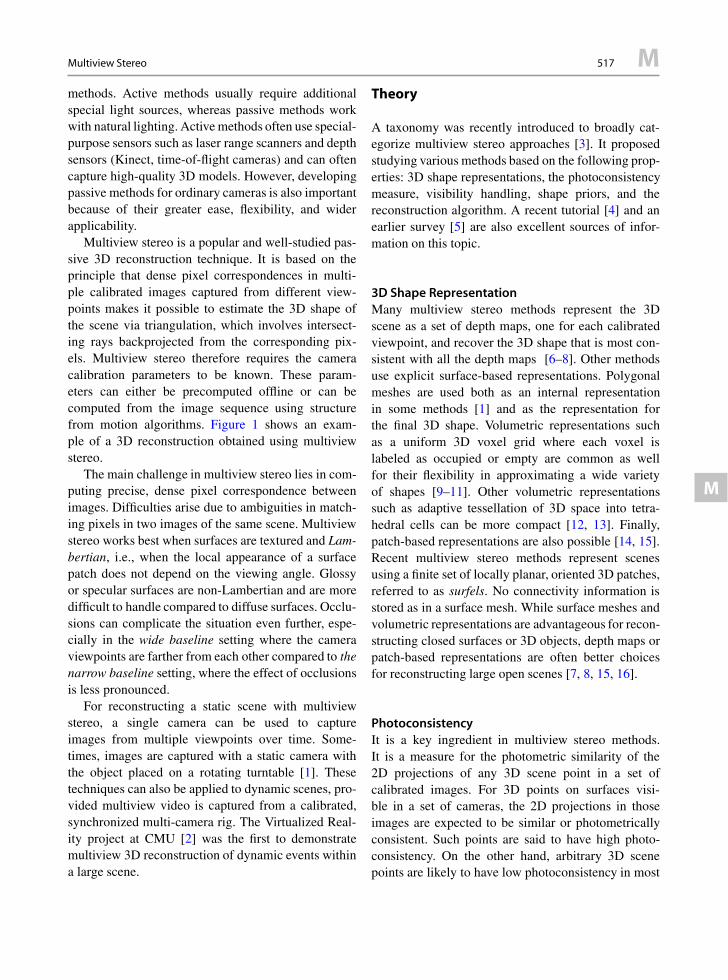
Multiview Stereo 517 M
M
methods. Active methods usually require additionalspecial light sources, whereas passive methods workwith natural lighting. Active methods often use special-purpose sensors such as laser range scanners and depthsensors (Kinect, time-of-flight cameras) and can oftencapture high-quality 3D models. However, developingpassive methods for ordinary cameras is also importantbecause of their greater ease, flexibility, and widerapplicability.
Multiview stereo is a popular and well-studied pas-sive 3D reconstruction technique. It is based on theprinciple that dense pixel correspondences in multi-ple calibrated images captured from different view-points makes it possible to estimate the 3D shape ofthe scene via triangulation, which involves intersect-ing rays backprojected from the corresponding pix-els. Multiview stereo therefore requires the cameracalibration parameters to be known. These param-eters can either be precomputed offline or can becomputed from the image sequence using structurefrom motion algorithms. Figure 1 shows an exam-ple of a 3D reconstruction obtained using multiviewstereo.
The main challenge in multiview stereo lies in com-puting precise, dense pixel correspondence betweenimages. Difficulties arise due to ambiguities in match-ing pixels in two images of the same scene. Multiviewstereo works best when surfaces are textured and Lam-bertian, i.e., when the local appearance of a surfacepatch does not depend on the viewing angle. Glossyor specular surfaces are non-Lambertian and are moredifficult to handle compared to diffuse surfaces. Occlu-sions can complicate the situation even further, espe-cially in the wide baseline setting where the cameraviewpoints are farther from each other compared to thenarrow baseline setting, where the effect of occlusionsis less pronounced.
For reconstructing a static scene with multiviewstereo, a single camera can be used to captureimages from multiple viewpoints over time. Some-times, images are captured with a static camera withthe object placed on a rotating turntable [1]. Thesetechniques can also be applied to dynamic scenes, pro-vided multiview video is captured from a calibrated,synchronized multi-camera rig. The Virtualized Real-ity project at CMU [2] was the first to demonstratemultiview 3D reconstruction of dynamic events withina large scene.
Theory
A taxonomy was recently introduced to broadly cat-egorize multiview stereo approaches [3]. It proposedstudying various methods based on the following prop-erties: 3D shape representations, the photoconsistencymeasure, visibility handling, shape priors, and thereconstruction algorithm. A recent tutorial [4] and anearlier survey [5] are also excellent sources of infor-mation on this topic.
3D Shape RepresentationMany multiview stereo methods represent the 3Dscene as a set of depth maps, one for each calibratedviewpoint, and recover the 3D shape that is most con-sistent with all the depth maps [6–8]. Other methodsuse explicit surface-based representations. Polygonalmeshes are used both as an internal representationin some methods [1] and as the representation forthe final 3D shape. Volumetric representations suchas a uniform 3D voxel grid where each voxel islabeled as occupied or empty are common as wellfor their flexibility in approximating a wide varietyof shapes [9–11]. Other volumetric representationssuch as adaptive tessellation of 3D space into tetra-hedral cells can be more compact [12, 13]. Finally,patch-based representations are also possible [14, 15].Recent multiview stereo methods represent scenesusing a finite set of locally planar, oriented 3D patches,referred to as surfels. No connectivity information isstored as in a surface mesh. While surface meshes andvolumetric representations are advantageous for recon-structing closed surfaces or 3D objects, depth maps orpatch-based representations are often better choicesfor reconstructing large open scenes [7, 8, 15, 16].
PhotoconsistencyIt is a key ingredient in multiview stereo methods.It is a measure for the photometric similarity of the2D projections of any 3D scene point in a set ofcalibrated images. For 3D points on surfaces visi-ble in a set of cameras, the 2D projections in thoseimages are expected to be similar or photometricallyconsistent. Such points are said to have high photo-consistency. On the other hand, arbitrary 3D scenepoints are likely to have low photoconsistency in most

M 518 Multiview Stereo
Multiview Stereo, Fig. 1 Images captured with a camera rig. Calibrated cameras and the final 3d model produced by a state-of-the-art multiview stereo method rendered as a triangulated mesh
Multiview Stereo, Fig. 2 (a) A pixel in a reference image andand a square patch around it. (b) Corresponding pixels and asso-ciated patches in the nearby images that lie on respective epipo-lar lines. In calibrated images, the search for correspondences
reduces to 1D, i.e., along the epipolar line. (c) A horizontalslice of the 3D cost volume is shown. It is constructed usingthe photoconsistency measure described in [10]
situations. Some earlier methods used the variance inpixel colors in images where a 3D point is visible, as ameasure of photoconsistency. However, since compar-ing individual pixels can be ambiguous, a more reliableapproach is to compare the similarity of image patchesaround the projections of a 3D point (see Fig. 2). Fornarrow baselines, it is sufficient to compare image-oriented square patches centered on pixels. However,by incorporating the geometry of the 3D patch, thematching windows can be correctly adjusted to accountfor scale differences in the images and slanted surfaces.
A pair of 2D image patches can be compared usingnormalized cross correlation (NCC) after resamplinga n D k � k 2D grid at each patch and comparingthe vector of color values denoted here as u and v,respectively:
NCC.u; v/ DPn
jD0.uj � u/:.vj � v/qPn
jD0.uj � u/2:Pn
jD0.vj � v/2
(1)
The NCC-based similarity measure lies in the range[�1,1] where a value closer to 1 indicates that thevectors are similar in appearance. Other similaritymeasures such as the sum of absolute differences(SAD), the sum of squared differences (SSD), ornonparametric measures can be used to compute pho-toconsistency as well. Unlike NCC, SAD or SSD areaffected by brightness changes in different images.
Photoconsistency Volume ComputationMany multiview stereo methods require the photocon-sistency function to be evaluated densely on a 3D voxelgrid for the volume containing the scene which is thenreferred to as the cost volume. Figure 2 shows an exam-ple. One simple way to construct this cost volume is toevaluate the photoconsistency of all 3D points (or vox-els) using a pairwise similarity measure such as NCCand then compute the mean NCC score from multiplepairs of nearby images. There also exist direct meth-ods to compute the cost volume [17] or approaches thatare better at minimizing noise in the photoconsistency

Multiview Stereo 519 M
M
estimates [10]. Being able to estimate the visibilityof a 3D point allows one to select which imagescontribute to its photoconsistency measure. A coarseapproximation of the shape such as the visual hullreconstruction obtained from silhouettes is often suf-ficient when reconstructing closed objects [1, 10, 12].However, when a large number of images are available,occlusions can also be treated as outliers and explicitvisibility reasoning is not required [10, 14].
Another general approach to construct the costvolume involves first estimating depth maps fromeach camera’s viewpoint using a state-of-the-art multi-baseline stereo matching algorithm and then mergingthem into a consistent volumetric representation. Thissort of aggregation incorporates visibility informationinduced by the independently estimated depth maps.Intuitively, this can be thought of as a way of proba-bilistically carving out the 3D volume [6, 18], an ideathat is closely related to the problem of fusion of rangeimages [19].
Plane Sweep Stereo and DepthMap FusionA class of methods referred to as plane sweep stereomethods avoid building the cost volume on a uni-form 3D grid. Instead, they sweep the scene with aset of parallel planes corresponding to the candidatedepths considered for pixels in the reference image.These planes are typically fronto parallel to the refer-ence camera, and their spacing is selected in uniformintervals with respect to their inverse depth from thecamera. Neighboring images are warped on to theseplanes using 2D homographies, and the photoconsis-tency measure is computed at each pixel for eachcandidate depth plane. Plane-sweeping strategies areoften chosen by incorporating some knowledge ofscene structure and are popular for 3D recontructionin urban scenes [7]. Their main advantage over uni-form voxel grids or other 3D tessellations lies in thefact that they represent large working volumes moreefficiently, which is important for reconstructing largeopen scenes. Plane sweep stereo can be combined withdepth map fusion which can be implemented using animage space representation [8]. Artifacts in the origi-nal depth maps are reduced in the fused depth mapsfrom which triangulated surface meshes can be directlyextracted. The fusion step works better when per-pixelconfidence estimates associated with the depth esti-mates are available.
Optimization MethodsBroadly all multiview stereo methods formulate thereconstruction task in terms of a local or global opti-mization problem. A local method such as space carv-ing [9] starts with an overestimate of the 3D scene,and uses a greedy strategy to remove voxels that arenot photoconsistent one at a time. Similarly, in fastplane sweep stereo [7], each pixel’s depth is com-puted independent of other pixels. These local meth-ods are susceptible to noise and outliers and cannoteasily reconstruct smooth geometric shapes. Part ofthe difficulty is that the 3D reconstruction task isinherently ill-posed since different 3D scenes can beconsistent with the same set of images. By assum-ing that surfaces in the scene are primarily smooth,various global optimization methods seek the optimal3D shape which maximizes both photoconsistency andsmoothness. This is achieved by formulating multiviewstereo as a global optimization problem with geometricregularization terms in the objective function or energyfunction. These are minimized either in the discrete orin the continuous setting.
Global methods for depth map estimation incor-porate image-based smoothness constraints into theformulation by designing suitable energy functionsthat encourages neighboring pixels to take on identi-cal or similar depth values. Such methods are oftenbased on a 2D Markov Random Field (MRF) frame-work for which efficient optimization algorithms havebeen developed in recent years. The MRF frameworkcan also be used for enforcing surface regularization involumetric methods on a 3D uniform grid [10] whereany binary labeling of voxels in the grid correspondsto some 3D shape. The optimal surface correspond-ing to the global minimum of the energy function canbe efficiently computed using graph cut algorithms inmany situations [1, 18]. In case of [12, 13], the min-imal surface computed using graph cuts directly pro-duces a triangulated mesh. These methods first solvea discrete optimization problem to obtain a globallyconsistent solution and then performs local refine-ment using continuous optimization to recover finerdetails in the structure [1, 12]. As an alternative, directcontinuous optimization methods based on convexrelaxations have also been developed to address dis-cretization artifacts which can occur in graph cut-basedmethods [11].
Variational methods can also be used to extract anoptimal smooth surface from the cost volume using

M 520 Multiview Stereo
multiple iterations that progressively minimize a globalobjective function. In [1], this was achieved by evolv-ing a deformable surface mesh using photoconsistencycues. However, a good initial guess for the 3D shapewas required. Methods based on level sets are moreflexible as the surface topology is allowed to changeduring the iterations. These approaches represent thesurface as the zero level set of an evolving implicitfunction [20]. The energy function is minimized bymodeling the evolution of the function using partialdifferential equations. These level-set methods havethe advantage of producing smooth surface recon-structions but have the disadvantage of being suscep-tible to local minima unless a good initialization isavailable.
Patch-Based Multiview Stereo
Another class of popular multiview stereo approachesrepresent surfaces as a set of oriented patches with-out storing any connectivity information. This makesthe representation flexibile and suitable for recon-structing both closed 3D shapes and open scenes. Awatertight surface mesh can be extracted using thePoisson surface reconstruction algorithm as a post-processing step. Patch-based methods are related toregion-growing methods as they typically start froma few seed 3D points with known depth. The algo-rithm proposed in [14] starts with a sparse structurefrom motion 3D point cloud and iteratively optimizesthe depth and normals of the oriented patches usingan NCC-based photoconsistency measure. The pixelsin the reference image are processed in a matchingscore-based priority order that ensures that confidentestimates are propagated first in the surface-growingphase. This step produces semi-dense depth mapswhich are then merged to generate a global set of ori-ented 3D patches. This method was used to perform 3Dreconstruction from Internet images of popular land-marks and showed that dense correspondences couldbe reliably computed from such large heterogenousimage collections as well.
Patch-based multiview stereo (PMVS) [15] isanother popular algorithm that also uses a seed andgrow reconstruction strategy and consists of threeimportant steps. First, seed patches are created fromsparse 2D keypoint correspondences in neighboring
overlapping views which can be matched with highconfidence. These patches are iteratively expandedusing a locally planar model to generate new patches.This is followed by a patch optimization and filter-ing step which refines the position and orientation ofthe patches and then removes noisy or outlier samplesbased on photoconsistency and visibility constraints. Apublicly available implementation of this algorithm isavailable as part of the PMVS library [15]. Recently,this library was also extended to support large-scalereconstructions from Internet collections [16].
EfficientMultiview Stereo on GPUs
Some multiview stereo methods strive for high-fidelityreconstructions and can be very computationally inten-sive especially when high-resolution images are pro-cessed [1, 14–16, 21]. The main computational bottle-neck in multiview stereo lies in the photoconsistencycomputation or computing matching cost over manypairs of windows. Typically, this can be acceleratedby orders of magnitude on massively parallel hardwareand is also perfectly suitable for the data-parallelismsupported on modern programmable graphics hard-ware (GPUs) with SIMD architectures. Many vari-ants of multiview stereo ranging from plane sweepstereo [7], depth map fusion [8] to level-sets-basedmethods [22] have been successfully ported to theGPU, and one or two orders of magnitude speeduphave been demonstrated.
Benchmarks
The Middlebury multiview stereo datasets shown inFig. 3a contain ground truth 3D models created byscanning the models using a laser stripe scanner andregistering the 3D mesh to the calibrated imagescaptured with a gantry. The benchmark has recentlybeen quite popular for evaluating multiview stereoalgorithms [3]. It uses two criteria to evaluate thereconstructions – accuracy and completeness. Themodel’s accuracy is calculated by computing the dis-tance between the points sampled on the reconstructedmodel and the nearest points on the ground truth modeland reporting the distance (in mm) such that 90% ofthe points on the reconstructed model are within thatdistance from the ground truth model. Similarly, the
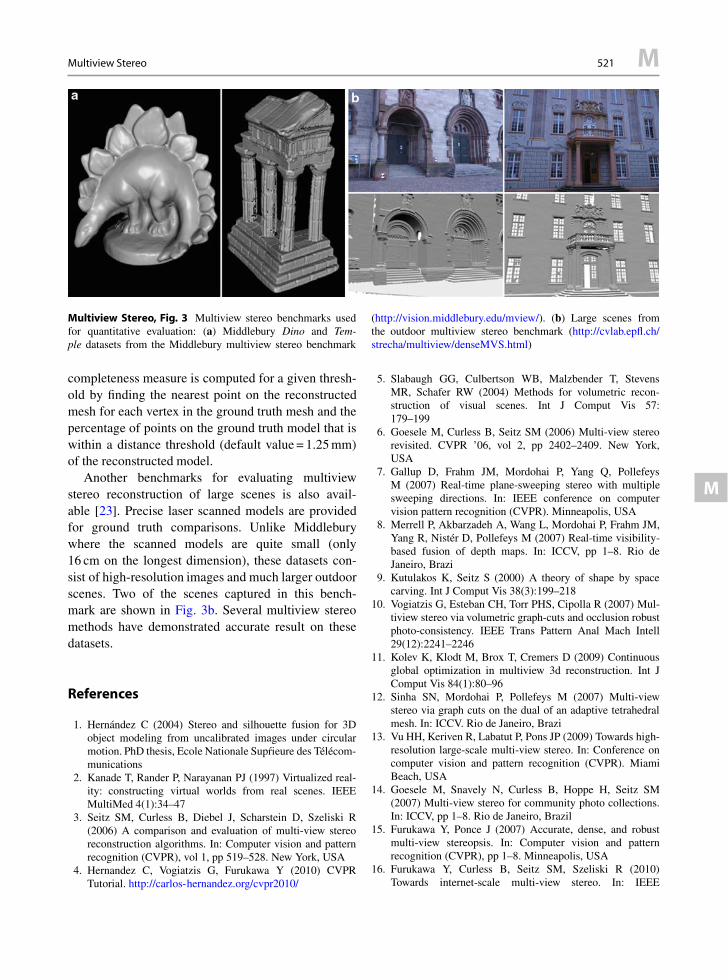
Multiview Stereo 521 M
M
Multiview Stereo, Fig. 3 Multiview stereo benchmarks usedfor quantitative evaluation: (a) Middlebury Dino and Tem-ple datasets from the Middlebury multiview stereo benchmark
(http://vision.middlebury.edu/mview/). (b) Large scenes fromthe outdoor multiview stereo benchmark (http://cvlab.epfl.ch/strecha/multiview/denseMVS.html)
completeness measure is computed for a given thresh-old by finding the nearest point on the reconstructedmesh for each vertex in the ground truth mesh and thepercentage of points on the ground truth model that iswithin a distance threshold (default value = 1.25 mm)of the reconstructed model.
Another benchmarks for evaluating multiviewstereo reconstruction of large scenes is also avail-able [23]. Precise laser scanned models are providedfor ground truth comparisons. Unlike Middleburywhere the scanned models are quite small (only16 cm on the longest dimension), these datasets con-sist of high-resolution images and much larger outdoorscenes. Two of the scenes captured in this bench-mark are shown in Fig. 3b. Several multiview stereomethods have demonstrated accurate result on thesedatasets.
References
1. Hernández C (2004) Stereo and silhouette fusion for 3Dobject modeling from uncalibrated images under circularmotion. PhD thesis, Ecole Nationale Suprieure des Télécom-munications
2. Kanade T, Rander P, Narayanan PJ (1997) Virtualized real-ity: constructing virtual worlds from real scenes. IEEEMultiMed 4(1):34–47
3. Seitz SM, Curless B, Diebel J, Scharstein D, Szeliski R(2006) A comparison and evaluation of multi-view stereoreconstruction algorithms. In: Computer vision and patternrecognition (CVPR), vol 1, pp 519–528. New York, USA
4. Hernandez C, Vogiatzis G, Furukawa Y (2010) CVPRTutorial. http://carlos-hernandez.org/cvpr2010/
5. Slabaugh GG, Culbertson WB, Malzbender T, StevensMR, Schafer RW (2004) Methods for volumetric recon-struction of visual scenes. Int J Comput Vis 57:179–199
6. Goesele M, Curless B, Seitz SM (2006) Multi-view stereorevisited. CVPR ’06, vol 2, pp 2402–2409. New York,USA
7. Gallup D, Frahm JM, Mordohai P, Yang Q, PollefeysM (2007) Real-time plane-sweeping stereo with multiplesweeping directions. In: IEEE conference on computervision pattern recognition (CVPR). Minneapolis, USA
8. Merrell P, Akbarzadeh A, Wang L, Mordohai P, Frahm JM,Yang R, Nistér D, Pollefeys M (2007) Real-time visibility-based fusion of depth maps. In: ICCV, pp 1–8. Rio deJaneiro, Brazi
9. Kutulakos K, Seitz S (2000) A theory of shape by spacecarving. Int J Comput Vis 38(3):199–218
10. Vogiatzis G, Esteban CH, Torr PHS, Cipolla R (2007) Mul-tiview stereo via volumetric graph-cuts and occlusion robustphoto-consistency. IEEE Trans Pattern Anal Mach Intell29(12):2241–2246
11. Kolev K, Klodt M, Brox T, Cremers D (2009) Continuousglobal optimization in multiview 3d reconstruction. Int JComput Vis 84(1):80–96
12. Sinha SN, Mordohai P, Pollefeys M (2007) Multi-viewstereo via graph cuts on the dual of an adaptive tetrahedralmesh. In: ICCV. Rio de Janeiro, Brazi
13. Vu HH, Keriven R, Labatut P, Pons JP (2009) Towards high-resolution large-scale multi-view stereo. In: Conference oncomputer vision and pattern recognition (CVPR). MiamiBeach, USA
14. Goesele M, Snavely N, Curless B, Hoppe H, Seitz SM(2007) Multi-view stereo for community photo collections.In: ICCV, pp 1–8. Rio de Janeiro, Brazil
15. Furukawa Y, Ponce J (2007) Accurate, dense, and robustmulti-view stereopsis. In: Computer vision and patternrecognition (CVPR), pp 1–8. Minneapolis, USA
16. Furukawa Y, Curless B, Seitz SM, Szeliski R (2010)Towards internet-scale multi-view stereo. In: IEEE

M 522 Mutual Illumination
conference on computer vision pattern recognition (CVPR).San Francisco, USA
17. Hornung A, Kobbelt L (2006) Robust and efficient photo-consistency estimation for volumetric 3d reconstruction.ECCV’06, vol 2, pp 179–190. Graz, Austria
18. Hernández C, Vogiatzis G, Cipolla R (2007) Probabilis-tic visibility for multi-view stereo. In: IEEE conference oncomputer vision pattern recognition (CVPR). Minneapolis,USA
19. Curless B, Levoy M (1996) A volumetric method for build-ing complex models from range images. In: Proceedingsof the 23rd annual conference on computer graphics andinteractive techniques. SIGGRAPH ’96, pp 303–312. NewOrleans, USA
20. Pons JP, Keriven R, Faugeras O (2007) Multi-view stereoreconstruction and scene flow estimation with a globalimage-based matching score. Int J Comput Vis 72(2):179–193
21. Tola E, Strecha C, Fua P (2011) Efficient large-scale multi-view stereo for ultra high-resolution image sets. J Mach VisAppl 23(5):903–920
22. Labatut P, Keriven R, Pons JP (2006) Fast level set multi-view stereo on graphics hardware. In: International sympo-sium on 3D data processing visualization and transmission.Chapel Hill, USA
23. Strecha C, von Hansen W, Gool LJV, Fua P, Thoennessen U(2008) On benchmarking camera calibration and multi-viewstereo for high resolution imagery. In: IEEE conference oncomputer vision pattern recognition (CVPR). Anchorage,USA
Mutual Illumination
�Interreflections


![FOR REVIEW: IEEE TRANSACTIONS ON PATTERN ANALYSIS …tai/microns_papers/zhu_AOTpami.pdfpositives, and require more training images. As a related example, in Felzenszwalb et. al. [5]](https://img.pdfslide.us/doc/110x75/5ea3236628175635967c5651/for-review-ieee-transactions-on-pattern-analysis-taimicronspaperszhu-positives.jpg)