Robust Monocular Epipolar Flow Estimation

Koichiro Yamaguchi1,2 David McAllester 1 Raquel Urtasun1

1TTI Chicago, 2Toyota Central R&D Labs., Inc{yamaguchi, mcallester, rurtasun}@ttic.edu

Abstract

We consider the problem of computing optical flow inmonocular video taken from a moving vehicle. In this set-ting, the vast majority of image flow is due to the vehi-cle’s ego-motion. We propose to take advantage of thisfact and estimate flow along the epipolar lines of the ego-motion. Towards this goal, we derive a slanted-planeMRF model which explicitly reasons about the ordering ofplanes and their physical validity at junctions. Further-more, we present a bottom-up grouping algorithm whichproduces over-segmentations that respect flow boundaries.We demonstrate the effectiveness of our approach in thechallenging KITTI flow benchmark [11] achieving half theerror of the best competing general flow algorithm and onethird of the error of the best epipolar flow algorithm.

1. Introduction

Optical flow is an important classical problem in com-puter vision, as it can be used in support of 3D reconstruc-tion, perceptual grouping and object recognition. Here weare interested in applications to autonomous vehicles. Inthis setting, most of the flow can be explained by the vehi-cle’s ego-motion. As a consequence, once the ego-motion iscomputed, one can treat flow as a matching problem alongepipolar lines. The main difference with stereo vision re-sides in the fact that the epipolar lines radiate from a singleepipole, called the focus of expansion (FOE).

A few attempts to utilize these constraints have been pro-posed [22], mainly in the context of scene flow (i.e., whena stereo pair is available). However, so far, we have notwitnessed big performance gains by employing the epipolarconstraints. In contrast, we take advantage of recent devel-opments in stereo vision to construct robust solutions to theepipolar flow problem.

This paper has three main contributions. Our first con-tribution is to adapt slanted plane stereo models [39, 2] tothe problem of monocular epipolar flow estimation. Thisallow us to exploit global energy minimization methods inorder to alleviate problems in texture-less regions and pro-duce dense flow fields. In particular, we represent the prob-lem as one of inference in a hybrid Markov random field

(MRF), where a slanted plane represents the epipolar flowfor each segment and discrete random variables representthe boundary relations between each pair of neighboringsegments (i.e., hinge, coplanar, occlusion). The introduc-tion of these boundary variables allows the model to rea-son about ownerships of the boundary as well as to enforcephysical validity of the boundary types at junctions.

In order to produce accurate results, slanted plane MRFmodels require a good over-segmentation of the image,where the planar assumption for each superpixel is approx-imately satisfied. Towards this goal, our second contribu-tion is an efficient flow-aware segmentation algorithm in thespirit of SLIC [1], but where the segmentation energy in-volves both image and flow terms. This encourages the seg-mentation to respect both image and flow discontinuities.

The success of MRF models also depends heavily onhaving good data terms. Our last contribution is a localflow matching algorithm, inspired by the very successfulstereo algorithm semi-global block matching [20], whichcomputes very accurate semi-dense flow fields.

We demonstrate the effectiveness of our approach in thechallenging KITTI flow benchmark [11] achieving half theerror of the best competing general flow algorithm and onethird of the error of the best competing epipolar flow algo-rithm. In the remainder of the paper, we first review re-lated work and present our local epipolar flow algorithm.We then discuss our unsupervised segmentation algorithmwhich preserves epipolar flow discontinuities, and presentour slanted plane MRF formulation. We conclude with ourexperimental evaluation and a discussion about future work.

2. Related Work

Over the past few decades we have witnessed a greatimprovement in performance of flow algorithms. Currentapproaches can be roughly divided into two categories:gradient-based approaches [21, 5, 41], which are typi-cally based on the brightness constancy assumption, andmatching-based approaches [22, 14, 25], which match aregion (block) around each pixel to a set of candidate lo-cations. Gradient-based methods suffer in the presence oflarge displacements as the brightness constancy assumptiondoes not hold. Moreover, the regularization employed is

1

typically too local, yielding bad results in textureless re-gions. Matching-based methods can potentially deal withlarge displacements, but are typically computationally de-manding due to the large amount of candidates required forgood accuracy. Furthermore, they also suffer from homoge-neous regions as the matching is ambiguous.

While existing many works use a variational approachfor continuous flow optimization [21, 5, 6, 41], a numberof recent approaches have proposed discrete MRF formu-lations [26, 35, 14, 25]. However, these approaches sufferfrom the discretization trade-off between the number of la-bels and the resulting computational complexity. The prob-lem is more severe than in stereo, as instead of 1D dispar-ities, a 2D flow field has to be discretized. [14, 25] use acoarse-to-fine approach and sampling, while [26, 35] cre-ate a set of candidate flow estimates by standard continuousoptical flow algorithms.

When dealing with mostly static scenes, optical flow canbe expressed as a 3D rigid motion due to the camera mo-tion. The knowledge of this epipolar geometry has been in-troduced as a soft constraint in the energy function [36, 37]or as a hard constraint [33, 22]. In the latter, first the fun-damental matrix is calculated and the flow estimation isformulated as a 1D search by restricting a correspondingpoint to lie on the epipolar line. While a soft constraint canyield less errors in independently moving objects, hard con-straints can reduce computational complexity and achieverobust estimation of flow in stationary objects if the funda-mental matrix is accurately estimated. In this paper we takethe latter approach and adapt the highly successful slanted-plane MRF approach to stereo vision for the problem ofepipolar flow estimation. As demonstrated by our experi-ments, this results in very significant performance gains.

3. Semi-global Block Matching for Flow

In this section we extend the popular stereo algorithm,semi-global block matching [20] to tackle the epipolar flowproblem. In particular, we first convert the estimation froma 2D matching problem to a 1D search along the epipolarlines, which are defined by the vehicle’s ego-motion. Wethen define parameterizations and cost functions which areappropriate for epipolar flow.

3.1. Epipolar Flow as a 1D Search Problem

The first step of our algorithm consists on estimating thefundamental matrix that defines the set of epipolar lines.Towards this goal, we simply match SIFT keypoints [28] inthe two consecutive images, and estimate the fundamentalmatrix F using RANSAC and the 8-point algorithm [15].We then estimate the parameters of the flow that is due tocamera rotation, and pose the flow problem as a 1D searchalong the translational flow component.

Image plane at time t

C

C’

o

o’

P

p

p’l’(p)

v

Image plane at time t + 1

Rotated image planeat time t

p+uw(p)

C

C’

o’

P

p’l’(p)

v

Image plane at time t + 1

o’l’(p)

Figure 1. Epipolar flow geometry.

More formally, let w = (wx, wy, wz) and v =(vx, vy, vz) be the camera rotation and translation from timet to time t + 1. Assuming that the scene is static, the flowvector u = (ux, uy) for a pixel p = (x, y) in the image attime t is given by

u = uw(p) + uv(p, Zp), (1)

where uw(p),uv(p, Zp) are the components of the flowdue to the camera rotation and translation, respectively, andZp is the depth of pixel p.

Assuming that the camera rotation between two imagesis small, uw(p) can be expressed as follows [27],

uw(p) =

(fwy − wz y +

wy

f x2 − wx

f xy

−fwx + wzx+wy

f xy −wx

f y2

)where f is the focal length of the camera and x = x −cx, y = y − cy , with (cx, cy) the principal point. Thus, wecan write uw(p) as a 5-parameter model.

uw(p) = uw(p;a) =

(a1 − a3y + a4x

2 + a5xya2 + a3x+ a4xy + a5y

2

)An additional constraint that we can exploit to estimate

the rotational component of the flow is given by the fact thatuv(p, Zp) is parallel to the epipolar line passing though thatpoint at time t+1. This epipolar line is given by `′(p) = Fpwith p representing p in homogeneous coordinates. Thus,as uv(p, Zp) being parallel to the epipolar line `′(p) im-plies that p + uw(p) must be on `′(p), we can impose that

`′(p)>(p + uw(p)) = 0 (2)

with uw(p) representing uw(p) in homogeneous coordi-nates. We can then estimate the parameters of the rotationalflow, a = (a1, ..., a5), by minimizing the sum for all pixelsof the left hand side of Eq. (2). Once this is done, we onlyneed to estimate the flow in the direction of the epipolarlines. This is a 1D computation which is not only computa-tionally attractive, but also results in more accurate match-ing, as it imposes a strong regularization.

3.2. Semi-global Block Matching for Flow

We now discuss how we can adapt the semi-global blockmatching stereo algorithm (SGM) [20] to estimate the trans-lational component of flow. SGM works in three steps:

p+uw(p)

o’

o’p’

f at time t

P

Rp

Zp

vz

r

r’

C

C’v f!'

Rotated image planeImage plane at time t + 1

!'

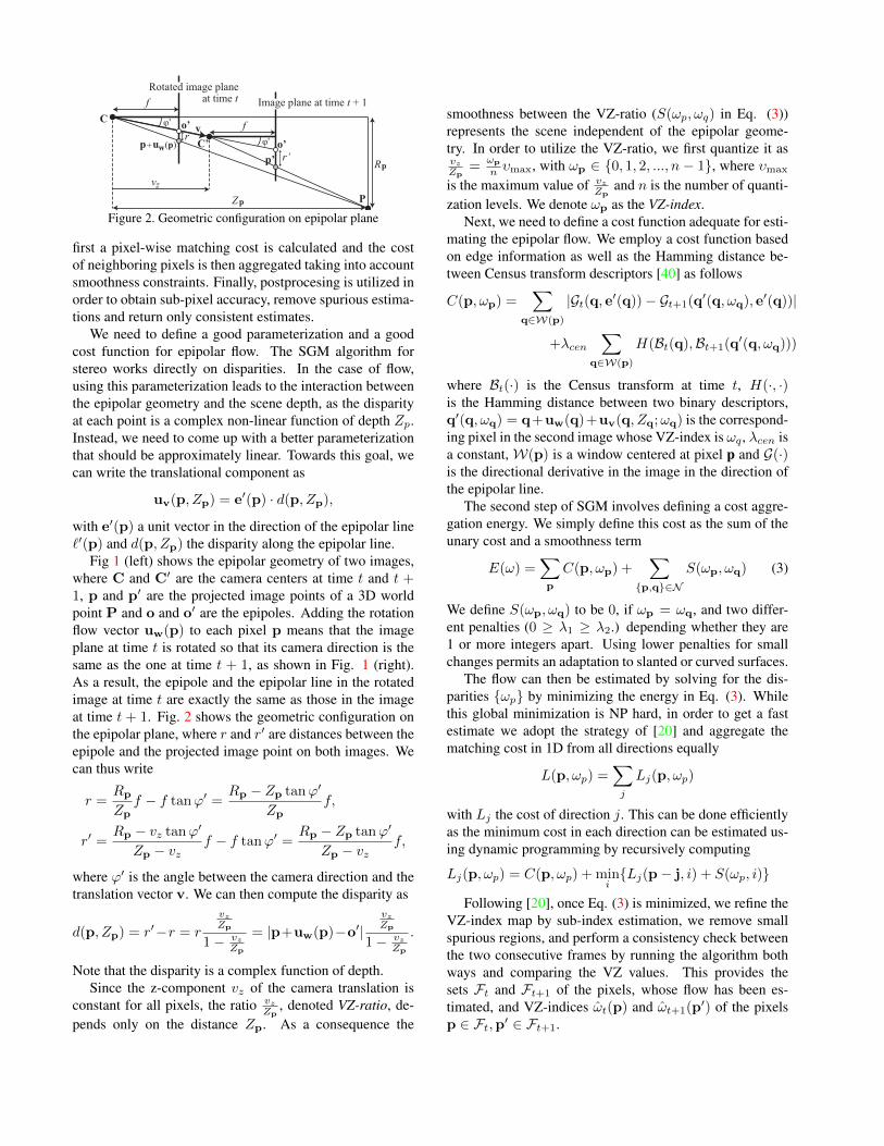
Figure 2. Geometric configuration on epipolar plane

first a pixel-wise matching cost is calculated and the costof neighboring pixels is then aggregated taking into accountsmoothness constraints. Finally, postprocesing is utilized inorder to obtain sub-pixel accuracy, remove spurious estima-tions and return only consistent estimates.

We need to define a good parameterization and a goodcost function for epipolar flow. The SGM algorithm forstereo works directly on disparities. In the case of flow,using this parameterization leads to the interaction betweenthe epipolar geometry and the scene depth, as the disparityat each point is a complex non-linear function of depth Zp.Instead, we need to come up with a better parameterizationthat should be approximately linear. Towards this goal, wecan write the translational component as

uv(p, Zp) = e′(p) · d(p, Zp),

with e′(p) a unit vector in the direction of the epipolar line`′(p) and d(p, Zp) the disparity along the epipolar line.

Fig 1 (left) shows the epipolar geometry of two images,where C and C′ are the camera centers at time t and t +1, p and p′ are the projected image points of a 3D worldpoint P and o and o′ are the epipoles. Adding the rotationflow vector uw(p) to each pixel p means that the imageplane at time t is rotated so that its camera direction is thesame as the one at time t + 1, as shown in Fig. 1 (right).As a result, the epipole and the epipolar line in the rotatedimage at time t are exactly the same as those in the imageat time t + 1. Fig. 2 shows the geometric configuration onthe epipolar plane, where r and r′ are distances between theepipole and the projected image point on both images. Wecan thus write

r =Rp

Zpf − f tanϕ′ =

Rp − Zp tanϕ′

Zpf,

r′ =Rp − vz tanϕ′

Zp − vzf − f tanϕ′ =

Rp − Zp tanϕ′

Zp − vzf,

where ϕ′ is the angle between the camera direction and thetranslation vector v. We can then compute the disparity as

d(p, Zp) = r′−r = r

vzZp

1− vzZp

= |p+uw(p)−o′|vzZp

1− vzZp

.

Note that the disparity is a complex function of depth.Since the z-component vz of the camera translation is

constant for all pixels, the ratio vzZp

, denoted VZ-ratio, de-pends only on the distance Zp. As a consequence the

smoothness between the VZ-ratio (S(ωp, ωq) in Eq. (3))represents the scene independent of the epipolar geome-try. In order to utilize the VZ-ratio, we first quantize it asvzZp

=ωp

n υmax, with ωp ∈ {0, 1, 2, ..., n − 1}, where υmax

is the maximum value of vzZp

and n is the number of quanti-zation levels. We denote ωp as the VZ-index.

Next, we need to define a cost function adequate for esti-mating the epipolar flow. We employ a cost function basedon edge information as well as the Hamming distance be-tween Census transform descriptors [40] as follows

C(p, ωp) =∑

q∈W(p)

|Gt(q, e′(q))− Gt+1(q′(q, ωq), e′(q))|

+λcen∑

q∈W(p)

H(Bt(q),Bt+1(q′(q, ωq)))

where Bt(·) is the Census transform at time t, H(·, ·)is the Hamming distance between two binary descriptors,q′(q, ωq) = q+uw(q)+uv(q, Zq;ωq) is the correspond-ing pixel in the second image whose VZ-index is ωq , λcen isa constant,W(p) is a window centered at pixel p and G(·)is the directional derivative in the image in the direction ofthe epipolar line.

The second step of SGM involves defining a cost aggre-gation energy. We simply define this cost as the sum of theunary cost and a smoothness term

E(ω) =∑p

C(p, ωp) +∑

{p,q}∈N

S(ωp, ωq) (3)

We define S(ωp, ωq) to be 0, if ωp = ωq, and two differ-ent penalties (0 ≥ λ1 ≥ λ2.) depending whether they are1 or more integers apart. Using lower penalties for smallchanges permits an adaptation to slanted or curved surfaces.

The flow can then be estimated by solving for the dis-parities {ωp} by minimizing the energy in Eq. (3). Whilethis global minimization is NP hard, in order to get a fastestimate we adopt the strategy of [20] and aggregate thematching cost in 1D from all directions equally

L(p, ωp) =∑j

Lj(p, ωp)

with Lj the cost of direction j. This can be done efficientlyas the minimum cost in each direction can be estimated us-ing dynamic programming by recursively computing

Lj(p, ωp) = C(p, ωp) + mini{Lj(p− j, i) + S(ωp, i)}

Following [20], once Eq. (3) is minimized, we refine theVZ-index map by sub-index estimation, we remove smallspurious regions, and perform a consistency check betweenthe two consecutive frames by running the algorithm bothways and comparing the VZ values. This provides thesets Ft and Ft+1 of the pixels, whose flow has been es-timated, and VZ-indices ωt(p) and ωt+1(p′) of the pixelsp ∈ Ft,p′ ∈ Ft+1.

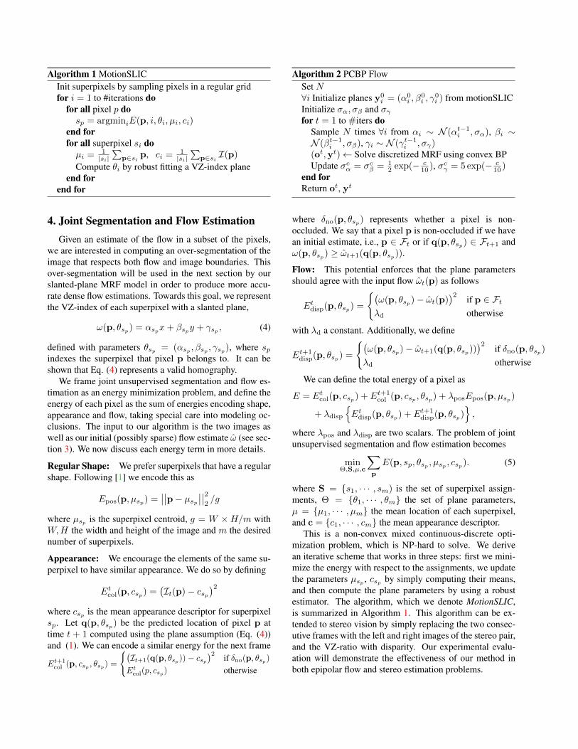
Algorithm 1 MotionSLICInit superpixels by sampling pixels in a regular gridfor i = 1 to #iterations do

for all pixel p dosp = argminiE(p, i, θi, µi, ci)

end forfor all superpixel si doµi = 1

|si|∑

p∈si p, ci = 1|si|∑

p∈si I(p)

Compute θi by robust fitting a VZ-index planeend for

end for

4. Joint Segmentation and Flow EstimationGiven an estimate of the flow in a subset of the pixels,

we are interested in computing an over-segmentation of theimage that respects both flow and image boundaries. Thisover-segmentation will be used in the next section by ourslanted-plane MRF model in order to produce more accu-rate dense flow estimations. Towards this goal, we representthe VZ-index of each superpixel with a slanted plane,

ω(p, θsp) = αspx+ βspy + γsp , (4)

defined with parameters θsp = (αsp , βsp , γsp), where spindexes the superpixel that pixel p belongs to. It can beshown that Eq. (4) represents a valid homography.

We frame joint unsupervised segmentation and flow es-timation as an energy minimization problem, and define theenergy of each pixel as the sum of energies encoding shape,appearance and flow, taking special care into modeling oc-clusions. The input to our algorithm is the two images aswell as our initial (possibly sparse) flow estimate ω (see sec-tion 3). We now discuss each energy term in more details.

Regular Shape: We prefer superpixels that have a regularshape. Following [1] we encode this as

Epos(p, µsp) =∣∣∣∣p− µsp ∣∣∣∣22 /g

where µsp is the superpixel centroid, g = W ×H/m withW,H the width and height of the image and m the desirednumber of superpixels.

Appearance: We encourage the elements of the same su-perpixel to have similar appearance. We do so by defining

Etcol(p, csp) =(It(p)− csp

)2where csp is the mean appearance descriptor for superpixelsp. Let q(p, θsp) be the predicted location of pixel p attime t + 1 computed using the plane assumption (Eq. (4))and (1). We can encode a similar energy for the next frame

Et+1col (p, csp , θsp) =

{(It+1(q(p, θsp))− csp

)2if δno(p, θsp)

Etcol(p, csp) otherwise

Algorithm 2 PCBP FlowSet N∀i Initialize planes y0

i = (α0i , β

0i , γ

0i ) from motionSLIC

Initialize σα, σβ and σγfor t = 1 to #iters do

Sample N times ∀i from αi ∼ N (αt−1i , σα), βi ∼

N (βt−1i , σβ), γi ∼ N (γt−1

i , σγ)(ot,yt)← Solve discretized MRF using convex BPUpdate σcα = σcβ = 1

2 exp(− c10 ), σcγ = 5 exp(− c

10 )end forReturn ot, yt

where δno(p, θsp) represents whether a pixel is non-occluded. We say that a pixel p is non-occluded if we havean initial estimate, i.e., p ∈ Ft or if q(p, θsp) ∈ Ft+1 andω(p, θsp) ≥ ωt+1(q(p, θsp)).

Flow: This potential enforces that the plane parametersshould agree with the input flow ωt(p) as follows

Etdisp(p, θsp) =

{(ω(p, θsp)− ωt(p)

)2if p ∈ Ft

λd otherwise

with λd a constant. Additionally, we define

Et+1disp(p, θsp) =

{(ω(p, θsp)− ωt+1(q(p, θsp))

)2if δno(p, θsp)

λd otherwise

We can define the total energy of a pixel as

E = Etcol(p, csp) + Et+1col (p, csp , θsp) + λposEpos(p, µsp)

+ λdisp

{Etdisp(p, θsp) + Et+1

disp(p, θsp)},

where λpos and λdisp are two scalars. The problem of jointunsupervised segmentation and flow estimation becomes

minΘ,S,µ,c

∑p

E(p, sp, θsp , µsp , csp). (5)

where S = {s1, · · · , sm) is the set of superpixel assign-ments, Θ = {θ1, · · · , θm} the set of plane parameters,µ = {µ1, · · · , µm} the mean location of each superpixel,and c = {c1, · · · , cm} the mean appearance descriptor.

This is a non-convex mixed continuous-discrete opti-mization problem, which is NP-hard to solve. We derivean iterative scheme that works in three steps: first we mini-mize the energy with respect to the assignments, we updatethe parameters µsp , csp by simply computing their means,and then compute the plane parameters by using a robustestimator. The algorithm, which we denote MotionSLIC,is summarized in Algorithm 1. This algorithm can be ex-tended to stereo vision by simply replacing the two consec-utive frames with the left and right images of the stereo pair,and the VZ-ratio with disparity. Our experimental evalu-ation will demonstrate the effectiveness of our method inboth epipolar flow and stereo estimation problems.

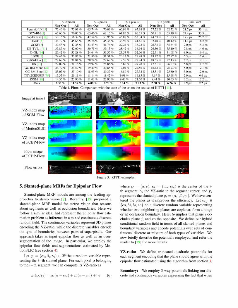
> 2 pixels > 3 pixels > 4 pixels > 5 pixels End-PointNon-Occ All Non-Occ All Non-Occ All Non-Occ All Non-Occ All

Pyramid-LK [3] 72.46 % 75.91 % 65.74 % 70.09 % 60.99 % 65.98 % 57.22 % 62.72 % 21.7 px 33.1 pxOCV-BM [4] 65.60 % 70.03 % 63.46 % 68.16 % 61.85 % 66.75 % 60.41 % 65.49 % 24.4 px 33.3 px

PolyExpand [10] 50.16 % 56.39 % 47.54 % 53.95 % 45.88 % 52.34 % 44.53 % 51.03 % 17.2 px 25.2 pxHAOF [5] 38.19 % 45.68 % 35.76 % 45.36 % 33.98 % 41.61 % 32.48 % 40.12 % 11.1 px 18.2 pxGCSF [7] 39.53 % 47.25 % 33.23 % 41.74 % 29.24 % 38.23 % 26.33 % 35.64 % 7.0 px 15.3 px

DB-TV-L1 [41] 33.87 % 42.00 % 30.75 % 39.13 % 28.42 % 36.94 % 26.50 % 35.10 % 7.8 px 14.6 pxC+NL [34] 26.42 % 35.28 % 24.64 % 33.35 % 23.53 % 32.06 % 22.71 % 31.08 % 9.0 px 16.4 pxLDOF [6] 24.43 % 33.87 % 21.86 % 31.31 % 20.13 % 29.48 % 18.72 % 27.97 % 5.5 px 12.4 px

RSRS-Flow [13] 22.68 % 31.81 % 20.74 % 29.68 % 19.55 % 28.24 % 18.65 % 27.13 % 6.2 px 12.1 pxHS [21] 22.02 % 31.18 % 19.92 % 28.86 % 18.60 % 27.28 % 17.61 % 26.07 % 5.8 px 11.7 px

GC-BM-Mono [22] 24.79 % 34.59 % 19.49 % 29.88 % 17.04 % 27.56 % 15.42 % 25.93 % 5.0 px 12.1 pxGC-BM-Bino [22] 23.07 % 33.10 % 18.93 % 29.37 % 16.80 % 27.32 % 15.31 % 25.80 % 5.0 px 12.0 px

TGV2CENSUS [38] 13.33 % 21.11 % 11.14 % 18.42 % 9.98 % 16.83 % 9.19 % 15.68 % 2.9 px 6.6 pxfSGM [18] 14.56 % 25.90 % 11.03 % 22.90 % 9.43 % 21.50 % 8.44 % 20.63 % 3.2 px 12.2 px

Ours 6.33 % 11.59 % 4.08 % 8.70 % 3.14 % 7.23 % 2.58 % 6.26 % 0.9 px 2.2 pxTable 1. Flow: Comparison with the state of the art on the test set of KITTI [11].

Image at time t

VZ-index mapof SGM-Flow

VZ-index mapof MotionSLIC

VZ-index mapof PCBP-Flow

Flow imageof PCBP-Flow

Flow errors

Figure 3. KITTI examples

5. Slanted-plane MRFs for Epipolar Flow

Slanted-plane MRF models are among the leading ap-proaches to stereo vision [2]. Recently, [39] proposed aslanted-plane MRF model for stereo vision that reasonsabout segments as well as occlusion boundaries. Here wefollow a similar idea, and represent the epipolar flow esti-mation problem as inference in a mixed continuous-discreterandom field. The continuous variables represent 3D planesencoding the VZ-ratio, while the discrete variables encodethe type of boundaries between pairs of superpixels. Ourapproach takes as input epipolar flow as well as an over-segmentation of the image. In particular, we employ theepipolar flow fields and segmentations estimated by Mo-tionSLIC (see section 4).

Let yi = (αi, βi, γi) ∈ <3 be a random variable repre-senting the i−th slanted plane. For each pixel p belongingto the i−th segment, we can compute its VZ-ratio as

ωi(p,yi) = αi(u− ciu) + βi(v − civ) + γi (6)

where p = (u, v), ci = (ciu, ciu) is the center of the i-th segment, γi the VZ-ratio in the segment center, and yirepresents the slanted plane yi = (αi, βi, γi). We have cen-tered the planes as it improves the efficiency. Let oi,j ∈{co, hi, lo, ro} be a discrete random variable representingwhether two neighboring planes are coplanar, form a hingeor an occlusion boundary. Here, lo implies that plane i oc-cludes plane j, and ro the opposite. We define our hybridconditional random field in terms of all slanted-planes andboundary variables and encode potentials over sets of con-tinuous, discrete or mixture of both types of variables. Wenow briefly describe the potentials employed, and refer thereader to [39] for more details.

VZ-ratio: We define truncated quadratic potentials foreach segment encoding that the plane should agree with theepipolar flow estimated using the algorithm from section 3.

Boundary: We employ 3-way potentials linking our dis-crete and continuous variables expressing the fact that when

> 2 pixels > 3 pixels > 4 pixels > 5 pixels End-PointNon-Occ All Non-Occ All Non-Occ All Non-Occ All Non-Occ All

Ours SGM-Flow 7.11 % 16.75 % 4.76 % 13.71 % 3.58 % 11.81 % 2.78 % 10.35 % 1.0 px 3.1 pxOurs MotionSLIC 6.53 % 13.19 % 4.39 % 10.25 % 3.34 % 8.53 % 2.59 % 7.28 % 0.9 px 2.3 pxOurs PCBP-Flow 6.11 % 10.97 % 4.08 % 8.22 % 3.08 % 6.67 % 2.38 % 5.58 % 0.9 px 1.8 px

Table 2. Importance of each step on the test set of KITTI [11].

> 2 pixels > 3 pixels > 4 pixels > 5 pixels End-PointNon-Occ All Non-Occ All Non-Occ All Non-Occ All Non-Occ All

disparity 8.41 % 19.07 % 5.66 % 16.21 % 4.26 % 14.56 % 3.33 % 13.33 % 1.2 px 5.0 pxVZ-index 7.11 % 16.75 % 4.76 % 13.71 % 3.58 % 11.81 % 2.78 % 10.35 % 1.0 px 3.1 px

Table 3. Use of VZ index vs disparity on SGM-Flow evaluated on the validation set of KITTI [11].

two neighboring planes are hinge or coplanar they shouldagree on the boundary, and when a segment occludes an-other, the boundary should be explained by the occluder.

Compatibility: We penalize occlusion boundaries thatare not supported by the data. Additionally, we define apotential that penalizes negative VZ-ratios.

Occam’s razor: We impose a regularization on the typeof occlusion boundary, where we prefer simpler explana-tions (i.e., coplanar better than hinge better than occlusion).

Junction Feasibility: We encode the physical validity ofjunctions of 3 and 4 planes. Although these potentials arehigh-order, they only involve variables with 4 states, thusthe additional complexity is not prohibitive.

Color similarity: This potential encodes the fact that weexpect segments which are coplanar to have similar colorstatistics, while the entropy is higher when the planes forman occlusion boundary or a hinge. We employ the χ-squareddistance between histograms of neighboring segments.

Computing the MAP estimate of our hybrid MRF is NP-hard. Instead, we rely on approximate algorithms basedon LP relaxations. Following [39] we make use of parti-cle convex belief propagation (PCBP) [29], a technique thatis guaranteed to converge and gradually approach the opti-mum. PCBP is an iterative algorithm that works as follows:For each continuous variable particles are sampled aroundthe current solution. These samples act as labels in a dis-cretized MRF which is solved to convergence using convexbelief propagation [16]. The current solution is then up-dated with the MAP estimate obtained on the discretizedMRF. This process is repeated for a fixed number of itera-tions. In our implementation, we use the distributed mes-sage passing algorithm of [32] to solve the discretized MRFat each iteration. Algorithm 2 depicts our PCBP-Flow al-gorithm. At each iteration, to balance the trade off betweenexploration and exploitation, we decrease the variance ofthe distribution we sample from. Following [39], we dis-cretize the continuous variables, and utilize the algorithmof [17] for learning the importance of each potential.

6. Experimental EvaluationWe perform our experiments on the challenging KITTI

dataset [11], which is composed of 194 training and 195 test

high-resolution images captured from an autonomous driv-ing platform driving around a urban environment. We use10 images for training and 184 for validation. The groundtruth is semi-dense covering approximately 30 % of the pix-els. We employ two different metrics to evaluate our ap-proach. The first one measures the average number of pix-els (non-occluded and all) whose error is bigger than a fixedthreshold. The second one reports end-point error for bothsettings. For all experiments, we employ the same param-eters which have been validated on the validation set. Weuse υmax = 0.3 and n = 256 for our discretization of theVZ-ratio. For SGM-Flow, we set λcen = 0.5, λ1 = 100,λ2 = 1600, use a window W(p) of size 5×5, and aggre-gate information over 4 paths. Unless otherwise stated, forMotionSLIC we set the number of superpixels m = 400,λpos = 4000, λdisp = 30, λd = 3, use 10 iterations and aLab vector as the mean color representation. For PCBP, weemploy the same parameter values as [39], and run infer-ence with 10 particles and 5 iterations of re-sampling.

Comparison with the state-of-the-art: We compare ourapproach to the state-of-the-art in the test set of KITTI. Asshown in Table 1, our approach significantly outperformsall approaches, yielding approximately half the error of thebest general flow algorithm, and a third of the error of thebest epipolar flow algorithm, i.e., GC-BM-Mono [22]. In-terestingly, even a scene flow approach, i.e., GC-BM-Bino[22] that unlike our approach utilizes stereo pairs results inthree times more error. Fig. 3 depicts our flow estimations.

Importance of each step: We evaluate the importance ofeach step of our pipeline. Table 2 depicts errors of ourSGM-Flow (section 3), our MotionSLIC (section 4) as wellas our PCBP-Flow (section 5) algorithms. Note that the out-put of SGM-flow is used as input for motionSLIC, and theoutput of motionSLIC is used as input to PCBP-flow. Eachstep significantly improves results.

Running Time: We evaluate the run time of our ap-proach. KITTI images have on average 1237 × 374 pix-els. SGM-Flow takes on average 5.7s per image, 1.5s forMotionSLIC and 3.5 minutes for PCBP-Flow. Thus state-of-the-art estimates can be obtained in only a few seconds,as SGM-Flow and MotionSLIC significantly outperforms

> 2 pixels > 3 pixels > 4 pixels > 5 pixels End-PointNon-Occ All Non-Occ All Non-Occ All Non-Occ All Non-Occ All

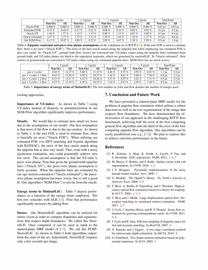
Oracle FOE 0.000 % 0.000 % 0.000 % 0.000 % 0.000 % 0.000 % 0.000 % 0.000 % 0.02 px 0.03 pxEstimated FOE 0.33 % 0.48 % 0.17 % 0.22 % 0.06 % 0.10 % 0.00 % 0.02 % 0.2 px 0.2 px

Oracle GT 1.46 % 1.77 % 1.14 % 1.33 % 0.98 % 1.12 % 0.87 % 0.98 % 0.3 px 0.4 pxOracle estimated 2.47 % 3.15 % 1.75 % 2.12 % 1.39 % 1.64 % 1.18 % 1.37 % 0.5 px 0.6 pxOur SGM-Flow 6.11 % 10.97 % 4.08 % 8.22 % 3.08 % 6.67 % 2.38 % 5.58 % 0.9 px 1.8 px

Table 4. Epipolar constraint and piece-wise planar assumptions on the validation set of KITTI [11]. If the true FOE is used to estimateflow, there is no error (“Oracle FOE”). The error of the best oracle match along the epipolar line when employing our estimated FOE isalso very small. In “Oracle GT”, ground truth flow vectors are converted into VZ-index values using the epipolar lines estimated fromground truth, and VZ-index planes are fitted to the superpixel segments, which are generated by motionSLIC. In “Oracle estimated”, flowvectors of ground truth are converted to VZ-index values using our estimated epipolar lines. SGM-Flow has no oracle access.

> 2 pixels > 3 pixels > 4 pixels > 5 pixels End-PointNon-Occ All Non-Occ All Non-Occ All Non-Occ All Non-Occ All

pos + 1-color 8.02 % 14.37 % 5.68 % 11.22 % 4.46 % 9.35 % 3.59 % 8.01 % 1.1 px 2.4 pxpos + 1-color + 1-flow 6.63 % 13.26 % 4.50 % 10.33 % 3.44 % 8.61 % 2.69 % 7.36 % 0.9 px 2.3 pxpos + 1-color + 2-flow 6.53 % 13.17 % 4.42 % 10.26 % 3.37 % 8.55 % 2.62 % 7.31 % 0.9 px 2.3 pxpos + 2-color + 2-flow 6.53 % 13.19 % 4.39 % 10.25 % 3.34 % 8.53 % 2.59 % 7.28 % 0.9 px 2.3 px

Table 5. Importance of energy terms of MotionSLIC: The first number in color and flow denotes the number of images used.

existing approaches.

Importance of VZ-index: As shown in Table 3 usingVZ-index instead of disparity as parameterization in ourSGM-Flow algorithm significantly improves performance.

Oracle: We would like to estimate how much we loosedue to the assumptions of our model. Our first assumptionis that most of the flow is due to the ego-motion. As shownin Table 4, if the true FOE is used to estimate flow, thereis basically no error (“Oracle FOE”). When utilizing ourestimated FOE (via SIFT matching and 8-point algorithmwith RANSAC), the error of the best oracle match alongthe epipolar line is also very small. Thus, even with a noisyegomotion estimation, one could potentially achieve verylow error. The second assumption is that the VZ-ratio ispiece-wise planar. Note that given the ground truth epipolarlines (“Oracle GT”), the piece-wise planar assumption isfairly accurate. When the epipolar lines are estimated byour ego-motion estimation (“Oracle estimated”), the piece-wise planar assumption becomes worse, but is still a goodfit. Our algorithm (“SGM-Flow”) is not far from the oracle.

Energy terms in MotionSLIC: Table 5 depicts perfor-mance as a function of the energy terms employed. Thefirst row coincides with SLIC [1]. Note that performancesignificantly increases by adding flow.

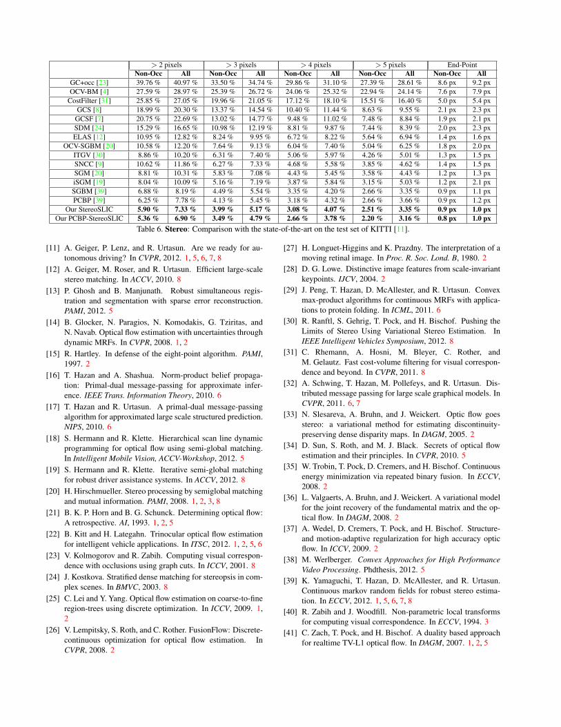
Stereo: Our MotionSLIC algorithm can be utilized forstereo vision in order to compute disparities and segmenta-tions that respect depth boundaries. We called this Stere-oSLIC. Once computed, it can be used as input to theslanted-plane MRF model of [39]. We call this PCBP-StereoSLIC. As shown in Table 6 both algorithms outper-form the state-of-the-art. Importantly, StereoSLIC requiresonly a few seconds per image.

7. Conclusion and Future Work

We have presented a slanted-plane MRF model for theproblem of epipolar flow estimation which utilizes a robustdata term as well as an over-segmentation of the image thatrespects flow boundaries. We have demonstrated the ef-fectiveness of our approach in the challenging KITTI flowbenchmark, achieving half the error of the best competinggeneral flow algorithm and one third of the error of the bestcompeting epipolar flow algorithm. Our algorithms can beeasily parallelized (see e.g., [32]). We plan to explore thisto achieve real-time performance in the future.

References[1] R. Achanta, A. Shaji, K. Smith, A. Lucchi, P. Fua, and

S. Susstrunk. SLIC superpixels. PAMI, 2012. 1, 4, 7[2] M. Bleyer, C. Rother, and P. Kohli. Surface stereo with soft

segmentation. In CVPR, 2010. 1, 5[3] J.-Y. Bouguet. Pyramidal implementation of the lucas

kanade feature tracker. Intel, 2000. 5[4] G. Bradski. The OpenCV library. Dr. Dobb’s Journal of

Software Tools, 2000. 5, 8[5] T. Brox, A. Bruhn, N. Papenberg, and J. Weickert. High ac-

curacy optical flow estimation based on a theory for warping.In ECCV, 2004. 1, 2, 5

[6] T. Brox and J. Malik. Large displacement optical flow: De-scriptor matching in variational motion estimation. PAMI,2011. 2, 5

[7] J. Cech, J. Sanchez-Riera, and R. P. Horaud. Scene flow es-timation by growing correspondence seeds. In CVPR, 2011.5, 8

[8] J. Cech and R. Sara. Efficient sampling of disparity space forfast and accurate matching. In BenCOS, 2007. 8

[9] N. Einecke and J. Eggert. A two-stage correlation methodfor stereoscopic depth estimation. In DICTA, 2010. 8

[10] G. Farneback. Two-frame motion estimation based on poly-nomial expansion. In SCIA, 2003. 5

> 2 pixels > 3 pixels > 4 pixels > 5 pixels End-PointNon-Occ All Non-Occ All Non-Occ All Non-Occ All Non-Occ All

GC+occ [23] 39.76 % 40.97 % 33.50 % 34.74 % 29.86 % 31.10 % 27.39 % 28.61 % 8.6 px 9.2 pxOCV-BM [4] 27.59 % 28.97 % 25.39 % 26.72 % 24.06 % 25.32 % 22.94 % 24.14 % 7.6 px 7.9 px

CostFilter [31] 25.85 % 27.05 % 19.96 % 21.05 % 17.12 % 18.10 % 15.51 % 16.40 % 5.0 px 5.4 pxGCS [8] 18.99 % 20.30 % 13.37 % 14.54 % 10.40 % 11.44 % 8.63 % 9.55 % 2.1 px 2.3 px

GCSF [7] 20.75 % 22.69 % 13.02 % 14.77 % 9.48 % 11.02 % 7.48 % 8.84 % 1.9 px 2.1 pxSDM [24] 15.29 % 16.65 % 10.98 % 12.19 % 8.81 % 9.87 % 7.44 % 8.39 % 2.0 px 2.3 pxELAS [12] 10.95 % 12.82 % 8.24 % 9.95 % 6.72 % 8.22 % 5.64 % 6.94 % 1.4 px 1.6 px

OCV-SGBM [20] 10.58 % 12.20 % 7.64 % 9.13 % 6.04 % 7.40 % 5.04 % 6.25 % 1.8 px 2.0 pxITGV [30] 8.86 % 10.20 % 6.31 % 7.40 % 5.06 % 5.97 % 4.26 % 5.01 % 1.3 px 1.5 pxSNCC [9] 10.62 % 11.86 % 6.27 % 7.33 % 4.68 % 5.58 % 3.85 % 4.62 % 1.4 px 1.5 pxSGM [20] 8.81 % 10.31 % 5.83 % 7.08 % 4.43 % 5.45 % 3.58 % 4.43 % 1.2 px 1.3 pxiSGM [19] 8.04 % 10.09 % 5.16 % 7.19 % 3.87 % 5.84 % 3.15 % 5.03 % 1.2 px 2.1 pxSGBM [39] 6.88 % 8.19 % 4.49 % 5.54 % 3.35 % 4.20 % 2.66 % 3.35 % 0.9 px 1.1 pxPCBP [39] 6.25 % 7.78 % 4.13 % 5.45 % 3.18 % 4.32 % 2.66 % 3.66 % 0.9 px 1.2 px

Our StereoSLIC 5.90 % 7.33 % 3.99 % 5.17 % 3.08 % 4.07 % 2.51 % 3.35 % 0.9 px 1.0 pxOur PCBP-StereoSLIC 5.36 % 6.90 % 3.49 % 4.79 % 2.66 % 3.78 % 2.20 % 3.16 % 0.8 px 1.0 px

Table 6. Stereo: Comparison with the state-of-the-art on the test set of KITTI [11].

[11] A. Geiger, P. Lenz, and R. Urtasun. Are we ready for au-tonomous driving? In CVPR, 2012. 1, 5, 6, 7, 8

[12] A. Geiger, M. Roser, and R. Urtasun. Efficient large-scalestereo matching. In ACCV, 2010. 8

[13] P. Ghosh and B. Manjunath. Robust simultaneous regis-tration and segmentation with sparse error reconstruction.PAMI, 2012. 5

[14] B. Glocker, N. Paragios, N. Komodakis, G. Tziritas, andN. Navab. Optical flow estimation with uncertainties throughdynamic MRFs. In CVPR, 2008. 1, 2

[15] R. Hartley. In defense of the eight-point algorithm. PAMI,1997. 2

[16] T. Hazan and A. Shashua. Norm-product belief propaga-tion: Primal-dual message-passing for approximate infer-ence. IEEE Trans. Information Theory, 2010. 6

[17] T. Hazan and R. Urtasun. A primal-dual message-passingalgorithm for approximated large scale structured prediction.NIPS, 2010. 6

[18] S. Hermann and R. Klette. Hierarchical scan line dynamicprogramming for optical flow using semi-global matching.In Intelligent Mobile Vision, ACCV-Workshop, 2012. 5

[19] S. Hermann and R. Klette. Iterative semi-global matchingfor robust driver assistance systems. In ACCV, 2012. 8

[20] H. Hirschmueller. Stereo processing by semiglobal matchingand mutual information. PAMI, 2008. 1, 2, 3, 8

[21] B. K. P. Horn and B. G. Schunck. Determining optical flow:A retrospective. AI, 1993. 1, 2, 5

[22] B. Kitt and H. Lategahn. Trinocular optical flow estimationfor intelligent vehicle applications. In ITSC, 2012. 1, 2, 5, 6

[23] V. Kolmogorov and R. Zabih. Computing visual correspon-dence with occlusions using graph cuts. In ICCV, 2001. 8

[24] J. Kostkova. Stratified dense matching for stereopsis in com-plex scenes. In BMVC, 2003. 8

[25] C. Lei and Y. Yang. Optical flow estimation on coarse-to-fineregion-trees using discrete optimization. In ICCV, 2009. 1,2

[26] V. Lempitsky, S. Roth, and C. Rother. FusionFlow: Discrete-continuous optimization for optical flow estimation. InCVPR, 2008. 2

[27] H. Longuet-Higgins and K. Prazdny. The interpretation of amoving retinal image. In Proc. R. Soc. Lond. B, 1980. 2

[28] D. G. Lowe. Distinctive image features from scale-invariantkeypoints. IJCV, 2004. 2

[29] J. Peng, T. Hazan, D. McAllester, and R. Urtasun. Convexmax-product algorithms for continuous MRFs with applica-tions to protein folding. In ICML, 2011. 6

[30] R. Ranftl, S. Gehrig, T. Pock, and H. Bischof. Pushing theLimits of Stereo Using Variational Stereo Estimation. InIEEE Intelligent Vehicles Symposium, 2012. 8

[31] C. Rhemann, A. Hosni, M. Bleyer, C. Rother, andM. Gelautz. Fast cost-volume filtering for visual correspon-dence and beyond. In CVPR, 2011. 8

[32] A. Schwing, T. Hazan, M. Pollefeys, and R. Urtasun. Dis-tributed message passing for large scale graphical models. InCVPR, 2011. 6, 7

[33] N. Slesareva, A. Bruhn, and J. Weickert. Optic flow goesstereo: a variational method for estimating discontinuity-preserving dense disparity maps. In DAGM, 2005. 2

[34] D. Sun, S. Roth, and M. J. Black. Secrets of optical flowestimation and their principles. In CVPR, 2010. 5

[35] W. Trobin, T. Pock, D. Cremers, and H. Bischof. Continuousenergy minimization via repeated binary fusion. In ECCV,2008. 2

[36] L. Valgaerts, A. Bruhn, and J. Weickert. A variational modelfor the joint recovery of the fundamental matrix and the op-tical flow. In DAGM, 2008. 2

[37] A. Wedel, D. Cremers, T. Pock, and H. Bischof. Structure-and motion-adaptive regularization for high accuracy opticflow. In ICCV, 2009. 2

[38] M. Werlberger. Convex Approaches for High PerformanceVideo Processing. Phdthesis, 2012. 5

[39] K. Yamaguchi, T. Hazan, D. McAllester, and R. Urtasun.Continuous markov random fields for robust stereo estima-tion. In ECCV, 2012. 1, 5, 6, 7, 8

[40] R. Zabih and J. Woodfill. Non-parametric local transformsfor computing visual correspondence. In ECCV, 1994. 3

[41] C. Zach, T. Pock, and H. Bischof. A duality based approachfor realtime TV-L1 optical flow. In DAGM, 2007. 1, 2, 5