Machinen Vision and Dig. Image Analysis 1 Prof. Heikki Kälviäinen CT50A6100 Lectures 8&9: Image Segmentation Professor Heikki Kälviäinen Machine Vision

Machinen Vision and Dig. Image Analysis

1 Prof. Heikki Kälviäinen CT50A6100

Lectures 8&9: Image Segmentation

Professor Heikki Kälviäinen

Machine Vision and Pattern Recognition LaboratoryDepartment of Information Technology

Faculty of Technology ManagementLappeenranta University of Technology (LUT)

[email protected]://www.lut.fi/~kalviai

http://www.it.lut.fi/ip/research/mvpr/


Prof. Heikki Kälviäinen CT50A6100

2

Content

• Motivation.• Detection of discontinuities.• Edge linking and boundary detection.

– Local processing.– Global processing: Hough Transform.

• Thresholding.• Region-oriented segmentation.

– Region growing. – Region splitting and merging.

• Motion-based segmentation.



3

Segmentation: Motivation

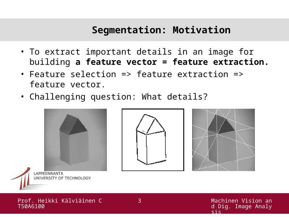
• To extract important details in an image for building a feature vector = feature extraction.

• Feature selection => feature extraction => feature vector. • Challenging question: What details?



4

Detection of discontinuities

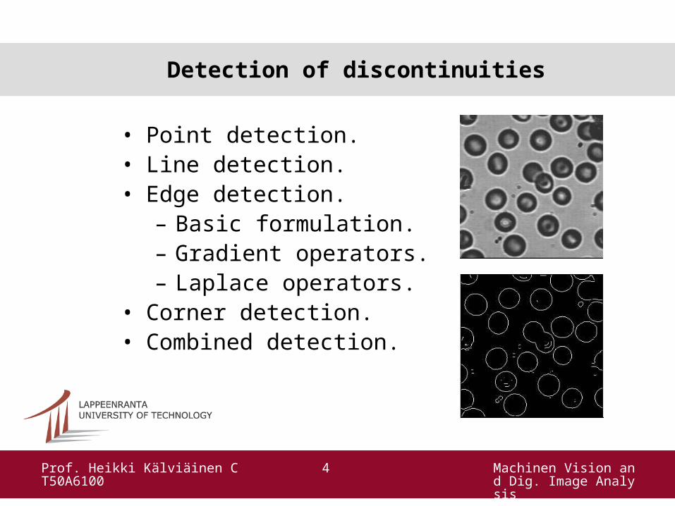
• Point detection.• Line detection.• Edge detection.

– Basic formulation.– Gradient operators.– Laplace operators.

• Corner detection.• Combined detection.



5

Point detection

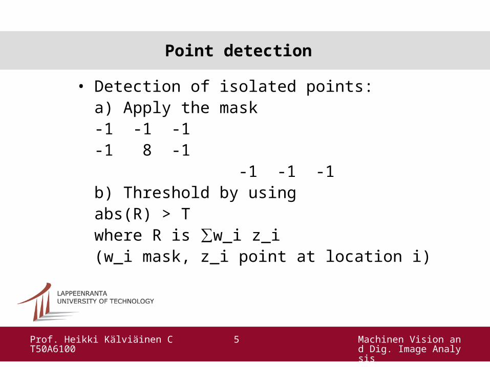
• Detection of isolated points:a) Apply the mask

-1 -1 -1-1 8 -1

-1 -1 -1b) Threshold by using

abs(R) > T where R is ∑w_i z_i (w_i mask, z_i point at location i)



6

Line detection

• Directed filters (lines of one pixel thick):

Horizontal +45 °-1 -1 -1 -1 -1 2

2 2 2 -1 2 -1 -1 -1 -1 2 -1 -1

Vertical -45 ° -1 2 -1 2 -1 -1 -1 2 -1 -1 2 -1 -1 2 -1 -1 -1 2



7

Edge detection

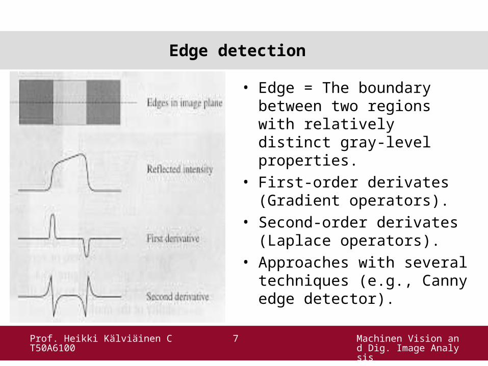
• Edge = The boundary between two regions with relatively distinct gray-level properties.

• First-order derivates (Gradient operators).

• Second-order derivates (Laplace operators).

• Approaches with several techniques (e.g., Canny edge detector).



8

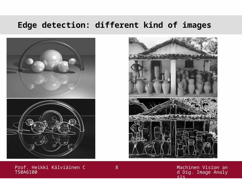
Edge detection: different kind of images



9

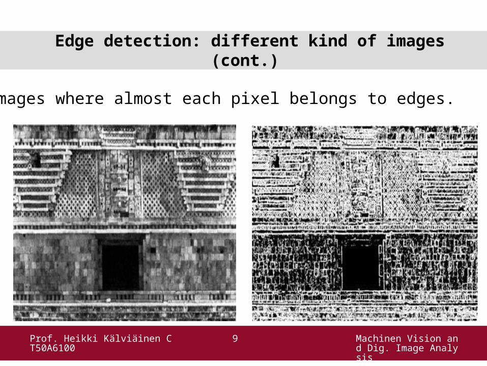
Edge detection: different kind of images (cont.)

Images where almost each pixel belongs to edges.



10

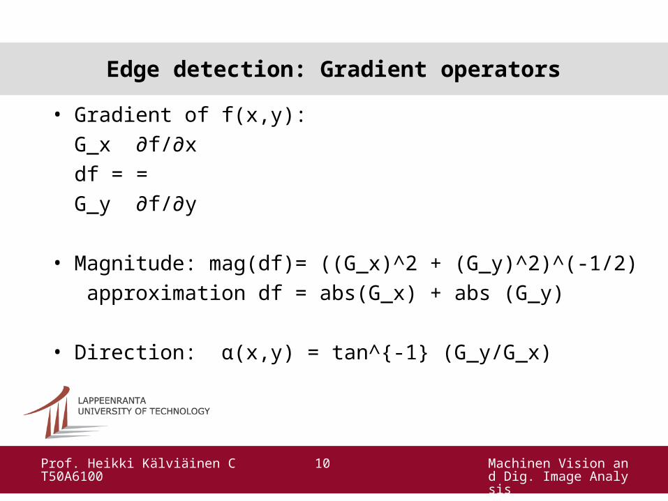
Edge detection: Gradient operators

• Gradient of f(x,y):

G_x ∂f/∂x

df = =

G_y ∂f/∂y

• Magnitude: mag(df)= ((G_x)^2 + (G_y)^2)^(-1/2)

approximation df = abs(G_x) + abs (G_y)

• Direction: α(x,y) = tan^{-1} (G_y/G_x)



11

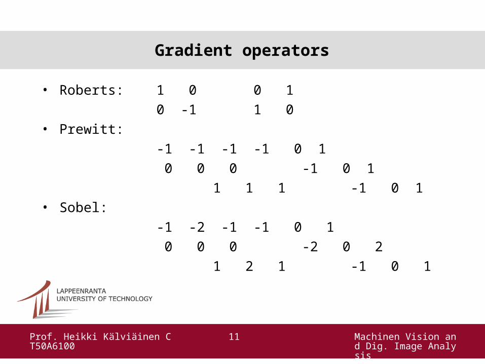
Gradient operators

• Roberts: 1 0 0 1

0 -1 1 0• Prewitt:

-1 -1 -1 -1 0 1

0 0 0 -1 0 1

1 1 1 -1 0 1• Sobel:

-1 -2 -1 -1 0 1

0 0 0 -2 0 2

1 2 1 -1 0 1



12

Edge detection: 3x3 Prewitt operator

• Horizontal mask (left top). • Vertical mask (left bottom). • Sum of the two masks (right middle).



13

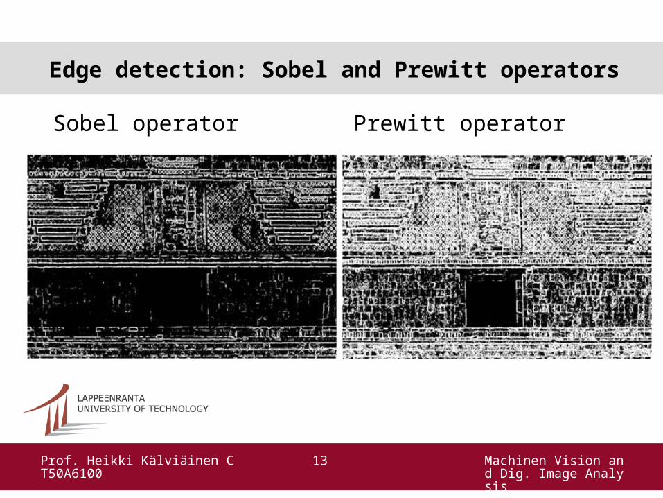
Edge detection: Sobel and Prewitt operators

Sobel operator Prewitt operator



14

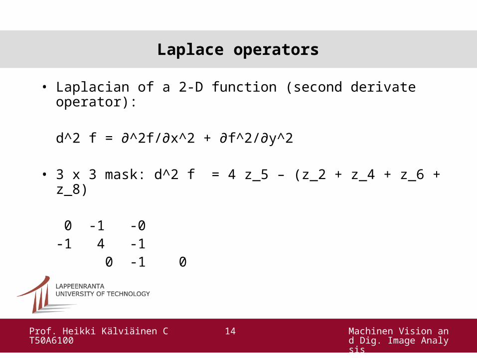
Laplace operators

• Laplacian of a 2-D function (second derivate operator):

d^2 f = ∂^2f/∂x^2 + ∂f^2/∂y^2

• 3 x 3 mask: d^2 f = 4 z_5 – (z_2 + z_4 + z_6 + z_8)

0 -1 -0 -1 4 -1

0 -1 0



15

Laplace operators (cont.)

• Sensitive to noise. • Finding the location of edges using its zero-crossing property. • Convolve an image with the Laplacian of 2-D Gaussian function of

the form

h(x,y) = exp(-(x^2+y^2)/2σ^2)

where σ is the standard deviation. • Let r^2 = x^2 + y^2:

d^2 h = (r^2-σ^2)/σ^4 exp(-(r^2)/2σ^2)

zero-crossings at r = ±σ



16

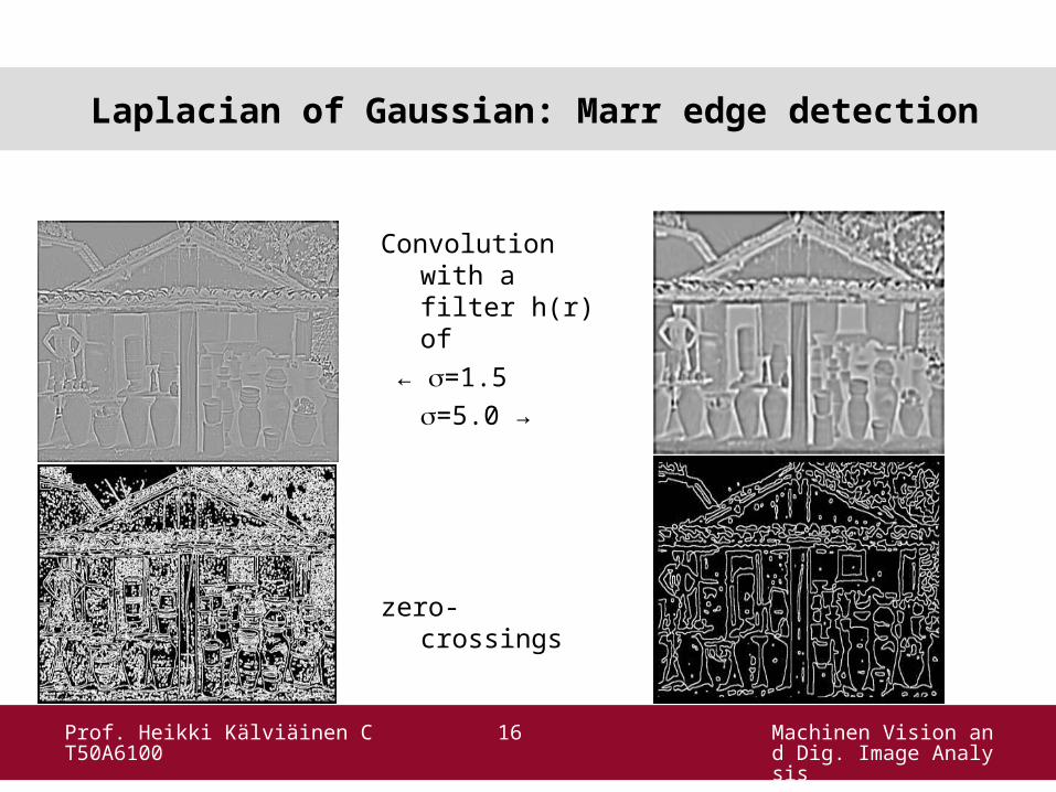
Laplacian of Gaussian: Marr edge detection

Convolution with a filter h(r) of

← =1.5

=5.0 →

zero-crossings



17

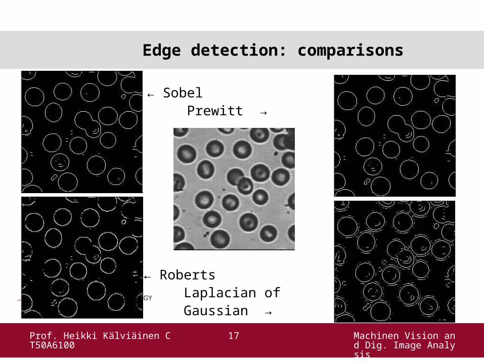
Edge detection: comparisons

← Sobel Prewitt →

← Roberts Laplacian of Gaussian →



18

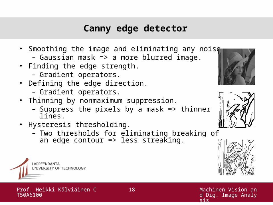
Canny edge detector

• Smoothing the image and eliminating any noise. – Gaussian mask => a more blurred image.

• Finding the edge strength.– Gradient operators.

• Defining the edge direction.– Gradient operators.

• Thinning by nonmaximum suppression. – Suppress the pixels by a mask => thinner lines.

• Hysteresis thresholding.– Two thresholds for eliminating breaking of an edge

contour => less streaking.



19

Harris corner detector

• Corners are usually very suitable interest points. • As the intersection of two edges or as the region of two different

strong edge orientations. • Based on the local auto-correlation function of a signal C(x,y)

which measures the local changes of the signal with patches shifted by a small amount in different directions.

• Corner response H(x) defined as a function of C(x,y). • Interest points can be found as local maxima in the corner

response.



20

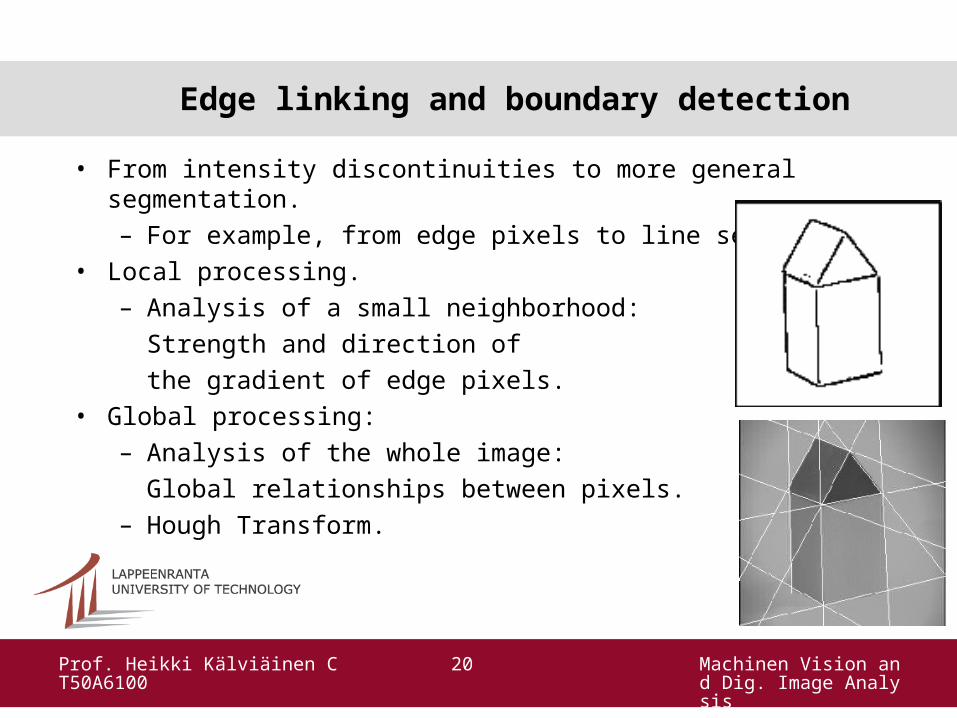
Edge linking and boundary detection

• From intensity discontinuities to more general segmentation. – For example, from edge pixels to line segments.

• Local processing.– Analysis of a small neighborhood:

Strength and direction of

the gradient of edge pixels.• Global processing:

– Analysis of the whole image:

Global relationships between pixels. – Hough Transform.



21

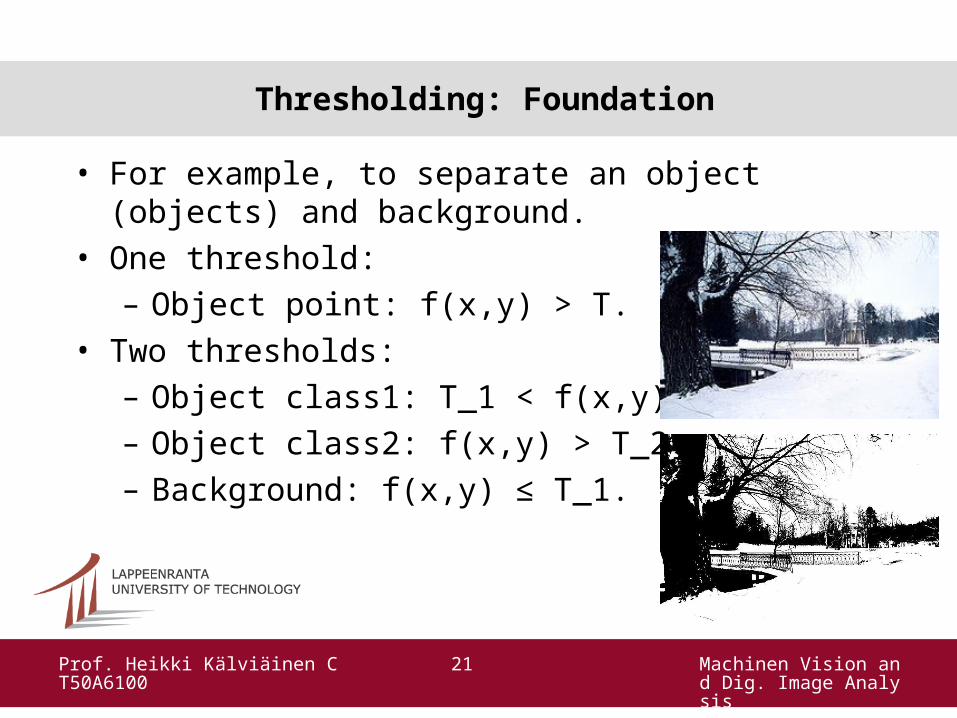
Thresholding: Foundation

• For example, to separate an object (objects) and background.

• One threshold: – Object point: f(x,y) > T.

• Two thresholds: – Object class1: T_1 < f(x,y) < T_2.– Object class2: f(x,y) > T_2. – Background: f(x,y) ≤ T_1.



22

Thresholding: Foundation (cont.)

• Operation.

T = T[x, y, p(x,y), f(x,y)]

where

f(x,y) is the gray-level point of (x,y)

p(x,y) denotes some local property of this point (e.g., the average gray-level of a neighborhood centered on (x,y))

• A thresholded image is g(x,y) is defined as

g(x,y) = 1 if f(x,y) > T

0 if f(x,y) ≤ T.



23

Thresholding: Role of illumination

• An image f(x,y) is a product of a reflectance component r(x,y) and an illumination component i(x,y).

• Original image => suitable histogram to thresholding

Original image + illumination changes =>

unsuitable histogram to thresholding• Ready for illumination changes?



24

Thresholding: Global and optimal

• How:– Simple global thresholding: just select T manually.– Optimal thresholding: optimally by probability densities (Gaussian)

p(z) = exp(-(z-μ)^2 / (2σ^2)) / (√(2πσ)) where μ is the mean value and σ is the standard deviation

• Mixture probability density of two classes: p(z) = P_1 p_1(z) + P_2 p_2(z)where P_1 and P_2 are the a priori probabilities P_1 + P_2 = 1.



25

Thresholding: Global and optimal (cont.)

• The threshold value for which error is minimal

P_1 p_1(T) = P_2 p_2(T)

• If σ = σ_1 = σ_2 by solving the equation, T is obtained as

T = (μ_1 + μ_2)/2 + (σ^2/(μ_1 - μ_2)) ln(P_2/P_1)

• If P_1=P_2 the optimal threshold is the average of the means.



26

Thresholding: Global and optimal (cont.)

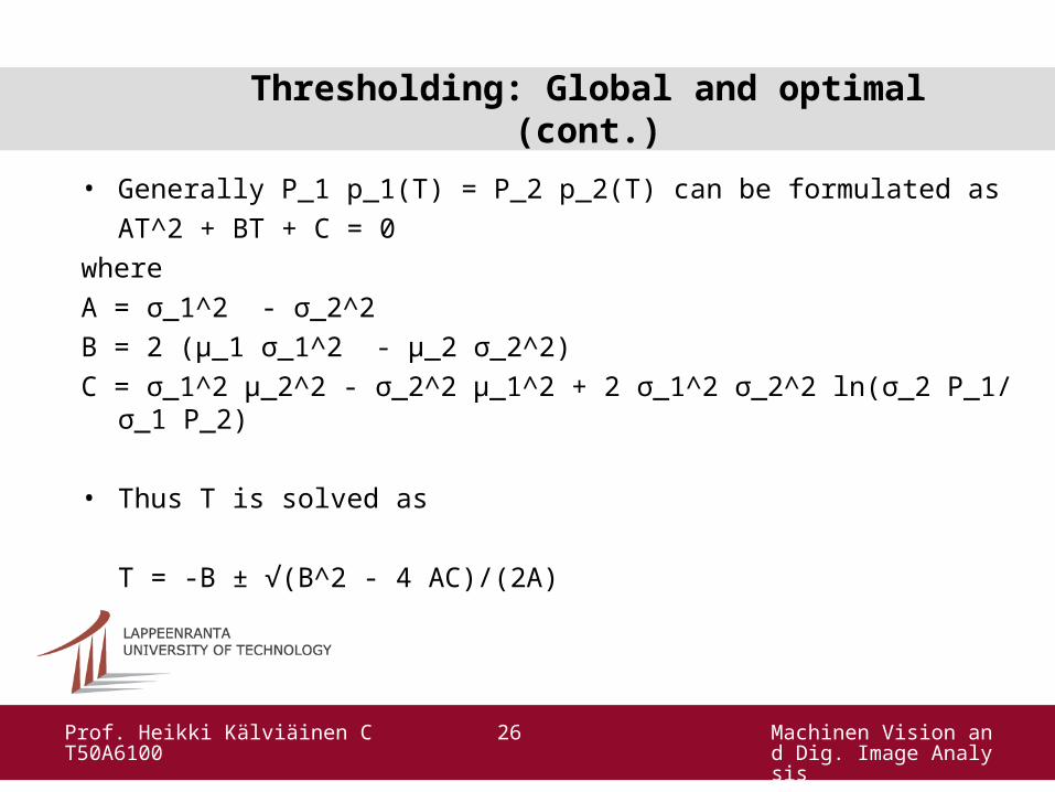
• Generally P_1 p_1(T) = P_2 p_2(T) can be formulated as

AT^2 + BT + C = 0

where

A = σ_1^2 - σ_2^2

B = 2 (μ_1 σ_1^2 - μ_2 σ_2^2)

C = σ_1^2 μ_2^2 - σ_2^2 μ_1^2 + 2 σ_1^2 σ_2^2 ln(σ_2 P_1/ σ_1 P_2)

• Thus T is solved as

T = -B ± √(B^2 - 4 AC)/(2A)



27

Thresholding: Categories of methods

Mehmet Sezgin, Bulent Sankur, Survey over image thresholding

techniques and quantitative performance evaluation, Journal of

Electronic Imaging, Vol. 13, No. 1, 2004, pp. 146-165: • Histogram shape-based methods. • Clustering-based methods. • Entropy-based methods. • Object attribute-based methods. • Spatial methods.• Local methods.



28

Region-oriented segmentation

• Region growing. – Bottom-up. – Pixel by pixel.– Pixel aggregation.

• Region splitting and merging.– Top-down.– Subdivisions of the image.– Split and merge.



29

Region growing

• Pixel aggregation: start with a set of seed points and from these grow regions by appending to each seed point those neighboring pixels that have similar properties (such as gray level, texture, color).

• Which seed points? • Similar properties? Should the criterion be

constant or change as a function of current pixels.



30

Region splitting and merging

• Subdivide an image initially into a set of arbitrary, disjointed regions and then merge and/or split the regions in an attempt to satisfy given conditions.

• Method using a logical predicate P(R) over the points in set R (similar values or not):1. Split into four disjointed quadrants any region R_i

where P(R_i) = FALSE.2. Merge any adjacent regions R_j and R_k for which

P(R_j U R_K) = TRUE.3. Stop when no further merging or splitting is possible.



31

Summary

Image acquisition => digital image

↓

Preprocessing => better image

↓

Segmentation => features for classification/clustering.

Documents

Machinen Vision and Dig. Image Analysis 1 Prof. Heikki Kälviäinen CT50A6100 Lectures 8&9: Image Segmentation Professor Heikki Kälviäinen Machine Vision