Embed Size (px)
Citation preview

Machine LearningSourangshu Bhattacharya
Algorithm for SVM training
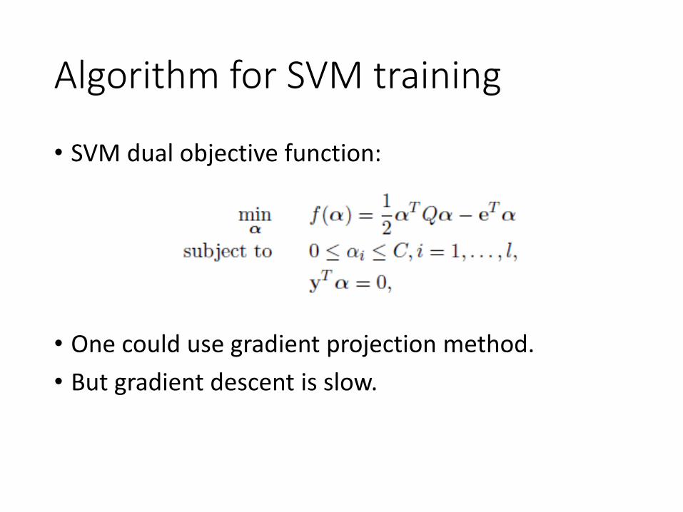
• SVM dual objective function:
• One could use gradient projection method.
• But gradient descent is slow.
Algorithm for SVM training
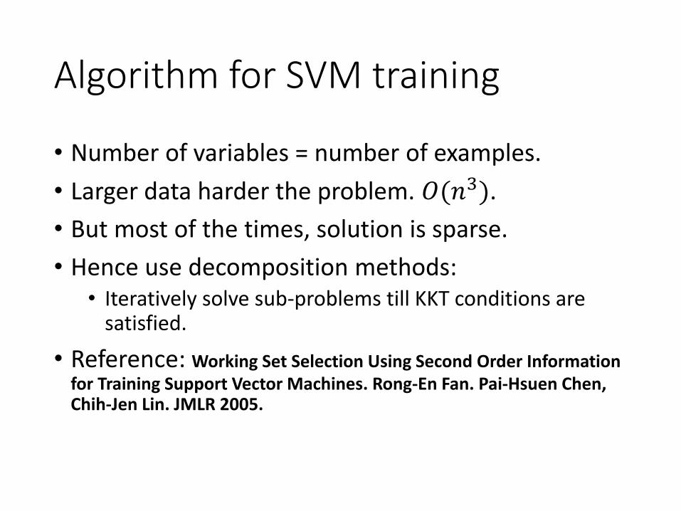
• Number of variables = number of examples.
• Larger data harder the problem. 𝑂(𝑛3).
• But most of the times, solution is sparse.
• Hence use decomposition methods:• Iteratively solve sub-problems till KKT conditions are
satisfied.
• Reference: Working Set Selection Using Second Order Information for Training Support Vector Machines. Rong-En Fan. Pai-Hsuen Chen, Chih-Jen Lin. JMLR 2005.
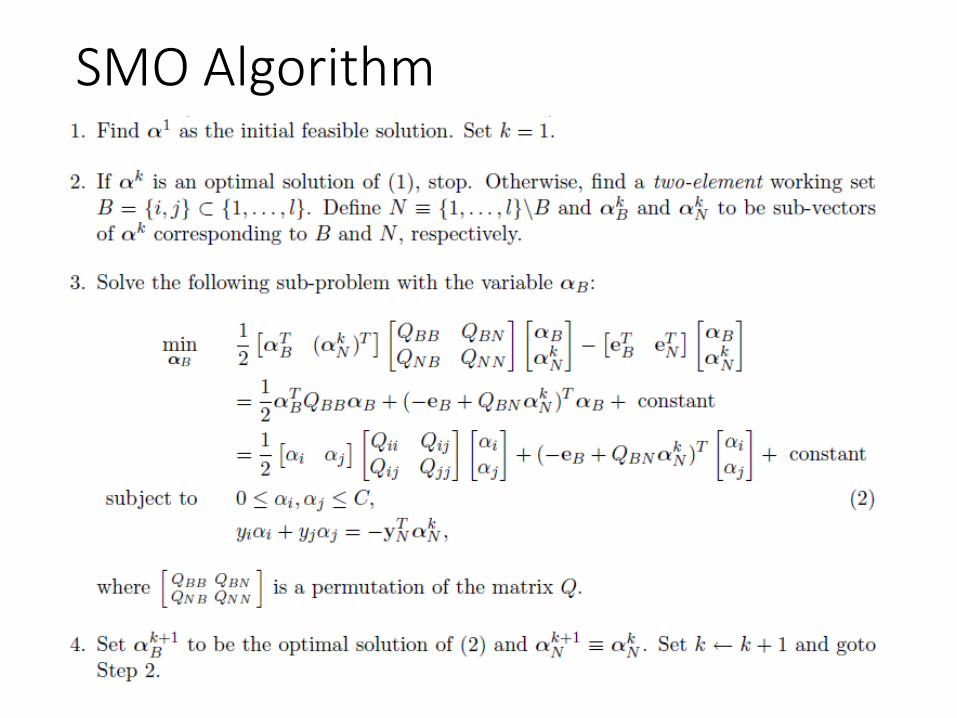
SMO Algorithm
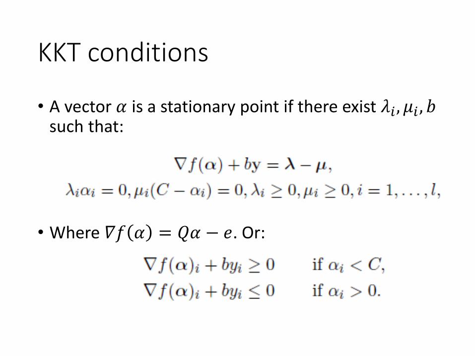
KKT conditions
• A vector 𝛼 is a stationary point if there exist 𝜆𝑖 , 𝜇𝑖 , 𝑏such that:
• Where 𝛻𝑓 𝛼 = 𝑄𝛼 − 𝑒. Or:
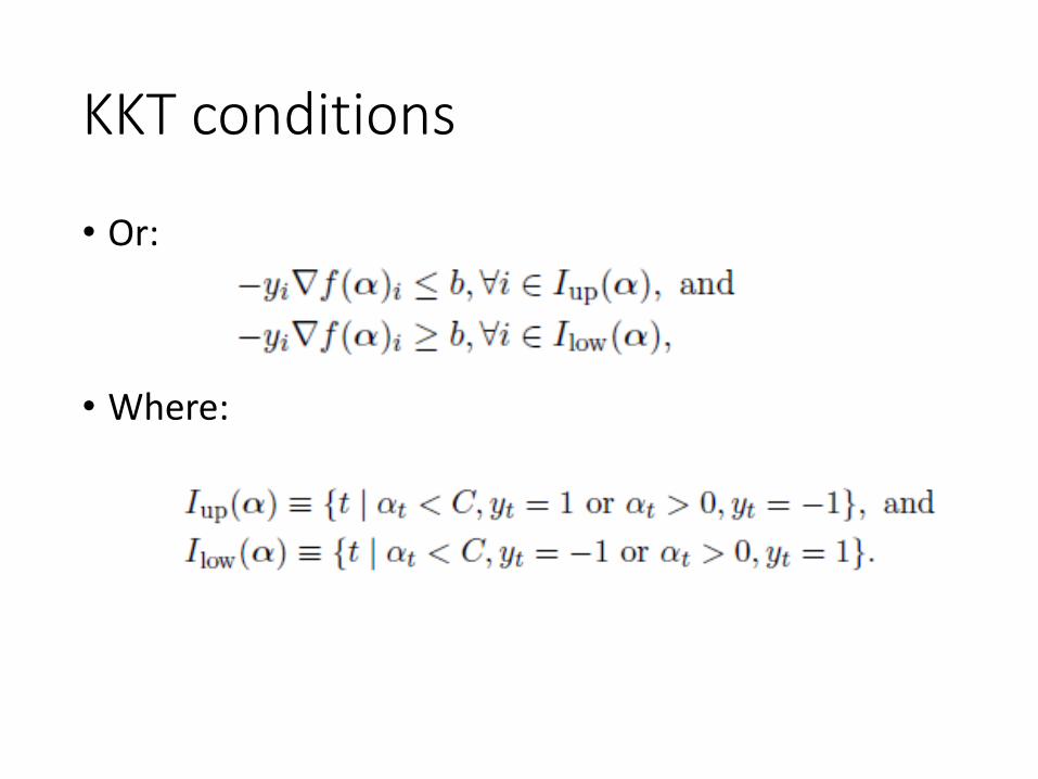
KKT conditions
• Or:
• Where:
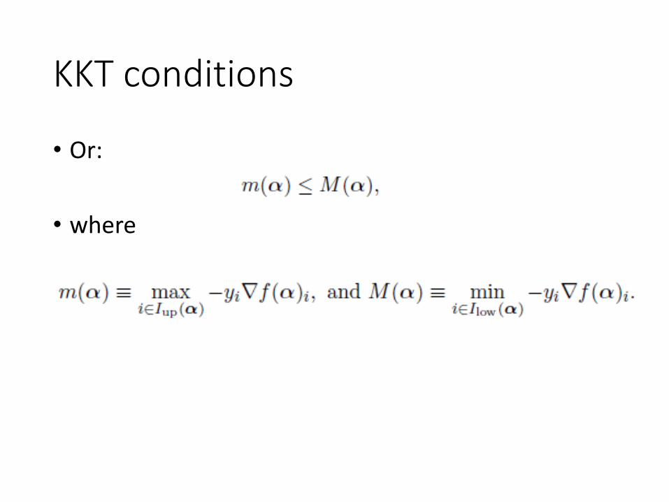
KKT conditions
• Or:
• where
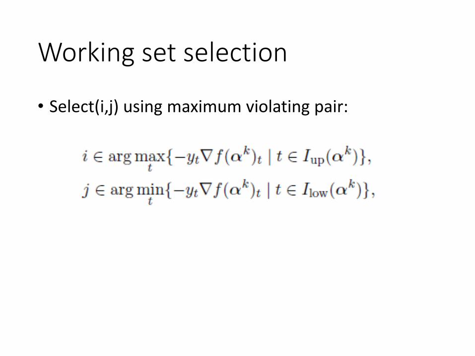
Working set selection
• Select(i,j) using maximum violating pair:

Online Learning
• Traditional machine learning assumption is that all the data points are available in the beginning.
• May not be the case:• Internet portal does not have all the data.
• A “working” model is required even when there is not enough data.
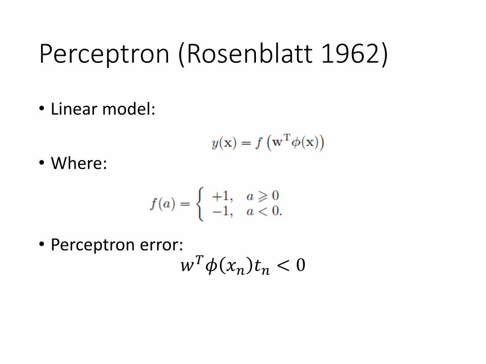
Perceptron (Rosenblatt 1962)
• Linear model:
• Where:
• Perceptron error:𝑤𝑇𝜙 𝑥𝑛 𝑡𝑛 < 0
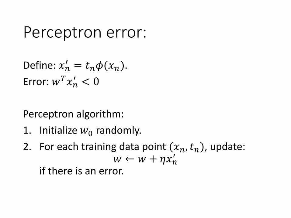
Perceptron error:
Define: 𝑥𝑛′ = 𝑡𝑛𝜙(𝑥𝑛).
Error: 𝑤𝑇𝑥𝑛′ < 0
Perceptron algorithm:
1. Initialize 𝑤0 randomly.
2. For each training data point (𝑥𝑛, 𝑡𝑛), update:𝑤 ← 𝑤 + 𝜂𝑥𝑛
′
if there is an error.
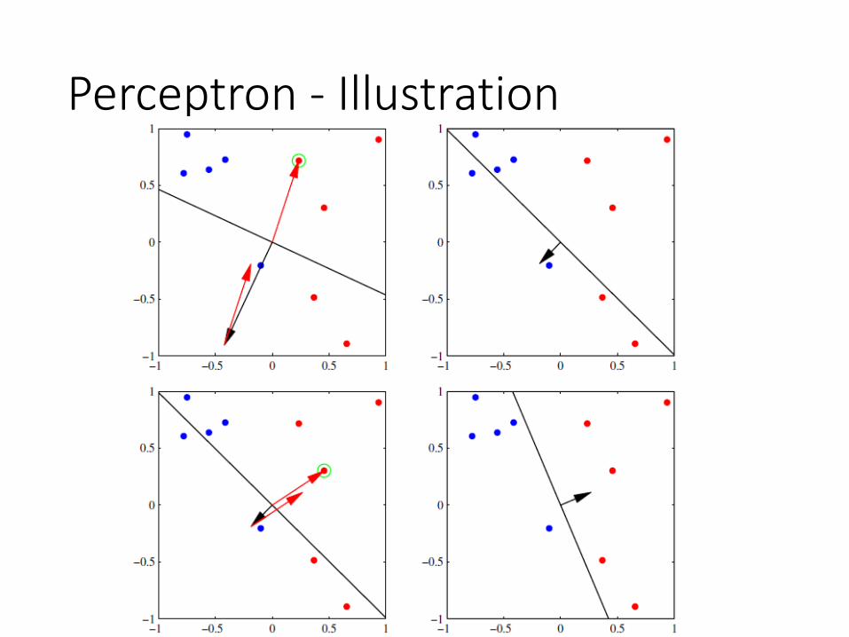
Perceptron - Illustration

Perceptron convergence theorem
• Given a linearly separable dataset 𝐷 ={(𝑥𝑛, 𝑡𝑛)|𝑛 = 1…𝑁} such that w∗T𝑥𝑛
′ > 0, 𝑛 =1…𝑁, for some 𝑤∗. The perceptron learning algorithm converges in a finite updates.
• Reference:http://www.cems.uvm.edu/~rsnapp/teaching/cs295ml/notes/perceptron.pdf
Perceptron convergence proof
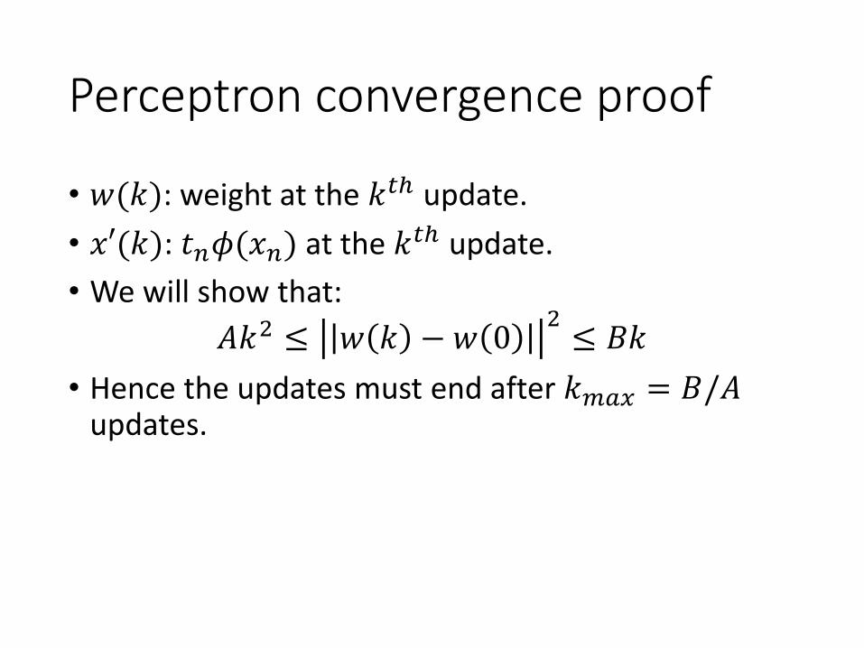
• 𝑤(𝑘): weight at the 𝑘𝑡ℎ update.
• 𝑥′(𝑘): 𝑡𝑛𝜙(𝑥𝑛) at the 𝑘𝑡ℎ update.
• We will show that:
𝐴𝑘2 ≤ 𝑤 𝑘 − 𝑤 02≤ 𝐵𝑘
• Hence the updates must end after 𝑘𝑚𝑎𝑥 = 𝐵/𝐴updates.
Perceptron convergence proof
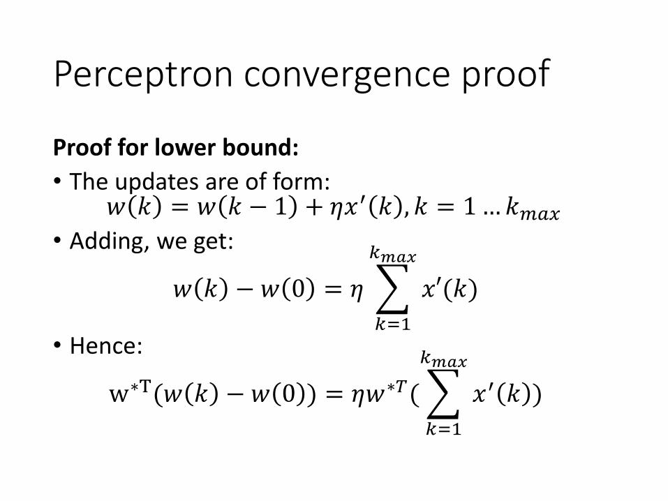
Proof for lower bound:
• The updates are of form:𝑤 𝑘 = 𝑤 𝑘 − 1 + 𝜂𝑥′ 𝑘 , 𝑘 = 1…𝑘𝑚𝑎𝑥
• Adding, we get:
𝑤 𝑘 − 𝑤 0 = 𝜂
𝑘=1
𝑘𝑚𝑎𝑥
𝑥′(𝑘)
• Hence:
w∗T(𝑤 𝑘 − 𝑤 0 ) = 𝜂𝑤∗𝑇(
𝑘=1
𝑘𝑚𝑎𝑥
𝑥′ 𝑘 )
Perceptron convergence proof
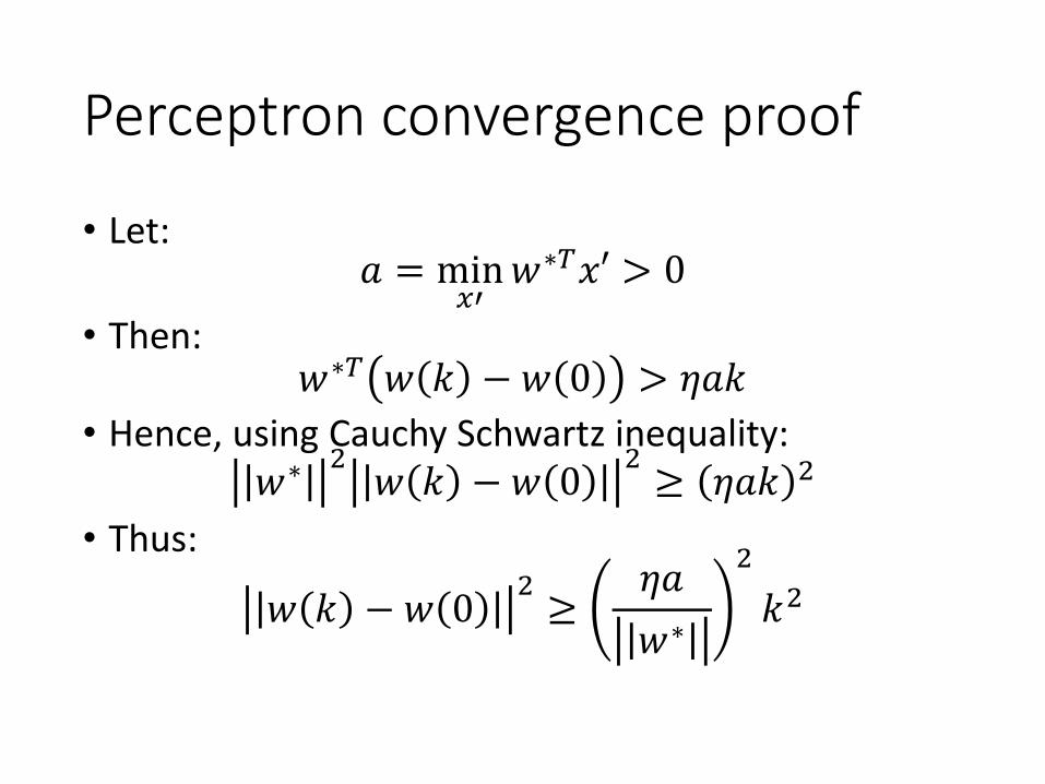
• Let:𝑎 = min
𝑥′𝑤∗𝑇𝑥′ > 0
• Then:𝑤∗𝑇 𝑤 𝑘 − 𝑤 0 > 𝜂𝑎𝑘
• Hence, using Cauchy Schwartz inequality:𝑤∗2𝑤 𝑘 − 𝑤 0
2≥ 𝜂𝑎𝑘 2
• Thus:
𝑤 𝑘 − 𝑤 02≥𝜂𝑎
𝑤∗
2
𝑘2
Perceptron convergence proof
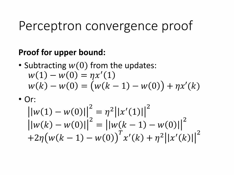
Proof for upper bound:
• Subtracting 𝑤(0) from the updates:𝑤 1 − 𝑤 0 = 𝜂𝑥′ 1𝑤 𝑘 − 𝑤 0 = 𝑤 𝑘 − 1 − 𝑤 0 + 𝜂𝑥′(𝑘)
• Or:
𝑤 1 − 𝑤 02= 𝜂2 𝑥′ 1
2
𝑤 𝑘 − 𝑤 02= 𝑤 𝑘 − 1 − 𝑤 0
2
+2𝜂 𝑤 𝑘 − 1 − 𝑤 0𝑇𝑥′ 𝑘 + 𝜂2 𝑥′ 𝑘
2
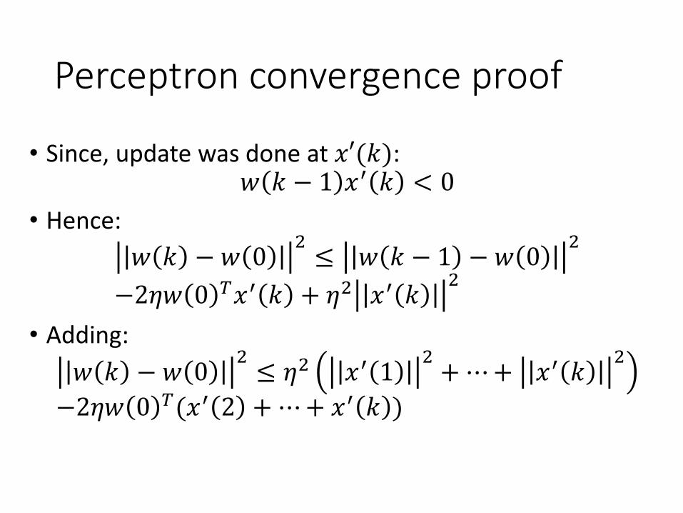
Perceptron convergence proof
• Since, update was done at 𝑥′(𝑘):𝑤 𝑘 − 1 𝑥′ 𝑘 < 0
• Hence:
𝑤 𝑘 − 𝑤 02≤ 𝑤 𝑘 − 1 − 𝑤 0
2
−2𝜂𝑤 0 𝑇𝑥′ 𝑘 + 𝜂2 𝑥′ 𝑘2
• Adding:
𝑤 𝑘 − 𝑤 02≤ 𝜂2 𝑥′ 1
2+⋯+ 𝑥′ 𝑘
2
−2𝜂𝑤 0 𝑇(𝑥′ 2 +⋯+ 𝑥′ 𝑘 )
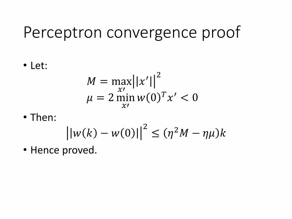
Perceptron convergence proof
• Let:
𝑀 = max𝑥′𝑥′2
𝜇 = 2min𝑥′𝑤 0 𝑇𝑥′ < 0
• Then:
𝑤 𝑘 − 𝑤 02≤ 𝜂2𝑀 − 𝜂𝜇 𝑘
• Hence proved.
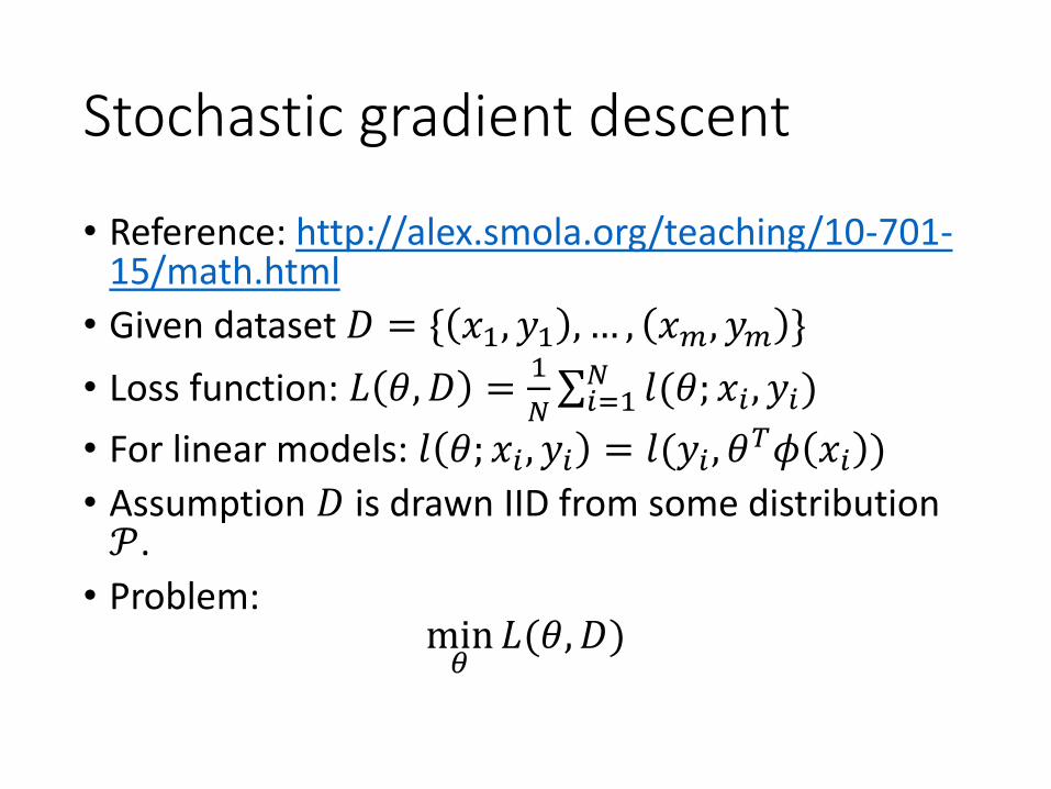
Stochastic gradient descent
• Reference: http://alex.smola.org/teaching/10-701-15/math.html
• Given dataset 𝐷 = { 𝑥1, 𝑦1 , … , 𝑥𝑚, 𝑦𝑚 }
• Loss function: 𝐿 𝜃, 𝐷 =1
𝑁 𝑖=1𝑁 𝑙(𝜃; 𝑥𝑖 , 𝑦𝑖)
• For linear models: 𝑙 𝜃; 𝑥𝑖 , 𝑦𝑖 = 𝑙(𝑦𝑖 , 𝜃𝑇𝜙 𝑥𝑖 )
• Assumption 𝐷 is drawn IID from some distribution 𝒫.
• Problem:min𝜃𝐿(𝜃, 𝐷)
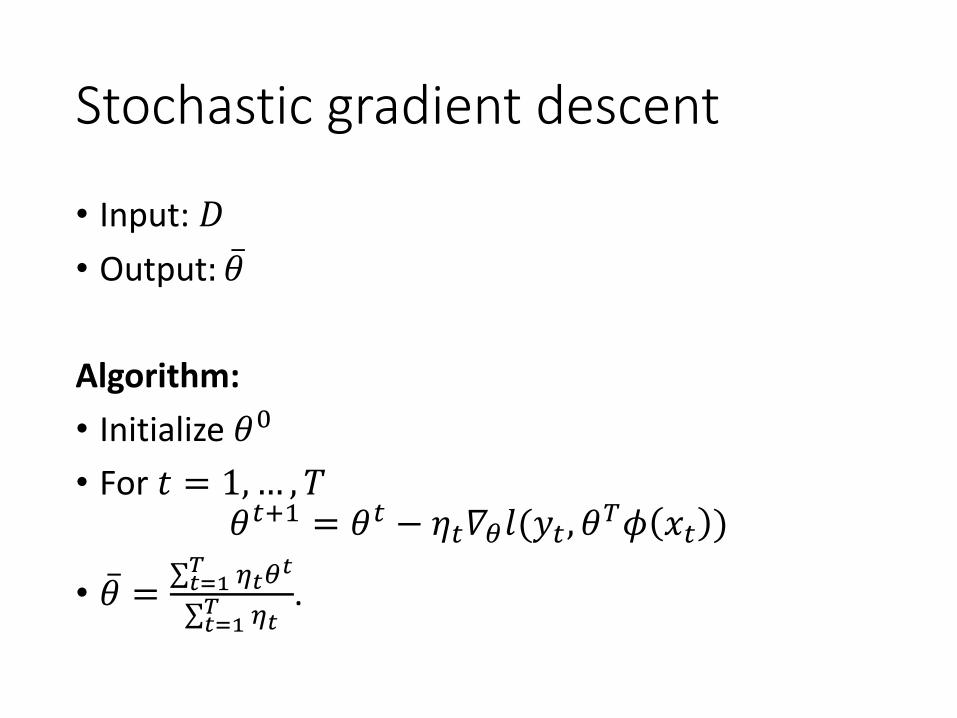
Stochastic gradient descent
• Input: 𝐷
• Output: 𝜃
Algorithm:
• Initialize 𝜃0
• For 𝑡 = 1,… , 𝑇𝜃𝑡+1 = 𝜃𝑡 − 𝜂𝑡𝛻𝜃𝑙(𝑦𝑡 , 𝜃
𝑇𝜙 𝑥𝑡 )
• 𝜃 = 𝑡=1𝑇 𝜂𝑡𝜃
𝑡
𝑡=1𝑇 𝜂𝑡
.
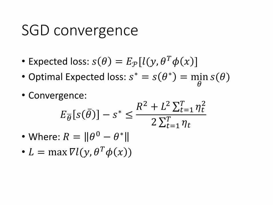
SGD convergence
• Expected loss: 𝑠 𝜃 = 𝐸𝒫[𝑙(𝑦, 𝜃𝑇𝜙 𝑥 ]
• Optimal Expected loss: 𝑠∗ = 𝑠 𝜃∗ = min𝜃𝑠(𝜃)
• Convergence:
𝐸 𝜃 𝑠 𝜃 − 𝑠∗ ≤𝑅2 + 𝐿2 𝑡=1
𝑇 𝜂𝑡2
2 𝑡=1𝑇 𝜂𝑡
• Where: 𝑅 = 𝜃0 − 𝜃∗
• 𝐿 = max𝛻𝑙(𝑦, 𝜃𝑇𝜙 𝑥 )
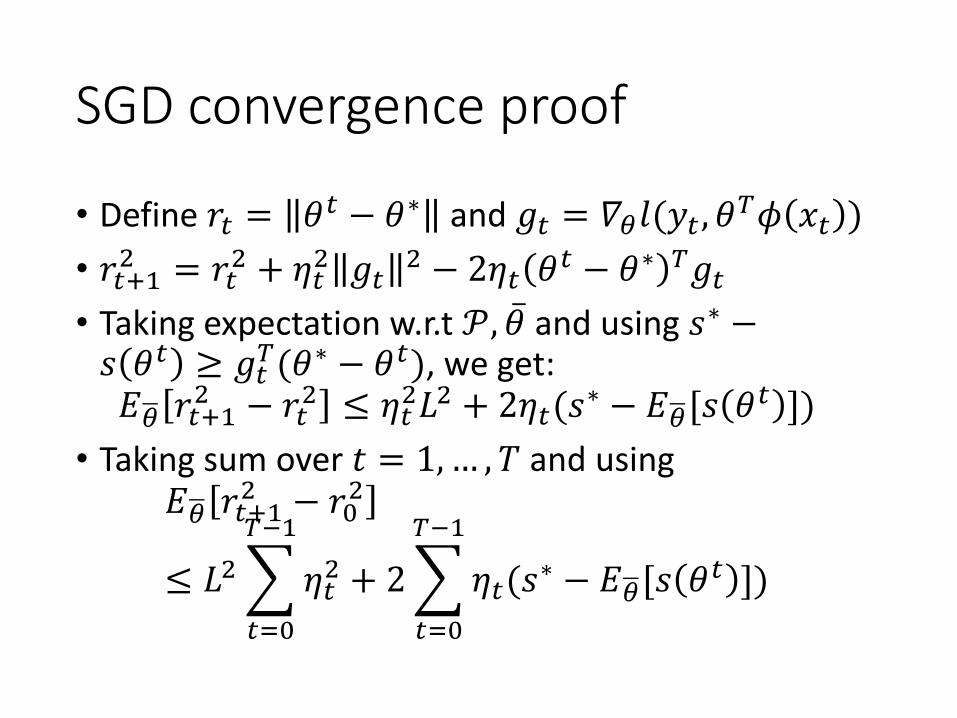
SGD convergence proof
• Define 𝑟𝑡 = 𝜃𝑡 − 𝜃∗ and 𝑔𝑡 = 𝛻𝜃𝑙(𝑦𝑡 , 𝜃
𝑇𝜙 𝑥𝑡 )
• 𝑟𝑡+12 = 𝑟𝑡
2 + 𝜂𝑡2 𝑔𝑡
2 − 2𝜂𝑡 𝜃𝑡 − 𝜃∗ 𝑇𝑔𝑡
• Taking expectation w.r.t 𝒫, 𝜃 and using 𝑠∗ −𝑠 𝜃𝑡 ≥ 𝑔𝑡
𝑇(𝜃∗ − 𝜃𝑡), we get:𝐸 𝜃 𝑟𝑡+1
2 − 𝑟𝑡2 ≤ 𝜂𝑡
2𝐿2 + 2𝜂𝑡(𝑠∗ − 𝐸 𝜃[𝑠 𝜃
𝑡 ])
• Taking sum over 𝑡 = 1,… , 𝑇 and using𝐸 𝜃 𝑟𝑡+1
2 − 𝑟02
≤ 𝐿2
𝑡=0
𝑇−1
𝜂𝑡2 + 2
𝑡=0
𝑇−1
𝜂𝑡(𝑠∗ − 𝐸 𝜃[𝑠 𝜃
𝑡 ])
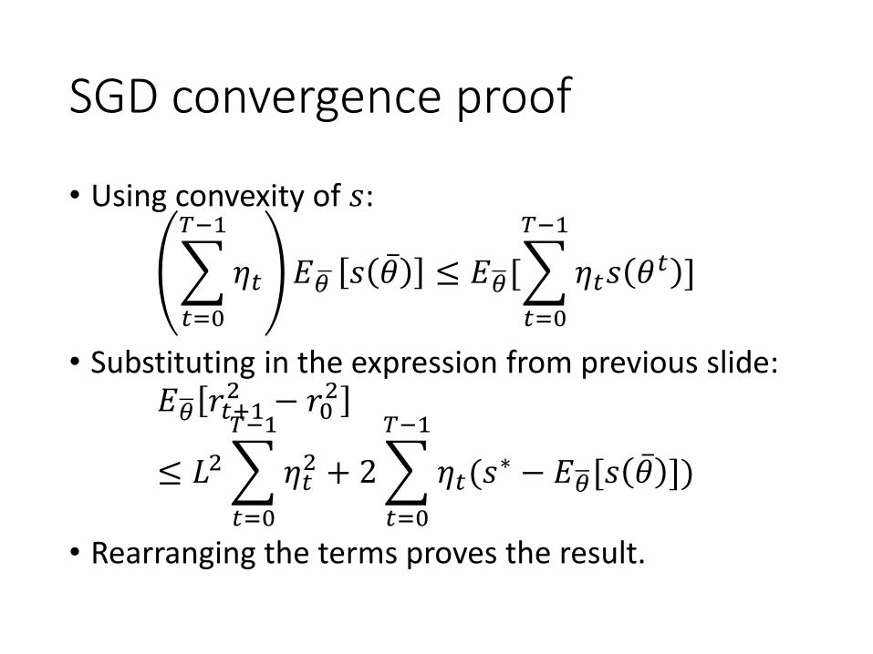
SGD convergence proof
• Using convexity of 𝑠:
𝑡=0
𝑇−1
𝜂𝑡 𝐸 𝜃 𝑠 𝜃 ≤ 𝐸 𝜃[
𝑡=0
𝑇−1
𝜂𝑡𝑠 𝜃𝑡 ]
• Substituting in the expression from previous slide:𝐸 𝜃 𝑟𝑡+1
2 − 𝑟02
≤ 𝐿2
𝑡=0
𝑇−1
𝜂𝑡2 + 2
𝑡=0
𝑇−1
𝜂𝑡(𝑠∗ − 𝐸 𝜃[𝑠 𝜃 ])
• Rearranging the terms proves the result.