Machine Learning

Fabrice Rossi

SAMMUniversité Paris 1 Panthéon Sorbonne

2018

Standard programming

Solving a task with a computerI input and output definitionI algorithm designI implementation

ExamplesI jpeg image converterI interactive 3D worldI computational fluid dynamicsI chess programI spam filtering (with e.g. SpamAssassin)

100% human design

2

Standard programming

Solving a task with a computerI input and output definitionI algorithm designI implementation

ExamplesI jpeg image converterI interactive 3D worldI computational fluid dynamicsI chess programI spam filtering (with e.g. SpamAssassin)

100% human design

2

Machine learning

Machine programmingI climbing one step in abstractionI designing programs with a programI output: a program that solves a taskI input?

Learning from examplesI input: a set of pairs (input, output)I output: a program gI if (x, y) is in the set, g should output y if given x as input (i.e.,

g(x) = y)I this is called supervised learningI example: produce SpamAssassin using tagged emails!

3

Machine learning

Machine programmingI climbing one step in abstractionI designing programs with a programI output: a program that solves a taskI input?

Learning from examplesI input: a set of pairs (input, output)I output: a program gI if (x, y) is in the set, g should output y if given x as input (i.e.,

g(x) = y)I this is called supervised learningI example: produce SpamAssassin using tagged emails!

3

Minimal formal model

Data spacesI X : input space (X ∈ X )I Y: output space (Y ∈ Y)

I if |Y| <∞: classificationI if Y = R: regression

ProgramsI mathematical version: a function g from X to YI running the program: g(X) = YI preferred term: model

Machine learning programI input: a data set D = {(Xi ,Yi)}1≤i≤N (or a data sequence)I output: a function from X to Y (a model)

4

Is machine learning feasible?

Yes!I strong theoretical guaranteesI Probably Approximately Correct (PAC) framework

I we look for g (the task solving program/model) in some class ofmodels

I is the class is not too complex, g can be recovered approximatelywith high probability given a reasonable amount (N) of input data

I Asymptotic frameworkI in addition the class of models can grow in complexity with the data

sizeI then the best possible g (no restriction) can be reached

asymptotically (almost surely in some cases): this is a consistencyproperty

How?

5

Is machine learning feasible?

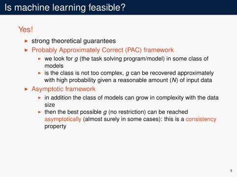
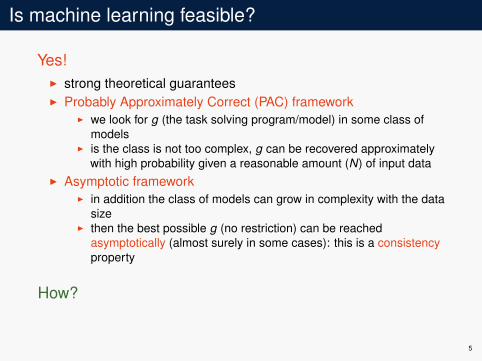
Yes!

I strong theoretical guaranteesI Probably Approximately Correct (PAC) framework

I we look for g (the task solving program/model) in some class ofmodels

I is the class is not too complex, g can be recovered approximatelywith high probability given a reasonable amount (N) of input data

I Asymptotic frameworkI in addition the class of models can grow in complexity with the data

sizeI then the best possible g (no restriction) can be reached

asymptotically (almost surely in some cases): this is a consistencyproperty

How?

5

Is machine learning feasible?

Yes!I strong theoretical guaranteesI Probably Approximately Correct (PAC) framework

I we look for g (the task solving program/model) in some class ofmodels

I is the class is not too complex, g can be recovered approximatelywith high probability given a reasonable amount (N) of input data

I Asymptotic frameworkI in addition the class of models can grow in complexity with the data

sizeI then the best possible g (no restriction) can be reached

asymptotically (almost surely in some cases): this is a consistencyproperty

How?

5

Is machine learning feasible?

Yes!I strong theoretical guaranteesI Probably Approximately Correct (PAC) framework

I we look for g (the task solving program/model) in some class ofmodels

I is the class is not too complex, g can be recovered approximatelywith high probability given a reasonable amount (N) of input data

I Asymptotic frameworkI in addition the class of models can grow in complexity with the data

sizeI then the best possible g (no restriction) can be reached

asymptotically (almost surely in some cases): this is a consistencyproperty

How?

5

Neighbors

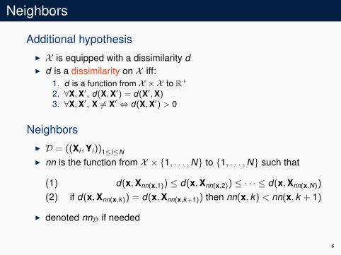
Additional hypothesisI X is equipped with a dissimilarity dI d is a dissimilarity on X iff:

1. d is a function from X × X to R+

2. ∀X,X′, d(X,X′) = d(X′,X)3. ∀X,X′, X 6= X′ ⇔ d(X,X′) > 0

NeighborsI D = ((Xi ,Yi))1≤i≤NI nn is the function from X × {1, . . . ,N} to {1, . . . ,N} such that

(1) d(x,Xnn(x,1)) ≤ d(x,Xnn(x,2)) ≤ · · · ≤ d(x,Xnn(x,N))

(2) if d(x,Xnn(x,k)) = d(x,Xnn(x,k+1)) then nn(x, k) < nn(x, k + 1)

I denoted nnD if needed

6

K nearest neighbors

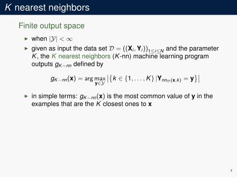
Finite output spaceI when |Y| <∞I given as input the data set D = ((Xi ,Yi))1≤i≤N and the parameter

K , the K nearest neighbors (K -nn) machine learning programoutputs gK−nn defined by

gK−nn(x) = argmaxy∈Y

∣∣{k ∈ {1, . . . ,K} |YnnD(x,k) = y}∣∣

I in simple terms: gK−nn(x) is the most common value of y in theexamples that are the K closest ones to x

ConsistencyI if X is a finite dimensional Banach space and |Y| = 2I then the K -nn method is consistent if K depends on N, KN , in

such a way that KN →∞ and KNN → 0

7

K nearest neighbors

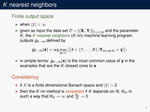
Finite output spaceI when |Y| <∞I given as input the data set D = ((Xi ,Yi))1≤i≤N and the parameter

K , the K nearest neighbors (K -nn) machine learning programoutputs gK−nn defined by

gK−nn(x) = argmaxy∈Y

∣∣{k ∈ {1, . . . ,K} |YnnD(x,k) = y}∣∣

I in simple terms: gK−nn(x) is the most common value of y in theexamples that are the K closest ones to x

ConsistencyI if X is a finite dimensional Banach space and |Y| = 2I then the K -nn method is consistent if K depends on N, KN , in

such a way that KN →∞ and KNN → 0

7

In practice?

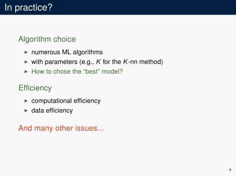
Algorithm choiceI numerous ML algorithmsI with parameters (e.g., K for the K -nn method)I How to chose the “best” model?

EfficiencyI computational efficiencyI data efficiency

And many other issues...

8

Machine learning vs AI

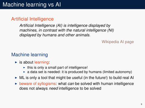
Artificial IntelligenceArtificial Intelligence (AI) is intelligence displayed bymachines, in contrast with the natural intelligence (NI)displayed by humans and other animals.

Wikipedia AI page

Machine learningI is about learning:

I this is only a small part of intelligence!I a data set is needed: it is produced by humans (limited autonomy)

I ML is only a tool that might be useful (in the future!) to build real AII beware of syllogisms: what can be solved with human intelligence

does not always need intelligence to be solved

9

Outline

Introduction

Loss and risk

10

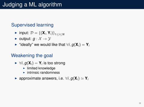
Judging a ML algorithm

Supervised learningI input: D = {(Xi ,Yi)}1≤i≤NI output: g : X → YI “ideally” we would like that ∀i ,g(Xi) = Yi

Weakening the goalI ∀i ,g(Xi) = Yi is too strong

I limited knowledgeI intrinsic randomness

I approximate answers, i.e. ∀i ,g(Xi) ' Yi

11

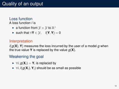
Quality of an output

Loss functionA loss function l is

I a function from Y × Y to R+

I such that ∀Y ∈ Y, l(Y,Y) = 0

Interpretationl(g(X),Y) measures the loss incurred by the user of a model g whenthe true value Y is replaced by the value g(X).

Weakening the goalI ∀i ,g(Xi) = Yi is replaced byI ∀i , l(g(Xi),Yi) should be as small as possible

12

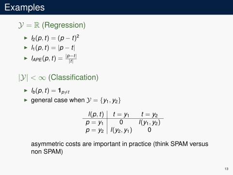
Examples

Y = R (Regression)I l2(p, t) = (p − t)2

I l1(p, t) = |p − t |I lAPE(p, t) =

|p−t||t|

|Y| <∞ (Classification)I lb(p, t) = 1p 6=t

I general case when Y = {y1, y2}

l(p, t) t = y1 t = y2

p = y1 0 l(y1, y2)p = y2 l(y2, y1) 0

asymmetric costs are important in practice (think SPAM versusnon SPAM)

13

Quality of a model

From local to globalI loss functions work at a local scale: what happens for one inputI we need a global assessment of a model g: how will the model

behave if deployed?

I expected loss

Empirical riskI simple aggregation of local losses: average lossI the empirical risk of a model g on a data set D = {(Xi ,Yi)}1≤i≤N

for a loss function l is

Rl(g,D) =1N

N∑i=1

l(g(Xi),Yi) =1|D|

∑(x,y)∈D

l(g(x),y)

I a good model has a low empirical risk

14

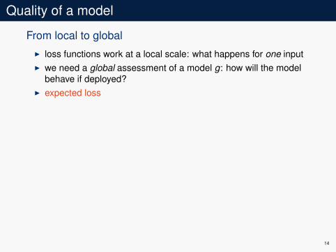
Quality of a model

From local to globalI loss functions work at a local scale: what happens for one inputI we need a global assessment of a model g: how will the model

behave if deployed?I expected loss

Empirical riskI simple aggregation of local losses: average lossI the empirical risk of a model g on a data set D = {(Xi ,Yi)}1≤i≤N

for a loss function l is

Rl(g,D) =1N

N∑i=1

l(g(Xi),Yi) =1|D|

∑(x,y)∈D

l(g(x),y)

I a good model has a low empirical risk

14

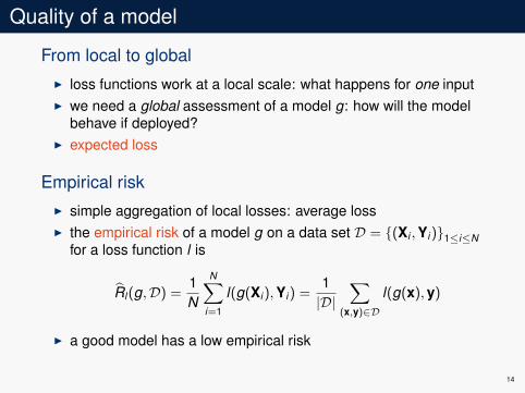
Quality of a model

From local to globalI loss functions work at a local scale: what happens for one inputI we need a global assessment of a model g: how will the model

behave if deployed?I expected loss

Empirical riskI simple aggregation of local losses: average lossI the empirical risk of a model g on a data set D = {(Xi ,Yi)}1≤i≤N

for a loss function l is

Rl(g,D) =1N

N∑i=1

l(g(Xi),Yi) =1|D|

∑(x,y)∈D

l(g(x),y)

I a good model has a low empirical risk

14

Data science intermezzo

Loss functionsI should not be chosen lightlyI have complex consequences, for instance

I asymmetric losses can be seen as example weightingI APE loss induces underestimation

I a good data scientist knows how to translate objectives into lossfunctions

Empirical riskI is only an average: does not rule out extreme behaviorI in particular, the actual loss can strongly vary with the “location” of

x in XI reporting only the empirical risk is not sufficient!

15

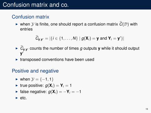
Confusion matrix and co.

Confusion matrixI when Y is finite, one should report a confusion matrix C(D) with

entries

Cy,y′ = |{i ∈ {1, . . . ,N} | g(Xi) = y and Yi = y′}|

I Cy,y′ counts the number of times g outputs y while it should outputy′

I transposed conventions have been used

Positive and negativeI when Y = {−1,1}I true positive: g(Xi) = Yi = 1I false negative: g(Xi) = −Yi = −1I etc.

16

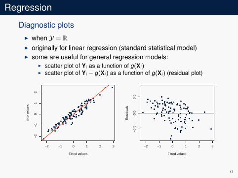
Regression

Diagnostic plotsI when Y = RI originally for linear regression (standard statistical model)I some are useful for general regression models:

I scatter plot of Yi as a function of g(Xi)I scatter plot of Yi − g(Xi) as a function of g(Xi) (residual plot)

−2 −1 0 1 2 3

−2

−1

01

2

Fitted values

True

val

ues

−2 −1 0 1 2 3

−0.

50.

00.

5

Fitted values

Res

idua

ls

17

Generalization

New dataI assume g is such as Rl(g,D) is smallI what can we expect on a new data set Rl(g,D′)?I generalization performancesI if g is learned on D and Rl(g,D)� Rl(g,D′), g is overfitting

Mathematical modelI stationary behavior: D ' D′I hypotheses:

I observations are random variables with values in X × YI they are distributed according to a fixed and unknown distribution DI observations are independent

18

Generalization

New dataI assume g is such as Rl(g,D) is smallI what can we expect on a new data set Rl(g,D′)?I generalization performancesI if g is learned on D and Rl(g,D)� Rl(g,D′), g is overfitting

Mathematical modelI stationary behavior: D ' D′I hypotheses:

I observations are random variables with values in X × YI they are distributed according to a fixed and unknown distribution DI observations are independent

18

Risk

Data set revisitedI D = ((Xi ,Yi))1≤i≤NI (Xi ,Yi) ∼ DI D ∼ DN (product distribution)

Risk of a modelI The risk of g for the loss function l is

Rl(g) = E(X,Y)∼D(l(g(X),Y))

I we should write Rl(g,D)

I the empirical risk Rl(g,D) is a random variable

I if g is fixed or independent from D, then Rl(g,D)a.s.−−−−−→|D|→∞

Rl(g)

(strong law of large numbers)

19

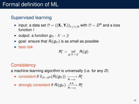
Formal definition of ML

Supervised learningI input: a data set D = ((Xi ,Yi))1≤i≤N with D ∼ DN and a loss

function lI output: a function gD : X → YI goal: ensure that Rl(gD) is as small as possibleI best risk

R∗l = infg:X→Y

Rl(g)

Consistencya machine learning algorithm is universally (i.e. for any D)

I consistent if ED∼DN (Rl(gD)) −−−−→N→∞

R∗l

I strongly consistent if Rl(gD)a.s.−−−−→

N→∞R∗l

20

ML and statistical models

Statistical modelsI specification for D (in general parametric)I estimation with maximum likelihoodI numerous variants (especially Bayesian approaches)

Very different philosophiesI Machine Learning

I performance orientedI universal consistencyI limited post learning tuning, exploration, interpretation, etc.

I Statistical modelsI strong hypothesesI bad behavior under wrong specificationI very rich framework for post estimation exploitation

I but many links!

21

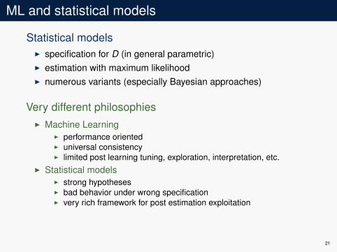
ML and statistical models

Statistical modelsI specification for D (in general parametric)I estimation with maximum likelihoodI numerous variants (especially Bayesian approaches)

Very different philosophiesI Machine Learning

I performance orientedI universal consistencyI limited post learning tuning, exploration, interpretation, etc.

I Statistical modelsI strong hypothesesI bad behavior under wrong specificationI very rich framework for post estimation exploitation

I but many links!

21

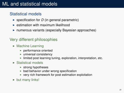
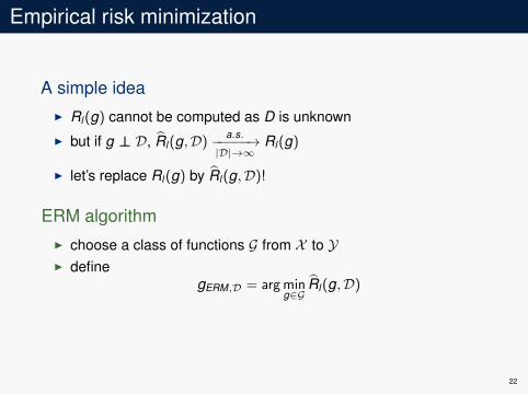
Empirical risk minimization

A simple ideaI Rl(g) cannot be computed as D is unknown

I but if g ⊥⊥ D, Rl(g,D)a.s.−−−−−→|D|→∞

Rl(g)

I let’s replace Rl(g) by Rl(g,D)!

ERM algorithmI choose a class of functions G from X to YI define

gERM,D = argming∈G

Rl(g,D)

22

Empirical risk and learning

Empirical risk can be misleadingI for the 1-nn, in general:

Rl(g1−nn,D) = 0

if g1−nn has been constructed on DI indeed if all the Xi are distinct, nn(Xi ,1) = i and thus

g1−nn(Xi) = Yi

I unrealistic value for Rl(g1−nn)

Source of the problemI the strong law of large numbers applies when the random

variables are independentI the (l(gD(Xi),Yi))1≤i≤N are dependent variables!

23

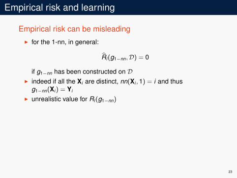
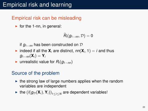
Empirical risk and learning

Empirical risk can be misleadingI for the 1-nn, in general:

Rl(g1−nn,D) = 0

if g1−nn has been constructed on DI indeed if all the Xi are distinct, nn(Xi ,1) = i and thus

g1−nn(Xi) = Yi

I unrealistic value for Rl(g1−nn)

Source of the problemI the strong law of large numbers applies when the random

variables are independentI the (l(gD(Xi),Yi))1≤i≤N are dependent variables!

23

Methodology

Does ERM work?I Yes!

I but one needs to control the complexity of the class of models GI this is a form of regularization: one cannot look for the model in an

arbitrary class of modelsI this will be addressed latter in the course

Basic element for a solutionI apply the ML method to a data set D, the learning setI evaluate its risk on another independent data set D′

I in summary: Rl(gD,D′)

24

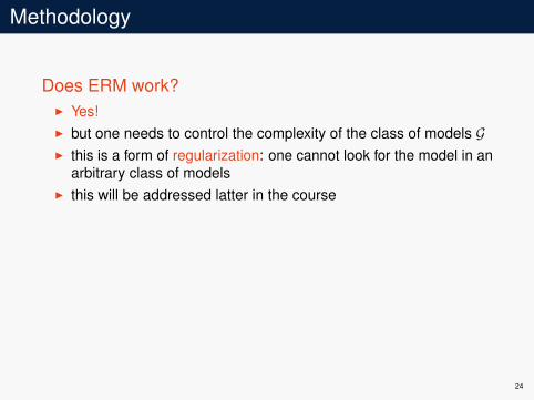
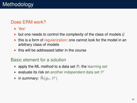
Methodology

Does ERM work?I Yes!I but one needs to control the complexity of the class of models GI this is a form of regularization: one cannot look for the model in an

arbitrary class of modelsI this will be addressed latter in the course

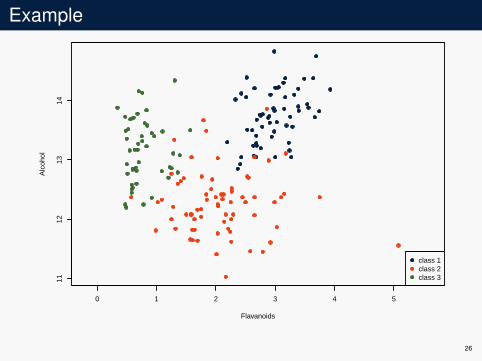
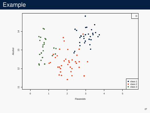
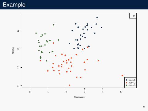
Basic element for a solutionI apply the ML method to a data set D, the learning setI evaluate its risk on another independent data set D′

I in summary: Rl(gD,D′)

24

Methodology

Does ERM work?I Yes!I but one needs to control the complexity of the class of models GI this is a form of regularization: one cannot look for the model in an

arbitrary class of modelsI this will be addressed latter in the course

Basic element for a solutionI apply the ML method to a data set D, the learning setI evaluate its risk on another independent data set D′

I in summary: Rl(gD,D′)

24

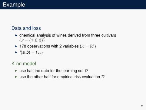
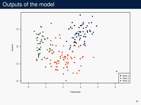
Example

Data and lossI chemical analysis of wines derived from three cultivars

(Y = {1,2,3})I 178 observations with 2 variables (X = R2)I l(a,b) = 1a 6=b

K-nn modelI use half the data for the learning set DI use the other half for empirical risk evaluation D′

25

Example

0 1 2 3 4 5

1112

1314

Flavanoids

Alc

ohol

class 1class 2class 3

26

Example

0 1 2 3 4 5

1112

1314

Flavanoids

Alc

ohol

class 1class 2class 3

D

27

Example

0 1 2 3 4 5

1112

1314

Flavanoids

Alc

ohol

class 1class 2class 3

D′

28

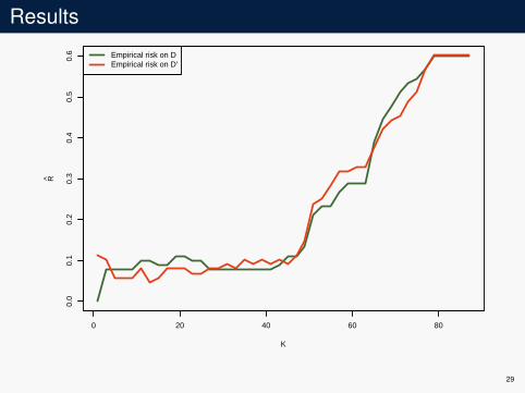
Results

0 20 40 60 80

0.0

0.1

0.2

0.3

0.4

0.5

0.6

K

REmpirical risk on DEmpirical risk on D′

29

Outputs of the model

0 1 2 3 4 5

1112

1314

Flavanoids

Alc

ohol

class 1class 2class 3

30

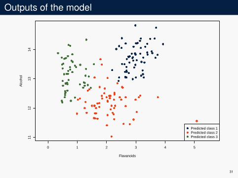
Outputs of the model

0 1 2 3 4 5

1112

1314

Flavanoids

Alc

ohol

Predicted class 1Predicted class 2Predicted class 3

31

Basic general framework

1. split the data into D (learning), D′ (validation) and D′′ (test)2. for each machine learning algorithm A under study

2.1 for each value θ of the parameters of the algorithm2.1.1 compute the model using θ on D, gA,θ,D2.1.2 compute Rl (gA,θ,D,D′)

3. chose the best algorithm with the best parameter, A∗ and θ∗

(according to Rl(.,D′))4. compute the best model g∗ = gA∗,θ∗,D∪D′

5. compute Rl(g∗,D′′)

Goals of this courseI describe state-of-the-art alternative for the algorithmsI study some theoretical aspects, e.g. empirical risk minimizationI describe better frameworks

32

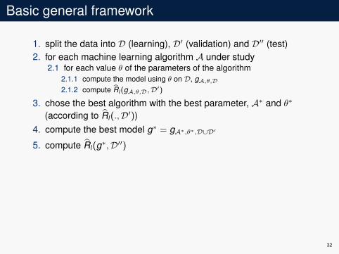
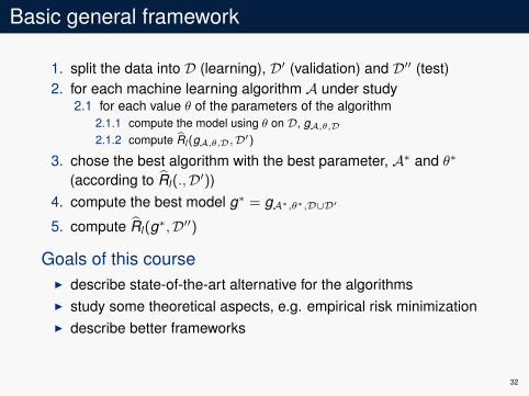
Basic general framework

1. split the data into D (learning), D′ (validation) and D′′ (test)2. for each machine learning algorithm A under study

2.1 for each value θ of the parameters of the algorithm2.1.1 compute the model using θ on D, gA,θ,D2.1.2 compute Rl (gA,θ,D,D′)

3. chose the best algorithm with the best parameter, A∗ and θ∗

(according to Rl(.,D′))4. compute the best model g∗ = gA∗,θ∗,D∪D′

5. compute Rl(g∗,D′′)

Goals of this courseI describe state-of-the-art alternative for the algorithmsI study some theoretical aspects, e.g. empirical risk minimizationI describe better frameworks

32

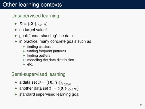
Other learning contexts

Unsupervised learningI D = ((Xi)1≤i≤N)

I no target value!I goal: “understanding” the dataI in practice, many concrete goals such as

I finding clustersI finding frequent patternsI finding outliersI modeling the data distributionI etc.

Semi-supervised learningI a data set D = ((Xi ,Yi))1≤i≤NI another data set D = ((X′i )1≤i≤N′)

I standard supervised learning goal

33

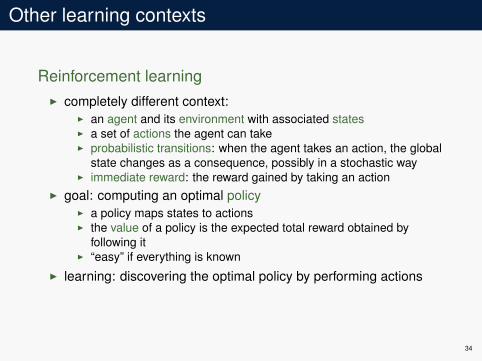
Other learning contexts

Reinforcement learningI completely different context:

I an agent and its environment with associated statesI a set of actions the agent can takeI probabilistic transitions: when the agent takes an action, the global

state changes as a consequence, possibly in a stochastic wayI immediate reward: the reward gained by taking an action

I goal: computing an optimal policyI a policy maps states to actionsI the value of a policy is the expected total reward obtained by

following itI “easy” if everything is known

I learning: discovering the optimal policy by performing actions

34

Licence

This work is licensed under a Creative CommonsAttribution-ShareAlike 4.0 International License.

http://creativecommons.org/licenses/by-sa/4.0/

35

Version

Last modification: 2018-02-05By: Fabrice Rossi (Fabrice.Rossi@apiacoa.org)Git hash: 1b0849e751c9b992d0eb957563be19636769feaa

36