Embed Size (px)
Citation preview
Time Step Simulationp
[email protected] South First Street2001 South First Street pp @phttp://www.powerworld.comChampaign, Illinois 61820
+1 (217) 384.6330Champaign, Illinois 61820+1 (217) 384.6330

Time Step Simulation
• It is often useful to assess how power system
Time Step Simulation
p yquantities vary hour by hour due to changes in load, generation, transmission line status, etc.
• The Time Step Simulation (TSS) allows you to obtain power flow, OPF, and SCOPF solutions for a list of time
i t f hi h i t ( i ) d t h bpoints for which input (scenario) data has been specified.
• It also allows you to model actions that occur at• It also allows you to model actions that occur at specific times, as well as periodic actions.
2© 2012 PowerWorld CorporationM7: Time Step Simulation

Time Step Simulation
• In this section we’ll learn how to:
Time Step Simulation
In this section we ll learn how to:– Set up and maintain a list of time points
– Specify time point input data
– Specify scheduled input data
– Customize the results we want to store from the l isolution
– Run “continuous” and “timed” simulations
• Open the B7flat PWB case To access the Time Step• Open the B7flat.PWB case. To access the Time Step Simulation Dialog, in Run Mode, go to the Toolsribbon tab and select Time Step Simulation
3© 2012 PowerWorld CorporationM7: Time Step Simulation
ribbon tab and select Time Step Simulation.

Inserting New Time Points
• The first step in setting up a Time Step
Inserting New Time Points
The first step in setting up a Time Step Simulation is to define a list of time points. – This is a list of points in time for which– This is a list of points in time for which Simulator will obtain solutions.
• In the Time Step Simulation dialog right• In the Time Step Simulation dialog, right‐click on the grid and select Insert New Timepoint(s) or press the Insert TimeTimepoint(s), or press the Insert Time Points button.
4© 2012 PowerWorld CorporationM7: Time Step Simulation

Inserting New Time PointsInserting New Time Points
As an example, assume we want to simulate 24 hours,
Click to select the
As an example, assume we want to simulate 24 hours, starting on May 18, 2006 at 1:00 AM
date from a calendar component
Number of timeNumber of time points that will be inserted
Specify the interval between time points.Maximum resolution is 1
5© 2012 PowerWorld CorporationM7: Time Step Simulation
second.

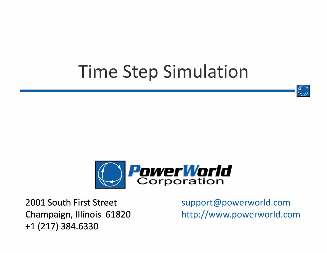
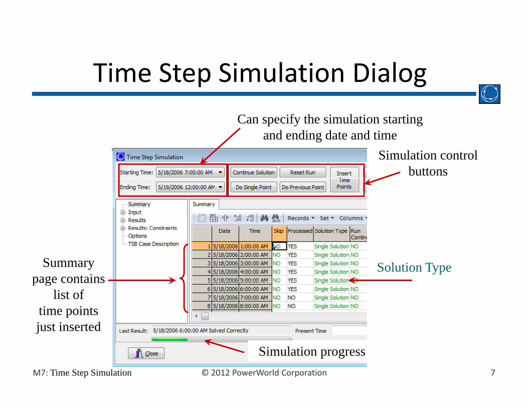
Inserting New Time Points• After Inserting the Time Points, the Time Step
Inserting New Time Points
Simulation dialog looks like this:
By default dialog shows
the SSummary
page
6© 2012 PowerWorld CorporationM7: Time Step Simulation
Time Step Simulation DialogTime Step Simulation DialogCan specify the simulation starting
Simulation control buttons
and ending date and time
Summary page contains
Solution Typepage contains
list of time pointsjust inserted
7© 2012 PowerWorld CorporationM7: Time Step Simulation
j
Simulation progress

Summary Page:Controlling SolutionControlling Solution
During the simulation you can skip a Time PointTi P ior you can pause at a Time Point
• The Time Point Solution Type can be:– Single Solution: Same as hitting the single solution button, but
would act on the corresponding time point.would act on the corresponding time point.
– Unconstrained OPF
– Optimal Power Flow (OPF)
S it C t i d O ti l P Fl (SCOPF)
8© 2012 PowerWorld CorporationM7: Time Step Simulation
– Security Constrained Optimal Power Flow (SCOPF)
• Different time points can have different solution types

Time Step Simulation Dialog.TSB file
Time Step Simulation Dialog
The input data and Deletes res lts inp t andControl The input data and the results of the Time Step Si l ti b
Deletes results, input and scheduled input data, and
the list of time points
Simulation can be saved in a Time Series Binary (*.TSB) file.(Time Step Actions saved in PWB)saved in .PWB)
9© 2012 PowerWorld CorporationM7: Time Step Simulation

Summary Page: Script CommandsScript Commands
• You can specify pre‐ and post script commands for each time point.
• This allows you to perform almost every possible Simulator• This allows you to perform almost every possible Simulator action before and after a time point is solved.
• Typical actions are running contingency analysis or saving ti l t f lt
10© 2012 PowerWorld CorporationM7: Time Step Simulation
particular set of results.

Summary Page:Script Command Tips
• It is a good idea to first test the script commands in script
Script Command Tips
g p pmode, to avoid potential syntax errors.
• To edit the script command cell, double‐click on the cell.You can copy/paste from the cells as usual– You can copy/paste from the cells as usual
– You can also copy/paste from excel or the clipboard.
• To delete a script command, double‐click and hit the Delete B k b ttor Backspace buttons.
• To clear all the scripts commands in a column, right‐click on the grid and select Set/Toggle/Columns Set All Values To. Then just press OK without typing anything in the dialog.
11© 2012 PowerWorld CorporationM7: Time Step Simulation
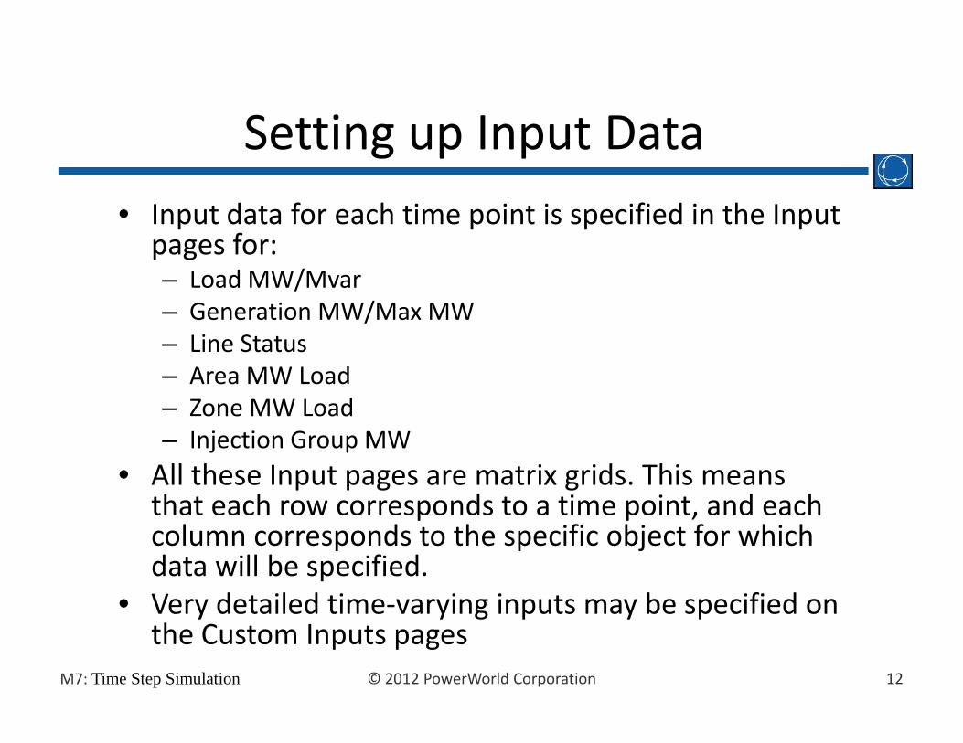
Setting up Input Data• Input data for each time point is specified in the Input
Setting up Input Data
pages for:– Load MW/Mvar– Generation MW/Max MW– Line Status– Area MW Load– Zone MW Load– Injection Group MW
• All these Input pages are matrix grids. This means that each row corresponds to a time point, and eachthat each row corresponds to a time point, and each column corresponds to the specific object for which data will be specified.
• Very detailed time‐varying inputs may be specified on
12© 2012 PowerWorld CorporationM7: Time Step Simulation
• Very detailed time‐varying inputs may be specified on the Custom Inputs pages

Setting up Input Data
• Thus we need to explicitly tell Simulator which
Setting up Input Data
Thus we need to explicitly tell Simulator which generators, loads, etc. will have input data.– The objects that do not have input data (or scheduled i t d t ) ill k th l f thinput data) will keep the values from the case.
• The matrix grids will have one column for the input data of each object.input data of each object.
• In the B7flat.pwb case, suppose that we want to specify Load MW data for Loads 2 and 3. – In the Input page MW Loads page, right‐click and select Time Point records Insert/Scale Load Column(s)
13© 2012 PowerWorld CorporationM7: Time Step Simulation
Column(s)
Setting up Input DataSetting up Input Data
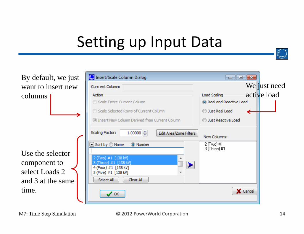
By default, we just want to insert new columns
We just need active load
Use the selector t tcomponent to
select Loads 2 and 3 at the same time
14© 2012 PowerWorld CorporationM7: Time Step Simulation
time.

Setting up Input DataSetting up Input Data
The columnsThe columns will contain zeros by default. Thosedefault. Those will need to be filled with correct data.
In order to specify time point values, we can:1. Enter the values manually (as shown in the Figure) 2. Paste values from Excel (Copy the headers to Excel first).3. Derive the values from another column.4 Scale the column values
15© 2012 PowerWorld CorporationM7: Time Step Simulation
4. Scale the column values.
Setting up Input Data
Example:
Setting up Input Data
Example: • We have specified some values for Loads 2 and 3 (as shown in the previous slide).
l d f d f d• Suppose we also need to specify input data for Loads 4 and 5, and know that those vary as Load 3, but are 90% of it. – We can derive the values for Loads 4 and 5 from Load 3.
• Right‐click on column for Load 3 and select Time Point records Insert/Scale Load Column(s)Point records Insert/Scale Load Column(s).– Column 3 will now be the Current Column
16© 2012 PowerWorld CorporationM7: Time Step Simulation

Setting up Input DataSetting up Input Data
C l 3 bColumn 3 becomes the current column
Loads 4 and 5 will be 90% of Load 3
Use the selector t t l tcomponent to select
Loads 4 and 5, whose values will be derived from Load 3
17© 2012 PowerWorld CorporationM7: Time Step Simulation
from Load 3.

Setting up Input Data
• The Input Load MW page now looks like this:
Setting up Input Data
• The Input Load MW page now looks like this:
18© 2012 PowerWorld CorporationM7: Time Step Simulation
Columns derived as 90% of Load 3

Setting up Input Data
• We can use the column plot to check our input data.
Setting up Input Data
p p• The plot column function of Case Information Displays
becomes a plot versus date time when used from Time Step Simulation matrix grids. p g
To plot a column, right-click on the column and select Set/Toggle/Columns
Plot Column from the Local Menu.You can also drag theYou can also drag the mouse across several columns to plot multiple columns. The Load MW
19© 2012 PowerWorld CorporationM7: Time Step Simulation
for Loads 2-5 looks like this.

Setting up Input Data
• Since we have spent some time defining our input
Setting up Input Data
• Since we have spent some time defining our input data, it is probably good to save the input data in the .TSB file.
• Press the Save TSB File button, and save the data as B7TSS.TSB
20© 2012 PowerWorld CorporationM7: Time Step Simulation

Setting up Input Data
• In the same manner as we did for load MW,
Setting up Input Data
In the same manner as we did for load MW, hourly data for other quantities would be specified in the corresponding pages:
Mvar Loads– Mvar Loads– Gen Actual MW– Gen Max MW– Line Status– Area Loads– Zone Loads– Injection Groups
• Recall that you can use the selector to create multiple columns at a time and you can copy/
21© 2012 PowerWorld CorporationM7: Time Step Simulation
multiple columns at a time, and you can copy/ paste the input data from Excel.

Setting Up Results• During the time step simulation, Simulator
Setting Up Resultsg p
obtains a PF/OPF/SCOPF solution for each time point.
• The amount of information that is generated mayThe amount of information that is generated may be significant since each time point can potentially contain the information of a solved PF, OPF or SCOPF caseOPF, or SCOPF case.– For large systems, storing all these information may be limited by memory.
T i ll d ’ d i ll h• Typically, you don’t need to examine all the system quantities. The Time Step Simulation requires you to explicitly define which quantities
22© 2012 PowerWorld CorporationM7: Time Step Simulation
you want to explore.

Setting Up Results
• Select the Results page:
Setting Up Results
p gModify the Results Definitions
Results Display Options
Result pagesBy default no
bj t h
23© 2012 PowerWorld CorporationM7: Time Step Simulation
objects are shown

Setting Up Results
• Press the View/Modify Result Definitions button
Setting Up Results
Press the View/Modify Result Definitions button to tell Simulator the quantities you want to store.
• You will need to specify:p y– The type of object for which results must be saved (buses, generators, etc.)
– The individual objects whose fields will be saved (Bus 1, Bus 2, etc.)
– The fields that will be saved for each type of objects– The fields that will be saved for each type of objects (Bus pu volt, etc.)
24© 2012 PowerWorld CorporationM7: Time Step Simulation
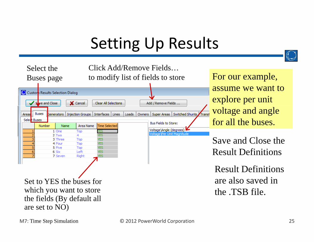
Setting Up ResultsSetting Up ResultsClick Add/Remove Fields… t dif li t f fi ld t t For our example
Select the B to modify list of fields to store For our example,
assume we want to explore per unit
Buses page
voltage and angle for all the buses.
Save and Close the Result Definitions
R lt D fi itiSet to YES the buses for which you want to store th fi ld (B d f lt ll
Result Definitions are also saved in the .TSB file.
25© 2012 PowerWorld CorporationM7: Time Step Simulation
the fields (By default all are set to NO)

Running the Simulation
• Now that we have set input data and specified which
Running the Simulation
p presults we need to store, we can run the simulation.
• Simulator will obtain a solution for each time point d di th l ti tdepending on the solution type.
• In order to start the simulation, press the Do Run button.
• During the simulation, you will see how the Last Result box g , yand the Progress Bar are updated.
26© 2012 PowerWorld CorporationM7: Time Step Simulation

Running the Simulation
• Simulator will do the following at each time point:
Running the Simulation
g p– Look at the time point skip/pause flag and act accordinglyR i t d if it ifi d– Run a pre‐script command if it was specified
– Apply time point and scheduled input data.• We’ll learn how to set scheduled input data later on.
– Obtain the PF/OPF/SCOPF solution– Set the Processed flag in the Summary pageUpdate the Last Result and Progress Bar indicating the– Update the Last Result and Progress Bar indicating the status of the solution.
– Write the results to the Result pages
27© 2012 PowerWorld CorporationM7: Time Step Simulation
– Run a post‐script command if it was specified

Exploring Results
• For our example the Buses page of the Results shows
Exploring Results
• For our example, the Buses page of the Results shows bus voltages and angles.
• The results can be grouped by objects or by fields.
BUS 1 BUS 2
28© 2012 PowerWorld CorporationM7: Time Step Simulation
Exploring Results
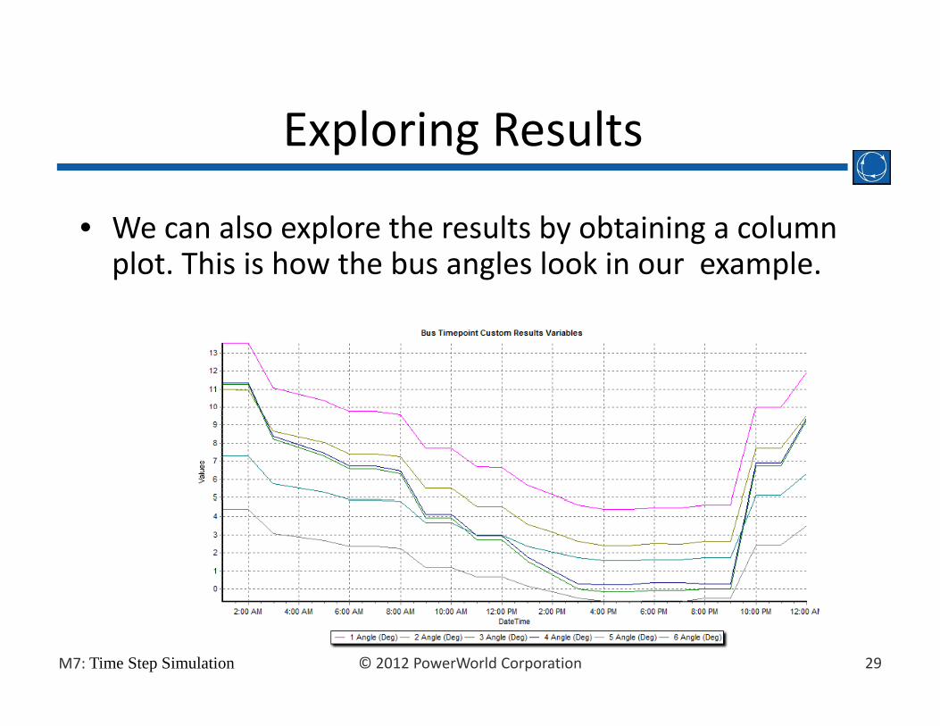
• We can also explore the results by obtaining a column
Exploring Results
• We can also explore the results by obtaining a column plot. This is how the bus angles look in our example.
29© 2012 PowerWorld CorporationM7: Time Step Simulation

Specifying Scheduled Input Data
• Besides time point input data, the Time Step
Specifying Scheduled Input Data
p p , pSimulation allows you to specify scheduled data.
• Scheduled data is used for data that more ll l l h hnaturally spans multiple time points rather than
being defined at each time point– Line statusesLine statuses– Generator, load, capacitor and reactor statuses– MW levels of scheduled transactions– Number of capacitor/reactor blocks– Generator voltage set pointsetc
30© 2012 PowerWorld CorporationM7: Time Step Simulation
– etc.
Specifying Scheduled Input Data• Schedule input data requires a schedule and a
Specifying Scheduled Input Datap q
schedule subscription.• The schedule defines how a quantity varies in time (just a shape) It is a list of time pointstime (just a shape). It is a list of time points together with Numeric or Yes/No values.
• By subscribing an object field (Line status, Gen MW T ti MW l l t ) t h d lMW, Transaction MW level, etc.) to a schedule, we can make this object field vary according to the shape of the schedule.
• Schedules are implemented as sets of actions that are applied to the power flow case at the next available time point.
31© 2012 PowerWorld CorporationM7: Time Step Simulation
available time point.

Specifying Scheduled Input DataSpecifying Scheduled Input Data
ScheduleValue
Time Point List
t
Object FieldSubscription
t
jGen MW
32© 2012 PowerWorld CorporationM7: Time Step Simulationt
Defining a Schedule
• Schedules:
Defining a Schedule
Schedules:– Are Numeric, Yes/No, or Text
Can be made periodic by specifying them to– Can be made periodic by specifying them to repeat the shape with a certain period.
– Can have start and end validity dates (used– Can have start and end validity dates (used normally for periodic schedules).
• To define a schedule go to the Input page• To define a schedule go to the Input page Schedules page, right‐click on the grid,
and select Insert New Schedule
33© 2012 PowerWorld CorporationM7: Time Step Simulation
and select Insert New Schedule.

Defining a ScheduleDefining a ScheduleSchedule name must be unique Identifies main
characteristics of schedule
Settings for periodic
Shortcut buttons allow easy
characteristics of schedule
periodic Schedules
easy definition of the schedule date times
i d
Date times don’t need to coincide
date times
Date time and numeric values define the shape of
with the date times of the list of time points
34© 2012 PowerWorld CorporationM7: Time Step Simulation
the shape of the schedule
(Summary page)

Defining a Schedule Subscription
• Most enterable fields from the following object
Defining a Schedule Subscription
Most enterable fields from the following object types can subscribe to schedules: Generators, Loads, Line/transformers, Shunts, Areas,
i dTransactions, and Zones• Numeric fields subscribe to Numeric Schedules, Boolean fields subscribe to Yes/No schedules andBoolean fields subscribe to Yes/No schedules, and Custom Strings and Memo fields subscribe to Text schedules.
• To define a schedule subscription, go to the Input page Sched Subscriptions page, right‐click on the grid and select Insert New Subscription
35© 2012 PowerWorld CorporationM7: Time Step Simulation
the grid, and select Insert New Subscription.
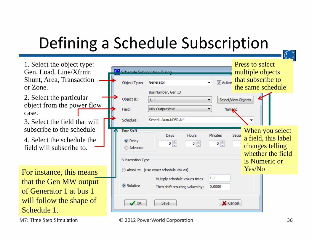
Defining a Schedule SubscriptionDefining a Schedule Subscription 1. Select the object type: Gen, Load, Line/Xfrmr,
Press to select multiple objects , , ,
Shunt, Area, Transactionor Zone.2. Select the particular object from the power flow
p jthat subscribe to the same schedule
object from the power flow case.3. Select the field that will subscribe to the schedule When you select
fi ld hi l b l4. Select the schedule the field will subscribe to.
a field, this label changes telling whether the field is Numeric or Yes/NoFor instance, this means
that the Gen MW output of Generator 1 at bus 1
36© 2012 PowerWorld CorporationM7: Time Step Simulation
will follow the shape of Schedule 1.

Defining a Schedule SubscriptionDefining a Schedule Subscription
Schedule actions are applied with the specified delay
Subscriptions to numeric schedules can modify the schedule values:Actual Value = Multiplier *S h d V l + V l Shift
37© 2012 PowerWorld CorporationM7: Time Step Simulation
*Sched Value + Value Shift

Example: Scheduled Input Data
• In the B7Flat.pwb case, the following input data p , g pis known for Gen 1 and line 2 to 3. The generator values occur every day.
Hour Gen 1MW Hour Line 2-3 Status1:00 AM 60 MW 4:00 AM Open7:00 AM 80 MW 2:00 PM Closed1:00 PM 120 MW7 00 PM 100 MW
• We want to create the schedules and schedules subscriptions needed to model these varying
7:00 PM 100 MW
38© 2012 PowerWorld CorporationM7: Time Step Simulation
subscriptions needed to model these varying quantities.

Example: Schedules
• For the generator, g ,we create a periodic schedule with period = 1 dayperiod = 1 day.
• The schedule is numeric.
• The schedule has 4 time points.
39© 2012 PowerWorld CorporationM7: Time Step Simulation

Example: Schedule Subscriptions
• Then we subscribe the Gen MW output filed of generator 1, g ,ID 1 to Sched1.
Th i d l• There is no delay• The field takes the
exact values of the numeric schedule.
Note: Gen1 needs to be Off-AGC in order to keep the scheduled MW
40© 2012 PowerWorld CorporationM7: Time Step Simulation
output. Manually set or use option

Example: Schedules
h• For the transmission line, we create a non‐periodic pschedule
• The schedule type is Yes/No.
• The schedule has 2The schedule has 2 time points. Line will open at 4 AM and ill l t 2 PM
41© 2012 PowerWorld CorporationM7: Time Step Simulation
will close at 2 PM.

Example: Schedule Subscriptions
• Then we subscribe the Status of Transmission Line 2Transmission Line 2 to 3, circuit 1 to Sched2.
• There is no delay
• Let us go ahead and rerun the Time Step
42© 2012 PowerWorld CorporationM7: Time Step Simulation
Time Step Simulation.
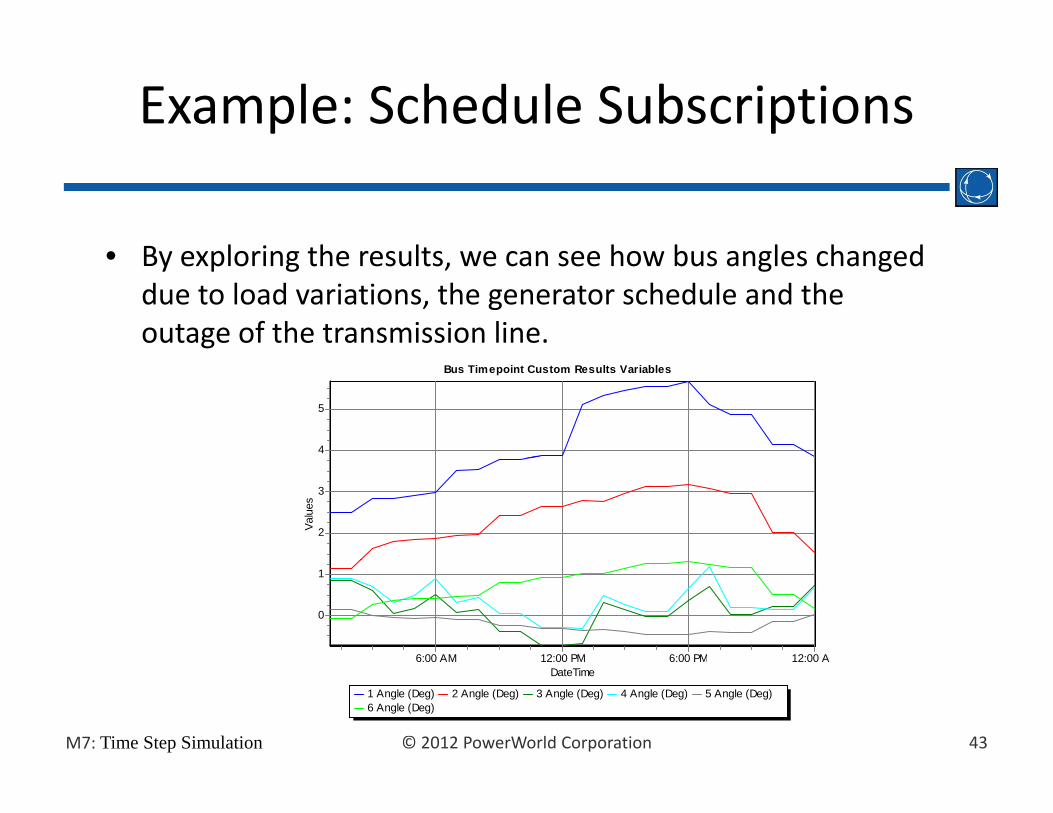
Example: Schedule Subscriptions
• By exploring the results we can see how bus angles changed• By exploring the results, we can see how bus angles changed due to load variations, the generator schedule and the outage of the transmission line.
Bus Timepoint Custom Results Variables
5
4
Valu
es
3
2
12:00 A6:00 PM12:00 PM6:00 AM
1
0
43© 2012 PowerWorld CorporationM7: Time Step Simulation
1 Angle (Deg) 2 Angle (Deg) 3 Angle (Deg) 4 Angle (Deg) 5 Angle (Deg)6 Angle (Deg)
DateTime

Schedule Subscriptions
• The advantage of schedules and schedule
Schedule Subscriptions
• The advantage of schedules and schedule subscriptions is that power systems tend to have many quantities that follow a similar time pattern:
B l d f th t– Bus loads of the same type – Different units of a power plant that are identically scheduled
– A group of devices that are disconnected/reconnected at the same time. For instance, groups of capacitor or reactors.
f• Using schedules, one avoids having to specify time point data for each field, which would be tedious and would require large quantities of
44© 2012 PowerWorld CorporationM7: Time Step Simulation
q g qmemory.

Time Step Actions• Special conditional actions may be modeled with time
Time Step Actions
delays• These are typically useful only for very detailed simulations
with time steps on the order of several seconds or less, where the objective is to analyze switching behavior and resulting time‐domain voltage profiles (e.g. wind farm operation)
• Time Step Actions are only considered for complete Time Step Runs (those started using Do Run button)
• Actions can be applied again, following the appropriate pp g g pp ptime delay, if model criteria is met
• Switched shunts and transformers may also incorporate switching delays (specified with individual shunt and
45© 2012 PowerWorld CorporationM7: Time Step Simulation
g y ( ptransformer records)

Time Step Actions
• Example: Open a transmission line if it has
Time Step Actions
p pbeen overloaded for at least 5 minutes
46© 2012 PowerWorld CorporationM7: Time Step Simulation
Time Step Actions
Ti St O ti
Time Step Actions
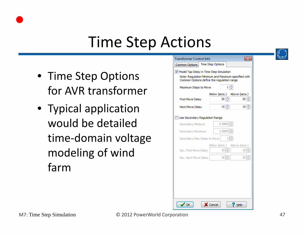
• Time Step Options for AVR transformer
• Typical application would be detailed time‐domain voltage modeling of wind farm
47© 2012 PowerWorld CorporationM7: Time Step Simulation

Custom Inputs
• Custom inputs allow
Custom Inputs
Custom inputs allow specification of more detailedmore detailed parameters in the time domain fortime domain for several object types
• Example: generator• Example: generator voltage setpoint
48© 2012 PowerWorld CorporationM7: Time Step Simulation

What is Saved in the TSB File?
• Because the amount of time information
What is Saved in the .TSB File?
generated in the Time Step Simulation may be significant, a binary file is used to store it. This is called the Time Series Binary ( TSB) filecalled the Time Series Binary (.TSB) file.
• This file will save:– Input DataInput Data– Scheduled Input Data– Custom Inputs– Result Definitions– ResultsTime Simulation Options (defined in the Options page)
49© 2012 PowerWorld CorporationM7: Time Step Simulation
– Time Simulation Options (defined in the Options page)

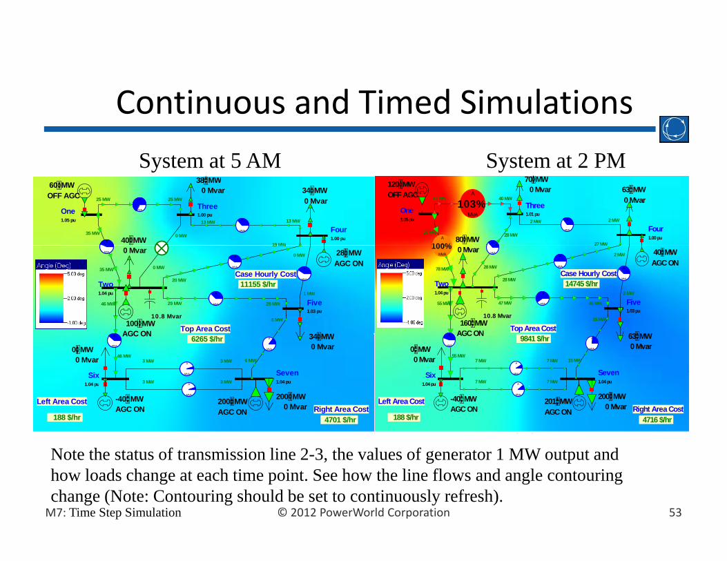
Continuous and Timed Simulations
• By default, when you hit the Do Run button, each
Continuous and Timed Simulations
y , y ,time step is solved immediately after the previous one. This is called a Continuous Simulation.
h h h d h l• On the other hand, the Time Step Simulation can mimic a solution in actual time by specifying a time scale. This is called a Timed Simulation.time scale. This is called a Timed Simulation.
• The Timed Simulation allows you to visualize the solutions on oneline diagrams as a movie. – You can see how time point and scheduled input data are applied and their effect on the system.
– You can also contour and animate
50© 2012 PowerWorld CorporationM7: Time Step Simulation
You can also contour and animate.
Continuous and Timed Simulations
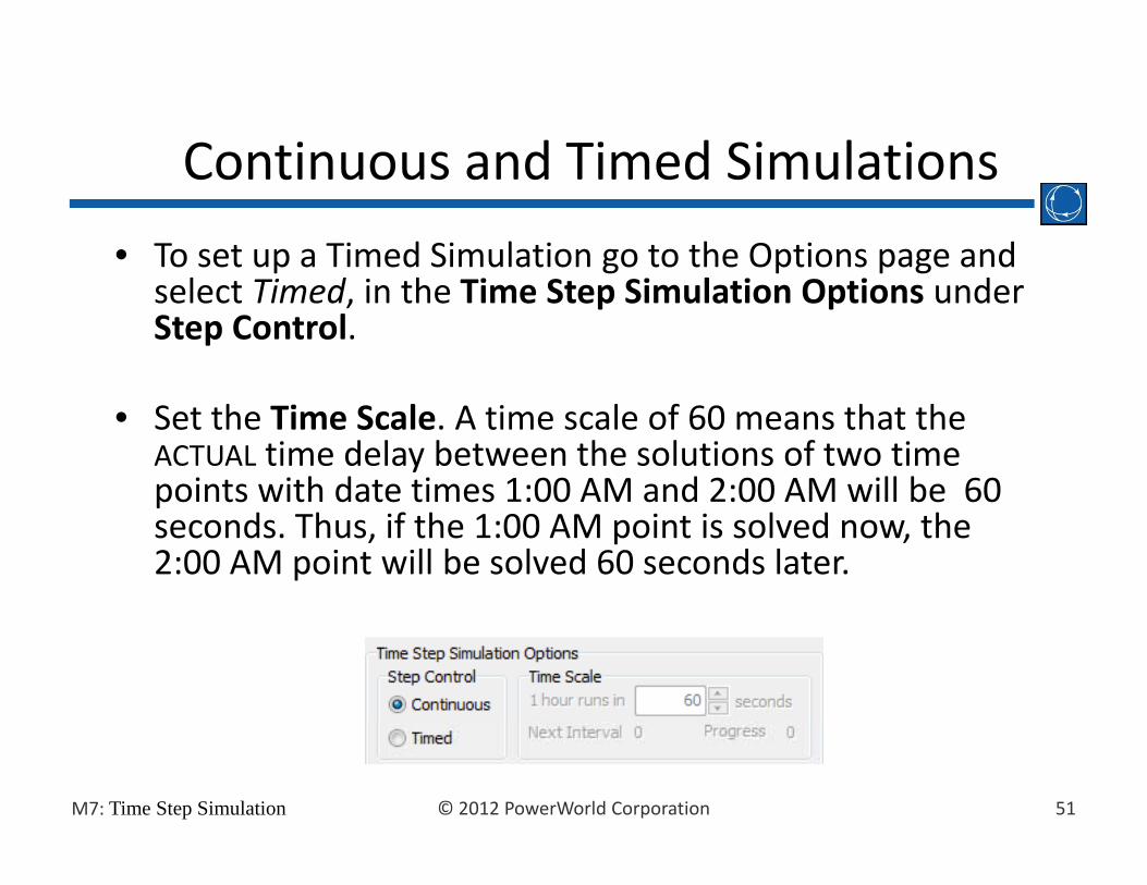
• To set up a Timed Simulation go to the Options page and
Continuous and Timed Simulations
select Timed, in the Time Step Simulation Options under Step Control.
• Set the Time Scale. A time scale of 60 means that the ACTUAL time delay between the solutions of two time points with date times 1:00 AM and 2:00 AM will be 60points with date times 1:00 AM and 2:00 AM will be 60 seconds. Thus, if the 1:00 AM point is solved now, the 2:00 AM point will be solved 60 seconds later.
51© 2012 PowerWorld CorporationM7: Time Step Simulation
Continuous and Timed Simulations
Example
Continuous and Timed Simulations
Example• Let us set the simulation to be Step Control = Timed, and
set a Time Scale of 5 (1 hour runs in 5 seconds of actual time).time).
• Move the Time Step Simulation dialog so you can see the oneline, but still have access to the control buttons.oneline, but still have access to the control buttons.
• Run the simulation by clicking Do Run
52© 2012 PowerWorld CorporationM7: Time Step Simulation
Continuous and Timed SimulationsContinuous and Timed Simulations
System at 5 AM System at 2 PM 60 MW 38 MW
0 Mvar 34 MW 0 Mvar
40 MW 1.00 pu
1.00 pu1.05 pu
A
A
MVA
A
MVA 35 MW
25 MW 25 MW
13 MW 13 MW
0 MW
19 MW
OFF AGC
One Three
Four
120 MW 70 MW 0 Mvar 63 MW
0 Mvar
80 MW 1.00 pu
1.01 pu1.05 pu
A
A
MVA 79 MW
41 MW 40 MW
2 MW 2 MW
28 MW
27MW
OFF AGC
One Three
Four
100%A
103%A
MVA
0 Mvar
1.03 pu
1.04 pu A
MVA
MVA
A
MVA A
MVA
35 MW 0 MW
29 MW 29 MW
19 MW
20 MW
1 MW
46 MW
28 MWAGC ON
Case Hourly Cost 11155 $/hr Two
Five
0 MW
10 8 Mvar
0 Mvar
1.03 pu
1.04 pu A
MVA
MVAA
MVA A
MVA
78 MW 28 MW
47 MW 46 MW
27 MW
28 MW
2 MW
55 MW
40 MWAGC ON
Case Hourly Cost 14745 $/hr Two
Five
2 MW
10 8 Mvar
100%MVA
Top Area Cost100 MW 34 MW 0 Mvar
1.04 pu1.04 pu
A
MVA
A
MVA
A
MVA
6 MW
6 MW 3 MW 3 MW 46 MW
0 MW 0 Mvar
A 3 MW 3 MW
AGC ON 6265 $/hr
Six Seven
10.8 Mvar
Top Area Cost160 MW 63 MW 0 Mvar
1.04 pu1.04 pu
A
MVA
A
MVA
A
MVA
15 MW
15 MW 7 MW 7 MW 55 MW
0 MW 0 Mvar
A 7 MW 7 MW
AGC ON 9841 $/hr
Six Seven
10.8 Mvar
Left Area CostRight Area Cost
-40 MW 200 MW
p
200 MW 0 Mvar
MVA
AGC ON AGC ON 4701 $/hr 188 $/hr
Left Area CostRight Area Cost
-40 MW 201 MW 200 MW 0 Mvar
MVA
AGC ON AGC ON 4716 $/hr 188 $/hr
Note the status of transmission line 2-3 the values of generator 1 MW output and
53© 2012 PowerWorld CorporationM7: Time Step Simulation
Note the status of transmission line 2 3, the values of generator 1 MW output and how loads change at each time point. See how the line flows and angle contouring change (Note: Contouring should be set to continuously refresh).

Time Step Simulation Toolbar
• The time step simulation toolbar is visible when the
Time Step Simulation Toolbar
pdialog is open and time points have been defined.
• It allows you to control the simulation (continuous or timed) without using the time step simulation dialogtimed), without using the time step simulation dialog.
Last Timed/ContinuousSi l i
Time Scale usedPresent Time
Simulation Control
Result Status Progress Bar
Simulation used in Timed
Simulation
for Timed Simulation
Buttons
54© 2012 PowerWorld CorporationM7: Time Step Simulation

Time Step Simulation ToolbarTime Step Simulation Toolbar
Reset the Simulation
Pause a continuous or
timed simulation
S l th tPlay the Time
S l th Solve the next Time Point
yStep Simulation
in either continuous or
Solve the previous Time
Point
55© 2012 PowerWorld CorporationM7: Time Step Simulation
timed mode.
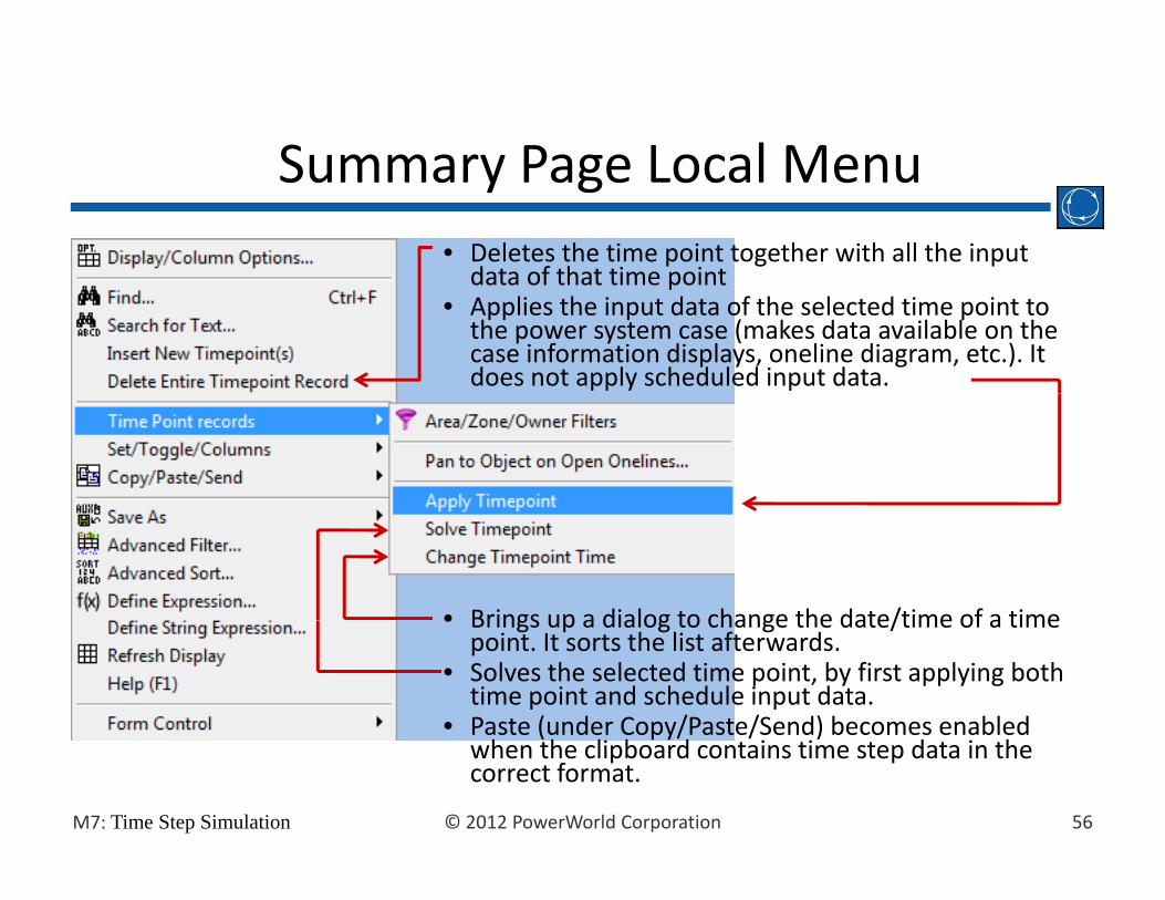
Summary Page Local Menu• Deletes the time point together with all the input data of that time point
Summary Page Local Menu
data of that time point• Applies the input data of the selected time point to the power system case (makes data available on the case information displays, oneline diagram, etc.). It does not apply scheduled input data.
• Brings up a dialog to change the date/time of a time• Brings up a dialog to change the date/time of a time point. It sorts the list afterwards.
• Solves the selected time point, by first applying both time point and schedule input data.
• Paste (under Copy/Paste/Send) becomes enabled
56© 2012 PowerWorld CorporationM7: Time Step Simulation
Paste (under Copy/Paste/Send) becomes enabled when the clipboard contains time step data in the correct format.
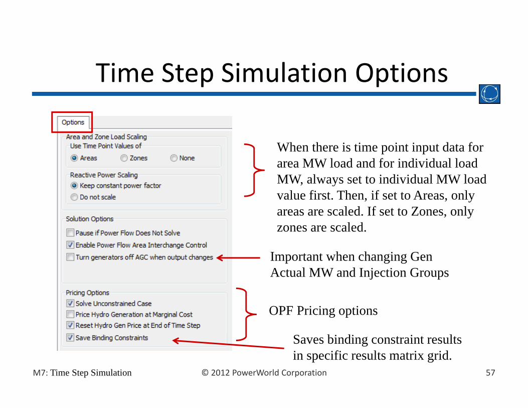
Time Step Simulation OptionsTime Step Simulation Options
When there is time point input data for area MW load and for individual load MW always set to individual MW loadMW, always set to individual MW load value first. Then, if set to Areas, only areas are scaled. If set to Zones, only zones are scaledzones are scaled.
Important when changing Gen Actual MW and Injection Groups
OPF Pricing options
57© 2012 PowerWorld CorporationM7: Time Step Simulation
Saves binding constraint results in specific results matrix grid.

Time Step Simulation OptionsTime Step Simulation Options
Ti S Si l i llTime Step Simulation allows you to either Apply and Solve or just Apply Data without solvingsolving.
Sometimes you want to test only time point or scheduleonly time point or schedule data
Loads the TSB automatically when the case is opened.
Wh i th TSB t
58© 2012 PowerWorld CorporationM7: Time Step Simulation
When saving the TSB, set automatically the Default tsb to be the current tsb.

Time Step Simulation OptionsTime Step Simulation Options
Options PageThe Time Step Simulation can contour oneline diagrams as the simulation takes place. It can also save a list of the resulting images as
Options Page
Bitmaps or JPGs.
59© 2012 PowerWorld CorporationM7: Time Step Simulation
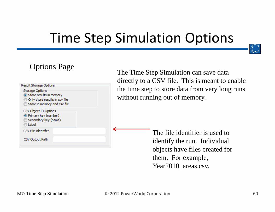
Time Step Simulation OptionsTime Step Simulation Options
Options PageThe Time Step Simulation can save data directly to a CSV file. This is meant to enable the time step to store data from very long runs
Options Page
without running out of memory.
The file identifier is used to identify the run. Individual objects have files created for them. For example, Year2010_areas.csv.
60© 2012 PowerWorld CorporationM7: Time Step Simulation
OPF and SCOPF Time Step Simulations
• Users of OPF and the SCOPF add‐ons can obtain
OPF and SCOPF Time Step Simulations
Users of OPF and the SCOPF add ons can obtain time point optimal power flow and security‐constrained optimal solutions by specifying these solution types for one or more time points in the Summary page.– Make sure you become familiar with Simulator OPF and SCOPF before running a Time Step Simulation with these options. p
61© 2012 PowerWorld CorporationM7: Time Step Simulation
OPF and SCOPF Time Step Simulations
Unconstrained OPF
OPF and SCOPF Time Step Simulations
• The Time Step Simulation will remove all the constraints that would normally act in the OPF and will optimize the system to find the minimum operating costsystem to find the minimum operating cost.
• Simulator will change the set points of the specified controls (generators and phase shifters) to minimize the
t f ll A d S A t t OPF AGC t lcost of all Areas and Super Areas set to OPF AGC control. • Besides the power flow solution options, the
Unconstrained OPF simulation will take all the options that have been defined for a regular OPF solution. Most of these options are defined in OPF Options and Results Dialog under the Add Ons ribbon tab.
62© 2012 PowerWorld CorporationM7: Time Step Simulation

OPF and SCOPF Time Step Simulations
OPF
OPF and SCOPF Time Step Simulations
OPF• The Time Step Simulation applies the time point and
schedule input data and optimizes the control areas set to OPF to minimize cost while enforcing normal operation constraints.– This includes: transmission line thermal limits, interface limits, , ,
generator control limits, and load control limits.
• The OPF algorithm detects the controls that need to be moved the constraints that are binding at the solutionmoved, the constraints that are binding at the solution point, and the unenforceable constraints, i.e., constraints that cannot be enforced with the available controls.
63© 2012 PowerWorld CorporationM7: Time Step Simulation
OPF and SCOPF Time Step Simulations
OPF
OPF and SCOPF Time Step Simulations
• Some of the quantities that are of interest in the solution of the OPF algorithm, are displayed in the Result: Constraints Pages:Constraints Pages:– Unconstrained Generator MW Output– Final generator MW Output
Change in Generator MW– Change in Generator MW– Locational Marginal Prices: These are displayed in the Hourly Final
Bus LMP Page. Average LMP prices and other LMP metrics are also available in the Results Page for Areas, Injection Groups,also available in the Results Page for Areas, Injection Groups, Super Areas, and Zones.
– Binding Constraints as well as Marginal Cost of Limit Enforcement for lines and interfaces.
64© 2012 PowerWorld CorporationM7: Time Step Simulation

OPF and SCOPF Time Step Simulations
SCOPF
OPF and SCOPF Time Step Simulations
• The SCOPF combines Simulator’s OPF with Contingency Analysis to optimize a system for minimum cost while enforcing both normalminimum cost while enforcing both normal operation and contingency constraints.
• The solution of an SCOPF Time Step Simulation depends on the options that have been set up for the following tools:– Power Flow– Optimal Power Flow– Contingency Analysis Security Constrained Optimal Power Flow
65© 2012 PowerWorld CorporationM7: Time Step Simulation
– Security Constrained Optimal Power Flow– Time Domain OPF Options

OPF and SCOPF Time Step Simulations
SCOPF
OPF and SCOPF Time Step Simulations
• At each time point, the SCOPF Time Step Simulation does the following:– Applies the input data and scheduled actions– Solves a power flowIf specified it solves an unconstrained OPF– If specified, it solves an unconstrained OPF
– Initializes the base case for the SCOPF by solving a power flow or an OPF
– Solves the contingencies for the initialized system state– Solves the SCOPF optimization problem– Displays the results in the matrix grids
66© 2012 PowerWorld CorporationM7: Time Step Simulation
– Displays the results in the matrix grids
OPF and SCOPF Time Step Simulations
SCOPF
OPF and SCOPF Time Step Simulations
• The SCOPF often requires significant computer resources mostly because of the need to solve a large number of contingencies and to calculate their sensitivities.
• The size of the problem also depends on the size of the system, number of constraints (monitored elements), and number of time points considered.
• A mechanism to speed up the computation of the PF/OPF/SCOPF Time Step Simulation is to use DC solutions in some of the internal routines:– AC or DC power flow– AC or DC contingency analysis. This one will produce the larger
time savings. – AC or DC SCOPF
67© 2012 PowerWorld CorporationM7: Time Step Simulation
– AC or DC SCOPF

OPF Pricing Options
• Different applications of the OPF/SCOPF require special
OPF Pricing Options
Different applications of the OPF/SCOPF require special pricing options.
• A method for congestion pricing consist of solving first the unconstrained case to determine unconstrained LMPsunconstrained case to determine unconstrained LMPs, and then solve the OPF or SCOPF. The difference between these two solutions correspond to the congestion cost or congestion component of the LMP for a given hourcongestion component of the LMP for a given hour.
Check this option to solve an i d OPF ( i lunconstrained OPF (equivalent
to economic dispatch) before solving the OPF or SCOPF for each time point
68© 2012 PowerWorld CorporationM7: Time Step Simulation
each time point.

OPF Pricing Options
• It is also customary in LMP k h d
OPF Pricing Options
markets to price hydro generation at a cost equal to the unconstrained LMP. Si l t ill i t ll• Simulator will internally modify the cost curve of the hydro generation to match the unconstrained • Check this option to reset match the unconstrained LMP obtained during the initial unconstrained simulation. It will then
the cost curve of hydro generation to the original cost after each time step.U h k hi isolve the constrained
optimization problem using this cost for the hydro
it
• Uncheck this option to explore how Simulator changes the hydro cost to the unconstrained marginal
69© 2012 PowerWorld CorporationM7: Time Step Simulation
units. the unconstrained marginal price.
OPF Pricing Options
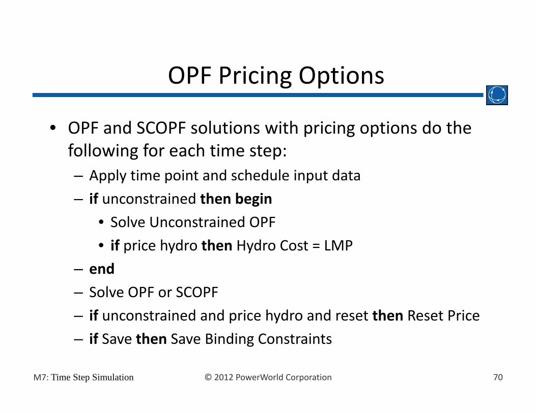
• OPF and SCOPF solutions with pricing options do the
OPF Pricing Options
• OPF and SCOPF solutions with pricing options do the following for each time step:– Apply time point and schedule input datapp y p p
– if unconstrained then begin
• Solve Unconstrained OPF
• if price hydro then Hydro Cost = LMP
– end
– Solve OPF or SCOPF
– if unconstrained and price hydro and reset then Reset Price
if Save then Save Binding Constraints
70© 2012 PowerWorld CorporationM7: Time Step Simulation
– if Save then Save Binding Constraints
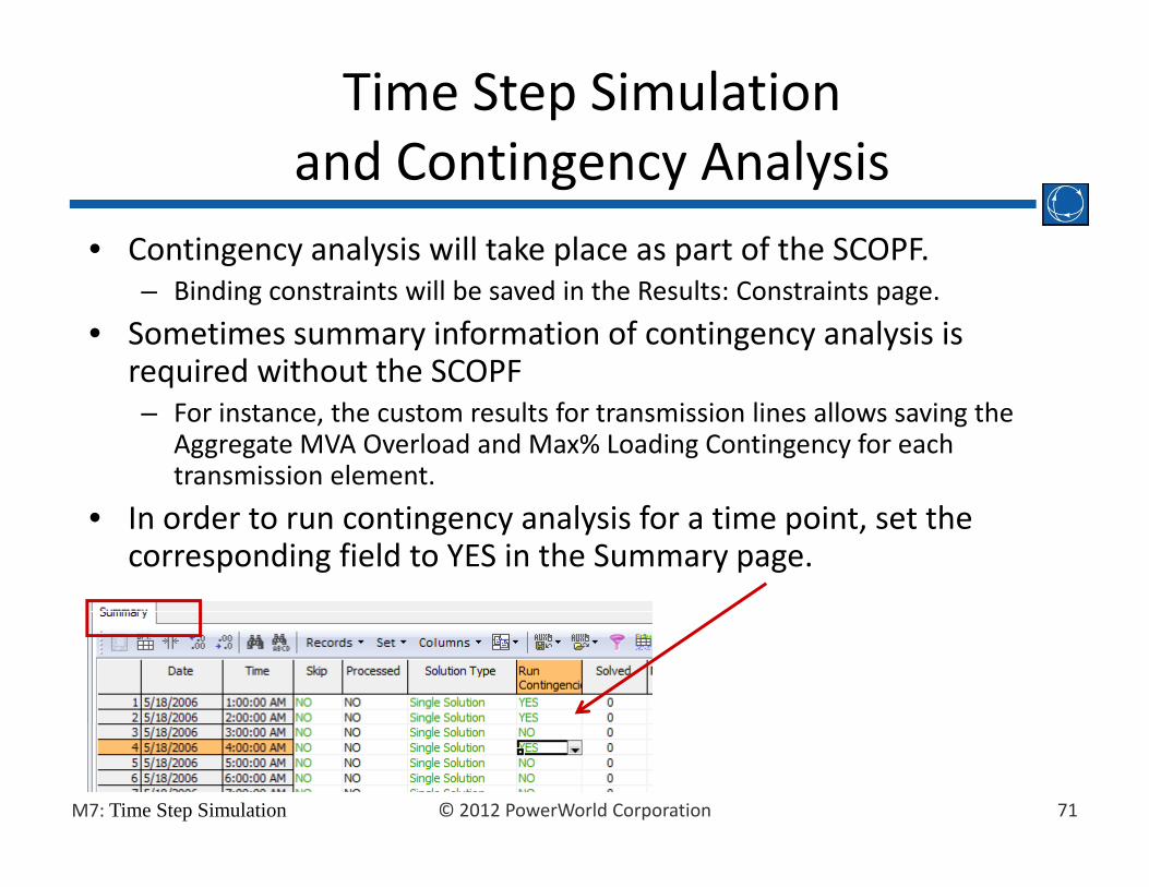
Time Step Simulation and Contingency Analysis
• Contingency analysis will take place as part of the SCOPF.
and Contingency Analysis
– Binding constraints will be saved in the Results: Constraints page.
• Sometimes summary information of contingency analysis is required without the SCOPFq– For instance, the custom results for transmission lines allows saving the
Aggregate MVA Overload and Max% Loading Contingency for each transmission element.
• In order to run contingency analysis for a time point, set the corresponding field to YES in the Summary page.
71© 2012 PowerWorld CorporationM7: Time Step Simulation

Blank Page