m OI m T COPY: (WLIL-2) n AFB, z c · FOR VIDEO SIGNALS bY ... The ten Tiros television cloud pictures used in the study ... A detailed explanation of how the technique is applied

---?- NASA TN /- D-3395 c k /

NASA TECHNICAL NOTE

m OI m T AFWL (WLIL-2) n

LOAN COPY: RETURN 7 0

KIRTLAND AFB, N MEX z c 4 v) 4 z

ADAPTIVE DATA COMPRESSION FOR VIDEO SIGNALS

bY A. V. Bulukrishnun University of CuZzj$ornia at Los Angeles and R. L. Kat2 und R. A. Stampfl Goddurd Space F&gh Center

N A T I O N A L AERONAUTICS A N D SPACE A D M I N I S T R A T I O N WASHINGTON, D. C. A P R I L 19i6

https://ntrs.nasa.gov/search.jsp?R=19660013631 2018-08-29T09:55:59+00:00Z

NASA TN D-3395


By A. V. Balakrishnan

University of California at Los Angeles Los Angeles ,. Calif.

R. L. Kutz and R. A. Stampfl

Goddard Space Flight Center Greenbelt , Md.

NATIONAL AERONAUTICS AND SPACE ADMINISTRATION

For sale by the Clearinghouse for Federal Scientific and Technical Information Springfield, Virginia 22151 - Price $2.00

ABSTRACT

The properties of adaptive predictors a r e discussed and a brief derivation of the prediction mathematics is given. The ten Tiros television cloud pictures used in the study are described and the method used to display them on the Stromberg Carlson 4020 microfilm recorder is discussed. A detailed explanation of how the technique is applied to televisionpictures and how it is programed on the computer is given. The result of the compression on the quality of the TV pictures is discussed and is shown by the pictures displayed herein.

ii

CONTENTS

Abstract . . . . . . . . . . . . . . . . . . . . . . . . . . . . . .

INTRODUCTION . . . . . . . . . . . . . . . . . . . . . . . .

PROPERTIES OF ADAPTIVE PREDICTORS . . . . .

THEORY OF ADAPTIVE COMPRESSION SYSTEM . .

TIROS VIDEO DATA . . . . . . . . . . . . . . . . . . . . .

COMPUTER IMPLEMENTATION . . . . . . . . . . . . .

DISCUSSION OF RESULTS . . . . . . . . . . . . . . . . .

CONCLUSIONS . . . . . . . . . . . . . . . . . . . . . . . . .

ACKNOWLEDGMENTS . . . . . . . . . . . . . . . . . . . .

References . . . . . . . . . . . . . . . . . . . . . . . . . . . .

Appendix A-Symbols . . . . . . . . . . . . . . . . . . . . .

ii

1

2

3

8

11

18

22

22

22

43

iii


by A. V. Balakrishnan

University of Cali fovnia

R. L. Kutz and R. A. Stampfl Goddard Space Flight Center

INTRODUCTION

The spin-stabilized Tiros and Tos weather satellites produce, along with other data, large quantities of television pictures. The two television cameras on board can televise directly when within communication range of a ground station, and, more importantly, they can store 32 TV frames per camera on magnetic tape and transmit this information when an appropriate ground command is given. A 62.5-kc video bandwidth is employed for the transmission of 500 line frames, each with a frame duration of 2 seconds. The gray scale quality of the pictures varies between 5 and 10 levels as a function of camera tube life and telemetry performance; 6 levels can be considered an average quality value.

4J

When pictures a r e received at ground stations, a composite mosaic consisting of overlapping individual frames is prepared from the 32 picture ser ies with the help of the satellite attitude data available from other data channels. Meteorologists at the receiving sites transpose the meteorological information content onto weather maps by visual inspection. Cloudiness of the area viewed, types of clouds, and interpretive results such as fronts and storm centers a re all noted on maps; the results a r e conventional nephanalyses. These nephanalyses a r e transmitted via facsimile links to forecasting centers o r a r e translated into teletype messages for distribution. A sample of a mosaic and the corresponding nephanalysis and teletype message a re given in Figure 1.

The glaring difference between the number of data points contained in 32 pictures o r in a prepared mosaic and the true meteorological information content of the mosaic s t resses the need for research aimed at practical data compression methods. Fully operational satellites delivering data continuously by covering the entire earth every 12 hours will benefit even more from the results of such studies. The present paper reports on the method employed to compress video data by applying adaptive prediction of the kind first reported by Balakrishnan (Reference 1) to a sample of ten Tiros cloud pictures. The choice of this rather elaborate method using computer implementation rather than another approach was made after a brief investigation showed that trivial approaches will yield only meager data compression. Delta modulation, a simple technique in which the amplitude difference between adjacent samples is transmitted and the sampling rate is chosen such that no more than 1 quantum step difference is expected, is objectionable because resolution is lost on high-contrast transitions. An implementation of the delta modulation method has

1

SAMPLE MISCELLANEOUS SATELLITE BULLETIN

22,41252 E 17.N, 57.5W, STAGE X, DIA 5, BANDS 2, TROPICAL STORM BEULAH, EYE NOT VISIBLE, STORM CENTER LOCATED WITHIN BROAD CLOUD BAND TIP AT 18N, 58W.

25/1315Z AUG GWBC

AL STORM BEULAH

E' 40" N-

COAST SOUTH AMERICA

-0" N

'20" N MAX. -WINDS 60KTS t

-60' N

55 'N

N

Figure 1-Sample of a mosaic and the corresponding nephanalysis and teletype message.

the most attractive circuitry because of its simplicity but visual inspection of cloud pictures con- f i rms objectionable loss in picture resolution. Even though pictures can be transmitted by a four- bit code because of the limited number of gray levels, the total number of bits per frame is seldom reduced more than two to one when delta modulation is used. Run-length coding, a technique where the number of consecutive elements with constant attributes a re counted, has also been investigated; there were no conclusive results but the need was shown for computer simulation s o that a variety of methods can be tried with minimum investment.

PROPERTIES OF ADAPTIVE PREDICTORS

The technique used in this study is adaptive and has been presented rigorously in the literature (see Reference l), so an analysis of the basic features of the system shall suffice. An adaptive

2

system is distinguished primarily by an explicit or implicit learning mode; 'however, to be truly adaptive the system must have other features as well.

At this point it is well to present some definitions: Adabtive: Implies modification to meet new conditions. Adjusting: Implies a bringing into as exact or close a correspondence as exists between the parts of a mechanism, but suggests more tact or more ingenuity in the agent. "Adjust- ing" appears to be a more exact description of the system than "adaptive," but the word "adaptive" has become general usage. Actually, i t is impossible to draw a sharp distinction between what is adaptive and what is not. The word adaptive does signify something more than a self-adjusting mechanism (such as, say, an AGC o r AFC system where there a r e no conditions not envisaged at the time of design). Without getting involved in semantics, one can say that an adaptive system is one which monitors its own performance; the system learns what the new conditions a r e and changes its structure accordingly. (In a biological system where the adaptivity is more easily described, the performance criterion would be self-preservation.)

In a comniunication system the new conditions consist of parameters changing in some a PYiori unknowable fashion. These parameters have to be learned o r measured and appropriate changes must be made in the system to maintain a prescribed level of fidelity, or some other chosen criteria. A simple example is the usual Shannon-Fano noiseless coding for minimal length, which requires complete specification of the message probabilities. In many cases (strictly speaking, in all cases) these probabilities a r e unknown and have to be measured. Moreover, if the probabilities a r e also subject to change, we need a learning phase, whether it is or is not separate from the coding phase. One cannot call such a system "adaptive" since there is no monitoring of performance involved. In a two-way o r feedback communication system (such as a data transmission system) the receiver monitors quality of performance (with an error-detecting code) and the transmitter adjusts by reducing the transmission rate or stopping transmission altogether. There is no learning involved here so this system is not quite adaptive in the sense in which we construe it. The learning phase is triggered by a degradation in performance. Now a radar system which simply measures, say, the clutter o r reverberation parameters and then changes the detection circuitry parameters is not quite adaptive since there is not a self-monitoring criterion. If, for example, the transmission system learns or measures channel characteristics and changes its mode of transmission accordingly to restore the performance quality, it would be a truly adaptive system.

Actually, the term "adaptive" is beginning to be used whenever there is a learning o r measure- ment feature (implicit or explicit) even if there is no self-monitoring. (The terms self-regulating and self-adjusting are used for systems with the monitoring feature but with no learning feature.)

THEORY OF ADAPTIVE COMPRESSION SYSTEM

Note that the compression system is truly adaptive in the sense that it features a self-monitoring function in addition to the learning and adjusting functions.

Let x( t ) represent a continuous o r discrete parameter source. It is customary to assume that x(t) can then be regarded (at least for analytical purposes) as a stochastic process. If the

3

time parameter t is continuous, it is often possible to assume that

x( t ) = rB e2nift d$( f )

in a suitable sense (that is, depending on whether we adopt the stochastic or nonstochastic view- point) for sufficiently large values of B, the bandwidth. By use of the well known "sampling principle" one can then represent the continuous waveform using periodic samples taken at t n / 2 ~ .

In most communication systems using sampled data of this kind, the sampling rate is determined by the nominal highest or cut-off frequency B expected in the data. However, in the case of many kinds of data-such as space-telemetry data-the actual cut-off frequency will be much smaller for most of the time, so that there is no need to sample at the nominal rate of 2 ~ . In other words, it is possible to "compress" the data sampling rate or channel bandwidth.

A method of achieving such compression in PCM systems is to exploit the redundancy or predictability of the data. Thus, we employ a "predicator" at the transmitter which predicts the data at time t + A based on the past data up to time t . The actual value sampled is then compared with the predicted value. If the difference exceeds (in absolute value) a preset threshold, then the actual sample is transmitted. If it is below the threshold, a prearranged code word using say, one digit is transmitted instead of the m digits, thus reducing the number of digits transmitted per second. A comma-free code may be used to sor t out the two kinds of words unambiguously. The adaptive or learning feature comes in the predictor mechanism. The predictor is not updated until i ts threshold is exceeded; this exhibits the self-monitoring feature. The predictor itself is based on a learning phase, and the prediction operator is adjusted accordingly. For details on the predictor itself see Reference 1. The significance of the adaptive prediction feature lies in the fact that no a pviom' statistics o r other assumptions concerning the data a r e required, and, in particular, i t is realized that there may be periods in the data where prediction (to the q.Jality set) may not be possible.

The basic prediction philosophy may be indicated briefly. We a r e given a waveform of duration T (i.e., T is a function x ( t ) , 0 < t 5 T ) and we a r e required to predict the value at time T + A . Any prediction operation is to be based on the data alone, no additional a priori knowledge being available. This is, of course, an ancient problem, but here we wish to treat it strictly in the telemetry data processing context and to note two major methods of dealing with it. One, which may be considered the numerical-analysis method, consists in assuming that certainly any physically realized waveform must be analytic and can thus be approximated by polynomials. The data may thus be "fitted" to a polynomial of high enough degree and we then simply use this polynomial to predict the future values. The other and more recent method is the statistical view in which we assume (perhaps with good reason) that the data are finite samples of a stationary stochastic process; the process' average properties, such as moments and/or distributions, are known or calculable from the data. For a process of given description we can apply the well-developed mean-square prediction theory. Perhaps the main advantage of this method is that it gives u s a

4

quantitative, albeit theoretical, notion of the e r ro r in prediction. The problem of measuring the average statistics from a finite sample can be quite delicate, however. In the polynomial fitting method, the interpretation of the prediction error-which is, after all, the crucial point-is more nebulous and is bound up with the degree polynomial to be used and the portion of the data to be fitted. Moreover, as ordinarily used, the fitting operations on the data a r e linear.

We adopt a rationale for prediction which is free from a Priori assumptions concerning the "model." In a general sense what is involved in both the above methods is, first, "model-making" consistent with the data and, second, using the numbers derived therefrom to perform some optimal operations. If an understanding of the mechanism generating the model is desired, the first step is essential. If prediction is the object, it is possible to proceed directly (and hence more optimally) to the best prediction without the intermediate step of model-making. It may be, of course, that several approaches lead to the same operations on the data; however, the present method offers some practical advantages and it is desirable to use the approach that requires the fewest prior assumptions.

We note first that any prediction is an operation or operator on part of the data, and in our case, the finite part is all that is available. The main point of departure in our view is that i f we have a prediction operator, which based on all the available input data, functions optimally in the immediate past of the point where the prediction is required, this is all that we can ask for mean- ingfully as a solution to the prediction problem. Thus, the only basis on which we can a pviori judge any prediction method is to "back off" slightly from the present and compare the actual available data with the predicted value using the given prediction operator.

Let us see how this can be formulated analytically. Let the total available data be described as a function X( t ), where 0 5 t 5 T , and let the prediction of the value at T + A , (here A > 0 , being a small fraction of T) be required. Let u s next consider the data in the interval 0 < t < ( T - A ) . If for any t o in this interval we should choose to make a prediction of the function value A ahead from the past values up to to and denote the predicted value by

x* ( to + A )

we can explicitly observe the e r ro r

x* ( to +A) - x ( t o +A) '

Let us next note that the general prediction operator will be a function of a finite segment of the past. Let u s denote the length of this segment by M . Then, of course,

x * ( t o + A) 0 { x ( c ) : t o - M < m < t } ,

where o represents the prediction operator.

Next w e have to specify the e r r o r criterion. We choose the mean square e r r o r because it is both simpler analytically and almost universally used and so comparison with other methods is possible. The kind of solution presented is definitely not analytic, but, rather, is based on successive approximation so other measures of e r ro r can be used at the r isk of greater complexity. As far as the rationale of the method is concerned, this is largely a matter of detail rather than principle. We can thus use to determine optimality:

T- A

[ x * ( t t A ) - x ( t t A)]’ d t = E *

T-n-L t M

where M <L, and we proceed on the basis that the operator o is best which minimizes Equation 3. W e can, of course, generalize Equation 3 as

(3)

where M is the domain of 0 for a prediction at t o , p( t ) is a positive weight function, and the function c is, say, a symmetric positive cost function (a complete list of symbols is given as Appendix A). Before we consider the problem of determining the optimal operator 0, let us note an important consistency principle. Suppose the data a r e regarded as one long sample of an ergodic process. Then Equation 3 yields exactly the optimal operator in the statistical sense. However, we have not needed to make any suck &tion concerning the data; nor have we had to compute average statistics first. The point is that while the data may not be enough for determining, let u s say, the spectrum, it may be quite adequate for the prediction itself. Unlike the polynomial fitting, the operations on the data can be as nonlinear as necessary, and at the same time Equation 3 normalized to

yields a quantitative measure of the prediction e r r o r on which to judge how good the prediction will be. For actual methods of determination of the optimum predictor see Reference 1.

So far we have determined the optimal adaptive structure, but there still remains the problem of evaluating the system. For instance, it is natural to ask what is the average amount of compression it is possible to obtain in this way. Here we have to postulate some structure for the data source and then calculate the resulting compression using the adaptive system. We shall now briefly indicate what an analysis of this type involves. Not to complicate the analysis unduly, let u s consider the prediction operation in the transmitter based only on the actual samples. Let us denote the data samples by xn . We assume that the data can be taken as a stationary stochastic process. We may further assume that the process is Gaussian since the maximum prediction e r ro r

(and hence the minimum compression) occurs in this case because the prediction operation includes only the linear case. Let us consider the case where the adaptive predictor is also constrained to be linear. In this case the optimal filter weights aj are determined by minimizing

L - M n=-Lt1 tM

where the past available data consist of L samples and the prediction is based on M samples. We are, of course, considering the analog method above. The corresponding (squared) e r ro r is then

The transmission is based on Equation 7 exceeding a thresholdT,. Hence, what we want first is to determine the statistics of Equation 7. We note first that the optimal {%} that minimizes expression (6) will satisfy:

x n Xn-k = 2 f: a j xn-, , k 1, . * . , M . n=-L+1 +M 1 - 1 n=-L+ItM

Let Y be the vector

x n - L t 1 + MI . . . [ x n , X n - 1 '

Then the minimum of expression 6 becomes

1 % + I , _ _ ~ L - M DM

where DM+I is the determinant of the M + 1 by M + 1 matrix with entries

Y i . Y i , i , j = 0, -1, * * . , -M

and Dm is the determinant of the M-by-M matrix with entries

Yi . Yj, i , j = -1, -2, * - - , -M

On the other hand, we are interested in the e r r o r (7), which is

- €02 [M; L] -

where Ddt1 has first row

and is otherwise the same as DMtl. Our first interest is in the statistics of Equation 8. We need to know

which is the probability of exceedence of the threshold and relates directly to the attainable compression. Actually Equation 8 determines only the "open-loop" error , and to evaluate the complete system we have to consider the "closed-loop" operation where actual samples a r e replaced by predicted samples when the former fall within the set threshold.

Equally important, we need to know what the quality of the compressed data will be. One may, for instance, use the cross-correlation coefficient or another equivalent quantitative index and evaluate this as a function of T,, M, and L. A complete system evaluation requires that channel noise be also taken into account. Such an analytic evaluation is necessary to provide a logical basis for choosing optimum design parameters. Indeed, if the channeI noise characteristics a re known, appropriate coding or signal selection has to be considered in arriving at the total compression possible.

TIROS VIDEO D A T A

Many of the thoughts expressed here go beyond the scope of the present investigation, an application to Tiros television. It is reasonable to expect remarkable future progress in applications of the theory when one considers the recent progress in the field.

Application of the technique to Tiros TV data requires appropriate conversion of the original analog magnetic tapes to computer compatible tapes. This data compression technique was chosen for investigation instead of another because of the high expectation that other techniques could do no better and because this technique permits comparison with a nearly ideal situation. In applying the method, the three picture elements preceding the data point to be,predicted a r e usually used. They are called the memory M in this report, A weighting function is derived from a chosen sample of L picture elements, here referred to as the learning period (see Figure 2). The learning period L = 20 was used for many of the computer runs; however, other intervals can be chosen and data compression has been attempted with M = 3 and L = 20, M = 0 and L = 20, and M = 0 and L = 1.

Video data for this study were obtained from the standard Tiros FM subcarrier modulated magnetic tapes; the data were converted by use of the A/D converter to six-bit characters and were recorded on magnetic tape at a density of 556 characters per inch in one physical record of 40,000 words with 36 bits per word.

8

~ TV elements of learning set

memory

set

of I ea m i ng 1

Figure 2-Relation of learning and memory sets.

The video input to the A/D converter included horizontal sync pulses to provide line sync in the conventional analog Tiros display system. A program for the IBM 7094 computer read each 40,000-word record in two passes, since the core capacity is only 32,000 words, found line sync, and reformatted the data into 24 records of 20 lines each. Each line of TV data now contained 468 elements with 480 lines in each TV cloud picture; this was a reasonably good match to the 500- element, 500-line analog original pictures. The reformatting and sync program for the 7094 did not find the start of each TV line with perfect consistency and for this reason some of the TV lines were registered incorrectly, as is evident by inspection of the TV cloud pictures used in the study. The dynamic range of the analog data entering the A/D converter was adjusted so that it was smaller than a six-bit code would permit. A tolerance was allowed at the minimum and maximum amplitudes of the analog video data so that only approximately 32 of the possible 64 amplitude levels were used in the converter. The TV data used in this study should therefore be considered five- bit data.

A number of typical Tiros pictures (Figures 6 to 15) have been selected; these pictures show a variety of cloud patterns so that individual interpretation after processing permits general judg- ment as to acceptable quality. Pictures from both Tiros operating modes have been analyzed, that is, those recorded in the satellite and played back later and also those transmitted directly when within communication range. The latter pictures are preferred because they show slightly better quality than do the taped ones.

The first four pictures (Figures 6(a) to 15(a)) are part of a direct camera sequence of Tiros III, orbit 4, when the satellite was moving east-south-east over the central U.S. They were taken on July 12, 1961, and the picture principal point, which is near the cross fiducial mark, lies in the SW corner of Minnesota in Figure 6(a) and in North Central Iowa in Figure 9(a). The data log indicates for this orbit that the satellite camera was looking in a northwesterly direction. Because of the spin of the satellite the north direction may be different for each picture. Visualization of the geometry is simplified by the fact that the spin axis was practically in the orbital plane on the first day when orbit 4 occurred. Heavy cloud masses in a very distinct pattern can be seen, as well as large clear areas and regions of scattered overcast. The brightness levels viewed by Tiros cover the entire range of cloud cover intensities from black to full brightness.

9

The next two pictures (Figures lO(a) and ll(a)) were obtained again from Tiros 111 but are in the tape mode and are successive frames from orbit 102. The principal point lies near the Ivory Coast of Africa in Figure lO(a) and Liberia, Africa, in Figure l l(a). They were taken approximately 1 week after the preceding series. These two pictures were selected because of the random nature of the cloud pattern. It is also interesting to note the strong effect of viewing angle under the same sun illumination by comparing the two adjacent frames. The next picture processed (Figure 12(a)) was taken by Tiros V on orbit 3143 in the direct mode after 219 days orbital camera life in late January 1963. It shows distinct streakiness in the clouds grouped into two large sections in the picture. The clear long banded areas a r e also distinct features.

The remaining three pictures included in this study (Figures 13(a) to 15(a)) were taken by Tiros VI in December 1962, September 1962, and May 1963, respectively. Figure 13(a), in the direct mode, shows a tropical storm under oblique view in the Atlantic off the coast of Miami; Figure 14(a), in the tape mode, shows a large cloud area over the Atlantic located south of Green- land; and Figure 15(a), in the tape mode, shows a mature tropical storm located in the Atlantic northeast of the Bermuda Islands.

The digitized pictures (Figures 6(b) to 15(b)) were reproduced as four-bit encoded signals because of the limited dynamic range of the Vidicon and the display. As was to be expected, no noticeable difference can be detected. Reproduction of the pictures was accomplished on a Strom- berg Carlson 4020 microfilm recorder. The input for this machine came from digital magnetic tape produced as an output of the data-compression programs. This machine has the capability of plotting symbols on a 1024 X 1024 grid with 16 different intensities including the zero o r no-plot intensity (see the scale at the bottoms of the figures). The plotting symbol used here was the dot. This symbol requires the least a r ea and does not overlap if odd rows and columns in the plotting grid a r e skipped. Thus, a 512 X 512 grid is available for picture plotting, gray scale plotting, and the printing of identification marks. The fifteen intensities which cause darkening of the paper a re produced by unblanking the exposure beam from one to fifteen counts, in correspondence with a four-bit control word. This method of exposure does not produce a gray scale which is linear to the eye.

In order to produce a gray scale which would appear approximately linear, a power rule for the exposure time was used. Although a standard gray wedge has intensities which change by a ratio of fi, a smaller change is still easily seen by the eye. An exposure ratio of 1.25:l was used here. In this manner a gray wedge was produced by starting with an exposure time of four counts and increasing the exposure time in steps corresponding to a ratio of 1.25:l until 91 counts were reached. This provides fifteen gray steps with differences in intensity which look equal to the eye. The SC-4020 uses a lens with a variable diaphragm controlled by the f setting to project the CRT image onto the display medium. It was determined by eye that f16 produced the same shade change between the background and the first step, which is a count of four, as the shade change produced by the 1.25 exposure time rule. Another factor controlling the choice of the f setting was that below f16 the range of the display medium would have limited the gray scale on the dark end.

10

Sixteen levels of gray changing in steps which look equal to the eye were produced in this manner to correspond to four-bit data. When five-bit data were displayed the least significant bit was dropped. The pictures which appear in this report probably will have lost some of the linearity of the gray scale because of the reproduction process but the overall quality should not be degraded because of the large number of gray shades present. The difference in quality between the analog original copies and the digitally reproduced versions is quite pronounced and merely a consequence of the particular properties of the equipment used. Better reproduction techniques can readily be designed when specific methods a r e to be implemented. Contouring due to the finite number of quantum steps is visible but less objectionable than the appearance of the reproduction process. Superposition of random noise can eliminate the contouring and thereby cope with this psychological objection.

COMPUTER IMPLEMENTATION

In the practical implementation of the method previously described, it is necessary to generate a set of weights which will produce the best estimate of the most future data samples when operating on past data samples. In an actual telemetry system only the unpredictable elements need to be transmitted. This condition of unpredictability is said to exist when the absolute difference between a prediction and the data element being predicted exceeds a preset, chosen threshold T,.

In such a telemetry system, which will eventually be designed, the receiver and transmitter will use the same set of weights and will operate on identical data elements so they can produce the same estimates of future points. The weights could also be calculated at the transmitter and telemetered to the receiver, but i t seems wiser to send data rather than weights which a r e derived from the data. It might also take longer to transmit the weights than to transmit the data since the weights may have to be approximated to many places in order to get satisfactory results.

Here the set of weights is found from a set of TV elements called the learning set. Let the number of elements in the learning set be denoted by L . The first learning set is taken from the beginning of the first TV line. The first TV line has been taken here to be the top of the picture and its beginning is on the left-hand side so that the picture is scanned left to right and top to bottom. Each succeeding learning set is taken to begin at those multiples of ~ / 2 from the beginning of each line at which new weights a r e desired. A new set of weights is needed when it is found that, on the average, the old se t of weights is no longer producing satisfactory estimates. The r m s prediction e r r o r is checked every L/2 elements against a threshold T, to determine when new weights a re required. Threshold T, has previously been adjusted so that if T, is exceeded, many of the estimates of the last L/2 elements predicted would have exceeded T, . Those estimates which exceed T, are discarded and for the corresponding unpredictable picture element an original data element is substituted for transmission. Therefore, each interval of L/2 over which prediction has been attempted will contain original data elements and/or elements estimated by the predictor depending on whether T, had or had not been exceeded, respectively. Each time T, is exceeded L/2 elements from the last prediction interval and the succeeding L/2 original data elements are used for the required learning set. This choice is made to minimize the requirement

11

fo r transmission of actual data elements since only ~ / 2 (not L ) original data elements must be transmitted immediately following the exceedence of threshold T,.

The generation of new weights in an actual transmission system is costly and is thus to be avoided. Two measures have been taken to avoid unnecessary weight generation and a fortiori data transmission. First, at the beginning of each line, starting with the second line, the weights from the beginning of the preceding line are used; thus some advantage is taken of line-to-line correlation. The last set of weights calculated within 2~ elements from the beginning of a line are the weights used for the beginning of the next line. The same set of weights is used to start all successive lines until T, is exceeded within 2L from the s tar t of some future line; at this point the cycle starts again. Original TV data elements need be transmitted only at the start of each line in such quantity that the weights can be used to make the first estimate. Second, as one approaches the end of each TV line a new set of weights becomes less important since few elements remain to be estimated. Therefore, when only L or less elements remain to be estimated near the end of a TV line T, is ignored and the prediction process still using TI continues to the end of the line. Notice that the only place L original data elements are transmitted and used in the learning set, a priovi, is at the beginning of the first line of each TV picture.

The method of producing the weights was to minimize the mean square estimation e r r o r over the learning set. A number of tests made in the "open loop" mode showed that satisfactory results can be obtained with the chosen values of M and L.

The set of elements upon which the weights operate to produce an estimate is called the memory and consists of the M picture elements immediately preceding the element to be estimated. According to the theory each estimate not only depends on the M elements of the memory but also on a constant K . It is convenient to denote W as the weight vector containing the set of M t 1 weights; then the number of W's in the set of weights is M + 1 corresponding to K and the M elements in the memory. The weight vector W is the unknown to be found by using the learning set. This is accomplished by solving the matrix equation sw = P, where s is a matrix that has its rows made up of a memory set plus K , and P is a column vector of TV elements to be estimated from the corresponding row of the memory matrix S.

For example, let x,, X n + l , X n + , , , XntL-l be a learning set of elements for some n = 1, 2 , ... , 468 - (3L/2) on the first line.

w =

Then:

... K Xn X n t l

K X n t l

K xtz Xn+3

...

...

... 'n+L-M-l

12

I

The method given on page 422 of Reference 2 was used for solution of the matrix equation RW = G where R = ST S , G = STP, and ST is the transpose of S .

This method of solution gives W without e r r o r in M + 1 iterations i f there is no round-off error. The iterative loop is stopped i f either I G - RW, I or the number of iterations exceeds a preset count. (Here i is the iteration index and IYI = f, j=l Yj

is the squared length of Y, a real vector.)

drops below a preset threshold, here I G - RW, I X 10-4,

The implementation of the program can best be followed by reference to the three flow diagrams in Figures 3 to 5. zero-order hold case (M = 0) has also been programed. Although the problem of obtaining the maximum number of good picture element predictions is of foremost importance, there remains the problem of efficient coding once the prediction problem is solved. The report does not deal with this second problem, but coding methods have been tried with the zero-order hold method. It can be seen from Figure 3 that the program for the linear data predictor starts with five input control parameters which a r e read from a control card. These parameters a r e the prediction e r r o r threshold T 1 ) the periodic average prediction e r ro r threshold T 2 ) the number of TV elements L used to develop new weights, the number of TV elements M used to make each prediction, and the constant K associated with each prediction.

Two threshold values T , (k2.5 and rt4.5 quantum steps) have been used and the

Most of the housekeeping work of the program is contained in the program's upper loop which cycles once for each TV line processed. This loop begins by providing a TV line from the input core storage to be processed and ends by returning the processed TV line to the output core storage. A subprogram keeps the input data buffer filled with data from the input TV data tape and transfers the output TV data from core storage to the output TV data tape. The upper loop contains a branch, either fork of which provides an initial set of weights and the starting position at which the first prediction is to be made. On the left-hand fork L TV elements a r e used to provide the first set of weights on the first line of the TV picture. These weights a r e stored for use at the start of future TV lines. The right-hand fork is entered on each cycle after the first and gets its weights from the core storage. A secondary loop located at the bottom of the diagram does the prediction, threshold-error tests, line-positioning tests, new weight calculations, and weight storage when the appropriate test is satisfied, This loop is cycled once for each TV element prediction. Each prediction replaces the TV element being predicted if the prediction e r ro r is less than o r equal to

T,. The L elements used to produce a new set of weights remain unchanged, as would be required for use in a receiver. The data going to the output tape wil l thus have the same form that it would have if it had been transmitted through an error-free communication channel.

The largest loop is completed when the 480th TV line has been processed. Finally, the TV element compression ratio is calculated and printed out as the program ends. A count of the number of predicted TV elements is used to calculate the element compression ratio.

An interesting case to consider is that with M = o and L = 1 , which is the zero-order hold case referred to above. In this case, it is simpler to use the single element in the learning set as the estimate for succeeding elements, as long as the threshold T , is not exceeded. This procedure

13

I Ill I I 1lIIlIlIIIIIIIIIIIIIlIIl1111111l11l111 II I l l I1 I I1 I111 I I

Skip over first M

elementi of TV line

*

Y Ure first

L elementi of TV line

10 find M + I W'r

L.M,K

t (-jq-Pl Beginning (1( Beginning

next line

Beginning Store W'r far "le 01

next line l i n e *tort of

(HI of TV line

= L or Y ond L/2 future

to f i l l L L,M.K element5 n ond find W'r

1 elements

Figure 3-Flow diagram of linear TV data predictor.

14

I

TV doto doto core stomge

Store TV line

ofter processing

Use run length data

with I and J

for f i n d C.ICYl.li0"l

End

I

I No A

- Ad

counter which I correrpands I

to TU"

length which occurred

Figure 4-Flow diagram of zero-order hold predictor using first method of run-length coding.

15

T 1 , I TV doto

Read in

- control * input

po m m e t e rr

TV element ".I". 0s

predictor P for future

Input TV Get o TV doto core 2 line to 2 itomge prOCeS

Fixed-length !,- compression tmnsmission

Run-length entropy and ossociated

TV element

compression mtio

I L to

Replace TV element being

Add I to I counter which I corresponds

Figure 5-Flow diagram of zero-order hold predictor using second method of run-length coding.

16

produces the same estimate as would be obtained by multiplying W, by K . The process is further simplified in that T, is replaced by T, and each time T , is exceeded the TV element at that position is transmitted and becomes the new estimate. The first element of each TV line has been transmitted, which of course is not necessary. The zero-order hold may not produce as good an estimate over as many elements as does the case with M = 3; however, it has the advantage that it only requires one TV element to get a new estimator. The zero-order hold case is shown for T, = 2 and can be compared with L = 20, M = 3, for the same threshold.

Bit compressions were calculated for the zero-order hold case using run-length coding. Fixed-length transmission words of N bits each were assumed. Two methods of coding the run lengths were tried to determine which gave the more advantageous bit compression ratio. The run- length entropy and corresponding bit compressions were calculated for both methods:

Entropy = - 2 pi l o g z p i i= 1

where n is the longest run length.

In the first method the N bits per word were derived so that the first I bits represent the TV element intensity and the last J bits represent the run length, where I + J

only run lengths of values varying from 1 to 2J. Therefore, a new estimator will be found every 25

elements, or more frequently if threshold T, is exceeded. The first method of run-length coding was tried with I = 5 and J = 3, 4, 5 for T , = 2 and J = 4, 5, 6 f0.r T, = 4. TV pictures were produced but a r e not shown for the cases of I = 5 and J = 4 with T, = 2 andT, = 4. The bit compression ratios were not so high as with the second method of coding.

N. This method allows

The run-length coding in the second method also used N bits per transmitted word, where N = I t 1. The first I bits of each word represent either a TV element intensity or run-length information, depending on the I + 1 bit. For the data used, I was five bits and therefore N was six bits per word. The run lengths were allowed to extend over a whole line i f the data warranted it. Run lengths of 1 were indicated by transmitting the intensity of the first element. When the run length exceeded 1, the intensity of the first element was transmitted as before but was then followed by additional N-bit words to indicate the run length greater than 1. The number of elements in the run greater than 1 is first indicated by a binary number k; k was then partitioned into enough I-bit sequences to use all the bits in k . Since k was not necessarily a multiple of I , it may happen that the last I-bit sequence is only partially filled by the last bits of k , in this case the r e s t of the last I-bit sequence will be zero-filled. Each of the I-bit sequences was finally transmitted as an N - b i t code word.

The program using the first method of run-length coding (Figure 4) has three input control parameters which a r e read from a control card. The parameters are the e r r o r threshold T ,, the number of bits I which represent each TV element intensity, and the number of bits J which represent the run length for the specified element intensity.

17

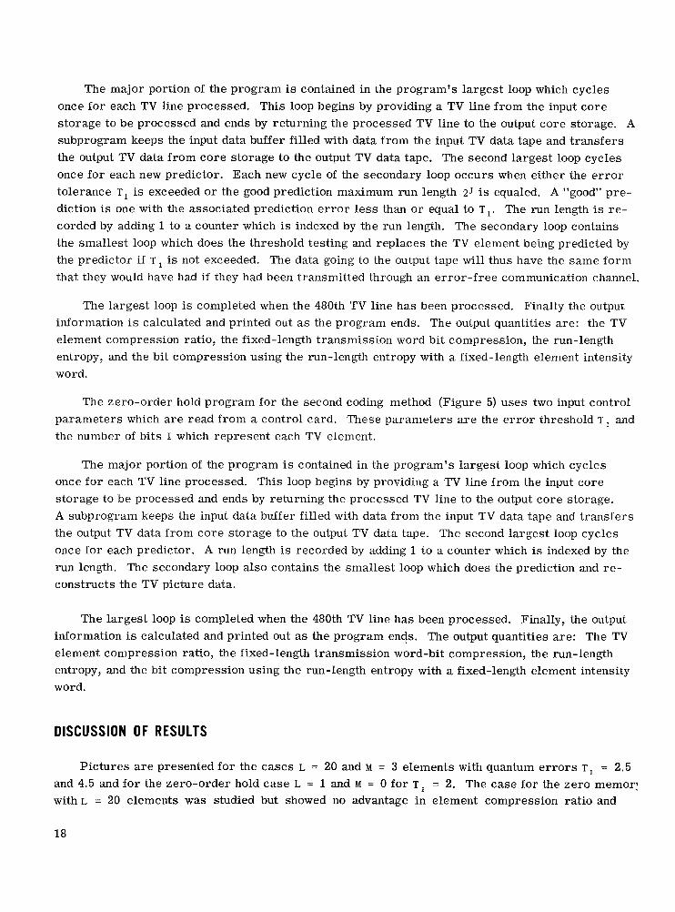
The major portion of the program is contained in the program's largest loop which cycles once for each TV line processed. This loop begins by providing a TV line from the input core storage to be processed and ends by returning the processed TV line to the output core storage. A subprogram keeps the input data buffer filled with data from the input TV data tape and transfers the output TV data from core storage to the output TV data tape. The second largest loop cycles once for each new predictor. Each new cycle of the secondary loop occurs when either the e r r o r tolerance T , is exceeded or the good prediction maximum run length 2J is equaled. A "good" prediction is one with the associated prediction e r r o r less than or equal to T I . The run length is r e - corded by adding 1 to a counter which is indexed by the run length. The secondary loop contains the smallest loop which does the threshold testing and replaces the TV element being predicted by the predictor i f T , is not exceeded. The data going to the output tape will thus have the same form that they would have had if they had been transmitted through an error-free communication channel.

The largest loop is completed when the 480th TV line has been processed. Finally the output information is calculated and printed out as the program ends. The output quantities are: the TV element compression ratio, the fixed-length transmission word bit compression, the run-length entropy, and the bit compression using the run-length entropy with a fixed-length element intensity word.

The zero-order hold program for the second coding method (Figure 5) uses two input control parameters which a r e read from a control card. These parameters a r e the e r r o r threshold T I and the number of bits I which represent each TV element.

The major portion of the program is contained in the program's largest loop which cycles once for each TV line processed. This loop begins by providing a TV line from the input core storage to be processed and ends by returning the processed TV line to the output core storage. A subprogram keeps the input data buffer filled with data from the input TV data tape and transfers the output TV data from core storage to the output TV data tape. The second largest loop cycles once for each predictor. A run length is recorded by adding 1 to a counter which is indexed by the run length. The secondary loop also contains the smallest loop which does the prediction and r e - constructs the TV picture data.

The largest loop is completed when the 480th TV line has been processed. Finally, the output information is calculated and printed out as the program ends. The output quantities are: The TV element compression ratio, the fixed-length transmission word-bit compression, the run-length entropy, and the bit compression using the run-length entropy with a fixed-length element intensity word.

DISCUSSION OF RESULTS

Pictures a r e presented for the cases L = 20 and M = 3 elements with quantum e r r o r s T , = 2.5 and 4.5 and for the zero-order hold case L = 1 and M = 0 for T , = 2. The case for the zero memor! with^ = 20 elements was studied but showed no advantage in element compression ratio and

18

thus no pictures were prepared for it. The element compression ratio is considered the most meaningful value in separating the question of optimum coding from the prediction problem.

7(c)

4.14

2.36

Element and bit compression ratios for Figures 6(c) to 15(c) with L = 20, M = 3, K = 0, T, = 2.5, and T, = 3.0 a r e given in Table 1. Figures 6(c) to 9(c) show essentially the same cloud features; the element compression ratios vary from 4.14 to 3.43 with an average ratio of approximately 3.8. It can be seen from a comparison of the digital originals with the compressed copies of these figures that the compressed pictures have areas with long horizontal stretches of equal brightness although the digital originals show random changes in these same areas. That this is a consequence of the chosen e r r o r limit as well as of the prediction technique is evident since the zero-order hold case with e r ro r limits the same as those used with the L = 20, M = 3, case gives poorer picture quality. Pictures prepared by the zero-order hold technique clearly illustrate this degradation, although many important structural details a r e preserved. For instance, Figure 4 shows a large gray a rea of broken cumulus clouds and a thin haze of, possibly, c i r rus clouds; a small bright cloud spot can be located by measuring 3/4 of the length of the fiducial mark from the corner of the lower left fiducial mark and drawing lines parallel to the mark. This cloud apparently projects higher than its surrounding cumuli because it is illuminated brighter than its surroundings; the same spot can be located in the digital original and the processed picture. When the satellite movement is followed on the picture sequence this cloud feature can be located with difficulty on the original analog Figures 6(a) to 9(a). It is much less clear on the digital originals, except in Figure 7(b), and also less clear on the processed pictures. Other details like the bright streaks running parallel to the field in the centrally located cloud field of Figure 8 a re less pronounced in the digital originals but appear with identical definition on the processed pictures (Figures 6(c) to 9(c)).

The appearance of Figures 10 and 11 is entirely different and the pictures show no distinct patterns. Element compression ratios of 3.51 and 3.19 were achieved for Figures lO(c) and l l ( c ) and an average compression ratio close to the average for the preceding four frames was obtained. Few distinct features can be located except for the tearing of apparently high-rising cumulus clouds because of convection. In Figure 10 there is an elliptically shaped cloud with a darker center spot in the lower left quadrant, located by drawing lines parallel to the mark, one bisecting the horizontal mark and the other intersecting the vertical portion 3/4 of the way up the lower left fiducial

8(c) 9(c) 1O(c)

3.43 4.09 3.51

2.04 2.30 2.04

Table 1

El em ent 1. F i g u i e T

Element compression rat io

k p r ess ion rat io

*Average number

3.79

2.15

of bits

- Av.*

3.56

2.09

~

19

mark. The longer dimension of this spot seems to be about 10 TV lines wide. It can be seen with equal clarity in both originals and in the processed picture. In the clear-to-hazy area in the lower right-hand section there are broken elongated sections where the very dark ocean is visible under- neath. These sections appear equally well on all copies. An apparently high cirrus field at the center right can be surmised as such in the analog original but is difficult to recognize in the digital original. The processed picture shows the same quality as the digital original.

The next picture(Figure 12) is taken from Tiros V over the general vicinity of Bermuda and shows a distinct cloud grouping with arclike patterns in the right half of it. The fine structure and horizontal variation in the lower left third of the picture a r e due to bad detection of the synchroni- zation pulse caused presumably by poor S/N ratio in the receiver. Although no record of the received field strength is available it is reasonable to assume that Tiros was low at the horizon as seen from the Wallops Island receiving site. The quality of the processed picture (Figure 12(c)) is as good as that of the previous processed pictures and the compression ratio of 3.45 is reasonable.

Figure 13 shows a decaying hurricane or cyclone off Miami and has the poorest element compression ratio. Comparison of the analog and digital originals shows a marked increase in gray background noise, presumably because of bad adjustment of the video amplifier ahead of the A/D converter. The effect of this higher level of background noise is the poorest element compression ratio produced for any of the pictures. This is much in contrast with what one expects by comparison with the preceding three pictures. The much higher element compression ratio of Figure 15(c) which shows a similar pattern and a considerably extended sky a rea also points to this conclusion.

Comparison of the analog and digital originals of Figure 14 shows a loss in definition of the possible storm center in the upper left third section of the photograph near the horizon. The sus- picion of a storm center is partly suggested from knowledge of the succeeding frame delivered which is not included in this series. The processed picture shows no loss other than in the digital original and has approximately the same element compression ratio as do the previous pictures. The final picture is of a classic cyclone located northeast of Bermuda in May 1963. The pronounced pattern and the large sky portion offer the suggestion that better prediction should be achieved than in any of the other pictures, particularly better than in Figures 10 and 11. Comparison of the originals and the processed copy reveals no significant loss in detail even though the compression ratio was the highest of all.

For comparison the analysis was repeated using five-bit data and permitting a quantum e r r o r of 54.5 quantum steps. The element and bit compression ratios given in Table 2 were achieved with L = 20, M = 3; K = 0, T , = 4.5, and T, = 5.0. It should be noted that with such a large e r r o r tolerance (9 out of 32 possible levels) only a coarse intensity gradation is achieved. While any one of the 32 possible amplitudes can affect the reproduced picture, dividing the total range by the nine quantum e r ro r levels yields only three and a half center levels which significantly degrade the gray scale of the original picture. The most disturbing feature of this picture ser ies is the constant amplitude over extended line segments. This streakiness is a direct consequence of the coarse e r r o r tolerance. Large quantum e r r o r s can thus be eliminated from further consideration.

Figures 6(e) to 15(e) were produced with T , = 2 for L = 1 and M = 0, the zero-order hold case, and with the following compression and bit ratios given in Table 3. As can be seen by comparison

20

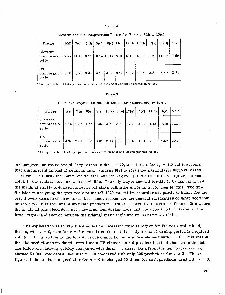
Table 2

Element and Bit Compression Ratios for Figures 6(d) to 15(d).

12(e)

4.43

2.48

Figure

Element compress ion rat io

Bit compression ratio

13(e) 14(e)

2.29 4.15

1.54 2.39

3.80

7(d)

11.10

5.26

8(d)

6.92

3.42

10.34 10.17

4.98 4.86

11.90

5.50

*Average number of bits per picture converted to element and bit compression ratios.

Table 3

Element Compression and Bit Ratios for Figure.s 6(e) to 15(e).

Figure

Element compression rat io

Bit compression rat io

6(e)

5.42

2.94

7(e)

4.88

2.64

8(e)

4.55

2.51

4.93 3.71

2.67 2.16 4.67

Av.* __

7.59

3.84

-

Av.* -

4.22

2.43

*Average number of bits per picture converted to element and bit compression ratios.

the compression ratios a r e all larger than in the L = 20, M = 3 case for T , = 2.5 but i t appears that a significant amount of detail is lost. Figures 6(e) to 9(e) show particularly serious losses. The bright spot near the lower left fiducial mark in Figure 7(e) is difficult to recognize and much detail in the central cloud area is not visible. The only way to account for this is by assuming that the signal is rarely predicted correctly but stays within the e r r o r limit for long lengths. The dif- ficulties in assigning the gray scale to the SC-4020 microfilm recorder a r e partly to blame for the bright overexposure of large a reas but cannot account for the general streakiness of large sections; this is a result of the lack of accurate prediction. This is especially apparent in Figure lO(e) where the small elliptic cloud does not show a central darker a rea and the deep black patterns at the lower right-hand section between the fiducial mark angle and cross are not visible.

The explanation as to why the element compression ratio is higher for the zero-order hold, that is, with M = 0, than for M = 3 comes from the fact that only a short learning period is required with M = 0. In particular the learning period used herein was one element with M = 0. This means that the predictor is up-dated every time a TV element is not predicted so that changes in the data are followed relatively quickly compared with the M = 3 case. Data from the ten picture average showed 53,000 predictors used with M = 0 compared with only 800 predictors for M = 3. figures indicate that the predictor for M = 0 is changed 66 times for each predictor used with M = 3.

These

21

I .

The economy of learning with M = 0 allows frequent up-dating of the predictor so that even though the zero-order hold neither predicts as well nor maintains its quality for as long as the M = 3 case a higher compression ratio is still achieved with it. A second method also given by Bala- krishnan and referred to as Method I1 in Reference 1 has been programed and has yielded results with better element compression ratios than has the zero-order hold.

CONCLUSIONS

Compression ratios achieved offer sufficient promise to continue the investigation and refine the method. A comparison of the results obtained using M = 0 with those obtained using M = 3 suggests that the two cases be combined and the constant term in the M = 3 case be replaced by the zero-order hold. The learning e r ro r may be more conveniently controlled and a better solution therefore found if the steepest descents solution is used in solving for the weights as mentioned in Reference 1. At the time of this writing preliminary results a r e available using Method II of Reference 1 which show even better compression ratios than those reported herein. optimization of the parameters chosen remains to be accomplished and the corresponding effect on picture quality determined.

Further

ACKNOWLEDGMENTS

The authors a r e indebted to Herbert J. Gillus who programed the IBM 7094 and to Joseph A. Sciulli who obtained the ten TV pictures and checked the manuscript.

(Manuscript received August 3 1 , 1965)

REFERENCES

1. Balakrishnan, A. B., "An Adaptive Non-Linear Data Predictor," Paper No. 6-5, Proc. 1962 National Telemetering Conf. (May 23-25, 1962, Washington, D. C.), The Institute of Radio Engineers, New York N.Y., 1962.

2. Hestenes, M. R., and Stiefel, E., "Method of Conjugate Gradients for Solving Linear Equations," J. Res. Nat. Bur. Standards 49(6):409-436, December 1952.

22

. "t

(b) Digital original.

-.a e

(c) Linear predictor with 2 quantum steps error. Processed copy; t i = 2.5; t 2 = 3.0; L = 20; M 3; K = 0; element compression, 3 79; bit compresslon for fixed-length code of 6 bits per data word,

2 15.

Figure 6-Pictures from Tiros I l l , orbit 4, frame 2, camera 2, direct transmission from sate I I i te.

, , (e) Zero order hold with 2 quantum steps error.

Processed copy; t i = 2 0; L = 1; M = 0; element compression, 5.42; bit compression for fixed-length code of 6 bi ts per dota word, 2.94 23

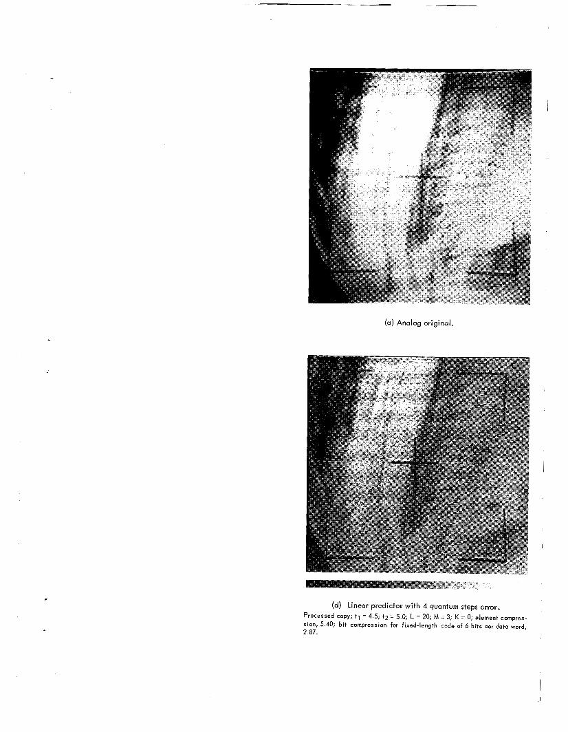
(a) Analog original.

(d) Linear predictor with 4 quantum steps error. Processed copy; t l = 4.5 t 2 = 5.0; L = 20; M = 3; K = 0; element compression, 7.29; bit compression for fixed-length code o f 6 bits per data word, 3.80.

I (b) Digital original. (c) Linear predictor with 2 quantum steps error. Processed copy; t i = 2.5; t i 3.0; L = 20; M = 3; K = 0; element compression, 4.14; b i t compression for fixed-length code of 6 bits per data word,

2.36.

Figure 7-Pictures from Tiros Ill, orbit 4, frame 3; camera 2; direct transmission from satellite.

(e) Zero order hold with 2 quantum steps error.

Processed copy; t i = 2.0; L = 1; M = 0; element compression, 4.88; bi t compression for fixed-length code of 6 bits per data word, 2.64.

25


(4 Linear predictor with 4 quantum steps error. Processed copy; t i = 4 5; tq 5 0, L = 20; M = 3, K = 0; element compression, 11.10, bit compresslon for fixed-length code o f 6 bits per doto word, 5.26.


(e) Zero order hold with 2 quantum steps error. Processed copy; t i 2.0; L 1; M = 0; element compression, 4.55; bit compression for fixed-length code of 6 bits per data word, 2 .51.

(c) Linear predictor with 2 quantum steps error. Processed copy; t i = 2.5; t2 = 3.0; L z 20; M = 3; K = 0; element compression, 3.43; bit compression for fixed-length code o f 6 bits per data word, 2.04.

Figure 8-Pictures from Tiros 1 1 1 , orbit 4, frame 4, camera 2, direct transmission from satellite.

27

(a) Analog original. ~ ,

(d) Linear predictor with 4 quantum steps error. Processed copy; t l 4.5; t2 = 5.0; L = 20; M = 3; K = 0; element compression, 6.92; bit compression for fixed-length code of 6 bits per data word, 3.42.

i % *

(b) Digital original. (c) Linear predictor with 2 quantum steps error. Processed copy; t l = 2.5; t 2 3.0; L = 20; M = 3; K = 0; element compression, 4.09; bit compression for fixed-length code of 6 b i ts per data word, 2.30.

Figure 9-Pictures from Tiros Ill, orbit 4, frame 5, camera 2, direct transmission from satellite.

(e) Zero order hold with2quantum steps error. Processed copy; t l = 2.0; L = 1; M = 0; element compression, 4.93; bit compression for fixed-length code of 6 b i ts per data word, 2.67.

29

(a) Analog original. I

(d) Linear predictor with 4 quantum steps error.

Processed copy, t i = 4 5; t2 = 5 0; L 20; M = 3; K 0; element compression, 10 34; bit compression for fixed-length code of 6 bits per dato word, 4 98.


(e) Zero order hold with2quantum steps error. Processed copy; t i = 2 0, L = 1, M = 0, element compresslon, 3 71, btt

compresslon for fixed-length code of 6 blts per data word, 2 16.

(c) Linear predictor with 2 quantum steps error.

Processed copy; t l = 2.5; tZ = 3.0; L = 20; M = 3; K = 0; element compression, 3.51; b i t compression for fixed-length code of 6 b i ts per data word, 2.04.

Figure 10-Pictures from Tiros Ill, orbit 102, frame 1, camera 1 , taped before transmission from satel lite.

31


*e

(d) Linear predictor with 4 quantum steps error. Processed copy; t i = 4 5; t 2 = 5.0; L = 20; M 3; K = 0; element compression, 10 17, bi t compression for fixed-length code of 6 bi ts per data word, 4 86.

I


(e) Zero order hold with2quantum steps error. - . . . . Processed copy; t , = 2.0; L = 1; M = 0; element compression, 3.60; bi t compression for fixed-length code of 6 bits per dot0 word, 2.1 1.

(c) Linear predictor with 2 quantum steps error. processed copy; t , = 2.5; t 2 = 3.0; L = 20; M = 3; K = 0; element compression, 3.19; bit compression for fixed-length code of 6 bits per doto word,

Figure 11 -pictures from Tiros I l l , orbit 102, frame 2, camera 1 , taped before transmission from sate) lite.

33


(d) Linear predictor with 4 quantum steps error. Processed COPY; t i = 4.5; t 2 = 5.0; L = 20; M = 3; K = 0; element compression, 6.18; bi t compression for fixed-length code of 6 b i ts per data word,

3.25.

,

(b) Digital original. (c) Linear predictor with 2 quantum steps error.

processed t l = 2.5; t 2 = 3.0; L = 20; M = 3; K = 0; element compression, 3.45; bit compression for fixed-length code of 6 bits per doto word.

2.08.

Figure 12-Pictures from Tiros V, orbit 3143, frame 7, camera 1 , direct transmission from satellite.

(e) Zero order hold with2quantum steps error. Processed copy; t i = 2.0; L = 1; M = 0; element compression, 4.43; bit compression for fixed-length code of 6 bits per data word, 2.48. i 35


L

(d) Linear predictor with 4 quantum steps error. - I Processed COPY; t i

sion, 5.40; bit compression for fixed-length code of 6 bits per &to word, 2.87.

4.5; t i = 5.0; L = 20; M = 3; K = 0; element ,


(e) Zero order hold with 2quontum steps error. Processed copy; t i = 2.0; L = 1 ; M = 0; element compression, 2.29; bit compression for fixed-length code of 6 bits per doto word, 1.54.

(c) Linear predictor with 2 quantum steps error. Processed copy; t i = 2.5; t z = 3.0; L = 20; M = 3; K = 0; element compres-

sion, 2.29; bit compression for fixed-length code of 6 b i ts per data word,

1.49.

Figure 13-Pictures from Tiros VI, orbit 11 00, frame 15, camera 1 , direct transmission from satellite.

37

(a) Analog original

(d) Linear predictor with 4 quantum steps error. Processed COPY; t i = 4.5; t z = 5.0; L = 30; M = 3; K 0; element compression, 5.39; bi t compression for fixed-length code o f 6 bits per data word, 2.85.


39

.


(d) Linear predictor with 4 quantum steps error. Processed copy; t I = 4.5; t2 = 5.0; L = 20; M = 3; K = 0. sion, 7.47; bit compression for fixed-length 3.81.

I element compres- of 6 ,,its per doto word,


(e) Zero order hold with2quantum steps error. Processed copy; t i = 2.0; L = 1; M = 0; element compression, 9.50; bi t compression for fixed-length code o f 6 bits per data word, 4.67.

(c) Linear predictor with 2 quantum steps error. Processed copy; t i = 2 5; t 2 = 3 0; L = 30; M = 3; K = 0; element compres slon, 6.27; bit compression for fixed-length code of 6 bi ts pet data word, 3.35.

Figure 15-Pictures from Tiros VI, orbit 3692, frame 31, camera 1 , taped before transmission from satellite.

41


b

(d) Linear predictor with 4 quantum steps error. Processed copy; t i = 4.5; t 2 5.0; L = 20; M = 3; K = 0; element compression, 11.90; bit compression for fixed-length code of 6 bits per data wwd, 5.50.

Appendix A

Symbols

B bandwidth (cps)

c symmetric positive cost function

Pr probability of exceedence of threshold

pi probability numbers

D determinant R = S T S

f frequency s memory matrix

G = S T P

I TV element intensity o r run-length bits information

J run length bits

K constant associated with each prediction

I

k number of elements in run greater than one

sT transpose of s T duration of waveform

T, preset threshold of difference between prediction and data element, the quantum e r ro r

T, periodic average prediction e r ro r threshold

t time parameter

t o value of t in interval o < t < T - n

w weight vector containing set L learning period, the number of picture

elements from which weighing function is derived; also, length x( t ) continuous o r discrete parameter

of M f 1 weights

source

M memory, the number of picture elements X* (to t A) predicted value of data preceding data point to be predicted used to make each prediction xn data samples

yn N-column vector

N number of bits per transmitted word aj optimal filter weights

n number of sample A differential of time

o prediction operator E prediction e r ro r

p ( t ) positive weight function

P column vector of TV elements u dummy variable of time

43

Documents

m OI m T COPY: (WLIL-2) n AFB, z c · FOR VIDEO SIGNALS bY ... The ten Tiros television cloud pictures used in the study ... A detailed explanation of how the technique is applied