Embed Size (px)
Citation preview
MATLAB Tutorial Course
1

Contents Continued
Desktop tools matrices Logical &Mathematical operations Handle Graphics Ordinary Differential Equations (ODE)
4
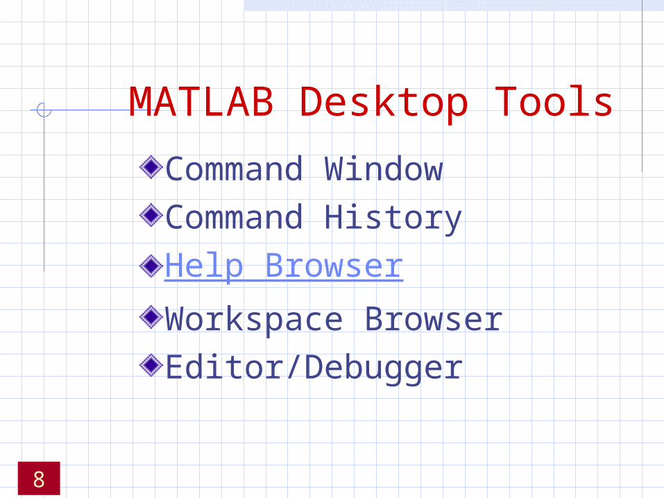
MATLAB Desktop Tools
Command WindowCommand HistoryHelp BrowserWorkspace BrowserEditor/Debugger
8
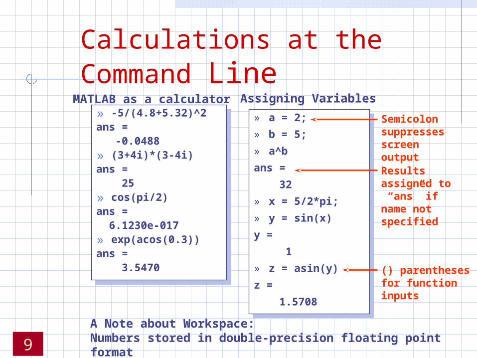
Calculations at the Command Line
» a = 2;
» b = 5;
» a^b
ans =
32
» x = 5/2*pi;
» y = sin(x)
y =
1
» z = asin(y)
z =
1.5708
» a = 2;
» b = 5;
» a^b
ans =
32
» x = 5/2*pi;
» y = sin(x)
y =
1
» z = asin(y)
z =
1.5708
Results assigned to “ans” if name not specified
() parentheses for function inputs
Semicolon suppresses screen output
MATLAB as a calculator Assigning Variables
A Note about Workspace:Numbers stored in double-precision floating point format
» -5/(4.8+5.32)^2ans = -0.0488» (3+4i)*(3-4i)ans = 25» cos(pi/2)ans = 6.1230e-017» exp(acos(0.3))ans = 3.5470
» -5/(4.8+5.32)^2ans = -0.0488» (3+4i)*(3-4i)ans = 25» cos(pi/2)ans = 6.1230e-017» exp(acos(0.3))ans = 3.5470
9

General Functions whos: List current variables clear: Clear variables and functions from memoryClose: Closes last figures cd: Change current working directory dir: List files in directory echo: Echo commands in M-files format: Set output format
10
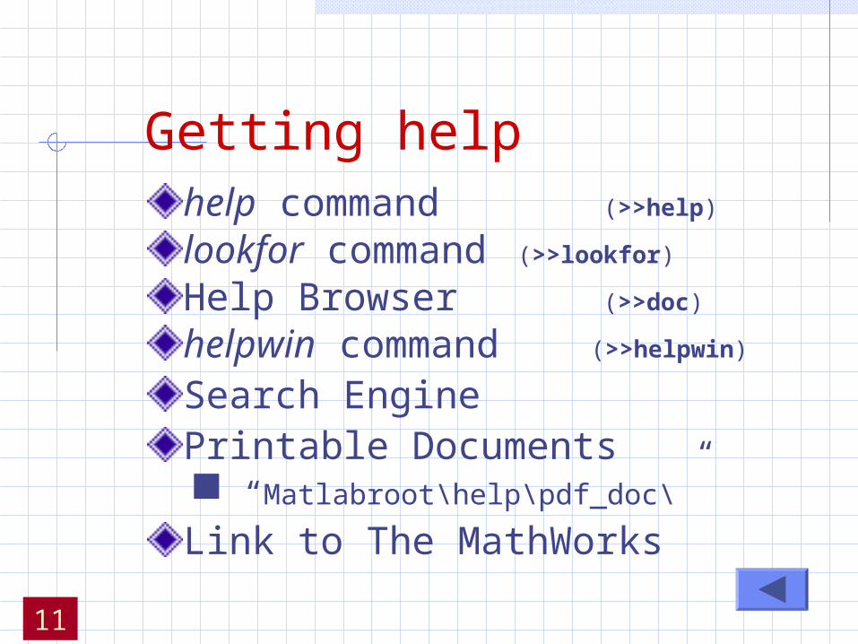
Getting helphelp command (>>help)
lookfor command (>>lookfor)
Help Browser (>>doc)
helpwin command (>>helpwin)
Search EnginePrintable Documents “Matlabroot\help\pdf_doc\”
Link to The MathWorks
11

MatricesEntering and Generating MatricesConcatenationDeleting Rows and ColumnsArray ExtractionMatrix and Array Multiplication
12

» a=[1 2;3 4]
a =
1 2
3 4
» b=[-2.8, sqrt(-7), (3+5+6)*3/4]
b =
-2.8000 0 + 2.6458i 10.5000
» b(2,5) = 23
b =
-2.8000 0 + 2.6458i 10.5000 0 0
0 0 0 0 23.0000
» a=[1 2;3 4]
a =
1 2
3 4
» b=[-2.8, sqrt(-7), (3+5+6)*3/4]
b =
-2.8000 0 + 2.6458i 10.5000
» b(2,5) = 23
b =
-2.8000 0 + 2.6458i 10.5000 0 0
0 0 0 0 23.0000
•Any MATLAB expression can be entered as a matrix element
•Matrices must be rectangular. (Set undefined elements to zero)
Entering Numeric Arrays
Row separatorsemicolon (;)
Column separatorspace / comma (,)
Use square brackets [ ]
13

The Matrix in MATLAB
4 10 1 6 2
8 1.2 9 4 25
7.2 5 7 1 11
0 0.5 4 5 56
23 83 13 0 10
1
2
Rows (m) 3
4
5
Columns(n)
1 2 3 4 51 6 11 16 21
2 7 12 17 22
3 8 13 18 23
4 9 14 19 24
5 10 15 20 25
A = A (2,4)
A (17)
Rectangular Matrix:Scalar: 1-by-1 arrayVector: m-by-1 array
1-by-n arrayMatrix: m-by-n array14
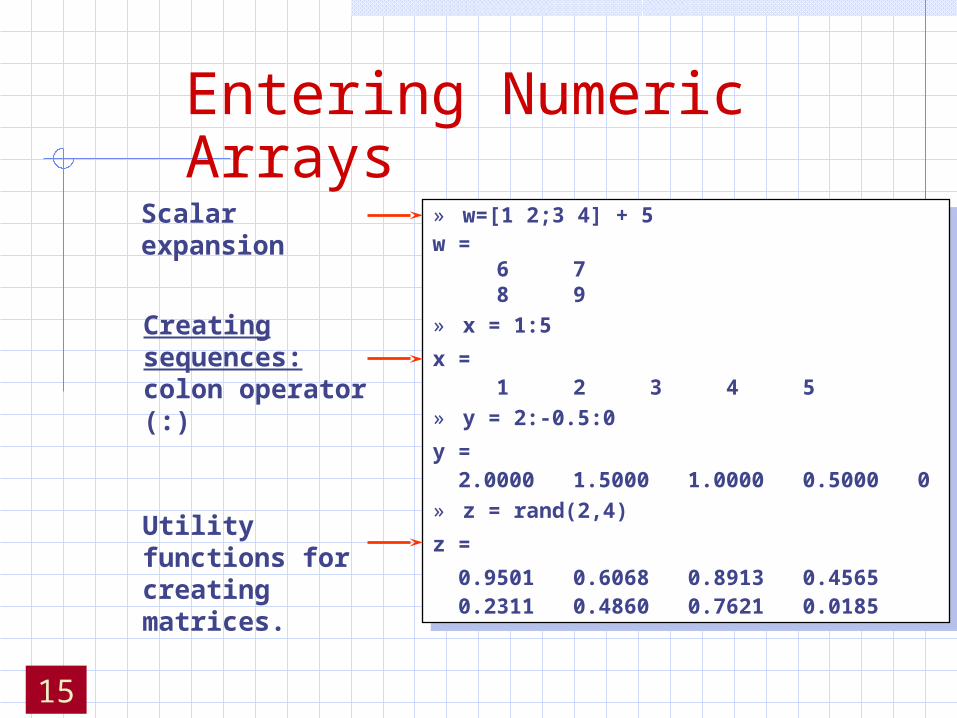
» w=[1 2;3 4] + 5w = 6 7 8 9» x = 1:5
x = 1 2 3 4 5» y = 2:-0.5:0
y = 2.0000 1.5000 1.0000 0.5000 0 » z = rand(2,4)
z =
0.9501 0.6068 0.8913 0.4565 0.2311 0.4860 0.7621 0.0185
» w=[1 2;3 4] + 5w = 6 7 8 9» x = 1:5
x = 1 2 3 4 5» y = 2:-0.5:0
y = 2.0000 1.5000 1.0000 0.5000 0 » z = rand(2,4)
z =
0.9501 0.6068 0.8913 0.4565 0.2311 0.4860 0.7621 0.0185
Scalar expansion
Creating sequences:colon operator (:)
Utility functions for creating matrices.
Entering Numeric Arrays
15
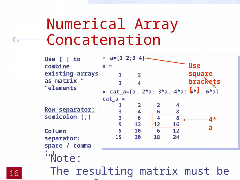
Numerical Array Concatenation
» a=[1 2;3 4]
a =
1 2
3 4
» cat_a=[a, 2*a; 3*a, 4*a; 5*a, 6*a]cat_a = 1 2 2 4 3 4 6 8 3 6 4 8 9 12 12 16 5 10 6 12 15 20 18 24
» a=[1 2;3 4]
a =
1 2
3 4
» cat_a=[a, 2*a; 3*a, 4*a; 5*a, 6*a]cat_a = 1 2 2 4 3 4 6 8 3 6 4 8 9 12 12 16 5 10 6 12 15 20 18 24
Use [ ] to combine existing arrays as matrix “elements”
Row separator:semicolon (;)
Column separator:space / comma (,)
Use square brackets [ ]
Note:The resulting matrix must be rectangular
4*a
16

Deleting Rows and Columns
» A=[1 5 9;4 3 2.5; 0.1 10 3i+1]
A =
1.0000 5.0000 9.0000
4.0000 3.0000 2.5000
0.1000 10.0000 1.0000+3.0000i
» A(:,2)=[]
A =
1.0000 9.0000
4.0000 2.5000
0.1000 1.0000 + 3.0000i
» A(2,2)=[]
??? Indexed empty matrix assignment is not allowed.
» A=[1 5 9;4 3 2.5; 0.1 10 3i+1]
A =
1.0000 5.0000 9.0000
4.0000 3.0000 2.5000
0.1000 10.0000 1.0000+3.0000i
» A(:,2)=[]
A =
1.0000 9.0000
4.0000 2.5000
0.1000 1.0000 + 3.0000i
» A(2,2)=[]
??? Indexed empty matrix assignment is not allowed.
17
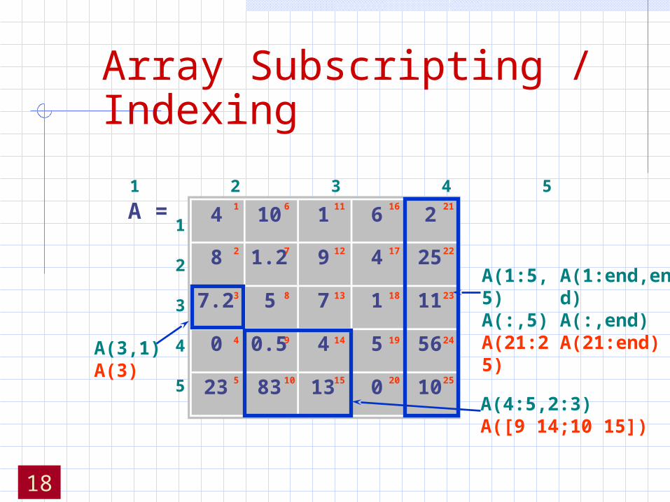
Array Subscripting / Indexing
4 10 1 6 2
8 1.2 9 4 25
7.2 5 7 1 11
0 0.5 4 5 56
23 83 13 0 10
1
2
3
4
5
1 2 3 4 51 6 11 16 21
2 7 12 17 22
3 8 13 18 23
4 9 14 19 24
5 10 15 20 25
A =
A(3,1)A(3)
A(1:5,5)A(:,5) A(21:25)
A(4:5,2:3)A([9 14;10 15])
A(1:end,end) A(:,end)A(21:end)’
18

Matrix Multiplication» a = [1 2 3 4; 5 6 7 8];
» b = ones(4,3);
» c = a*b
c =
10 10 10 26 26 26
» a = [1 2 3 4; 5 6 7 8];
» b = ones(4,3);
» c = a*b
c =
10 10 10 26 26 26
[2x4]
[4x3]
[2x4]*[4x3] [2x3]
a(2nd row).b(3rd column)
» a = [1 2 3 4; 5 6 7 8];
» b = [1:4; 1:4];
» c = a.*b
c =
1 4 9 16 5 12 21 32
» a = [1 2 3 4; 5 6 7 8];
» b = [1:4; 1:4];
» c = a.*b
c =
1 4 9 16 5 12 21 32 c(2,4) = a(2,4)*b(2,4)
Array Multiplication
19
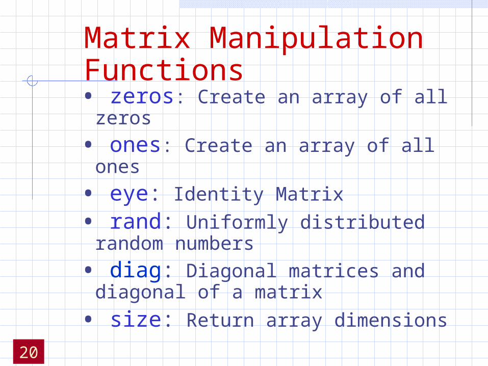
Matrix Manipulation Functions• zeros: Create an array of all zeros
• ones: Create an array of all ones
• eye: Identity Matrix
• rand: Uniformly distributed random numbers
• diag: Diagonal matrices and diagonal of a matrix
• size: Return array dimensions
20

Matrix Manipulation Functions• transpose (’): Transpose matrix • rot90: rotate matrix 90
• tril: Lower triangular part of a matrix
• triu: Upper triangular part of a matrix
• cross: Vector cross product
• dot: Vector dot product
• det: Matrix determinant
• inv: Matrix inverse
• eig: Evaluate eigenvalues and eigenvectors• rank: Rank of matrix
21
Elementary MathLogical Operators
Math Functions
25

Logical Operations
» Mass = [-2 10 NaN 30 -11 Inf 31];» each_pos = Mass>=0each_pos = 0 1 0 1 0 1 1» all_pos = all(Mass>=0)all_pos = 0» all_pos = any(Mass>=0)all_pos = 1» pos_fin = (Mass>=0)&(isfinite(Mass))pos_fin = 0 1 0 1 0 0 1
» Mass = [-2 10 NaN 30 -11 Inf 31];» each_pos = Mass>=0each_pos = 0 1 0 1 0 1 1» all_pos = all(Mass>=0)all_pos = 0» all_pos = any(Mass>=0)all_pos = 1» pos_fin = (Mass>=0)&(isfinite(Mass))pos_fin = 0 1 0 1 0 0 1
= = equal to
> greater than
< less than
>= Greater or equal
<= less or equal
~ not
& and
| or
isfinite(), etc. . . .
all(), any()
find
Note:• 1 = TRUE• 0 = FALSE
26

Elementary Math Function• abs, sign: Absolute value and Signum
Function• sin, cos, asin, acos…: Triangular functions• exp, log, log10: Exponential, Natural and
Common (base 10) logarithm• ceil, floor: Round toward infinities• fix: Round toward zero
27

Elementary Math Function
round: Round to the nearest integer gcd: Greatest common devisor lcm: Least common multiple sqrt: Square root function real, imag: Real and Image part of complex rem: Remainder after division

Elementary Math Function
• max, min: Maximum and Minimum of arrays• mean, median: Average and Median of arrays • std, var: Standard deviation and variance • sort: Sort elements in ascending order• sum, prod: Summation & Product of Elements
28
Graphics Fundamentals
35
GraphicsBasic Plotting
plot, title, xlabel, grid, legend, hold, axis
Editing Plots Property Editor
36

2-D Plotting
Syntax:
Example:
plot(x1, y1, 'clm1', x2, y2, 'clm2', ...)plot(x1, y1, 'clm1', x2, y2, 'clm2', ...)
x=[0:0.1:2*pi];y=sin(x);z=cos(x);plot(x,y,x,z,'fontsize',14);legend('Y data','Z data ,'linewidth',2)title('Sample Plot','fontsize',14);xlabel('X values','fontsize',14);ylabel('Y values', data')grid on
x=[0:0.1:2*pi];y=sin(x);z=cos(x);plot(x,y,x,z,'fontsize',14);legend('Y data','Z data ,'linewidth',2)title('Sample Plot','fontsize',14);xlabel('X values','fontsize',14);ylabel('Y values', data')grid on
37

Sample Plot
Title
Ylabel
Xlabel
Grid
Legend
38
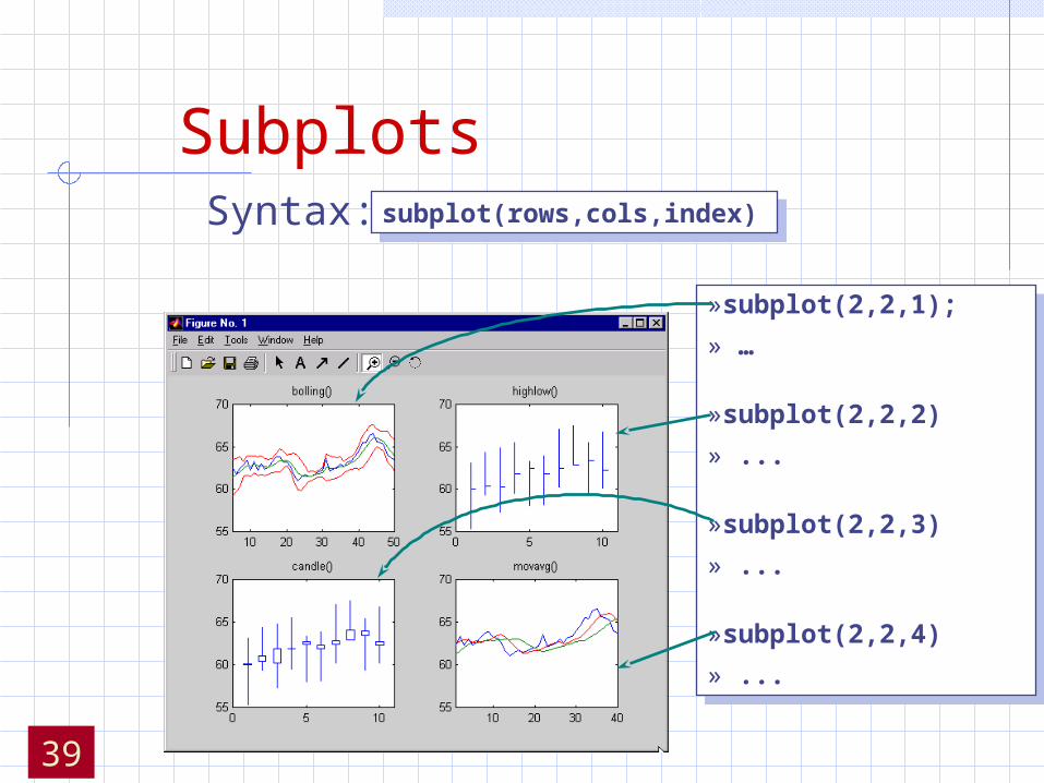
SubplotsSyntax:
»subplot(2,2,1);
» …
»subplot(2,2,2)
» ...
»subplot(2,2,3)
» ...
»subplot(2,2,4)
» ...
»subplot(2,2,1);
» …
»subplot(2,2,2)
» ...
»subplot(2,2,3)
» ...
»subplot(2,2,4)
» ...
subplot(rows,cols,index)subplot(rows,cols,index)
39

Programming andApplication Development
45
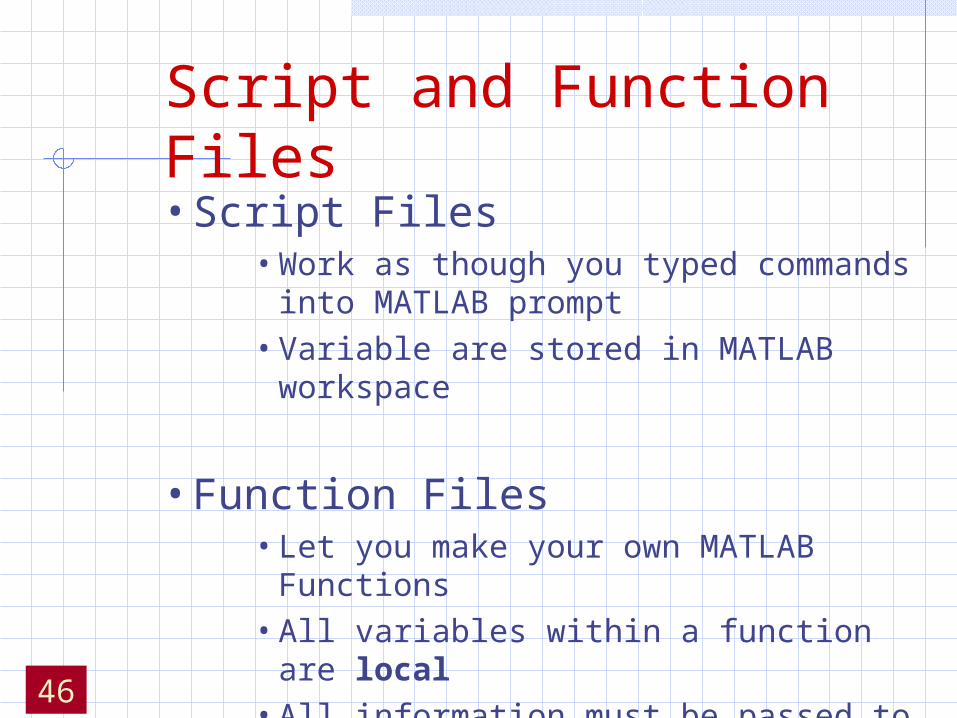
Script and Function Files
• Script Files• Work as though you typed commands into
MATLAB prompt
• Variable are stored in MATLAB workspace
• Function Files• Let you make your own MATLAB Functions
• All variables within a function are local
• All information must be passed to functions as parameters
• Subfunctions are supported46

Basic Parts of a Function M-File
function y = mean (x)
% MEAN Average or mean value.
% For vectors, MEAN(x) returns the mean value.
% For matrices, MEAN(x) is a row vector
% containing the mean value of each column.
[m,n] = size(x);
if m == 1
m = n;
end
y = sum(x)/m;
Output Arguments Input ArgumentsFunction Name
Online Help
Function Code
47

if ((attendance >= 0.90) & (grade_average >= 60))
pass = 1;
end;
if ((attendance >= 0.90) & (grade_average >= 60))
pass = 1;
end;
eps = 1;
while (1+eps) > 1
eps = eps/2;
end
eps = eps*2
eps = 1;
while (1+eps) > 1
eps = eps/2;
end
eps = eps*2
if Statement
while Loops
Flow Control Statements
48
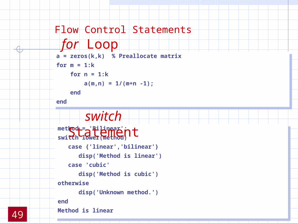
a = zeros(k,k) % Preallocate matrix
for m = 1:k
for n = 1:k
a(m,n) = 1/(m+n -1);
end
end
a = zeros(k,k) % Preallocate matrix
for m = 1:k
for n = 1:k
a(m,n) = 1/(m+n -1);
end
end
method = 'Bilinear';
switch lower(method)
case {'linear','bilinear'}
disp('Method is linear')
case 'cubic'
disp('Method is cubic')
otherwise
disp('Unknown method.')
end
Method is linear
method = 'Bilinear';
switch lower(method)
case {'linear','bilinear'}
disp('Method is linear')
case 'cubic'
disp('Method is cubic')
otherwise
disp('Unknown method.')
end
Method is linear
for Loop
switch Statement
Flow Control Statements
49

Function M-file
function r = ourrank(X,tol)
% rank of a matrix
s = svd(X);
if (nargin == 1)
tol = max(size(X)) * s(1)* eps;
end
r = sum(s > tol);
function r = ourrank(X,tol)
% rank of a matrix
s = svd(X);
if (nargin == 1)
tol = max(size(X)) * s(1)* eps;
end
r = sum(s > tol);
function [mean,stdev] = ourstat(x)[m,n] = size(x);if m == 1
m = n;endmean = sum(x)/m;stdev = sqrt(sum(x.^2)/m – mean.^2);
function [mean,stdev] = ourstat(x)[m,n] = size(x);if m == 1
m = n;endmean = sum(x)/m;stdev = sqrt(sum(x.^2)/m – mean.^2);
Multiple Input Argumentsuse ( )
Multiple Output Arguments, use [ ]
»r=ourrank(rand(5),.1);
»[m std]=ourstat(1:9);
51
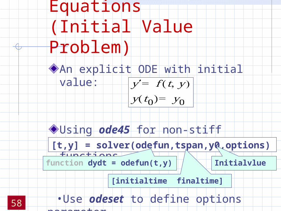
Ordinary Differential Equations(Initial Value Problem)
An explicit ODE with initial value:
Using ode45 for non-stiff functions and ode23t for stiff functions.
[t,y] = solver(odefun,tspan,y0,options)
[initialtime finaltime]
Initialvluefunction dydt = odefun(t,y)
•Use odeset to define options parameter58

ODE Example:
» [t,y]=ode45('myfunc',[0 20],[2;0])» [t,y]=ode45('myfunc',[0 20],[2;0])
function dydt=myfunc(t,y)dydt=zeros(2,1);dydt(1)=y(2);dydt(2)=(1-y(1)^2)*y(2)-y(1);
0 2 4 6 8 10 12 14 16 18 20-3
-2
-1
0
1
2
3
Note:Help on odeset to set options for more accuracy and other useful utilities like drawing results during solving.
59

??
70