Embed Size (px)
Citation preview

MMACROECONOMICSACROECONOMICS
C H A P T E R
Economic Growth II:Technology, Empirics, and Policy
8

CHAPTER 8 Economic Growth II slide 2
Introduction
In the Solow model of Chapter 7, the production technology is held constant. income per capita is constant in the steady state.
Neither point is true in the real world: 1904-2004: U.S. real GDP per person grew by a
factor of 7.6, or 2% per year. examples of technological progress abound
(see next slide).

CHAPTER 8 Economic Growth II slide 3
Technological progress in the Solow model
A new variable: E = labor efficiency
Assume: Technological progress is labor-augmenting: it increases labor efficiency at the exogenous rate g:
Eg
E
CHAPTER 8 Economic Growth II slide 4
Technological progress in the Solow model
We now write the production function as:
where L E = the number of effective workers. Increases in labor efficiency have the
same effect on output as increases in the labor force.
( , )Y F K L E
CHAPTER 8 Economic Growth II slide 5
Technological progress in the Solow model
Notation:
y = Y/LE = output per effective worker
k = K/LE = capital per effective worker
Production function per effective worker:y = f(k)
Saving and investment per effective worker:s y = s f(k)
CHAPTER 8 Economic Growth II slide 6
Technological progress in the Solow model
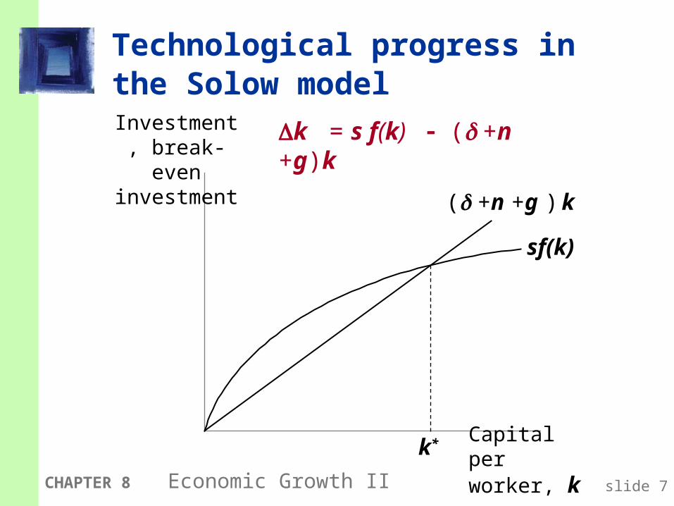
( + n + g)k = break-even investment: the amount of investment necessary to keep k constant.
Consists of: k to replace depreciating capital
n k to provide capital for new workers
g k to provide capital for the new “effective” workers created by technological progress
CHAPTER 8 Economic Growth II slide 7
Technological progress in the Solow model
Investment, break-even investment
Capital per worker, k
sf(k)
( +n +g ) k
k*
k = s f(k) ( +n +g)k
CHAPTER 8 Economic Growth II slide 8
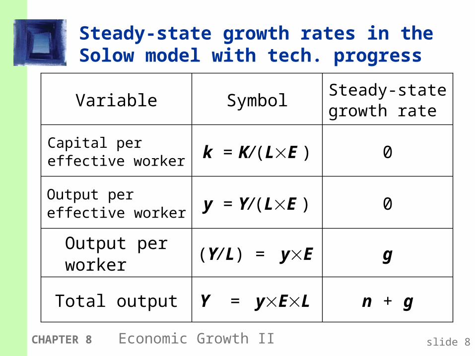
Steady-state growth rates in the Solow model with tech. progress
n + gY = yEL Total output
g(Y/ L) = yE Output per worker
0y = Y/(LE )Output per effective worker
0k = K/(LE )Capital per effective worker
Steady-state growth rate
SymbolVariable
CHAPTER 8 Economic Growth II slide 9
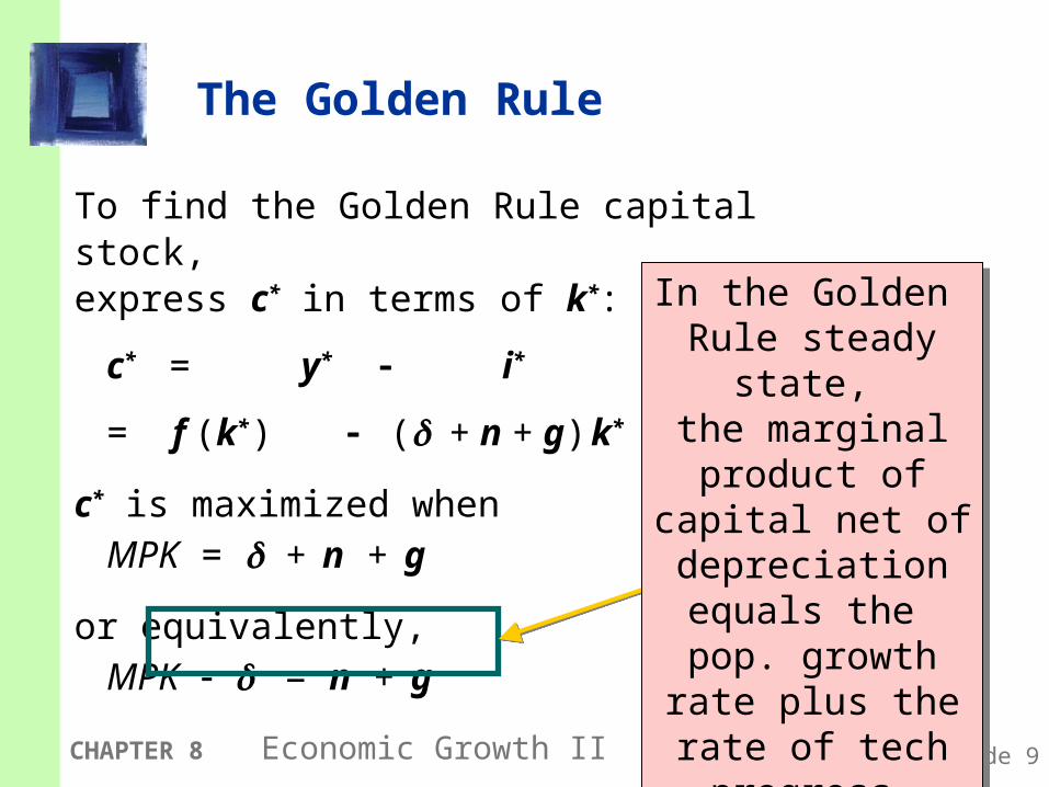
The Golden Rule
To find the Golden Rule capital stock, express c* in terms of k*:
c* = y* i*
= f (k* ) ( + n + g) k*
c* is maximized when MPK = + n + g
or equivalently, MPK = n + g
In the Golden Rule steady state,
the marginal product of capital
net of depreciation equals the
pop. growth rate plus the rate of tech progress.
In the Golden Rule steady state,
the marginal product of capital
net of depreciation equals the
pop. growth rate plus the rate of tech progress.

CHAPTER 8 Economic Growth II slide 10
Growth empirics: Balanced growth
Solow model’s steady state exhibits balanced growth - many variables grow at the same rate.
Solow model predicts Y/L and K/L grow at the same rate (g), so K/Y should be constant.
This is true in the real world.
Solow model predicts real wage grows at same rate as Y/L, while real rental price is constant.
This is also true in the real world.

CHAPTER 8 Economic Growth II slide 11
Growth empirics: Convergence
Solow model predicts that, other things equal, “poor” countries (with lower Y/L and K/L) should grow faster than “rich” ones.
If true, then the income gap between rich & poor countries would shrink over time, causing living standards to “converge.”
In real world, many poor countries do NOT grow faster than rich ones. Does this mean the Solow model fails?
CHAPTER 8 Economic Growth II slide 12
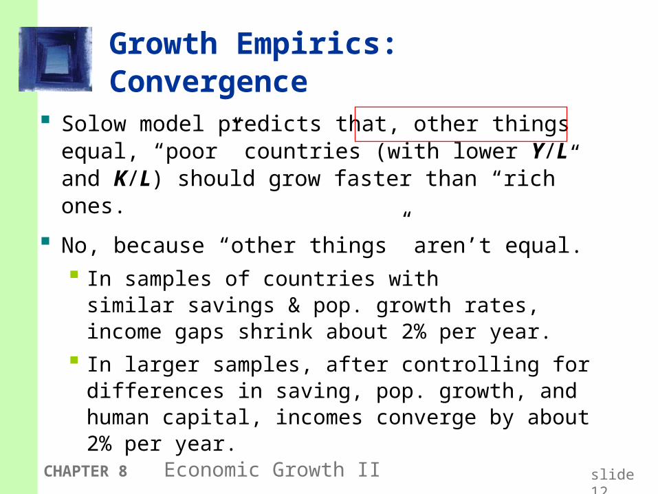
Growth Empirics: Convergence
Solow model predicts that, other things equal, “poor” countries (with lower Y/L and K/L) should grow faster than “rich” ones.
No, because “other things” aren’t equal.
In samples of countries with similar savings & pop. growth rates, income gaps shrink about 2% per year.
In larger samples, after controlling for differences in saving, pop. growth, and human capital, incomes converge by about 2% per year.
CHAPTER 8 Economic Growth II slide 13
Growth empirics: Convergence
What the Solow model really predicts is conditional convergence - countries converge to their own steady states, which are determined by saving, population growth, and education.
This prediction comes true in the real world.
CHAPTER 8 Economic Growth II slide 14
Growth empirics: Factor accumulation vs. production efficiency
Differences in income per capita among countries can be due to differences in
1. capital – physical or human – per worker
2. the efficiency of production (the height of the production function)
Studies: both factors are important. the two factors are correlated: countries with
higher physical or human capital per worker also tend to have higher production efficiency.
CHAPTER 8 Economic Growth II slide 15
Growth empirics: Factor accumulation vs. production efficiency
Possible explanations for the correlation between capital per worker and production efficiency:
Production efficiency encourages capital accumulation.
Capital accumulation has externalities that raise efficiency.
A third, unknown variable causes capital accumulation and efficiency to be higher in some countries than others.
CHAPTER 8 Economic Growth II slide 16
Policy issues: Evaluating the rate of saving
To estimate (MPK ), use three facts about the U.S. economy:
1. k = 2.5 yThe capital stock is about 2.5 times one year’s GDP.
2. k = 0.1 yAbout 10% of GDP is used to replace depreciating capital.
3. MPK k = 0.3 yCapital income is about 30% of GDP.

CHAPTER 8 Economic Growth II slide 17
Policy issues: Evaluating the rate of saving
1. k = 2.5 y
2. k = 0.1 y
3. MPK k = 0.3 y
0.1
2.5
k yk y
0.1
0.042.5
To determine , divide 2 by 1:
CHAPTER 8 Economic Growth II slide 18
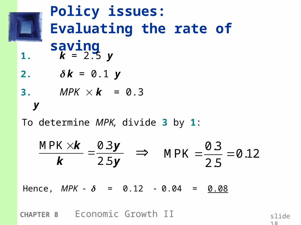
Policy issues: Evaluating the rate of saving
MPK 0.3
2.5
k yk y
0.3
MPK 0.122.5
To determine MPK, divide 3 by 1:
Hence, MPK = 0.12 0.04 = 0.08
1. k = 2.5 y
2. k = 0.1 y
3. MPK k = 0.3 y
CHAPTER 8 Economic Growth II slide 19
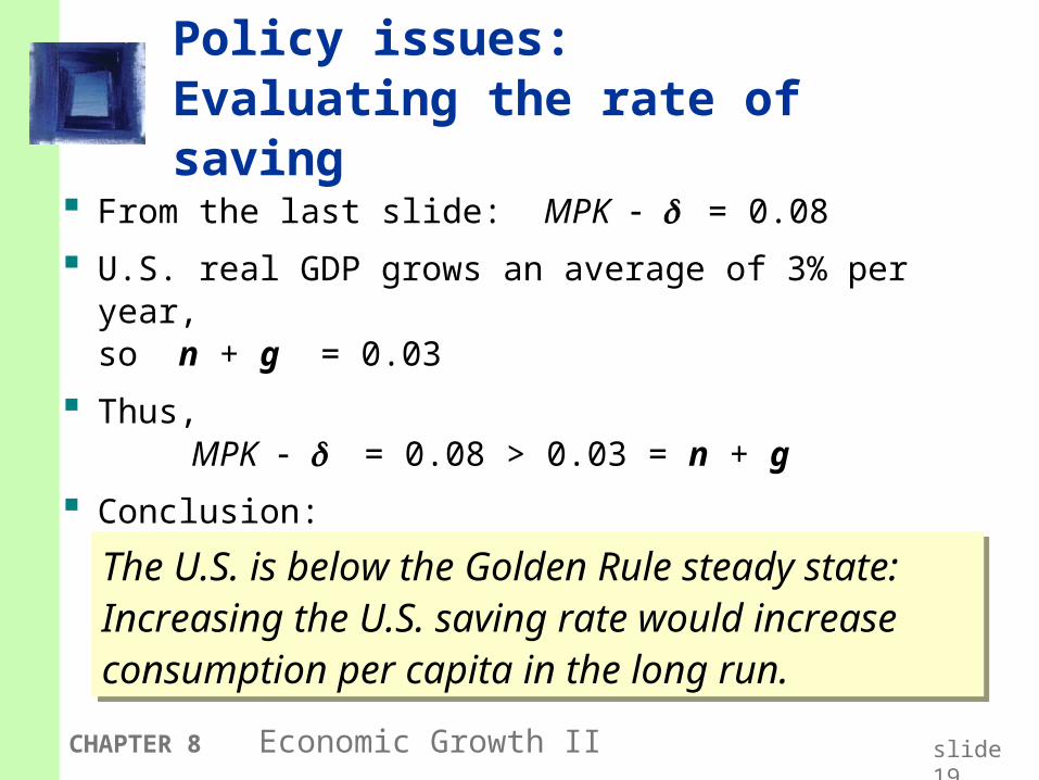
Policy issues: Evaluating the rate of saving
From the last slide: MPK = 0.08
U.S. real GDP grows an average of 3% per year, so n + g = 0.03
Thus, MPK = 0.08 > 0.03 = n + g
Conclusion:
The U.S. is below the Golden Rule steady state: Increasing the U.S. saving rate would increase consumption per capita in the long run.
The U.S. is below the Golden Rule steady state: Increasing the U.S. saving rate would increase consumption per capita in the long run.

CHAPTER 8 Economic Growth II slide 20
Policy issues: How to increase the saving rate
Reduce the government budget deficit(or increase the budget surplus).
Increase incentives for private saving: reduce capital gains tax, corporate income tax,
estate tax as they discourage saving. replace federal income tax with a consumption
tax. expand tax incentives for IRAs (individual
retirement accounts) and other retirement savings accounts.

CHAPTER 8 Economic Growth II slide 21
Policy issues: Allocating the economy’s investment
In the Solow model, there’s one type of capital.
In the real world, there are many types,which we can divide into three categories: private capital stock public infrastructure human capital: the knowledge and skills that
workers acquire through education.
How should we allocate investment among these types?

CHAPTER 8 Economic Growth II slide 22
Policy issues: Allocating the economy’s investment
Two viewpoints:
1. Equalize tax treatment of all types of capital in all industries, then let the market allocate investment to the type with the highest marginal product.
2. Industrial policy: Govt should actively encourage investment in capital of certain types or in certain industries, because they may have positive externalities that private investors don’t consider.

CHAPTER 8 Economic Growth II slide 23
Policy issues: Establishing the right institutions
Creating the right institutions is important for ensuring that resources are allocated to their best use. Examples:
Legal institutions, to protect property rights.
Capital markets, to help financial capital flow to the best investment projects.
A corruption-free government, to promote competition, enforce contracts, etc.
CHAPTER 8 Economic Growth II slide 24
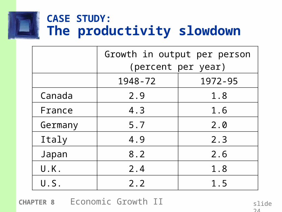
CASE STUDY: The productivity slowdown
1.5
1.8
2.6
2.3
2.0
1.6
1.8
2.2
2.4
8.2
4.9
5.7
4.3
2.9
1972-951948-72
U.S.
U.K.
Japan
Italy
Germany
France
Canada
Growth in output per person(percent per year)
CHAPTER 8 Economic Growth II slide 25
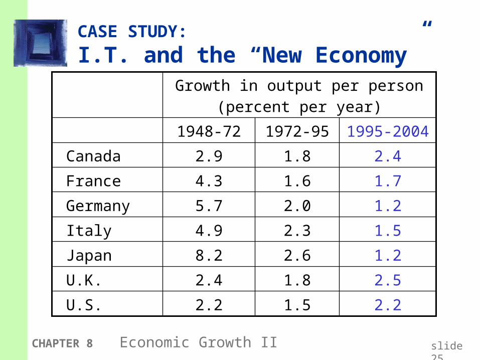
CASE STUDY:
I.T. and the “New Economy”
2.2
2.5
1.2
1.5
1.2
1.7
2.4
1.5
1.8
2.6
2.3
2.0
1.6
1.8
2.2
2.4
8.2
4.9
5.7
4.3
2.9
1995-20041972-951948-72
U.S.
U.K.
Japan
Italy
Germany
France
Canada
Growth in output per person(percent per year)

CHAPTER 8 Economic Growth II slide 26
CASE STUDY:
I.T. and the “New Economy”Apparently, the computer revolution did not affect aggregate productivity until the mid-1990s.
Two reasons:
1. Computer industry’s share of GDP much bigger in late 1990s than earlier.
2. Takes time for firms to determine how to utilize new technology most effectively.
The big, open question: How long will I.T. remain an engine of growth?
CHAPTER 8 Economic Growth II slide 27
Endogenous growth theory
Solow model: sustained growth in living standards is due to
tech progress. the rate of tech progress is exogenous.
Endogenous growth theory: a set of models in which the growth rate of
productivity and living standards is endogenous.
CHAPTER 8 Economic Growth II slide 28
A basic model
Production function: Y = A Kwhere A is the amount of output for each unit of capital (A is exogenous & constant)
Key difference between this model & Solow: MPK is constant here, diminishes in Solow
Investment: s Y
Depreciation: K
Equation of motion for total capital: K = s Y K
CHAPTER 8 Economic Growth II slide 29
A basic model
K = s Y K
Y KsA
Y K
If s A > , then income will grow forever, and investment is the “engine of growth.”
Here, the permanent growth rate depends on s. In Solow model, it does not.
Divide through by K and use Y = A K to get:
CHAPTER 8 Economic Growth II slide 30
Does capital have diminishing returns or not?
Depends on definition of “capital.”
If “capital” is narrowly defined (only plant & equipment), then yes.
Advocates of endogenous growth theory argue that knowledge is a type of capital.
If so, then constant returns to capital is more plausible, and this model may be a good description of economic growth.
CHAPTER 8 Economic Growth II slide 31
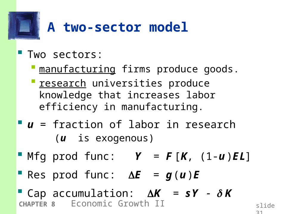
A two-sector model
Two sectors: manufacturing firms produce goods. research universities produce knowledge that
increases labor efficiency in manufacturing.
u = fraction of labor in research (u is exogenous)
Mfg prod func: Y = F [K, (1-u )E L]
Res prod func: E = g (u )E
Cap accumulation: K = s Y K

CHAPTER 8 Economic Growth II slide 32
A two-sector model
In the steady state, mfg output per worker and the standard of living grow at rate E/E = g (u ).
Key variables:s: affects the level of income, but not its
growth rate (same as in Solow model)u: affects level and growth rate of income
Question: Would an increase in u be unambiguously good for the economy?
CHAPTER 8 Economic Growth II slide 33
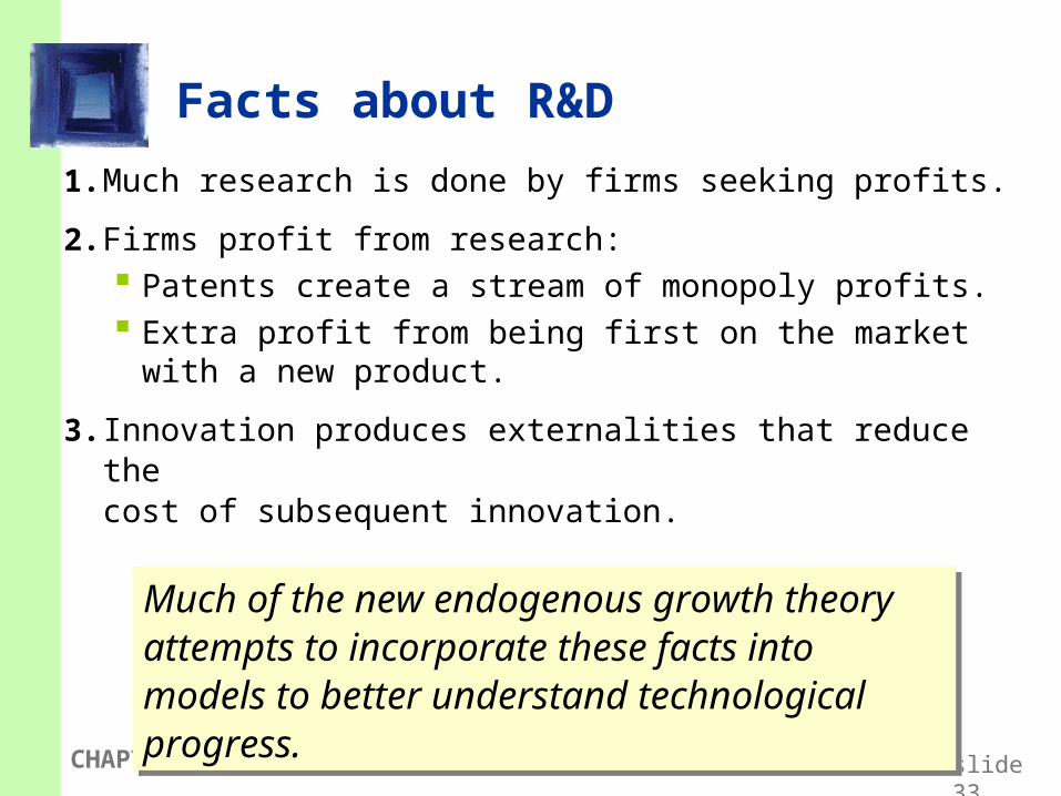
Facts about R&D
1. Much research is done by firms seeking profits.
2. Firms profit from research: Patents create a stream of monopoly profits. Extra profit from being first on the market with a
new product.
3. Innovation produces externalities that reduce the cost of subsequent innovation.
Much of the new endogenous growth theory attempts to incorporate these facts into models to better understand technological progress.
Much of the new endogenous growth theory attempts to incorporate these facts into models to better understand technological progress.
Chapter SummaryChapter Summary
1. Key results from Solow model with tech progress steady state growth rate of income per person
depends solely on the exogenous rate of tech progress
the U.S. has much less capital than the Golden Rule steady state
2. Ways to increase the saving rate increase public saving (reduce budget deficit) tax incentives for private saving
CHAPTER 8 Economic Growth II slide 34
Chapter SummaryChapter Summary
3. Productivity slowdown & “new economy” Early 1970s: productivity growth fell in the U.S.
and other countries. Mid 1990s: productivity growth increased,
probably because of advances in I.T.
4. Empirical studies Solow model explains balanced growth,
conditional convergence Cross-country variation in living standards is
due to differences in cap. accumulation and in production efficiency
CHAPTER 8 Economic Growth II slide 35
Chapter SummaryChapter Summary
5. Endogenous growth theory: Models that examine the determinants of the rate of
tech. progress, which Solow takes as given. explain decisions that determine the creation of
knowledge through R&D.
CHAPTER 8 Economic Growth II slide 36
MMACROECONOMICSACROECONOMICS
C H A P T E R
Introduction to Economic Fluctuations
9
CHAPTER 8 Economic Growth II slide 38
In this chapter, you will learn…
facts about the business cycle
how the short run differs from the long run
an introduction to aggregate demand
an introduction to aggregate supply in the short run and long run
how the model of aggregate demand and aggregate supply can be used to analyze the short-run and long-run effects of “shocks.”
CHAPTER 8 Economic Growth II slide 39
Facts about the business cycle
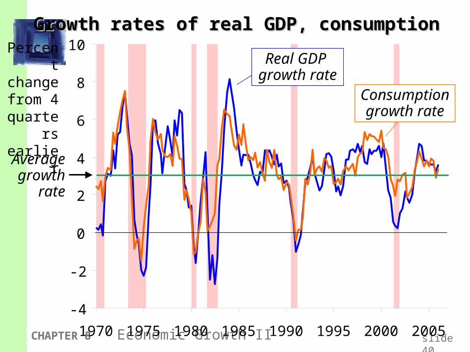
GDP growth averages 3–3.5 percent per year over the long run with large fluctuations in the short run.
Consumption and investment fluctuate with GDP, but consumption tends to be less volatile and investment more volatile than GDP.
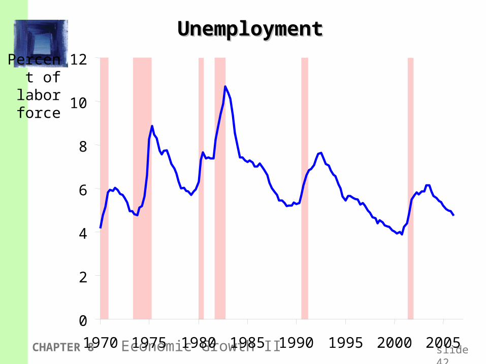
Unemployment rises during recessions and falls during expansions.
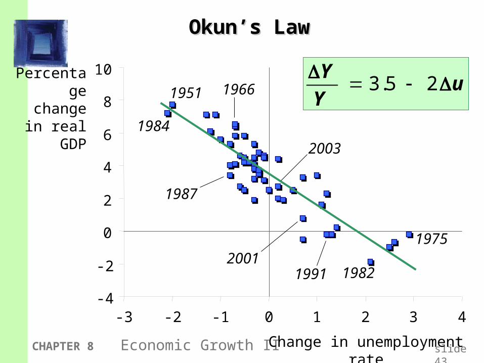
Okun’s Law: the negative relationship between GDP and unemployment.
CHAPTER 8 Economic Growth II slide 40
Growth rates of real GDP, consumptionGrowth rates of real GDP, consumption
-4
-2
0
2
4
6
8
10
1970 1975 1980 1985 1990 1995 2000 2005
Real GDP growth rate
Average growth
rate
Consumption growth rate
Percent change from 4
quarters earlier

CHAPTER 8 Economic Growth II slide 41
Growth rates of real GDP, consumption, investmentGrowth rates of real GDP, consumption, investment
-30
-20
-10
0
10
20
30
40
1970 1975 1980 1985 1990 1995 2000 2005
Percent change from 4
quarters earlier
Investment growth rate
Real GDP growth rate
Consumption growth rate
CHAPTER 8 Economic Growth II slide 42
UnemploymentUnemployment
0
2
4
6
8
10
12
1970 1975 1980 1985 1990 1995 2000 2005
Percent of labor
force
CHAPTER 8 Economic Growth II slide 43
Okun’s LawOkun’s Law
Percentage change in real GDP
Change in unemployment rate
-4
-2
0
2
4
6
8
10
-3 -2 -1 0 1 2 3 4
1975
198219912001
1984
1951 1966
2003
1987
3.5 2
Y
uY
CHAPTER 8 Economic Growth II slide 44
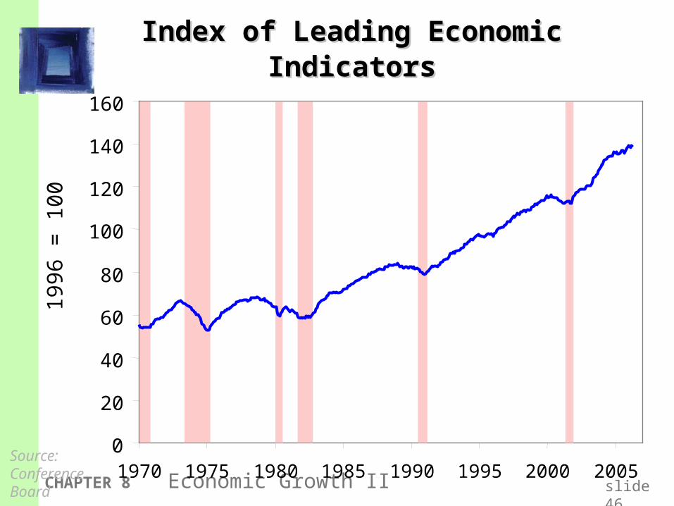
Index of Leading Economic Indicators
Published monthly by the Conference Board.
Aims to forecast changes in economic activity 6-9 months into the future.
Used in planning by businesses and govt, despite not being a perfect predictor.
CHAPTER 8 Economic Growth II slide 45
Components of the LEI index
Average workweek in manufacturing
Initial weekly claims for unemployment insurance
New orders for consumer goods and materials
New orders, nondefense capital goods
Vendor performance
New building permits issued
Index of stock prices
M2
Yield spread (10-year minus 3-month) on Treasuries
Index of consumer expectations
CHAPTER 8 Economic Growth II slide 46
Index of Leading Economic IndicatorsIndex of Leading Economic Indicators
0
20
40
60
80
100
120
140
160
1970 1975 1980 1985 1990 1995 2000 2005
19
96
= 1
00
Source: Conference Board
CHAPTER 8 Economic Growth II slide 47
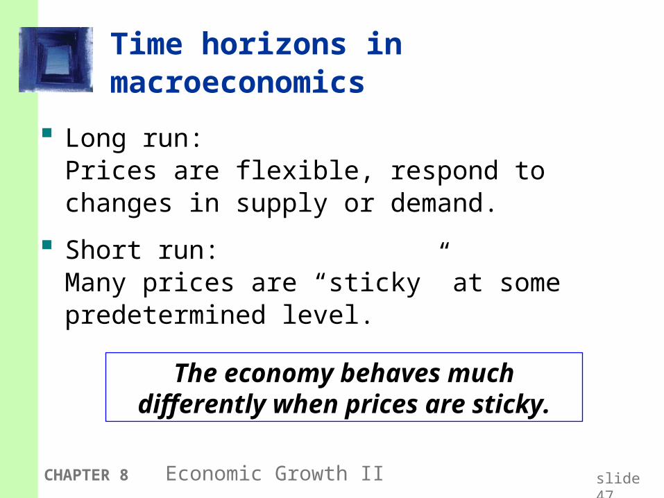
Time horizons in macroeconomics
Long run: Prices are flexible, respond to changes in supply or demand.
Short run:Many prices are “sticky” at some predetermined level.
The economy behaves much differently when prices are sticky.
CHAPTER 8 Economic Growth II slide 48
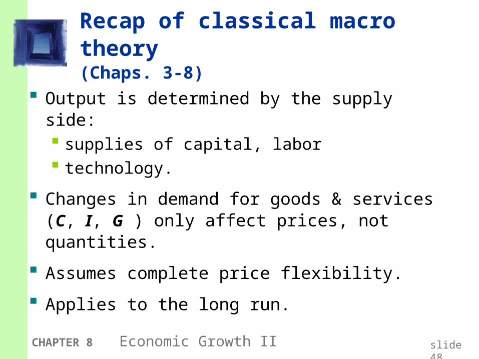
Recap of classical macro theory (Chaps. 3-8)
Output is determined by the supply side: supplies of capital, labor technology.
Changes in demand for goods & services (C, I, G ) only affect prices, not quantities.
Assumes complete price flexibility.
Applies to the long run.
CHAPTER 8 Economic Growth II slide 49
When prices are sticky…
…output and employment also depend on demand, which is affected by fiscal policy (G and T ) monetary policy (M ) other factors, like exogenous changes in
C or I.
CHAPTER 8 Economic Growth II slide 50
The Quantity Equation as Aggregate Demand
From Chapter 4, recall the quantity equation
M V = P Y
For given values of M and V, this equation implies an inverse relationship between P and Y :
CHAPTER 8 Economic Growth II slide 51
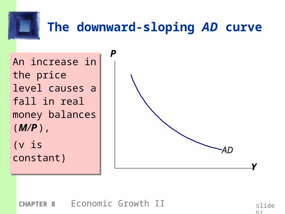
The downward-sloping AD curve
An increase in the price level causes a fall in real money balances (M/P ),
(v is constant)
An increase in the price level causes a fall in real money balances (M/P ),
(v is constant)
Y
P
AD
CHAPTER 8 Economic Growth II slide 52
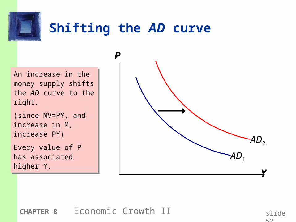
Shifting the AD curve
An increase in the money supply shifts the AD curve to the right.
(since MV=PY, and increase in M, increase PY)
Every value of P has associated higher Y.
An increase in the money supply shifts the AD curve to the right.
(since MV=PY, and increase in M, increase PY)
Every value of P has associated higher Y.
Y
P
AD1
AD2
CHAPTER 8 Economic Growth II slide 53
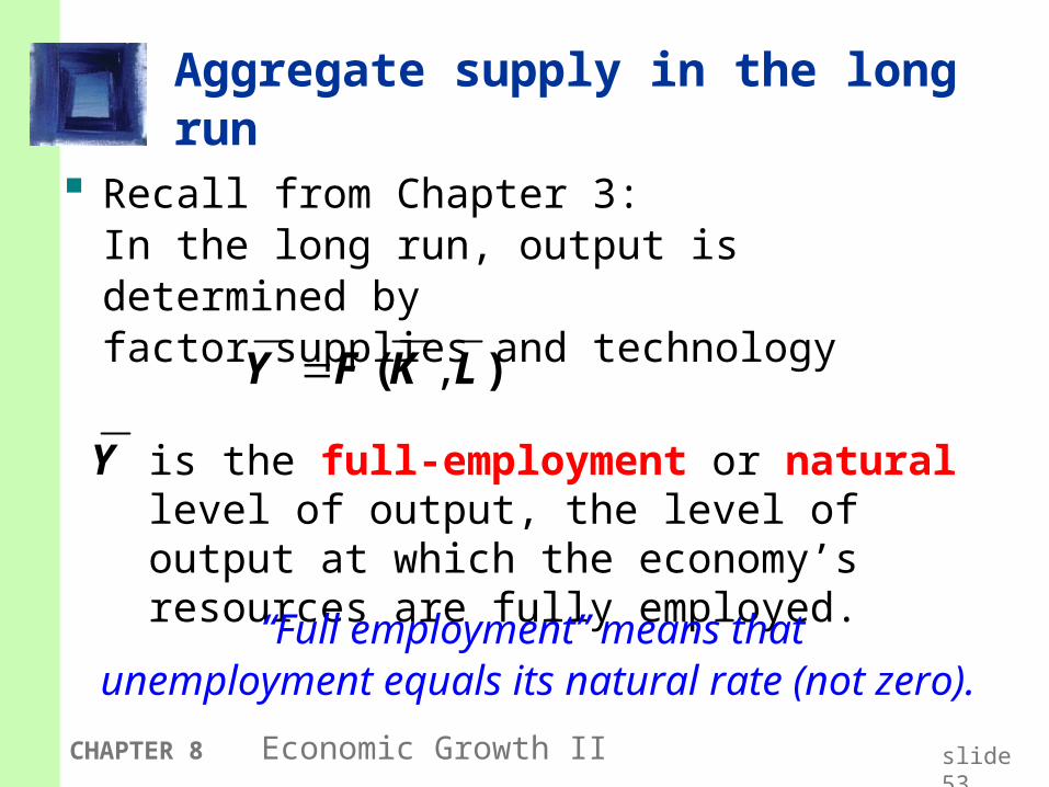
Aggregate supply in the long run
Recall from Chapter 3: In the long run, output is determined by factor supplies and technology
, ( )Y F K L
is the full-employment or natural level of output, the level of output at which the economy’s resources are fully employed.
Y
“Full employment” means that unemployment equals its natural rate (not zero).
CHAPTER 8 Economic Growth II slide 54
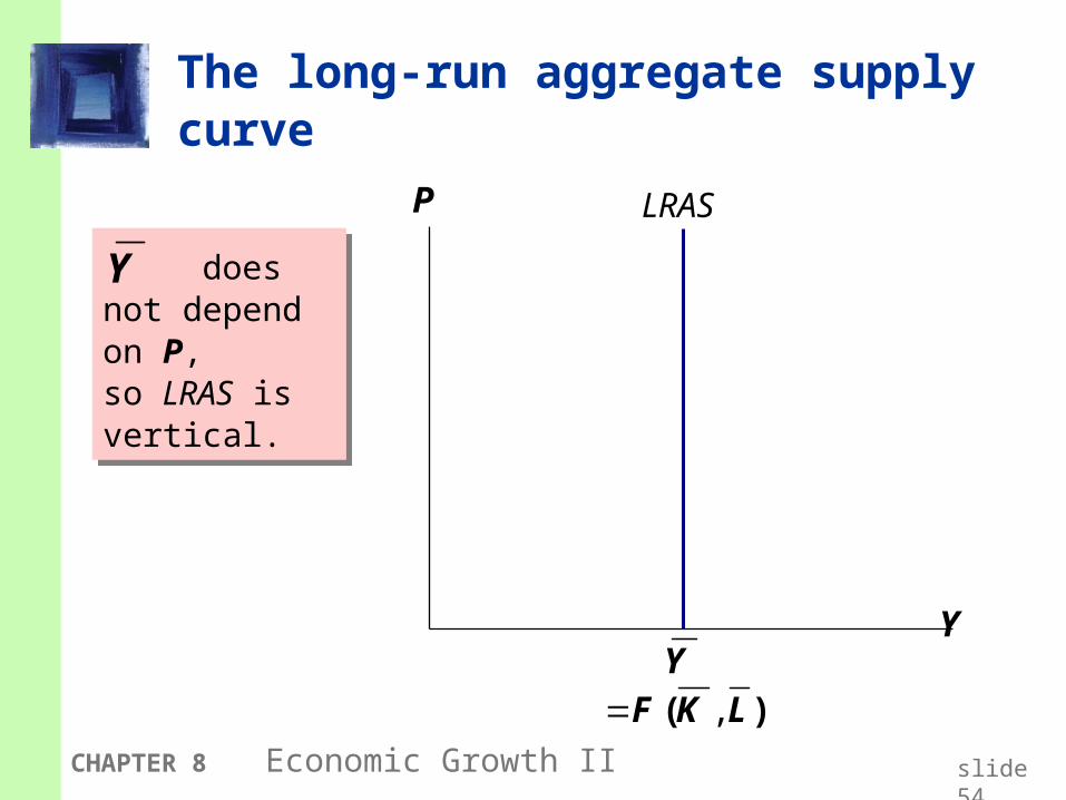
The long-run aggregate supply curve
Y
P LRAS
does not depend on P, so LRAS is vertical.
does not depend on P, so LRAS is vertical.
Y
( ) ,Y
F K L
CHAPTER 8 Economic Growth II slide 55
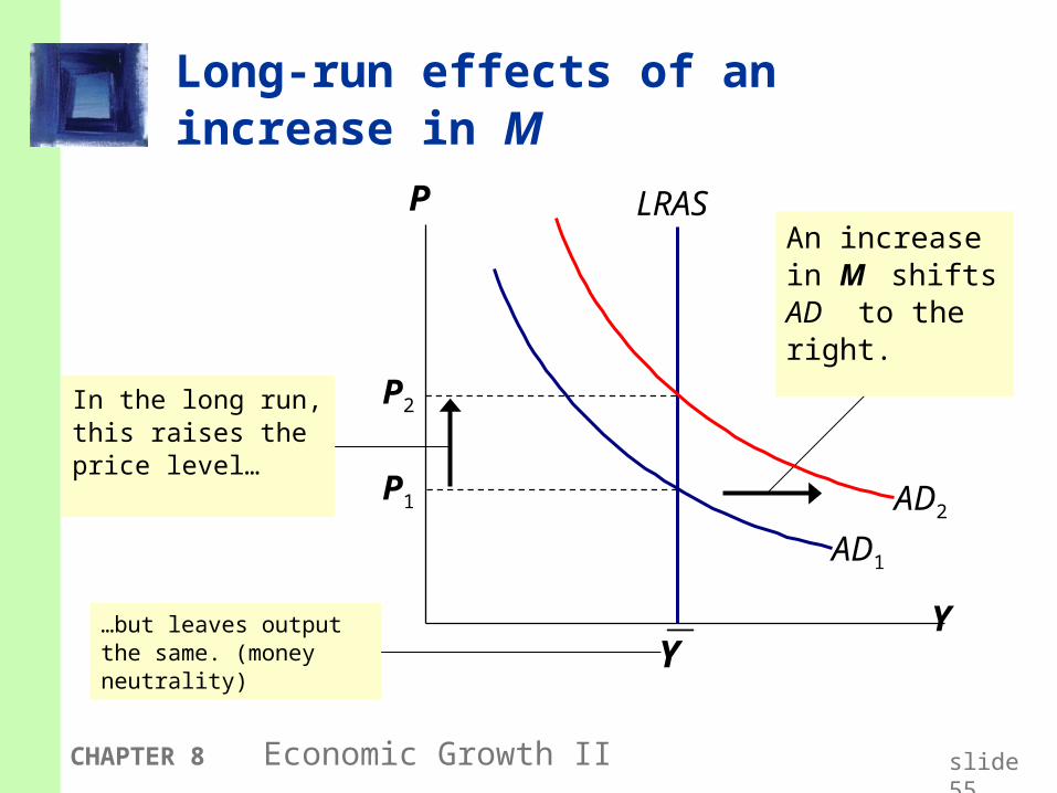
Long-run effects of an increase in M
Y
P
AD1
LRAS
Y
An increase in M shifts AD to the right.
P1
P2In the long run, this raises the price level…
…but leaves output the same. (money neutrality)
AD2
CHAPTER 8 Economic Growth II slide 56
Aggregate supply in the short run
Many prices are sticky in the short run.
For now (and through Chap. 12), we assume all prices are stuck at a predetermined level in
the short run. firms are willing to sell as much at that price
level as their customers are willing to buy.
Therefore, the short-run aggregate supply (SRAS) curve is horizontal:
CHAPTER 8 Economic Growth II slide 57
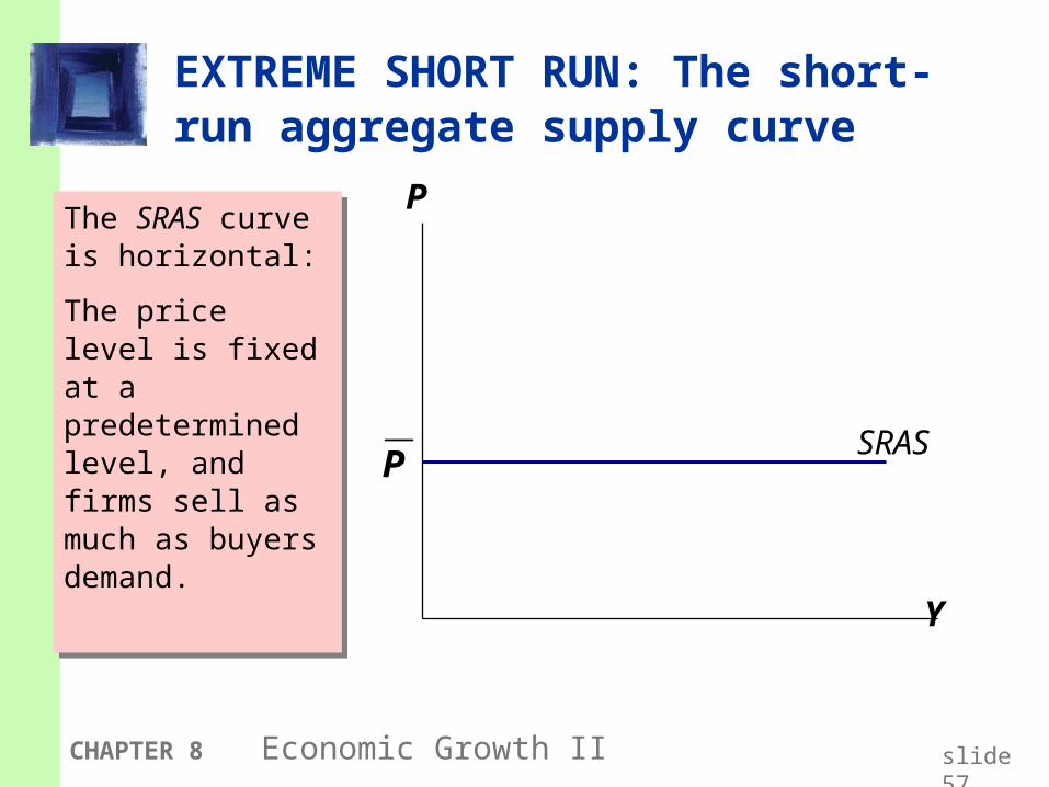
EXTREME SHORT RUN: The short-run aggregate supply curve
Y
P
PSRAS
The SRAS curve is horizontal:
The price level is fixed at a predetermined level, and firms sell as much as buyers demand.
The SRAS curve is horizontal:
The price level is fixed at a predetermined level, and firms sell as much as buyers demand.
CHAPTER 8 Economic Growth II slide 58
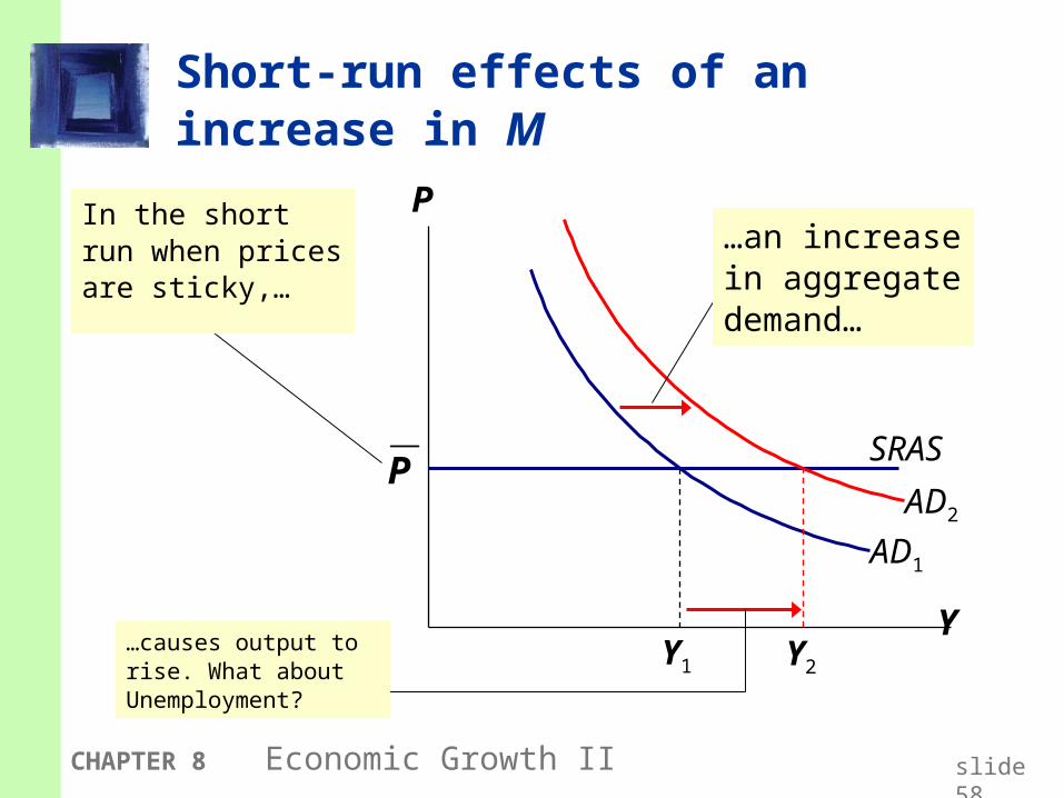
Short-run effects of an increase in M
Y
P
AD1
In the short run when prices are sticky,…
…causes output to rise. What about Unemployment?
PSRAS
Y2Y1
AD2
…an increase in aggregate demand…
CHAPTER 8 Economic Growth II slide 59
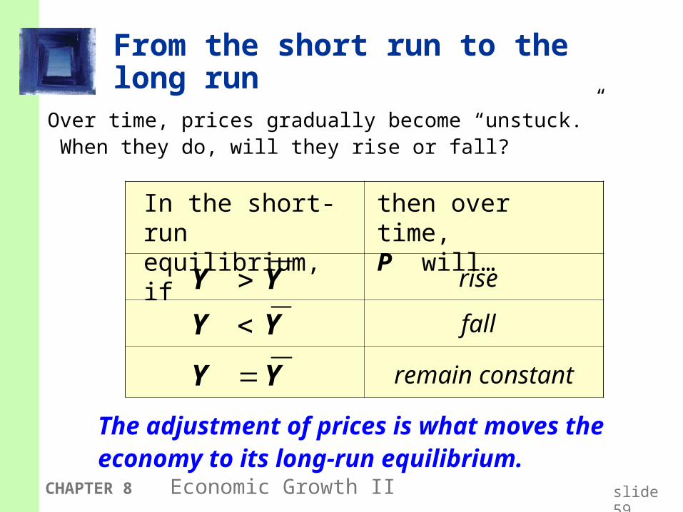
From the short run to the long run
Over time, prices gradually become “unstuck.” When they do, will they rise or fall?
Y Y
Y Y
Y Y
rise
fall
remain constant
In the short-run equilibrium, if
then over time, P will…
The adjustment of prices is what moves the economy to its long-run equilibrium.
CHAPTER 8 Economic Growth II slide 60
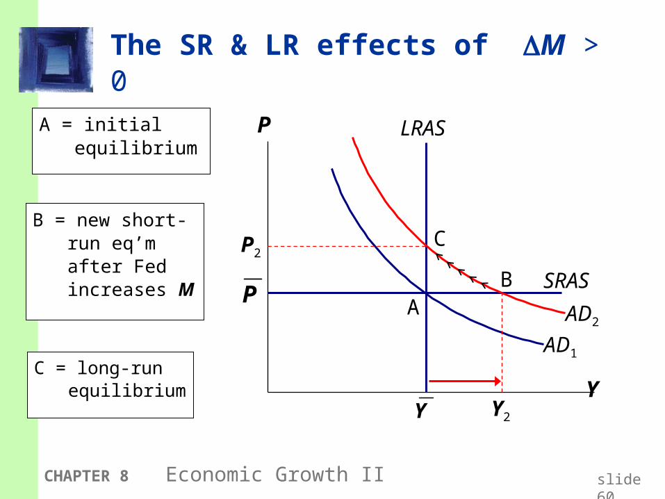
The SR & LR effects of M > 0
Y
P
AD1
LRAS
Y
PSRAS
P2
Y2
A = initial equilibrium
AB
CB = new short-
run eq’m after Fed increases M
C = long-run equilibrium
AD2
CHAPTER 8 Economic Growth II slide 61
How shocking!!!
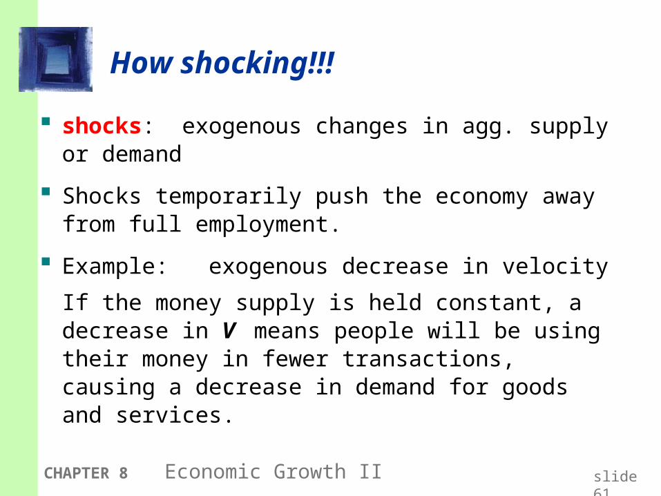
shocks: exogenous changes in agg. supply or demand
Shocks temporarily push the economy away from full employment.
Example: exogenous decrease in velocity
If the money supply is held constant, a decrease in V means people will be using their money in fewer transactions, causing a decrease in demand for goods and services.

CHAPTER 8 Economic Growth II slide 62
PSRAS
LRAS
AD2
The effects of a negative demand shock
Y
P
AD1
Y
P2
Y2
AD shifts left, depressing output and employment in the short run.
AD shifts left, depressing output and employment in the short run.
AB
C
Over time, prices fall and the economy moves down its demand curve toward full-employment.
Over time, prices fall and the economy moves down its demand curve toward full-employment.
CHAPTER 8 Economic Growth II slide 63
Supply shocks
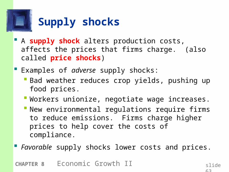
A supply shock alters production costs, affects the prices that firms charge. (also called price shocks)
Examples of adverse supply shocks: Bad weather reduces crop yields, pushing up
food prices. Workers unionize, negotiate wage increases. New environmental regulations require firms to
reduce emissions. Firms charge higher prices to help cover the costs of compliance.
Favorable supply shocks lower costs and prices.
CHAPTER 8 Economic Growth II slide 64
CASE STUDY: The 1970s oil shocks
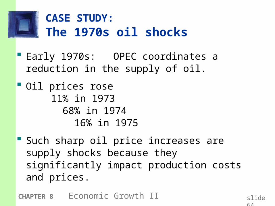
Early 1970s: OPEC coordinates a reduction in the supply of oil.
Oil prices rose11% in 1973 68% in 1974 16% in 1975
Such sharp oil price increases are supply shocks because they significantly impact production costs and prices.
CHAPTER 8 Economic Growth II slide 65
1P SRAS1
Y
P
AD
LRAS
YY2
CASE STUDY: The 1970s oil shocks
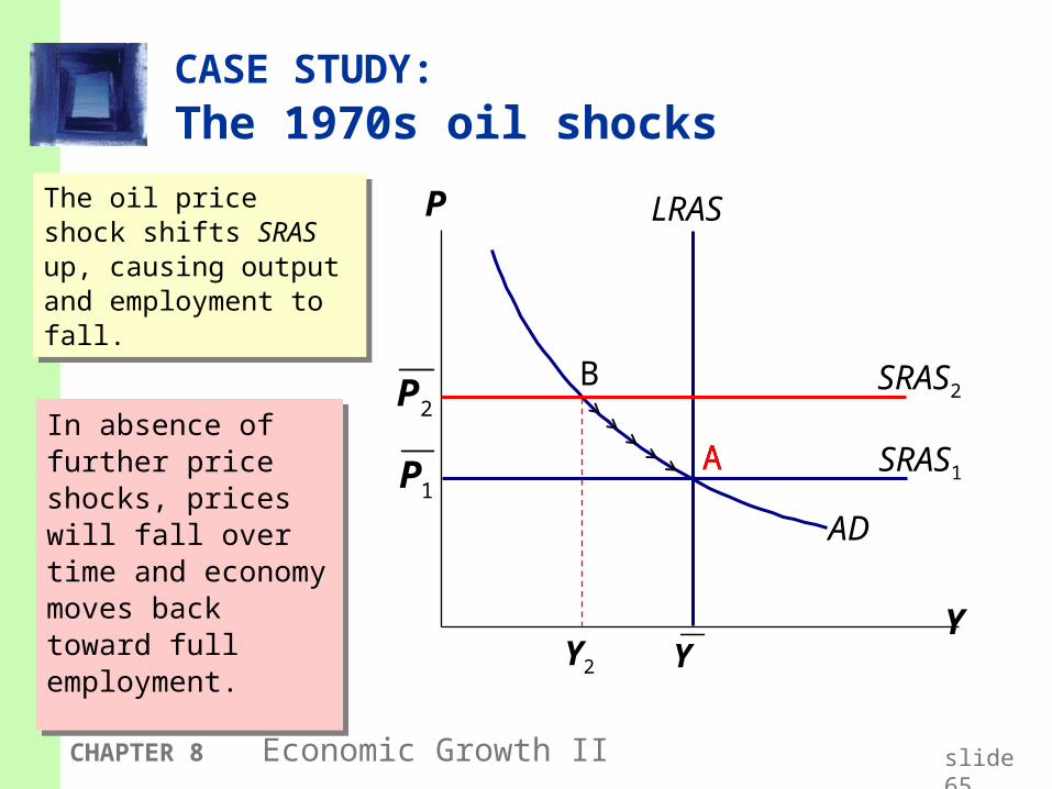
The oil price shock shifts SRAS up, causing output and employment to fall.
The oil price shock shifts SRAS up, causing output and employment to fall.
A
B
In absence of further price shocks, prices will fall over time and economy moves back toward full employment.
In absence of further price shocks, prices will fall over time and economy moves back toward full employment.
2P SRAS2
A
CHAPTER 8 Economic Growth II slide 66
Stabilization policy
def: policy actions aimed at reducing the severity of short-run economic fluctuations.
Example: Using monetary policy to combat the effects of adverse supply shocks:
CHAPTER 8 Economic Growth II slide 67
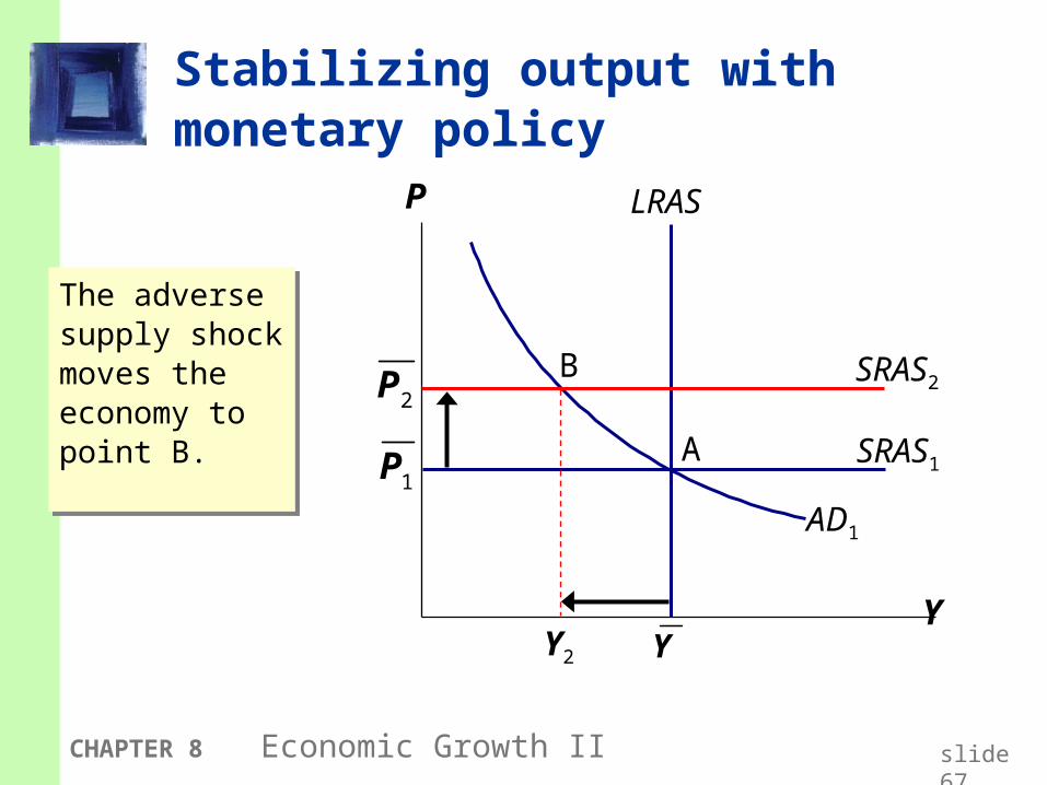
Stabilizing output with monetary policy
1P SRAS1
Y
P
AD1
B
A
Y2
LRAS
Y
The adverse supply shock moves the economy to point B.
The adverse supply shock moves the economy to point B.
2P SRAS2
CHAPTER 8 Economic Growth II slide 68
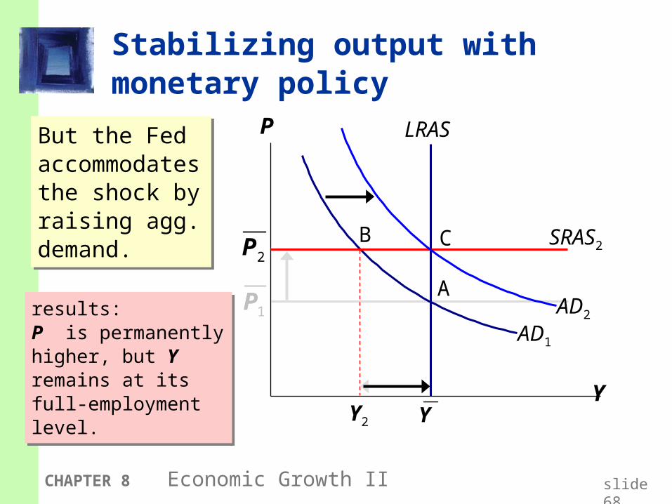
Stabilizing output with monetary policy
1P
Y
P
AD1
B
A
C
Y2
LRAS
Y
But the Fed accommodates the shock by raising agg. demand.
But the Fed accommodates the shock by raising agg. demand.
results: P is permanently higher, but Y remains at its full-employment level.
results: P is permanently higher, but Y remains at its full-employment level.
2P SRAS2
AD2
CHAPTER 8 Economic Growth II slide 69
Chapter SummaryChapter Summary
1. Long run: prices are flexible, output and employment are always at their natural rates, and the classical theory applies.
Short run: prices are sticky, shocks can push output and employment away from their natural rates.
2. Aggregate demand and supply: a framework to analyze economic fluctuations
CHAPTER 9 Introduction to Economic Fluctuations slide 69

CHAPTER 8 Economic Growth II slide 70
Chapter SummaryChapter Summary
3. The aggregate demand curve slopes downward.
4. The long-run aggregate supply curve is vertical, because output depends on technology and factor supplies, but not prices.
5. The short-run aggregate supply curve is horizontal, because prices are sticky at predetermined levels.
CHAPTER 9 Introduction to Economic Fluctuations slide 70
CHAPTER 8 Economic Growth II slide 71
Chapter SummaryChapter Summary
6. Shocks to aggregate demand and supply cause fluctuations in GDP and employment in the short run.
7. The Fed can attempt to stabilize the economy with monetary policy.
CHAPTER 9 Introduction to Economic Fluctuations slide 71
MMACROECONOMICSACROECONOMICS
C H A P T E R
Aggregate Demand I:Building the IS -LM Model
10
CHAPTER 8 Economic Growth II slide 73
In this chapter, you will learn…
the IS curve, and its relation to the Keynesian cross the loanable funds model
the LM curve, and its relation to the theory of liquidity preference
how the IS-LM model determines income and the interest rate in the short run when P is fixed
CHAPTER 8 Economic Growth II slide 74
Context
Chapter 9 introduced the model of aggregate demand and aggregate supply.
Long run prices flexible output determined by factors of production &
technology unemployment equals its natural rate
Short run prices fixed output determined by aggregate demand unemployment negatively related to output
CHAPTER 8 Economic Growth II slide 75
Context
This chapter develops the IS-LM model, the basis of the aggregate demand curve.
We focus on the short run and assume the price level is fixed (so, SRAS curve is horizontal).
This chapter (and chapter 11) focus on the closed-economy case. Chapter 12 presents the open-economy case.
CHAPTER 8 Economic Growth II slide 76
The Keynesian Cross
A simple closed economy model in which income is determined by expenditure. (due to J.M. Keynes)
Notation:
I = planned investment
E = C + I + G = planned expenditure
Y = real GDP = actual expenditure
Difference between actual & planned expenditure = unplanned inventory investment
CHAPTER 8 Economic Growth II slide 77
Elements of the Keynesian Cross
( )C C Y T
I I
,G G T T
( )E C Y T I G
Y E
consumption function:
for now, plannedinvestment is exogenous:
planned expenditure:
equilibrium condition:
govt policy variables:
actual expenditure = planned expenditure

CHAPTER 8 Economic Growth II slide 78
Graphing planned expenditure
income, output, Y
E
planned
expenditure
E =C +I +G
MPC1
CHAPTER 8 Economic Growth II slide 79
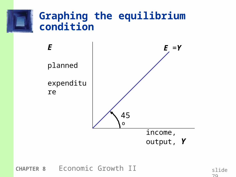
Graphing the equilibrium condition
income, output, Y
E
planned
expenditure
E =Y
45º
CHAPTER 8 Economic Growth II slide 80
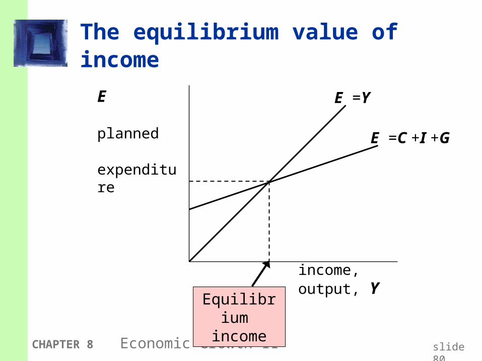
The equilibrium value of income
income, output, Y
E
planned
expenditure
E =Y
E =C +I +G
Equilibrium income

CHAPTER 8 Economic Growth II slide 81
An increase in government purchases
Y
E
E =Y
E =C +I +G1
E1 = Y1
E =C +I +G2
E2 = Y2Y
At Y1,
there is now an unplanned drop in inventory…
…so firms increase output, and income rises toward a new equilibrium.
G
CHAPTER 8 Economic Growth II slide 82
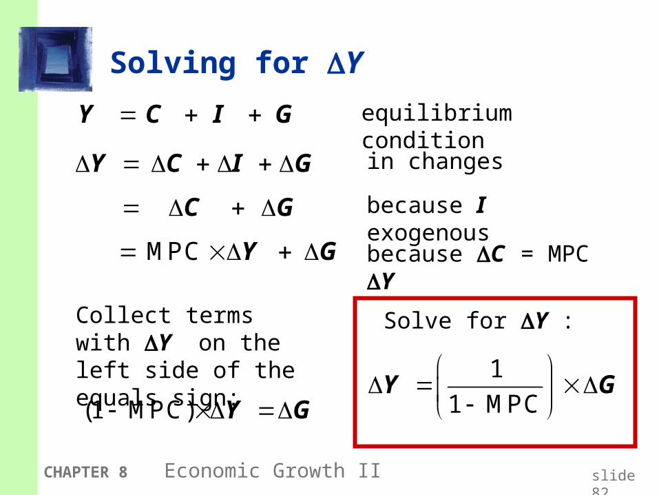
Solving for Y
Y C I G
Y C I G
MPC Y G
C G
(1 MPC) Y G
1
1 MPC
Y G
equilibrium condition
in changes
because I exogenous
because C = MPC
Y
Collect terms with Y on the left side of the equals sign:
Solve for Y :
CHAPTER 8 Economic Growth II slide 83
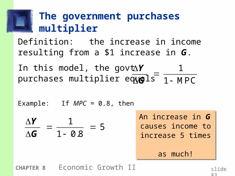
The government purchases multiplier
Example: If MPC = 0.8, then
Definition: the increase in income resulting from a $1 increase in G.
In this model, the govt purchases multiplier equals
1
1 MPC
YG
15
1 0.8
YG
An increase in G causes income to increase 5 times
as much!
An increase in G causes income to increase 5 times
as much!
CHAPTER 8 Economic Growth II slide 84
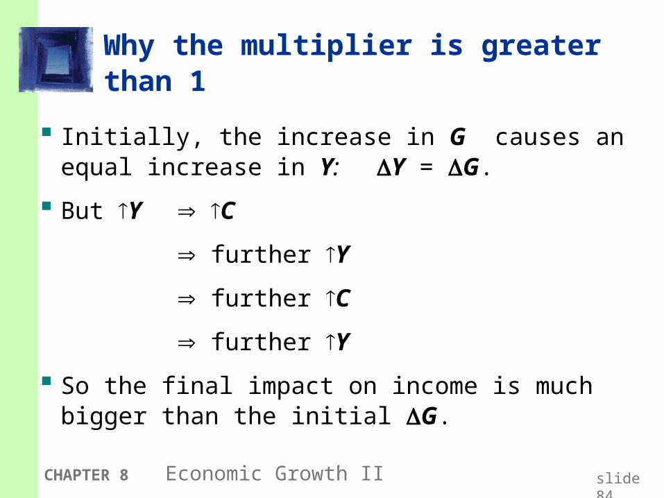
Why the multiplier is greater than 1
Initially, the increase in G causes an equal increase in Y: Y = G.
But Y C
further Y
further C
further Y
So the final impact on income is much bigger than the initial G.