1

Lyapunov Theory for Zeno StabilityAndrew Lamperski and Aaron D. Ames

Abstract—Zeno behavior is a dynamic phenomenon unique tohybrid systems in which an infinite number of discrete transitionsoccurs in a finite amount of time. This behavior commonlyarises in mechanical systems undergoing impacts and optimalcontrol problems, but its characterization for general hybridsystems is not completely understood. The goal of this paperis to develop a stability theory for Zeno hybrid systems thatparallels classical Lyapunov theory; that is, we present Lyapunov-like sufficient conditions for Zeno behavior obtained by mappingsolutions of complex hybrid systems to solutions of simpler Zenohybrid systems defined on the first quadrant of the plane. Theseconditions are applied to Lagrangian hybrid systems, whichmodel mechanical systems undergoing impacts, yielding simplesufficient conditions for Zeno behavior. Finally, the results areapplied to robotic bipedal walking.

I. INTRODUCTION

Zeno behavior occurs in hybrid systems when an execution(or solution) undergoes infinitely many discrete transitions ina finite amount of time. Prior to the introduction of hybridsystems, and in contrast with the view of Zeno behavior as amodeling pathology, Zeno phenomena have long been studiedin the fields of nonsmooth mechanics and optimal control.While understanding of Zeno behavior is, in these domains,quite sophisticated, many basic problems in the theory of Zenobehavior of general hybrid systems remain unsolved.

This paper studies the connections between Zeno behaviorand Lyapunov stability. In classical dynamical systems, sta-bility is a property of the asymptotic behavior of trajectoriesas time goes to infinity. In the model of hybrid systems usedin this paper, time is measured with two variables, one forreal time and the other for the number of discrete transitions.Zeno stability is a hybrid analog of classical stability in thecase that real time stays bounded, while the number of discretetransitions approaches infinity.

A. Summary of Contributions

The contributions of this paper are: 1) a theorem connectingasymptotic Zeno stability and the geometry of Zeno equilibria;2) Lyapunov-like sufficient conditions for local Zeno stabilityfor hybrid systems over cycles; 3) easily verifiable sufficientconditions for Zeno stability of Lagrangian hybrid systems,which model mechanical systems undergoing impacts.

Our first contribution deals with geometry of special in-variant sets, termed Zeno equilibria, which are analogous toequilibrium points of dynamical systems. A Zeno equilibriumis a set of points (with one point in each discrete domain)

A. Lamperski is with Control and Dynamical Systems atthe California Institute of Technology, Pasadena, CA 91125.andyl@cds.caltech.edu

A. D. Ames is with the Mechanical Engineering Department at Texas A&MUniversity, College Station, TX 77843. aames@tamu.edu

that is invariant under the discrete dynamics of the hybridsystem but not the continuous dynamics. Our result showsthat a Zeno equilibrium is asymptotically Zeno stable if andonly if it is isolated (each point in each domain is isolated).This result clarifies the limitations of existing results, [1], [2],[3], [4], [5], which focus either on isolated Zeno equilibriaor asymptotic convergence. In particular, their application toLagrangian systems with impacts (such as bouncing balls)is restricted to systems with one-dimensional configurationmanifolds, as higher-dimensional systems cannot have isolatedZeno equilibria [2].

The next contribution, which is the main result of thepaper, consists of Lyapunov-like sufficient conditions for Zenostability that, in contrast to existing results, apply to bothisolated and non-isolated Zeno equilibria. The classical Lya-punov theorem uses a Lyapunov function to map solutionsof a complex differential equation down to the solutionof a simple one-dimensional differential inclusion, and thenuses the structure of the Lyapunov function to prove thatthe original system inherits the stability properties of theone-dimensional system. Our approach to Zeno stability issimilarly inspired. We use Lyapunov-like functions to mapexecutions of a complex hybrid systems down to executions ofsimple two-dimensional differential inclusion hybrid systems,and then use the structure of the Lyapunov-like functions toprove that the original system inherits Zeno stability propertiesof the two-dimensional system.

Our final contribution applies the Lyapunov-like theorem toLagrangian hybrid systems (which model mechanical systemsundergoing impacts). Note that our Lyapunov-like theorem canbe applied to Lagrangian hybrid systems precisely becauseit applies equally well to isolated and non-isolated Zenoequilibria. While the technical machinery of hybrid systemsis not needed to develop the theory of mechanical systemswith impacts, we feel that any reasonable stability theory ofhybrid systems ought to cover this important special case.To prove Zeno stability in Lagrangian hybrid systems, wegive a general form for a Lyapunov-like function that appliesto any Lagrangian hybrid system whose vector field satisfiessimple algebraic conditions at a single point (based upon theunilateral constraint function defining the discrete componentof the Lagrangian hybrid system). Finally, it is shown how theresult can be used in robotic bipedal walking.

B. Relationship with Previous Results

As noted above, Zeno behavior has long been studied inoptimal control and nonsmooth mechanics. In 1960, Fullershowed that for certain constrained optimal control problems,the optimal controller makes an infinite number of switchesin a finite amount of time [6]. Since then, this phenomenon

2

has been observed and exploited in several optimal controlproblems [7]. In mechanics, Zeno behavior arising from im-pacts at the transition from bouncing to sliding is commonlyobserved [8]. While Zeno behavior can stall hybrid systemsimulations, time-stepping schemes for numerically integratingmechanical systems circumvent these problems because theydo not require that impact times and locations be explicitlycalculated [9]. Sufficient conditions for Zeno behavior, similarto the conditions for mechanical systems derived in thispaper are given in [10], [11]. Conditions to rule out Zenobehavior have also been given for linear complementaritysystems [12], [13], which are special hybrid models definedto capture discontinuous effects from nonsmooth mechanics,optimal control, and electrical circuits with diodes.

For hybrid systems, as studied in this paper, the theory ofZeno behavior has steadily matured with increased study ofthe dynamical aspects of hybrid systems. Hybrid automata, theprecursors of the systems of this paper, were originally intro-duced to reason about embedded computing systems. Since acomputer can only execute a finite number of operations ina finite amount of time, Zeno behavior was not allowed inearly definitions of executions of hybrid automata [14], [15],[16]. As the scope of hybrid automaton research was extendedto systems with rich continuous dynamics, attention to Zenobehavior increased to reason about well known examplessuch as the bouncing ball and Fuller’s phenomenon. Earlyresults focused on ruling out Zeno behavior using structuralconditions [17], [18], or proving its existence using closedform solutions to simple differential equations [19], [20].

With increasing development of the qualitative, geometrictheory hybrid systems [21], [22], connections between Zenobehavior and stability were recognized [23]. In [2], we gaveLyapunov-like sufficient conditions for asymptotic Zeno sta-bility of isolated Zeno equilibria in a class of systems similarto that studied in this paper. This work was generalized intwo separate directions in [24] and [4]. As mentioned above,Lagrangian hybrid systems with isolated Zeno equilibria musthave one-dimensional configuration manifolds. The aim of[24], on which the current paper is based, was to extendthe Lyapunov-like theory of Zeno stability to cover morecomplex examples, especially from mechanics, which typicallyhave non-isolated Zeno equilibria. The results on Lagrangianhybrid systems from [24] were subsequently extended andrefined in [25], [26], [27], [28], [29]. On the other hand, workin [4] exploited the connections between Zeno behavior andfinite-time stability to give Lyapunov theorems (and associatedconverse theorems) for asymptotic Zeno stability general classhybrid systems which encompasses the models considered in[2], [24], and the current paper. Note, however, that becausetheir work deals with asymptotic stability, it also cannot applyto nontrivial mechanical systems.

Similar to linearization in classical stability theory, Zenostability can also be studied with local approximations [1],[3], [5]. In particular, the connection between Zeno behaviorand homogeneity from [3], [5] was implicit in the early workof Fuller [6] and more fully explored subsequent work onoptimal control [7] and relay systems [30].

II. HYBRID SYSTEMS & ZENO BEHAVIOR

In this section, we introduce the basic terminology usedthroughout paper. That is, we define hybrid systems, execu-tions, and Zeno behavior. We study a restricted class of hybridautomata that strips away the nondeterminism and complicatedgraph structures allowing us to focus on consequences of thecontinuous dynamics.

Definition 1: A hybrid system on a cycle is a tuple:

H = (Γ, D,G,R, F ),

where• Γ = (Q,E) is a directed cycle, with

Q = {q0, . . . , qk−1},E = {e0 = (q0, q1), e1 = (q1, q2),

. . . , ek−1 = (qk−1, q0)}.

We denote the source of an edge e ∈ E by source(e) andthe target of an edge by target(e).

• D = {Dq}q∈Q is a set of continuous domains, where Dq

is a smooth manifold.• G = {Ge}e∈E is a set of guards, where Ge ⊆ Dsource(e)

is an embedded submanifold of Dsource(e).• R = {Re}e∈E is a set of reset maps, where Re : Ge ⊆Dsource(e) → Dtarget(e) is a smooth map.

• F = {fq}q∈Q, where fq : Dq → TDq is a Lipschitzvector field on Dq .

Remark 1: Note that if a hybrid system over a finite graphdisplays Zeno behavior, the graph must contain a cycle (see[17] and [18]). Therefore, beginning with hybrid systemsdefined on cycles greatly simplifies our analysis, while stillcapturing characteristic types of Zeno behavior.

Definition 2: An execution (or solution) of a hybrid systemH = (Γ, D,G,R, F ) is a tuple:

χ = (Λ, I, ρ, C)

where• Λ = {0, 1, 2, . . .} ⊆ N is a finite or infinite indexing set,• I = {Ii}i∈Λ where for each i ∈ Λ, Ii is defined as

follows: Ii = [τi, τi+1] if i, i + 1 ∈ Λ and IN−1 =[τN−1, τN ] or [τN−1, τN ) or [τN−1,∞) if |Λ| = N ,N finite. Here, for all i, i + 1 ∈ Λ, τi ≤ τi+1 withτi, τi+1 ∈ R, and τN−1 ≤ τN with τN−1, τN ∈ R. Weset τ0 = 0 for notational simplicity.

• ρ : Λ → Q is a map such that for all i, i + 1 ∈ Λ,(ρ(i), ρ(i + 1)) ∈ E. This is the discrete component ofthe execution.

• C = {ci}i∈Λ is a set of continuous trajectories, and theymust satisfy ci(t) = fρ(i)(ci(t)) for t ∈ Ii.

We require that when i, i+ 1 ∈ Λ,

(i) ci(t) ∈ Dρ(i) ∀ t ∈ Ii(ii) ci(τi+1) ∈ G(ρ(i),ρ(i+1))

(iii) R(ρ(i),ρ(i+1))(ci(τi+1)) = ci+1(τi+1).(1)

When i = |Λ| − 1, we still require that (i) holds.

3

We call c0(0) ∈ Dρ(0) the continuous initial condition andof χ. Likewise ρ(0) is the discrete initial condition of χ.

Remark 2: To ensure that executions are deterministic, it isassumed that when an execution reaches a guard, the transitionmust be taken. Furthermore, to ensure that executions can bedefined as t or i approach ∞, it is assumed that solutionsto x = fq(x) cannot leave Dq except through an associatedguard, Ge.

This paper studies Zeno executions, defined as follows:

Definition 3: An execution χ is Zeno if Λ = N and

limi→∞

τi =

∞∑i=0

τi+1 − τi = τ∞ <∞.

Here τ∞ is called the Zeno time.

Zeno behavior displays strong connections with Lyapunovstability [2], [4]. Just as classical stability focuses on equi-libria, much of the interesting Zeno behavior occurs near aspecial type of invariant set, termed Zeno equilibria.

Definition 4: A Zeno equilibrium of a hybrid system H =(Γ, D,G,R, F ) is a set z = {zq}q∈Q satisfying the followingconditions for all q ∈ Q:• For the unique edge e = (q, q′) ∈ E

– zq ∈ Ge,– Re(zq) = zq′ ,

• fq(zq) 6= 0.A Zeno equilibrium z = {zq}q∈Q is isolated if there is

a collection of open sets {Wq}q∈Q such that zq ∈ Wq ⊂Dq , and {Wq}q∈Q contains no Zeno equilibria other than z.Otherwise, z is non-isolated.

Note that, in particular, the conditions given in Definition 4imply that for all i ∈ {0, . . . , k − 1},

Rei−1◦ · · · ◦Re0 ◦Rek−1

◦ · · · ◦Rei(zi) = zi.

That is, the element zi is a fixed point under the reset mapscomposed in a cyclic manner. Furthermore, the assumptionsfrom Remark 2 imply that any infinite execution with initialcondition c0(0) ∈ z must be instantaneously Zeno (that is,τi = 0 for all i ∈ N).

Definition 4 captures notions that appear to be necessaryfor the Zeno phenomena studied in this paper. Indeed, unlessthe domains have geometric pathologies such as cusps orthe vector fields are not locally Lipschitz, convergent, non-chattering Zeno executions (those with τi < τi+1 for infinitelymany i) must converge to a Zeno equilibrium; see [21]Proposition 4.4. See [21] and [4] for examples of Zeno hybridsystems defined on cusps which do not have Zeno equilibria.

Finally, we give definitions that connect Zeno behavior toLyapunov stability.

Definition 5: An execution χ = (Λ, I, ρ, C) is maximal iffor all executions χ = (Λ, I, ρ, C) such that

Λ ⊂ Λ,⋃j∈Λ

Ij ⊂⋃j∈Λ

Ij ,

and cj(t) = cj(t) for all j ∈ Λ and t ∈ Ij , it follows thatχ = χ.

Definition 6: A Zeno equilibrium z = {zq}q∈Q of a hybridsystem H = (Γ, D,G,R, F ) is:• bounded-time Zeno stable if for every collection of open

sets {Uq}q∈Q with zq ∈ Uq ⊂ Dq and every ε > 0,there is another collection of open sets {Wq}q∈Q withzq ∈ Wq ⊂ Uq such that if χ is a maximal executionwith c0(0) ∈ Wρ(0), then χ is Zeno with τ∞ < ε andci(t) ∈ Uρ(i) for all i ∈ N and all t ∈ I .

• bounded-time asymptotically Zeno stable if it is bounded-time Zeno stable and there is a collection of open sets{Wq}q∈Q such that zq ∈ Wq ⊂ Dq and every Zenoexecution χ = (Λ, I, ρ, C) with c0(0) ∈Wρ(0) convergesto z as i→∞. More precisely, for any collection of opensets {Uq}q∈Q with zq ∈ Uq ⊂ Dq , there is N ∈ N suchthat if i ≥ N , then ci(t) ∈ Uρ(i) for all t ∈ Ii.

• bounded-time non-asymptotically Zeno stable if it isbounded-time Zeno stable but not bounded-time asymp-totically Zeno stable.

The following structural fact shows that isolatedness of aZeno equilibrium dictates the type of Zeno stability propertiesit can display. While the theorem is independent of the mainresults of the paper, it clarifies the existing sufficient conditionsfor Zeno stability and adds context to our current work.

Theorem 1: Let z = {zq}q∈Q be a bounded-time Zenostable equilibrium. Then z is bounded-time asymptoticallyZeno stable if and only if z is isolated.

Note the sharp contrast between Theorem 1 and classicalstability theory. The standard theory of continuous dynamicalsystems focuses primarily on isolated equilibria without muchapparent conceptual loss. In Zeno hybrid systems, however, wemust consider non-isolated Zeno equilibria just to describe thenon-asymptotic analog of Lyapunov stability.

From the theorem, we learn that many of the recent suf-ficient conditions for Zeno stability have similar limitations,but for different reasons. The work in [3] and [4] requiresbounded-time asymptotic Zeno stability (or the stronger globalversion), while [1] and [2] assume that the hybrid systemsstudied have isolated Zeno equilibria. None of the conditionsin the papers listed above apply to the mechanical systems inthis paper, since they have non-isolated Zeno equilibria.

Proof: Let z be an isolated Zeno equilibrium. By continu-ity, there is a collection of bounded neighborhoods {Uq}q∈Qcontaining no Zeno equilibria other than z, such that for allq ∈ Q, zq ∈ Uq ⊂ Dq and fq(x) 6= 0 for all x ∈ Uq .From bounded-time local Zeno stability, there is anothercollection of neighborhoods {Wq}q∈Q such that all maximalexecutions with initial conditions in {Wq}q∈Q are all Zenoand never leave {Uq}q∈Q. Let χ be any maximal executionsuch that c0(0) ∈ {Wq}q∈Q. Since χ is Zeno and bounded,Proposition 4.3 of [21] implies that there is a collection ofpoints z = {zq}q∈Q such that:• zq ∈ G(q,q′) ∩ Uq for all (q, q′) ∈ E,

4

(a)

−1 −0.5 0 0.5 1 1.5

−1

−0.8

−0.6

−0.4

−0.2

0

0.2

0.4

0.6

0.8

1

(b)

−1 −0.5 0 0.5 1 1.5

−1

−0.8

−0.6

−0.4

−0.2

0

0.2

0.4

0.6

0.8

1

(c)

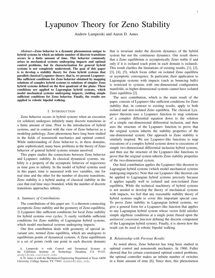
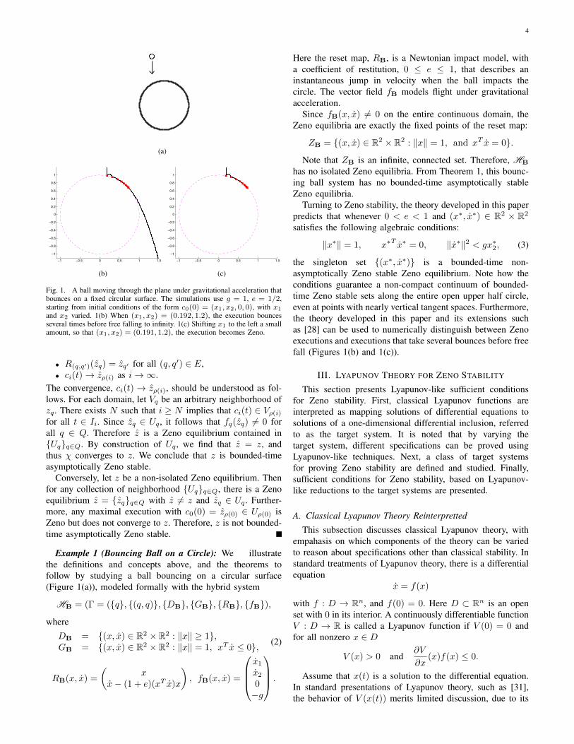
Fig. 1. A ball moving through the plane under gravitational acceleration thatbounces on a fixed circular surface. The simulations use g = 1, e = 1/2,starting from initial conditions of the form c0(0) = (x1, x2, 0, 0), with x1

and x2 varied. 1(b) When (x1, x2) = (0.192, 1.2), the execution bouncesseveral times before free falling to infinity. 1(c) Shifting x1 to the left a smallamount, so that (x1, x2) = (0.191, 1.2), the execution becomes Zeno.

• R(q,q′)(zq) = zq′ for all (q, q′) ∈ E,• ci(t)→ zρ(i) as i→∞.

The convergence, ci(t)→ zρ(i), should be understood as fol-lows. For each domain, let Vq be an arbitrary neighborhood ofzq . There exists N such that i ≥ N implies that ci(t) ∈ Vρ(i)for all t ∈ Ii. Since zq ∈ Uq , it follows that fq(zq) 6= 0 forall q ∈ Q. Therefore z is a Zeno equilibrium contained in{Uq}q∈Q. By construction of Uq , we find that z = z, andthus χ converges to z. We conclude that z is bounded-timeasymptotically Zeno stable.

Conversely, let z be a non-isolated Zeno equilibrium. Thenfor any collection of neighborhood {Uq}q∈Q, there is a Zenoequilibrium z = {zq}q∈Q with z 6= z and zq ∈ Uq . Further-more, any maximal execution with c0(0) = zρ(0) ∈ Uρ(0) isZeno but does not converge to z. Therefore, z is not bounded-time asymptotically Zeno stable.

Example 1 (Bouncing Ball on a Circle): We illustratethe definitions and concepts above, and the theorems tofollow by studying a ball bouncing on a circular surface(Figure 1(a)), modeled formally with the hybrid system

HB = (Γ = ({q}, {(q, q)}, {DB}, {GB}, {RB}, {fB}),

where

DB = {(x, x) ∈ R2 × R2 : ‖x‖ ≥ 1},GB = {(x, x) ∈ R2 × R2 : ‖x‖ = 1, xT x ≤ 0}, (2)

RB(x, x) =

(x

x− (1 + e)(xT x)x

), fB(x, x) =

x1

x2

0−g

.

Here the reset map, RB, is a Newtonian impact model, witha coefficient of restitution, 0 ≤ e ≤ 1, that describes aninstantaneous jump in velocity when the ball impacts thecircle. The vector field fB models flight under gravitationalacceleration.

Since fB(x, x) 6= 0 on the entire continuous domain, theZeno equilibria are exactly the fixed points of the reset map:

ZB = {(x, x) ∈ R2 × R2 : ‖x‖ = 1, and xT x = 0}.

Note that ZB is an infinite, connected set. Therefore, HB

has no isolated Zeno equilibria. From Theorem 1, this bounc-ing ball system has no bounded-time asymptotically stableZeno equilibria.

Turning to Zeno stability, the theory developed in this paperpredicts that whenever 0 < e < 1 and (x∗, x∗) ∈ R2 × R2

satisfies the following algebraic conditions:

‖x∗‖ = 1, x∗T x∗ = 0, ‖x∗‖2 < gx∗2, (3)

the singleton set {(x∗, x∗)} is a bounded-time non-asymptotically Zeno stable Zeno equilibrium. Note how theconditions guarantee a non-compact continuum of bounded-time Zeno stable sets along the entire open upper half circle,even at points with nearly vertical tangent spaces. Furthermore,the theory developed in this paper and its extensions suchas [28] can be used to numerically distinguish between Zenoexecutions and executions that take several bounces before freefall (Figures 1(b) and 1(c)).

III. LYAPUNOV THEORY FOR ZENO STABILITY

This section presents Lyapunov-like sufficient conditionsfor Zeno stability. First, classical Lyapunov functions areinterpreted as mapping solutions of differential equations tosolutions of a one-dimensional differential inclusion, referredto as the target system. It is noted that by varying thetarget system, different specifications can be proved usingLyapunov-like techniques. Next, a class of target systemsfor proving Zeno stability are defined and studied. Finally,sufficient conditions for Zeno stability, based on Lyapunov-like reductions to the target systems are presented.

A. Classical Lyapunov Theory Reinterpretted

This subsection discusses classical Lyapunov theory, withempahasis on which components of the theory can be variedto reason about specifications other than classical stability. Instandard treatments of Lyapunov theory, there is a differentialequation

x = f(x)

with f : D → Rn, and f(0) = 0. Here D ⊂ Rn is an openset with 0 in its interior. A continuously differentiable functionV : D → R is called a Lyapunov function if V (0) = 0 andfor all nonzero x ∈ D

V (x) > 0 and∂V

∂x(x)f(x) ≤ 0.

Assume that x(t) is a solution to the differential equation.In standard presentations of Lyapunov theory, such as [31],the behavior of V (x(t)) merits limited discussion, due to its

5

simplicity. To modify Lyapunov theory, however, the behaviorof the image V (x(t)) is crucial and will thus be emphasized.First note that V (x(t)) satisfies the following differentialinclusion on the non-negative real line:

v ∈{

(−∞, 0] for v > 0{0} for v = 0.

(4)

While V (x(t)) satisfies a differential inclusion, it typicallydoes not satisfy a differential equation because V and its Liederivative are typically not 1-1. In particular, it is often thecase that there are two vectors x and x such that

V (x) = V (x) but∂V

∂x(x)f(x) 6= ∂V

∂x(x)f(x).

The target system, defined by equation (4), encodes simplestable dynamics that are flexible enough to describe conver-gence properties of the orignal dynamical system, through theuse of a Lyapunov function. In a sense, the Lyapunov function“reduces” the stability properties of the original system to thestability properties of the target system. For Zeno stability,an analogous development holds. A simple class of hybridsystems is defined to serve as target systems. Then, Lyapunov-like functions are given to reduce Zeno stability properties of agiven hybrid system to the stability properties of the associatedtarget system.

B. First Quadrant Interval Hybrid Systems

This subsection introduces first quadrant interval hybrid sys-tems, which serve as the targets for Lyapunov-like reductionsfor Zeno stability. First quadrant interval hybrid systems area variant of first quadrant hybrid systems studied in [1] and[20]. We use the term “interval” since both the vector fieldsand reset maps are interval valued. See [32] and [33] for moreon set valued functions and differential inclusions.

Definition 7: A first quadrant interval (FQI) hybrid sys-tem is a tuple

HFQI = (Γ, D,G,R, F )

where• Γ = (Q,E) is a directed cycle as in Definition 1.• D = {Dq}q∈Q where for all q ∈ Q,

Dq = R2≥0 = {(x1, x2)T ∈ R2 : x1 ≥ 0, x2 ≥ 0}.

• G = {Ge}q∈Q where for all e ∈ E,

Ge = {(x1, x2)T ∈ R2≥0 : x1 = 0, x2 ≥ 0}.

• R = {Re}e∈E where for all e ∈ E, Re is a set valuedfunction defined by

Re(0, x2) = {(y1, y2)T ∈ Dq′ : y1 = 0,

y2 ∈ [γlex2, γue x2]},

for γue ≥ γle > 0 and for all (0, x2)T ∈ Ge.• F = {fq}q∈Q where for all q ∈ Q, fq is the (constant)

set-valued function defined by

fq(x) = {(y1, y2)T ∈ R2 : y1 ∈ [αlq, αuq ], y2 ∈ [βlq, β

uq ]}.

Definition 8: An execution of a first quadrant interval sys-tem, HFQI is a tuple χFQI = (Λ, I, ρ, C) where• Λ, I and ρ are defined as in Definition 2.• C = {ci}i∈Λ is a set of continuous trajectories that

satisfy the differential inclusion ci(t) ∈ fρ(i)(ci(t)) fort ∈ Ii.

We require that when i, i+ 1 ∈ Λ,

(i) ci(t) ∈ Dρ(i) ∀ t ∈ Ii(ii) ci(τi+1) ∈ G(ρ(i),ρ(i+1))

(iii) ci+1(τi+1) ∈ R(ρ(i),ρ(i+1))(ci(τi+1)).(5)

When i = |Λ| − 1, we still require that (i) holds.

As mentioned above, the class of first quadrant intervalhybrid systems is motivated by their simple Zeno stabilitytheory. Indeed, they are among the simplest systems that candemonstrate the non-chattering Zeno behavior of interest forthis paper. The following theorem gives sufficient conditionsfor Zeno stability of first quadrant interval hybrid systems.

Theorem 2: Let HFQI = (Γ, D,G,R, F ) be a first quad-rant interval hybrid system. If αuq < 0 < βlq for all q ∈ Q,γle > 0 for all e ∈ E and

|Q|−1∏i=0

∣∣∣∣γuei βuqiαuqi

∣∣∣∣ < 1

then the origin {0q}q∈Q is bounded-time asymptotically Zenostable.

Proof: Define 0 < ζ < 1 by

ζ :=

|Q|−1∏i=0

∣∣∣∣γuei βuqiαuqi

∣∣∣∣ . (6)

Let χFQI be an execution of HFQI . Without loss of gen-erality, assume that c0(0) ∈ Dq0 . Since fq(x)2 ≥ βlq > 0,the continuous trajectories travel upwards, away from the x1-axis. Likewise, fq(x)1 ≤ αuq < 0 implies that the continuoustrajectories travel left, towards the x2-axis. Therefore, byconstruction, events are always guaranteed to occur and we canassume that Λ = N. For simplicity, assume that c0(0)2 = 0.Dropping this assumption changes little, though the proofsbecome messier.

The hypothesis αuρ(i) < 0 implies that ci(t)1 ≤ ci(τi)1 +αuρ(i)(t− τi), and therefore

τi+1 − τi ≤

∣∣∣∣∣ci(τi)1

αuρ(i)

∣∣∣∣∣ , (7)

for all i ≥ 0. Given the assumption that c0(0)2 = 0 and thefact that ci(τi)2 = 0 for all i ≥ 1, the continuous state atevents must satisfy

ci(τi+1)2 ≤ βuρ(i)(τi+1 − τi) ≤ ci(τi)1

∣∣∣∣∣βuρ(i)

αuρ(i)

∣∣∣∣∣ . (8)

Thus, after the events the continuous state satisfies

ci+1(τi+1)1 ≤ γu(ρ(i),ρ(i+1))ci(τi+1)2

≤ ci(τi)1γu(ρ(i),ρ(i+1))

∣∣∣∣∣ βuρ(i)

αuρ(u)

∣∣∣∣∣ . (9)

6

Inductively combining the bounds from equation (9) gives abound in terms of c0(0)1:

ci(τi)1 ≤ c0(0)1

i−1∏j=0

∣∣∣∣∣γu(ρ(j),ρ(j+1))

βuρ(j)

αuρ(j)

∣∣∣∣∣ , (10)

for all i ≥ 0.To prove stability and asymptotic convergence note that

αuq < 0 < βlq implies that ci(t)1 ≤ ci(τi)1 and ci(t)2 ≤ci(τi+1)2 for all t ∈ Ii. Combining equations (8), (9), and(10) gives the bound

‖ci(t)‖≤ ci(τi)1 + ci(τi+1)2

≤

(1 +

∣∣∣∣∣βuρ(i)

αuρ(i)

∣∣∣∣∣)ci(τi)1

≤

(1 +

∣∣∣∣∣βuρ(i)

αuρ(i)

∣∣∣∣∣)c0(0)1

i−1∏j=0

∣∣∣∣∣γu(ρ(j),ρ(j+1))

βuρ(j)

αuρ(j)

∣∣∣∣∣Since the product in the last inequality converges to 0 as i→∞, executions with c0(0)1 small must remain near the origin,and ci(t)→ 0ρ(i) as i→∞.

Combining equations (6), (7) and (10) and proves that χ isZeno:

∞∑i=0

τi+1 − τi

≤ c0(0)1

∞∑i=0

1

|αuρ(i)|

i−1∏j=0

∣∣∣∣∣γu(ρ(j),ρ(j+1))

βuρ(j)

αuρ(j)

∣∣∣∣∣= c0(0)1

|Q|−1∑j=0

1

|αuqj |

j−1∏k=0

∣∣∣∣γuek βuqkαuqk

∣∣∣∣ ·( ∞∑

i=0

ζi

)< ∞.

Furthermore, note that the bound on the Zeno time goes tozero as c1(0)1 → 0.

Theorem 2 can also be proved using Lyapunov methodsfrom [4] or the homogeneity methods from [5], but the specificform of convergence of ci(t) to the Zeno equilibrium exploitedin the proof above is used to prove Theorem 3.

The Target Systems from [4]. It is worth comparing firstquadrant interval hybrid systems with the class of targets usedin [4]. These targets are defined for v ∈ [0,∞) by

v ∈{

(−∞,−1] for v > 00 for v = 0

v+ ∈ [0, v − κ(v)] for v ≥ 0,

where κ is some class K∞ function. In the framework of[4], solutions for this hybrid system flow according to thedifferential inclusion almost everywhere, but can make a jumpsaccording to the difference inclusion at nondeterministic times.If any such solution starts at v = v0, then it must converge to0 in time at most v0. Thus, these target systems exhibit finite-time convergence but the solutions may or may not be Zeno.To guarantee non-chattering Zeno behavior, extra conditionson the original hybrid system must be checked.

C. Sufficient Conditions for Zeno Stability Through Reductionto FQI Hybrid Systems

This subsection gives the main Lyapunov-type theorem ofthis paper. Our theorem uses special Lyapunov-like functionsto map executions of complex hybrid systems down to exe-cutions of FQI hybrid systems, thus transferring some Zenostability properties from Theorem 2. The theorem applies toboth isolated and non-isolated Zeno equilibria. Therefore, byTheorem 1, our sufficient conditions can imply bounded-timeasymptotic or non-asymptotic Zeno stability, depending on thetype of Zeno equilibrium in question.

Reduction conditions. Let z = {zq}q∈Q be a Zeno equi-librium (not necessarily isolated) of a hybrid system H =(Γ, D,G,R, F ), {Wq}q∈Q be a collection of open sets withzq ∈ Wq ⊆ Dq and {ψq}q∈Q be a collection of C1 maps;these are “Lyapunov-like” functions, with

ψq : Wq ⊆ Dq → R2≥0.

Consider the following conditions:

R1: ψq(zq) = 0 for all q ∈ Q.R2: If (q, q′) ∈ E, then ψq(x)1 = 0 if and only

if x ∈ G(q,q′) ∩Wq .R3: dψq(zq)1fq(zq) < 0 < dψq(zq)2fq(zq) for

all q ∈ Q.R4: ψq′(R(q,q′)(x))2 = 0 and there exist con-

stants 0 < γle ≤ γue such that

ψq′(R(q,q′)(x))1 ∈[γl(q,q′)ψq(x)2, γ

u(q,q′)ψq(x)2

]for all x ∈ G(q,q′) ∩Wq and all (q, q′) ∈ E.

R5:|Q|−1∏i=0

∣∣∣∣γuei dψqi(zqi)2fqi(zqi)

dψqi(zqi)1fqi(zqi)

∣∣∣∣ < 1.

R6: There exists K ≥ 0 such that

‖R(q,q′)(x)− zq′‖ ≤ ‖x− zq‖+Kψq(x)2

for all x ∈ G(q,q′) ∩Wq and all (q, q′) ∈ E.

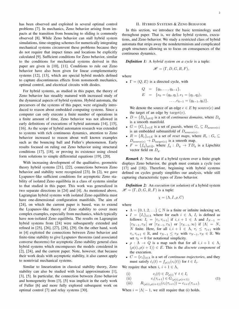
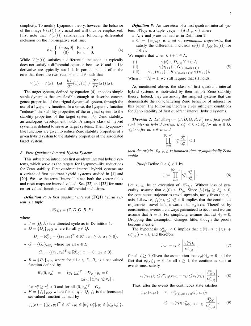
Remark 3: Just as the conditions on classical Lyapunovfunctions guarantee that solutions of a dynamical system canbe mapped to solutions of a stable one-dimensional system,conditions R1-R5 guarantee that ψq can be used to mapexecutions of H to executions of a Zeno stable FQI hybridsystem. Condition R6 is used to guarantee that Zeno behavioroccurs before the execution can leave the neighborhoods,Wq . Figure 2 depicts the reduction conditions applied to theexample of a ball on a circle.

Theorem 3: Let H be a hybrid system with a Zeno equi-librium z = {zq}q∈Q. If there exists a collection of open sets{Wq}q∈Q with zq ∈ Wq ⊆ Dq and maps {ψq}q∈Q satisfyingconditions R1-R6, then z is bounded-time Zeno stable.

Before proving this theorem we state the following corol-lary, which follows from combining Theorems 1 and 3.

7

0.79 0.8 0.81 0.82

0.575

0.58

0.585

0.59

0.595

0.6

0.605

0.61

0.615

x1

x 2

(a)

0 0.05 0.1 0.15 0.20

0.02

0.04

0.06

0.08

0.1

0.12

0.14

0.16

0.18

0.2

ψ1ψ

2

(b)

Fig. 2. 2(a) A Zeno execution of the ball on a circle. 2(b) The executionis mapped to an execution of a first quadrant interval hybrid system. Sincethe continuous domain of the bouncing ball system is four-dimensional, themapping takes executions of the bouncing ball system to a executions of asystem with lower dimension.

Corollary 1: Let H be a hybrid system with a Zenoequilibrium z = {zq}q∈Q satisfying the conditions of Theorem3. If z is an isolated Zeno equilibrium, then z is bounded-timeasymptotically Zeno stable. Otherwise, if z is a non-isolatedZeno equilibrium, then z is bounded-time non-asymptoticallyZeno stable.

Constructing a FQI hybrid system. The proof of Theorem3 is based on the Zeno behavior of a first quadrant intervalsystem HFQI constructed from the reduction conditions asfollows. Assume that H is a hybrid system satisfying R1-R5. Pick αlq , α

uq , βlq and βuq such that

αlq < dψq(zq)1fq(zq) < αuq < 0βlq < dψq(zq)2fq(zq) < βuq

for all q ∈ Q and

|Q|−1∏i=0

∣∣∣∣γuei βuqiαuqi

∣∣∣∣ < 1,

where γuei is given by R4. The constants αlq , αuq , βlq , β

uq , γl(q,q′)

and γu(q,q′) (with γl(q,q′) also given by R4) thus define a firstquadrant interval system HFQI, on the same graph as H ,satisfying the conditions of Theorem 2 due to conditions R3-R5. Thus all executions of HFQI extend to Zeno executions.

Proof of Theorem 3: The results are local and we canwork in coordinate charts. Thus, it can be assumed without lossof generality that Dq ⊂ Rnq , for some nq , and that zq = 0.The proof relies on the following three claims:

1) Let χ = (Λ, ρ, I, C) be an execution of H . For allµ > 0, there exist η and T with 0 < η < µ and T > 0such that ‖c0(0)‖ < η implies that ‖ci(t)‖ < µ for allt < T for which ci(t) is well defined.

2) Let χ = (Λ, ρ, I, C) be an execution of H . There existsµ > 0 such that if ‖ci(t)‖ < µ for all i ∈ Λ and allt ∈ Ii, then χFQI = (Λ, ρ, I,Ψ ◦ C), where Ψ ◦ C ={ψρ(i) ◦ ci}i∈Λ, is an execution of of HFQI.

3) Let χ = (Λ, ρ, I, C) be an execution of HFQI with Λ =N and Zeno time TZeno. For all T > 0 there exists δ > 0such that ‖c0(0)‖ < δ implies that TZeno < T .

Before proving the claims, it will be shown how they implythe theorem. The claims imply that positive numbers η, µ, T ,and δ can be chosen such that:

• ‖c0(0)‖ < η implies that ‖ci(t)‖ < µ for all t < T forwhich ci(t) is defined.

• ‖ci(t)‖ < µ for all i ∈ Λ and all t ∈ Ii implies that χFQI

is an execution of HFQI.• ‖c0(0)‖ < η implies that ‖ψρ(0) ◦ c0(0)‖ < δ.• ‖c0(0)‖ < δ implies that TZeno < T .

Let χ be a maximal execution with ‖c0(0)‖ < η. Assumefor the sake of contradiction that χ is not Zeno. Let χ =(Λ, ρ, I, C) be the restriction of χ to times with t < T . Then,by choice of η, µ, and T , it follows that χFQI = (Λ, ρ, I,Ψ◦C)is an execution of HFQI. By maximality and the assumptionthat χ is not Zeno, χ and thus χ must be defined for all tsuch that TZeno < t < T . Therefore χFQI must be defined fort > TZeno, which is past the Zeno time, giving a contradiction.Therefore χ = χ is Zeno with ‖ci(t)‖ < µ for all i and t. Itfollows that {0q}q∈Q is bounded-time Zeno stable.

Now the claims will be proved. First, note that Claim 3follows from the proof of Theorem 2.

Next Claim 2 will be proved. By continuity, there existsµ > 0 such that for all q ∈ Q and for all x ∈ Wq with‖x‖ < µ,

αlq < dψq(x)1fq(x) < αuq < 0 < βlq < dψq(x)2fq(x) < βuq ,

wherein it follows that χFQI satisfies the conditions of HFQI

by construction. Indeed, ψρ(i)(ci(t)) satisfies the differentialinclusion:

d

dtψρ(i)(ci(t)) ∈ {(x1, x2)T ∈ R2 : x1 ∈ [αlρ(i), α

uρ(i)],

x2 ∈ [βlρ(i), βuρ(i)]}.

Condition R2 guarantees that an event of χFQI occurs if andonly if an event occurs in χ. Condition R4 guarantees thatχFQI satisfies the first quadrant interval system reset conditiondefined by γle and γue . Therefore, χFQI is an execution ofHFQI.

Finally, Claim 1 will be proved. Assume that ‖c0(0)‖ < ηand ‖ci(t)‖ ≥ µ. The goal is to choose η and T > 0 such thatt ≥ T must hold. Let M be such that ‖fq(x)‖ ≤M for all xsuch that ‖x‖ ≤ µ. Then the total change in norm is boundedas

‖ci(t)‖ − ‖c0(0)‖ ≤Mt+

i−1∑j=0

(‖cj+1(τj+1)‖ − ‖cj(τj+1)‖),

where the first term is due to flow, while the second term is dueto jumps. Applying condition R6 shows that ‖cj+1(τj+1)‖ −‖cj(τj+1)‖ ≤ Kψρ(j)(cj(τj+1))2, and therefore the change innorm can be bounded as

‖ci(t)‖ − ‖c0(0)‖ ≤Mt+K

i−1∑j=0

ψρ(j)(cj(τj+1))2.

8

Arguing as in the proof of Theorem 2 shows that

ψρ(j)(cj(τj+1))2 ≤j∏p=1

∣∣∣∣∣γuρ(p−1),ρ(p)

βuρ(p)

αuρ(p)

∣∣∣∣∣·

(ψρ(0)(c0(0))2 +

∣∣∣∣∣βuρ(0)

αuρ(0)

∣∣∣∣∣ψρ(0)(c0(0))1

),

with the product decreasing geometrically in j. By continuityof ψq , it follows that there is a continuous, increasing functiong(η) with g(0) = 0 such that

i−1∑j=0

ψρ(j)(cj(τj+1))2 ≤ g(η)

whenever ‖c0(0)‖ < η. Thus, the following chain of inequal-ities holds:

µ− η ≤ ‖ci(t)‖ − ‖c0(0)‖ ≤Mt+Kg(η).

Therefore, if η and T are chosen such that η + Kg(η) < µ

and T < µ−η−Kg(η)M , it follows that t > T .

Example 2: The water tank system is a well-knownearly example of a Zeno hybrid automaton [18]. It isdescribed as a hybrid system on a cycle by HW =(({q0, q1}, {e0, e1}), DW, GW, RW, FW), with DW ={Dq0 , Dq1}, GW = {Ge0 , Ge1}, RW = {Re0 , Re1}, andFW = {Fq0 , Fq1} given by

Dq0 = Dq1 = {(x1, x2)T ∈ R2 : x1 ≥ 0, x2 ≥ 0},Ge0 = {(x1, x2)T ∈ R2 : x1 = 0, x2 ≥ 0},Ge1 = {(x1, x2)T ∈ R2 : x1 ≥ 0, x2 = 0},

Re0(x) = Re1(x) = x,

Fq0(x) =

(−v1

w − v2

), Fq1(x) =

(w − v1

−v2

).

Here w, v1, and v2 are positive numbers with v1, v2 < w.Zeno behavior can be proved using Theorem 3 with functions

ψq0((x1, x2)T ) = (x1, x2)T , ψq1((x1, x2)T ) = (x2, x1)T ,

and constants γle0 = γle1 = γue0 = γue1 = 1, K = 0. ConditionR5 reduces to (w−v1)(w−v2)

v1v2< 1, which is equivalent to the

condition for Zeno behavior from [18], w < v1 + v2.

IV. APPLICATION TO SIMPLE HYBRID MECHANICALSYSTEMS

This section develops Zeno stability theory for a simplemodel of mechanical systems undergoing impacts, known asLagrangian hybrid systems. We begin by introducing the basicdefinitions of Lagrangian hybrid systems (see [26], [27], [34]for more on systems of this form modeled with the frameworkof this paper and see [10], [11], [35], [36] for mechanics basedformulations). We then specialize the main result of this paper,Theorem 3, to this class of systems to give easily verifiablesufficient conditions for Zeno behavior in Lagrangian hybridsystems. Finally, we conclude by summarizing an applicationto bipedal robots with knee-bounce.1

1While bipedal robots could be studied in other nonsmooth mechanicsframeworks, throughout the literature on biped robots, they are typicallymodeled by hybrid systems (sometimes termed systems with impulsive effects[37], but still equivalent to the hybrid systems as defined in this paper [38]).

A. Lagrangian Hybrid Systems

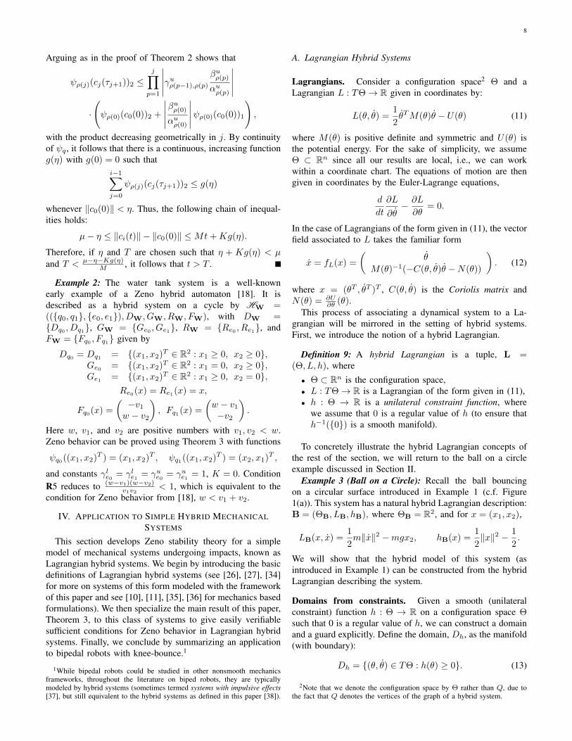
Lagrangians. Consider a configuration space2 Θ and aLagrangian L : TΘ→ R given in coordinates by:

L(θ, θ) =1

2θTM(θ)θ − U(θ) (11)

where M(θ) is positive definite and symmetric and U(θ) isthe potential energy. For the sake of simplicity, we assumeΘ ⊂ Rn since all our results are local, i.e., we can workwithin a coordinate chart. The equations of motion are thengiven in coordinates by the Euler-Lagrange equations,

d

dt

∂L

∂θ− ∂L

∂θ= 0.

In the case of Lagrangians of the form given in (11), the vectorfield associated to L takes the familiar form

x = fL(x) =

(θ

M(θ)−1(−C(θ, θ)θ −N(θ))

). (12)

where x = (θT , θT )T , C(θ, θ) is the Coriolis matrix andN(θ) = ∂U

∂θ (θ).This process of associating a dynamical system to a La-

grangian will be mirrored in the setting of hybrid systems.First, we introduce the notion of a hybrid Lagrangian.

Definition 9: A hybrid Lagrangian is a tuple, L =(Θ, L, h), where

• Θ ⊂ Rn is the configuration space,• L : TΘ→ R is a Lagrangian of the form given in (11),• h : Θ → R is a unilateral constraint function, where

we assume that 0 is a regular value of h (to ensure thath−1({0}) is a smooth manifold).

To concretely illustrate the hybrid Lagrangian concepts ofthe rest of the section, we will return to the ball on a circleexample discussed in Section II.

Example 3 (Ball on a Circle): Recall the ball bouncingon a circular surface introduced in Example 1 (c.f. Figure1(a)). This system has a natural hybrid Lagrangian description:B = (ΘB, LB, hB), where ΘB = R2, and for x = (x1, x2),

LB(x, x) =1

2m‖x‖2 −mgx2, hB(x) =

1

2‖x‖2 − 1

2.

We will show that the hybrid model of this system (asintroduced in Example 1) can be constructed from the hybridLagrangian describing the system.

Domains from constraints. Given a smooth (unilateralconstraint) function h : Θ → R on a configuration space Θsuch that 0 is a regular value of h, we can construct a domainand a guard explicitly. Define the domain, Dh, as the manifold(with boundary):

Dh = {(θ, θ) ∈ TΘ : h(θ) ≥ 0}. (13)

2Note that we denote the configuration space by Θ rather than Q, due tothe fact that Q denotes the vertices of the graph of a hybrid system.

9

Similarly, we have an associated guard, Gh, defined as thefollowing submanifold of Dh:

Gh = {(θ, θ) ∈ TΘ : h(θ) = 0 and dh(θ)θ ≤ 0}, (14)

where dh(θ) =(

∂h∂θ1

(θ) · · · ∂h∂θn

(θ)). Note that 0 is a

regular value of h if and only if dh(θ) 6= 0 whenever h(θ) = 0.

Lagrangian Hybrid Systems. Given a hybrid LagrangianL = (Θ, L, h), the Lagrangian hybrid system associated to Lis the hybrid system

HL = (Γ = ({q}, {(q, q)}), DL, GL, RL, FL),

where DL = {Dh}, FL = {fL}, GL = {Gh} and RL ={Rh} with the reset map given by the Newtonian impactequation Rh(θ, θ) = (θ, P (θ, θ)), with

P (θ, θ) = θ − (1 + e)dh(θ)θ

dh(θ)M(θ)−1dh(θ)TM(θ)−1dh(θ)T .

(15)Here 0 ≤ e ≤ 1 is the coefficient of restitution.

Example 4 (Ball on a Circle): From the hybridLagrangian B = (ΘB, LB, hB) we obtain the Lagrangianhybrid system associated to B:

HB = (Γ = ({q}, {(q, q)}), DB, GB, RB, FB)

It can be checked that this hybrid model is the model HB

introduced in Example 1, i.e., DB, GB, RB, FB as given in(2) are obtained through (13), (14), (15) and (12), respectively.

B. Sufficient Conditions for Zeno Behavior in LagrangianHybrid Systems

This subsection presents sufficient conditions for bounded-time Zeno stability of Lagrangian hybrid systems, based onan explicitly constructed Lyapunov-like function. The paper[10] proves a special case of the main result in this section,Theorem 4, for a class of Lagrangian hybrid systems with con-figuration manifolds of dimension two. If the potential energyis a convex function and the domain specified by the unilateralconstraint is a convex set, global Zeno stability results havebeen proved in [11]. Of course, the convexity assumptionspreclude local phenomena, in which some executions are Zenowhile others are not, occurring in the bouncing ball exampleabove or knee-bounce example below.

First, however, we examine the Zeno equilibria of La-grangian hybrid systems, observing that isolated Zeno equilib-ria only occur in systems with one-dimensional configurationmanifolds. Thus, no Lagrangian hybrid system with configura-tion manifold of dimension greater than one can have bounded-time asymptotically stable Zeno equilibria.

Zeno equilibria in Lagrangian hybrid systems. If HL isa Lagrangian hybrid system, then applying the definition ofZeno equilibria and examining the special form of the resetmaps shows that z = {(θ∗, θ∗)} is a Zeno equilibrium if andonly if

fL(θ∗, θ∗) 6= 0, h(θ∗) = 0,

dh(θ∗)θ∗ ≤ 0, θ∗ = P (θ∗, θ∗).

Furthermore, the form of P implies that θ∗ = P (θ∗, θ∗) holdsif and only if dh(θ∗)θ∗ = 0. Therefore the set of all Zenoequilibria for a Lagrangian hybrid system is given by thesurfaces in TΘ:

Zh = {(θ, θ) ∈ TΘ : fL(θ, θ) 6= 0, h(θ) = 0, dh(θ)θ = 0}.

Note that if dim(Θ) > 1, the Lagrangian hybrid system hasno isolated Zeno equilibria.

Theorem 4: Let HL be a Lagrangian hybrid system and(θ∗, θ∗) ∈ Dh. If the coefficient of restitution satisfies 0 <e < 1 and (θ∗, θ∗) satisfies

h(θ∗) = 0, h(θ∗, θ∗) = 0, h(θ∗, θ∗) < 0,

then {(θ∗, θ∗)} is a bounded-time stable Zeno equilibrium.Here h(θ∗, θ∗) = dh(θ∗)θ∗ and

h(θ∗, θ∗) = (θ∗)TH(h(θ∗))θ∗ +

dh(θ∗)M(θ∗)−1(−C(θ∗, θ∗)θ∗ −N(θ∗)),

where H(h(θ∗)) is the Hessian of h at θ∗.

Proof: First note that {(θ∗, θ∗)} is a Zeno equilibrium.Indeed, dh(θ∗, θ∗)fL(θ∗, θ∗) = h(θ∗, θ∗) 6= 0 implies thatfL(θ∗, θ∗) 6= 0. Then the conditions h(θ∗) = 0 andh(θ∗, θ∗) = 0 imply that {(θ∗, θ∗)} is a Zeno equilibrium.

Let V be a small neighborhood of (θ∗, θ∗) and assume (bypassing to a coordinate chart) that V ⊂ R2n with Euclideannorm. Let K satisfy

K >1 + e

2

‖M(θ∗)−1dh(θ∗)T ‖dh(θ∗)M(θ∗)−1dh(θ∗)T

.

We verify that the constants γuh = γlh = e, K and the function

ψh(θ, θ) =

h(θ, θ) +√h(θ, θ)2 + 2h(θ)

−h(θ, θ) +√h(θ, θ)2 + 2h(θ)

(16)

satisfy conditions R1-R6 on V .R1: Since (θ∗, θ∗) is a Zeno equilibrium, h(θ∗) = 0 and

h(θ∗, θ∗) = dh(θ∗)θ∗ = 0. Thus ψh(θ∗, θ∗) = 0.R2: Since h(θ) ≥ 0, ψh(θ, θ)1 = 0 if and only if h(θ) = 0

and h(θ, θ) ≤ 0. So ψh(θ, θ)1 = 0 if and only if (θ, θ) ∈ Gh.R3: The square root in the definition of ψh creates some

differentiability problems at the Zeno equilibrium.Assume V is small enough that V contains no equilibria of

fL. Then (Dh \ Zh) ∩ V has the form

(Dh \ Zh) ∩ V = {(θ, θ) ∈ V : h(θ) > 0 or h(θ, θ) 6= 0},

and that ψh is continuously differentiable on (Dh \ Zh) ∩ Vwith Lie derivative given by

ψh(θ, θ) =

h(θ, θ) + h(θ,θ)√h(θ,θ)2+2h(θ)

(h(θ, θ) + 1

)−h(θ, θ) + h(θ,θ)√

h(θ,θ)2+2h(θ)

(h(θ, θ) + 1

) .

(17)Recall that h(θ∗, θ∗) < 0. It follows from the definitions

that scaling h by a positive constant does not change Dh, Ghor Rh. Therefore we can assume that h(θ∗, θ∗) = −1.

10

While the function h(θ,θ)√h(θ,θ)2+2h(θ)

may not have a unique

limit as (θ, θ)→ (θ∗, θ∗) it remains bounded on (Dh\Zh)∩V :

|h(θ, θ)|√h(θ, θ)2 + 2h(θ)

≤ 1.

Therefore, ψh has the well defined limit

lim(θ,θ)∈(Dh\Zh)∩V, (θ,θ)→(θ∗,θ∗)

ψh(θ, θ) =

(−11

). (18)

Since the differentiability problems only arise on the guard,an in particular only on the Zeno equilibria, the limit inequation (18) suffices for the evaluation in R3.

R4: Let (θ, θ) ∈ Gh. Then h(θ) = 0 and h(θ, θ) ≤0. So substitution into equation (16) gives ψh(θ, θ) =(0, 2|h(θ, θ)|)T .

Multiplying both sides of equation (15) on the left by dh(θ)and the definition of h(θ, θ) gives h(Rh(θ, θ)) = −eh(θ, θ).

Therefore ψh(Rh(θ, θ)) = (2e|h(θ, θ)|, 0)T . So ifγlh = γuh = e, R4 holds with ψh(Rh(θ, θ))1 ∈[eψh(θ, θ)2, eψh(θ, θ)2].

R5:∣∣∣γuh dψh(θ∗,θ∗)2fL(θ∗,θ∗)

dψh(θ∗,θ∗)1fL(θ∗,θ∗)

∣∣∣ =∣∣∣e 1−1

∣∣∣ = e < 1.

R6: Take a point (θ, θ) ∈ Gh ∩V (this is the only step thatrequires a norm, and hence the coordinate chart on V ). Weupper bound the growth due to the reset map as follows,

‖Rh(θ, θ)− (θ∗, θ∗)‖=

∥∥∥(θ, θ)− (θ∗, θ∗)−(0, (1 + e)

dh(θ)θ

dh(θ)M(θ)−1dh(θ)TM(θ)−1dh(θ)T

)∥∥∥∥∥≤ ‖(θ, θ)− (θ∗, θ∗)‖+

(1 + e)|dh(θ)θ|

dh(θ)M(θ)−1dh(θ)T‖M(θ)−1dh(θ)T ‖.

Recall that ψh(θ, θ)2 = 2|dh(θ)θ|. Plugging in the definitionof K proves R6:

‖Rh(θ, θ)− (θ∗, θ∗)‖ ≤ ‖(θ, θ)− (θ∗, θ∗)‖+Kψh(θ, θ)2.

Since R1-R6 hold, Theorem 3 implies that there is aneighborhood W of (θ∗, θ∗) with W ⊂ V such that thereis a unique Zeno execution with c0(0) = x for all x ∈W .

Example 5 (Ball on a Circle): With Zeno stability toolsin hand, we revisit the ball bouncing on a circle from Examples1, 3 and 4. The conditions in equation (3) for Zeno stabilityfollow from the application of Theorem 4.

C. Application to Knee-bounce in Bipedal Robotic Walking

Mechanical knees are an important component of achievingnatural and “human-like” walking in bipedal robots [39].Mechanical “knee-caps”, i.e., mechanical stops, are typicallyadded to these mechanical knees to prevent the leg from hyper-extending. Yet with this benefit comes a cost: knee-bounce,

z

m

M

mc

mt

mc

mt

y

(a)

Knee-Bounce

se

ze

pep z

Knee-Bounce

se

(b)

Knee-Bounce

se

ze

pep z

Knee-Bounce

se

(c)

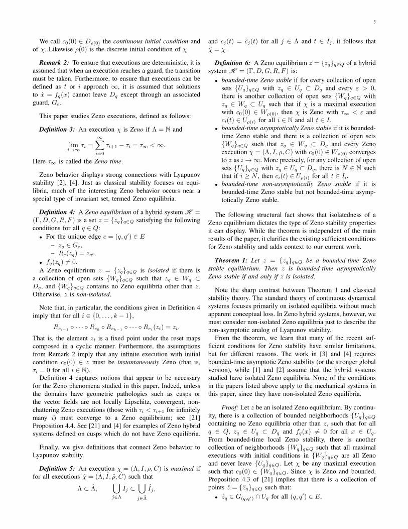
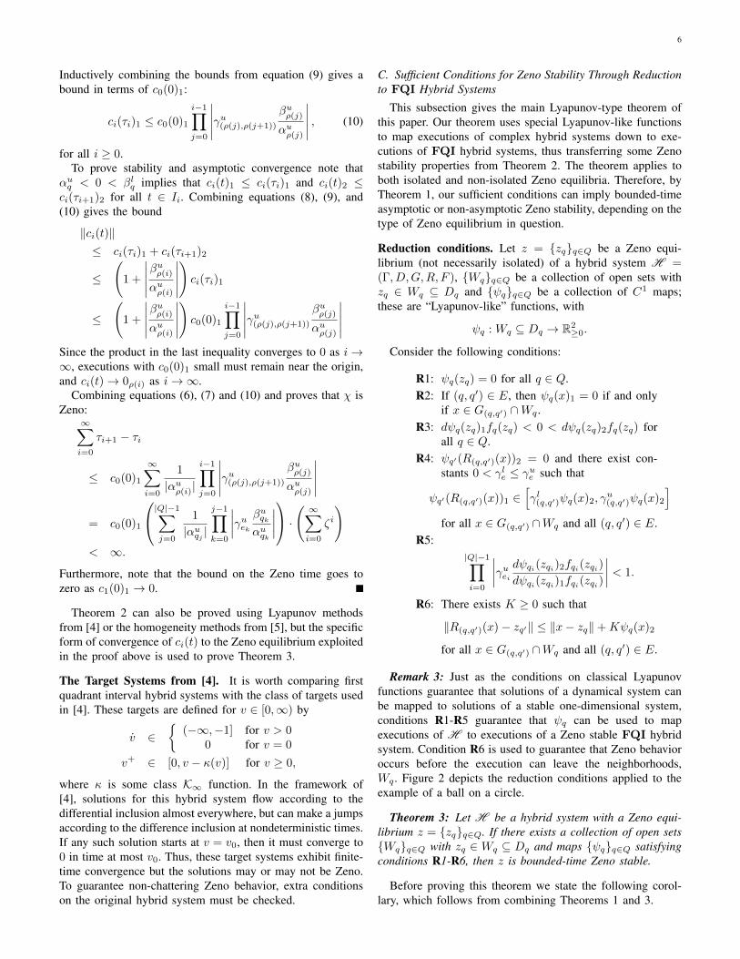
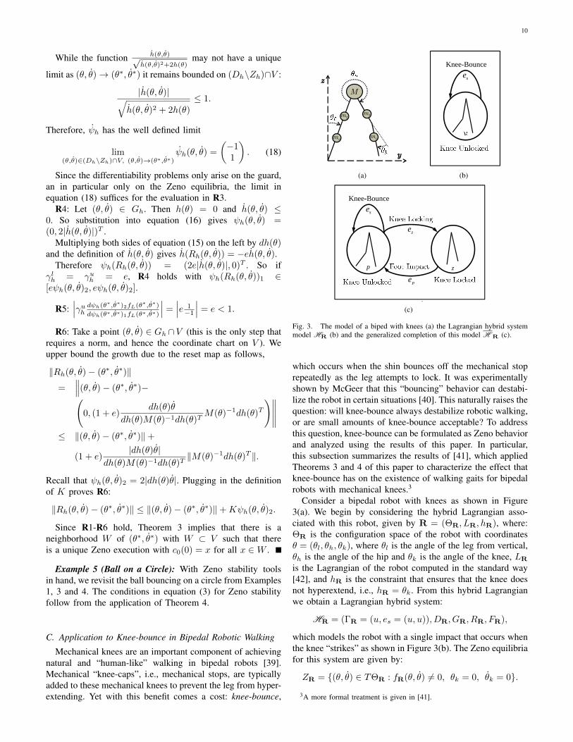
Fig. 3. The model of a biped with knees (a) the Lagrangian hybrid systemmodel HR (b) and the generalized completion of this model H R (c).

which occurs when the shin bounces off the mechanical stoprepeatedly as the leg attempts to lock. It was experimentallyshown by McGeer that this “bouncing” behavior can destabi-lize the robot in certain situations [40]. This naturally raises thequestion: will knee-bounce always destabilize robotic walking,or are small amounts of knee-bounce acceptable? To addressthis question, knee-bounce can be formulated as Zeno behaviorand analyzed using the results of this paper. In particular,this subsection summarizes the results of [41], which appliedTheorems 3 and 4 of this paper to characterize the effect thatknee-bounce has on the existence of walking gaits for bipedalrobots with mechanical knees.3

Consider a bipedal robot with knees as shown in Figure3(a). We begin by considering the hybrid Lagrangian asso-ciated with this robot, given by R = (ΘR, LR, hR), where:ΘR is the configuration space of the robot with coordinatesθ = (θl, θh, θk), where θl is the angle of the leg from vertical,θh is the angle of the hip and θk is the angle of the knee, LR

is the Lagrangian of the robot computed in the standard way[42], and hR is the constraint that ensures that the knee doesnot hyperextend, i.e., hR = θk. From this hybrid Lagrangianwe obtain a Lagrangian hybrid system:

HR = (ΓR = (u, es = (u, u)), DR, GR, RR, FR),

which models the robot with a single impact that occurs whenthe knee “strikes” as shown in Figure 3(b). The Zeno equilibriafor this system are given by:

ZR = {(θ, θ) ∈ TΘR : fR(θ, θ) 6= 0, θk = 0, θk = 0}.

3A more formal treatment is given in [41].

11

That is, the set of points where the knee angle is zero withzero velocity, i.e., the set of points where the leg is straightand the knee is “locked.” Moreover, it is easy to verify thathR < 0 for a large subset of this set, and thus there arestable Zeno equilibria. Physically, the existence of these stableZeno equilibria imply that knee-bounce will occur (formallyverifying the experimental behavior witnessed by McGeer).

As a result of these stable Zeno equilibria, it is necessary tocomplete the Lagrangian hybrid system model HR to allowfor solutions to continue after knee locking. The details of thiscompletion process for this system can be found in [41], but tosummarize one obtains a new hybrid system H R graphicallyillustrated in Figure 3(c) where a “post-Zeno” domain is addedwhere the leg is locked, transitions to that domain occur whenthe set ZR is reached, and transitions back to the original “pre-Zeno” domain occurs at foot-strike with reset map being thestandard impact equations considered in the bipedal roboticsliterature [37]. In the case of perfectly plastic impacts at theknee (when e = 0 for RR as computed with (15)), thiscompleted model is the standard model of a bipedal robotwith knees that lock [43]. What is of interest is when theassumption of perfectly plastic impacts at the knee is relaxed,and knee-bounce occurs.

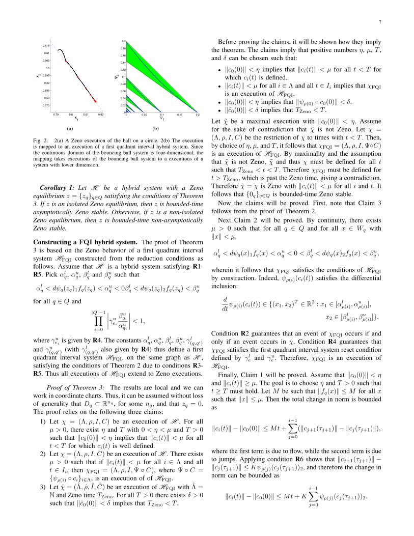
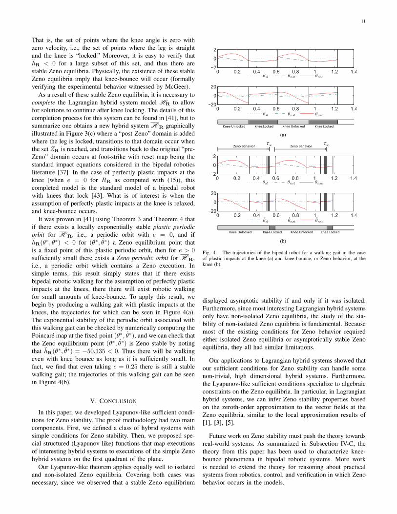
It was proven in [41] using Theorem 3 and Theorem 4 thatif there exists a locally exponentially stable plastic periodicorbit for H R, i.e., a periodic orbit with e = 0, and ifhR(θ∗, θ∗) < 0 for (θ∗, θ∗) a Zeno equilibrium point thatis a fixed point of this plastic periodic orbit, then for e > 0sufficiently small there exists a Zeno periodic orbit for H R,i.e., a periodic orbit which contains a Zeno execution. Insimple terms, this result simply states that if there existsbipedal robotic walking for the assumption of perfectly plasticimpacts at the knees, there there will exist robotic walkingfor small amounts of knee-bounce. To apply this result, webegin by producing a walking gait with plastic impacts at theknees, the trajectories for which can be seen in Figure 4(a).The exponential stability of the periodic orbit associated withthis walking gait can be checked by numerically computing thePoincare map at the fixed point (θ∗, θ∗), and we can check thatthe Zeno equilibrium point (θ∗, θ∗) is Zeno stable by notingthat hR(θ∗, θ∗) = −50.135 < 0. Thus there will be walkingeven with knee bounce as long as it is sufficiently small. Infact, we find that even taking e = 0.25 there is still a stablewalking gait; the trajectories of this walking gait can be seenin Figure 4(b).

V. CONCLUSION

In this paper, we developed Lyapunov-like sufficient condi-tions for Zeno stability. The proof methodology had two maincomponents. First, we defined a class of hybrid systems withsimple conditions for Zeno stability. Then, we proposed spe-cial structured (Lyapunov-like) functions that map executionsof interesting hybrid systems to executions of the simple Zenohybrid systems on the first quadrant of the plane.

Our Lyapunov-like theorem applies equally well to isolatedand non-isolated Zeno equilibria. Covering both cases wasnecessary, since we observed that a stable Zeno equilibrium

0 0.2 0.4 0.6 0.8 1 1.2 1.4−2

0

2

θsl θnst θnsc

0 0.2 0.4 0.6 0.8 1 1.2 1.4−20

0

20

θsl θnst θnsc

Knee Locked Knee Unlocked Knee LockedKnee Unlocked

(a)

0 0.2 0.4 0.6 0.8 1 1.2 1.4−2

0

2

θsl θnst θnsc

0 0.2 0.4 0.6 0.8 1 1.2 1.4−20

0

20

θsl θnst θnsc

Knee Locked Knee Unlocked Knee LockedKnee Unlocked

Zeno Behavior Zeno Behavior

(b)

Fig. 4. The trajectories of the bipedal robot for a walking gait in the caseof plastic impacts at the knee (a) and knee-bounce, or Zeno behavior, at theknee (b).

displayed asymptotic stability if and only if it was isolated.Furthermore, since most interesting Lagrangian hybrid systemsonly have non-isolated Zeno equilibria, the study of the sta-bility of non-isolated Zeno equilibria is fundamental. Becausemost of the existing conditions for Zeno behavior requiredeither isolated Zeno equilibria or asymptotically stable Zenoequilibria, they all had similar limitations.

Our applications to Lagrangian hybrid systems showed thatour sufficient conditions for Zeno stability can handle somenon-trivial, high dimensional hybrid systems. Furthermore,the Lyapunov-like sufficient conditions specialize to algebraicconstraints on the Zeno equilibria. In particular, in Lagrangianhybrid systems, we can infer Zeno stability properties basedon the zeroth-order approximation to the vector fields at theZeno equilibria, similar to the local approximation results of[1], [3], [5].

Future work on Zeno stability must push the theory towardsreal-world systems. As summarized in Subsection IV-C, thetheory from this paper has been used to characterize knee-bounce phenomena in bipedal robotic systems. More workis needed to extend the theory for reasoning about practicalsystems from robotics, control, and verification in which Zenobehavior occurs in the models.

12

REFERENCES

[1] A. D. Ames, A. Abate, and S. Sastry, “Sufficient conditions for theexistence of Zeno behavior in nonlinear hybrid systems via constantapproximations,” in IEEE Conference on Decision and Control, 2007.

[2] A. Lamperski and A. D. Ames, “Lyapunov-like conditions for theexistence of Zeno behavior in hybrid and Lagrangian hybrid systems,”in IEEE Conference on Decision and Control, 2007.

[3] R. Goebel and A. R. Teel, “Zeno behavior in homogeneous hybridsystems,” in IEEE Conference on Decision and Control, 2008.

[4] ——, “Lyapnuov characterization of Zeno behavior in hybrid systems,”in IEEE Conference on Decision and Control, 2008.

[5] ——, “Preasymptotic stability and homogeneous approximations ofhybrid dynamical systems,” SIAM Review, vol. 52, no. 1, pp. 87–109,2010.

[6] A. T. Fuller, “Relay control systems optimized for various performancecriteria,” in IFAC World Congress, 1960.

[7] V. F. Borisov, “Fuller’s phenomenon: Review,” Journal of MathematicalSciences, vol. 100, no. 4, 2000.

[8] V. Acary and B. Brogliato, Numerical Methods for Nonsmooth Dynam-ical Systems: Applications in Mechanics and Electronics. Springer,2008.

[9] J. J. Moreau, Unilateral Contact and Dry Friction in Finite FreedomDynamics. Springer-Verlag, 1988, pp. 1–82.

[10] Y. Wang, “Dynamic modeling and stability analysis of mechanicalsystems with time-varying topologies,” Journal of Mechanical Design,vol. 115, pp. 808–816, 1993.

[11] A. Cabot and L. Paoli, “Asymptotics for some vibro-impact problemswith a linear dissipation term,” Journal de Mathmatiques Pures etAppliqus, vol. 87, no. 3, pp. 291 – 323, 2007.

[12] M. K. Camlibel and J. M. Schumacher, “On the Zeno behavior of linearcomplementarity systems,” in 40th IEEE Conference on Decision andControl, 2001.

[13] J. Shen and J.-S. Pang, “Linear complementarity systems: Zeno states,”SIAM Journal on Control and Optimization, vol. 44, no. 3, pp. 1040–1066, 2005.

[14] D. L. Dill, “Timing assumptions and verification of finite-state con-current systems,” in Automatic Verification Methods for Finite StateSystems. Springer, 1990.

[15] A. Nerode and W. Kohn, Models for Hybrid Systems: Automata,Topologies, Controllability, Observability. Springer-Verlag, 1993.

[16] R. Alur, C. Courcoubetis, N. Halbwachs, T. A. Henzinger, P.-H. Ho,X. Nicollin, A. Olivero, J. Sifakis, and S. Yovine, “The algorithmicanalysis of hybrid systems,” Theoretical Computer Science, vol. 138,no. 1, pp. 3–34, 1995.

[17] K. H. Johansson, J. Lygeros, S. Sastry, and M. Egerstedt, “Simulationof Zeno hybrid automata,” in Proceedings of the 38th IEEE Conferenceon Decision and Control, Phoenix, AZ, 1999.

[18] J. Zhang, K. H. Johansson, J. Lygeros, and S. Sastry, “Zeno hybridsystems,” Int. J. Robust and Nonlinear Control, vol. 11, no. 2, pp. 435–451, 2001.

[19] M. Heymann, F. Lin, G. Meyer, and S. Resmerita, “Analysis of Zenobehaviors in a class of hybrid systems,” IEEE Transactions on AutomaticControl, vol. 50, no. 3, pp. 376–384, 2005.

[20] A. D. Ames, A. Abate, and S. Sastry, “Sufficient conditions for theexistence of Zeno behavior,” in 44th IEEE Conference on Decision andControl and European Control Conference, Seville, Spain, 2005.

[21] S. Simic, K. H. Johansson, S. Sastry, and J. Lygeros, “Towards ageometric theory of hybrid systems,” Dyanmics of Discrete, Continuous,and Impulsive Systems, Series B, vol. 12, no. 5-6, pp. 649–687, 2005.

[22] R. Goebel and A. R. Teel, “Solutions to hybrid inclusions via set andgraphical convergence with stability theory applications,” Automatica,vol. 42, pp. 573–587, 2006.

[23] A. D. Ames, P. Tabuada, and S. Sastry, “On the stability of Zenoequilibria,” in Hybrid Systems: Computation and Control, ser. LectureNotes in Computer Science, J. Hespanha and A. Tiwari, Eds., vol. 3927.Springer-Verlag, 2006, pp. 34–48.

[24] A. Lamperski and A. D. Ames, “On the existence of Zeno behavior inhybrid systems with non-isolated Zeno equilibra,” in IEEE Conferenceon Decision and Control, 2008.

[25] Y. Or and A. D. Ames, “Stability of Zeno equilibria in Lagrangian hybridsystems,” in IEEE Conference on Decision and Control, 2008.

[26] ——, “Formal and practical completion of Lagrangian hybrid systems,”in ASME/IEEE American Control Conference, 2009.

[27] ——, “Existence of periodic orbits with Zeno behavior in completedLagrangian hybrid systems,” in Hybrid Systems: Computation andControl, 2009.

[28] Y. Or and A. R. Teel, “Zeno stability of the set-valued bouncing ball,”IEEE Transactions on Automatic Control, vol. 56, pp. 447–452, 2011.

[29] Y. Or and A. D. Ames, “Stability and completion of zeno equilibria inlagrangian hybrid systems,” IEEE Transactions on Automatic Control,vol. 56, pp. 1322–1336, 2011.

[30] J. M. Schumacher, “Time-scaling symmetry and Zeno solutions,” Auto-matica, vol. 45, no. 5, pp. 1237–1242, 2009.

[31] H. K. Khalil, Nonlinear Systems, 2nd ed. Prentice Hall, 1996.[32] J. P. Aubin and H. Frankowski, Set Valued Analysis. Birkhauser, 1990.[33] A. Filippov, Differential equations with discontinuous right-hand sides.

Kluwer Academic Publishers, 1988.[34] A. D. Ames and S. Sastry, “Routhian reduction of hybrid Lagrangians

and Lagrangian hybrid systems,” in American Control Conference, 2006.[35] P. Ballard, “The dynamics of discrete mechanical systems with perfect

unilateral constraints,” Archive for Rational Mechanics and Analysis,vol. 154, pp. 199–274, 2000.

[36] B. Brogliato, Nonsmooth Mechanics. Springer-Verlag, 1999.[37] E. R. Westervelt, J. W. Grizzle, C. Chevallereau, J. H. Choi, and

B. Morris, Feedback Control of Dynamic Bipedal Robot Locomotion.Taylor & Francis, 2007.

[38] J. W. Grizzle, C. Chevallereau, A. D. Ames, and R. W. Sinnet, “3Dbipedal robotic walking: models, feedback control, and open problems,”in IFAC Symposium on Nonlinear Control Systems, Bologna, 2010.

[39] T. McGeer, “Passive walking with knees,” in IEEE International Con-ference on Robotics and Automation, 1990.

[40] “Experimentally observed knee-bounce in bipedal robotic walking,”http://www.youtube.com/watch?v=qYWiC3J7GK8.

[41] A. D. Ames, “Characterizing knee-bounce in bipedal robotic walking: Azeno behavior approach,” in Hybrid Systems: Computation and Control,Chicago, IL, 2011.

[42] R. M. Murray, Z. Li, and S. S. Sastry, A Mathematical Introduction toRobotic Manipulation. Boca Raton: CRC, mar 1994.

[43] A. D. Ames, R. Sinnet, and E. Wendel, “Three-dimensional kneedbipedal walking: A hybrid geometric approach,” in Hybrid Systems:Computation and Control, ser. Lecture Notes in Computer Science,R. Majumdar and P. Tabuada, Eds. Springer Berlin / Heidelberg, 2009,vol. 5469, pp. 16–30.

Andrew Lamperski (S’05–M’12) is a postdoctoralscholar in control and dynamical systems at the Cal-ifornia Institute of Technology, where he obtaineda Ph.D. degree in 2011. In 2004, he obtained aB.S. degree from The Johns Hopkins Universityin biomedical engineering and mathematics. Hisinterests are in decentralized control, hybrid systems,and neuroscience applications.

Aaron D. Ames is an Assistant Professor in Me-chanical Engineering at Texas A&M University, witha joint appointment in Electrical and Computer En-gineering. His research interests center on robotics,nonlinear control and hybrid systems, with specialemphasis on bipedal robots, behavior unique tohybrid systems such as Zeno behavior, and the math-ematical foundations of hybrid systems. Dr. Amesreceived a BS in Mechanical Engineering and a BAin Mathematics from the University of St. Thomasin 2001, and he received a MA in Mathematics and

a PhD in Electrical Engineering and Computer Sciences from UC Berkeleyin 2006. At UC Berkeley, he was the recipient of the 2005 Leon O. ChuaAward for achievement in nonlinear science and the 2006 Bernard FriedmanMemorial Prize in Applied Mathematics. Dr. Ames served as a PostdoctoralScholar in the Control and Dynamical System Department at the CaliforniaInstitute of Technology from 2006 to 2008. In 2010 he received the NSFCAREER award for his research on bipedal robotic walking.