Lund UniversityCentre for Mathematical Sciences Mathematical Statistics

Master’s ThesisSeptember 25, 2015

On Climate Change and Its Impact on Extreme Rainfall in Bangladesh

Nasrin Sultana

Supervisor : Nader Tajvidi

1

AbstractIn recent years extreme value distributions have attracted a fair amount of attention in literaturefor risk assessment based on climate data. This thesis focuses on modeling a series of rainfall data over 58 years in the period 1954-2012 recorded at five different stations in Bangladesh. Inference on the extreme rainfall is essential for making the necessary steps to reduce damage caused by natural calamities as well as to save life and property. One might ask if extreme rainfalls are occurring more frequently now or whether there is dependence in extreme rainfalls between two regions. To answer these questions, considering a bivariate framework, we model rainfall data from two stations simultaneously and investigate the dependence structure in extreme rainfall between the locations. As a starting point the generalized extreme value distributions are used for fitting annual maximum rainfall according to the Block Maxima approach. Also generalized Pareto distributions are fitted to daily rainfall data considering Peaks over Thresholds (PoT) method. We assess the uncertainty in the estimates of the parameters by constructing 95% confidence interval using both delta and profile likelihood methods. Return levels for different return periods are also estimated for both models. Monte Carlo simulation approach is suitable to predict future return level when the number of exceedances is uncertain. Thereafter, return levels with bootstrap confidence interval are estimated from simulated data. Finally, we model the tail dependence of extreme rainfall between two locations using bivariate extreme value distribution (BEVD) and bivariate generalized Pareto distribution (BGPD) with unit Fréchet margins. In recent years this extreme value distributions have attracted a fair amount of attention in literature for risk assessment based on climate data. Both parametric and non-parametric dependence functions are used in BEVD models. In addition, BGPD models are fitted considering 95% thresholds based on daily rainfall data but only parametric dependence structure are considered in this case. Finally we quantify risks by calculating joint probability of extreme rainfalls using BEVD models.

Key words: generalized extreme value distribution, generalized Pareto distribution, return level, bivariate extreme value distribution, bivariate generalized Pareto distribution, climate change,dependence.

.

2

AcknowledgementsFirst, I would like to thank and express my deepest gratitude to my supervisor, Nader Tajvidi at the Faculty of Engineering Lund University for giving me the opportunity under his excellent guidance, patience and for bringing my attention to the field of extreme value theory. His outstanding teaching in the courses “Statistical Modeling of Extreme Values” and “Statistical Modeling of Multivariate Extremes” encouraged me to work in this area.

I would also like to thank Magnus Wiktorsson for offering me the opportunity to study at Lund University. I am really grateful for his continuous support and suggestions whenever I looked for as my director and coordinator in the last two years.

I would like also to thank Mr. Rezaul Roni, Assistant Professor, Department of Geography and Environment at Jahangirnagar University, Bangladesh for his nice helping attitude and collecting the data from Bangladesh Meteorological Department in favor of me. Therefore I wish to acknowledge Bangladesh Meteorological Department for this assistance.

Finally, I would like to thank Almighty Allah for giving me such a lovely girl. I would never have been able to finish my MS without her unbounded patience. Last but not least thanks to my dear husband for his continuous encouragement and nice cooperation.

3

Contents

1. Introduction ……………………………….…………………………..……………………………...51.1. Impact of Climate Change in Bangladesh…………………………………………………… 5-71.2. Background of Extreme value Analysis…………………………………………………………..7

2. Extreme Value Modeling…………………..………………………………………………………...9

2.1. Generalized Extreme Value Distribution ………………………………………………………..92.1.1.Basic concept of GEV……………………………………………………………………….92.1.2.Return Level………………………………………………………………………………..11

2.2. Inference for Generalized Extreme Value Distribution ………………………….......................122.2.1.MLE of Parameters and Confidence Interval…………………………………....................122.2.2.MLE of Return Levels and Confidence Interval………………………………...................12

2.3. Asymptotic Model for Minima……………………………………………………………….....132.4. Generalized Pareto Distribution…………………………………………………………………13

2.4.1.Basic concept of GPD……………………………………………………………………...132.4.2.Threshold Selection………………………………………………………………………...142.4.3.Return Levels………………………………………………………………………………14

2.5. Inference for Generalized Pareto Distribution…………………………………………………..152.6. Connection with Poisson Distribution: Poisson-GPD Model for Exceedances…………………152.7. Extremal Index :Measure of Stationarity………………………………………………………..162.8. Model Validation……………………………………………………………………………......16

2.8.1. quantile – quantile(q-q) Plot ………………………………………………………………162.8.2.Goodness of Fit Test……………………………………………………………………….172.8.3.Likelihood Ratio Test………………………………………………………………………17

3. Multivariate Extreme……………………………………………………………………………….18

3.1. Dependence Measure……………………………………………………………………………183.1.1.Pearson’s rho……………………………………………………………………………….183.1.2.Kendall tau……………………………………………………………………………........18

3.2. Max Stable and Max-infinite Divisibility……………………………………………………….193.3. Component Wise Maxima………………………………………………………………………213.4. Density Function of BEVD……………………………………………………………………...223.5. Measures of Extreme Dependence…………………………………………………………........23

3.5.1.Parametric Models………………………………………………………………………....233.5.2.Non-Parametric Models………………………………………………………………........23

3.6. Multivariate Generalized Pareto Distribution…………………………………………..............253.7. Density Function of BGPD……………………………………………………………………...26

4. Data and Rainfall Pattern of Studied Stations………………………………………………….....28

4.1. Data……………………………………………………………………………………………...284.2. Overview of Rainfall ……………………………………………………………………………28

4.2.1.Station Barisal……………………………………………………………………………...284.2.2.Station Khulna…………………………………………………………………………….. 294.2.3.Station Satkhira…………………………………………………………………………….294.2.4.Station Bogra…………………………………………………………………………….....294.2.5.Station Rangpur………………………………………………………………………….....29

4

4.3. Empirical Upper Quantile ………………………………………………………………………30

5. Analysis of Rainfall………………………………………………………………………………….31

5.1. Method of Finding Suitable Models…………………………………………………………….31

Part A : Univariate Extreme Value Modeling

5.2. Univariate Extreme Value Analysis……………………………………………………………..325.2.1.Stationarity and Trend Checking…………………………………………………………..325.2.2.Threshold Selection for GPD……………………………………………………………....335.2.3.Model Checking Plots………………………………………………………………….......335.2.4.Parameters Estimation……………………………………………………………………...335.2.5.Return Levels of Rainfall…………………………………………………………………..35

5.3. Prediction of Maximum Future Rainfall Using MCMC……………………………………..37-38

Part B : Bivariate Extreme Value Analysis

5.4. Correlation Pattern Between Stations…………………………………………………………...395.5. Component Wise Maxima :Modeling BEVD………………………………………………. …405.6. Bivariate Peaks Over Threshold Models……………………………………………………. …425.7. Probability of Extreme Rainfall Estimation…………………………………………………….44

6. Result Discussion and Conclusion ……………………………………………………………........46

6.1. Discussion of results………………………………………………………………………….....466.2. Further Scope……………………………………………………………………………………47

Appendix: Notation used in this thesis

Plots

References

5

Chapter 1

Introduction1.1 Consequences of Climate Change in Bangladesh

Bangladesh is highly vulnerable to natural disasters because of its geographical location, flat and low-lying landscape. The location of Bangladesh is in monsoon region of South Asia surrounded by the Bay of Bengal and the Indian Ocean to the south and iced-cap Himalayan range to the north that made it one of the wettest countries of the world.[1] Any change of monsoon climate makes it sensitive to different natural disasters like, floods and cyclones.[2]

The Intergovernmental Panel on Climate Change (IPCC) is the top most international body for assessment of climate change and the recent fifth assessment report from Working Groups 2 (‘Impacts, Vulnerability and Adaptation’) explore the major impacts of climate change, the apparent effects of these impacts and the present situation, challenges and future directions for adaptation for Bangladesh, South Asia, the Least Developed Countries and the rest of the world. The climate change can be defined by IPCC as the significant changes on state of climatic that could be identified by variation of the mean and/or variabilities of its properties and continues for a prolonged period, usually decades or longer. The impacts of climate have already observed and over next two decades will become more severe.[3] Climate change is one of the most alarming issue for Bangladesh. According to the World Risk Index 2011(jointly conducted by United Nations University (UNU), Germany and the Institute of Environment and Human Security) Bangladesh ranks sixth on the list of countries which are most susceptible to natural disasters, whereas second among the Asian countries.[2]

There is a notable change in weather pattern and climatic behavior in Bangladesh due to climate change. Almost every year Bangladesh have to face different types of natural disasters due to the global warming as well as Climate Change. According to the fifth assessment report, sea level rise, high temperature, heat waves, cyclones and storm surges, salinity intrusion, heavy rainfall and high humidity are the remarkable anticipated impact due to climate changes. Because of rising sea levels, Bangladesh is vulnerable to increasing salinity of their ground water as well as surface water resources especially along the coast. The Sunderban mangrove forest is likely to be lost as well as some loss of land and people will become home- less. Furthermore, several epidemic diseases such as cholera and diarrhea, outbreak of dengue, causing stress and tension and blood pressure are more likely to increase due to these climate changes.[4] Fourth Assessment Report of IPCC accomplished human made emissions of greenhouse gases can be blamed for the harmful effects of climate change. Fourth Assessment report of IPCC described following changes in climate trends, variability and extreme events occurred in Bangladesh

In Bangladesh, the average temperature has registered an increasing trend of about 1°C in May and 0.5°C in November during the 14 year period from 1985 to 1998.

The annual mean rainfall exhibits increasing trends in Bangladesh. Severe and recurring floods have taken place during 2002, 2003, and 2004.

6

Monsoon depressions frequency and cyclones formation in Bay of Bengal has increased. Saltwater from the Bay of Bengal is reported to have penetrated 100km or more

inland along tributary channels during the dry season. The precipitation decline and droughts has resulted in the drying up of wetlands

and severe degradation of ecosystems.[5]

Studying the impact of climate change is a substantial area and our first consideration is rainfall, one of the substantial indicator of climate change. Then the next concern will be other indicator like temperature, sea-level rise and humidity etc. Bangladesh have experienced the heaviest rainfall in the world for rainfall overwhelmed atmosphere. [6] Among several consequences, one of vital impact of climate change is heavy and unpredictable rainfall. Previously, a good number of research were conducted to find the influential factors that are accountable for extreme rainfall. Researchers found that this increasing intensity and variability of rainfall are the effect of climate change [7] and also Global Climate Models identify the global warming is responsible for increasing intensity of extreme precipitation events.[8] Another study explains the climate changes would reinforce monsoon circulation, increase surface temperature, and increase the magnitude and frequency of extreme rainfall events.[9] The changing behavior of rainfall are definitely consequences the changing climate change [1] as well as the extreme precipitation and changes in sea level are relevant to river and coastal flooding.[10]

Most of the climatic models projected that the increase of rainfall during the monsoon season and decrease in rainfall in the dry season the in south Asian region.[11] According to the Intergovernmental Panel on Climate Change (IPCC) special report on the regional impacts of Climate Change [5], Bangladesh will get about 5% to 6% increase of rainfall by 2030 for glacier melting and more intense monsoons. The increased rainfall follows the risk of more recurrent and severe floods; the southern region will face more coastal flooding and saline interruption. At the same time the drier northern and western parts might suffer from more prolonged droughts. [7, 8] Regular river floods affect 20% of the country, increasing up to 68% in extreme years. The Bangladesh National Plan for Disaster Management 2010-2015 distinguishes four different types of floods such as flash floods caused by overflowing of hilly rivers of eastern and northern Bangladesh, rain floods caused by drainage congestion and heavy rains, monsoon floods caused by major rivers usually in the monsoon and coastal floods caused by storm surges and tides.[12]

Bangladesh has already experienced severe floods in 1988, 1998, 2004, and 2007, 2014, 2015; and cyclones and tidal surges in 1991, 1998, 2000, 2004 and 2007, 2015. According to WMO figures, 210 mm of rain fell in Cox’s Bazar and 135 mm in Barisal were recorded in 2015.[13] The excess of rainfall Millions of people in northern Bangladesh are threatened by riverbank erosion homes were reported flattened or flooded and power supplies were disrupted, outbreak of diarrheal diseases and severe food insecurity.[14] International Federation of the Red Cross and Red Crescent Societies in 2000 identified river erosion as the largest concern for Bangladesh.[15]

In agricultural economy based country Bangladesh, around 80% people live in rural area and directly or indirectly depend on agriculture. The unpredictable rainfall and the natural hazards due to excess rainfall may affect ecosystems, productivity of land, agriculture and food security. The extent of climate changes may observed to be small but they could substantially increase the

7

frequency and intensity of existing climatic events (floods, droughts, cyclones etc.). Recent floods and cyclones become more severe and unpredictable or off seasonal. Therefore, it is essential to estimate the exact degree of change and extrapolated rainfall statistically to overcome and adapt these phenomenon. Necessary preparation for oncoming extreme weather events should be taken to avoid these extensive environmental and economic losses including loss of lives.

1.2. Background of Extreme value AnalysisIn weather and climate studies, extreme events are especially interested rather usual events. The extreme events are defined as very high or low frequency of events with a low probability of occurrence. Statistical modeling of extreme values has developed widely during the last decades. The collection of recent books (Coles (2001), Embrechts et al. (1998), Kotz and Nadarajah (2000), Beirlant et al. (2005), and a large journal literature provide us an extensive overview about the theory and application of Extreme value.[16]

Extreme value theory is branch of probability and statistics, used to develop stochastic models to describing the behavior of the extreme observations; especially the extremes of most meteorological variables such as wind speed, precipitation, temperature, wave heights, flood and also risk analysis of financial data like insurance claims, price fluctuations are concerned. Multivariate extreme value distributions developed in linking with extremes of a random sample from a multivariate distribution.[17] The sources/causes of environmental extremes may be different for example at several points of a river or sea port and allowing different sources environmental extreme, modeling dependence structure between extremes has developed.[18] So statistical inference for joint extreme events has been an intensive research to practitioners since rare events can have serious natural and economic impact. It is studying the positive dependent distributions with dependence in the extreme upper tails, with this property known as tail dependence.[19] An ambiguous evaluation of the dependence in the tails of a multivariate distribution may have significant effect in underestimation of risks from crises events.[20]

Thus the main interest is to model extreme rainfall data from Bangladesh and with the help of bivariate extreme modeling approach estimating risk of extreme rainfall. This paper is structured as follows. Chapter 1 gives introduction and the motivation of studying extreme rainfall in perspective of Bangladesh, Chapter 2 briefly introduces Extreme value models and inferences of models Chapter 3 introduces the dependence structure modeling, and the multivariate extreme value theory focusing bivariate case. Chapter 4 Overview of rainfall pattern of the studied stations Chapter 5 carries out empirical work with the corresponding results in the form of tables and figures. Chapter 6 gives discussion of results and further scope of studies.

8

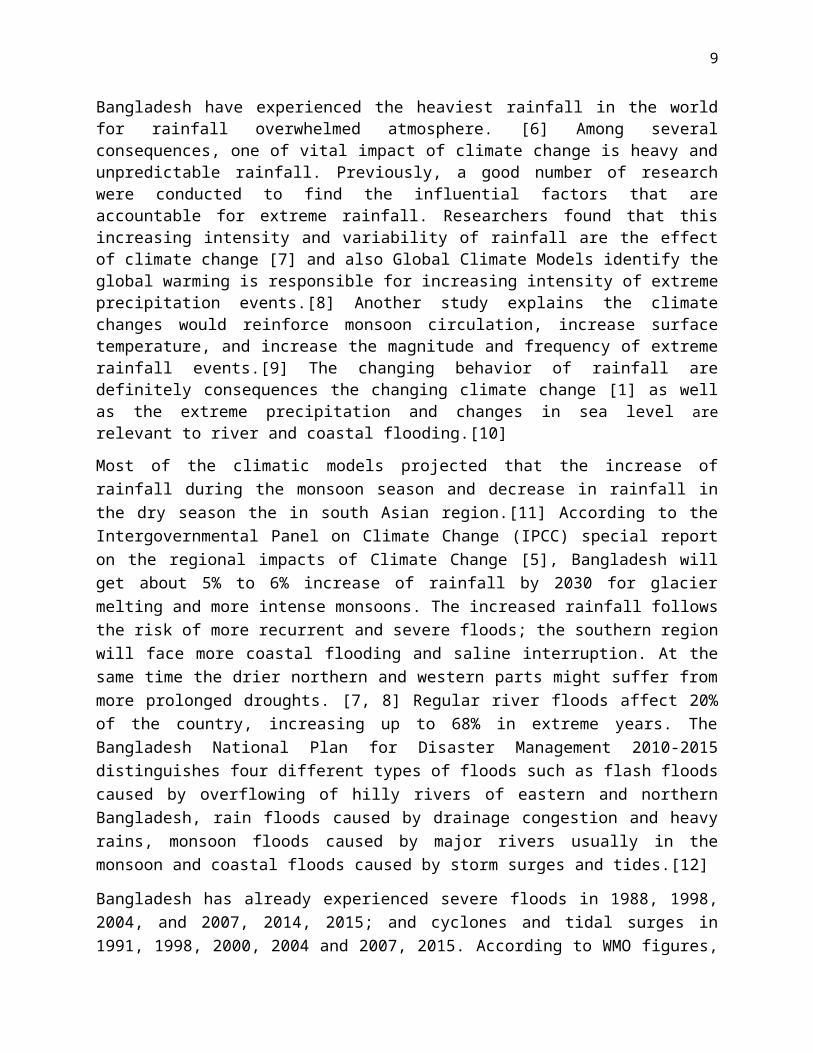
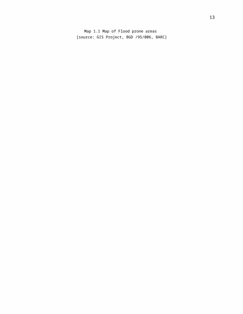
The following map of Bangladesh indicating the different levels of flooding and tidal surges across the country.

Map 1.1 Map of Flood prone areas [source: GIS Project, BGD /95/006, BARC]

Khulna

Satkhira

Rangpur

Bogra

Barisal

9

Chapter 2

Extreme Value ModelingThis chapter is going to outline in brief the parametric modeling of univariate extremes.

2.1 Generalized Extreme Value Distribution

2.1 .1 Basic Concept of GEV

Consider X1 , X2 , X3……………. X nis a sequence of independent and identically distributed random variables, having a common continuous distribution function F and M n represents the maximum value of the process over n∈N time units of observation. In practice, if X1 , ..., X365 is recorded daily maximum rainfall then M n represents the maximum rainfall in a year and can be written as

M n=max (X1 , X2 , X3…………….X n)

The distribution of Mn can be derived for all values n

Pr (M n<x )=P ( X1≤ x ,……X n≤ x )

¿ P ¿

¿ Fn(x)

The distributionFunknown even for some known distribution computation are sometimes much complicated. Therefore, it is convenient to studying the behavior of Fn(x) as n→∞ . For any z<z+¿∧ z+¿ ={F (z )< 1} ¿¿ ¿,F

n(x)→0 as n→∞ so the distribution of M n is degenerate concentrated at a point on z+¿¿. After renormalizing the variable M n in the following form it becomes straightforward and free of computational difficulty.

M n¿<

M n−bn

an

For some constant an >0 and bn ∈ R limiting distributionM n¿ is our main concern.

Theorem 2.1 Suppose normalizing constants an > 0 and bn ∈ R are such that

limn→∞

Pr (M n−bn

an¿≤x )=lim

n→∞Fn (an x+bn )=G ( x )¿

Here G(x) is non-degenerate distribution function. “The external types” theorem refers that the only possible limits for G(x) are given by the following three types of distributions:

Type I (Frechet distribution):G ( x )={ 0 x≤b

exp {−( x−ba )

−α}x>b

10

Type II (Weibull distribution): G ( x )={exp {−[−x−ba ]

α}x<b

1 x≥b

Type III (Gumbel distribution):G ( x )=exp {−exp[−( x−ba )]} , −∞<x<∞

Therefore by Theorem 2.1 for stabilized Mn, the limiting distribution of corresponding M n¿ must

follow one of the three types of extreme value distribution. The result contains contributions by Fisher, Tippet and Gnedenko. The re-parametrization technique by von Mises shows that these three types of distributions can be combined to a one single family of model by changing location and scale. This single distribution popularly known as generalized extreme value (GEV) distribution and can be written as

G ( x ;γ , μ , σ )=exp ¿ ……………….(2.1)

The GEV distribution has three parameters. Location parameter denoted by μ specifies the center of the GEV distribution. Scale parameter, denoted byγ, determines the size of deviations of μ.The shape parameter which denoted by γ shows how rapidly the upper tail decays. The positive γimplies a heavy tail while negative one implies a bounded tail, and the limit of γ→0 implies an exponential tail. These cases correspond to type I (Fréchetdistribution) and type II (Weibulldistribution) distributions respectively. For γ = 0 interpreted as the limit which leads to the double exponential or type III (Gumbel).

Moreover from the notation x+¿=max ( x, 0) ¿ the end point of distributions is

x>µ−σγ for γ > 0

and x<µ−σγ for γ < 0.

The Theorem 2.1 can be restated as follows

Theorem 2.2 If there exist sequences of constants for {an¿0} and bn such that

pr {M n−bn

an≤x }→G(x)

As n→∞, for G is a non-degenerate distribution function and member of the GEV family

defined on {x :1+γx−μσ

>0 } where −∞<μ<∞∧−∞<γ<∞.

The extreme value distribution is used to model the maximum for each block where blocks are partitioned in to non-overlapping periods of equal sizes (say n). Suppose i.i.d. X1 , X2 , X3……………. X nobservations are divided in to m blocks of size n. Then M n ,1 ,……… .., M n ,m are the maximum values from each block. The distributions of these maximum observations can be approximated by the asymptotically motivated GEV distribution. In order to obtain good asymptotic approximation we must not keep block size too small.

11

12

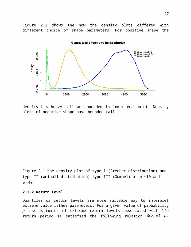
Figure 2.1 shows the how the density plots differed with different choice of shape parameters. For positive shape the density has heavy tail and bounded in lower end point. Density plots of negative shape have bounded tail.

Figure 2.1.the density plot of type I (Fréchet distribution) and type II (Weibull distribution) type III (Gumbel) at μ =10 and σ=40

2.1.2 Return Level

Quantiles or return levels are more suitable way to interpret extreme value rather parameters. For a given value of probability p the estimates of extreme return levels associated with 1/p return period is satisfied the following relation G(z p)=1−p . Inverting the GEV distribution, extreme quantiles can be estimated as follows

z p=¿…………… (2.2)

Therefore any particular block maima exceeds the value z p with probability p and the level z p is expected to be exceded on average once in every 1/p years.

0 1000 2000 3000 4000 5000

0.00

00.

004

0.00

8

Generalized Extreme value distribution

Den

sity

Gamma=0.5Gamma=-0.5Gamma=0

13

2.2Inference for Generalized Extreme Value Distribution

2.2.1 MLE of Parameters

The estimates of unknown parameters of GEV can be obtained by maximizing the log likelihood with respect to parameter vectors (μ ,σ , γ ).The log likelihood of GEV can be written as

l (μ ,σ , γ )={−mlogσ−(1+ 1γ )∑i=1

m

log [1+γ ( x i−μσ )]−∑

i=1

m [1+γ ( x i−μσ )]

−1γfor γ ≠0

−mlogσ−∑i=1

m

( x i−μσ )−∑

i=1

m

exp [−( xi−μσ )] for γ=0

…………..(2.3)

Provided [1+γ ( x i−μσ )]>0 for i=1,2 ,…..m

Otherwisel (μ ,σ , γ )=−∞

The maximization is straightforward using standard numerical optimization algorithm for a given dataset. The approximate distribution of ( μ , σ , γ ) follows multivariate normal distribution with mean (μ , σ , γ ) and variance is the inverse of observed information matrix. The 95% CI of parameters can be estimated using delta and profile likelihood methods.

2.2.2 MLE of Return Levels and CI

The MLE of return levels is obtained by substituting ( μ , σ , γ ) in equation (2.2) and the

z p=¿

95% CI estimated by delta method and profile likelihood methods. By delta method

v ( z p )≈∇ z pTV ∇ z p and V=variance covariance matrix of ( μ , σ , γ )

∇ z pT=[ δ z p

δμ,δ z p

δσ,δ z p

δγ ]¿ [1 , γ−1 (1− y p

−γ ) , σ γ−2 (1− y p−γ )−σ γ−1 y p

−γ log y p ]For γ<0the estimated upper end point that is infinite observation return periods regarding zp with probability p is obtained by

z0= μ− σγ and ∇ z0

T=[1 ,−γ−1, σ γ ¿2 ]

The upper end point for γ=0 is infinite .The poor normal approximation of MLE leads the interpretation of return levels inference for long run return periods sensitive.Better

14

approximation is obtained by profile likelihood method. Delta and profile likelihood method are briefly explain in Appendix

15

2.3Asymptotic Model for Minima

The minimum of data defined as ~M n and let Y i=−X i i=1,2 ,……n and it can be written that ~M n=−M n.then the asymptotic distribution of ~M n also follows GEV with parameters (-μ ,σ , γ ¿.

2.4Generalized Pareto distribution

2.4. Basic Concept of GPD

Generalized Pareto distribution is another way to modeling the statistical behavior of extreme data concerning the data from entire time series .If the entire time series data available this approach would be more informative and efficient than annual maxima. The peaks over threshold technique is usually applied to model daily data and this procedure was promoted by Davison and Smith (1990), however Pickands (1975) was the developed the asymptotic characterization. Assuming the daily data { X1 , X2 , X3 ,……} is independent sequence of with common distribution functionF. Since this approach considering only the values that are exceed the high threshold u then the conditional distribution of excesses of a threshold u is determined by

Pr ( (X>u+x ) /X>u )=1−F (u+x )1−F (u)

, x>0……………………(2.5)

For known distribution (F) refers known threshold distribution. The new distribution generalized Pareto distribution (GPD) is obtained by using GEV as an approximation to this distribution.

Theorem 2.3 Let {X1 , X2 , X3 ,……} be a sequence of random variable with distribution function F and Mn is defined as M n=Max {X1 , X2 , X3 ,…… }.For an arbitrary term X from the sequence X i and F satisfies the theorem 2.2 so that for large n

Pr (M n<z )≈G(z)

Where G(z )=exp {−[1+γ ( z−μσ )]

−1γ } for μ∧σ>0 and γ

For large value of uthe distribution function of (X−u), conditional on x>u approximately follows

H ( x )={ 1−(1+γ x~σ )

−1γ for γ ≠0

1−exp(−x~σ )

−1γ for γ=0

………………(2.6)

Defined on {x : x>0∧(1+γ x~σ )>0} where ~σ=σ+γ (u−μ )

16

The family of distribution defined by equation 2.6 known as generalized Pareto distribution family .The above theorem 2.3 provide link between GEV and GPD. The parameters GPD fit are uniquely determined by associated with GEV of block maxima. The qualitative behavior of GPD depends on shape (γ) ,for example , γ<0 refers the bounded distribution and , γ>0 indicate no upper bound and , γ=0 refers unbounded distribution.

2.4.2 Threshold Selection

The threshold selection process is likely to selection of block by implying a trade of between bias and variance. Too low threshold have possibility to disrupt the asymptotic bias of the model and too high threshold leading the estimated model to a high variance. There are two methods have been used to select appropriate threshold for models namely, threshold range plots and mean residual plots. Detailed procedure is in Appendix.

2.4.3 Return Levels

The GPD models with parameters (~σ , γ ¿ and the exceedances over a threshold u are denoted by X then

Pr ( X>x /X>u ) = [1+γ ( x−μ~σ )]

−1γ … …………………………..(2.8)

That follows

Pr ( X>x )=ηu[1+γ ( x−μ~σ )]

−1γ

Let ηu=Pr {X>u }.If the level that expected to exceeded once in very m observation is denoted by xm, then the estimate of xm can be obtained from the following relation

ηu[1+γ ( x−μ~σ )]

−1γ = 1

m

After re-arranging the equation the return level can be written as

xm={u+~σγ [ (mηu )γ−1 ] γ ≠0

u+~σ log (mηu ) γ=0 ………… (2.9)

Provided for sufficiently large m to confirm that xm>u

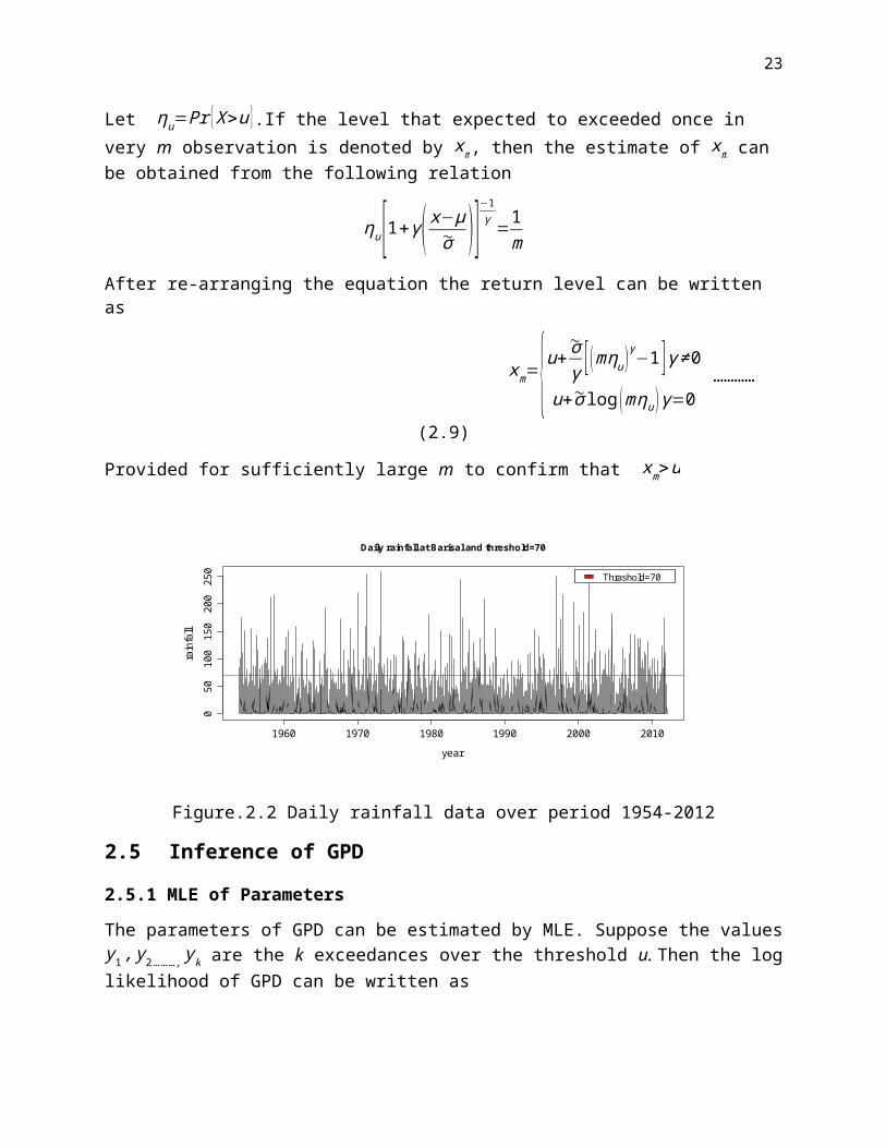
Daily rainfall at Barisal and threshold=70

year

rain

fall

1960 1970 1980 1990 2000 2010

050

100

150

200

250 Thrashold=70Thrashold=70Thrashold=70

17

Figure.2.2 Daily rainfall data over period 1954-2012

2.5 Inference of GPD

2.5.1 MLE of Parameters

The parameters of GPD can be estimated by MLE. Suppose the values y1 , y2………, yk are the kexceedances over the threshold u.Then the log likelihood of GPD can be written as

l (~σ , γ )={−klogσ−(1+ 1γ )∑k=1

k

log(1+γ y i~σ ) for γ ≠0

−klog~σ−~σ−1∑i=1

k

y i for γ=0

provided that (1+σ−1 γ y i )>0 for i=1,2 ,… .., k

Replacing the MLE of ~σ , γin eq (2.9) , the MLE of return level is obtained and the estimates of

ηu can be found by ηu=kn . The 95% CI of parameters derived using delta and profile likelihood

methods. From the properties of binomial distribution we get the variance of ^(η¿¿u)≈

ηu(1−ηu)n

¿¿.

Therefore the variance-covariance matrix of (ηu ,~σ , γ) is approximately

[ ηu(1−ηu)n

0 0

0 v1,1 v1,2

0 v2,1 v2,2]

Here vi , j denotes the (i,j)th term of the covariance matrix of ~σ∧ γ.

By delta method , var ( xm )≈∇ xmT V ∇ xm

Where ∇ xmT =[ δ xm

δ ηu,δ xm

δσ,δ xm

δγ ] =[~σ mγηu

γ−1 , γ−1 ( (mηu )γ−1) ,−~σ γ−2 ( (mηu )γ−1)+σ γ−1 ( (mηu )γ log (mηu )) ]evaluated at (ηu ,~σ , γ) .[21]

2.6Connection with Poisson Distribution: Poisson-GPD Model forExceedances

The Poisson-GPD model is used to explain the connection between the PoT and Block Maxima methods. This useful model in extreme value theory is a limiting form of joint process of

18

exceedances time and excess over threshold. The straightforward connection between the GEV and GPD models can be explained in such a way that if the number of exceedances over u per year follows Poisson distribution with mean λ, and if the exceedance distribution falls within the generalized Pareto family with shape parameter γ, then the annual maximum distribution falls within the GEV family with the same shape parameter. Another one-one relation between (λ, σ) and (μ, ~σ) that is the location and scale parameters of the annual maximum GEV distribution. The essential benefit of inference on the annual maximum distribution is now derived from a greater amount of information that increased precision.

The relation between GEV and Poisson –GPD is found by following these steps. Suppose x>u. The probability that the annual maximum of the Poisson-GPD process is less than x is

Pr {max1≤i≤ N

Y i≤x }=Pr {N=0 }+∑n=1

∞

Pr {N=n ,Y 1≤x ,……. ,Y n≤x }

¿e− λ+∑n=1

∞ λn e− λ

n!¿¿¿

¿exp {−λ(1+γ x−uσ )

−1γ }

This is GEV with σ=σ+γ (u−μ ) and λ=(1+γ u−μσ )

−1γ .

Thus the GEV and GPD models are completely consistent with one another above the GPD threshold u .It also indicates how the Poisson–GPD parameters σ and λ vary with the change of u.[22]

2.7 Extremal Index: Measures of StationaritySmith et al. (1997) [23] used geometric distribution to model the cluster length of low minimum daily temperatures. The probability mass function of Geometric distribution is defined as

f ( t ,θ )=θ (1−θ )t−1 ,t=1,2 ,…

Here θ is known as extremal index and the reciprocal of the parameter θ is mean. This extremal index used measure the tendency of clusters of extreme events under stationary process. For stationary series the lower value of θ, is, the higher local dependence exists as well as higher tendency to clustering at extremal levels. In this thesis we model the time lag between two extreme rainfalls over threshold u as a geometric distribution to checks stationarity of the rainfall series.[21]

2.8 Model Validation

Model validation is an important tool to check how well the model suits the data or the data actually came from the assumed model. There are several ways to check accuracy of model and some of them which we used in this thesis to check model are explain in the following section.

2.8.1 quantile-quantile (q-q) plot

19

The quantile-quantile (q-q) is one of the common tools used to check models. The plot is constructed by using the points

{( F−1( in+1 ) , x(i)): i=1,2 ,……… ..n}

F−1( in+1 ) and x (i )both provide the estimates of ( i

n+1 ) thquantile of distribution F. The diagonal

QQ plots confirm that F is a good estimate of F.

2.8.2 Goodness of fit test

The goodness of fit (GoF) test is used to check how well a theoretical probability distribution or statistical model fits the observed data. The GoF index summarizes the inconsistency between observed and expected value under a specified model. This approach is widely used to test normality of residuals or to test whether two samples are drawn from identical distribution or the outcome frequency follows a specified distribution (Pearson chi square). Therefore Pearson’s chi square test is used to test the null hypothesis that the frequency distribution observed in a sample follows particular theoretical distribution.

χk− p−12 =∑

k

( f o−f e)2

f e

f o=observed frequaency

f e=theoritical frequency

The null hypothesis is rejected if χk− p−12 >Cα where c is the (1−α ) th quantile of χk−p−1

2 distribution.[24]

2.8.3 Likelihood Ratio Test

Likelihood ratio test is used to compare between two nested models. Asymptotically, the test statistic is distributed as a chi-squared random variable, with degrees of freedom equal to the difference in the number of parameters between the two models. Models that are to be compared with each other have to be a restricted version of the other model. If the restricted model has m different restrictions on the value of the parameter vector θ then restricted model is called the null model while the unrestricted model is called the alternative model. After fitting model to the data log-likelihood functions are maximized under restricted and unrestricted model assumption respectively. The maximized log-likelihood for the null model is l (θ0 )and l (θ1 )denotes the maximized log-likelihood for the alternative model, then

D=2(l (θ0 )−l (θ1 )) χ m2

D is known as deviance function and the null model is rejected in favor of the alternative model if D>Cα where Cα is the (1−α ) thquantile of χm

2 distribution. [21]

20

Chapter 3

Multivariate ExtremeThe Multivariate extremes used to characterize the dependence of extreme events or determine how the extremes relate to each other. Therefore multivariate modeling framework basically divided in to two distinct steps. Firstly modeling univariate margins and then at second steps using proper standardization of margins the dependence is modeled. The basic assumption is that the dependence structure of the underlying distribution may at extreme levels can be approximated by a max-stable dependence structure. In this section we describe multivariate extreme value models and its dependence structure concerning both parametric and non-parametric estimation approach. Both the component wise maxima and threshold approach are discussed.

3.1 Dependence Measures

Correlation refers the strength of the dependence between two variables. In this thesis we have used two kinds of dependence measures. Pearson’s rho is the most used as the linear correlation and the other one is Kendall’s tau based on rank correlations. In the following we will give a brief explanation about these two dependence measures.

3.1.1 Pearson’s Rho

Pearson’s correlation is the most broadly used measure to find linear correlation between two variables. It can be denoted as ρ and defined as:

ρ=cov (X ,Y )

√V (X)V (Y )Properties

Correlation coefficient, ρ varies -1 to 1 and -1 indicates a perfect negative linear relationship between variables, 0 indicates no linear relationship between variables, and an 1 indicates a perfect positive linear relationship between variables.

Sensitive to outliers. Invariant only under strictly increasing linear transformations.Scatter plots are drawn using this correlation measure.

3.1.2 Kendall Tau

Kendall’s tau is a measure of non-parametric rank correlations assess statistical association based on the ranks of the data. Suppose two variables (X1 ,Y 1 ) and (X2 ,Y 2 ) are independent and idenetical distributed random vectors, with joint distribution function H. The concordance and discordance probability can be defined asConcordance probability: P ((X1−X2)(Y 1−Y 2)> 0) Discordance probability: P ((X1−X2)(Y 1−Y 2)<0) Then Kendall tau can be obtained by

21

τ=¿P ((X1−X2)(Y 1−Y 2)> 0)- P ((X1−X2)(Y 1−Y 2)<0)

Therefore the Kendall’s tau is the difference between concordance probability and discordance probability.

Properties Correlation coefficients, take the values between minus one and plus one. The positive correlation signifies that the ranks of both the variables are increasing. The negative correlation signifies that as the rank of one variable is increased, the rank

of the other variable is decreased.

Concordant Pair: Both members of one observation are larger than their respective members of the other observations.Discordant pairs: The two numbers in one observation differ in opposite directions.[25]

3.2 Max-Stable and Max-Infinite Divisibility According to the theory of univariate extreme value for a positive integer k there exists vectors α k>0 and βk such that an

−1(ank )→α k and an−1(bnk−bn)→βk as n→∞.Moreover we have

Fnk (ank x+bnk )→G ( x )as n→∞.Then we obtain

Gk (α k x+βk )→G ( x ) x∈ Rd……………….(3.1)

Here G(x ) is a d-variate distribution function and for every positive integer k there exists α k>0 and βk such that equation (3.1) is true then it is known as Max-stable. Equation 3.1 can be interpreted as if Y 1 ,Y 2………are independent random vectors with distribution function G then

α k−1 (¿ i=1¿k Y i−βk )≝Y ,k=1,2,3...

Using results of (3.1) it can be said that for every positive k G1k is a distribution function, then G

is max-infinitely divisible. Specifically for a measure μ defined on [-∞ ,∞) such that

G ( x )=exp {−μ (¿∖ [−∞ ,x ])}, x∈ [−∞ ,∞ ]…………….(3.2)

In order to study the dependence structure of max-stable distribution, it is convenient to use unit Fréchet distribution margins hence the exponent measure must satisfy homogeneity property.

Let the distribution function of d-variate random vector Y is G and G j is the j-th margins and G j

q is the quantile function of G j that can be written as G jq=x where 0<q<1.Then

G j=exp¿ x j∈Rd

G jq(e

−1x j )=μ j+σ j

z jγ j−1γ j

, 0<z j<∞

Suppose the distribution function of( −1log (G1)

,………, −1log (Gd))is G* which can be written as

22

G¿ ( z )=G {G1q(e

−1z1 ),………,Gd

q (e−1zd )}z>0

and G ( x )=G¿¿

For any positive integer k and j=1,2 ,…….d following relation is true

G jk (α kj x j+βkj )=G j (x j )

Then G¿ is a max-stable as well as all margins are max-stable which follows that

G¿k (kz )=G¿ (z) z∈Rd and k=1,2 ,….

If μ¿ is a measure of extreme value distribution with unit Fréchet margins then we have

−logG¿ ( z )=μ¿ (¿∖ [0 , z ] ), z∈ ¿

which leads to μ (¿∖ [q , x ])=−logG (x )=−logG¿ ( z )=μ¿ (¿∖ [ 0 , z ]),

where z∈ [ 0 ,∞ )and x ∈[q ,∞ ]

Therefore multivariate extreme value distribution can be given with Unit Fréchet margins. For simplicity here considering bivariate case, then bivariate extreme value distribution denoted by G¿(x,y) with unit Fréchet margins can be written as

G¿( x . y)=exp−μ¿ [0 , ( x , y ) ]c where μ¿ [0 , ( x , y ) ]c=( 1x+ 1y )A ( x

x+ y )and A (ω )=∫

0

1

max {q (1−ω ), (1−q )ω} S (dq )

The conditions for measurement of Sis that

∫0

1

qS (dq )=∫0

1

(1−q )S (dq )=1

The function A (ω ) is called dependence function that used to estimate dependence between two extreme variables and satisfy the following conditions

A (0 )=A (1 )=1 max {ω, (1−ω ) }≤ A (ω )≤1 A (ω ) is convex for ω∈ [ 0,1 ]

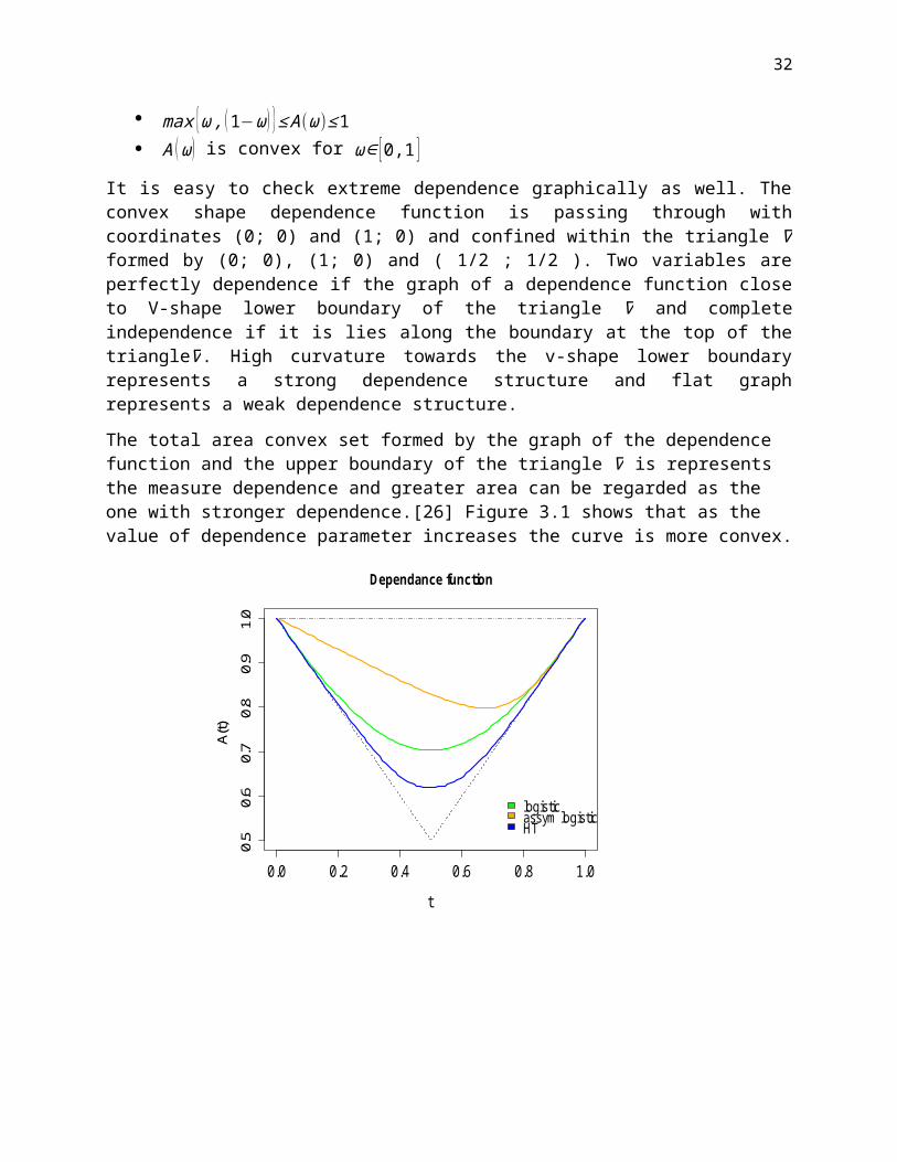
It is easy to check extreme dependence graphically as well. The convex shape dependence function is passing through with coordinates (0; 0) and (1; 0) and confined within the triangle ∇ formed by (0; 0), (1; 0) and ( 1/2 ; 1/2 ). Two variables are perfectly dependence if the graph of a dependence function close to V-shape lower boundary of the triangle ∇ and complete independence if it is lies along the boundary at the top of the triangle∇. High curvature towards the v-shape lower boundary represents a strong dependence structure and flat graph represents a weak dependence structure.

23

The total area convex set formed by the graph of the dependence function and the upper boundary of the triangle ∇ is represents the measure dependence and greater area can be regarded as the one with stronger dependence.[26] Figure 3.1 shows that as the value of dependence parameter increases the curve is more convex.

Figure 3.1. Dependence function plots of 2000 simulated data from logistic (dep=.5), asymmetric model with parameter (dep=0.1, asy=c(0.2,0.8)) and non-parametric HT dependence at 0.3.

3.3. Component Wise MaximaBarnett (1976) considers several different categories among them Component wise ordering is considered here. Suppose for d-dimensional vectors x = (x1 , x2,……xd) and ¿ the relation x≤ y is defined as x j≤ y j for all j=1,2 ,…….d . The component wise maxima can be defined as

x⋁ y=(x1∨ y1, x2∨ y2 ,…… xd∨ yd )

where ∨stands for the maximum (analogously, a ∧ b = min(a, b)). By using this notation the maximum of a sample of d-dimensional observations

X i=(X i ,1 , X i ,2 ,………X i , d ) for i=1,2 ,……. ,n is defined as

M n=(M n , 1 , M n ,2 ,………M n , d )¿¿ i=1¿n X i ,1 ,……….¿ i=1 ¿n X i , d

Therefore it can possible to focus on maximum without loss of generality, since the following relation allows us to get the minimum by the help of the maximum of the negatives

¿ i=1¿n X i ,1=−¿ i=1¿n (−X i ,1 )

3.4 Density Function of BEVD

0.0 0.2 0.4 0.6 0.8 1.0

0.5

0.6

0.7

0.8

0.9

1.0

Dependance function

t

A(t)

logisticassym logisticHT

24

Now (X1 , X2) denote a bivariate random vector representing the component-wise maxima of an i.i.d. sequence over a given period of time. Under the suitable conditions the distribution of (X1 , X2) can be approximated by a bivariate extreme value distribution (BEVD) with cdf G. The BEVD is determined by its two margins G1 and G2 respectively and these margins are distributed as EVD. Suppose dependence function is A

Then G (X1 , X2 )=exp {logG1(x1)G2(x2)A ( logG2(x2)logG1(x1)G2(x2))}………..(3.3)

By probability integral transformationU i=Gi (X i), i=1 ,2 we obtain uniformly distributed variables on the unit interval that can easily be further transformed to any chosen distribution. So now BEVD expressed assuming standard exponential margins.

Let us denote Y i=T i (X i )=−log (U i ) , i=1 ,2

Then the joint survival of the new vector (Y 1 ,Y 2)) can be written as

G¿ ( y1 , y2)=P (Y 1> y1, Y 2> y2 )

¿P (−logG1 (X1 )> y1 ,−logG2 (X2 )> y2 )

¿P (X1<G1−1 (e y1 ) , X2<G2

−1 (e y2) )

¿exp{−( y1+ y2 ) A ( y2

y1+ y2 )}……………………… (3.4)

where * denotes the marginal change in the distribution. To obtain the density of BEVD one needs the first and second derivatives of the dependence function denoted by A'( ⋅ ) and A" ( ⋅ ) respectively. The density (on the original scale) can be expressed

g (x1 , x2 )= δ 2

δx1 δ x2G1 (x1 , x2 ) ………… (3.5)

¿ δ 2

δx1 δ x2G¿ (T 1 ( X1 ) ,T 2 ( X2 ))

¿G¿ (T 1 ( X1 ) ,T 2 (X2 )) (T 1' (X1 ) , T2

' (X2 ))×

( (A (ζ )+(1−ζ ) A ' (ζ ) )( A (ζ )−ζ A ' (ζ ) )+η A ' ' (ζ ) )

where T i ( x )=−logGi ( x )=(1+γ ix−μi

σ i)−1γ i , i=1,2

T 'i ( x )=−1

σ i(1+γi

x−μ i

σ i)−1γi

−1, i=1,2

25

ζ=T 2 ( x2 )

T 1 (x1 )+T 2 ( x2 )

η=T 1 (x1 )T 2 (x2)

(T1 (x1 )+T2 (x2 )3)

So for BEVD density, the condition is that A( t) is two times differentiable. The usual parametric models satisfy this property as well, but for non-parametric estimates it becomes more problematic A( t).[26]

3.5 Measures of Extreme Dependence There are several approach like the exponent measures, spectral measures, the stable tail dependence function, copula and non-parametric estimator used to explain dependence structure (A (t )¿of a max stable distribution. In this thesis we have used two parametric stable tail dependence function and non-parametric dependence function to explain the dependence of extreme rainfall.

3.5.1 Parametric Models

Logistic model

The oldest parametric family of bivariate extreme value dependence structures introduced by Gumbel (1960) is logistic model and stable tail dependence function can be written as

l (v1 , v2 )=(v1

1r+v2

1r ) v j>0 j=1,2

The parameter r (0 < r ≤ 1) measures the strength of dependence between the two coordinates and r=1 correspond independence and r ↓ 0 is complete dependence. The strength of dependence increases as r decreases.

Asymmetric logistic models

An asymmetric logistic model proposed by Tawn (1988), is

l (v1 , v2 )=(1−ψ1 )v1+ (1−ψ2 )v2+{(ψ1 v1 )1r+(ψ2v2 )

1r }r v j> 0 , j=1,2

And 0<r<1 and 0< ψ j<1 .For ψ1=ψ2 explains mixture of independence and reduced as the logistic model specifically ψ1=ψ2 = 1. If r = 1 or ψ1= 0 or ψ2 = 0 reveals independence and r < 1, Complete dependence arises if ψ1=ψ2 = 1.

3.5.2 Non-Parameter estimation

HT estimator

26

Hall and Tajvidi (2000) proposed the estimator to approximate an arbitrary initial estimator by a polynomial smoothing spline of degree three or more, the knots being equally spaced on the unit interval. Let the random pair (X ,Y ) have distribution functionG¿ in equation 3.3 with continuous margins G1and G2and the joint survival function is equation 3.4. Let (Y 1 , j ,Y 2 , j) , j=1,2 ,… ..n

denote a vector sample from (Y 1 ,Y 2) and Y 1=

∑j=1

n

Y i , j

n ,i=1,2 the HT estimator can be expressed

as follows

1A k

HT (t )=1

n∑i=1

n

min( Y 1 , j

Y 1

1−t,

Y 2 , j

Y 2

t ) t∈[0,1]

and it satisfies AkHT (0 )= Ak

HT (1 )=1 and AkHT(t )≥max (t ,1−t )

Capéraà Fougères-Genest (CFG) estimator

Proposed by Capéraà etal. (1997). Let (Y 1 ,Y 2) be a bivariate standard exponential pair with joint survival function given by (3.4). Then

P [max {t Y 1, (1−t )Y 2 }>x ]

¿P[Y 1>xt ]+P[Y 2>

x(1−t ) ]−P [Y 1>

xt,Y 2>

x(1−t ) ]

¿exp(−xt )+exp { −x

(1−t ) }−exp [−xA (t){t (1−t ) } ]

Here t∈ [0,1 ] and x>0. Therefore it can be written that

E [logmax {t Y 1 , (1−t )Y 2 }]=logA ( t )+∫0

∞

log (x)e−x dx

Now A( t) can be estimated empirically by following steps

log Ak ( t )=1n∑j=1

n

logmax {t Y 1 , j , (1−t )Y 2 , j }−∫0

∞

log (x)e− xdx

Though this estimator does not satisfy the constraint A(0)=A (1)=1,after some modification

the dependence estimator named as CFG defined as follows

log AkC (t )=log Ak (t )−tlog A k (1 )−(1−t) log A k (0)

¿ 1n∑j=1

n

log max {t Y 1 , j , (1−t )Y 2 , j }−t 1n∑j=1

n

logY 1 , j−(1−t ) 1n∑j=1

n

log Y 2 , j

[26]

27

28

3.6 Multivariate Generalized Pareto Distribution

The idea of the multivariate extreme value distribution is suggested by Tajvidi and then has been developed Rootzén and Tajvidi.[16] The statistical properties of these models have not been studied completely yet as to our best knowledge .In component-wise maxima, we do not have information about the time of occurrence extremes or the maxima occurred concurrently or in the same day. To overcome these problems the multivariate peaks over threshold methods are used to investigate all observations exceeding a given high threshold. This is a great scope of having more accurate estimation using more data.

The definition of the multivariate generalized Pareto distribution by Rootzen and Tajvidi (2006) are stated as follows

Definition 2.1: A distribution function H is a multivariate generalized Pareto distribution if

H ( x )= 1−logG (0 )

log G (x )G ( x⋀ 0 )

……………………….(3.6)

for some extreme value distribution G with non-degenerate margins and with 0¿G(0)<1.

Specifically,H (x )=0 for x<0 and H (x )=1− logG(x )logG(0) for x>0.

Here given some remarks about MGPD

Remark 1: The definition of MGPD does not suggest the lower dimensional margins of MGPD are not GPD’s. Nevertheless, if Z is distributed as H then the conditional distribution of f (Z i∨Z i)>0 is GPD. In any dimension less then d, all marginal distributions hold this property.

If X be a d-dimensional random vector with distribution functionF, {u (t):t∈¿ } a d-dimensional curve starting at u (1 )=0and σ (u )=σ (u( t))>0 be a function with values in Rd. The normalized exceedances (Xu at level u then it can be defined as

Xu=X−uσ (u )

Theorem 3.1 i. Suppose, that G is a d-dimensional EV distribution with0<G (0 )<1. If F∈D (G )then

there exist an increasing continuous curve u with F (u(t))→1 as t →∞ and a function σ (u )>0 such that

P (Xu≤x ∕ Xu≤S 0 )→ 1−logG (0 )

log G ( x )G ( x⋀ 0 )

as t→∞ for all x.

29

ii. Suppose there exists an increasing continuous curve u withF (u(t))→1 as t →∞ and a functionσ (u )>0 such that

P (Xu≤x ∕ Xu≤S 0 )→H (x),…………..(3.7)

for some function H , as t →∞, for x>0, where the marginals of H on R+¿ ¿ are non-degenerate. Then the left hand side of (4) converges to a limit H (x ) for all x and there is a unique multivariate extreme value distribution Gwith G(0)=e−1 such that

H (x )=logG(x )

logG (x⋀ 0)

This G satisfies G ( x )=e−H (x) for x>0, and F∈D (G ).

Theorem 3.2i. Suppose X follows multivariate generalized Pareto distribution then there exists an

increasing continuous curve u with P(X<u(t))→1 as t→1, and a function σ (u )>0 such that

P (Xu≤x ∕ Xu≤S 0 )=P(X ≤ x) for t∈ ¿ and all x……… ……(3.6)

ii. If there exists an increasing continuous curveu with P(X<u(t))→1 as t→∞, and a function σ (u )>0 such that equation 3.6 holds for x>0, and X has nondegenerate margins, then X has a multivariate generalized Pareto distribution.

3.7 Density Function of BGPD Models

Let (Z1 ,Z2 ) be the random variable, (u1 ,u2) a given threshold vector and the random vector of exceedances is (X1 , X2)= (Z1 - u1, Z2−u2) We define the bivariate generalized Pareto distribution (BGPD) for the exceedances by its cdf (theorem 3.1)

H (x1, x2 )= 1−logG ( 0,0 )

logG ( x1 , x2 )

G (x1 ,⋀0 , x2⋀ 0 )

for some BEVD, G with non-degenerate margins and with 0<G(0 ,0)<1. So practically the probability measure is positive in the upper three quarter planes and zero in the bottom left one. The definition refers that the BGPD distribution models those observations too, which are extremes merely in one component. The h density of BGPD is easily obtainable by straightforward computations and it can be expressed with the terms of (3.5)

h (x1 , x2 )=T 1

, (x1 )T 2' (x2 )

c0×η A, , (ζ )

where T i ( x )=−logGi ( x )=(1+γ ix−μi

σ i)−1γ i , i=1,2

30

T 'i ( x )=−1

σ i(1+γi

x−μ i

σ i)−1γi

−1, i=1,2

ζ=T 2 ( x2 )

T 1 (x1 )+T 2 ( x2 )

η=T 1 (x1 )T 2 (x2)

(T1 (x1 )+T2 (x2 )3 )

c0=−(T 1 (0 )+T2 (0 ))A( T 2 (0 )T 1 ( 0 )+T2 (0 ) ) [27,28]

31

Chapter 4

Data and Rainfall Pattern of Studied Stations

4.1 DataThe daily maximum rainfall data recorded at five meteorological stations were collected from the Bangladesh Meteorological Department (BMD). Each station signifies one district (mid-level administrative unit in Bangladesh) and 3 of them in coastal region and rest two are from northern part of Bangladesh. There are some missing data the early periods and in 1971(liberation war period), we omit these missing data before analysis.

Statistical packages: All estimation and calculation in empirical analysis are implemented in R with packages fitdistrplus,in2extRemes,evd.

4.2 Overview of Rainfall We briefly discuss about the daily rainfall pattern by studying plots and some summary statistics of the studied stations over the entire period. According to Köppen and Geiger, the climate of Barisal, Khulna, Bogra and Satkhira are classified as tropical savanna climates(Aw). Tropical wet and dry or savanna climate (Aw) can be defined as a distinct dry season, with the driest month having precipitation less than 60 mm and less than 1/25 of the total annual precipitation. So annual maximum rainfall are from wet seasons and very little during dry seasons. [29]

4.2.1 Station Barisal

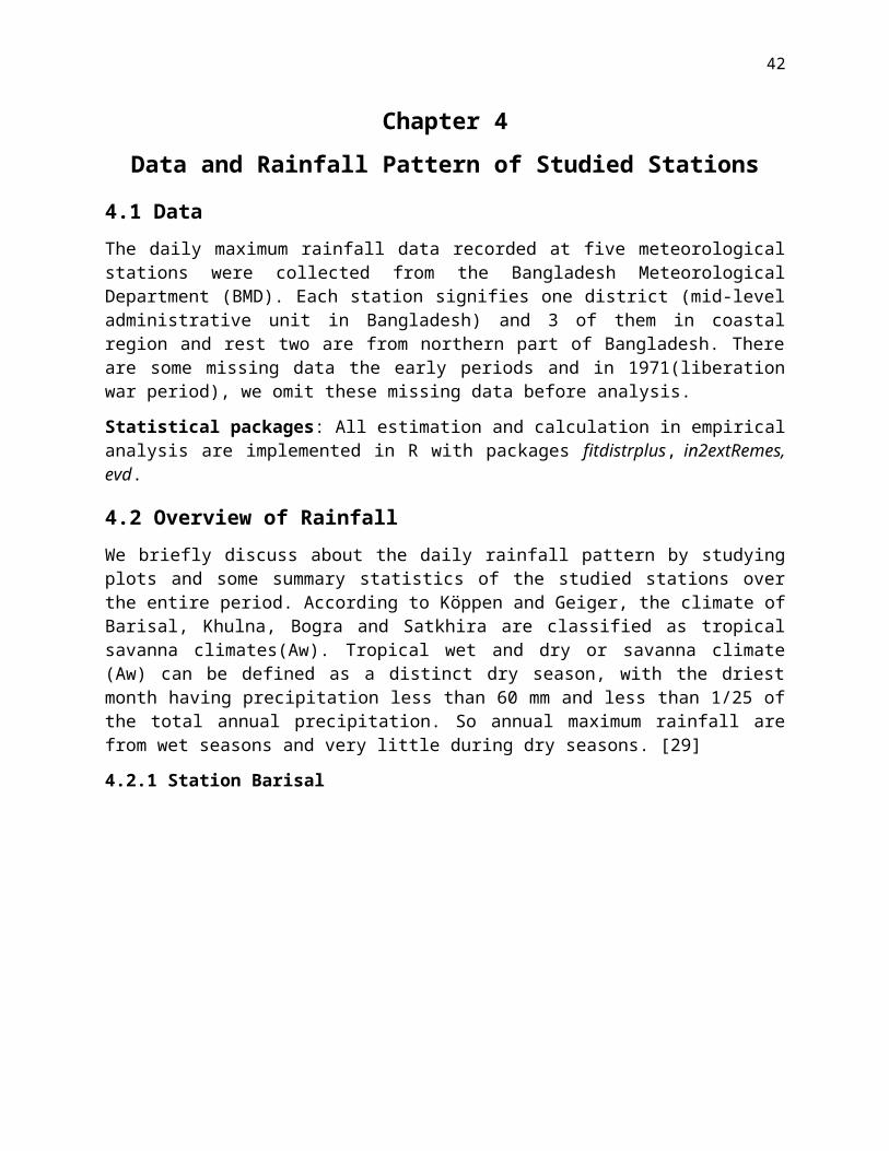
Barisal is located in south-central Bangladesh and crisscrossed by plenty of rivers and the average annual rainfall is 2184 mm. The driest month is January having 10 mm of rainfall and the most precipitation falls in average 444 mm during July. [29]

Figure 4.1. Annual maximum rainfall and number of zero rainfall per year over 1954-2012

Yearly rainfall at Barisal

Year

Rai

nfal

l

1960 1970 1980 1990 2000 2010

5015

025

035

0

zero rainfallmax rainfall

32

The maximum rainfall in this area during study period is 258 mm which occur in 1967. Annual maximum rainfall and days with zero rainfall versus year are plot is Figure 4.1. At the beginning of study period the maximum rainfall and days with zero rainfall per year are high. But the maximum rainfall has been decreasing after 1990 except the years 1998 and 2004. Bangladesh has affected by severe flood during these two year. After 2002 the number days with zero rainfall are increasing. Climate researchers identified global warming is responsible for this pattern of rainfall. The maximum rainfall looks reasonable for assuming the variation over time periods has constant.

4.2.2 Station Khulna

The average annual rainfall is 1736 mm at Khulna. The lowest precipitation is in average of 6 mm in December and Most of the precipitation recorded in July on average 357 mm. [29]The maximum rainfall at this station is 430 mm which occur in 1986.The range of annual maxima over this time period varies within the range (52mm-430mm). After 2001 maximum rainfall has been decreasing and total number of days with zero rainfall increasing. Due to global warming this type of rainfall pattern are very risky for natural disaster (Appendix Figure A4)

4.2.3 Station Satkhira

The average annual amount of precipitation in Satkhira 1689.1 mm and the month with the most precipitation on average is July with 353.1 mm of precipitation. The month with the least precipitation on average is January with an average of 7.6 mm and The Bay of Bengal is the south border of Satkhira.[29] The maximum rainfall at this station is 302 mm which occurred in 1986. Annual maximum rainfall and number of days per year with no rainfall at station Satkhira over time 1954-2012 is presented in Figure A5 (Appendix). The rainfall recorded at this stations having nice pattern. At the beginning of the study period the annual maximum rainfall and the days with zero rainfall were large. After in the 1990 the maximum rainfall per year has been decreasing and days with zero rainfall increasing.

4.2.4 Station Bogra

Average precipitation at Bogra is 1762 mm. The driest month is December, with 6 mm of rain. With an average of 397 mm, the most precipitation falls in July.[29]

The maximum rainfall at this station is 279 mm which was in 1988. The maximum rainfall in this area are decreasing year after 2000 except 2007 and 2011 and the days with zero rainfall have been increasing after 1993.Due to these zero rainfall this station have risk of drought-related vulnerability. The Figure A6 (Appendix) shows maximum annual rainfall and the number of zero rainfall by year. The maximum rainfall plot looks reasonable to assuming that the pattern of rainfall is stationary and modeled as a GEV distribution.

4.2.5 Station Rangpur

Rangpur is the northern part of Bangladesh climate is classified as warm and temperate. The summers are much rainier than the winters in Rangpur. According to Köppen and Geiger, this climate is classified as Cwa i.e Mild with dry winter, hot and wet summer. The average annual rainfall is 2192 mm. Precipitation is the lowest in December, with an average of 6 mm. Most of the precipitation here falls in July, averaging 357 mm.[29] Annual maximum rainfall and number

33

of days with zero rainfall recorded at station Rangpur over time 1954-2012 is presented in Figure A7 (Appendix).The maximum 294 mm rainfall that occurred in 2002.The number of days with no rainfall over the entire period are very large except few years.

4.3 Empirical Upper Quantiles

Empirical quantiles for daily rainfall in Table 4.1 shows long tail of the rain fall data. This empirical quantile statistics is an overview of end data pattern and reveals that the daily rainfall data have a long tail. Also 95% rainfall for stations Khulna, Satkhira and Bogra stations are below 30 mm

Table 4.1. Empirical upper quantiles for daily rainfall (mm)Quantile 95% 96% 97% 98% 99% Max MinBarisal 35 40 46 56 77 258 0Khulna 29 33 39 51 72 430 0Satkhira 27 32 38 48 65 302 0Bogra 29 34 40.79 52 71 279 0Rangpur 35 41 50 66.74 88 294 0

34

Chapter 5

Analysis of Rainfall

Throughout this chapter we investigate the series of daily rainfall data over period 1954-2012 recorded different stations of Bangladesh. In part A, we discuss two univariate extreme value distributions namely GEV and GPD to find the distribution rainfall. In part B we investigate bivariate dependence structure between stations using margins obtained from A. Two models bivariate extreme value distribution and Bivariate Generalized Pareto distribution are used in the analysis.

5.1 Method of Finding Suitable ModelsAlready mentioned the daily maximum rainfall data recorded from five different stations over period 1954-2012 are investigate here .Trend and stationary should be checked before modeling the rainfall data. These can be done by fitting Poisson distribution and geometric distribution respectively. The annual maximum rainfall data of each can be modeled as GEV separately in block maxima approach. Different model checking tools like density plots, qq-plots are applied to the fitted model to check suitability of series to the data. MLE of the parameters estimated and 95% CI by both delta and profile likelihood are estimated .The value of shape parameter ( γ ¿is an indication about the tail of distribution .The return levels of 10,50 and 100 years return periods are estimated. These statistics are very useful measure to have approximate idea about the risk of having that level rainfall next 10, 50 or 100 years. Also 95% CI estimated both delta and profile likelihood methods and compare. This asymmetry shape CI implies that the data provide gradually weaker information about the high levels of the process.

Another useful model in the extreme value theory is GPD model that used to model daily rainfall data. Here also GPD is fitted separately for all stations. The peaks over threshold method apply in GPD modeling approach. More clearly, the exceedances over a fixed threshold are modeled as GPD. So we have to be more careful in selecting a threshold. Both Mean residual plot and threshold range plots are applied to find appropriate threshold. Then GPD model is fitted to the exceedances and model diagnostic tools are used to check the performance of models. MLE of parameters and 95% CI are estimated. Using the MLE of parameters the 10, 20 and 100 years return levels are estimated. Both delta and profile likelihood methods are applied to estimate 95% CI.

After univariate modeling of rainfall data then we go for bivariate extreme value distributions are considered to check the dependency between rainfalls of two stations. For this purpose we use component wise block maxima approach and bivariate peaks over threshold methods. Merging annual rainfall data by year and BEVD is used to model component-wise yearly maximum rainfall for both stations. Both Parametric bivariate logistic and bivariate asymmetric logistic dependence structure are used to model tail dependence considering margins are from GEV distribution. As well as some non-parametric estimators of the dependence functions CFG and HT (Hall and Tajvidi) are also estimated. Test for independence between margins based on score statistics suggested by Tawn(1988) [18] also performed for all stations. The strength of dependence can found by estimating d = 2(1- A(1/2)) and d∈ [0,1]. The lower limit implies independence and complete dependence between observations indicating by upper limit .The

35

dependence plots also an important tool for identifying dependence graphically which also performed for all pairs of stations .The quantile plots also shows the upper quantiles of joint distribution and we can get idea about the return levels for both margins.

Bivariate peaks over threshold approach also applied here. After fixing threshold and parametric models (logistic and asymmetric logistic) are consider to model the dependence and the estimated strength of dependence between stations. The dependence plots and quantile curve also used as a tool for checking the dependence structure of the daily rainfall data.

Part A: Univariate Extreme Value Modeling

5.2 Univariate Extreme Value AnalysesIn both GEV and GPD models we use maximum likelihood method to estimate the parameter. Confidence interval estimation using both delta and profile likelihood methods and return levels with confidence interval are briefly explained in this section.

5.2.1 Stationarity and Trend Checking

Geometric distribution is fitted using the data of time lag between two exceedances over threshold. Chi –square goodness fit performs and all p-value are greater than 0.05. Moreover model checking qq plots and histograms of the data also approximately accurate and all results are not presented here.

The total number of exceedances per year over a fixed threshold modeled as a Poisson distribution and the summary statistics of Poisson fit are presented in the Table 5.1. Stations Barisal have maximum intensity of extreme rainfall among this five stations .The p-value from good ness of fit test are greater than 0.05 indicating the good fit of Poisson distribution. So the data are free of trends. Model checking plots are okay for Poisson distribution.

Table 5.1: Summary of Poisson fit for 5 stationsStation Threshold Intensity(λ) p-valueBarisal 90 2.379 (0.203) 0.847Khulna 110 0.929(0.1288) 0.294Satkhira 90 1.597(0.1674) 0.362Bogra 85 2.373(0.201) 0.128Rangpur 115 1.877(0.182) 0.180

36

5.2.2 Threshold selection for GPD

Threshold range plots for daily rainfall data at Barisal shown Figure A3(Appendix), exhibits stability in both parameters at u=90.Mean residual plots with approximate 95% confidence interval for daily rainfall data shown in Figure A2(Appendix).The mean residual plots appears to curve from u=0 to u=40, after that it is approximately linear until u=90.So we can fix 90 as a threshold. In addition, over threshold (u)=90 the number of exceedances follow Poisson distribution . Similarly we have found threshold for Khulna, Satkhira, Bogra and Rangpur using respective daily rainfall data. The threshold for Khulna is 110 for Satkhira is 90, 115 for both Rangpur and 85 for Bogra.

5.2.3 Model Checking Plots

The Model checking qq-plots of the empirical versus fitted models are reasonably linear and the density plots indicate that the assumptions for using the GPD and GEV are fulfilled for all station

5.2.4 Parameter Estimation

Maximum likelihood estimation (MLE) method is used to estimate parameters of GEV distribution and the parameters with confidence intervals estimated by both delta method and profile likelihood are presented in the following Table 5.2.Profile likelihood CI usually provide better accuracy in estimating confidence interval which are slightly different from delta method. So here we only present profile likelihood CI.

For station Barisal the estimated GEV shape is negative i.e γ ¿0 which refers to type III,

Weibull classes and the support of the GEV distribution is bounded from by μ−σγ=639.2547

mm. Hence it can be interpreted as the predicted future rainfall for any return period should never be greater than 639.2547 mm. The strength of evidence from the data for a bounded distribution is not strong as 95% CI extends above zero.Shape parameter of GPD is approximately equal and standard errors are smaller compared to GEV and like GEV CI are not exactly in the positive domain. The standard error of estimated parameters is small.

The shape parameters of both GEV and GPD obtained by fitting rainfall at Khulna are approximately equal and positive i.e. γ ¿0 .The rainfall follows GEV distribution of type II (Fréchet family) with no upper bound. The standard errors of estimated parameters of GPD are larger compared to GEV model.

The rainfall at Satkhira follows type III GEV as the MLE of shape parameters is negative i.e. γ

¿0.We can estimate the upper end point μ−σγ=¿ 1279.09 mm but 95% CI are above zero so the

inference is not so strong. Furthermore MLE of GPD shape is zero that is the indication of infinite range of rainfall.

37

The estimated scale from both distributions is nearly equal at station Bogra. Shape parameters is positive i.e. γ ¿0so this is GEV distribution of type II which is known as Fréchet family with heavy tail and has no upper end point. Also GPD fit shows the rainfall have infinite range.

Negative shape indicates that the distribution of rainfall at Rangpur is bounded but the inference is not strong since the upper bound of CI are above zero.

Table 5.2. Summary of GEV and GPD fit Station GEV GPD

Location (μ) Scale (σ ) Shape(γ) Scale (σ ) Shape(γ)Barisal Estimate(sd) 122.36(6.507) 43.29(4.68) -0.084(0.109) 42.83(5.425) -0.066(0.094)

LCI 111.58 35.66 -0.295 33.27 -0.2279UCI 135.88 54.67 0.144 54.65 0.1458

Khulna Estimate(sd) 103.29(5.85) 38.86(4.69) 0.225(0.107) 36.09(8.54) 0.301(0.197)LCI 92.48 31.023 0.045 22.27 0UCI 115.44 49.750 0.465 56.52 0.790

Satkhira Estimate(sd) 101.59(6.90) 47.10(4.85) -0.04(0.085) 43.55(6.978) ≈0 (0.120)LCI 88.36 39.06 -0.195 30.64 -0.184UCI 115.52 58.46 0.143 57.46 0.297

Bogra Estimate(sd) 108.30 (5.89) 38.24(4.47) 0.015 (0.13) 35.46 (4.34) 0(0.094)LCI 97.30 30.63 -0.193 28.50 -0.172UCI 120.27 48.45 0.299 46.71 0.194

Rangpur Estimate(sd) 143.57(9.19) 57.95(7.03) -0.19(0.14) 54.84(8.682) -0.118(0.126)LCI 126.32 46.13 -0.385 39.91 -0.277UCI 162.08 75.02 0.132 74.12 0.164

Profile likelihood plots of parameters from GEV fit to annual maximum rainfall data at Barisal are presented in the following Figure 5.1 and parameter of GPD fit at Figure 5.4

Figure 5.1. Profile likelihood plots of parameters from GEV fit at Barisal

100 110 120 130 140 150

-316

-314

-312

-310

-308

Location at Barisal

Pro

file

Log-

Like

lihoo

d

30 35 40 45 50 55 60

-315

-314

-313

-312

-311

-310

-309

-308

Scale at Barisal

Pro

file

Log-

Like

lihoo

d

-0.3 -0.2 -0.1 0.0 0.1 0.2

-310

.5-3

10.0

-309

.5-3

09.0

-308

.5-3

08.0

Shape at Barisal

Pro

file

Log-

Like

lihoo

d

38

Figure 5.2.Profile likelihood CI of parameters from GPD at Barisal

Similar way we have plotted profile likelihood plots for all stations that are not presented here.

5.2.5 Return Level of Rainfall

The maximum likelihood estimate of return levels estimated for 10 year 50-year, 100-year return periods and 95% confidence intervals estimated by both delta and Profile likelihood are presented in Table 5.3. For annual maximum rainfall data, 100 year return level is 287.628 mm which means that the expected rainfall 287.628 mm is to be exceeded on average once every 100 yearswith probability 1/100. The estimated return levels from both fits are not much different from each other particularly this is the case for short distance return periods.

Table 5.3. Estimated return levels with confidence interval

Return level GEV fit GPD fit10 year 50 year 100 year 10 year 50 year 100 year

Barisal Estimate 211.15 266.45 287.63 212.913 265.9873 287.17 LCI 191.91 234.21 246.32 195.35 234.01 247.16UCI 244.28 353.21 407.78 244.56 347.22 399.68

Khulna Estimate 217.09 345.93 416.52 228.07 376.50 466.22 LCI 184.22 263.54 299.05 193.65 281.05 332.63UCI 280.70 425 490 307.53 862.90 1421.87

Satkhira Estimate 203.06 272.06 299.92 212.76 282.86 313.05 LCI 180.02 235.53 250.91 189.47 248.95 257.62UCI 240.15 363.32 425.48 254.14 418.52 516.60

Bogra Estimate 195.80 261.92 290.37 198.01 255.07 279.65 LCI 174.59 221.19 236.72 180.91 220.19 233.80UCI 235.48 390 388.5 229.75 337.90 395.98

Rangpur Estimate 249.30 302.32 320.12 252.11 308.81 330.10 LCI 228.02 272.89 282.63 23199 276.84 285.79UCI 287.43 415.83 79.53 291.41 419.40 487.17

30 40 50 60

-653

-651

-649

Scale at Barisal

Pro

file

Log-

Like

lihoo

d

-0.2 0.0 0.2

-650

.0-6

49.0

-648

.0

Shape at Barisal

Pro

file

Log-

Like

lihoo

d

39

The maximum return levels for 100 years 466 mm (app) estimated by GPD at Khulna but the minimum return levels is 280 mm (app) at Bogra. Among these five stations the return levels of coastal regions are higher.

Plots of profile likelihood confidance interval of return level from the GEV fit at Barisal are presented in the Figure 5.3 and GPD in Figure 5.4.

Figure 5.3 Profile likelihood return level for the GEV fit at Barisal

Figure 5.4 Profile likelihood return level for the GPD fit at Barisal

Similar way we can plot the return levels of other stations.

180 200 220 240 260 280

-318

-316

-314

-312

-310

-308

10 year

Pro

file

Log-

Like

lihoo

d

200 250 300 350

-320

-318

-316

-314

-312

-310

-308

50 year

Pro

file

Log-

Like

lihoo

d

250 300 350 400

-318

-316

-314

-312

-310

-308

100 year

Pro

file

Log-

Like

lihoo

d

190 210 230 250

-652

-651

-650

-649

-648

10 year

Pro

file

Log-

Like

lihoo

d

250 300 350

-651

-650

-649

-648

50 year

Pro

file

Log-

Like

lihoo

d

250 300 350 400

-651

-650

-649

-648

100 year

Pro

file

Log-

Like

lihoo

d

40

5.3 Prediction of Maximum Future Rainfall Using MCMC

Considering uncertainty of number of exceedances over a threshold per year it is possible to find predictive future rainfall. Based on the theory of Poisson –GPD model simulation is performed. The following steps are followed to estimate the future rainfall.

1. Generate a random variable from Poisson distribution with parameter λλ = (intensityBarisal× time period ¿ .for example in case of Barisal λ =λBarisal×58

2. Generate GPD variable (gp) with parameter (λ,σ Barisal , γBarisal).3. Calculate the maximum GPD variable gp_max =¿ i=1 ¿ λ (gp )4. Repeat this process 1000 times and finally estimate the mean of maximum values. These

maximum values follow GEV. ge=Mean(gp_max)5. The 95% confidence interval of mean value is estimated assuming normal approximation

ge±z 0.05

2∗sd (ge)

√10006. Finally 90%,95% and 99% upper quantile of data which are corresponding to 10,50 and

100 years return levels is estimated from ge.

The 95%confidence interval and return levels are presented in Table 5.4. Standard deviation of data points shows the large variation of data points.

Table 5.4 95% CI and return levels from simulated dataStations Maximum

Rainfall (sd)95% CI of Maximum Rainfall

Return levels10 year 50 year 100 year

Barisal 212.42(50.14) (209.31, 215.53) 276.55 329.51 366.17Khulna 435.40(262.89) (419.10,451.69) 713.37 1191.56 1433.06Satkhira 258.33(105.50) (251.79, 264.87) 385.64 546.99 610.75Bogra 181.49(33.91) (179.39,183.59) 224.68 264.65 282.30Rangpur 243.45(56.63) (239.94,246.96) 316.12 392.30 420.12

41

Histograms of maximum rainfall are given in the upper panel of Figure 5.5 and the lower panels are the QQ plot from GEV fit. The histograms shows that the simulated maximum data points has a long tail and its shape approximately GEV distribution. The red vertical line shows the 95 % quantile of data. The QQ plots show good fit GEV distribution.

Barisal

maximum rainfall

Freq

uenc

y

100 300 500

020

0

Khulna

maximum rainfall

Freq

uenc

y

0 1000 2500

020

040

0

Satkhira

maximum rainfall

Freq

uenc

y

0 400 800

020

040

0

Bogra

maximum rainfall

Freq

uenc

y

100 200 300

010

020

0

Rangpur

maximum rainfall

Freq

uenc

y

100 300 500

010

030

0

100 250 400

100

300

500

Barisal

Model Quantiles

Em

piric

al Q

uant

iles

500 2000

500

2000

Khunla

Model Quantiles

Em

piric

al Q

uant

iles

200 600 1000

200

600

1000

Satkhira

Model Quantiles

Em

piric

al Q

uant

iles

100 200 300

100

200

300

Bogra

Model QuantilesE

mpi

rical

Qua

ntile

s200 400

150

300

450

Rangpur

Model Quantiles

Em

piric

al Q

uant

iles

Figure 5.5. Histograms and q-q plots

42

Part B: Bivariate Extreme Value Analysis

In this section Bivariate Extreme Value distribution (BEVD) and Bivariate Generalized Pareto distribution (BGPD) are used to model the tail dependence between stations. Component wise bloc-k maxima approach is considered for BGEV distribution and Bivariate peaks over threshold approach for BGPD.

5.5 Correlation Pattern between Stations

The scatter plots over 57-year time series of annual maximum rainfall data are presented in the following Figure 5.6 which shows the dependence between stations are not strong. The Kendall tau correlation also estimated and compare with estimates extreme dependence. For convenience the estimated Kendall tau is presented in the corresponding sub sections

Figure 5.6.Scatter plots of annual rainfall data recorded at 5 stations

50 100 150 200 250

5015

025

0

Barisal

Bog

ra

50 100 150 200 250

100

300

Barisal

Khu

lna

50 100 150 200 250

100

200

300

Barisal

Ran

gpur

50 100 150 200 25050

150

250

Barisal

Sat

khira

50 100 200

100

300

Bogra

Khu

lna

50 100 200

100

200

300

Bogra

Ran

gpur

50 100 200

5015

025

0

Bogra

Sat

khira

100 200 300 400

100

200

300

Khulna

Ran

gpur

100 200 300 400

5015

025

0

Khulna

Sat

khira

100 200 300

5015

025

0

Rangpur

Sat

khira

43

5.6 Component Wise Maxima: Modeling BEVDThe largest correlation estimated by Kendall tau between stations Khulna and Satkhira. The station (1-4) the estimated Kendall tau are very small and the strength of dependence estimated by both parametric and non-parametric (CFG) estimate are approximately zero and the test of independence shows p >0,05 indicating no significant dependence between Barisal and Rangpur , Bogra and Khulna, Rangpur and Satkhira, Bogra and Satkhira.

Table 5.6 Estimated parameters from Bivariate GEV ModelStations τ Logis

ticAsymmetric logistic CFG

dHT

dp-value

d d ψ1 ψ2

1.Rangpur and Satkhira -0.01 0.001 0.001 0.655 0.717 0 0.151 0.56672.Barisal and Rangpur 0.066 0.001 0.001 0.745 0.571 0 0.117 0.553.Bogra and Khulna 0.041 0.001 0.001 0.774 0.700 0 0.077 0.5844.Bogra and Satkhira 0.02 0.026 0.041 0.350 0.999 0.031 0.066 0.3995.Barisal and Bogra 0.107 0.057 0.074 0.999 0.434 0.048 0.224 0.3486.Bogra and Rangpur 0.116 0.071 0.086 0.086 0.197 0.053 0.273 0.2967.Barisal and Satkhira 0.079 0.164 0.126 0.134 0.999 0.143 0.086 0.001*8.Barisal and Khulna 0.193 0.219 0.227 0.480 0.999 0.203 0.237 0.001*9.Khulna and Rangpur 0.194 0.234 0.209 0.483 0.999 0.180 0.275 0.001*10.Khulna and Satkhira 0.257 0.289 0.300 0.628 0.385 0.305 0.361 00*

Stations 5 and 6 Kendall tau is larger compared to other dependence measure. The strength of dependence estimated by HT is largest among parametric and non-parametric estimates. Test of independence shows the p value is larger than 0.05.So there is no significant tail dependence exists between margins.

For stations 7, 8, 9 and 10 represents the strength of dependence (d) estimated by both parametric models and non-parametric are approximately equal and shows dependency between their margins. The test of independence also shows p <0.05, indicating significant tail dependency between margins.

For stations 1, 2, 3 and 6 asymmetric parameters ψ1≈ ψ2 so the model approaches to logistic .For 4, 7, 8 and 9 ψ2≈1 and for 5 ψ1≈1 that also support logistic models.

The quantile plots from both parametric and non-parametric estimates are similar. So here in figure 5.7 we only present quantile plots of model that have significant dependence and dependence modeled by logistic parametric framework. Quantile plots using asymmetric model, HT and CFG are similar so that here only shown logistic functions plot.

The quantile plots show only few rainfalls are above 90% quantile curve except Khulna and Satkhira. But Khulna and Satkhira have more rainfall above 50 % quantile compared to others. Therefore the risk heavy rainfall above 50% is large for these two stations.

44

Figure 5.7. Both parametric and non-parametric estimated quantile curve for p= 0.5, 0.75, 0.9

Figure 5.8. Dependence functions from parametric and non-parametric fits.

The dependence function plots which have significant dependence between margins are presents in figure 5.8. The shape of dependence function is more convex that represents dependency and shapes are slightly asymmetric.

0.0 0.2 0.4 0.6 0.8 1.0

0.5

0.8

Barisal and satkhira

t

A(t

)

0.0 0.2 0.4 0.6 0.8 1.0

0.5

0.8

Barisal and Khulna

t

A(t

)

0.0 0.2 0.4 0.6 0.8 1.0

0.5

0.8

Khulna and Rangpur

t

A(t

)

0.0 0.2 0.4 0.6 0.8 1.0

0.5

0.8

Khulna and Satkhira

t

A(t

)

100 200 300 400

100

250

400

Logistic model

BarisalS

atkh

ira

100 200 300 400

100

250

400

Logistic model

Barisal

Khu

lna

50 150 250 350

5020

040

0Logistic model

Khulna

Ran

gpur

50 150 250 350

5020

040

0

Logistic model

Khulna

Sat

khira

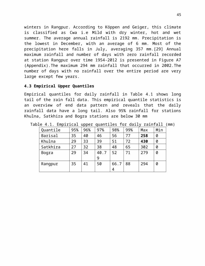
45

5.7 Bivariate Peaks over Threshold Methods

Bivariate peaks over threshold model are used to modal dependence between the daily rainfalls over a threshold. The scatter plots based on daily rainfall data represents approximate independence. Since there are almost 70% rainfall but there exist a correlation between stations above 95% thresholds (Figure 5.9).

20 40 60 80 100 120 140

2040

6080

120

Daily rainfall data with thresholds at 95% quantile

Barisal

Khu

lna

Figure 5.9. Scatter plot of daily rainfall data from Barisal and Khulna

The correlation between daily rainfall of two margins (stations) estimated by Kendall tau are very small and nearly zero. Because around 70% or more rainfall is zero for all stations .Estimated tau is large for stations Khulna and Satkhira compared to other.

For BGPD model the threshold are fixed at 95% quantile of daily rainfall data. Only parametric models (logistic and asymmetric logistic) are consider to model the dependence and the estimated strength of dependence between stations are nearly zero. The asymmetric parameters are also nearly 1. Hence the model reduced to logistic dependence model. We have also check dependences at different threshold between70 % to 95% but could not found any significance dependence between stations. In table 5.7 the summary of dependence estimates are presented.

46

Table 5.7.Summary of dependence between stations By BGPDStations Logistic Asymmetric logistic Kendall tau

(Daily rain)d d ψ1 ψ2

Barisal and Bogra 0.009 0.001 0.9959 0.9110 0.014Barisal and Khulna 0.001 0.001 0.9060 0.9995 0.001Barisal and Rangpur 0.0004 0.007 0.9013 0.999 -0.016Barisal and Satkhira 0.0013 0.0087 0.9998 0.8863 0.003Bogra and Khulna 0.0013 0.0012 0.9637 0.9105 0.027Bogra and Rangpur 0.001 0.012 0.8995 0.9993 0.004Bogra and Satkhira 0.0003 0.002 0.8950 0.9998 -0.004Khulna and Rangpur 0.001 0.003 0.861 0.999 0.0116Khulna and Satkhira 0.0003 0.002 0.9250 0.9609 0.0121Rangpur and Satkhira 0.004 0.004 0.9993 0.8498 -0.018

The quantile plots are presented in the following Figure 5.10.Only few rainfalls are above 98% and 99%

Figure 5.10 Quantile plots of BGPD at p=0.98 and 0.99 for logistic models.

47

5.8 Probability of Extreme Rainfall Estimation

In this section we will estimate some upper quantile probability from fitted BEVD model. Here bivariate logistic model as a parametric dependence function and non-parametric CFG and HT estimate of dependence are considered and the probability of upper tail region estimated only for 4 station that have significant upper tail dependence. The probability of extreme rainfall above 75% upper quantile for both stations is estimated by this formula P(X,Y)>75%. Figure 5.11 represents the annual maximum rainfall between station Barisal and Khulna.

P(X ,Y )>75 %=1−F (X )−G(Y )+G(X ,Y )

¿1−p (X<x )−p (Y < y )+ p¿)

Considering, X=rainfall at Barisal Y=rainfall at Khulna and x=75% quantile of Barisal and y=75% quantile of Barisal F (x)= margins of xand G( y )= margins ofy.

Figure 5.11.annual maximum

Estimated empirical probability are also estimated and presented in the following Table 5.8. The lowest probability of above 30% rainfall is 0.478 for stations Barisal and Khulna, and Bogra and Khulna. So the risk of annually maximum 30% rainfall in these areas is very large compared to other stations. The more important fact is that in station Barisal and Khulna the probability of having rainfall above 75% due to their dependence is also large .Hence these two stations are more vulnerable to natural hazards due to heavy rainfall. But the estimate of empirical probability is very low 0.86.

As well as Khulna and Satkhira, these two coastal regions have heavy rainfall due to dependence the joint probability approximately 0.13 whereas the empirical probability is 0.1.

But for all stations (Barisal and Khulna, Barisal and Satkhira, Khulna and Rangpur, and Khulna and Satkhira) the location is near the Bay of Bengal the joint probability of above 50% and even 75% above rainfall are little bit higher (0.29-0.34) compared to other stations.

50 100 150 200 250

100

200

300

400

yearly maximum rainfall

Barisal

Khu

lna

P(x,y)>(0.75)

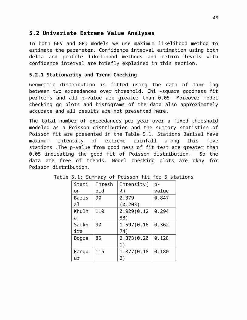
48

Table 5.9.Probability of extreme rainfall both stationsStations Tails log cfg HT emBarisal and Khulna 30% 0.478 0.481 0.485 0.5

50% 0.29 0.296 0.305 0.25975% 0.123 0.122 0.126 0.08695% 0.012 0.013 0.016 0.017

Barisal and Satkhira 30% 0.521 0.519 0.512 0.48350% 0.305 0.302 0.291 0.22475% 0.093 0.091 0.081 0.08695% 0.006 0.006 0.004 0

Khulna and Rangpur 30% 0.515 0.507 0.521 0.550% 0.302 0.291 0.311 0.27675% 0.093 0.085 0.103 0.10395% 0.013 0.011 0.016 0.017

Khulna and Satkhira 30% 0.51 0.512 0.519 0.48350% 0.338 0.344 0.354 0.27675% 0.119 0.123 0.133 0.10395% 0.013 0.014 0.019 0.017

The estimated probabilities from all extreme value distribution are approximately similar and large-r than empiric-al estimates. Thus we can rely on extreme value distribution for estimating risk of heavy rainfall.

49

Chapter 6Result Discussion and Conclusion

6.1 Discussion of Results

In modeling the statistical behavior of extreme rainfall recorded from five different stations over 58 years two approaches are used in this thesis. After checking trend and stationary rainfall the data are modeled as independent variable. In block maxima approach the generalized extreme value distribution is used to model annual maxima rainfall data .For peaks over threshold method generalized Pareto distribution is applied to model the daily rainfall data. The good fit of the model are confirmed by checking diagnostic plots. These two distributions are interrelated and provide similar inference about extreme values. Monte Carlo simulation also used to predict future return level when the no of exceedances are uncertain. Bootstrap confidence interval also estimated by using simulated data.

The next step is to model the dependence structure of extreme rainfall between two stations. For this purpose use BEVD and BGPD models are used with unit Fréchet margins. Both parametric and non-parametric dependence structure are applied to model BGEV. Bivariate logistic model a-and asymmetric models are used as parametric dependence function and nonparametric CFG and HT dependence estimator are used to estimate dependence. In modeling BGPD at 95% threshold based on daily rainfall data only parametric dependence structure are considered.

The performance of BEVD seems reasonable for estimating tail dependence between station .The dependence obtained from BEVD between Barisal and Khulna, Rangpur and Khulna and, Khulna and Stakhira are high .It seems realistic because the stations Barisal, Khulna and Satkhira are near Bay of Bengal and the geographic distance between margins are not far. Barisal lies in largest river the Ganges (Padma) .The tail dependence is almost zero for these stations Barisal and Rangpur, Bogra and Khulna and Rangpur Satkhira. It could be for their geographic distance.

Finally the some upper quantile probability is estimated to from BEVD models and compare with empirical probability. The estimated probability from BEVD is larger than empirical probability .So the risk of heavy rainfall estimation using these models are more adequate. These probability give the specific idea about the having extreme rainfall of this region. Estimated dependence between two stations from BGPD model are approximately zeros that indicating tail independence so only BEVD models are used in estimating the heavy rainfall.

According to the World Bank, Bangladesh ranks first at the list of increased risks of flooding, and second on the list of frequency and severity of storms in case climate changes further [30]. Bivariate extreme value model are useful in risk assessment of heavy rainfall at Bangladesh. This lends strong support to take proper caution against the natural disasters due to extreme rainfall and save the life and property.

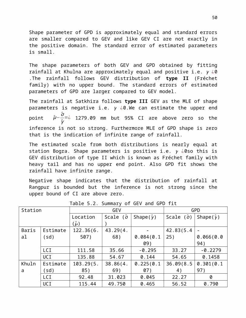
50

6.2 Further Scope :Modeling Zero Rainfall

The empirical probability of zero rainfall is estimated by proportion of days with no rainfall . The empirical probability is 0.7 which is very high for all five stations (Table 6.1).

Table 6.1 Probability of zero rainfall recorded from five stations Station Probability of zero rainfallBarisal 0.681Khulna 0.718Satkhira 0.716Bogra 0.711Rangpur 0.709

The minimum rainfall modeling via extreme value distribution is straightforward. But in our case all minimum rainfall are zero so it is tough to model the zero rainfall though extreme value distribution. Our further goal is to model minimum rainfall in extreme frame works and extends these study multivariate cases.

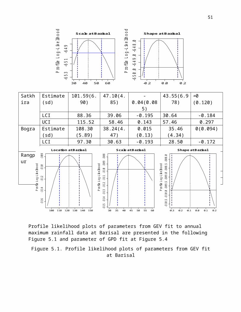
51

Appendix Notations used in this thesis

NotationsGEV Generalized Extreme value DistributionGPD Generalized Pareto DistributionPoT Peaks over ThresholdGoF Goodness of FitCI Confidence IntervalV VarianceCov Co-varianceD DevianceBVEVD Bivariate Extreme Value DistributionBGPD Bivariate Generalized Pareto DistributionCFG Capéraà Fougères-GenestHT Hall-Tajvidi estimate

M n Annual Maximumλ Intensityθ Extremal Indexμ Location parameter of GEVσ Scale parameter of GEV~σ Scale parameter of GPDγ Shape parameterZp Return levelsηu Probability of an individual observation

exceeding threshold uχ2 Goodness of fit test statisticsρ Pearson’s rhoτ Kendall tau⋁ Maximum∧ Minimum

A(t) Dependence functiond Strength of dependencer Dependence parameterψ1,ψ2 Asymmetric parameter

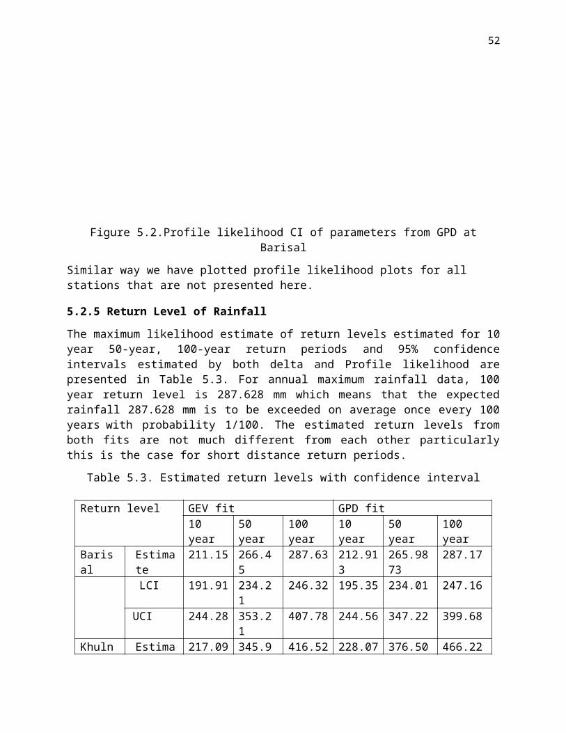
52

Delta method

The approximate confidence intervals of a large-sample maximum likelihood estimator

θ0=(θ1, θ2 ,….. θd)

with a variance-covariance matrix V(θ) where

V(θ) =[V (θ1 , θ2) ⋯ Cov (θ1 , θd)⋮ ⋱ ⋮

V (θd ,θ1) ⋯ V (θ1 ,θd)]

Suppose ϕ=h(θ) be a scaler function, then the MLE of ϕ0=h(θ0) and satisfies ϕ0∼N (ϕ0 ,V ϕ )

where V ϕ=∇ ϕTV θ∇ϕ with ∇ ϕ=[ δϕδ θ1

, δϕδ θ2

,………. , δϕδ θd

,]T

evaluated at θ0.

Profile Likelihood Method of CI

Numerical evaluation of profile likelihood method say for ,fixing μ=μ0 and then maximizing the log likelihood with respect to remaining parameters and repeat this process for some range of values μ0 .The 95% CI is obtained by re parameterization of GEV model considering zp as a model parameters and maximizing the log likelihood with respect to remaining parameters. The re parameterization can be done by following way

μ= zp+σγ [1− {−log (1−p ) }−γ ]

So the GEV model in terms of parameters (z p , σ , γ ¿ can be obtained by replacement of μ in eq (2.3) with (2.4). The plots of profile likelihood is usually make the certainty about the correctness of the resulting CI. Though the plots for a particular fit is tough but provide better accuracy particularly long return period. The horizontal line of figure (1) is at maximum profile likelihood value minus the 0.975 quantile of χ1

2 distribution function. Therefore all the return levels associated profile likelihood above the lower horizontal line in the figure are between 95% Confidence region and the values below the line are outside of 95% region. Approximate CI is the points that cross the horizontal line and the blue vertical line is the estimated CL and middle black line is MLE.

250 300 350 400

-318

-314

-310

100 year

Pro

file

Log-

Like

lihoo

d

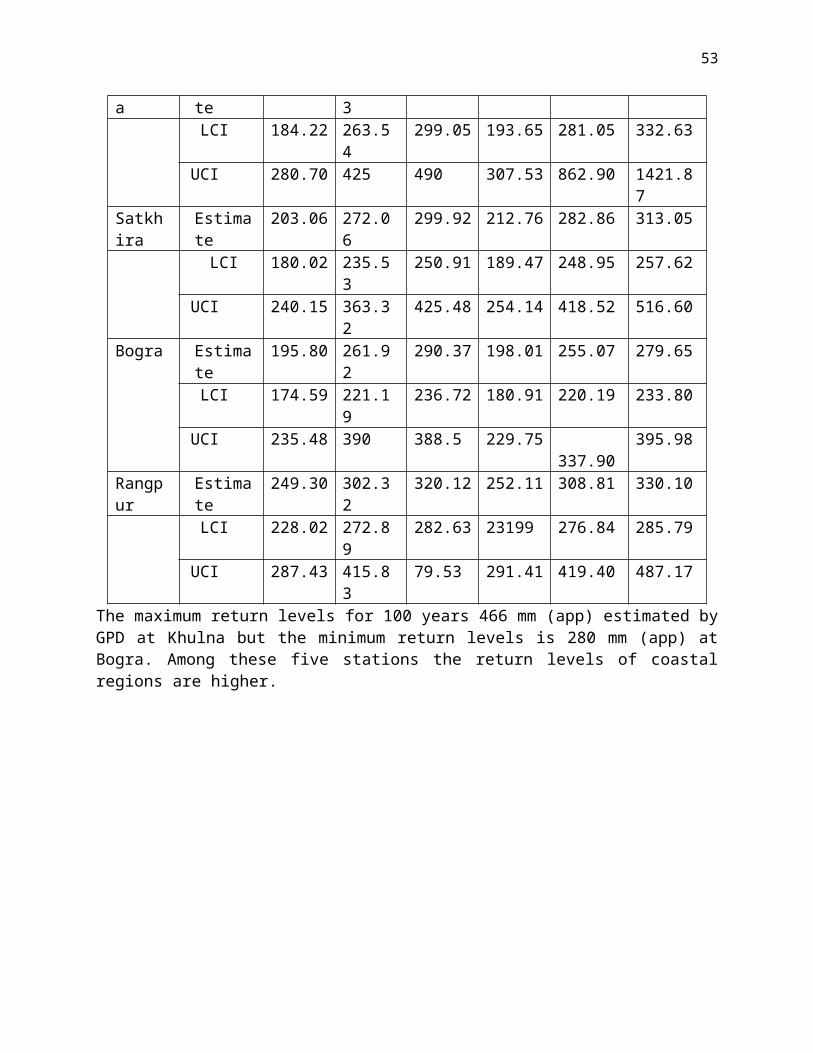
53

Figure A1.Profile likelihood CI of 100 years return levels at Barisal

Mean residual plots

Mean residual plots based on the mean of GPD and the mean is

E [ X ]={~σ

1−γ, γ<1∧γ ≠0~σ γ=0

The validity of threshold u0 for GPD refers any u0<u subject to appropriate change of scale parameters ~σ . The estimate of mean excess of threshold change approximately linearly with u for all u0<u . It can be written from definition of GPD

E ¿

If we plot the data points

{(u , 1nu∑i=1

nu

(x ( i)−u )) :u<xmax}

Where x (1 ) , x (2) ,……x (nu) are the nuobservations that exceed u and the resulting plots are known as mean residual plots that are approximately linear aboveu0. Based on the approximate normality of sample mean the 95% CI also added to the plot.

Figure A2.Mean residual plot of daily rainfall data at Barisal

0 50 100 150 200

1020

3040

5060

Mean residual life plot for Rain fall data at Barisal

Threshold

Mea

n E

xces

s

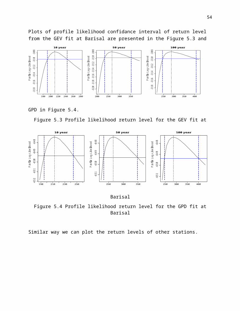
54

Threshold range plot

This method is mainly based on estimation of model at several ranges of thresholds. The asymptotic motivation for the GPD is valid above level u0 and the estimates of shape parameters should be identical and estimates of scale should n be linear in u. σ u denoted as a scale corresponding the threshold u ,then the following relation holds for u0<u

σ u=σu0+γ (u−u0 )

In order to avoid the difficulties due to γ=0reparameterize σ u by the following way

σ ¿=σu−γu

This leads σ ¿ as a constant for all u0<u.Ploting both σ ¿ ¿ γ versus u with CI, the lowest value of u for which the estimates are nearly constant is selected as a threshold.

Figure A3.Threshold range plot at Barisal

Station Khulna

Yearly rainfall at Khulna

Year

Rai

nfal

l

1960 1970 1980 1990 2000 2010

100

200

300

400 zero rainfall

max rainfall

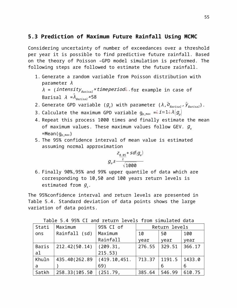
55

Figure A4.Annual maximum rainfall and number of zero rainfall per year over 1954-2012

Station Satkhira

Figure A5 Annual maximum rainfall and number of zero rainfall per year over 1954-2012

Station Bogra

Figure A5. Annual maximum rainfall and number of zero rainfall per year over 1954-2012

Station Rangpur

Yearly rainfall at Satkhira

Year

Rai

nfal

l

1960 1970 1980 1990 2000 2010

100

200

300

400

zero rainfallmax rainfall

Yearly rainfall at Rangpur

Year

Rai

nfal

l

1960 1970 1980 1990 2000 2010

5015

025

035

0

zero rainfallmax rainfall

Yearly rainfall at Bogra

Year

Rai

nfal

l

1960 1970 1980 1990 2000 2010

100

200

300

400

500

zero rainfallmax rainfall

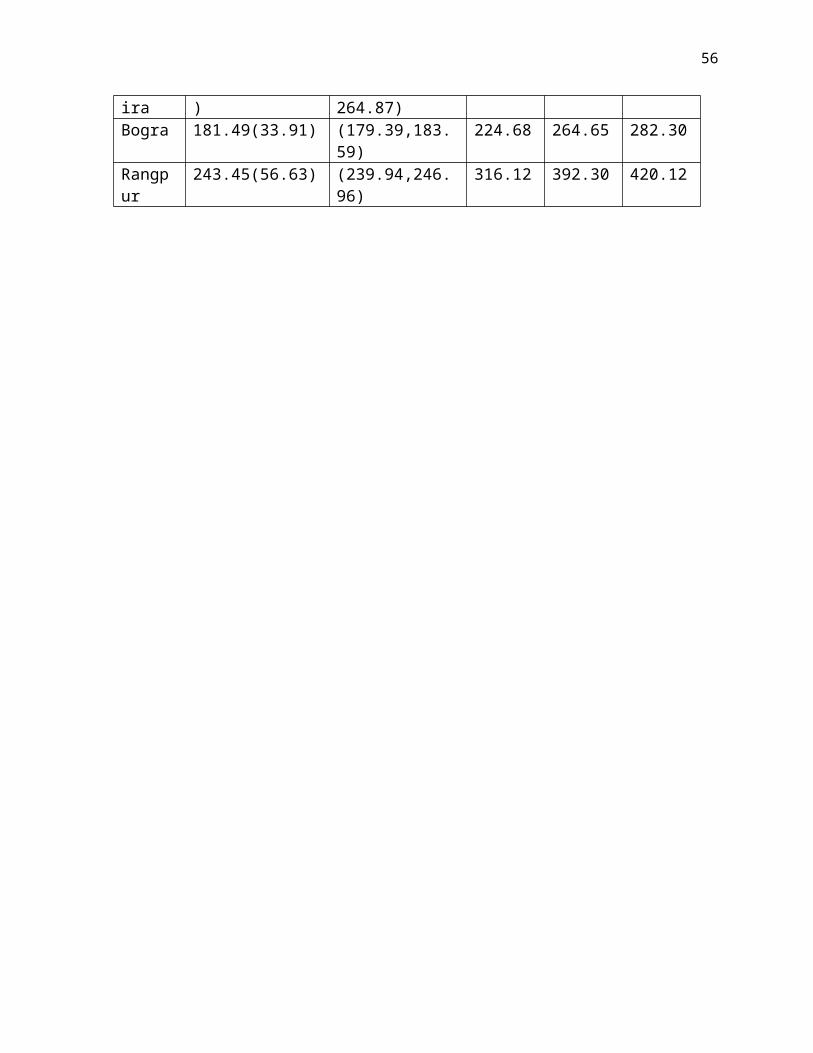
56

Figure A6.Annual maximum rainfall and number of zero rainfall per year over 1954-2012

References 1. Murshed, S. B., Islam, A. K. M., & Khan, M. S. A. (2011, January). Impact of climate

change on rainfall intensity in Bangladesh. In 3rdInternationalConferenceonWaterandFloodManagement,ICWFM.

2. Mahmood, S. A. I. (2012). Impact of Climate Change in Bangladesh: The Role of Public Administration and Government’s Integrity. Journal of Ecology and the NaturalEnvironment, 4(8), 223-240.

3. Field, C. B., Barros, V. R., Dokken, D. J., Mach, K. J., Mastrandrea, M. D., Bilir, T. E., ... & White, L. L. (2014). IPCC, 2014, Climate Change 2014: Impacts, Adaptation, and Vulnerability. Part A: Global and Sectoral Aspects. Contribution of Working Group II to the Fifth Assessment Report of the Intergovernmental Panel on Climate Change Cambridge University Press, Cambridge, United Kingdom and New York, NY, USA, 1132 pp.

4. Barros, V.R., C.B. Field, D.J. Dokken, M.D. Mastrandrea, K.J. Mach, T.E. Bilir, M. Chatterjee, K.L. Ebi, Y.O. Estrada, R.C. Genova, B. Girma, E.S. Kissel, A.N. Levy, S. MacCracken, P.R. Mastrandrea, and L.L. White ,(2014),IPCC, 2014: Climate Change 2014: Impacts, Adaptation, and Vulnerability. Part B: Regional Aspects. Contribution of Working Group II to the Fifth Assessment Report of the Intergovernmental Panel on Climate Change, Cambridge University Press, Cambridge, United Kingdom and New York, NY, USA, 688 pp.

5. Parry, M. L. (Ed.). (2007). Climate Change 2007: impacts, adaptation and vulnerability: contribution of Working Group II to the fourth assessment report of the Intergovernmental Panel on Climate Change (Vol. 4). CambridgeUniversityPress

6. Mirza, M. Q., Warrick, R. A., Ericksen, N. J., & Kenny, G. J. (1998). Trends and persistence in precipitation in the Ganges, Brahmaputra and Meghna river basins. HydrologicalSciencesJournal, 43(6), 845-858.

7. Wasimi, S. A. (2009). Climate change trends in Bangladesh. In Proc. of 2ndInternational.

8. Allan, R. P., & Soden, B. J. (2008). Atmospheric warming and the amplification of precipitation extremes. Science, 321(5895), 1481-1484.

9. Fung, C. F., Farquharson, F., & Chowdhury, J. (2006). 4 HYDRO-CLIMATOLOGY-Climate change and impacts of climate change-Exploring the impacts of climate change on water resources--Regional impacts at a regional scale: Bangladesh. IAHSPublications-SeriesofProceedingsandReports, 308, 389-393

10. Senior, C. A., Jones, R. G., Lowe, J. A., Durman, C. F., & Hudson, D. (2002). Predictions of extreme precipitation and sea–level rise under climate change. PhilosophicalTransactionsoftheRoyalSocietyofLondonA:Mathematical,PhysicalandEngineeringSciences, 360(1796), 1301-1311.

11. Christensen, J. H., Hewitson, B., Busuioc, A., Chen, A., Gao, X., Held, R.,& Dethloff, K. (2007). Regional climate projections. ClimateChange,2007:ThePhysicalScienceBasis.Contribution of Working group I to the Fourth Assessment Report of theIntergovernmentalPanelonClimateChange,UniversityPress,Cambridge,Chapter11, 847-940.

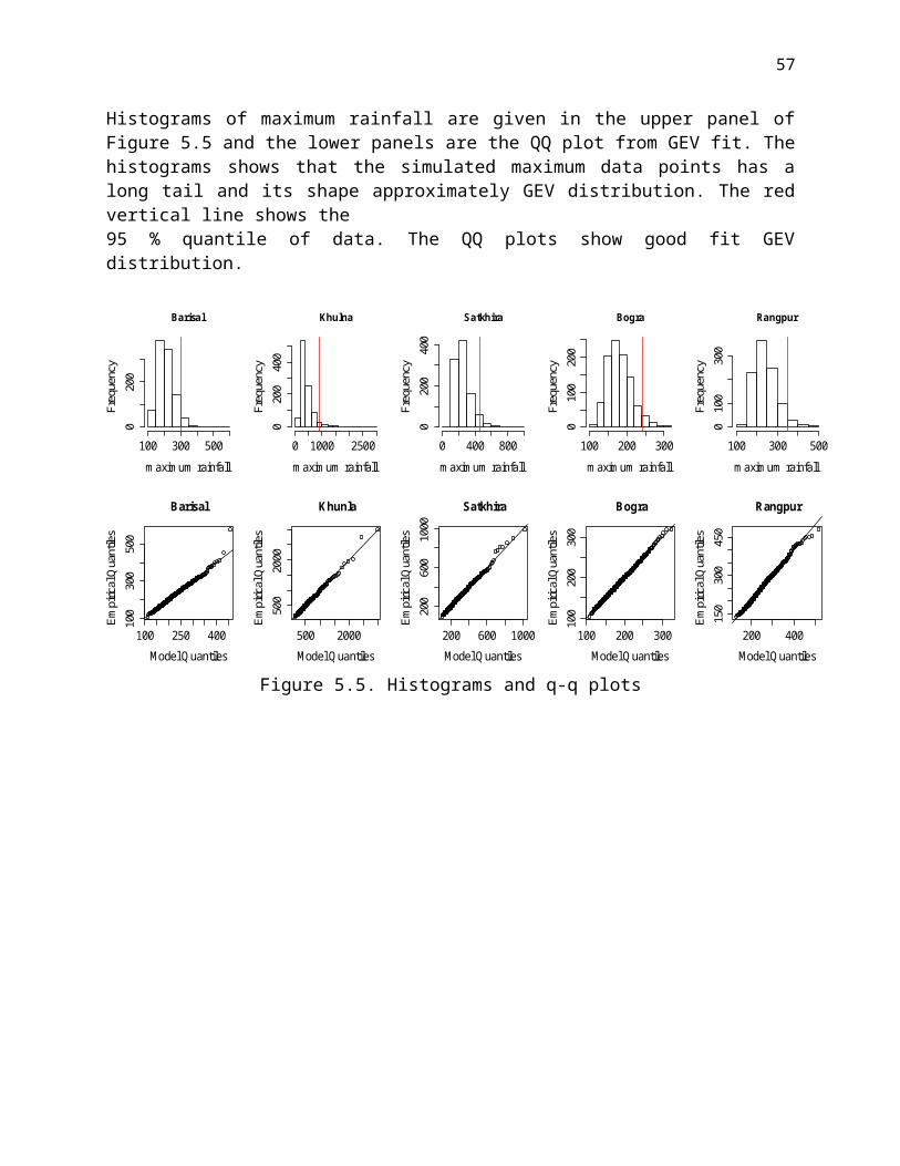
57

12. National Plan for Disaster Management,(2010), DisasterManagementBureau13. Shahid, S. (2011). Trends in extreme rainfall events of Bangladesh. Theoretical and

appliedclimatology, 104(3-4), 489-499.14. Daily Star (2011). Climate change: Threat to international peace and security. Available

at: http://www.thedailystar.net/newDesign/newsdetails.php?nid=198040. Accessed on August 11, 2011.

15. New Age (2011). River bank erosion, displacement and consequences. Available at: http://newagebd.com/newspaper1/op-ed/33554.html. Accessed September 19, 2011.

16. Rootzén, H., & Tajvidi, N. (2006). Multivariate generalized Pareto distributions.Bernoulli, 917-930.

17. Cooley, D. S. (2005). Statisticalanalysisofextremesmotivatedbyweatherandclimatestudies:appliedandtheoreticaladvances (Doctoral dissertation, University of Colorado).

18. Tawn, J. A. (1988). Bivariate extreme value theory: models and estimation. Biometrika, 75(3), 397-415.

19. Joe, H. (1997). Multivariatemodelsandmultivariatedependenceconcepts. CRC Press.20. Ferreira, H. (2014). Bivariate tail dependence and the generation of Multivariate Extreme

Value distributions. Communications in Statistics-Theory and Methods, 43(24), 5318-5325.

21. Coles, S., Bawa, J., Trenner, L., & Dorazio, P. (2001). Anintroduction to statisticalmodelingofextremevalues (Vol. 208). London: Springer.

22. Finkenstadt, B., & Rootzén, H. (Eds.). (2003). Extreme values in finance,telecommunications,andtheenvironment. CRC Press.

23. Smith, R. L., Tawn, J. A., & Coles, S. G. (1997). Markov chain models for threshold exceedances. Biometrika, 84(2), 249-268.

24. Olivares, M .A & Forero, G, C,(2010).Goodness-of-Fit Testing. InternationalEncyclopediaofEducation.7, pp. 190-196.

25. Wikipedia 26. Beirlant, J., Goegebeur, Y., Segers, J., & Teugels, J. (2006). Statisticsofextremes:theory

andapplications. John Wiley & Sons. 27. Rakonczai, P. (2012). Multivariate Threshold Models with Applications to Wind Speed

Data. 28. Rakonczaia, P., & Tajvidia, N. (2010). On prediction of bivariate extremes.29. en.climate-data.org 30. Groen,T,E & Jacobs ,C.(2012).Risk Mapping Bangladesh Sector Disaster Risk Reduction

& Emergency Aid. ActionAid, Bangladesh.