Dalle Molle Institute for Artificial Intelligence (IDSIA)

Lugano, Switzerland (www.idsia.ch)

LSTM Hybrid Recurrent Neural

Networks in Music and Speech

Douglas Eck

Thanks To

• Juergen Schmidhuber

• Felix Gers

• Alex Graves

Overview

• Research background

• Motivation for choosing RNNs for music and speech

• Identification of RNN shortcomings

• Introduction to hybrid RNN “Long Short-Term Memory” (LSTM)

• Two Applications of LSTM– Music Composition

– Speech Recognition

Goals

• Unified theory of human cognition and machine learning

• Constraints come from, e.g, human performance, neurobiology and learning theory

• Focus on audition: speech and music

• Want to (temporarily) increase error

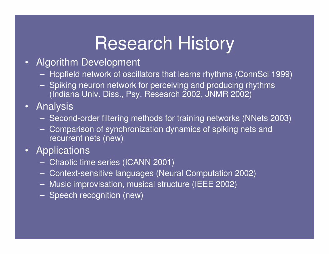
Research History• Algorithm Development

– Hopfield network of oscillators that learns rhythms (ConnSci 1999)

– Spiking neuron network for perceiving and producing rhythms (Indiana Univ. Diss., Psy. Research 2002, JNMR 2002)

• Analysis– Second-order filtering methods for training networks (NNets 2003)

– Comparison of synchronization dynamics of spiking nets and recurrent nets (new)

• Applications – Chaotic time series (ICANN 2001)

– Context-sensitive languages (Neural Computation 2002)

– Music improvisation, musical structure (IEEE 2002)

– Speech recognition (new)

Speech and Music Prediction

• Listeners attend to certain kinds of temporal

structure (e.g. metrical structure, speech rhythm)

• Invariance across other structure (e.g. tempo

and acceleration in music; speaker rate)

• Music and speech are both hierarchical with

recognizable atomic units (e.g. notes, phones)

• A set of inductive biases for music and speech

related to long time-scale structure

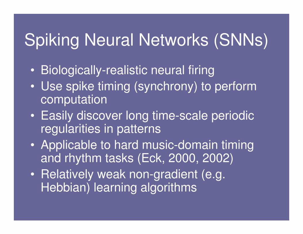
Spiking Neural Networks (SNNs)

• Biologically-realistic neural firing

• Use spike timing (synchrony) to perform computation

• Easily discover long time-scale periodic regularities in patterns

• Applicable to hard music-domain timing and rhythm tasks (Eck, 2000, 2002)

• Relatively weak non-gradient (e.g. Hebbian) learning algorithms

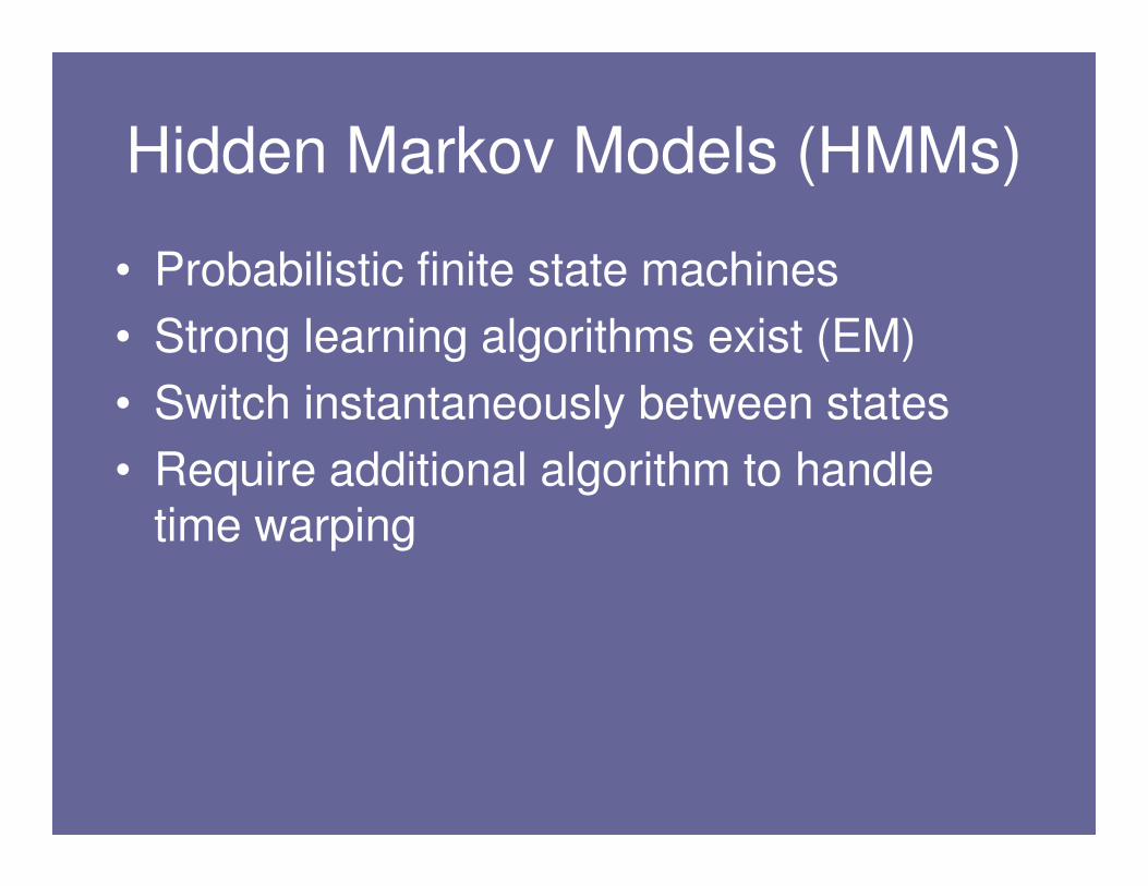
Hidden Markov Models (HMMs)

• Probabilistic finite state machines

• Strong learning algorithms exist (EM)

• Switch instantaneously between states

• Require additional algorithm to handle time warping

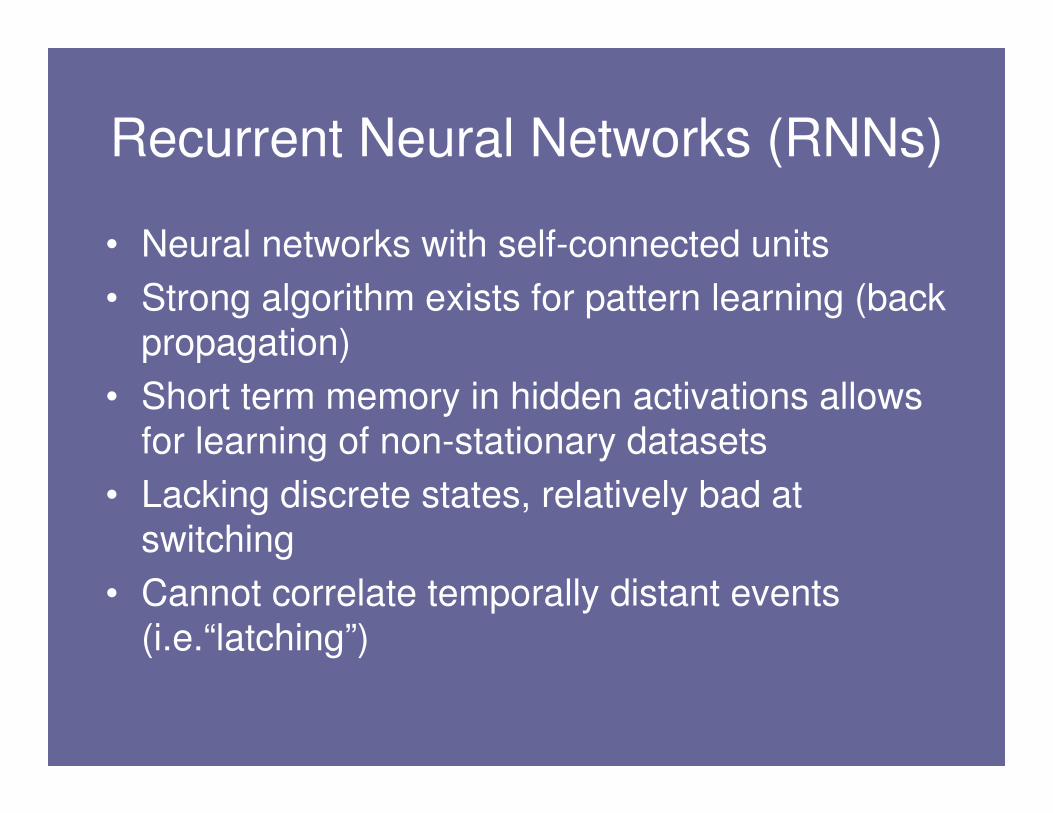
Recurrent Neural Networks (RNNs)

• Neural networks with self-connected units

• Strong algorithm exists for pattern learning (back

propagation)

• Short term memory in hidden activations allows

for learning of non-stationary datasets

• Lacking discrete states, relatively bad at

switching

• Cannot correlate temporally distant events

(i.e.“latching”)

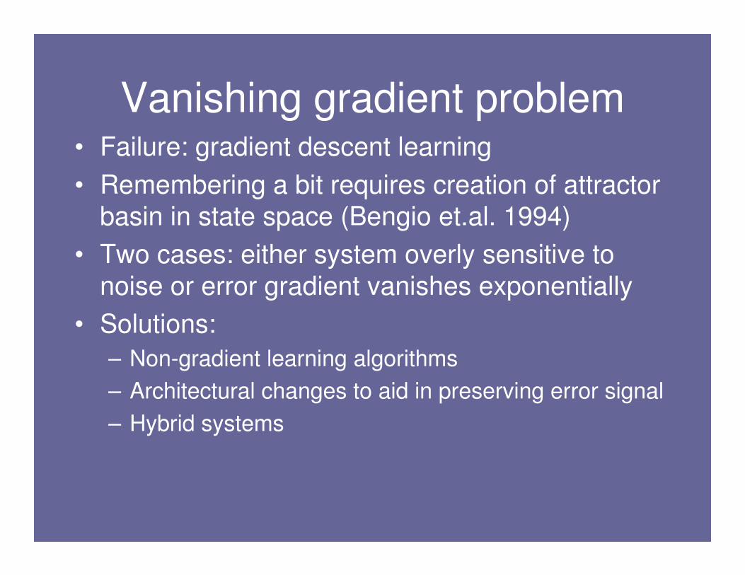
Vanishing gradient problem• Failure: gradient descent learning

• Remembering a bit requires creation of attractor

basin in state space (Bengio et.al. 1994)

• Two cases: either system overly sensitive to

noise or error gradient vanishes exponentially

• Solutions:

– Non-gradient learning algorithms

– Architectural changes to aid in preserving error signal

– Hybrid systems

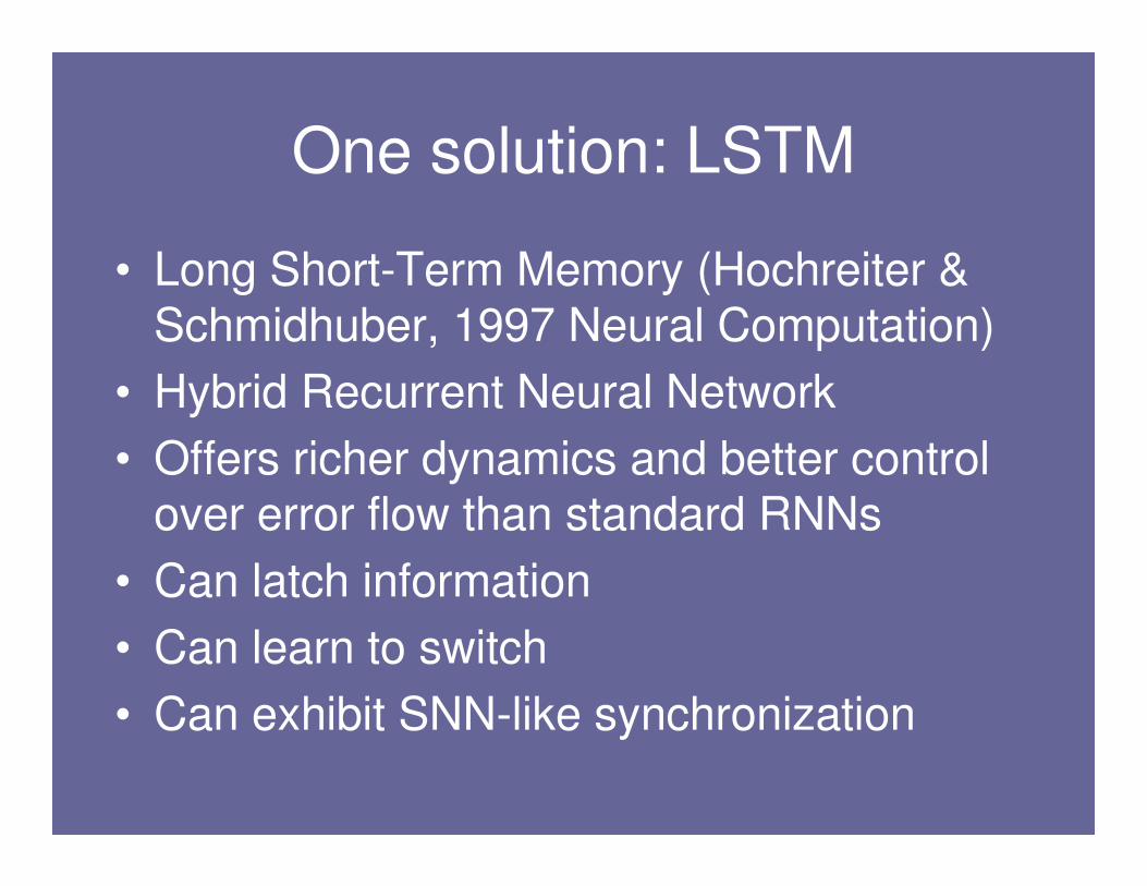
One solution: LSTM

• Long Short-Term Memory (Hochreiter & Schmidhuber, 1997 Neural Computation)

• Hybrid Recurrent Neural Network

• Offers richer dynamics and better control over error flow than standard RNNs

• Can latch information

• Can learn to switch

• Can exhibit SNN-like synchronization

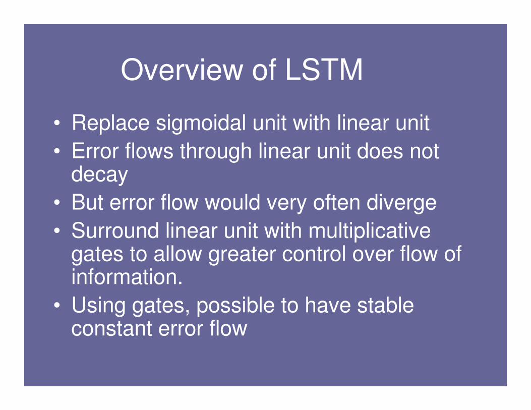
Overview of LSTM

• Replace sigmoidal unit with linear unit

• Error flows through linear unit does not decay

• But error flow would very often diverge

• Surround linear unit with multiplicative gates to allow greater control over flow of information.

• Using gates, possible to have stable constant error flow

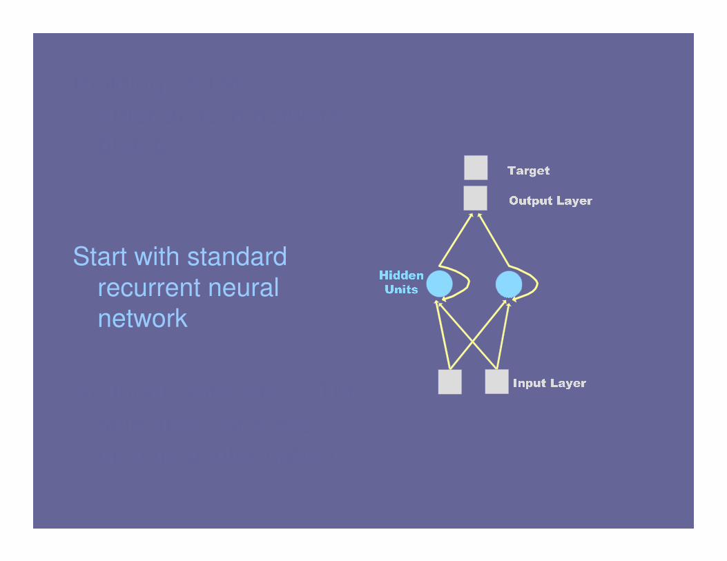
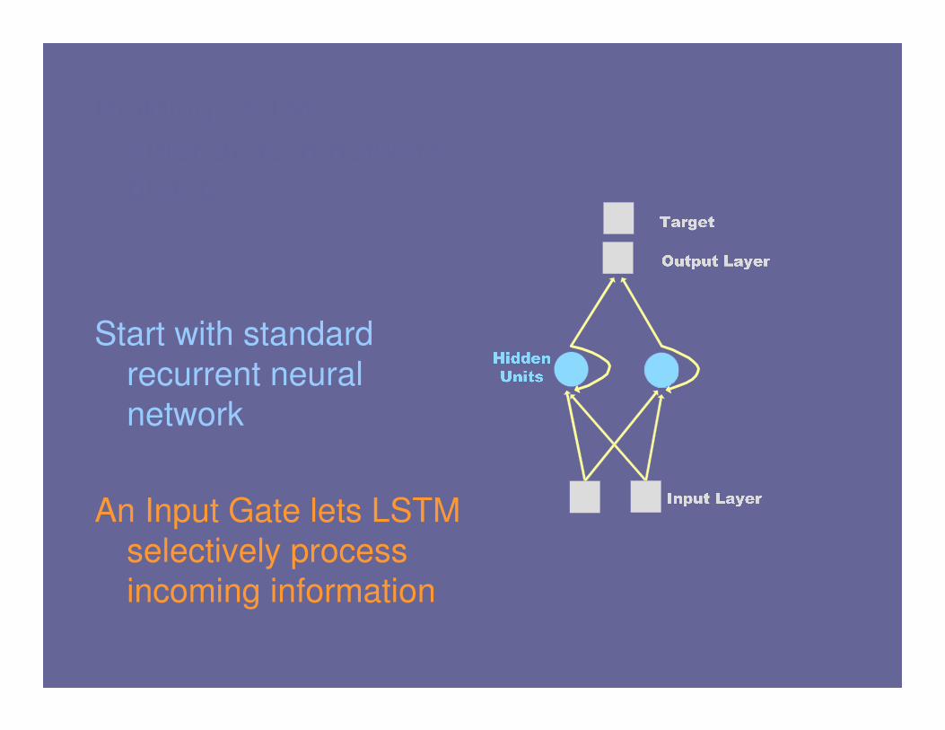
Building LSTM...

other units in network

blah b

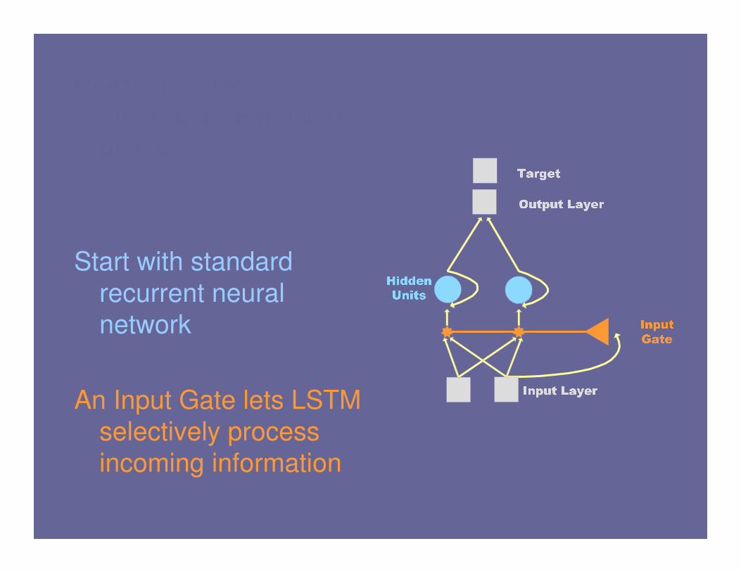
Start with standard

recurrent neural

network

An Input Gate lets LSTM

selectively process

incoming information

Building LSTM...

other units in network

blah b

Start with standard

recurrent neural

network

An Input Gate lets LSTM

selectively process

incoming information

Building LSTM...

other units in network

blah b

Start with standard

recurrent neural

network

An Input Gate lets LSTM

selectively process

incoming information

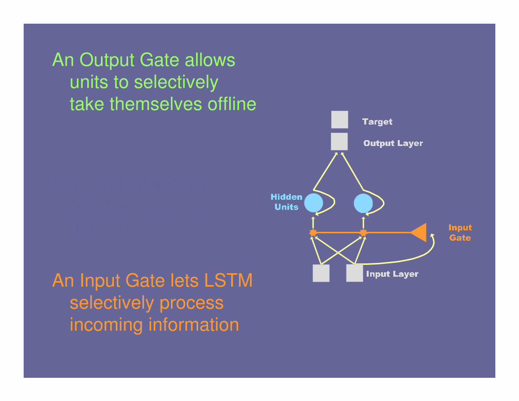
An Output Gate allows

units to selectively

take themselves offline

Start with standard

recurrent neural

network

An Input Gate lets LSTM

selectively process

incoming information

An Output Gate allows

units to selectively

take themselves offline

Forget Gate enables a

block to empty its own

memory contents

An Input Gate lets LSTM

selectively process

incoming information

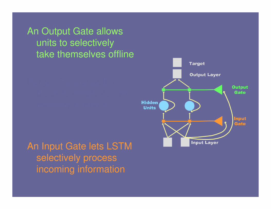
An Output Gate allows

units to selectively

take themselves offline

A Forget Gate enables

units to empty their

own memory contents

An Input Gate lets LSTM

selectively process

incoming information

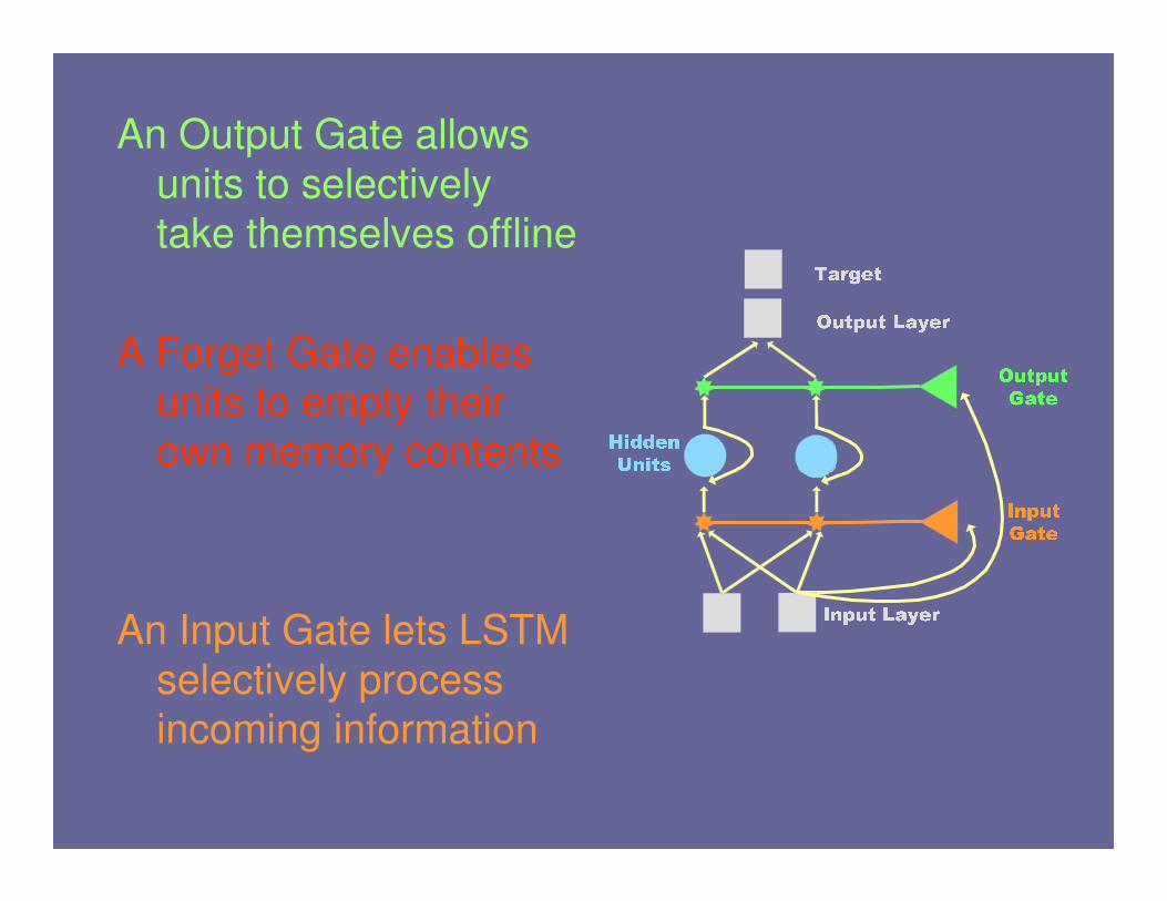
An Output Gate allows

units to selectively

take themselves offline

A Forget Gate enables

units to empty their

own memory contents

An Input Gate lets LSTM

selectively process

incoming information

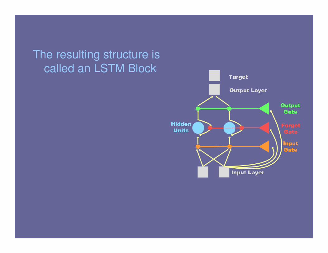
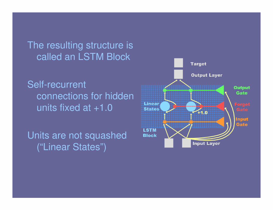
The resulting structure is

called an LSTM Block

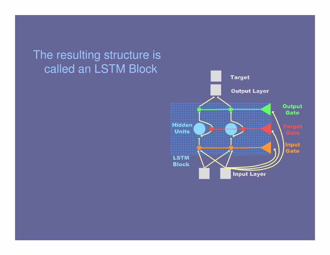
The resulting structure is

called an LSTM Block

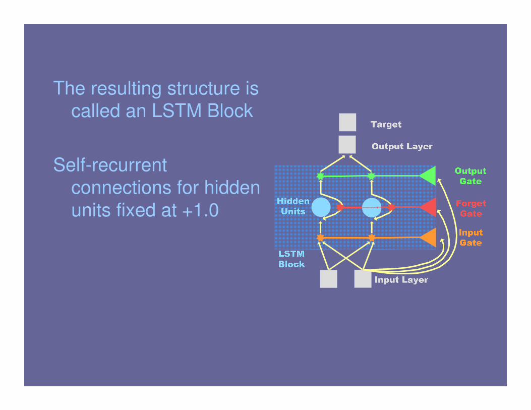
The resulting structure is

called an LSTM Block

Self-recurrent

connections for hidden

units fixed at +1.0

The resulting structure is

called an LSTM Block

Self-recurrent

connections for hidden

units fixed at +1.0

The resulting structure is

called an LSTM Block

Self-recurrent

connections for hidden

units fixed at +1.0

Units are not squashed

(“Linear States”)

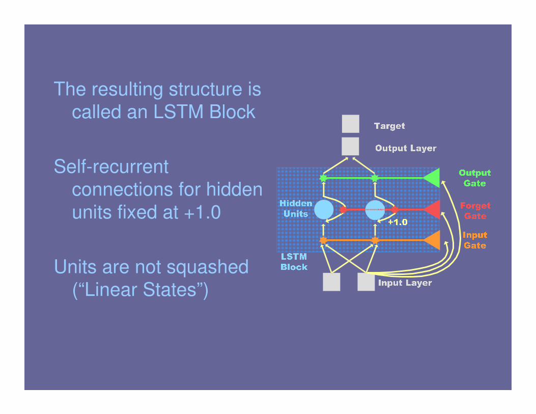
The resulting structure is

called an LSTM Block

Self-recurrent

connections for hidden

units fixed at +1.0

Units are not squashed

(“Linear States”)

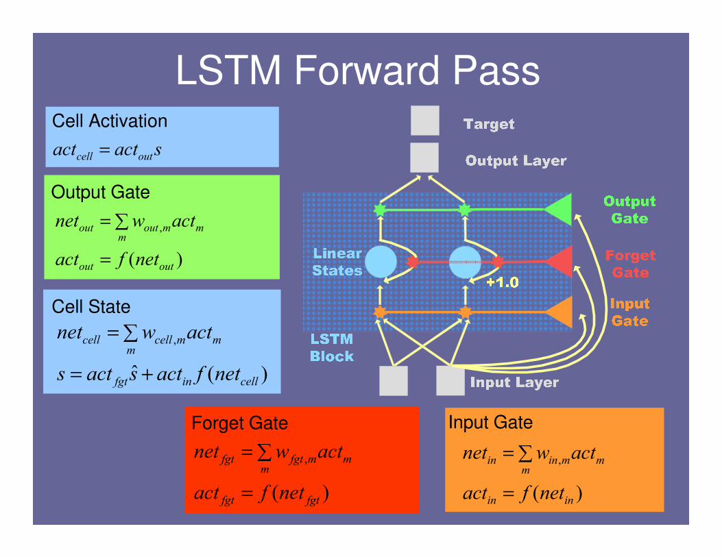
Input Gate

)(

,

inin

mm

minin

netfact

actwnet

=

∑=

LSTM Forward Pass

)(ˆ

,

cellinfgt

mm

mcellcell

netfactsacts

actwnet

+=

∑=

Cell State

sactact outcell =

Cell Activation

)(

,

fgtfgt

mm

mfgtfgt

netfact

actwnet

=

∑=

Forget Gate

)(

,

outout

mm

moutout

netfact

actwnet

=

∑=

Output Gate

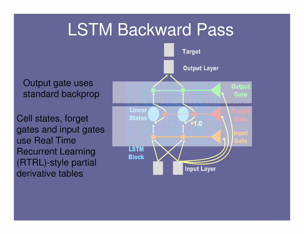
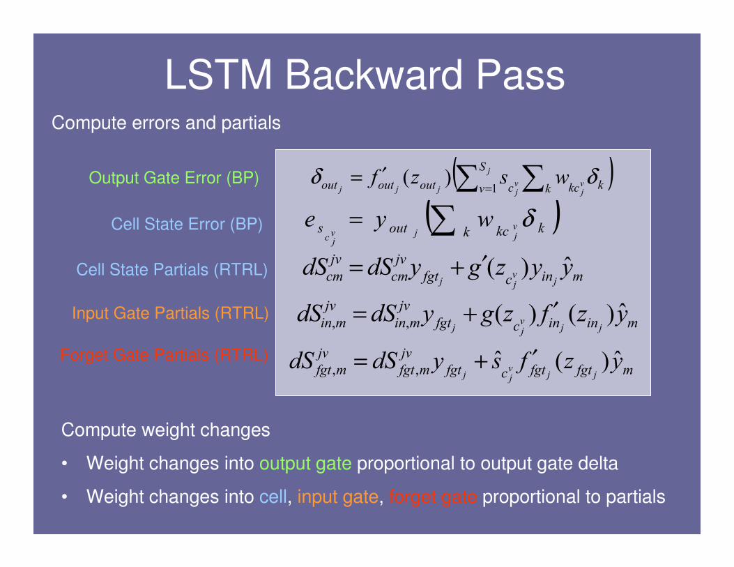
LSTM Backward Pass

Output gate uses standard backprop

Cell states, forget gates and input gates

use Real Time Recurrent Learning

(RTRL)-style partial

derivative tables

Connectivity

• Recurrent connections

back into gates and cells very useful

• Additional feed-forward layers are useful

• Additional LSTM layers

probably not useful: gradient truncated

Known Limitations• Difficult to train

– High nonlinearity in gates

– Kalman filtering helps (Perez, Gers, Schmidhuber & Eck 2003)

– Currently exploring other 2nd order approaches• natural gradient (Amari)

• stochastic meta-descent (SMD, Schraudholph)

• High sensitivity to initial conditions – Gates must self-configure at least partially before

error can flow

• Failure on e.g. Mackey-Glass time delay chaotic time series (Gers, Eck and Schmidhuber, 2001)

Experiment: Music Composition• Task: perform next-note composition

• RNN outperforms 3rd order transition tables (Mozer 1996)

• RNN does not learn global musical structure when trained on popular waltzes

• Mozer: “While the local contours made sense, the pieces were not musically coherent, lacking thematic structure and having minimal phrase structure and rhythmic organization”.

LSTM Music Composer• Goal: Learn high-level musical structure

and use that structure to support music composition

• Experiment: Small 12-bar blues dataset with simple melodies

• Results: When composing, did use chord structure to constrain melody choices

• Led to effect of freer improvisation followed by close reproduction of training melodies

Speech Recognition

• NNs already show promise (Boulard, Robinson, Bengio)

• LSTM may offer a better solution by finding long-timescale structure in speech

• At least two areas where this may help:

– Time warping (rate invariance)

– Dynamic, learned model of phoneme

segmentation (with little apriori knowledge)

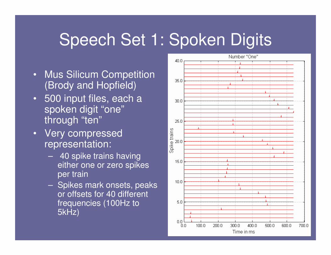
Speech Set 1: Spoken Digits

• Mus Silicum Competition (Brody and Hopfield)

• 500 input files, each a spoken digit “one”through “ten”

• Very compressed representation:– 40 spike trains having

either one or zero spikes per train

– Spikes mark onsets, peaks or offsets for 40 different frequencies (100Hz to 5kHz)

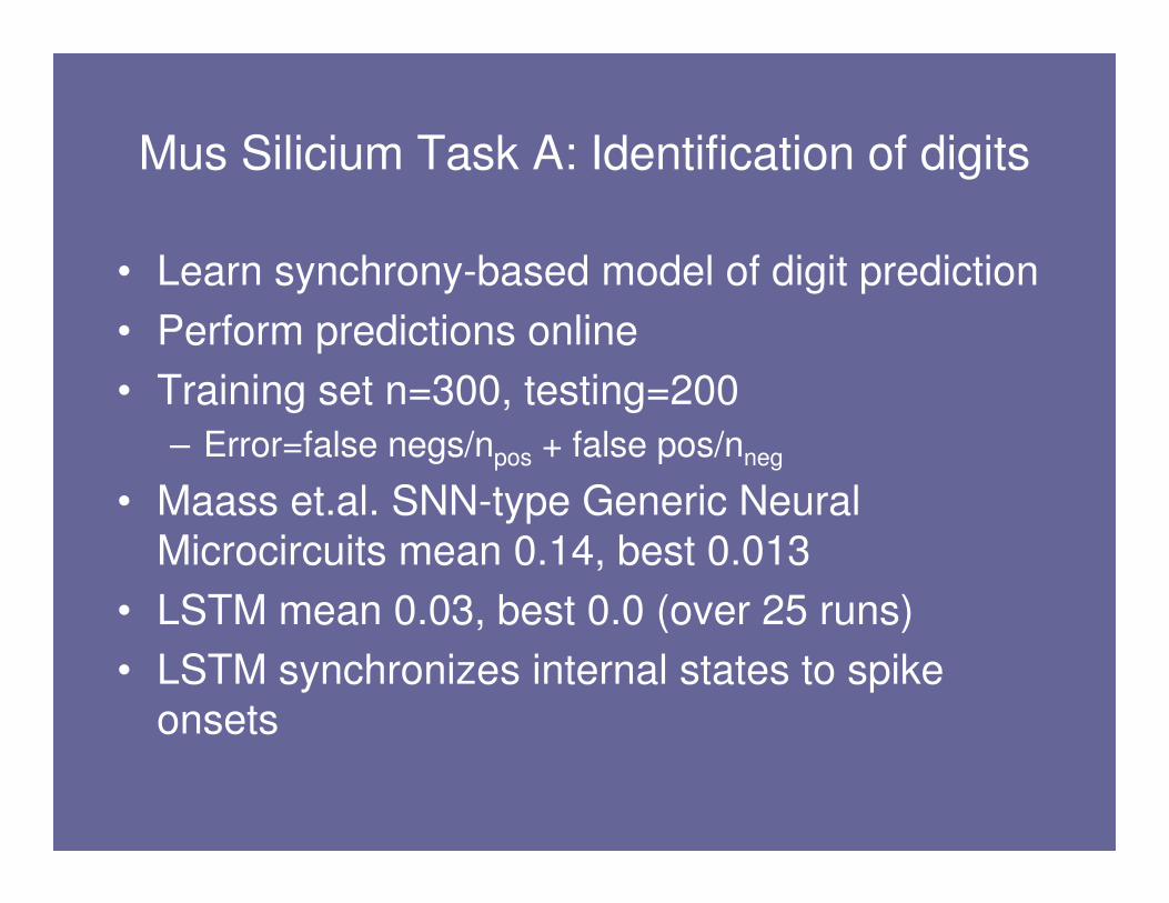
Mus Silicium Task A: Identification of digits

• Learn synchrony-based model of digit prediction

• Perform predictions online

• Training set n=300, testing=200

– Error=false negs/npos + false pos/nneg

• Maass et.al. SNN-type Generic Neural

Microcircuits mean 0.14, best 0.013

• LSTM mean 0.03, best 0.0 (over 25 runs)

• LSTM synchronizes internal states to spike

onsets

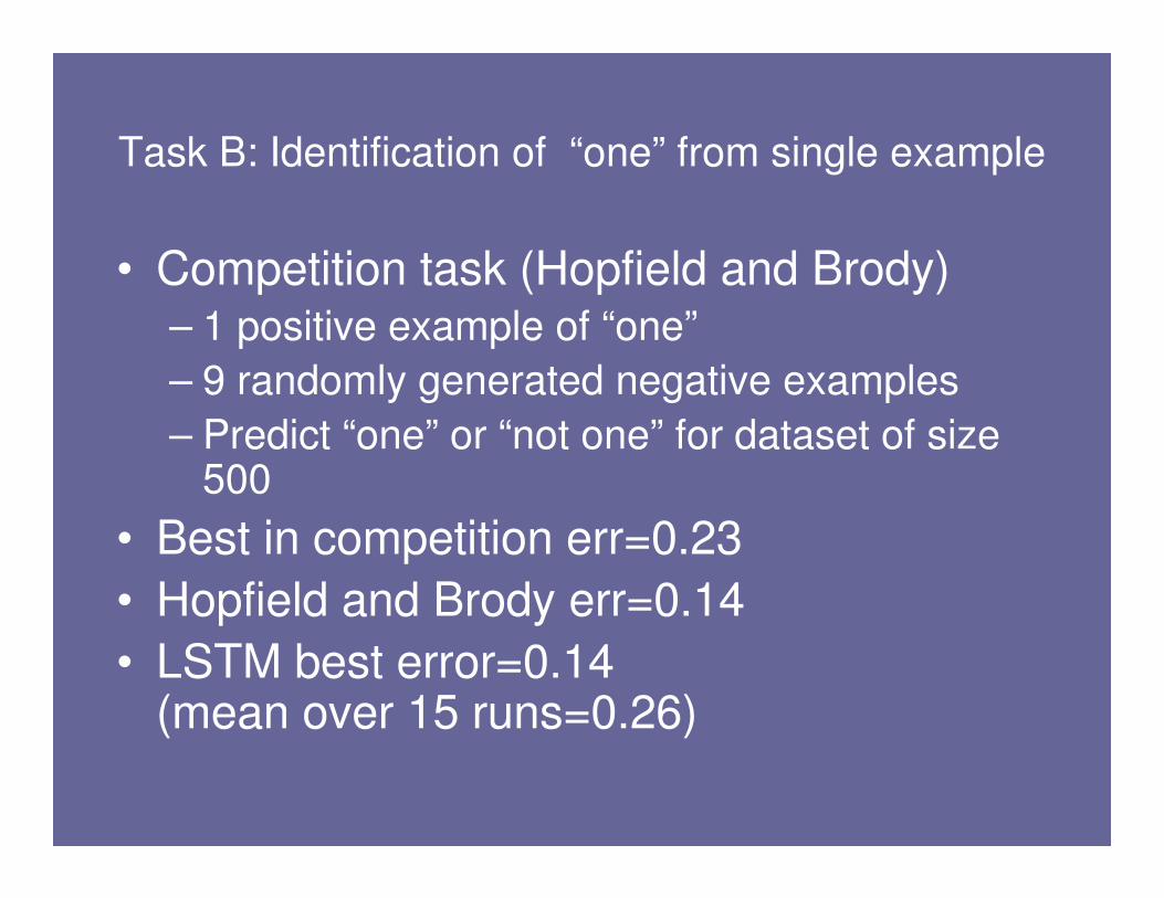
Task B: Identification of “one” from single example

• Competition task (Hopfield and Brody)– 1 positive example of “one”

– 9 randomly generated negative examples

– Predict “one” or “not one” for dataset of size 500

• Best in competition err=0.23

• Hopfield and Brody err=0.14

• LSTM best error=0.14 (mean over 15 runs=0.26)

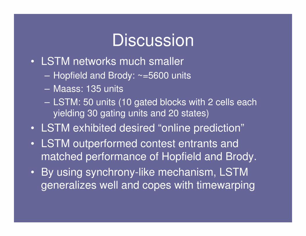
Discussion• LSTM networks much smaller

– Hopfield and Brody: ~=5600 units

– Maass: 135 units

– LSTM: 50 units (10 gated blocks with 2 cells each yielding 30 gating units and 20 states)

• LSTM exhibited desired “online prediction”

• LSTM outperformed contest entrants and

matched performance of Hopfield and Brody.

• By using synchrony-like mechanism, LSTM

generalizes well and copes with timewarping

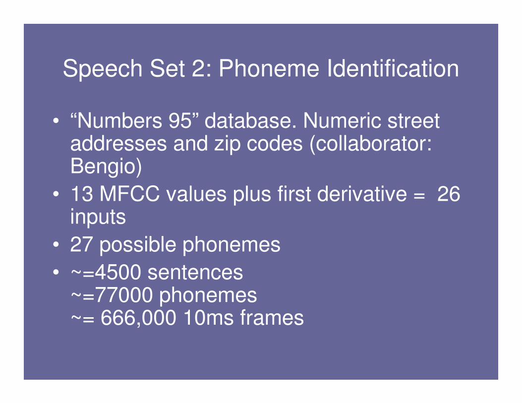
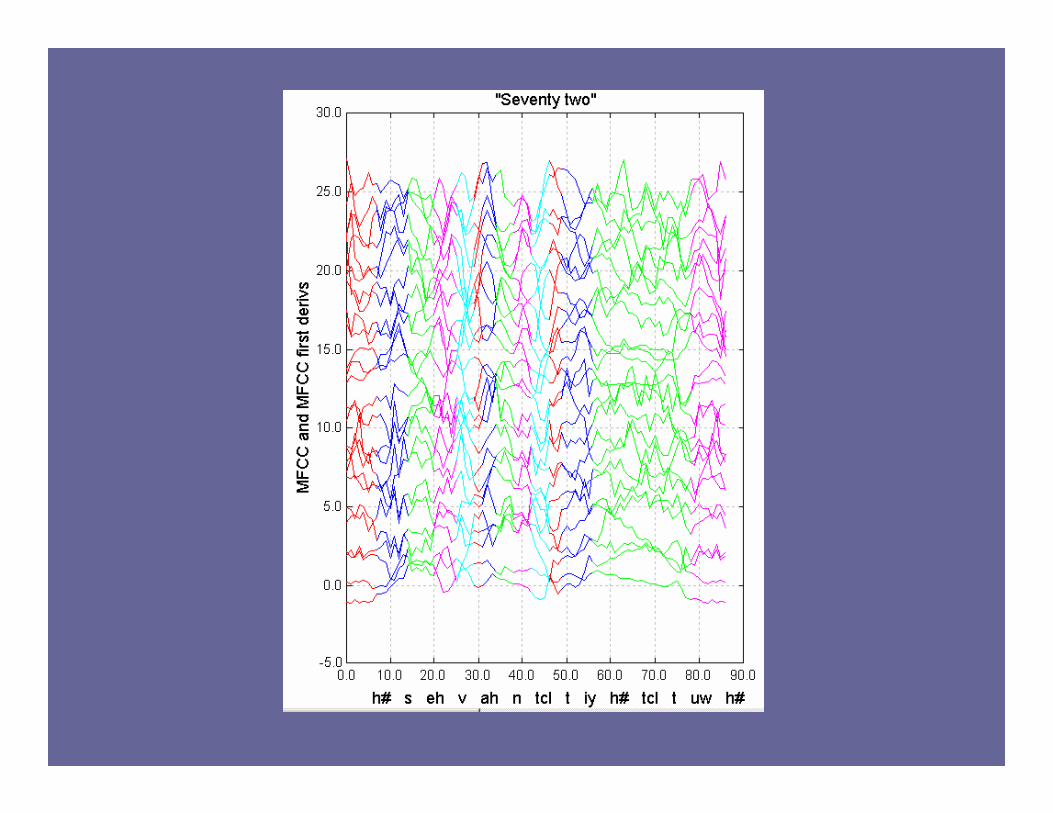
Speech Set 2: Phoneme Identification

• “Numbers 95” database. Numeric street addresses and zip codes (collaborator: Bengio)

• 13 MFCC values plus first derivative = 26 inputs

• 27 possible phonemes

• ~=4500 sentences~=77000 phonemes~= 666,000 10ms frames

Task A: Single phoneme identification

• Categorize phonemes in isolation.

• Prediction made only at last time step

• LSTM has no advantage because no history

• Benchmark ~=92% correct (S. Bengio)

• LSTM ~= 85%*

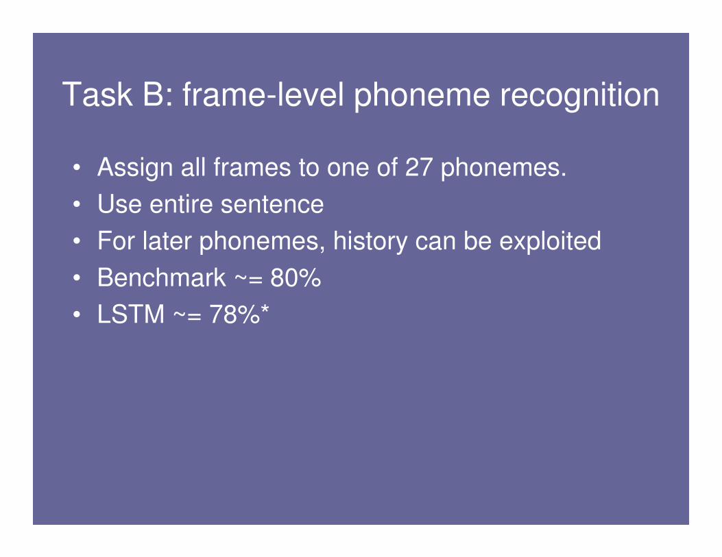
Task B: frame-level phoneme recognition

• Assign all frames to one of 27 phonemes.

• Use entire sentence

• For later phonemes, history can be exploited

• Benchmark ~= 80%

• LSTM ~= 78%*

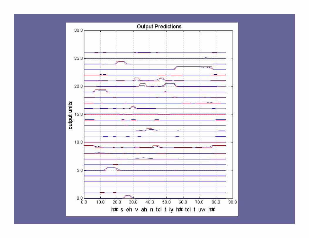
State trajectories suggest a use of history.

Discussion

• Anecdotal evidence suggests that LSTM learns a dynamic representation of phoneme segmentation

• Performance close to state-of-art HMMs

• More analysis and simulation required

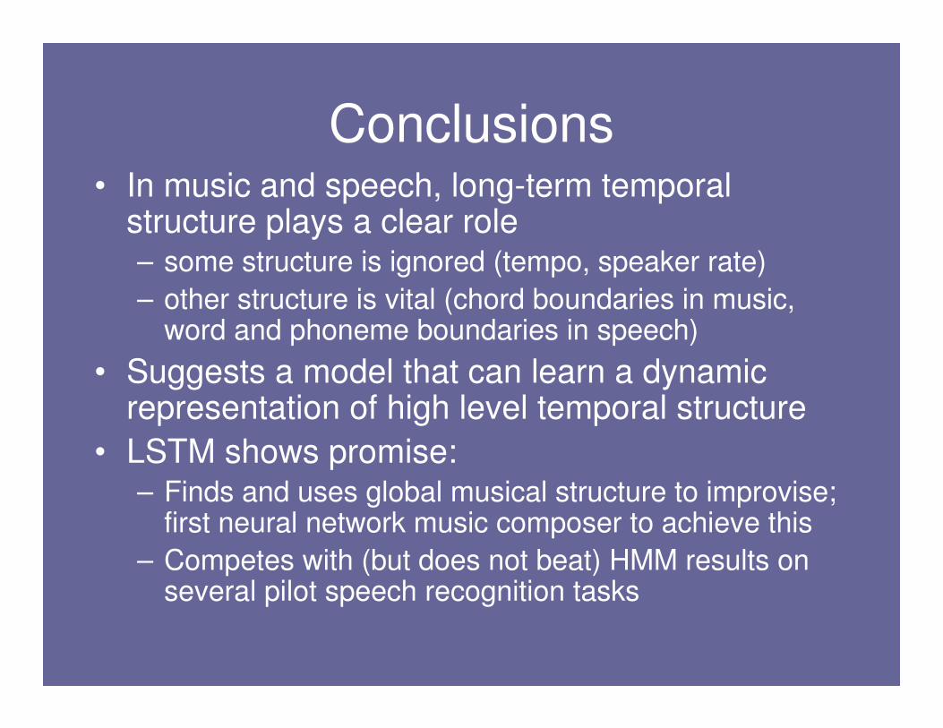
Conclusions• In music and speech, long-term temporal

structure plays a clear role– some structure is ignored (tempo, speaker rate)

– other structure is vital (chord boundaries in music, word and phoneme boundaries in speech)

• Suggests a model that can learn a dynamic representation of high level temporal structure

• LSTM shows promise:– Finds and uses global musical structure to improvise;

first neural network music composer to achieve this

– Competes with (but does not beat) HMM results on several pilot speech recognition tasks

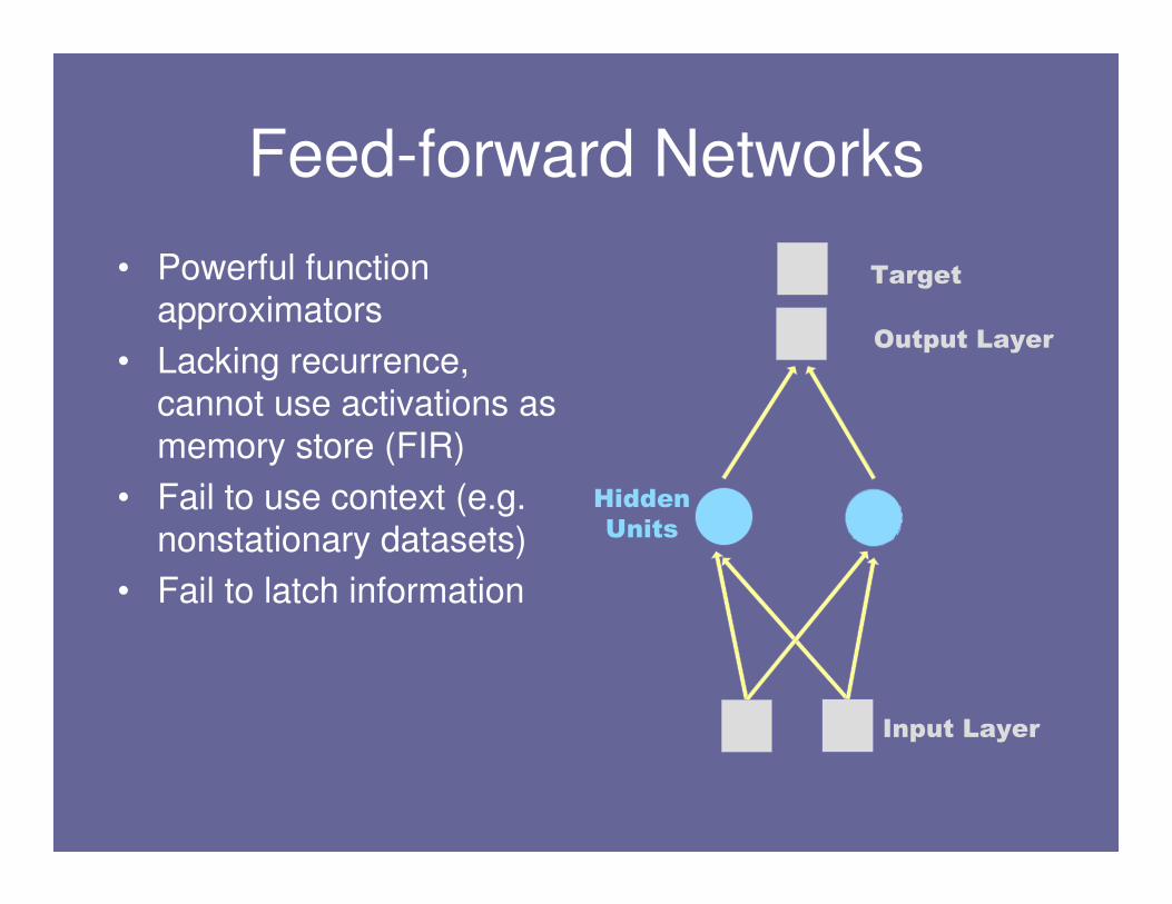
Feed-forward Networks

• Powerful function approximators

• Lacking recurrence, cannot use activations as

memory store (FIR)

• Fail to use context (e.g. nonstationary datasets)

• Fail to latch information

Hidden

Units

Input Layer

Output Layer

Target

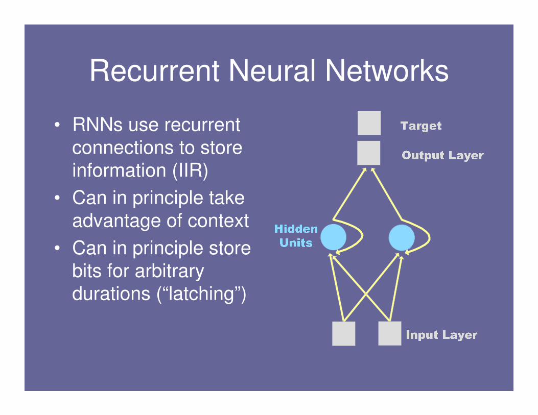
Recurrent Neural Networks

• RNNs use recurrent

connections to store

information (IIR)

• Can in principle take

advantage of context

• Can in principle store

bits for arbitrary

durations (“latching”)

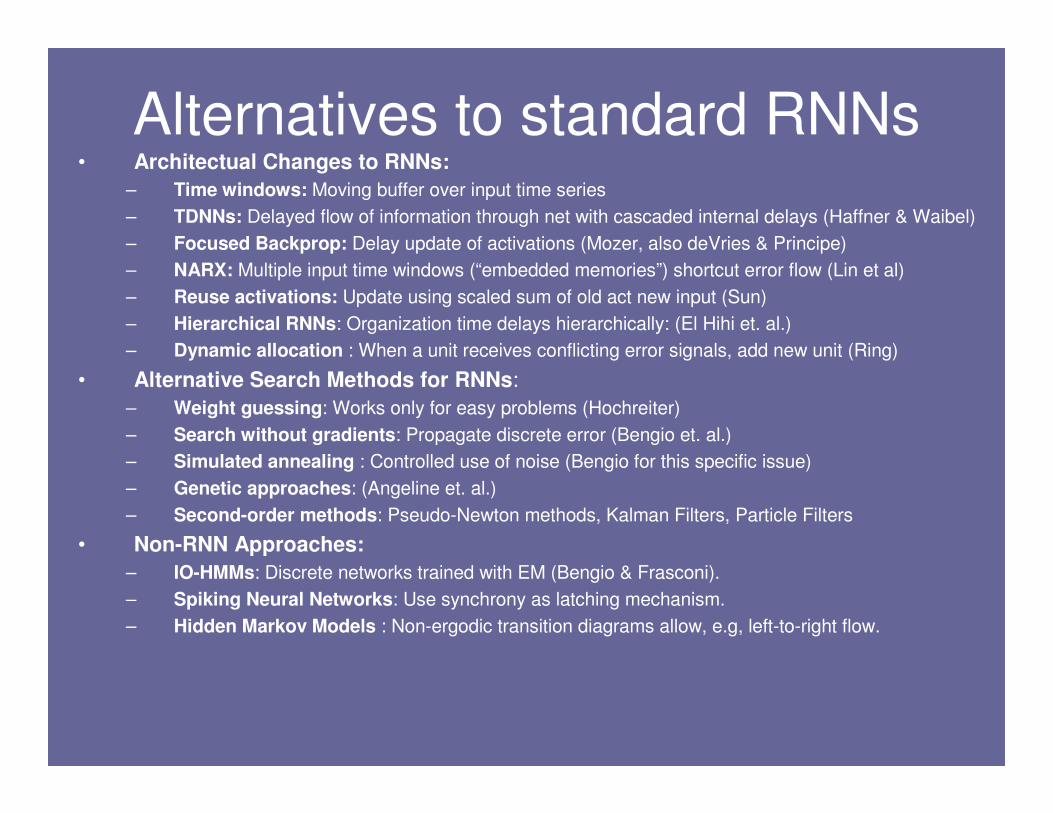
Alternatives to standard RNNs• Architectual Changes to RNNs:

– Time windows: Moving buffer over input time series

– TDNNs: Delayed flow of information through net with cascaded internal delays (Haffner & Waibel)

– Focused Backprop: Delay update of activations (Mozer, also deVries & Principe)

– NARX: Multiple input time windows (“embedded memories”) shortcut error flow (Lin et al)

– Reuse activations: Update using scaled sum of old act new input (Sun)

– Hierarchical RNNs: Organization time delays hierarchically: (El Hihi et. al.)

– Dynamic allocation : When a unit receives conflicting error signals, add new unit (Ring)

• Alternative Search Methods for RNNs:

– Weight guessing: Works only for easy problems (Hochreiter)

– Search without gradients: Propagate discrete error (Bengio et. al.)

– Simulated annealing : Controlled use of noise (Bengio for this specific issue)

– Genetic approaches: (Angeline et. al.)

– Second-order methods: Pseudo-Newton methods, Kalman Filters, Particle Filters

• Non-RNN Approaches:

– IO-HMMs: Discrete networks trained with EM (Bengio & Frasconi).

– Spiking Neural Networks: Use synchrony as latching mechanism.

– Hidden Markov Models : Non-ergodic transition diagrams allow, e.g, left-to-right flow.

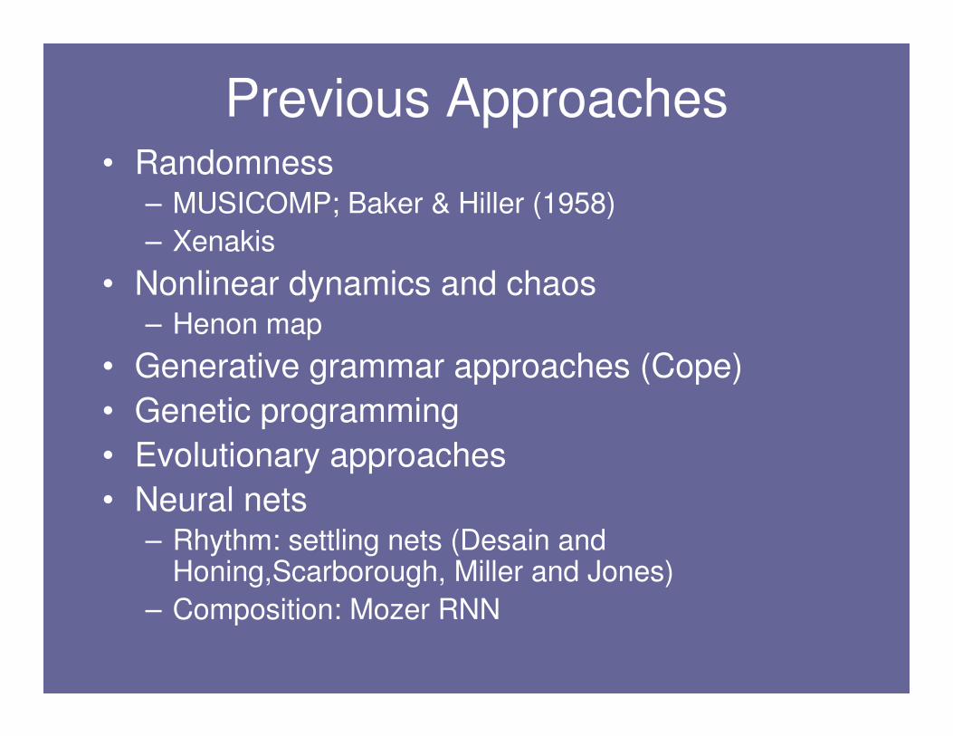
Previous Approaches• Randomness

– MUSICOMP; Baker & Hiller (1958)

– Xenakis

• Nonlinear dynamics and chaos– Henon map

• Generative grammar approaches (Cope)

• Genetic programming

• Evolutionary approaches

• Neural nets– Rhythm: settling nets (Desain and

Honing,Scarborough, Miller and Jones)

– Composition: Mozer RNN

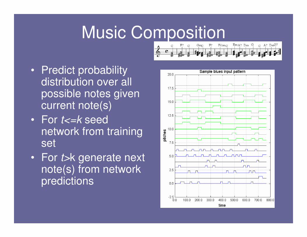
Music Composition

• Predict probability distribution over all possible notes given current note(s)

• For t<=k seed network from training set

• For t>k generate next note(s) from network predictions

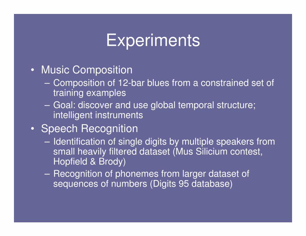
Experiments

• Music Composition– Composition of 12-bar blues from a constrained set of

training examples

– Goal: discover and use global temporal structure; intelligent instruments

• Speech Recognition– Identification of single digits by multiple speakers from

small heavily filtered dataset (Mus Silicium contest, Hopfield & Brody)

– Recognition of phonemes from larger dataset of sequences of numbers (Digits 95 database)

Output Gate Error (BP) ( )kk kc

S

v coutoutout vj

j

vjjjj

wszf δδ ∑∑ =′=

1)(

Compute errors and partials

LSTM Backward Pass

Cell State Error (BP) ( )kk kcouts vjjv

jc

wye δ∑=

mincfgt

jv

cm

jv

cm yyzgydSdSj

vjj

ˆ)(′+=Cell State Partials (RTRL)

minincfgt

jv

min

jv

min yzfzgydSdSjj

vjj

ˆ)()(,,′+=Input Gate Partials (RTRL)

Forget Gate Partials (RTRL)mfgtfgtcfgt

jv

mfgt

jv

mfgt yzfsydSdSjj

vjj

ˆ)(ˆ,,

′+=

Compute weight changes

• Weight changes into output gate proportional to output gate delta

• Weight changes into cell, input gate, forget gate proportional to partials

Advantages of RNNs

• Recurrent nets successfully used with some success for music composition (Mozer)

• Recurrent and non-recurrent nets successfully used for speech recognition in hybrid systems (Bengio; Boulard; Robinson)

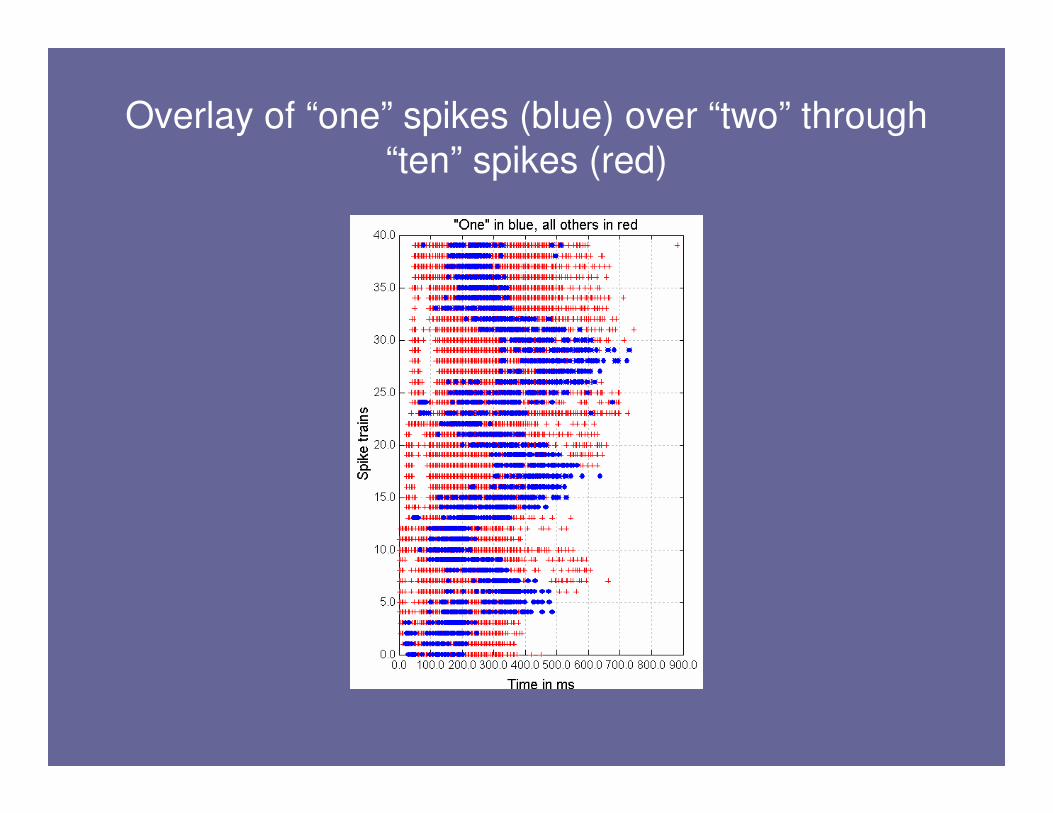
Overlay of “one” spikes (blue) over “two” through

“ten” spikes (red)

Future Work

• Intermediate tasks only: real task is speech recognition, not phoneme segmentation

• Not clear how to generate chains of phonemes from LSTM predictions

• Likely that LSTM would be one component in larger speech model (as in Boulard)

Advantages of LSTM

• Excels at finding temporally-distant information

in noise (Hochreiter & Schmidhuber 1997)

• Excels at formal grammar tasks requiring

counter-like memory: Reber grammar, CSLs like

anbncn (Gers & Schumidhuber 2001)

• Able to use gates to induce nonlinear oscillation

as timing and synchronization mechanism (Gers

et.al 2002, Eck & Schmidhuber 2002)