Hardness of Approximating Flow and Job Shop

Scheduling Problems∗

Monaldo MastrolilliIDSIA

Lugano, Switzerlandmonaldo@idsia.ch

Ola SvenssonRoyal Institute of Technology

Stockholm, Swedenosven@kth.se

April 15, 2011

Abstract

We consider several variants of the job shop problem which is a fun-damental and classical problem in scheduling. The currently best approx-imation algorithms have worse than logarithmic performance guarantee,but the only previously known inapproximability result says that it is NP-hard to approximate job shops within a factor less than 5/4. Closing thisbig approximability gap is a well-known and long-standing open problem.

This paper closes many gaps in our understanding of the hardness ofthis problem and answers several open questions in the literature. It isshown the first non-constant inapproximability result that almost matchesthe best known approximation algorithm for acyclic job shops. The samebounds hold for the general version of flow shops, where jobs are notrequired to be processed on each machine. Similar inapproximability re-sults are obtained when the objective is to minimize the sum of completiontimes. It is also shown that the problem with two machines and the pre-emptive variant with three machines have no PTAS.

1 Introduction

We consider the classical job shop scheduling problem together with the morerestricted flow shop problem. In the job shop problem we have a set of n jobs thatmust be processed on a given set M of m machines. Each job j consists of a chainof µj operations O1j , O2j , . . . , Oµjj . Operation Oij must be processed during pijtime units without interruption on machine mij ∈M . A feasible schedule is onein which each operation is scheduled only after all its preceding operations havebeen completed, and each machine processes at most one operation at a time.For any given schedule, let Cj be the completion time of the last operation ofjob j. We consider the natural and typically considered objectives of minimizingthe makespan Cmax = maxj Cj , and minimizing the sum of weighted completion

∗Different parts of this work have appeared in preliminary form in Proceedings of the49th Annual IEEE Symposium on Foundations of Computer Science (FOCS), 2008, pp. 583-592, and in Proceedings of the 36th International Colloquium on Automata, Languages andProgramming (ICALP), 2009, p. 677-688.

1

times∑wjCj . The goal is to find a feasible schedule which minimizes the

considered objective function. In the notation of Graham et al. [10] this problemis denoted as J ||γ, where γ denotes the objective function to be minimized.

In the flow shop scheduling problem (F ||γ) each job has exactly one operationper machine, and all jobs go through all the machines in the same order. Anatural generalization of the flow shop problem is to not require jobs to beprocessed on all machines, i.e., a job still requests the machines in compliancewith some fixed order but may not require to be processed on some of them.We will refer to this more general version as generalized flow shops or flow shopswith jumps (F |jumps|γ). Generalized flow shop scheduling (and thus flow shop)is a special case of acyclic job shop scheduling, which only requires that withineach job all operations are performed on different machines, which in turn is aspecial case of job shop scheduling. See Figure 1 for example instances of theaddressed problems.

m1

m2

m3

m1

m2

m3

m1

m2

m3

m1

m2

m3

(a) (b)

(c) (d)

Figure 1: Example of scheduling instances with three machines and two jobsdepicted in light and dark gray. a) Job shop instance – jobs may have severaloperations on each machine. b) Acyclic job shop instance – a job has at mostone operation per machine. c) Flow shop instance – each job has exactly oneoperation per machine and all the jobs are processed on the machines in thesame order. d) Generalized flow shop instance – jobs have at most one operationper machine and jobs are processed on the machines in the same order.

1.1 Literature Review

Job and flow shops have long been identified as having a number of importantpractical applications and have been widely studied since the late 50’s (thereader is referred to the survey papers of Lawler et al. [14] and of Chen, Potts& Woeginger [5]). To find a schedule that minimizes the makespan, or one thatminimizes the sum of completion times, was proved to be strongly NP-hard forflow shops (and thus job shops) in the 70’s, even for severely restricted instances(see e.g. [5]).

From then, many approximation methods have been proposed.1 Since the

1A ρ-approximation algorithm is a polynomial time algorithm that is guaranteed to return

2

quality of an approximation algorithm is measured by comparing the returnedsolution value with a polynomial time computable lower bound on the optimalvalue, the latter is very important. For a given instance, let C∗max denote theminimum makespan taken over all possible feasible schedules. If D denotes thelength of the longest job (the dilation), and C denotes the time units requestedby all jobs on the most loaded machine (the congestion), then lb = max[C,D] isa known trivial lower bound on C∗max. There is no known significantly strongerlower bound on C∗max, and all the proposed approximation algorithms for flowshops, acyclic job shops, job shops, and the more constrained case of permuta-tion flow shops have been analyzed with respect to this lower bound (see, e.g.,[7, 9, 15, 16, 17, 22]).

Even though the trivial lower bound might seem weak, a surprising result byLeighton, Maggs & Rao [15] says that for acyclic job shops, if all operations are ofunit length, then C∗max = Θ(lb). If we allow operations of any length, then Feige& Scheideler [7] showed that C∗max = O(lb · log lb log log lb) for acyclic job shops.They also showed their analysis to be nearly tight by providing acyclic job shopinstances with C∗max = Ω(lb · log lb/ log log lb). The proofs of the upper boundsin [7, 15] are nonconstructive and make repeated use of (a general version) of theLovasz local lemma. Algorithmic versions of the Lovasz local lemma [4] and thegeneral version [6], have later been used to obtain constructive upper boundsyielding a constant approximation algorithm for unit time acyclic job shops [16]and an O(log lb1+ε)-approximation algorithm for acyclic job shops [6], whereε > 0 is any constant.

Feige & Scheideler’s upper bound for acyclic job shops [7] is also the bestupper bound for the special case of flow shops. As flow shops have more struc-ture than acyclic job shops and no flow shop instances with C∗max = ω(lb)were known, one could hope for a significantly better upper bound for flowshops. The existence of such a bound was raised as an open question in [7].The strength of the lower bound lb is better understood for the related per-mutation flow shop problem, that is a flow shop problem with the additionalconstraint that each machine processes all the jobs in the same order. Potts,Shmoys & Williamson [18] gave a family of permutation flow shop instanceswith C∗max = Ω(lb ·

√min[m,n]). This lower bound was recently shown to be

tight, by Nagarajan & Sviridenko [17], who gave an approximation algorithmthat returns a permutation schedule with makespan O(lb ·

√min[m,n]).

The best approximation algorithms known for general J ||Cmax are an ap-proximation algorithm by Shmoys, Stein & Wein [22] with performance guar-antee O((log lb)2/ log log lb); later improved by a log log lb factor by Goldberg,Paterson, Srinivasan and Sweedyk [9].

When preemption is allowed, every operation can be temporarily interruptedand resumed later without any penalty. For any ε > 0, it is well-known thatwith only ε loss in the approximation factor, the preemptive job shop schedul-ing problem is equivalent to the nonpreemptive job shop scheduling problemwith unit processing times (see e.g. [3]). For acyclic job shop and flow shopscheduling with preemption, the best known result is due to Feige & Schei-deler [7] who showed that there always exists a preemptive schedule within aO(log log lb) factor of lb. For the general preemptive job shop problem, Bansalet al. [3] showed an O(logm/ log logm)-randomized approximation algorithm,

a solution that is within ρ times the optimal value.

3

and a (2 + ε)-approximation for a constant number of machines. In [3] theauthors also consider the preemptive two-machine job shop problem (denotedas J2|pmtn|Cmax) and present an approximation algorithm with ratio of about1.442 which improves the previous ratio of 1.5 [2, 21].

Whether the above algorithms for J ||Cmax and F ||Cmax are tight or evennearly tight, is a long standing open problem (see “Open problems 6 and 7”in [20]). The only known inapproximability result is due to Williamson et al. [23],and states that when the number of machines and jobs are part of the input,it is NP-hard to approximate F ||Cmax with unit time operations and at mostthree operations per job, within a ratio better than 5/4.

The situation is similar for the weighted sum of completions times objec-tive. Queyranne & Sviridenko [19] showed that an approximation algorithmfor the above mentioned problems that produces a schedule with makespan afactor O(ρ) away from the lower bound lb can be used to obtain an O(ρ)-approximation algorithms for other objectives, including the sum of weightedcompletion times. As a result, the above mentioned approximation guaranteesfor the makespan criteria also hold for the the sum of weighted completion timesobjective. The only known inapproximability result is by Hoogeveen, Schuur-man & Woeginger[11], who showed that F ||

∑Cj is NP-hard to approximate

within a ratio better than 1 + ε for some small ε > 0.Another open problem [20] is to understand whether there is a PTAS for

the general job shop problem with a constant number of machines. For thoseinstances where the number of machines and the number of operations per jobare constant, Jansen, Solis-Oba & Sviridenko [12] gave a PTAS for the makespancriteria. A similar result was later obtained by Fishkin, Jansen & Mastrolilli [8]for the weighted sum of completion times objective.

1.2 Results and Overview of Techniques

The main result of the paper gives an answer to ”Open Problem 7” by Schu-urman and Woeginger [20]) by showing that it is NP-hard to approximate thegeneralized flow shop problem (and therefore job shops) within any constantfactor. Under a stronger but widely believed assumption, the provided hard-ness result matches the best-known approximation algorithm for acyclic jobshops [7]. Similar inapproximability results are obtained when the objective isto minimize the sum of completion times.

Moreover, we solve negatively a question raised by Feige & Scheideler [7],by showing that the optimal solution for flow shops can be a logarithmic factoraway from lb. This implies that to obtain a better approximation guaranteefor flow shops it is necessary to improve the used lower bound on the optimalmakespan. When the number of machines and the number of operations per jobare assumed to be constant the job shop problem is known to admit a PTAS [12].This paper shows that both these restrictions are necessary to obtain a PTAS.Indeed we prove that the general job shop problem with 2 machines (denoted asJ2||Cmax) has no PTAS. The same limitation applies to the preemptive versionwith 3 machines (denoted as J3|pmtn|Cmax). The latter answers negatively anopen question raised by Bansal et al. [3]. A more detailed presentation of theresults is given in the following.

4

1.2.1 Generalized Flow Shops

Feige & Scheideler [7] showed their analysis to be essentially tight for acyclic jobshops. As flow shops are more structured than acyclic job shops, they raisedas an open question whether the upper bound for flow shop scheduling can beimproved significantly. Our first result resolves this question negatively.

Theorem 1 There exist flow shop instances with optimal makespan Ω(lb· log lblog log lb ).

Proof Overview. The construction of job shop instances with “large” makespanis presented in Section 2.1 and serves as a good starting point for reading Sec-tion 2.2 where the more complex construction of flow shop instances with “large”makespan is presented.

The job shop construction closely follows the construction in [7] with themain difference being that we do not require all operations of a job to be ofthe same length, which leads to a slightly better analysis. The main idea isto introduce jobs of different “frequencies”, with the property that two jobs ofdifferent frequencies essentially cannot be processed at the same time in anyfeasible schedule. Hence, a job shop instance with d jobs of different frequen-cies, all of them of length D, has optimal makespan Ω(d · D). Moreover, theconstruction satisfies lb = C = D = 3d and it follows that the job shop instancehas optimal makespan Ω(d · 3d), which can be written as Ω(lb · log lb).

The construction of flow shop instances with “large” makespan is more com-plicated, as each job is required to have exactly one operation for every machine,and all jobs are required to go through all the machines in the same order. Themain idea is to start with the aforementioned job shop construction, which has“very cyclic” jobs, i.e., jobs have many operations on a single machine. The flowshop instance is then obtained by “copying” the job shop instance several timesand instead of having cyclic jobs we let the i-th “long-operation” of a job to beprocessed by a machine in the i-th copy of the original job shop instance. Fi-nally, we insert additional zero-length operations to obtain a flow shop instance.By carefully choosing the different frequencies we can show that the constructedflow shop instance will have essentially the same optimal makespan as the jobshop instance we started with. The slightly worse bound, Ω(lb · log lb/ log log lb)instead of Ω(lb · log lb), arises from additional constraints on the design of fre-quencies.

If we do not require a job to be processed on all machines, i.e. generalizedflow shops, we prove that it is hard to improve the approximation guarantee.Theorem 2 shows that generalized flow shops, with the objective to either min-imize makespan or sum of completion times 2, have no constant approximationalgorithm unless P = NP .

Theorem 2 For all sufficiently large constants K, it is NP-hard to distinguishbetween generalized flow shop instances that have a schedule with makespan 2K ·lb and those that have no solution that schedules more than half of the jobswithin (1/8)K

125 (logK) · lb time units. Moreover this hardness result holds for

generalized flow shop instances with bounded number of operations per job, thatonly depends on K.

2Note that Theorem 2 implies that for sufficiently large constants K, it is NP-hard to

distinguish whether∑Cj ≤ n · 2K · lb or

∑Cj ≥ n

2· (1/8) ·K

125

(logK) · lb, where n is thenumber of jobs.

5

Proof Overview. The reduction is from the NP-hard problem of decidingwhether a graph G with degree bounded by a constant ∆ can be colored using“few” colors or has no “large” independent set (see Theorem 7). In Section 3.1we present a relatively easy reduction to the job shop problem which serves asa good starting point for reading the more complex reduction for the general-ized flow shop problem presented in Section 3.2. The main idea is as follows.Given a graph G with bounded degree ∆, we construct a generalized flow shopinstance S, where all jobs have the same length D and all machines the sameload C = D. Hence, lb = C = D. Instance S has a set of jobs for each vertexin G. By using jobs of different frequencies, as done in the gap construction, wehave the property that “many” of the jobs corresponding to adjacent verticescannot be scheduled in parallel in any feasible schedule. On the other hand,by letting jobs skip the machines corresponding to non-adjacent vertices, jobscorresponding to an independent set in G can be scheduled in parallel (theiroperations can overlap in time) in a feasible schedule. For the reduction to bepolynomial it is crucial that the number of frequencies is relatively small. How-ever, to ensure the desired properties, jobs corresponding to adjacent verticesmust be of different frequencies. We resolve this by using the fact that G hasbounded degree. Since the graph G has degree of at most ∆ we can in polyno-mial time partition its vertices into ∆ + 1 independent sets. As two jobs onlyneed to be assigned different frequencies if they correspond to adjacent vertices,we only need a constant (∆ + 1) number of frequencies.

The analysis follows naturally: a set of jobs corresponding to an independentset can be scheduled in parallel. Hence, if the graph G can be colored with few,say F , colors then there is a schedule of S with makespan O(F · lb). Finally,if there is a schedule where at least half the jobs finish within L · lb time unitsthen jobs corresponding to at least a fraction Ω(1/L) of the vertices overlap atsome point in the schedule. As the jobs overlap, they correspond to a fractionΩ(1/L) of vertices that form an independent set. It follows that if the graph hasno large independent set, then the generalized flow shop instance has no shortschedule.

By making a stronger assumption, we give a hardness result that essentiallyshows that the current approximation algorithms for generalized flow shops (andacyclic job shops), with both makespan and sum of weighted completion timesobjectives, are tight.

Theorem 3 Let ε > 0 be an arbitrarily small constant. There is noO((log lb)1−ε)-approximation algorithm for F |jumps|Cmax or F |jumps|

∑Cj,

unless NP ⊆ ZTIME(2lognO(1/ε)

).

Proof Overview. The construction of the generalized flow shop instance isthe same as in the proof of Theorem 2. To obtain the stronger result we usea stronger hardness result for graph coloring (see Theorem 8). The tricky partis that the graph no longer has a small bounded degree. We overcome thisdifficulty by a randomized process that preserves the desired properties of thegraph with an overwhelming probability (see Lemma 14).

For flow shops, the consequences of Theorem 1 and Theorem 3 are among othersthat in order to improve the approximation guarantee, it is necessary to (i)

6

improve the used lower bound on the optimal makespan and (ii) use the factthat a job needs to be processed on all machines.

From Theorem 2 and Theorem 3 we have the following for the more generaljob shop problem.

Theorem 4 Job Shops are NP-hard to approximate within any constant andhave no O

((log lb)1−ε)-approximation algorithm for any ε > 0, unless NP ⊆

ZTIME(2lognO(1/ε)

).

1.2.2 Job Shop with Bounded Number of Machines:

In [12], a PTAS was given for the (preemptive) job shop problem, where boththe number of machines and the number of operations per job are assumed tobe constant. Our second result shows that both these restrictions are necessaryto obtain a PTAS (that one needs to restrict the number of machines followsfrom the work in [23]).

Theorem 5 The job shop problem with 2 machines (J2||Cmax) has no PTASunless NP ⊆ DTIME(nO(logn)).

Proof Overview. In Section 4.1, we prove the result by presenting a gap-preserving reduction from the independent set problem in cubic graphs, i.e.,graphs where all vertices have degree three (see Theorem 9).

Given a cubic graph G we construct an instance S of J2||Cmax as follows.The instance has a “big” job, called jb, whose length will equal the makespanin the completeness case. Its operations are divided into four parts, called theedge-, tail-, slack-, and remaining-part. There is also a vertex job for eachvertex. We again use the technique of introducing different frequencies of jobs;this time to ensure that, without delaying job jb, two jobs corresponding toadjacent vertices cannot both complete before the end of the tail-part of job jb.

The analysis now follows from selecting the lengths of the different parts of jbsuch that in the completeness case we can schedule all jobs, corresponding to a“big” independent set of G, in parallel with the edge- and tail-part of job jb andthe remaining jobs are scheduled in parallel with the slack- and remaining-partof job jb. In contrast, in the soundness case, as G has no “big” independentset, we can, without delaying the schedule, only schedule relatively few jobs inparallel with the edge- and tail-part of job jb. The remaining jobs, relativelymany, will then require more time units than the total length of the slack- andremaining-part of job jb and it follows that the schedule will have makespanlarger than the length of jb.

The reduction runs in time nO(f), where f is the number of frequencies. Withour current techniques we need O(log n) frequencies and hence the assumptionused in the statement of Theorem 5.

For the general preemptive job shop problem, Bansal et al. [3] showed a(2 + ε)-approximation for a constant number of machines. According to [3], itis an an “outstanding open question” to understand whether there is a PTASfor the general preemptive job shop with a constant number of machines. Wesolve (negatively) the open question raised in [3].

7

Theorem 6 The preemptive job shop problem with 3 machines (J3|pmtn|Cmax)has no PTAS unless NP ⊆ DTIME(nO(logn)).

The proof of Theorem 6 it is more involved than the proof of Theorem 5 but ithas a similar structure. We remark that the approximability of J2|pmtn|Cmaxis still open.

1.3 Preliminaries

When considering a schedule we shall say that two jobs (or operations) overlapor are scheduled in parallel for t time units if t time units of them are processedat the same time on different machines. For a given graph G, we let χ(G) andα(G) denote the chromatic number of G and the size of a maximum independentset of G, respectively. We shall also denote the maximum degree of graph G by∆(G), where we sometimes drop G when it is clear from the context.

Our reductions to the job shop problem with unbounded number of machinesuse results by Khot [13], who proved that even though we know that the graphis colorable using K colors it is NP-hard to find a coloring that uses less thanK

125 (logK) colors, for sufficiently large constants K. The result was obtained by

presenting a polynomial time reduction that takes as input a SAT formula φtogether with a sufficiently large constant K and outputs an n-vertex graph G

with degree at most 2KO(logK)

such that (completeness) if φ is satisfiable thenG can be colored using at most K colors and (soundness) if φ is not satisfiable

then G has no independent set containing n/K125 (logK) vertices (see Section 6

in [13]). Note that the soundness case implies that any feasible coloring of the

graph uses at least K125 (logK) colors. We let G[c, f ] be the family of graphs

that either can be colored using c colors or have no independent set containinga fraction f of the vertices. The following theorem (not stated in this formin [13]) summarizes the result obtained.

Theorem 7 ([13]) For all sufficiently large constants K, it is NP-hard to de-

cide if a graph in G[K, 1/K125 (logK)] can be colored using K colors or has no

independent set containing a fraction 1/K125 (logK) of the vertices. Moreover this

hardness result holds for graphs with degree at most 2KO(logK)

.

By using a stronger assumption, we can let K be a function of the number ofvertices. Again, the stronger statement (not explicitly stated in [13]) followsfrom the soundness analysis.

Theorem 8 ([13]) There exists an absolute constant γ > 0 such that for allK ≤ 2(logn)γ , there is no polynomial time algorithm that decides if an n-vertex graph in G[K, 1/KΩ(logK)] can be colored using K colors or has no in-dependent set containing a fraction 1/KΩ(logK) of the vertices, unless NP ⊆DTIME(2O(logn)O(1)

).

Our reduction to J2||Cmax uses the following result by Alimonti and Kann [1].A cubic graph is a graph where all vertices have degree three.

Theorem 9 ([1]) There exist positive constants β, α with β > α, so that it isNP -hard to distinguish between n-vertex cubic graphs that have an independentset of size β · n and those that have no independent set of size α · n.

8

2 Job and Flow Shop Instances with Large Makespan

We first exhibit a family of instances of general job shop scheduling for which it isrelatively simple to show that any optimal schedule is of length Ω(lb·log lb). Thiscomplements3 and builds on the bound by Feige & Scheideler [7], who showed theexistence of job shop instances with optimal makespan Ω(lb · log lb/ log log lb).We then use this construction as a building block in the more complicated flowshop construction.

2.1 Job Shops with Large Makespan

2.1.1 Construction

For any integer d ≥ 1 consider the job shop instance with d machines m1, . . . ,md

and d jobs j1, . . . , jd. We say that job ji has frequency i, which means that it has3i so-called long-operations on machine mi, each one of them requires 3d−i timeunits. Between any two consecutive long-operations, job ji has short-operationsthat require 0 time units on the machines m1, . . . ,mi−1. Note that the lengthof all jobs and the load on all machines are 3d, which we denote by lb. SeeFigure 2 for an example of the construction.

m1

m2

m3

Figure 2: An example of the construction with d = 3. The long-operationsof jobs of frequency 1, 2 and 3 are depicted in light, medium, and dark gray,respectively. Job ji has 3i long-operations on machine mi, for i ∈ 1, 2, 3.

2.1.2 Analysis

Fix an arbitrary feasible schedule of the jobs. We shall show that the length ofthe schedule must be Ω(lb · log lb).

Lemma 10 For i, j : 1 ≤ i < j ≤ d, the number of time units during whichboth ji and jj perform operations is at most lb

3j−i .

Proof. During the execution of a long-operation of ji (that requires 3d−i timeunits), job jj can complete at most one long-operation that requires 3d−j timeunits (since its short-operation on machine mi has to wait). As ji has 3i long-operations, the two jobs can perform operations at the same time during at

most 3i · 3d−j = 3d

3j−i = lb3j−i time units.

It follows that, for each i = 1, . . . , d, at most a fraction 1/3 + 1/32 + · · · +1/3i ≤ 1/3+1/32 + · · ·+1/3d ≤ 1

3−1 = 1/2 of the time spent for long-operationsof a job ji is performed at the same time as long-operations of jobs with lowerfrequency. Hence a feasible schedule has makespan at least d · lb/2. As d =Ω(log lb) (recall that lb = 3d), the optimal makespan of the constructed jobshop instance is Ω(lb · log lb).

3In their construction all operations of a job have the same length which is not the casefor our construction.

9

2.2 Flow Shops with Large Makespan

2.2.1 Construction

For sufficiently large integers d and r, consider the flow shop instance defined asfollows (we refer to Figure 3 for an example of the construction with d = r = 2):

• There are r2d groups of machines4, denoted by M1,M2, . . . ,Mr2d . Eachgroup Mg consists of d machines mg,1,mg,2, . . . ,mg,d (one for each fre-quency). Finally the machines are ordered in such a way that mg,i isbefore mh,j if either (i) g < h or (ii) g = h and i > j. The latter case willensure that, within each group of machines, long-operations of jobs withhigh frequency will be scheduled before long-operations of jobs with lowfrequency, a fact that will be used in the proof of Lemma 12.

(In the example of Figure 3 there are 24 groups of machines, where ma-chines mg,1,mg,2 are those that belong to group Mg. The only long-operations that can be scheduled on machine mg,i are those belonging tojobs of frequency i. In top down order, note that machine mg,2 is beforemg,1 and before mh,i for any g < h and i ∈ 1, 2.)

• For each frequency f = 1, . . . , d, there are r2(d−f) groups of jobs, denotedby Jf1 , J

f2 , . . . , J

fr2(d−f) . Each group Jfg consists of r2f copies, referred to

as jfg,1, jfg,2, . . . , j

fg,r2f , of the job that must be processed during r2(d−f)

time units on the machines

ma+1,f ,ma+2,f , . . . ,ma+r2f ,f where a = (g − 1) · r2f

and during 0 time units on all the other machines that are required tocreate a flow shop instance. Let Jf be the set of jobs that correspond tofrequency f , i.e., Jf = jfg,a : 1 ≤ g ≤ r2(d−f), 1 ≤ a ≤ r2f.(In the example of Figure 3 there are four groups of jobs with frequencyone, and one group with frequency two. Every group of frequency onehas four identical jobs: in the figure, on machine m1,1 the leftmost oper-ations of equal length are the first operations of the jobs in group J1

1 =j1

1,1, . . . , j11,4; the 4 leftmost gray operations in cascade are the operations

of job j11,2; the leftmost operations on machines m13,1,m14,1,m15,1,m16,1

belong to the last group J14 of frequency one. The rightmost (smaller)

operations are those belonging to the unique group J21 of frequency two;

the rightmost gray operations in cascade are, respectively, the first andthe last 4 operations out of the 16 operations of job j2

1,2.)

Note that the length of any job and the load on any machine are r2d, whichequals lb. Moreover, the total number of machines and the total number of jobsare both r2d · d. In the subsequent we will call the operations that require morethan 0 time units long-operations and the operations that only require 0 timeunits short-operations.

4These groups of machines “correspond” to copies of the job shop instance in subsection 2.1.

10

m1,2m1,1m2,2m2,1

m16,2m16,1

Figure 3: An example of the construction for flow shop scheduling with r =d = 2. Only long-operations on the first 4 and last 4 groups of machines aredepicted. The long-operations of one job of each frequency are highlighted indark gray.

2.2.2 Analysis

We shall show that the length of any feasible schedule must be Ω(lb ·min[r, d]).As lb = r2d, instances constructed with r = d have optimal makespan Ω(lb ·log lb/ log log lb).

Fix an arbitrarily feasible schedule for the jobs. We start by showing auseful property. For a job j, let dj(i) denote the delay between its i-th and(i + 1)-th long-operations, i.e., the time units between the end of job j’s i-thlong-operation and the start of its (i+1)-th long-operation (let dj(i) =∞ for thelast long-operation). We say that the i-th long-operation of a job j of frequency

f is good if dj(i) ≤ r2

4 · r2(d−f).

Lemma 11 If the schedule has makespan less than r · lb then the fraction ofgood long-operations of each job is at least

(1− 4

r

).

Proof. Assume that the considered schedule has makespan less than r · lb.Suppose toward contradiction that there exists a job j of frequency f so that jhas at least 4

r r2f long-operations that are not good. But then the length of j is

at least 4r r

2f · r2

4 · r2(d−f) = r · r2d = r · lb, which contradicts that the makespan

of the considered schedule is less than r · lb.We continue by analyzing the schedule with the assumption that its makespan

is less than r · lb (otherwise we are done). In each group Mg of machines wewill associate a set Tg,f of time intervals for each frequency f = 1, . . . , d. Theset Tg,f contains the time intervals corresponding to the first half of all goodlong-operations scheduled on the machine mg,f . For intuition of the followinglemma see Figure 4.

Lemma 12 Let k, ` : 1 ≤ k < ` ≤ d be two different frequencies. Then the setsTg,k and Tg,` , for all g : 1 ≤ g ≤ r2d, contain disjoint time intervals.

Proof. Suppose toward contradiction that there exist time intervals tk ∈ Tg,kand t` ∈ Tg,` that overlap, i.e., tk ∩ t` 6= ∅. Note that tk and t` correspondto good long-operations of jobs of frequencies k and `, respectively. Let ussay that the good long-operation corresponding to t` is the a-th operation of

11

some job j. Note that, since j has a long-operation on machine mg,`, jobj has frequency `. As t` and tk overlap, the a-th long-operation of j mustoverlap the first half of the long-operation corresponding to tk. As job j has ashort operation on machine mg,k after its long-operation on machine mg,` (recallthat machines are ordered mg,d,mg,d−1, . . . ,mg,1 and ` > k), job j’s (a+ 1)-thoperation must be delayed by at least r2(d−k)/2 − r2(d−`) time units and thus

dj(a) > r2(d−k)/2 − r2(d−`) > r2

4 r2(d−`) (using ` > k), which contradicts that

the a-th long-operation of job j is good.

a+1

a

delay contradicts thata-th operation is good

mg,!

mg,k

mg+1,!

Figure 4: The intuition behind the proof of Lemma 12.

Let L(Tg,f ) denote the total time units covered by the time intervals in Tg,f .

We continue by showing that there exists a g such that∑df=1 L(Tg,f ) ≥ lb

4 · d.With this in place, it is easy to see that any schedule has makespan Ω(d · lb)since all the time intervals Tg,f : f = 1, . . . , d are disjoint (Lemma 12).

Lemma 13 There exists a g ∈ 1, . . . , r2d such that

d∑f=1

L(Tg,f ) ≥ lb

4· d

Proof. As∑df=1 L(Tg,f ) adds up the time units required by the first half of

each good long-operation scheduled on a machine in Mg, the claim follows byshowing that there exists a group of machines Mg from M1,M2, . . . ,Mr2d sothat the total time units required by the good long-operations on the machinesin Mg is at least lb·d

2 .By lemma 11 we have that the good long-operations of each job require at

least lb ·(1− 4

r

)time units. Since the total number of jobs is r2dd the total time

units required by all good long-operations is at least lb ·(1− 4

r

)· r2dd. As there

are r2d many groups of machines, a simple averaging argument guarantees thatin at least one group of machines, say Mg, the total time units required by thegood long-operations on the machines in Mg is at least lb ·

(1− 4

r

)d > lb · d/2

for a sufficiently large r.

12

3 Hardness of Job Shops and Generalized FlowShops

Theorem 2 and Theorem 3 are proved by presenting a gap-preserving reduction,Γ, from the graph coloring problem to the generalized flow shop problem, thathas two parameters, r and d. Given an n-vertex graph G whose vertices arepartitioned into d independent sets, it computes in time polynomial in n and rd,a generalized flow shop instance S(r, d) where vertices are mapped to jobs. Byusing jobs of different frequencies, as done in the gap construction, we have theproperty that “many” of the jobs corresponding to adjacent vertices cannot bescheduled in parallel in any feasible schedule. On the other hand, by letting jobsskip those machines corresponding to non-adjacent vertices, jobs correspondingto an independent set in G can be scheduled in parallel (their operations canoverlap in time) in a feasible schedule. This ensures that the following com-pleteness and soundness hold for the resulting generalized flow shop instanceS(r, d).

• (Completeness) If G can be colored using L colors then C∗max ≤ lb · 2L.

• (Soundness) For any L ≤ r. Given a schedule where at least half the jobsfinish within lb ·L time units, we can find an independent set of G of sizen/(8L), in time polynomial in n and rd.

In the proposed construction all jobs have the same length r2d and all ma-chines the same load r2d. Hence, lb = r2d. Instance S(r, d) has a set of r2d jobsand a set of r2d machines for each vertex in G. The total number of jobs andthe total number of machines are thus both r2dn. Moreover, each job has atmost dr2d operations.

In Section 3.1, we present a reduction with somewhat stronger properties forthe job shop problem. As the reduction is relatively simple, it serves as a goodstarting point before reading the similar but more complex reduction Γ for thegeneralized flow shop problem. Before continuing, let us see how the reductionΓ, with the aforementioned properties, is sufficient for proving Theorem 2 andTheorem 3.

3.0.3 Proof of Theorem 2

By Theorem 7, for sufficiently large K and ∆ = 2KO(logK)

, it is NP-hard todecide if an n-vertex graph G in G[K, 1/K

125 (logK)] with bounded degree ∆ has

χ(G) ≤ K or α(G) ≤ n

K125 (logK)

.

As the vertices of a graph with bounded degree ∆ can, in polynomial time,be partitioned into ∆ + 1 independent sets, we can use Γ with parametersd = ∆ + 1 and r = K

125 (logK) (r is chosen such that the condition L ≤ r in

the soundness case of Γ is satisfied for L = K125 (logK)/8). It follows by the

completeness case and soundness case of Γ that it is NP-hard to distinguish ifthe obtained scheduling instance has a schedule with makespan at most lb · 2Kor no solution schedules more than half of the jobs within lb ·K 1

25 (logK)/8 timeunits. Moreover, each job has at most dr2d operations, which is a constant thatonly depends on K.

13

3.0.4 Proof of Theorem 3

The proof is similar to the proof of Theorem 2 with the exception that thegraphs have no longer bounded degree. Note that, since the construction isexponential in d, we aim for a “small” value of d that ensures that two jobscorresponding to two adjacent nodes get different frequencies. This can be doneif the graph can be colored with “few” colors. If the graph has “small” boundeddegree ∆, then d = ∆ + 1 suffices to ensure the above property. Otherwise, thefollowing lemma says that we can construct another graph G′ with “similar”properties as G, but G′ is easily colorable with at most (log n)δ colors, which issufficiently “small” for our purposes.

When using probabilistic arguments for graphs with n vertices, we shall usethe term overwhelming (negligible, respectively) to denote probability that tendsto 1 (to 0, respectively) as n tends to infinity.

Lemma 14 For any constant δ ≥ 1, given an n-vertex graph G = (V,E), wecan construct in randomized polynomial time a subgraph G′ = (V,E′) of G withE′ ⊆ E such that

1. The vertices are partitioned into (log n)δ sets, each set forms an indepen-dent set in G′.

2. χ(G′) ≤ χ(G).

3. With overwhelming probability the following holds: given an independentset of G′, with n

(logn)δ−1 vertices, we can find an independent set of G withn

(logn)δvertices, in polynomial time.

Proof. Given an n-vertex graph G = (V,E), we give a probabilistic construc-tion of G′ = (V,E′). Each vertex v ∈ V is assigned independently, uniformly atrandom to one of the sets I1, I2, . . . , I(logn)δ . Let E′ ⊆ E be those edges thatare incident to vertices placed in different sets, i.e., an edge is deleted from Eto yield E′ if and only if it is adjacent to two vertices u ∈ Ii and v ∈ Ii for somei : 1 ≤ i ≤ (log n)δ.

The graph G′ obviously satisfies the first two properties in the lemma. Wecontinue by showing that G′ satisfies property 3. In fact, we show that the fol-lowing stronger property holds with overwhelming probability: any independentset I ′ of G′, with |I ′| = n

(logn)δ−1 , induces a subgraph of G with at least n(logn)δ

maximal connected components. This is done by proving that if a subset V ′ ofn/(log n)δ−1 vertices induces a subgraph of G with less than n

(logn)δmaximal

connected components, then the probability that V ′ is an independent set of G′

is negligible.Fix a set V ′ ⊆ V of n/(log n)δ−1 vertices and let H be the subgraph of G

induced by V ′. Assuming that H can be partitioned into s maximal connectedcomponents, with s < n

(logn)δ, we calculate the probability that V ′ forms an in-

dependent set in G′. Let H1, H2, . . . ,Hs denote the maximal connected compo-nents of H. We use |H`|, for ` : 1 ≤ ` ≤ s, to denote the number of vertices of H`.If the vertices of H form an independent set in G′ then all vertices of a connectedcomponent must be placed in the same set Ii, for some i : 1 ≤ i ≤ (log n)δ. Theprobability that this happens, for a connected component with k vertices, is at

most(

1logn

)δ(k−1)

. As the different maximal connected components are inde-

14

pendent, the probability that V ′ forms an independent set in G′ is at most(1

log n

)δ(|H1|−1)(1

log n

)δ(|H2|−1)

. . .

(1

log n

)δ(|Hs|−1)

=

(1

log n

)δ(∑si=1 |Hi|−s)

.

As∑si=1 |Hi| = |V ′| = n/(log n)δ−1 and s < n

(logn)δ, the probability that V ′

forms an independent set in G′ is at most(1

log n

)δ·n/(logn)δ−1·(1−1/ logn)

.

The number of ways to fix the set V ′ is at most(n

n/(log n)δ−1

)≤ (e · log n)

(δ−1)n/(logn)δ−1

.

Hence, the union bound implies that the probability that graph G′ fails to satisfyproperty 3 is at most(

1

log n

)δ·n/(logn)δ−1·(1−1/ logn)

· (e · log n)(δ−1)n/(logn)δ−1

which tends to 0 as n tends to infinity.

Assuming NP 6⊆ DTIME(2O(logn)O(1)

), Theorem 8 with K = log n saysthat there is no polynomial algorithm that decides if an n-vertex graph G inG[log n, 1/(log n)Ω(log logn)] has

χ(G) ≤ log n or α(G) ≤ n

(log n)Ω(log logn).

Given an n-vertex graph G in G[log n, 1/(log n)Ω(log logn)], we construct graphG′ from G by applying Lemma 14 with δ = 3/ε, where ε > 0 is an arbitrarilysmall constant. We then obtain a generalized flow shop instance S from G′

by using Γ with parameters r = (log n)δ−1 and d = (log n)δ. The size of S is

O(r2dn ·∆r2d) = O(2O(logn)O(1/ε)

) and lb = r2d = (log n)2(δ−1)(logn)δ and hencelog lb ≤ (log n)δ+1 (for large enough n).

The analysis is straightforward:

• (Completeness) If χ(G) ≤ log n then χ(G′) ≤ log n and, by the complete-ness case of Γ, there is a schedule of S with makespan lb · 2 log n.

• (Soundness) Assuming that the probabilistic construction of G′ succeeded,we have α(G) ≤ n

nΩ(log logn)⇒ α(G′) ≤ n

(logn)δ−1 , which in turn implies by

the soundness case of Γ that no solution schedules more than half the jobswithin lb · (log n)δ−1/8 time units (recall that r was chosen to be greaterthan (log n)δ−1/8).

The probabilistic construction of G′ succeeds with overwhelming probabil-ity. Furthermore, given a schedule, we can detect such a failure in polynomialtime and repeat the reduction. It follows that an approximation algorithm

for F |jumps|Cmax with performance guarantee (logn)δ−1/82 logn = (log n)δ−2/16 or

15

an approximation algorithm for F |jumps|∑Cj with performance guarantee

(n/2)·(logn)δ−1/82n·logn = (log n)δ−2/32 would imply thatNP ⊆ ZTIME(2O(logn)O(1/ε)

).Finally we note that δ was chosen so that for large enough n we have

(log lb)1−ε ≤ (log n)(1−ε)(δ+1) = (log n)3/ε+1−3−ε =

(log n)δ−2−ε < 1/32 · (log n)δ−2.

3.1 Job Shops

In this section we give and analyze a somewhat stronger reduction than Γ forthe general job shop problem. The number of operations per job is at most(∆ + 1)rd, the number of jobs and the number of machines are n, and thesoundness case says that, given a schedule with makespan lb ·L, we can, in timepolynomial in n and rd, find an independent set of G of size (1 − ∆

r )n/L.5 Asthe reduction is relatively simple, it serves as a good starting point for readingthe more complex reduction to the generalized flow shop problem.

3.1.1 Construction

Given an n-vertex graph G = (V,E) whose vertices are partitioned into d in-dependent sets, we create a job shop instance S(r, d), where r and d are theparameters of the reduction. Instance S(r, d) has a machine mv and a job jvfor each vertex v ∈ V . We continue by describing the operations of the jobs.Let I1, I2, . . . Id denote the independent sets that form a partition of V . A jobjv that corresponds to a vertex v ∈ Ii, for some i : 1 ≤ i ≤ d, has a chain of ri

long-operations O1,jv , O2,jv , . . . , Ori,jv , each of them requiring rd−i time units,that must be processed on the machine mv. Between two consecutive long-operations Op,jv , Op+1,jv , for p : 1 ≤ p < ri, we have a set of short-operationsplaced on the machines mu : u, v ∈ E (the machines corresponding to adja-cent vertices) in some order. A short-operation requires time 0. For an exampleof the construction see Figure 5.

Remark 15 The construction has n machines and n jobs. Each job has lengthrd and each machine has load rd. Hence, lb = rd. Moreover, the number ofoperations per job is at most (∆ + 1)rd.

A

B C mA

mB

mC

Figure 5: An example of the reduction with r = 4, d = 2, I1 = A, and I2 =B,C. Note that jobs only have short-operations on machines correspondingto adjacent vertices. (The jobs corresponding to A,B, and C are depicted tothe left, center, and right respectively.)

5The condition that r needs to be greater than ∆ can be removed as done in the analysisof generalized flow shops. In this section we have chosen to provide a simpler analysis, whichstill describes most of the ideas used in the flow shop analysis.

16

3.1.2 Completeness

We prove that if the graph G can be colored with L colors then there is a“relatively short” solution to the job shop instance (see Figure 6).

Lemma 16 If χ(G) = L then there is a schedule of S(r, d) with makespan lb·L.

Proof. Let V1, V2, . . . , VL be a partition of V into L independent sets. Con-sider one of these sets, say Vi. As the vertices of Vi form an independentset, no short-operations of the jobs jvv∈Vi , are scheduled on the machinesmvv∈Vi . Since short-operations require time 0 we can schedule the jobsjvv∈Vi within lb time units. We can thus schedule the jobs in L-”blocks”in the order jvv∈V1

, jvv∈V2, . . . , jvv∈VL . The total length of this schedule

is lb · L.

A

B C mA

mB

mC

Figure 6: An example of how the jobs are scheduled in the completeness case.Here V1 = A and V2 = B,C.

3.1.3 Soundness

We prove that, given a schedule where many jobs are completed “early”, wecan, in polynomial time, find a “big” independent set of G.

Lemma 17 Given a schedule of S(r, d) where at least half the jobs finish withinlb · L time units, we can, in time polynomial in n and rd, find an independentset of G of size at least (1− ∆

r )n/(2L).

Proof. First we show that two jobs corresponding to adjacent vertices cannotbe scheduled in parallel. (The proof of the following claim is similar to the proofof Lemma 10 in the gap construction).

Claim 18 Let u ∈ Ii and v ∈ Ij be two adjacent vertices in G with i < j. Thenat most a fraction 1

r of the long-operations of jv can overlap the long-operationsof ju.

Proof of Claim. There are ri and rj long-operations of ju and jv, respectively.As the vertices u and v are adjacent, job jv has a small-operation on machinemu between any two long-operations. Hence, at most one long-operation of jvcan be scheduled in parallel with a long-operation of ju and the total number

of such operations in any schedule is at most ri ≤ rj

r (using i < j).

Now consider a schedule where at least half the jobs finish within lb · Ltime units. For each i : 1 < i ≤ d and for each v ∈ Ii, we disregard thoselong-operations of job jv that overlap long-operations of the jobs ju : u, v ∈E and u ∈ Ij for some j < i. After disregarding operations, no two long-operations corresponding to adjacent vertices will overlap in time. Furthermore,

17

by applying Claim 18 and using that the maximum degree of G is ∆, we knowthat at most a fraction ∆

r of a job’s long-operations have been disregarded. Thus

the remaining long-operations of a job require at least (1− ∆r ) · lb time units. As

at least half the jobs (n/2 many) finish within L · lb time units, we have that atleast (1− ∆

r ) · lb ·n/2 time units are scheduled on the machines within L · lb time

units. By a simple averaging argument we have that at least (1−∆r )n/(2L) of the

remaining long-operations must overlap at some point within the first L · lb timeunits in the schedule. As the remaining long-operations that overlap correspondto different vertices that are non-adjacent, the graph has an independent set ofsize (1 − ∆

r )n/(2L). Moreover, we can find such a point (corresponding to anindependent set) in the schedule , e.g. by considering the start and end pointsof all long-operations that were not disregarded.

3.2 Generalized Flow Shops

Here, we present the reduction Γ for the general flow shop problem where jobsare allowed to skip machines. The idea is similar to the reduction presentedin Section 3.1 for the job shop problem. The main difference is to ensure,without using cyclic jobs, that jobs corresponding to adjacent vertices cannotbe scheduled in parallel.

3.2.1 Construction

Given an n-vertex graph G = (V,E) whose vertices are partitioned into d in-dependent sets, we create a generalized flow shop instance S(r, d), where r andd are the parameters of the reduction. Let I1, I2, . . . Id denote the independentsets that form a partition of V .

The instance S(r, d) is very similar to the gap instance described in Sec-tion 2.2. The main difference is that in S(r, d) distinct jobs can be scheduled inparallel if their corresponding vertices in G are not adjacent. This is obtained byletting a job skip those machines corresponding to non-adjacent vertices. (Thegap instance of Section 2.2 can be seen as the result of the following reductionwhen the graph G is a complete graph with d nodes). For convenience, we givethe complete description with the necessary changes.

• There are r2d groups of machines, denoted by M1,M2, . . . ,Mr2d . Eachgroup Mg consists of n machines mg,v : v ∈ V (one for each vertex inG). Finally the machines are ordered in such a way that mg,u is beforemh,v if either (i) g < h or (ii) g = h and u ∈ Ik, v ∈ I` with k > `. Thelatter case will ensure that, within each group of machines, long-operationsof jobs with high frequency will be scheduled before long-operations of jobswith low frequency, a fact that is used to prove Lemma 24.

• For each f : 1 ≤ f ≤ d and for each vertex v ∈ If there are r2(d−f)

groups of jobs, denoted by Jv1 , Jv2 , . . . , J

vr2(d−f) . Each group Jvg consists

of r2f copies, referred to as jvg,1, jvg,2, . . . , j

vg,r2f , of the job that must be

processed during r2(d−f) time units on the machines

ma+1,v,ma+2,v, . . . ,ma+r2f ,v where a = (g − 1) · r2f

18

and during 0 time units on machines corresponding to adjacent vertices,i.e., ma,u : 1 ≤ a ≤ r2d, u, v ∈ E (in an order so that it results in ageneralized flow shop instance).

Let Jv be the set of jobs that correspond to the vertex v, i.e., Jv = jvg,i :

1 ≤ g ≤ r2(d−f), 1 ≤ i ≤ r2f.

Remark 19 The construction has r2dn machines and r2dn jobs. Each job haslength r2d and each machine has load r2d. Hence, lb = r2d. Moreover, thenumber of operations per job is at most (∆ + 1)r2d.

In the subsequent we will call the operations that require more than 0 timeunits long-operations and the operations that only require 0 time units short-operations. For an example of the construction see Figure 7.

A

B C

m1,Cm1,Bm1,A

m2,A

m2,B

m2,C

114

Figure 7: An example of the reduction with r = 2, d = 2, I1 = A and I2 =B,C. Only the first two out of r2d = 16 groups of machines are depicted withthe jobs corresponding to A,B, and C to the left, center, and right respectively.

3.2.2 Completeness

We prove that if the graph G can be colored with L colors then there is arelatively “short” solution to the general flow shop instance.

Lemma 20 If χ(G) = L then there is a schedule of S(r, d) with makespanlb · 2L.

Proof.We start by showing that all jobs corresponding to non-adjacent vertices can

be scheduled within 2 · lb time units.

Claim 21 Let IS be an independent set of G. Then all the jobs⋃v∈IS J

v canbe scheduled within 2 · lb time units.

Proof of Claim. Consider the schedule defined by scheduling the jobs corre-sponding to each vertex v ∈ IS as follows. Let If be the independent setwith v ∈ If . A job jvg,i corresponding to vertex v is then scheduled without

interruption starting at time r2(d−f) · (i− 1).The schedule has makespan at most 2 · lb since a job is started at latest at

time r2(d−f) · (r2f − 1) < lb and requires lb time units in total.

19

To see that the schedule is feasible, observe that no short-operations ofthe jobs in

⋃v∈IS J

v need to be processed on the same machines as the long-operations of the jobs in

⋃v∈IS J

v (this follows from the construction and fromthe fact that the jobs correspond to non-adjacent vertices). Moreover, two jobsjvg,i, j

v′

g′,i′ with either g 6= g′ or v 6= v′ have no two long-operations that mustbe processed on the same machine. Hence, the only jobs that might delay eachother are jobs belonging to the same vertex v and the same group g, but thesejobs are started with appropriate delays (depending on the frequency of thejob).

Assuming χ(G) = L we partition V into L independent sets V1, V2, . . . , VL.By the above claim, the jobs corresponding to each of these independent setscan be scheduled within 2 · lb time units. We can thus schedule the jobs inL-”blocks”, one block of length 2 · lb for each independent set. The total lengthof this schedule is lb · 2L.

3.2.3 Soundness

We prove that, given a schedule where many jobs are completed “early”, we canfind a “big” independent set of G, in polynomial time.

Lemma 22 For any L ≤ r, given a schedule of S(r, d) where at least half thejobs finish within lb ·L time units, we can, in time polynomial in n and rd, findan independent set of G of size at least n/(8L).

Proof. Fix an arbitrarily schedule of S(r, d) where at least half the jobs finishwithin lb · L time units. In the subsequent we will disregard the jobs that donot finish within lb · L time units. Note that the remaining jobs are at leastr2dn/2 many. As for the gap construction (see Section 2.2), we say that thei-th long-operation of a job j of frequency f is good if the delay dj(i) between

job j’s i-th and (i + 1)-th long-operations is at most r2

4 · r2(d−f). In each

group Mg of machines we will associate a set Tg,v of time intervals with eachvertex v ∈ V . The set Tg,v contains the time intervals corresponding to thefirst half of all good long-operations scheduled on the machine mg,v. We alsolet L(Tg,v) denote the total time units covered by the time intervals in Tg,v.Scheduling instance S(r, d) has similar structure and similar properties as thegap instances created in Section 2.2. By using the fact that all jobs (that werenot disregarded) have completion time at most L · lb, which is by assumptionat most r · lb, Lemma 23 follows from the same arguments as Lemma 11.

Lemma 23 The fraction of good long-operations of each job is at least(1− 4

r

).

Consider a group Mg of machines and two jobs corresponding to adjacentvertices that have long-operations on machines in Mg. Recall that jobs cor-responding to adjacent vertices have different frequencies. By the ordering ofthe machines, we are guaranteed that the job of higher frequency has, after itslong-operation on a machine in Mg, a short-operation on the machine in Mg

where the job of lower frequency has its long-operation. The following lemmanow follows by observing, as in the proof of Lemma 12, that the long-operationof the high frequency job can only be good if it is not scheduled in parallel withthe first half of the long-operation of the low frequency job.

20

Lemma 24 Let u ∈ Ik and v ∈ Il be two adjacent vertices in G with k > l.Then the sets Tg,u and Tg,v , for all g : 1 ≤ g ≤ r2d, contain disjoint timeintervals.

Finally, Lemma 25 is proved in the very same way as Lemma 13. Theirdifferent inequalities arise because in the gap instance we had d · r2d jobs andhere we are considering at least r2dn/2 jobs that were not disregarded.

Lemma 25 There exists a g ∈ 1, . . . , r2d such that∑v∈V

L(Tg,v) ≥lb · n

8.

We conclude by a simple averaging argument. Consider a g, such that∑v∈V L(Tg,v) is at least lb·n

8 . This is guaranteed to exist by the lemma above.As all jobs that were not disregarded finish within L · lb time units, at leastlb·n

8 /(L · lb) = n8L time intervals must overlap at some point during the first

L · lb time units of the schedule, and, since they overlap, they correspond todifferent vertices that form an independent set in G (Lemma 24). Moreover, wecan find such a point in the schedule, for example, by considering all differentblocks and in each block verify the start and end points of the time intervals.

4 Hardness of Job Shops with Fixed Number ofMachines

In this section we prove Theorem 5 and 6. We show that problem J2||Cmax

(J3|pmtn|Cmax) has no PTAS by presenting a gap-preserving reduction fromthe NP-hard problem to distinguish between n-vertex cubic graphs that have anindependent set of size β·n and those that have no independent set of size α·n, forsome β > α (see Theorem 9). More specifically, given a cubic graph G(V,E),we construct an instance S of J2||Cmax (J3|pmtn|Cmax) so that, for some Ldefined later, we have the following completeness and soundness analyses.

• (Completeness) If G has an independent set of size βn then S has a sched-ule with makespan L.

• (Soundness) If G has no independent set of size αn then all schedules ofS have makespan at least (1 + Ω(1))L.

Throughout this section we will use the following notation to define jobs (seeFigure 8 for an example). An operation is defined by a pair [mi, p], where pis the processing time required on machine mi. Let s1, . . . , sy be sequences ofoperations, and let (s1, . . . , sy) stand for the sequence resulting by their concate-nation in the given order. We use (s1, . . . , sy)x to denote the sequence obtainedby repeating (s1, . . . , sy) x times.

Before presenting the reductions and the corresponding analyses, we have thefollowing lemma (whose standard proof is included for the sake of completeness),which will be useful in our constructions.

Lemma 26 For any sufficiently small fixed ε > 0, we can, in time polynomial inn, construct a family of sets C = C1, C2, . . . , Cn2 with the following properties:

21

m1

m2

Figure 8: An example of the representation. The light gray job is defined by([m1, 2], [m2, 2]) and the dark gray job is defined by ([m2, 1], [m1, 1])2.

1. Each set Ci ∈ C is a subset of 1, 2, . . . , (1/ε)1/ε log n and has size log n.

2. Two sets Ci ∈ C and Cj ∈ C, with i 6= j, satisfy |Ci ∩ Cj | ≤ ε log n.

Proof. Consider the following procedure to obtain such a family C.

1: Initiate S with all binary strings of length (1/ε)1/ε log n with log n many 1’s2: Let C = ∅3: repeat4: Pick a binary string x ∈ S, and add the set i : xi = 1 to C5: Remove all the binary strings from S that share at least ε log n many 1’s

(elements) with x6: until S is empty

It is clear that the family C returned by the above procedure satisfies prop-erties (1) and (2). We continue by analyzing the size of the returned C. We will

use that(ab

)is bounded from above by both

(ada/2e

)and

(a·eb

)b, where the latter

follows by observing that(ab

)≤ ab

b! and b! ≥ (b/e)b from Stirling’s approxima-tion. For simplicity we assume all numbers to be integral. At the i-th iterationwe select a set Ci with log n many 1’s. At that iteration, a string s from S tobe removed must have j ∈ ε log n, . . . , log n many 1’s as in Ci among the log n1’s available in s (there are at most

(lognj

)different choices for this), and in the

remaining log n− j places where s has 1’s the selected set Ci has 0’s (there are

at most(

((1/ε)1/ε−1) lognlogn−j

)different choices for this).

So, at each iteration, the number of binary strings of S that we remove is atmost

logn∑j=ε logn

(log n

j

)·(

((1/ε)1/ε − 1) log n

log n− j

)≤

(1− ε) log n

(log nlogn

2

)·(

(1/ε)1/ε · log n

(1− ε) log n

)≤

(1− ε) log n

((2e)

logn2 ·

((1/ε)1/ε · e

1− ε

)(1−ε) logn)≤

(1− ε) log n(

4e2 · (1/ε)1/ε)(1−ε) logn

.

As the number of elements in S at the beginning is(

(1/ε)1/ε lognlogn

)≥ (1/ε)1/ε·logn,

the number of iterations and thus the size of C at the end of the process is atleast

22

(1/ε)1/ε·logn

(1− ε) log n(4e2 · (1/ε)1/ε

)(1−ε) logn=

1

(1− ε) log n ((4e2)1−ε)logn

· (1/ε)1/ε·logn

(1/ε)1/ε logn(1−ε) =

(1/ε)logn

(1− ε) log n ((4e2)1−ε)logn

,

which is greater than n2 for sufficiently small ε.

4.1 The (non-Preemptive) Two Machines Case

The construction will be presented together with some useful properties thatwill later be used in the analysis. Before defining the jobs we will define “types”and “blocks” of operations. The jobs will later be defined as concatenations ofblocks, which in turn will be defined as concatenations of types.

4.1.1 Types

Let d = O(log n). For each frequency f : 1 ≤ f ≤ d we define type Tf and typeTf as

Tf :=([m1, n

4(d−f)], [m2, 0])n4f

Tf :=([m2, n

4(d−f)], [m1, 0])n4f

.

We will call the operations of Tf and Tf that require n4(d−f) time units long-operations and the operations that require 0 time units short-operations. Notethat a type requires time n4fn4(d−f) = n4d. We say that the two types Tfand Tf are compatible, for f : 1 ≤ f ≤ d. Note that two compatible typescan be scheduled in parallel, i.e., both can be scheduled within n4d time units(see Figure (9-a)). Moreover, we have the following lemma (for intuition seeFigure (9-b)).

Lemma 27 Two types Ti and Tj with i 6= j can be scheduled in parallel duringat most n4d/n4 time units in any feasible schedule.

Proof. If i > j then, as Ti has a short-operation on machine m2 betweenany two consecutive long-operations on machine m1 at most one long-operationof Ti is scheduled in parallel with any long-operation of Tj . Since Tj has n4j

long-operations and each long-operation of Ti requires n4(d−i) time units, itfollows, by using i > j, that the operations of Tj and Ti overlap at most n4(d−1)

time units. The same result can be obtained when i < j by using symmetricarguments.

4.1.2 Configurations

For i = 1, . . . , |E|, a configuration Ci = (Tπi,1 , . . . , Tπi,logn) is an ordered se-

quence of log n types, where πi,j ∈ 1, . . . , d denotes the frequency of the j-thtype of configuration Ci. Lemma 26 shows that we can define a set of configu-rations C = Ci : i = 1, . . . , |E| such that any two configurations Ci ∈ C and

23

m1

m2

Tf Tf

(a)

(b)

m1

m2

Ti Tj

Figure 9: a) An example of two compatible types Tf and Tf that can be sched-uled in parallel. b) Two types Ti, Tj with i > j, for which there are “many”time units during which they cannot be scheduled in parallel.

Cj ∈ C with i 6= j have at most ε log n types in common, for ε > 0 arbitrarilysmall. The set C = Ci : i = 1, . . . , |E| is defined in a similar way by using thetypes Ti, i.e., for i = 1, . . . , |E| we have Ci = (Tπi,1 , . . . , Tπi,logn

). Note that a

configuration requires n4d log n time units.

4.1.3 Blocks

We are now ready to define the different blocks. For i = 1, . . . , |E|, block

Bi is obtained by concatenating Ci for n2-times, i.e. Bi := (Ci)n2

; similarly

Bi := (Ci)n2

. Let D = n4d+2 log n be the length of a block. As in the case ofcompatible types, it is easy to see that two blocks Bi and Bi can be scheduledin parallel. However, only a tiny fraction of the operations of a configuration Cican overlap the operations of a block Bj , if i 6= j.

Lemma 28 The operations of a configuration Ci and a block Bj, with i 6= j,can be scheduled in parallel during at most εn4d log n time units in any feasibleschedule, where ε > 0 can be made an arbitrarily small constant.

Proof. The block Bj is composed of n2 repetitions of Cj . Note that configu-ration Ci has at most ε log n compatible types with configuration Cj , whereε > 0 can be made an arbitrarily small constant. By Lemma 27 togetherwith the fact that Bj is a sequence of n2 log n types, we have that the re-maining (1 − ε) log n types of Ci can be scheduled in parallel with Bj duringat most (1 − ε) log n · n2 log n · n4d/n4 = o(n4d log n) time units. Hence, theoperations of Ci and block Bj can be scheduled in parallel during at mostεn4d log n + o(n4d log n) < ε′n4d log n time units, for some ε′ > 0 that can bemade an arbitrarily small constant.

24

4.1.4 Jobs

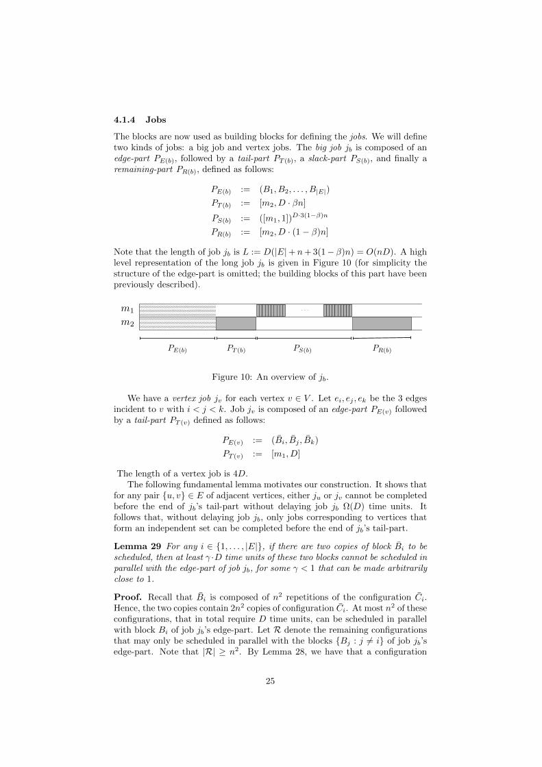
The blocks are now used as building blocks for defining the jobs. We will definetwo kinds of jobs: a big job and vertex jobs. The big job jb is composed of anedge-part PE(b), followed by a tail-part PT (b), a slack-part PS(b), and finally aremaining-part PR(b), defined as follows:

PE(b) := (B1, B2, . . . , B|E|)

PT (b) := [m2, D · βn]

PS(b) := ([m1, 1])D·3(1−β)n

PR(b) := [m2, D · (1− β)n]

Note that the length of job jb is L := D(|E|+ n+ 3(1− β)n) = O(nD). A highlevel representation of the long job jb is given in Figure 10 (for simplicity thestructure of the edge-part is omitted; the building blocks of this part have beenpreviously described).

m1

m2

PE(b) PT (b) PS(b) PR(b)

Figure 10: An overview of jb.

We have a vertex job jv for each vertex v ∈ V . Let ei, ej , ek be the 3 edgesincident to v with i < j < k. Job jv is composed of an edge-part PE(v) followedby a tail-part PT (v) defined as follows:

PE(v) := (Bi, Bj , Bk)

PT (v) := [m1, D]

The length of a vertex job is 4D.The following fundamental lemma motivates our construction. It shows that

for any pair u, v ∈ E of adjacent vertices, either ju or jv cannot be completedbefore the end of jb’s tail-part without delaying job jb Ω(D) time units. Itfollows that, without delaying job jb, only jobs corresponding to vertices thatform an independent set can be completed before the end of jb’s tail-part.

Lemma 29 For any i ∈ 1, . . . , |E|, if there are two copies of block Bi to bescheduled, then at least γ ·D time units of these two blocks cannot be scheduled inparallel with the edge-part of job jb, for some γ < 1 that can be made arbitrarilyclose to 1.

Proof. Recall that Bi is composed of n2 repetitions of the configuration Ci.Hence, the two copies contain 2n2 copies of configuration Ci. At most n2 of theseconfigurations, that in total require D time units, can be scheduled in parallelwith block Bi of job jb’s edge-part. Let R denote the remaining configurationsthat may only be scheduled in parallel with the blocks Bj : j 6= i of job jb’sedge-part. Note that |R| ≥ n2. By Lemma 28, we have that a configuration

25

Ci can be scheduled in parallel with a block Bj , with i 6= j, during at mostεn4d log n time units, for an arbitrarily small constant ε > 0. As the edge-partof jb consists of |E| = 3n/2 blocks, |R| ≥ n2, and configurations belongingto a job must be scheduled in a fixed order, almost all configurations in R arescheduled in parallel with at most one block of job jb’s edge-part. It follows thatat most D+n2 ·n4d log nε = D(1+ ε) time units of the two copies (requiring 2Dtime units in total) can be scheduled in parallel with job jb’s edge-part, whereε > 0 can be made an arbitrarily small constant.

4.1.5 The Two Machines Analysis

The intuition of the analysis is depicted in Figure 11 (for simplicity only blocksare depicted and not their operations).

m1

m2

PE(b) PT (b) PS(b) PR(b)

. . . . . .B1 B2 B4. . .

B1 B2 B4. . . . . .

. . .

Figure 11: Structure of a schedule that does not delay the completion time ofthe big job jb (depicted in light gray). The vertex jobs are depicted in a darkergray with one of them highlighted (in slightly lighter dark gray). As a blockBj of a vertex job only can be scheduled in parallel with either the block Bjor the slack-part of jb, the vertex jobs that complete before the slack-part of jbform an independent set. From that it follows that the number of vertex jobsthat need to be scheduled in parallel with the slack- and remaining-parts of jbdepends on the size of a maximum independent set of the given graph whichyields the desired gap.

Completeness: We will see that if graph G has an independent set of size βnthen all vertex jobs can be scheduled in parallel with the big job jb. Thus themakespan of the schedule will equal L (the length of job jb).

Let V ′ ⊆ V denote an independent set of G with |V ′| = βn. Since V ′ formsan independent set no two vertices in V ′ are incident to the same edge. Thus,the edge-parts PE(v) and PE(u) for two different nodes v, u ∈ V ′ do not containany common block. Recall that a block Bi can be scheduled in parallel witha block Bi, the tail-part of a vertex job requires time D on machine m1 andthe tail-part PT (b) of jb requires time Dβn on machine m2. It follows that thevertex jobs corresponding to the vertices in V ′ can all be scheduled in parallelwith the edge-part PE(b) = (B1, B2, . . . , B|E|) and the tail-part PT (b) of jb. As(i) the slack-part of job jb consists of D · 3(1− β)n unit time operations on m1,(ii) a block Bi can be scheduled in parallel with D slack-operations, and (iii) theremaining-part of job jb consists of one operation on machine m2 that requirestime D(1 − β)n, the (1 − β)n jobs corresponding to the vertices of V \ V ′ canbe scheduled in parallel with the slack-part and remaining-part of jb.

Soundness: As the makespan equals L — the length of job jb — in thecompleteness case, we will analyze the soundness case by showing that there is

26

a fraction of the operations belonging to the vertex jobs that are not scheduledin parallel with jb. Then it follows that if graph G has no independent set ofsize αn then the length of any schedule is at least (1 + Ω(1))L.

For any given schedule, let t1 be the time at which the tail-part PT (b) of jb iscompleted, and t2 the time at which the remaining-part PR(b) of jb starts. LetT := n · D denote the sum of the lengths of tail-parts of the vertex jobs. Letτ1,τ2 and τ3 be the fraction of T spent to schedule tail-operations of the vertexjobs during time interval [0, t1), [t1, t2) and [t2,∞), respectively.

It is easy to observe that any positive value of τ2 implies that τ2 · T timeunits are not scheduled in parallel with job jb. Similarly a positive value of τ3implies that max0, (τ3 − (1 − β))T time units are not scheduled in parallelwith jb. Finally, note that there are at least τ1 ·n vertex jobs that complete theiredge-part before time t1. Since G has no independent set of size αn, it followsthat there are at least max0, (τ1 − α)n conflicting pairs of vertex jobs (i.e.,corresponding to adjacent pairs of vertices). There are thus two “conflicting”copies of max0, (τ1 − α)n different blocks from Bi : i = 1, . . . , |E| to bescheduled before time t1. By using Lemma 29, we can easily check that at least(τ1 − α)n · γ · D time units of these conflicting blocks cannot be scheduled inparallel with job jb.

By the above arguments, it follows that the makespan of the schedule isat least the length of job jb plus (β − α)γ · n · D, where γ < 1 can be madearbitrarily close to 1. Hence, as L = O(nD), the length of any schedule in thesoundness case is at least (1 + Ω(1))L.

4.2 The Preemptive Three Machines Case

In the following we consider the preemptive three machines case and proveTheorem 6. We show that problem J3|pmtn|Cmax has no PTAS by presentinga gap-preserving reduction from the NP-hard problem to distinguish betweenn-vertex cubic graphs that have an independent set of size β · n and thosethat have no independent set of size α · n, for some β > α (see Theorem 9).In the reduction, the nodes of the cubic graph are mapped to jobs that areconstructed as a concatenation of “well-structured” sequences. The definitionand the analysis of these sequences are the arguments of the next subsections.The jobs will be defined subsequently.

In the following we will use several times a well-known property that ensuresthat there exists an optimal schedule for the preemptive job shop problem wherepreemptions occur at integral times [3].

4.2.1 Sequences

Let d = O(log n), for each frequency f = 1, . . . , d, we define four basic sequencesof operations:

Sx,f :=(

[mx, n4(d−f+1)], [mx+1, n

4(d−f+1)])n4f

Sx,f :=(

[mx+1, n4(d−f+1)], [mx, n

4(d−f+1)])n4f

for x ∈ 1, 2.

27

m1

m2

m1

m2

m1

m2

m1

m2

(b)

(c)(a)

S1,j

S1,i

Figure 12: Two sequences with different frequencies with j > i.

Note that all sequences have the same length, `s := 2n4(d+1), and Sx,f canbe scheduled in parallel with Sx,f , for x ∈ 1, 2 and f = 1, . . . , d.

The following lemma will be used several times. Informally, it says that iffor “many” time units a sequence is scheduled in parallel with a lower frequencysequence, then the completion time of the latter is larger than its length by“many” time units. (Figure (12-b) shows that only a “small” fraction of anygiven sequence can be scheduled in parallel with another sequence having lowerfrequency, and without delaying the latter; Figure (12-c) shows that any addi-tional time unit spent in parallel would delay the lower frequency sequence bythe same amount).

Lemma 30 For any j > i, consider a schedule for Sx,j and Sx,i, where x ∈1, 2. If there are t time units where sequences Sx,j and Sx,i are scheduled inparallel, then the time required to complete Sx,i is at least `s + t− o

(`s/n

3).

Proof. Consider a single operation O of Sx,i that requires n4(d−i+1) time unitson machine mx. As Sx,j has an operation on machine mx between any twoconsequent operations on machine mx+1, at most one operation of Sx,j (thatrequires n4(d−j+1) time units) can overlap O without interrupting it. Moreover,if, for some c > 1, c · n4(d−j+1) time units of Sx,j is scheduled in parallel with

O, then operation O must have been interrupted by at least d c·n4(d−j+1)

n4(d−j+1) e − 1 =

dc − 1e operations of Sx,j , that in total requires dc − 1e · n4(d−j+1) additionaltime units. As Sx,i has 2n4i operations in total and j > i, Sx,j can be scheduledin parallel with Sx,i during at most 2n4i · n4(d−j+1) ≤ `s/n

4 = o(`s/n3) time

units without delaying Sx,i and any additional time units spent in parallel willdelay Sx,i with at least the same amount.

4.2.2 Types

For each f = 1, . . . d, we define type Tf and Tf as follows:

Tf :=(S1,f , S2,(d−f+1)

)n4

Tf :=(S1,f , S2,(d−f+1)

)n4

28

Additionally, we define an extra type T0 as a sequence of 2n4 “long” opera-tions on machines m3 and m1 (this type will be part of the long job jb definedlater):

T0 := (S3,0, S1,0)n4

S3,0 := [m3, `s]

S1,0 := [m1, `s]

The total length of a type is `T := 2n4`s. Note that the operations of T0 can bescheduled in parallel with those of Tf and Tf , for f = 1, . . . , d, and completedby time `T .

We additionally observe that if T0 and Tf (Tf ) are completed by time `T ,then at any point of time interval [0, `T ], either an occurrence of S1,0, or S1,f

(or S1,f ) are processed (similarly, S3,0, or S2,(d−f+1) (or S2,(d−f+1))). Moreover,this structural property cannot be violated “many” times without increasing thecompletion time of either T0, or Tf (Tf ), by “many” time units.

Definition 31 For any given Tf (Tf ) with f = 1, . . . , d, we say that Tf ( Tf )is not alternated with T0 for t time units if at least one of the following twosituations happens:

1. There are t units where neither an occurrence of S1,0 nor an occurrenceof S1,f (S1,f ) is processed.

2. There are t units where neither an occurrence of S3,0 nor an occurrenceof S2,(d−f+1) (S2,(d−f+1)) is processed.

Lemma 32 Consider any feasible schedule for T0 and Tf (Tf ) and let Cmaxbe the completion time of the last operation. If for t units within time interval[0, Cmax] Tf (Tf ) is not alternated with T0, then Cmax ≥ `T + Ω(t)− o(`T /n3).

Proof. We provide the proof when Tf is not alternated with T0 for t time unitsbecause there are t units where, neither an occurrence of S1,0, nor an occurrenceof S1,f is processed (the other cases are similar).

Let t1 be the total time units where either an occurrence of S1,0 or anoccurrence of S1,f , but not both, is executed. Let t2 be the total time unitswhere occurrences of both, S1,0 and S1,f , are executed in parallel. Note that`T = t1 + 2 · t2, and therefore

Cmax ≥ t+ t1 + t2 = t+ `T − t2 (1)

If, for some c > 1, c ·n4(d−f+1) time units of an occurrence S1,f is scheduledin parallel with an occurrence O of S1,0, then operation O must have been

interrupted by at least d c·n4(d−f+1)

n4(d−f+1) e − 1 = dc − 1e operations of S1,f ; This

situation increases the completion time of T0 by dc−1e·n4(d−f+1) additional timeunits. As T0 has n4 occurrences of S1,0, S1,f can be scheduled in parallel with theoccurrences of S1,0 during at most n4 · n4(d−f+1) ≤ n4(d+1) = `s/2 = o(`T /n

3)time units without delaying T0, and any additional time units spent in parallelwill delay T0 by at least the same amount. The latter means that

Cmax ≥ `T + t2 − o(`T /n3) (2)

29

By summing inequalities (1) and (2), we conclude that Cmax ≥ `T + t/2 −o(`T /n

3), and the claim follows.The following lemma shows that only a small fraction of a type Tj can be

scheduled in parallel with Tk without delaying the completion time of T0 or Tk,whenever j 6= k. For an intuition see Figure 13.

m2

m3

S2,k

S1,k

m1

......

...

m2

m3

S1,j S2,j

m1

S1,j S2,j

.........

...

S1,j S2,j

S1,k S1,k

S2,k S2,k

(a)

(b)

Figure 13: Different types. The dark gray operations in (a) belong to typeT0 and can be scheduled in parallel with type Tk. In (b) the operations of Tjare depicted and Lemma 33 says that these operations cannot be scheduled inparallel with types Tk and T0, depicted in (a), without delaying one of them.

Lemma 33 For j 6= k, consider a schedule of Tj , Tk, and T0. If Tj is scheduledin parallel with Tk during t time units then the completion time of either Tk orT0 is at least `T + Ω(t)− o

(`T /n

3).

Proof. Recall that Tj =(S1,j , S2,(d−j+1)

)n4

and Tk =(S1,k, S2,(d−k+1)

)n4

. Wehave that either j > k or d− j+1 > d−k+1. We assume the former inequality(the other case is symmetric).

By Lemma 32, we assume that the amount of time units t0 where neitherS1,0, nor S1,k are processed is “much smaller” than t, namely t0 = o(t), otherwisethe claim follows.

Then by Lemma 30, a sequence S1,j can be scheduled in parallel with asequence S1,k during at most o(`s/n

3) time units without increasing the timeneeded to complete S1,k and any additional time units spent in parallel increasesthe time needed of the same amount. Since Tk has n4 occurrences of S1,k wehave that if the occurrences of Si,j are scheduled in parallel with the occurrencesof S1,k, during t time units, then Tk has completion time that is smaller thanits length plus t, namely `t + t, by at most o( `sn3 · n4) units. It follows that Tkhas completion time at least `T + Ω(t)− o(n · `s) = `T + Ω(t)− o(`T /n3) (recallthat `T = 2n4`s).

30

Moreover by a similar argument, if the occurrences of S1,j are scheduled inparallel with the occurrences S1,0, during t time units, then, during at leastΩ(t)− o(`T /n3) time units T0 cannot be scheduled.

The statement now follows by observing that every second sequence of Tjis an occurrence of S1,j and hence if Tj is scheduled in parallel with Tk duringt > `T /n

4 time units, then Ω(t) time units of the occurrences of S1,j mustbe scheduled. By the above arguments this would cause either T0 or Tk to beinterrupted during at least Ω(t)− o(`T /n3) time units.

4.2.3 Configurations and Blocks

For i = 1, . . . , |E|, a configuration Ci = (Tπi,1 , . . . , Tπi,logn) is an ordered se-

quence of log n types, where πi,j ∈ 1, . . . , d denotes the frequency of the j-thtype of configuration Ci. Lemma 26 shows that we can define a set of configu-rations C = Ci : i = 1, . . . , |E| such that any two configurations Ci ∈ C andCj ∈ C with i 6= j have at most ε log n types in common, for ε > 0 arbitrarilysmall. The set C = Ci : i = 1, . . . , |E| is defined in a similar way by using thetypes Ti, i.e., for i = 1, . . . , |E| we have Ci = (Tπi,1 , . . . , Tπi,logn

)We are now ready to define the different blocks. For i = 1, . . . , |E|, block

Bi is obtained by concatenating Ci for n2-times, i.e. Bi := (Ci)n2

; similarly

Bi := (Ci)n2

. Additionally, we define an extra configuration C0 := (T0)logn and

a corresponding block B0 := (C0)n2

.The length of any block is D := `T ·n2 log n. Moreover, the operations of B0

can always be scheduled in parallel with those of Bi and Bi, for i = 1, . . . , |E|.Therefore the blocks B0, Bi, and Bi, for i = 1, . . . , |E| can be completed by timeD. However, only a small fraction of a block Bi can be scheduled in parallelwith Bj without delaying the completion time of B0 or Bj , whenever i 6= j.

Lemma 34 For i 6= j, consider a schedule of Bi, Bj, and B0. If Bi is scheduledin parallel with Bj during t time units then the completion time of either Bj orB0 is at least D + Ω(t)− o(D/n1.5).

Proof. The block Bi is composed of n2 repetitions of Ci (consisting of log ntypes) and the block Bj is composed of n2 repetitions of Cj . Moreover, outof Bi’s sequence of n2 log n types there is a subset A of at least (1 − ε)n2 log ntypes so that if Tk ∈ A then the sequence Bi has no occurrence of Tk. ByLemma 33 together with that Bj is a sequence of n2 log n types and B0 isn2 log n repetitions of T0, we have that if t time units of the types in A arescheduled in parallel with Bj then either Bj or B0 has completion time at leastD+Ω(t)−o(n2 log n ·`T /n3) = D+Ω(t)−o(D/n3) (recall that D = `Tn

2 log n).The statement now follows from observing that if t > D/n1.5 time units of Bihave been scheduled then Ω(t) time units of the types in A have been scheduled.

The remaining part of the construction has several similarities with the 2-machines case.

4.2.4 Jobs

There are two long jobs, ja and jb. Job ja is composed of an edge-part PE(a),followed by a tail-part PT (a), a slack-part PS(a), and finally a remaining-partPR(a) defined as follows:

31

PE(a) :=(B1, B2, . . . , B|E|

)PT (a) := ([m1, 1], [m2, 1])

βnD2

PS(a) :=([m1, n

4], [m2, n4], [m3, n

4]) 3(1−β)nD

n4

PR(a) := ([m1, 1], [m2, 1])(1−β)nD

2

Similarly, job jb is composed of an edge-part PE(b), followed by a tail-part PT (b),a slack-part PS(b), and finally a remaining-part PR(b) defined as follows:

PE(b) := (B0)|E|

PT (b) := ([m2, 1], [m3, 1])βnD

2

PS(b) :=([m2, n

4], [m3, n4], [m1, n

4]) 3(1−β)nD

n4

PR(b) := ([m2, 1], [m3, 1])(1−β)nD

2

In Section 4.2.3 we observed that the operations of B0 can always be scheduledin parallel with those of Bi, for i = 1, . . . , |E|. Thus, the edge-parts PE(a) andPE(b) of jobs ja and jb can be scheduled in parallel. Clearly, the same appliesto the other parts. It follows that long jobs can be scheduled in parallel and thelength of both is

L := (|E|+ n+ 9(1− β)n)D = O(nD) (3)

A high level representation of the long jobs is given in Figure 14, where theoperations of ja and jb are colored in white and gray, respectively (for simplicitythe structure of the edge part is omitted, the structure of this part is discussedin Section 4.2.3 ).

m2

m3

m1

...

...

.........

...

...

...

...

BT BS BR

1 1

BE

n4

Figure 14: Long jobs.

We have a vertex job jv for each vertex v ∈ V . Let ei, ej , ek be the threeedges incident to v with i < j < k. Job jv is composed of an edge-part PE(v)

followed by a tail-part PT (v) defined as follows:

PE(v) :=(Bi, Bj , Bk

)PT (v) := ([m3, 1], [m1, 1])

D2

The length of any vertex job is 4D.

32

The following fundamental lemma motivates our construction. It shows thatthe jobs corresponding to adjacent vertices cannot be completed before the endof ja’s tail-part in the schedule without delaying either ja or jb. It follows that,without delaying job ja or jb, only jobs corresponding to vertices that form anindependent set can be completed before job ja’s tail-part.

Lemma 35 For I ⊆ 1, . . . , |E|, consider a schedule of two copies of eachblock in Bii∈I together with ja and jb. If the copies of Bii∈I are scheduledin parallel with PE(a) during |I| ·D + t time units then the completion time ofeither ja or jb is at least L+ Ω(t)− o(D).

Proof. Consider a fixed i ∈ I. Clearly, as block Bi requires D time units, wecan schedule at most D time units of the two blocks Bi in parallel with blockBi. By Lemma 34, if t time units of Bi is scheduled in parallel with any Bh,for h = 1, . . . , |E| and h 6= i, then either Bh (belonging to ja) or a block B0

(belonging to jb) is interrupted during at least Ω(t)− o(D/n1.5) time units. Itfollows that if D+ t time units of the two copies of Bi are scheduled in parallelwith PE(a) then, as PE(a) consists of 3n/2 blocks, either job ja or job jb areinterrupted during Ω(t)− o(3n/2 ·D/n1.5) = Ω(t)− o(D) time units.

By observing that the copies of Bii∈I can be scheduled in parallel duringvery few time units, we have that if |I| ·D+ t time units of the copies of Bii∈Iare scheduled in parallel with PE(a) then either job ja or jb are interruptedduring Ω(t)− o(D) time units.

4.2.5 The Three Machines Unit Time Analysis

Completeness: We will see that if graph G has an independent set of sizeβn then all vertex jobs can be scheduled in parallel with the long jobs. Themakespan of the resulting schedule will be equal to (3).

Long jobs are scheduled to complete at time L (3) (see, e.g., Figure 14).Let V ′ ⊆ V denote an independent set of G with |V ′| = βn. Since V ′ formsan independent set no two vertices in V ′ are incident to the same edge. Fori = 1, . . . , |E|, observe that block Bi can be scheduled in parallel with block Bi.Moreover, we can schedule all the sequences from PT (v) : v ∈ V ′ in parallelwith PT (a) and PT (b). It follows that all the vertex jobs corresponding to thevertices in V ′ can be scheduled in parallel with the operations of long jobs fromblocks PE(a), PT (a), PE(b), PT (b).

The operations from PE(v) : v ∈ V \ V ′ can be scheduled in parallel withthe operations from PS(a), PS(b) without delaying or interrupting the executionof the slack parts of the long jobs (only the vertex job is preempted). Indeed,the total length of the operations in PE(v) : v ∈ V \V ′ is at most 3(1−β)nD,and each of these operations has length at least n4. Moreover, the length of theslack-part of the long jobs is 9(1− β)nD and note that in the slack-part of thelong jobs, during every 3n4 time units that are spent to process operations fromPS(a), PS(b), we can schedule at least n4 time units of an unscheduled operationfrom PE(v) : v ∈ V \ V ′, i.e. n4 time units are contiguously available on eachmachine (see Figure 14).

Finally, the remaining operations from the (1 − β)n tail-parts PT (v) : v ∈V \V ′, that in total require (1−β)nD time units, can be scheduled in parallelwith PR(a) and PR(b) (recall that both PR(a) and PR(b) require (1− β)nD timeunits).

33

Soundness: We show the existence of a gap by proving that if the graphhas no independent set of size αn then the length of any schedule is at leastL+ Ω(nD) = (1 + Ω(1))L.

For any given schedule, let t1 be the time at which operations from blocksPT (a) and PT (b) are completed. Let t2 be the time at which the first operationfrom PR(a) and PR(b) starts. Let τ1,τ2 and τ3 be the fraction of T = n ·D spentto schedule operations in PT (v) : v ∈ V during time interval [0, t1), [t1, t2) and[t2,∞), respectively. We consider the following cases.

(Case 1) τ1 = α+ c where c = Ω(1) is a positive constant;

(Case 2) τ2 = Ω(1) is a positive constant;

(Case 3) c = o(1) and τ2 = o(1).

For any 0 ≤ τ1 ≤ 1, note that there are at least τ1·n vertex jobs that completetheir edge part before time t1. In (Case 1), since G has no independent set ofsize αn, there are at least (τ1 − α)n = c · n = Ω(n) conflicting pairs of jobs(i.e., corresponding to edges of adjacent pairs of vertices). It follows that thereare two “conflicting” copies of Ω(n) different blocks from Bi : i = 1, . . . , |E|to be scheduled before time t1. Let t0 be the time the last operation fromblocks PE(a) and PE(b) is completed. Observe that t0 cannot be larger than|E|D+o(nD), otherwise we would be done since this would create a schedule oflength L+ Ω(nD). For the same reason, we can assume that t1 = L1 + o(nD),where L1 denotes the total length of the sequence (PE(a), PT (a)). It followsthat in time interval [t0, t1], machine m2 is occupied for t1 − t0 − o(nD) timeunits, by operations of the tail-part of long jobs. By these observations and byusing Lemma 35, we have that at least Ω(nD) time units of these conflictingblocks cannot be scheduled within time t1 without creating a schedule of lengthL+ Ω(nD).

Now, let us consider (Case 2). Remember that we can assume that t1 =L1+o(nD), otherwise we are done. The latter assumption implies that “almost”all operations from PS(a), PS(b), i.e. all but o(nD), are not yet scheduled attime t1. Let T12 be the set of operations from PT (v) : v ∈ V that are scheduledduring [t1, t2). Under (Case 2), we have that t2 − t1 = Ω(nD). Moreover wecan assume that with the exception of o(nD) time units, at every time point ininterval [t1, t2] an operation from PS(a), PS(b) is executed. Note that sequencesfrom PT (v) : v ∈ V have higher frequency than those in PS(a), PS(b). Byusing similar arguments as in the proof of Lemma 30, it is easy to check thatwithout delaying the long jobs we can only schedule a tiny fraction of T12, i.e.at most o(nD) time units. Moreover, additional time units of operations fromT12 can be processed in parallel with a long job only if a long job is delayedby at least the same amount. Under (Case 2), this implies a schedule of lengthL+ Ω(nD).

Finally, in (Case 3), we have τ1 + τ2 = α + o(1) and therefore τ3 = 1 −α − o(1) > 1 − β. This means that we have to schedule (β − α − o(1))nDtime units more than the space available to finish by time (3) (recall that thelengths of PR(a) and PR(b) are both (1 − β)nD). This creates a schedule oflength L+ Ω(nD).

34

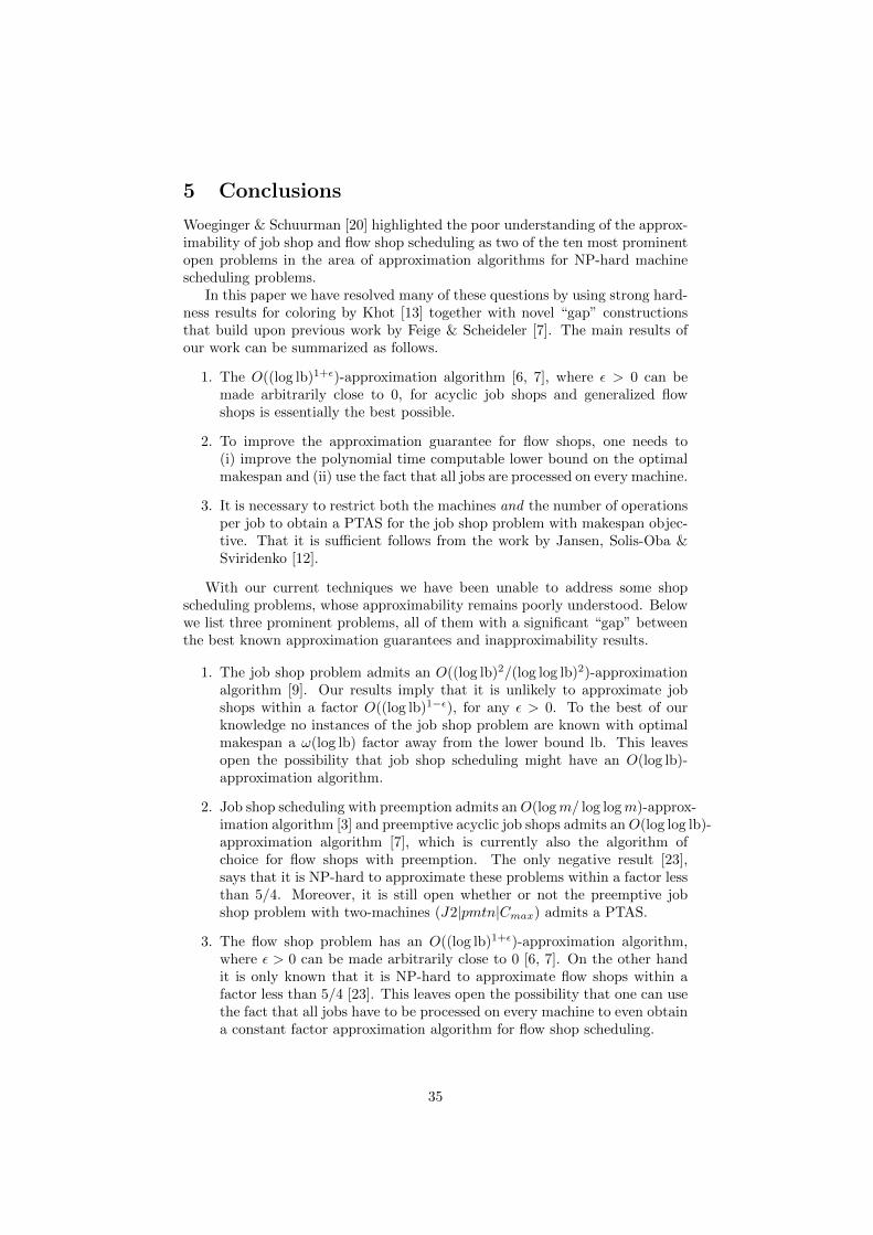
5 Conclusions

Woeginger & Schuurman [20] highlighted the poor understanding of the approx-imability of job shop and flow shop scheduling as two of the ten most prominentopen problems in the area of approximation algorithms for NP-hard machinescheduling problems.

In this paper we have resolved many of these questions by using strong hard-ness results for coloring by Khot [13] together with novel “gap” constructionsthat build upon previous work by Feige & Scheideler [7]. The main results ofour work can be summarized as follows.

1. The O((log lb)1+ε)-approximation algorithm [6, 7], where ε > 0 can bemade arbitrarily close to 0, for acyclic job shops and generalized flowshops is essentially the best possible.

2. To improve the approximation guarantee for flow shops, one needs to(i) improve the polynomial time computable lower bound on the optimalmakespan and (ii) use the fact that all jobs are processed on every machine.

3. It is necessary to restrict both the machines and the number of operationsper job to obtain a PTAS for the job shop problem with makespan objec-tive. That it is sufficient follows from the work by Jansen, Solis-Oba &Sviridenko [12].

With our current techniques we have been unable to address some shopscheduling problems, whose approximability remains poorly understood. Belowwe list three prominent problems, all of them with a significant “gap” betweenthe best known approximation guarantees and inapproximability results.

1. The job shop problem admits an O((log lb)2/(log log lb)2)-approximationalgorithm [9]. Our results imply that it is unlikely to approximate jobshops within a factor O((log lb)1−ε), for any ε > 0. To the best of ourknowledge no instances of the job shop problem are known with optimalmakespan a ω(log lb) factor away from the lower bound lb. This leavesopen the possibility that job shop scheduling might have an O(log lb)-approximation algorithm.

2. Job shop scheduling with preemption admits anO(logm/ log logm)-approx-imation algorithm [3] and preemptive acyclic job shops admits anO(log log lb)-approximation algorithm [7], which is currently also the algorithm ofchoice for flow shops with preemption. The only negative result [23],says that it is NP-hard to approximate these problems within a factor lessthan 5/4. Moreover, it is still open whether or not the preemptive jobshop problem with two-machines (J2|pmtn|Cmax) admits a PTAS.

3. The flow shop problem has an O((log lb)1+ε)-approximation algorithm,where ε > 0 can be made arbitrarily close to 0 [6, 7]. On the other handit is only known that it is NP-hard to approximate flow shops within afactor less than 5/4 [23]. This leaves open the possibility that one can usethe fact that all jobs have to be processed on every machine to even obtaina constant factor approximation algorithm for flow shop scheduling.

35

Acknowledgments. We are grateful to Maxim Sviridenko who introduced usto the problem and gave useful references. Also, many thanks to Subhash Khotfor a kind explanation of his results.

This research is supported by Swiss National Science Foundation project N.200020-122110/1 “Approximation Algorithms for Machine Scheduling ThroughTheory and Experiments III” and by Hasler Foundation Grant 11099. Thesecond author is also supported by ERC Advanced Investigator Grant 226203.

The first author would like to dedicate this work to Edoardo on the occasionof his birth.

References

[1] P. Alimonti and V. Kann. Some APX-completeness results for cubic graphs.Theoretical Computer Science, 237(1-2):123–134, 2000.

[2] E. J. Anderson, T. S. Jayram, and T. Kimbrel. Tighter bounds on pre-emptive job shop scheduling with two machines. Computing, 67(1):83–90,2001.

[3] N. Bansal, T. Kimbrel, and M. Sviridenko. Job shop scheduling with unitprocessing times. Mathematics of Operations Research, 31:381–389, 2006.

[4] J. Beck. An algorithmic approach to the lovasz local lemma. RandomStructures and Algorithms, 2(4):343–365, 1991.

[5] B. Chen, C. N. Potts, and G. J. Woeginger. A review of machine scheduling:Complexity, algorithms and approximability. Handbook of CombinatorialOptimization, 3:21–169, 1998.

[6] A. Czumaj and C. Scheideler. A new algorithm approach to the generallovasz local lemma with applications to scheduling and satisfiability prob-lems (extended abstract). In Proceedings of the 32nd Annual ACM Sym-posium on Theory of Computing (STOC), pages 38–47, 2000.

[7] U. Feige and C. Scheideler. Improved bounds for acyclic job shop schedul-ing. Combinatorica, 22(3):361–399, 2002.

[8] A. V. Fishkin, K. Jansen, and M. Mastrolilli. Grouping techniques forscheduling problems: Simpler and faster. Algorithmica, 51(2):183–199,2008.

[9] L. A. Goldberg, M. Paterson, A. Srinivasan, and E. Sweedyk. Better ap-proximation guarantees for job-shop scheduling. SIAM Journal on DiscreteMathematics, 14(1):67–92, 2001.

[10] R. Graham, E. Lawler, J. Lenstra, and A. R. Kan. Optimization and ap-proximation in deterministic sequencing and scheduling: A survey. Annalsof Discrete Mathematics, 5:287–326, 1979.

[11] H. Hoogeveen, P. Schuurman, and G. J. Woeginger. Non-approximabilityresults for scheduling problems with minsum criteria. INFORMS Journalon Computing, 13(2):157–168, 2001.

36

[12] K. Jansen, R. Solis-Oba, and M. Sviridenko. Makespan minimization injob shops: A linear time approximation scheme. SIAM Journal on DiscreteMathematics, 16(2):288–300, 2003.

[13] S. Khot. Improved inapproximability results for maxclique, chromatic num-ber and approximate graph coloring. In Proceedings of the 42nd AnnualSymposium on Foundations of Computer Science (FOCS), pages 600–609,2001.

[14] E. L. Lawler, J. Lenstra, A. R. Kan, and D. Shmoys. Sequencing andscheduling: Algorithms and complexity. Handbook in Operations Researchand Management Science, 4:445–522, 1993.

[15] F. T. Leighton, B. M. Maggs, and S. B. Rao. Packet routing and job-shopscheduling in O(congestion + dilation) steps. Combinatorica, 14(2):167–180, 1994.

[16] F. T. Leighton, B. M. Maggs, and A. W. Richa. Fast algorithms for findingO(congestion + dilation) packet routing schedules. Combinatorica, 19:375–401, 1999.

[17] V. Nagarajan and M. Sviridenko. Tight bounds for permutation flow shopscheduling. In Proceedings of the 13th Conference on Integer Programmingand Combinatorial Optimization (IPCO), pages 154–168, 2008.

[18] C. Potts, D. Shmoys, and D. Williamson. Permutation vs. nonpermutationflow shop schedules. Operations Research Letters, 10:281–284, 1991.

[19] M. Queyranne and M. Sviridenko. Approximation algorithms for shopscheduling problems with minsum objective. Journal of Scheduling,5(4):287–305, 2002.

[20] P. Schuurman and G. J. Woeginger. Polynomial time approximation algo-rithms for machine scheduling: ten open problems. Journal of Scheduling,2(5):203–213, 1999.

[21] S. V. Sevastianov and G. J. Woeginger. Makespan minimization in pre-emptive two machine job shops. Computing, 60(1):73–80, 1998.

[22] D. Shmoys, C. Stein, and J. Wein. Improved approximation algorithms forshop scheduling problems. SIAM Journal on Computing, 23:617–632, 1994.

[23] D. P. Williamson, L. A. Hall, J. A. Hoogeveen, C. A. J. Hurkens, J. K.Lenstra, S. V. Sevastianov, and D. B. Shmoys. Short shop schedules. Op-erations Research, 45:288–294, 1997.

37