Lower Level Mediation in Multilevel Modelsnb2229/docs/kenny-korchmaros-bolger-pm-2003.… · Lower Level Mediation in Multilevel Models David A. Kenny and ... tional states (e.g.,

Lower Level Mediation in Multilevel Models

David A. Kenny andJosephine D. Korchmaros

University of Connecticut

Niall BolgerNew York University

Multilevel models are increasingly used to estimate models for hierarchical andrepeated measures data. The authors discuss a model in which there is mediation atthe lower level and the mediational links vary randomly across upper level units.One repeated measures example is a case in which a person’s daily stressors affecthis or her coping efforts, which affect his or her mood, and both links vary ran-domly across persons. Where there is mediation at the lower level and the media-tional links vary randomly across upper level units, the formulas for the indirecteffect and its standard error must be modified to include the covariance between therandom effects. Because no standard method can estimate such a model, the authorsdeveloped an ad hoc method that is illustrated with real and simulated data. Limi-tations of this method and characteristics of an ideal method are discussed.

Multilevel models for hierarchical and repeatedmeasures data are becoming increasingly common(Diggle, Heagerty, Liang, & Zeger, 2001; Hox, 2002;Raudenbush & Bryk, 2002; Snijders & Bosker, 1999).These models assume that there are at least two levelsin a data set, an upper level, or Level 2, and a lowerlevel, or Level 1. The Level 1 units are nested withinthe Level 2 units. In some applications, the upperlevel refers to persons and the lower level refers toobservations or repeated measurements. For example,a researcher might collect daily diary (repeated mea-sures) data over several weeks on people’s exposureto daily stressors, their coping efforts, and their emo-tional states (e.g., Bolger, Davis, & Rafaeli, 2003;Bolger & Zuckerman, 1995). In other applications,the upper level refers to groups and the lower levelrefers to persons who are members of those groups.For example, a researcher may collect demographicbackground, parenting practices, and educationalachievement data on all schoolchildren in a sample ofschools (e.g., Raudenbush & Bryk, 1986). In this ex-

ample, schools are the groups, and schoolchildren arethe persons nested within those groups.

A basic multilevel model for the repeated measuresdata might specify that at Level 1, the repeated mea-sures level, a person’s mood on a given day is a func-tion of a baseline mood level that is common acrossall days, a stressor reactivity effect that reflectswhether or not he or she has experienced a stressorthat day, and a Level 1 residual effect that variesrandomly from day to day but whose average value iszero. At Level 2, the between-person level, the modelmight specify that people differ in how reactive theyare to daily stressors and that a given person’s reac-tivity is a function of an effect that is common to allpeople, and a residual Level 2 effect that varies ran-domly from person to person but whose average valueis zero.

Multilevel modeling has several advantages overtraditional models for such data. For instance, unliketraditional models for repeated measures data, multi-level models can effectively manage unequal groupsizes and missing data on the repeated measure. Mul-tilevel modeling can also be used to examine simul-taneously the effects of Level 2 (e.g., school level)and Level 1 (e.g., child level) variables in nested datasets. In doing so, multilevel models take account of(and adjust for) any bias in standard errors and statis-tical tests resulting from the nonindependence ofobservations that is typical in such data (Krull &MacKinnon, 2001). Because of these advantages andothers, multilevel modeling has drawn substantial at-tention recently.

David A. Kenny and Josephine D. Korchmaros, Depart-ment of Psychology, University of Connecticut; Niall Bol-ger, Department of Psychology, New York University.

This research was supported in part by National Instituteof Mental Health Grant RO1-MH51964 to David A. Kennyand Grant RO1-MH60366 to Niall Bolger.

Correspondence concerning this article should be ad-dressed to David A. Kenny, Department of Psychology,University of Connecticut, Storrs, Connecticut 06269-1020.E-mail: [email protected]

Psychological Methods Copyright 2003 by the American Psychological Association, Inc.2003, Vol. 8, No. 2, 115–128 1082-989X/03/$12.00 DOI: 10.1037/1082-989X.8.2.115

115

Testing mediational hypotheses is a central activityin psychological science (Baron & Kenny, 1986;Kenny, Kashy, & Bolger, 1998; Shrout & Bolger,2002), and mediational questions are as relevant tomultilevel data as they are to traditional data struc-tures. Kenny, Kashy, and Bolger (1998) introducedthe topic of multilevel mediation and explained thedistinction between upper level and lower level me-diation. In upper level mediation the initial or putativecausal variable whose effect is mediated is an upperlevel variable. An example of this type of mediation iswhere the effect of a school-level safer-sex interven-tion program (upper level initial variable) on students’intentions to engage in safer sex (lower level depen-dent variable) is mediated by students’ motivations toengage in safer sex (lower level mediator).

In lower level mediation, the initial variable is atthe lower level. In the repeated measures exampledescribed previously, this might be where the reactiv-ity effect of a daily stressor (lower level initial vari-able) on a person’s mood on a given day (lower leveldependent variable) is mediated by the person’s cop-ing efforts that day (lower level mediator). In theirdiscussion of lower level mediation, Kenny, Kashy,and Bolger (1998) considered cases where the lowerlevel initial variable and mediator show random upperlevel variability in their effects. This variability can bethought of as a form of moderation (Baron & Kenny,1986), a topic that we return to later. For instance, inthe repeated measures example, the effect of stressorson coping and the effect of coping on mood may varyacross persons, the upper level units. In prior workusing daily diary reports of stressors, coping, andmood, Bolger and Zuckerman (1995) found evidenceof random variability in these links.

Several researchers have focused on upper levelmediation. For example, Krull and MacKinnon (1999)described and evaluated methods used to test upperlevel mediated effects. Using both simulated and realdata, Krull and MacKinnon compared single level andmultilevel mediation analyses, two ways to calculatethe effect of the mediator, and two coefficient estima-tion methods, which coincided with the types of me-diation analyses. Raudenbush and Sampson (1999)also focused on upper level mediation. They demon-strated how the computer program HLM5 (Rauden-bush, Bryk, Cheong, & Congdon, 2000) can be usedto estimate and test upper level mediational models.Raudenbush and Sampson demonstrated this ap-proach using a multilevel design with latent variablesin which measurement error is represented as a level

within the model. Lastly, Krull and MacKinnon(2001) compared the appropriateness of single leveland multilevel data analysis procedures to test media-tion effects in nested data. Two of the three modelsthat they considered were upper level mediationalmodels.

By comparison, discussion of lower level media-tion in multilevel modeling has been sparse, and todate there has been no discussion of the case in whichthe mediational links show random upper level vari-ability. Judd, Kenny, and McClelland (2001) dis-cussed lower level mediational analysis but only inthe limited case where the problem could be recast interms of standard fixed-effects analysis of variance.Krull and MacKinnon (2001) also considered lowerlevel mediation in nested data but only to compare theappropriateness of single level and multilevel dataanalysis procedures to test a fixed-effects mediationalmodel.

Thus, although mediation in multilevel models hasbeen the focus of increasing attention recently, therehas been no discussion of analysis methods for caseswhere the putative causal variable is at the lowerlevel. As noted, with lower level mediation, all themediational links may vary randomly across the upperlevel units, and so, it is much more complicated thanupper level mediation. The present article provides acomplete overview of lower level mediational analy-sis in a fully random model using a multilevel frame-work, and it shows that interesting, unexpected, andimportant complications arise in this case.

The Lower Level Mediational Model

Consider a Level 1 variable, Y, that is assumed tobe caused by two other Level 1 variables, X and M. Ofkey interest in this article is the possibility that thevariable M may mediate the effect of X on Y, lowerlevel mediation. In this article, variable X is called theinitial or putative causal variable, M is the mediator,and Y is the outcome. Ideally X is a variable that isexperimentally manipulated, but it need not be. Forease of understanding, it might help to think of theexample given previously where X is the occurrenceof a stressor on a given day, M is the person’s copingefforts that day, and Y is the person’s mood that day.The upper level unit would be person, and the lowerlevel unit would be day.

Equations

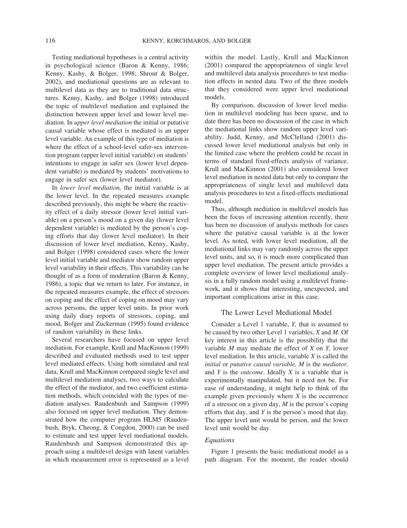
Figure 1 presents the basic mediational model as apath diagram. For the moment, the reader should

KENNY, KORCHMAROS, AND BOLGER116

ignore the subscripts in the coefficients. The variableX causes M, which in turn causes Y. For the example,stressors cause coping, which in turn causes mood.The direct effect of X on Y would be c�, and theindirect effect would be ab. The total effect, the directeffect plus indirect effect, would equal c� + ab, whichwe denote as c. The reader should note that we do notuse Greek letters for these effects, even though theyare population values. Whenever they are sample es-timates, we will make it clear.

In a multilevel model, lower level effects may varyby upper level unit. So, all of the effects, a, b, c�, andc might vary by the upper level unit. That is why theyare subscripted by the upper level unit, denoted inFigure 1 as j. The figure presents the mediationalmodel for upper level unit j. For the example, themediation of the stressor–mood relationship by cop-ing might vary by person, and so the direct effect ofstressor on mood, path cj�, might be different for dif-ferent persons.

More formally, we consider a two-level model inwhich the first subscript, i, refers to the lower level,and the second subscript, j, as in the figure, refers tothe upper level. The Level 1 equation for Y withoutthe mediator is

Yij � d0j + cjXij + rij. (1)

In this equation, Y is the outcome, d0j is the interceptfor each upper level unit, cj represents the effect of Xon Y for each upper level unit, and rij is an error term.The two mediational equations, implied in Figure 1,are

Mij = d1j + ajXij + eij (2)

and

Yij = d2j + cj�Xij + bjMij + fij. (3)

Equations 1, 2, and 3 are sometimes called the lowerlevel or Level 1 equations. We refer to path c (from

Equation 1) as the total effect of X on Y, path c�(Equation 3) as the direct effect, path a (Equation 2)as the effect of X on M, and path b (Equation 3) as theeffect of M on Y. All of these coefficients may varyacross the upper level units, which is why they eachhave the subscript j. The two intercepts in Equations2 and 3, denoted by d, are not central to our media-tional model.

The Level 2 equation for the total effect, whenthere are no Level 2 effects, is

cj � c + u0j , (4)

which simply says that the coefficient for unit j equalsthe average coefficient (the population mean) plus adeviation from that average for each upper level unit.So, c would represent the typical level of the totaleffect, and u0j would represent a deviation from thattypical level for upper level unit j. In the same way,we can write upper level equations for the other co-efficients in the lower level mediational model. Thefollowing are the upper level equations for the otherlower level coefficients when there are no Level 2effects:

aj = a + u1j, (5)

bj = b + u2j, (6)

and

cj� = c� + u3j. (7)

Thus, we denote the unsubscripted parameter as theaverage parameter value. (The intercepts also havesimilar Level 2 equations, but as noted, they are ir-relevant to our discussion.) Returning to the stressor–coping–mood example, we would allow for individualdifferences in the effect of stressors on mood (c andcj�; i.e., for some persons, stressors have more of aneffect on mood than for others). There might also beindividual differences in the effect of stressors on cop-ing (path a; i.e., a stressor might activate a copingstrategy for some persons but not for others). Finally,the effect of coping on mood (path b) might also varyby person (i.e., the coping strategy is effective forsome people but not for others).

Decomposition of Effects

The single level equation for the decomposition ofmediations effects (MacKinnon, Warsi, & Dwyer,1995) is

c � c� + ab. (8)

Figure 1. The Level 1 mediation model in which the effectof X on Y is partially mediated by M; for Level 2 unit j, Xcauses M (path aj), M causes Y (path bj), and X causes Y(path cj�).

MEDIATION IN MULTILEVEL MODELS 117

The equation states that the total effect (c) equals thedirect effect (c�) plus the indirect effect (ab). How-ever, Equation 8 presumes that a and b are fixed pa-rameters; that is, a and b do not vary across upper-level units.

If we assume that mediational effects a and b arerandom variables that have a bivariate normal distri-bution, a standard assumption within multilevel mod-eling, then it can be shown that the expected value ofajbj does not equal ab but rather equals ab + �ab

(Goodman, 1960). The expected value of a product orE(ajbj) does not equal the product of the expectedvalues of the components of that product or E(aj)E(bj)when aj and bj are correlated. Thus, given multivariatenormality, the total effect in fully random lower levelmediated multilevel models is decomposed as

c � c� + ab + �ab, (9)

where �ab is the population covariance of aj with bj

and refers to a possible correlation of aj and bj effects.A positive value for �ab implies that those upper levelunits that have large values of aj also have large val-ues of bj. Conversely, a negative value for �ab impliesthat those upper level units that have large values of aj

also have small values of bj. For the example, �ab

refers to the covariance between the effect of stressorson coping and the effect of coping on mood.

We should note that even if a and b were not ran-dom, then Equation 9 would not exactly hold for es-timates obtained from multilevel models (Krull &MacKinnon, 1999). Because maximum-likelihood es-timation, not ordinary least squares (OLS), is used,the equation is not exact, only approximate. Alterna-tively, we can avoid obtaining an independent esti-mate of the total effect c by instead estimating it in-directly by calculating c�, ab, and �ab and summingthem. Thus, the total effect would be defined as c� +ab + �ab.

In single level mediational analysis, the formula forthe sampling variance of the mediated effects, de-noted as �(ab)

2, is

�(ab)2 � b2�a

2 + a2�b2 + �a

2�b2. (10)

The formula for the variance of indirect effects givenby Sobel (1982) is an approximation and does notinclude the last term of the above equation (Aroian,1947; Baron & Kenny, 1986). Equation 10 presumesthat a and b are fixed; that is, they do not vary acrossupper level units. If, however, we presume that theseparameters are random, the equation for the variance

of mediated effects assuming multivariate normalityof effects is

�(ab)2 � b2�a

2 + a2�b2 + �a

2�b2 + 2ab�ab + �ab

2 (11)

(see Kendall & Stuart, 1958). The two terms in theright side of the equation that are not included in thesingle level formula (see Equation 10) involve �ab,the covariance of a and b, which is critical in theestimation and testing of lower level mediation inmultilevel models with random effects.

The variance of the total effect �c2, given the as-

sumption that all mediational links are random vari-ables whose joint distribution is multivariate nor-mal, is

�c2 � �c�

2 + b2�a2 + a2�b

2 + �a2�b

2 + 2ab�ab

+ �ab2 + 2b�ac� + 2a�bc�. (12)

Note that there are two new terms in this equation;one is the covariance between a and c� and the otheris the covariance between b and c�. We consider theterm �c

2 in more detail in the next section when wediscuss moderation.

Mediation and Moderation

In this section we consider both the mediation andmoderation of the effect of X on Y. We see that withmultilevel data in which both X and Y are Level 1variables, considerable detail can be obtained for bothmediation and moderation, much more than withsingle level models. For ease of presentation, we as-sume in this section that a, b, and c are all positive.

Controlling for M might reduce the overall effect ofX on Y (i.e., c). This is classical mediation. In the fullyrandom-effects multilevel model, there are two waysin which c� might be less than c. First, there is reduc-tion if ab is nonzero, or second, if �ab is nonzero.Note that ab might equal zero, but c� can still be lessthan c because �ab can be nonzero.

In the fully random-effects model, there is poten-tially Level 2 variation in the effect that X has on Y.This variation designated as �c

2 reflects evidence ofmoderation of the X-to-Y relationship, though theidentity of the moderating variable has yet to be dis-covered. We can also determine how much of thismoderation is reduced or even eliminated by control-ling for M. Note that if �c

2 were zero, then X wouldaffect Y to the same degree for all upper level units;that is, there would be no moderation. Stated differ-ently, if �c

2 equals zero, the effect of X on Y does notvary, and so, it does not make sense to search for


Level 2 factors that would explain any variation. Insummary, if the effect of X on Y is fully explained byM, then (a) the overall effect, c, should be explained,and c� would be zero, and (b) the variance of theeffects, �c

2, should be explained, and, therefore, �c�2

would be zero.For instance, assume that the population values are

a � 0.50, b � 1.00, and c� � 0.25. We set �a2 �

1.00, �b2 � 1.00, �c�

2 � 0.25, �ab � 0.50, and �ac�

� �bc� � 0.00. When we use the single level model(Equation 8), c � 0.25 + 0.50 � 0.75. Then, 67%, or(0.75 − 0.25)/0.75, of the overall effect of X on Y, or0.75, is mediated. However, using the formulas for afully random-effects model, it follows that c � 0.25+ 0.50 + 0.50 � 1.25 (Equation 9) and that �c

2 �0.25 + (1.00)2(1.00) + (0.50)2(1.00) + (1.00)(1.00) +2(0.50)(1.00)(0.50) + (0.50)2 + 2(1.00)(0.00) +2(0.50)(0.00) � 3.25 (Equation 12). Consequently, itis really that 80%, or (1.25 − 0.25)/1.25, of the overalleffect of X on Y, or 1.25, is mediated. It also followsthat 92% of the variance of the X-to-Y effect is ex-plained by variation in M, (3.25 − 0.25)/3.25. Theseproportions of the total effect, which in the currentexample are calculated using population values, illus-trate the importance of considering �ab when estimat-ing the amount of mediation in a fully random model.Note too that the correct value for �(ab)

2 would be3.00 as estimated by the formula for the fully random-effects model (Equation 11), not 2.25 as would beestimated using the single level formula (Equation10). The proportions of the total effect can also becalculated using sample estimates, though these pro-portions can be very unstable.

Even more surprising, consider the case where thepopulation values are a � 0.00, b � 0.00, c� � 0.00.In this model, there is no overall effect of X on Y,either direct or indirect. Using the single level modelformula (Equation 8), we would think that the totaleffect would have to be zero. However, it is not. If weset �a

2 � 1.00, �b2 � 1.00, or �c�

2 � 0.00, �ab �1.00, and �ac� � �bc� � 0.00, using the random ef-fects formulas, it follows that c � 0.00 + (0.00)(0.00)+ 1.00 � 1.00 (Equation 9) and that �c

2 � 2.00(Equation 12). Thus, we find that the total effect forthe average Level 2 unit is nonzero and is entirely dueto the covariance between a and b. To understand whythis is the case, we need to consider that in this ex-ample, although the average of a and the average of bboth equal zero, the average of ab tends to be positivebecause positive as are paired with positive bs andnegative as are paired with negative bs.

As the above examples illustrate, when �ab is thesame sign as ab and is not considered when determin-ing the amount of the mediation, the amount of me-diation is underestimated. However, when �ab is notconsidered, the amount of mediation could be over-estimated. This is the case when �ab is opposite insign to ab. Consider the following case: a � 0.50, b� 1.00, c� � 0.25, and �ab � −0.50. When we usethe single level approach (Equation 8), c � 0.25 +(0.50)(1.00) � 0.75. Then, 67%, or (0.75 − 0.25)/0.75, of the overall effect of X on Y, or 0.75, is me-diated. However, when we use the correct equationfor a random effects model (Equation 9), it followsthat c � 0.25 + (0.50)(1.00) − 0.50 � 0.25. Conse-quently, it is really that there is no mediation; that is,0%, (0.25 − 0.25)/0.25, of the overall effect of X on Y,or .25, is mediated.

The Substantive Meaning of the ab Covariance

The interpretation of �a2 and �b

2 is straightforward.The variance �a

2 represents differences in the effec-tiveness of X in causing the mediator M. The variance�b

2 represents differences in the effectiveness of M incausing the outcome Y. How might �ab be inter-preted? First, note that there must be some variation ina and b for there to be any covariance between thetwo. Such variation should be first established before�ab is interpreted.

The exact interpretation of �ab depends on the par-ticular application. Consider again the example of theeffect of stressors on mood. The mediator might be acoping style. It might be the case that the coping styleis more effective in relieving distress for some indi-viduals than for others and that variation is capturedby �b

2. For persons who have a large b (i.e., thecoping style is effective), it seems reasonable to ex-pect that stressors would induce more coping; there-fore, their a parameter would be large. By the sametoken, for those whose b path was small meaning thatthe coping style was ineffective, it is expected that thea path would be small indicating that stressors wouldnot affect amount of coping. Thus, it seems plausiblethat �ab would be positive and would be theoreticallyinteresting, although theoretical importance is not re-quired for consideration of �ab; the term �ab should beconsidered whenever decomposing the effects of alower level random-effects mediational model. If �ab

is the same sign as ab and is not considered, theamount of mediation would be underestimated.

It might also be the case that �ab is the opposite


sign of ab. Consider the case where ab is positive, and�ab is negative. For example, suppose that the effectof instruction quality (the degree to which the lessonis taught well) on a student’s learning is mediated bystudent motivation to learn. Overall, high quality in-struction leads to more motivation to learn, and moremotivation to learn leads to more learning. However,it might be the case that some students are extrinsi-cally motivated to learn and so are greatly affected byinstruction quality (i.e., their a parameter is large),whereas other students are intrinsically motivated andare not as affected by instruction quality (i.e., their aparameter is relatively small). This variation would becaptured by �a

2, which is the amount of variation inthe a parameter due to Level 2 unit, or in this case,participant. It may also be the case that the studentswho are extrinsically motivated to learn—have a largea parameter—have not developed good study skills.Consequently, an increase in their motivation to learnhas little impact on learning (i.e., their b parameter issmall). Conversely, students who are intrinsically mo-tivated to learn—have a small a parameter—have de-veloped their study skills, and consequently, an in-crease in their motivation has a great impact onlearning (i.e., their b parameter is large). In this case,�ab is negative because small as are paired with largebs, and large as are paired with small bs.

As the prior example illustrates, it is possible for abto be positive and �ab to be negative. However, achange in scale of M might artificially create this stateof affairs. Imagine that M was standardized by divid-ing each Mij by the standard deviation of M for upperlevel unit j, sMj. Even if it were true that both �a

2 and�b

2 were zero before such a standardizing, the stan-dardizing within each upper level unit would result ina spurious negative �ab because the new aj path wouldnow equal sMjaj, and the new bj path would now equalbj/sMj. Because one path is multiplied and the otherdivided by the same value, the result would be a nega-tive correlation between a and b. For instance, if sM

were large, then the new a path would be relativelylarge and the b path relatively small. But if sM weresmall, then the new a path would be small and the bpath would be large. Thus, the presence of a negative�ab might be due to an artifact of scale transformation,therefore, such transformations (e.g., standardizingwithin Level 2 units) should be avoided.

We suspect, but do not know, that typically �ab andab will have the same sign. Regardless if �ab and abhave the same or opposite sign, it is critical to mea-sure and interpret �ab in multilevel mediation.

Level 2 Variables

Although the major focus of the present article islower level or Level 1 mediational analyses, typicallyin a multilevel model there are Level 2 variables thatcan be used to explain the coefficients of the Level 1equations. For instance, in cases where the Level 2unit is group, group-level variables such as classroommight explain the coefficients of the Level 1 equa-tions. In cases where the Level 2 unit is person, personvariables such as attitudes, aptitudes, or personalitytraits might explain the coefficients in the Level 1equations. Therefore, it is important to consider Level2 variables in this type of model. To illustrate, con-sider again the stressor–coping–mood example. Bol-ger and Zuckerman (1995) examined how individualdifferences in the personality variable of neuroticismwere related to individual differences in stress reac-tivity (the total stressor-to-mood link). They then ex-amined the extent to which these reactivity differ-ences could be explained in terms of individualdifferences in coping choice (the stressor-to-copinglink) and coping effectiveness (the coping-to-moodlink). In this section, we consider the incorporation ofsuch Level 2 variables within our approach. We shallsee that such variables can be treated as potentialmoderators of the mediational process.

Consider a variable Q that is measured for eachupper level unit. The Level 2 equations would be asfollows:

aj = a + dQ + u1j, (13)

bj = b + eQ + u2j, (14)

and

cj� = c� + fQ + u3j. (15)

The terms a, b, and c� would be the overall effectswhen Q is zero. If zero for Q were not meaningful,then a, b, and c� would be uninterpretable. Thus, it isimportant that zero is a meaningful value for Q, and ifit is not, then Q should be centered. The Level 2variables may also explain the intercepts, but we donot consider this because our focus is on the media-tion of effects. We can view Q as a moderator variablein that it would explain some of the Level 2 variationin the effect of X on Y.

Key parameters in the mediational model are thevariances of effects (e.g., �a

2) and the covariances ofeffects (e.g., �ab). However, if there are Level 2 vari-ables in the model, these variances and covariancesare partial variances with the variance due to the


Level 2 variable removed. So the variances and co-variances refer to the residual values of u1j, u2j, andu3j (see Equations 13, 14, and 15).

It is generally advisable to center Q or at least tomake sure that Q is initially scaled or rescaled so thata zero value on Q is meaningful. One should avoid“group centering” (Kreft, DeLeeuw, & Aiken, 1995).The scaling of Level 2 variables is critical to the in-terpretation of the estimates of a, b, and c�.

It is possible for a Level 2 effect to be mediated bya Level 1 variable. The estimation and testing of sucha mediational process is described by Krull andMacKinnon (1999) and Raudenbush and Sampson(1999). Recall that the focus of this article is theanalysis of mediation of a Level 1 effect.

Estimation

We have described a complication that arises inlower level mediational analysis in a fully random-effects model using a multilevel framework. Here wediscuss a general procedure for testing lower levelmediation in multilevel models and suggest an interimprocedure for addressing this complication. (Our ap-proach using HLM5 is described in great detail athttp://users.rcn.com/dakenny/mlm-med-hlm5.doc)

The first step in lower level mediational analysis isdetermining if the model is a random-effects model.Of particular interest is whether both of the effects inthe indirect path are random or vary at Level 2. Todetermine the nature of these effects, researchersshould inspect the variance components of the randomeffects when they regress the mediator on the putativecausal variable and the outcome variable on the me-diator. Assuming that there is sufficient power, re-searchers can determine if these effects are indeedrandom by using statistical tests of whether theamount of variance is greater than zero. Variancecomponents statistically greater than zero indicate thatthe effects of the variables specified in the model varyby Level 2 unit and, consequently, indicate that themodel is a random-effects model.

If at least one of the two effects in the indirect pathis nonrandom (i.e., fixed), then ordinary mediationalanalysis procedures that have been used to date can beused to estimate and to test the mediated effects. If,however, both a and b are random, then the covari-ance between a and b might be nonzero. One wouldthen test the covariance to determine if it is statisti-cally different from zero. However, even if the co-variance is not statistically different from zero, we

think it best not to fix it to zero. In conducting tests ofstatistical significance of random effects, researchersshould consider the possibility that in their particularstudy there is low power to detect effects. In suchcases, it may be worthwhile to allow the statisticallynonsignificant random effects to be estimated and toestimate �ab.

Multilevel modeling techniques can be used to es-timate the effects and the variances, but it is unclearhow the covariance �ab can be estimated. It would notseem possible to do so with the computer programsthat allow for only a single outcome variable becausein the model considered in this article there are twooutcome variables, M and Y. With these programs, itis possible to estimate the covariance between twoeffects, but the outcome variable must be the samevariable. It is inadvisable to use the empirical Bayesestimates to estimate �ab because their variance isshrunken; therefore, it would likely underestimate theabsolute value of �ab.

One straightforward way to estimate �ab would beto compute the covariance1 of the OLS estimates of aj

and bj. To do this, one correlates the estimates of aj

and bj and then multiplies that correlation by the prod-uct of the standard deviations of the sample estimatesof aj and bj. We believe that this is an unbiased esti-mate of �ab. To test the null hypothesis that �ab equalszero, we use the usual test of a correlation coefficient.This correlation is between the estimates of a and b.

However, the correlation between estimated a andb does not tell us how correlated a and b are becausesampling error is not controlled. To avoid this prob-lem, we suggest using the disattenuated correlationbetween population a and b. To determine the disat-tenuated correlation between population a and b, wedivide the estimated �ab by the square root of theproduct of the estimates of �a

2 and �b2, assuming of

course the two variances are nonnegative. This disat-tenuated correlation of a and b will almost always begreater than the correlation between estimated a andb. There is no guarantee that the correlation will be inbounds, that is, between 1 and −1. We think that evenif the correlation is out of bounds, one should still usethe estimate of �ab.

We know of no current computer program that willestimate this entire model in a straightforward fash-

1 If there were Level 2 variables, one would need to com-pute the partial covariance, controlling for the Level 2 vari-ables.


ion. One might think that HLM5 would accomplishthis purpose. Although it allows for the parameter b tobe a random variable, parameter a cannot be a randomvariable with this program. Because a is not random,it follows that �ab is zero. Various multilevel model-ing programs (e.g., MLwiN; Rasbash et al., 2000)allow for multivariate outcomes, and some structuralequation modeling programs (e.g., LISREL 8;Joreskog and Sorbom, 1996) have options that allowfor multilevel data, but so far as we know, none ofthese programs allow for paths from one outcome toanother.

In the absence of a general program, we recom-mend the following piecemeal and interim strategy.We first estimate the effect of X on Y to obtain �c

2 andc. We then estimate the effect of X on M to obtain �a

2

and a. Next, we estimate the effect of X and M on Yto obtain estimates of �b

2, �c�2, b, and c�. To estimate

�ab, we compute the OLS estimates of the slopes andthen compute their covariance across Level 2 units orpartial covariance if there are Level 2 variables. Wecan use the same procedure to estimate �ac� and �bc�.With all of these estimates we can decompose effectsusing the formulas that we have provided.

The estimation method that we have developed re-quires the assumption that a, b, and c� have a jointmultivariate normal distribution. Although this as-sumption is standard in multilevel modeling, the vio-lation of the assumption would be more serious here.Normality is assumed here to identify a model. Thatis, Equations 9 and 11 were derived by assuming nor-mal distribution. Without normality, the equationswould not hold. Alternatively, we need not make theassumption of normality, and we could compute c and�c

2 directly. So for instance, we could estimate c andthen subtract estimated c� and ab. By this method, theremainder would reflect not only �ab but also theeffect of nonnormality. By using the estimation pro-cedure that we have developed, we can directly esti-mate �ab. More details about this estimation proce-dure are provided in the two examples that follow.

Examples

We present two rather detailed examples of thepiecemeal strategy to compute �ab that we outlinedabove. We first present an example using a simulateddata set. We used a simulated data set for two reasons.First, we want to show that our method, and not theusual method, correctly decomposes effects and de-termines their variance. Second, with simulated data,

we know that the assumption of multivariate normal-ity is exactly met in the population.

Simulated Data

Using a QBasic computer program, we generated asimulated multilevel data set based on the populationparameters displayed in Table 1. The distributions forall random variables were normal. So, for instance, a,b, and c� were generated as random normal variables.The data set consisted of 200 upper level units eachwith 10 lower level observations per variable, there-fore, 2,000 observations per variable. We realize thatthis data set is much larger and balanced than thetypical multilevel data set, but we wanted to reducethe effects of sampling error on the solution. In choos-ing parameter values in the simulation, we selectedvalues that created sizable mediation effects that var-ied considerably.

The specified model is a fully random-effectsmodel. Although we did correlate a and b, we did notcorrelate a or b with c�. The sample data (available athttp://users.rcn.com/dakenny/mul-lev-sim.txt) wereanalyzed by HLM5 (Raudenbush et al., 2000). Addi-tionally, we used MLwiN (Rasbash et al., 2000) andSAS’s PROC MIXED, and their estimates were vir-tually identical to those of HLM5. We note that the

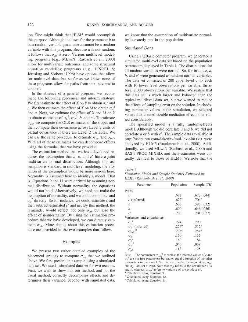
Table 1Simulation Model and Sample Statistics Estimated byHLM5 (Raudenbush et al., 2000)

Parameter Population Sample (SE)

Pathsc .672 .673 (.044)c (inferred) .672a .704a

a .600 .585 (.032)b .600 .646 (.036)c� .200 .201 (.027)

Variances and covariances�c

2 .274 .290�c

2 (inferred) .274b .312b

�(ab)2 .235c .254c

�a2 .160 .135

�b2 .160 .184

�c�2 .040 .058

�ab .113 .125

Note. The parameters �(ab)2 as well as the inferred values of c and

�c2 are not free parameters but rather equal a function of the other

parameters in the model. See the text for the formulas. Also, �ac�

and �bc� are set to zero. Note that �ab refers to the covariance of aand b, whereas �(ab)

2 refers to variance of the product ab.a Calculated using Equation 9.b Calculated using Equation 12.c Calculated using Equation 11.


method that we propose can use virtually any multi-level estimation computer program. Table 1 presentsthe population values of the parameters.

A random-effects mediational model was estimatedusing the Baron and Kenny (1986) steps. The result-ing parameter estimates from the simulation data setare displayed in the right column of Table 1. We nowuse HLM5 notation, not the notation that we haveused so far in the article, to describe the estimationsteps. First, using HLM5, we estimated the unmedi-ated effect of X on Y or path c. In this model the Level1 equation is Y � �0 + �1(X ) + r. The Level 2equations are �0 � �00 + u0 and �1 � �10 + u1.

Second, the effect of X on the mediator M, which ispath a in Figure 1, was estimated. The Level 1 equa-tion in this model using HLM5 notation is M � �0 +�1(X ) + r. The Level 2 equations for this model arethe same as those for the model of the unmediatedeffect, that is, �0 � �00 + u0 and �1 � �10 + u1.While estimating the effect of X on M, we created afile containing the OLS estimates of the Level 1 patha coefficients2 (i.e., the a coefficients for each indi-vidual), which are necessary to estimate �ab.

Next, the effects of M and X on Y—paths b and c�displayed in Figure 1, respectively—were estimated.In this model the Level 1 equation is Y � �0 + �1(X )+ �2(M ) + r, and the Level 2 equations are �0 � �00

+ u0, �1 � �10 + u1, and �2 � �20 + u2. As was donewith path a coefficients, a file containing the path bcoefficients was created.

Finally, the OLS estimates of the b coefficients andOLS estimates of the a coefficients (contained in thefirst residual file created) were then copied into asingle file and the covariance between a and b or �ab

was estimated. Lower level path a and path b coeffi-cients were correlated, r � .472, p < .01, with acovariance of .125, as displayed in Table 1. The dis-attenuated correlation between a and b (as opposed tothe correlation between estimated a and b) is .793.Table 1 displays a summary of population or theoret-ical and sample or estimated model parameters. Weused HLM5 to estimate the model parameters.

We can perform the decomposition of the total ef-fect both for the theoretical and empirical values. Thepopulation total effect or c is equal to .672. In thestandard single level model formulation (see Equation8), the total effect should equal the direct plus theindirect effect or 0.20 + (0.60)(0.60) or 0.56. Clearly,the standard single-level model formulation underes-timates the total effect. The population total effect0.672 is underestimated by 0.113, which exactly

equals the covariance between a and b. The popula-tion total effect inferred using the suggested formulafor random-effects models (Equation 9), which con-siders �ab, estimates the population total effect ex-actly. The population Level 2 variance of estimatedab using the suggested formula for random-effectsmodels (Equation 11) equals 0.235. This populationvariance is underestimated at 0.141 when the standardsingle level model approach, Equation 10, is used.

In the sample, the estimated total effect c, 0.673, isvirtually identical to the population value of 0.672.We can also decompose the sample total effect usingthe standard single level model approach to decom-position or Equation 8. This approach underestimatesthe total effect as 0.579. The correct equation for ran-dom-effects models, Equation 9, is closer to the totaleffect, somewhat overestimating it as 0.704. Using thesuggested formula for multilevel random-effects mod-els (Equation 11), we estimate �(ab)

2 as 0.254, whichis not that far from the population value, .234, andmuch closer than using the standard single levelmodel approach (Equation 10), which results in avalue of 0.144.

Finally, we examined how the introduction of themediator affects the variation in the effect of X on Y.In the population, �c

2 is 0.274 and �c�2 is 0.040. Thus,

the mediator explains 85% of the variation of theeffect of X on Y. Using sample estimates, �c

2 is esti-mated as 0.29 and �c�

2 as 0.058; therefore, the me-diator explains 80% of the variation of the effect of Xon Y.

Example Using an Existing Data Set

We next apply our estimation method for random-effects models to an actual data set. Korchmaros andKenny (2001) examined the mediation of genetic re-latedness on willingness to help by emotional close-ness. That is, the decision to help kin is mediated byfeelings of closeness. Korchmaros and Kenny (2002)followed up this study with an investigation of themediation of the effect of genetic relatedness on emo-tional closeness. It seemed very plausible that per-ceived similarity was a possible mediator. Korch-maros and Kenny (2002) asked persons to list their

2 Actually the residual file created by HLM5 (Rauden-bush et al., 2000) contains residual coefficients, the coeffi-cients minus the “average” coefficient. Because we seek tocompute a covariance between two sets of coefficients andcovariances subtract off the mean, this is not a problem.


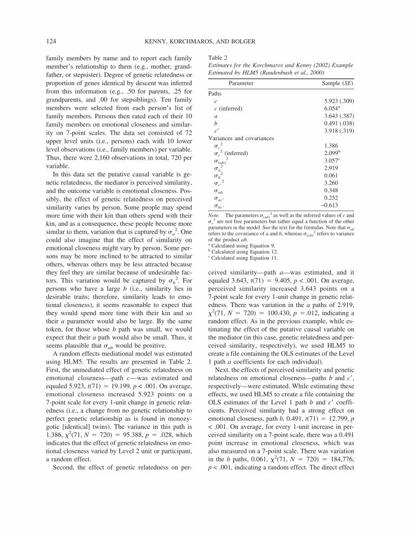
family members by name and to report each familymember’s relationship to them (e.g., mother, grand-father, or stepsister). Degree of genetic relatedness orproportion of genes identical by descent was inferredfrom this information (e.g., .50 for parents, .25 forgrandparents, and .00 for stepsiblings). Ten familymembers were selected from each person’s list offamily members. Persons then rated each of their 10family members on emotional closeness and similar-ity on 7-point scales. The data set consisted of 72upper level units (i.e., persons) each with 10 lowerlevel observations (i.e., family members) per variable.Thus, there were 2,160 observations in total, 720 pervariable.

In this data set the putative causal variable is ge-netic relatedness, the mediator is perceived similarity,and the outcome variable is emotional closeness. Pos-sibly, the effect of genetic relatedness on perceivedsimilarity varies by person. Some people may spendmore time with their kin than others spend with theirkin, and as a consequence, these people become moresimilar to them, variation that is captured by �a

2. Onecould also imagine that the effect of similarity onemotional closeness might vary by person. Some per-sons may be more inclined to be attracted to similarothers, whereas others may be less attracted becausethey feel they are similar because of undesirable fac-tors. This variation would be captured by �b

2. Forpersons who have a large b (i.e., similarity lies indesirable traits; therefore, similarity leads to emo-tional closeness), it seems reasonable to expect thatthey would spend more time with their kin and sotheir a parameter would also be large. By the sametoken, for those whose b path was small, we wouldexpect that their a path would also be small. Thus, itseems plausible that �ab would be positive.

A random effects mediational model was estimatedusing HLM5. The results are presented in Table 2.First, the unmediated effect of genetic relatedness onemotional closeness—path c—was estimated andequaled 5.923, t(71) � 19.199, p < .001. On average,emotional closeness increased 5.923 points on a7-point scale for every 1-unit change in genetic relat-edness (i.e., a change from no genetic relationship toperfect genetic relationship as is found in monozy-gotic [identical] twins). The variance in this path is1.386, �2(71, N � 720) � 95.388, p � .028, whichindicates that the effect of genetic relatedness on emo-tional closeness varied by Level 2 unit or participant,a random effect.

Second, the effect of genetic relatedness on per-

ceived similarity—path a—was estimated, and itequaled 3.643, t(71) � 9.405, p < .001. On average,perceived similarity increased 3.643 points on a7-point scale for every 1-unit change in genetic relat-edness. There was variation in the a paths of 2.919,�2(71, N � 720) � 100.430, p �.012, indicating arandom effect. As in the previous example, while es-timating the effect of the putative causal variable onthe mediator (in this case, genetic relatedness and per-ceived similarity, respectively), we used HLM5 tocreate a file containing the OLS estimates of the Level1 path a coefficients for each individual).

Next, the effects of perceived similarity and geneticrelatedness on emotional closeness—paths b and c�,respectively—were estimated. While estimating theseeffects, we used HLM5 to create a file containing theOLS estimates of the Level 1 path b and c� coeffi-cients. Perceived similarity had a strong effect onemotional closeness, path b, 0.491, t(71) � 12.799, p< .001. On average, for every 1-unit increase in per-ceived similarity on a 7-point scale, there was a 0.491point increase in emotional closeness, which wasalso measured on a 7-point scale. There was variationin the b paths, 0.061, �2(71, N � 720) � 184,776,p < .001, indicating a random effect. The direct effect

Table 2Estimates for the Korchmaros and Kenny (2002) ExampleEstimated by HLM5 (Raudenbush et al., 2000)

Parameter Sample (SE)

Pathsc 5.923 (.309)c (inferred) 6.054a

a 3.643 (.387)b 0.491 (.038)c� 3.918 (.319)

Variances and covariances�c

2 1.386�c

2 (inferred) 2.099b

�(ab)2 3.057c

�a2 2.919

�b2 0.061

�c�2 3.260

�ab 0.348�ac� 0.252�bc� −0.613

Note. The parameters �(ab)2 as well as the inferred values of c and

�c2 are not free parameters but rather equal a function of the other

parameters in the model. See the text for the formulas. Note that �ab

refers to the covariance of a and b, whereas �(ab)2 refers to variance

of the product ab.a Calculated using Equation 9.b Calculated using Equation 12.c Calculated using Equation 11.


of genetic relatedness on emotional closeness was re-duced, though remained strong being equal to 3.918,t(71) � 12.272, p < .001.

The lower level path aj and path bj coefficientswere correlated, r � .262, p � .026, with a covari-ance of 0.348 and a disattenuated correlation of .825.Also using the OLS paths, we estimated3 �ac� as 0.252and �bc� as −0.613, only the latter covariance beingstatistically significant.

Consider the decomposition of the effects of themediational model. Using the standard single levelmodel formula where the �ab is not considered, thetotal effect is 5.706, 3.918 + (3.643)(0.491), whichunderestimates c, the actual unmediated path coeffi-cient (5.923) by 0.217. By this computation of thetotal effect, only 31% of the total effect, (5.706 −3.918)/5.706, is mediated. When using the suggestedrandom-effects formula where the �ab is considered,the total effect is 6.054, 3.918 + (3.643)(0.491) +0.348, which somewhat overestimates the unmediatedpath coefficient by 0.131. By this computation of thetotal effect, 35% of the total effect, (6.054 − 3.918)/6.054, is mediated. These proportions of the total ef-fect illustrate the importance of considering �ab whenestimating the amount of mediation. However, notethat these proportions may not characterize the popu-lation because they are calculated using sample esti-mates from a relatively small sample. The importanceof considering �ab when estimating the amount ofmediation is also illustrated in the variance of themediated effects or �(ab)

2. This variance or �(ab)2

equals 1.691 for the standard single-level modelspecification (Equation 10) and 3.057 when allow-ances for �ab are made (Equation 11).

Very surprisingly, introducing the mediator in-creases the variance in the effect of X on Y. Withouthaving the mediator in the model, the variance of c is1.386, but having the mediator in the equation leads toa variance of c� of 3.260. We suspect that the follow-ing might be happening. There is relatively littlevariation in the total effect of genetic relatedness andemotional closeness—for most people there is astrong relationship between genetic relatedness andemotional closeness. However, people may vary interms of the reason why this relationship exists. Forsome people, the relationship between genetic relat-edness and emotional closeness is completely medi-ated by similarity, whereas for others, other variablessuch as frequency of interaction might partially me-diate the relationship. The negative correlation be-tween b and c� is consistent with this explanation.

When there is more mediation, leading to larger bpaths, the c� path is smaller; and when there is lessmediation, leading to smaller b paths, the c� path islarger. Additionally, the inferred variance of c issomewhat overestimated. This is possibly because ofnonnormality (or see Footnote 3).

Conclusion

Multilevel models are being increasingly used toestimate models for both repeated measures andnested data. We consider the use of multilevel mod-eling to estimate mediational models in which there islower level mediation, and all terms are random. Weshow that the standard formulas for indirect effectsand their variance must be modified for this type ofmodel. For each, the covariance between path a and bshould be considered.

None of the standard methods of estimating multi-level models can estimate such a model. We suggestan ad hoc procedure that uses conventional methods.We present an example using simulated data, and wesee that our method adequately captures the model’sparameters. We also present an example using an ex-isting data set. These examples illustrate that ourmethod provides quite different and more accurateresults than using conventional methods that havebeen used in single level models.

This method, though adequate, is less than ideal.First, it does not exactly reproduce the total effect asis estimated by the unmediated model. There are afew reasons for this inexact estimation. One reason isthat maximum-likelihood estimation weights the esti-mates differently when the mediator is in the modeland when it is not. Some of the difference between thecoefficient of the X-to-Y path in the mediated modeland the corresponding coefficient in the unmediatedmodel is due to this difference in weighting ratherthan to mediation (Krull & MacKinnon, 1999). Notethat a similar problem can arise for standard, singlelevel mediational models when X, M, or Y are definedas latent variables or when logistic regressions arerun. Because of maximum-likelihood estimation, theoverall X-to-Y effect can change when the mediator Mis included in the model.

3 Because b and c� are estimated from the same equation,they contain correlated sampling error that is ignored in theOLS estimation method of the covariance. The presence ofthis correlated sampling error likely biases the estimate of�bc�.


A second limitation of the proposed procedure isthat we use OLS estimation to calculate �ab and donot weight a and b by their statistical precision. Anideal estimator of the covariance would take the sta-tistical precision of a and b into account. Additionally,although we do provide for a statistical test for �ab

using the correlation of the estimates of a and b, wedo not directly estimate its standard error.

Finally, the estimation method that we have devel-oped requires the assumption that a, b, and c� have ajoint multivariate normal distribution. Although thisassumption is standard in multilevel modeling, asmentioned previously, the violation of the assumptionmight be more serious here. This is because normalityis assumed to identify a model.

We view our method as only an interim method,and we expect that a single step estimation methodwill be developed to replace our piecemeal approach.Ideally, a computer program would simultaneouslyestimate several multilevel models (one for M and onefor Y ) and allow for paths between outcome variables(from M to Y ). With these programs, it would bepossible to simultaneously estimate the Level 1 a andb coefficients and also to estimate �ab. It would beeven better if the program would have an option fornonnormal distributions of a and b. Given that struc-tural equation modeling software is beginning to in-clude multilevel capabilities (e.g., LISREL 8[Joreskog & Sorbom, 1996]; EQS [Bentler, 1995];Mplus [Muthen & Muthen, 2002]; Mx [Neale, 2002]),and multilevel software is beginning to add structuralequation modeling capabilities (HLM5), we expectthat single-step estimation methods will soon be avail-able.

There are additional limits in our approach. First,we make all of the usual assumptions of multilevelmodeling. One standard assumption of that approachis that the random effects have a multivariate normaldistribution. Some of the formulas are based on theassumption of multivariate normality. However, weneed not make that assumption because we can com-pute c and �c

2 directly. We have assumed that a andb have a bivariate normal distribution. Equations 9,11, and 12 would be much more complex if we allowthe distributions of a and b to be nonnormal. Becauseit is already standard practice to assume normal dis-tributions and because the formulas are already verycomplicated, we do not consider nonnormality in thisarticle. A recent article by Shrout and Bolger (2002)used bootstrapping to estimate and to take account ofnonnormality in the sampling distribution of ab in a

fixed-effects mediational model. Although it wouldbe considerably more difficult to implement, it is pos-sible that this or some similar approach may be usefulin tackling nonnormality in the random-effects case.

Second, we assume that the mediational model iscorrectly specified. A mediational model is a causalmodel. Ideally the variable X is a manipulated vari-able, and consequently, we know that if there is astatistical association, then X causes M and Y, and notvice versa. The variable M is not manipulated and sothe assumption that M causes Y is more problematic.Both substantive theory and research design (e.g.,measuring M before Y) should be used to justify thecausal direction. One key assumption is that there isno measurement error in either M or X. If there weremeasurement error in either of these variables, differ-ent methods would have to be used (Raudenbush &Sampson, 1999).

A statistical mediational analysis never establishesor proves mediation. Mediation occurs when a puta-tive causal variable causes the putative mediator,which causes an outcome. Causation is a logical, theo-retical, and experimental issue. A statistical analysisby itself cannot prove causation and, consequently,cannot prove mediation. For instance, seemingly cred-ible estimates can often be obtained if Y is treated asthe mediator and M is treated as the outcome. Likeother causal models, a mediational analysis can estab-lish that the model is false; however, it cannot everprove that it is true.

We do believe that studying mediation with a mul-tilevel context affords a much greater understandingof the process than a single level analysis. First andforemost, we can test to see if the mediation is thesame for all upper level units. If there is no variation,then we gain confidence that the process is universal.Second, if we find that the mediation varies by upperlevel unit, then we can see if that variation is mean-ingful theoretically. So, for instance, if some people(or groups in the case where groups are the Level 2unit) show the mediation and others do not, then wecan investigate why we get mediation for some peopleand not for others. In this way we can probe theoriesin greater detail. However, some methodologistsmight question interpreting mediation as a causal ef-fect when that mediational effect varies randomly.

Third, we have considered only lower level media-tion. However, upper level mediation is considered inother articles (Krull & MacKinnon, 1999; Rauden-bush & Sampson, 1999).

Multilevel models are now becoming common in


the social and behavioral sciences. These models al-low researchers to study important social processessuch as how intimate relationships affect the course ofa person’s health and psychological well-being (e.g.,Bolger, Zuckerman, & Kessler, 2000) and how social-structural variables affect the likelihood of individuallevel victimization (Sampson, Raudenbush, & Earls,1997). We hope that by providing a method of assess-ing mediation in multilevel models, their value to re-searchers will be substantially increased.

References

Aroian, L. A. (1947). The probability function of the prod-uct of two normally distributed variables. The Annals ofMathematical Statistics, 18, 265–271.

Baron, R. M., & Kenny, D. A. (1986). The moderator–mediator variable distinction in social psychological re-search: Conceptual, strategic, and statistical consider-ations. Journal of Personality and Social Psychology, 51,1173–1182.

Bentler, P. M. (1995). EQS structural equations programmanual [Computer software manual]. Encino, CA: Mul-tivariate Software.

Bolger, N., Davis, A., & Rafaeli, E. (2003). Diary methods:Capturing life as it is lived. Annual Review of Psychol-ogy, 54, 579–616.

Bolger, N., & Zuckerman, A. (1995). A framework forstudying personality in the stress process. Journal of Per-sonality and Social Psychology, 69, 890–902.

Bolger, N., Zuckerman, A., & Kessler, R. C. (2000). Invis-ible support and adjustment to stress. Journal of Person-ality and Social Psychology, 79, 953–961.

Diggle, P., Heagerty, P., Liang, K. Y., & Zeger, S. (2001).Analysis of longitudinal data. New York: Oxford Univer-sity Press.

Goodman, L. A. (1960). On the exact variance of products.Journal of the American Statistical Association, 55, 708–713.

Hox J. (2002). Multilevel analyses: Techniques and appli-cations. Mahwah, NJ: Erlbaum.

Joreskog, K. G., & Sorbom, D. (1996). LISREL 8 user’sreference guide [Computer software manual]. Chicago:Scientific Software International.

Judd, C. M., Kenny, D. A., & McClelland, G. H. (2001).Estimating and testing mediation and moderation inwithin-subjects designs. Psychological Methods, 6, 115–134.

Kendall, M. G., & Stuart, A. (1958). The advanced theory ofstatistics (Vol. 1). London: Griffin.

Kenny, D. A., Kashy, D. A., & Bolger, N. (1998). Dataanalysis in social psychology. In D. Gilbert, S. T. Fiske,& G. Lindzey (Eds.), The handbook of social psychology(4th ed., Vol. 1, pp. 223–265). New York: McGraw-Hill.

Korchmaros, J. D., & Kenny, D. A. (2001). Emotionalcloseness as a mediator of the effect of genetic related-ness on altruism. Psychological Science, 12, 262–265.

Korchmaros, J. D., & Kenny, D. A. (2002). An evolutionaryand close relationship model of helping. Manuscript sub-mitted for publication.

Kreft, I. G. G., DeLeeuw, J., & Aiken, L. S. (1995). Vari-able centering in hierarchical linear models: Model pa-rameterization, estimation, and interpretation. Multivari-ate Behavioral Research, 30, 1–21.

Krull, J. L., & MacKinnon, D. P. (1999). Multilevel media-tion modeling in group-based intervention studies. Evalu-ation Review, 23, 418–444.

Krull, J. L., & MacKinnon, D. P. (2001). Multilevel mod-eling of individual and group level mediated effects. Mul-tivariate Behavioral Research, 36, 249–277.

MacKinnon, D. P., Warsi, G., & Dwyer, J. H. (1995). Asimulation study of mediated effect measures. Multivari-ate Behavioral Research, 30, 41–62.

Muthen, B. O., & Muthen, L. K. (2002). Mplus version 2user’s guide [Computer software manual]. Los Angeles:Muthen & Muthen.

Neale, M. C. (2002). Mx: Statistical modeling [Computersoftware manual]. Richmond: Virginia CommonwealthUniversity.

Rasbash, J., Browne, W., Goldstein, H., Yang, M., Plewis,I., Healy, M., et al. (2000). A user’s guide to MlwiN(Version 2.1) [Computer software manual]. London: Uni-versity of London, Institute of Education, MultilevelModels Project.

Raudenbush, S. W., & Bryk, A. S. (1986). A hierarchicalmodel for studying school effects. Sociology of Educa-tion, 59, 1–17.

Raudenbush, S. W., & Bryk, A. S. (2002). Hierarchical lin-ear models: Applications and data analysis methods (2nded.). Thousand Oaks, CA: Sage.

Raudenbush, S. W., Bryk, A. S., Cheong, Y. F., & Cong-don, R. (2000). HLM5: Hierarchical linear and nonlin-ear modeling [Computer software manual]. Lincoln-wood, IL: Scientific Software International.

Raudenbush, S. W., & Sampson, R. (1999). Assessing di-rect and indirect effects in multilevel designs with latentvariables. Sociological Methods and Research, 28, 123–153.


Sampson, R. J., Raudenbush, S. W., & Earls, F. (1997, Au-gust 15). Neighborhoods and violent crime: A multilevelstudy of collective efficacy. Science, 277, 918–924.

Shrout, P. E., & Bolger, N. (2002). Mediation in experimen-tal and nonexperimental studies: New procedures andrecommendations. Psychological Methods, 7, 422–445.

Snijders, T. A., & Bosker, R. J. (1999). Multilevel analysis:An introduction to basic and advanced multilevel model-ing. Thousand Oaks, CA: Sage.

Sobel, M. E. (1982). Asymptotic confidence intervals forindirect effects in structural models. In S. Leinhardt (Ed.),Sociological methodology 1982 (pp. 290–312). San Fran-cisco: Jossey-Bass.

Received January 4, 2002Revision received February 10, 2003

Accepted February 10, 2003 �


Documents

Lower Level Mediation in Multilevel Modelsnb2229/docs/kenny-korchmaros-bolger-pm-2003.… · Lower Level Mediation in Multilevel Models David A. Kenny and ... tional states (e.g.,