Embed Size (px)
Citation preview
Structural Equation Modeling, 18:161–182, 2011
Copyright © Taylor & Francis Group, LLC
ISSN: 1070-5511 print/1532-8007 online
DOI: 10.1080/10705511.2011.557329
Alternative Methods for AssessingMediation in Multilevel Data:
The Advantages of Multilevel SEM
Kristopher J. PreacherDepartment of Psychology, University of Kansas
Zhen ZhangDepartment of Management, Arizona State University
Michael J. ZyphurDepartment of Management and Marketing, University of Melbourne
Multilevel modeling (MLM) is a popular way of assessing mediation effects with clustered data.
Two important limitations of this approach have been identified in prior research and a theoretical
rationale has been provided for why multilevel structural equation modeling (MSEM) should
be preferred. However, to date, no empirical evidence of MSEM’s advantages relative to MLM
approaches for multilevel mediation analysis has been provided. Nor has it been demonstrated that
MSEM performs adequately for mediation analysis in an absolute sense. This study addresses these
gaps and finds that the MSEM method outperforms 2 MLM-based techniques in 2-level models in
terms of bias and confidence interval coverage while displaying adequate efficiency, convergence
rates, and power under a variety of conditions. Simulation results support prior theoretical work
regarding the advantages of MSEM over MLM for mediation in clustered data.
Keywords: mediation, multilevel modeling, multilevel SEM, structural equation modeling
Most methods for addressing mediation hypotheses were designed for data collected using
simple random sampling. However, researchers are increasingly collecting data organized in
two or more hierarchical levels, such as children nested within schools, or repeated measures
nested within individuals. Traditional multiple linear regression (MLR) methods for assessing
Correspondence should be addressed to Kristopher J. Preacher, Department of Psychology, University of Kansas,
1415 Jayhawk Blvd., Rm. 426, Lawrence, KS 66045-7556, USA. E-mail: [email protected]
161
Downloaded By: [University of Kansas] At: 20:23 14 April 2011
162 PREACHER, ZHANG, ZYPHUR
mediation (e.g., Baron & Kenny, 1986; MacKinnon, Lockwood, Hoffman, West, & Sheets,
2002; MacKinnon, Warsi, & Dwyer, 1995) are inappropriate in multilevel settings, primarily
because the assumption of independence of observations is violated in clustered data. Con-
sequently, there is a growing awareness that clustering needs to be taken into account when
statistically assessing mediation effects.
Multilevel modeling (MLM)—sometimes referred to as hierarchical linear modeling, random
coefficient modeling, or mixed-effects modeling—is a family of regression-based methods
that can be greatly superior to multiple linear regression when data are clustered in some
fashion (Kreft & de Leeuw, 1998; Raudenbush & Bryk, 2002; Snijders & Bosker, 1999).
MLM incorporates different error terms for different levels of the data hierarchy, yields more
accurate Type I error rates than nonhierarchical methods, and permits intercepts and slopes to
vary randomly across clusters. But exactly how to use MLM to address mediation hypotheses
with clustered data has proven controversial. Several papers published over the last decade
present MLM strategies for assessing multilevel mediation (Bauer, Preacher, & Gil, 2006;
Kenny, Korchmaros, & Bolger, 2003; Krull & MacKinnon, 1999, 2001; MacKinnon, 2008;
Pituch & Stapleton, 2008; Pituch, Stapleton, & Kang, 2006; Pituch, Murphy, & Tate, 2010;
Pituch, Whittaker, & Stapleton, 2005; Raudenbush & Sampson, 1999; Z. Zhang, Zyphur, &
Preacher, 2009). More recently, Preacher, Zyphur, and Zhang (2010) identified two major
limitations associated with the MLM family of techniques when applied to mediation analysis.
First, although MLM methods have proven useful for designs in which the independent variable
X is assessed at either level and the mediator M and outcome variable Y are assessed at
Level 1, MLM cannot accommodate upper level mediators or outcome variables. Therefore,
theoretical models involving Level 2 variables being predicted by Level 1 or Level 2 variables
in these roles (e.g., models for so-called 1–1–2 or 1–2–2 designs,1 using a notation convention
suggested by Krull & MacKinnon, 2001) cannot be fit using MLM. Second, for multilevel
mediation models involving linkages between pairs of Level 1 variables (e.g., the M ! Y
effect in a 2–1–1 design), the Within and Between components of these effects are conflated
in many traditional applications of MLM. That is, the effect of M on Y within clusters and
the effect of M on Y between clusters are implicitly constrained to be equal. In the context of
this study we term the application of MLM that conflates Within and Between components of
effects conflated multilevel modeling (CMM).
A common device used to separate Level 1 effects into Within and Between components
is to group mean center the Level 1 predictor and introduce the cluster mean as a Level 2
predictor (Hedeker & Gibbons, 2006; Kreft & de Leeuw, 1998; Raudenbush & Bryk, 2002;
Shin & Raudenbush, 2010; Snijders & Bosker, 1999). In the context of mediation analysis,
Krull and MacKinnon (2001), MacKinnon (2008), and Z. Zhang et al. (2009) suggested
“unconflating” Level 1 effects in mediation models that include 1–1 linkages, a strategy we
term unconflated multilevel modeling (UMM). However, even though the resulting Between
effect is separated from the Within effect, the Between effect is biased toward the Within
effect to the extent that intraclass correlations2 (ICCs) are low and cluster sizes are small.
This bias, in turn, will also contribute to bias in any Between-level indirect effect of which it
1For example, 1–2–2 denotes a design in which the independent variable X is assessed at Leve1 1, whereas both
the mediator M and outcome Y are assessed at Level 2.2ICC is often interpreted as the proportion of variability in a variable that is between-cluster.
Downloaded By: [University of Kansas] At: 20:23 14 April 2011
MULTILEVEL SEM FOR MEDIATION 163
serves as a component effect. To overcome these limitations, Preacher et al. (2010) suggested
that multilevel structural equation modeling (MSEM) should be used to investigate mediation
effects in clustered data.
Prior research has shown that the traditional MLM approach has multiple differences from
what we refer to as MSEM. First, in MLM, group means are used at Level 2 to represent group
standings on a Level 1 predictor variable (Raudenbush & Bryk, 2002), which, as noted earlier,
biases Between effects. In MSEM, group standings on all Level 1 variables are treated as latent,
thereby correcting for sampling error. Second, in traditional MLM, variables are observed and
measurement error is not accounted for in model estimation, whereas MSEM allows for the
inclusion of traditional latent variables to account for measurement error (Marsh et al., 2009).
Third, traditional MLM conflates Between- and Within-level effects of Level 1 variables on
other Level 1 variables (MacKinnon, 2008; Z. Zhang et al., 2009). In MSEM, the Between and
Within parts of all variables are separated, allowing for an examination of direct and indirect
effects at each level, as well as contextual effects across levels. With these features of the
MSEM approach, Preacher et al. (2010) proposed it as a useful tool for researchers interested
in investigating multilevel mediation.
Despite Preacher et al.’s (2010) theoretical developments, there remains no empirical evi-
dence that the MSEM method for multilevel mediation accomplishes what it is intended to.
Lüdtke et al. (2008) showed that MSEM dramatically reduces bias in contextual effects relative
to a group mean-centered MLM approach. However, their study did not examine indirect effects
or the conflation of Within and Between components of effects, nor did they address the ability
of MSEM to include upper level outcomes. Hence, it is unclear to what extent the findings of
Lüdtke et al. generalize to the estimation of indirect effects. That is, no research has shown
that MSEM reduces or eliminates bias in indirect effects to a substantially greater degree than
traditional conflated and unconflated MLM approaches. It also has not been demonstrated that
MSEM performs well at estimating and testing indirect effects in an absolute sense. That is,
apart from our expectation that MSEM is superior to MLM-based methods in terms of bias, it is
hoped that MSEM performs adequately in terms of confidence interval (CI) coverage, efficiency
of estimation, model convergence, and statistical power for detecting nonzero indirect effects.
Addressing these unanswered questions is the purpose of this study.
In this study, we address two goals via simulation. Regarding the first goal, based on
developments and findings reported by Preacher et al. (2010) and Lüdtke et al. (2008), we
hypothesize that MSEM will demonstrate dramatically reduced bias in Between indirect effects
relative to competing MLM-based approaches. Regarding the second goal, based on prior
MSEM simulations outside the mediation context, we hypothesize that MSEM will demonstrate
adequate performance in terms of achieving nominal CI coverage and show low absolute levels
of estimation variability (i.e., high efficiency), adequate model convergence rates, and adequate
power for detecting nonzero indirect effects. In our simulation, bias is considered acceptably
small if it lay (arbitrarily) between ˙5% of 0, nominal coverage is 95%, adequate convergence
rates are set arbitrarily at 95%, and adequate power is taken to be at least .80 (Cohen, 1988).
It is not possible to set meaningful benchmarks for low estimation variability, except to note
that smaller is better, all else being equal. We are also interested in the performance of MSEM
at low ICCs, as Lüdtke et al. (2008) encountered more estimation problems at smaller ICCs.
These hypotheses are treated in more detail in a later section with respect to the specific model
chosen for simulation.
Downloaded By: [University of Kansas] At: 20:23 14 April 2011
164 PREACHER, ZHANG, ZYPHUR
METHODS TO BE COMPARED
The three methods we describe are compared using data simulated from a 2–1–1 design that
is common in the applied literature (e.g., Hom et al., 2009; Komro et al., 2001; Piontek et al.,
2008; Roth, Assor, Kanat-Maymon, & Kaplan, 2007). Because the independent variable (Xj )
in the 2–1–1 design varies strictly between clusters, the indirect effect in such a design must be
a Between indirect effect; that is, any effect of Xj , indirect or otherwise, must be a Between
effect because Xj cannot covary with within-cluster individual differences. The 2–1–1 design
also includes a 1–1 link between Mij and Yij , allowing us to investigate the performance of
the various methods when the Between and Within components of this effect differ in the
population.
Conflated Multilevel Modeling
The first method we consider is traditional MLM with conflated Within and Between effects.
A variety of pure MLM and hybrid MLR/MLM models have been proposed for assessing
mediation (Krull & MacKinnon, 1999, 2001; Pituch & Stapleton, 2008; Pituch, Stapleton,
& Kang, 2006; Raudenbush & Sampson, 1999). Kenny et al. (2003) and Bauer et al.
(2006) described a multilevel model for 1–1–1 designs that permits random intercepts and
fixed or random slopes for all 1-1 links. Because we use a 2–1–1 design for purposes
of the simulation, we adopt the random-intercept, fixed-slope model for 2–1–1 designs
described by Krull and MacKinnon (1999, 2001), MacKinnon (2008), and Pituch and Stapleton
(2008):
Mij D “M0j C eMij
“M0j D ”M00 C ”M01Xj C uM0j
(1)
Yij D “Y 0j C “Y 1j Mij C eY ij
“Y 0j D ”Y 00 C ”Y 01Xj C uY 0j
“Y 1j D ”Y 10
(2)
where i indexes Level 1 units; j indexes Level 2 units; “M0j and “Y 0j are random intercepts;
”M00 and ”Y 00 are fixed intercept means; ”M01, ”Y 01, and ”Y 10 are fixed slopes; eMij and eY ij
are Level 1 residuals; and uM0j and uY 0j are Level 2 residuals. The indirect effect in this model
is a Between indirect effect, quantified as ”M01 � ”Y 10, because Xj is a purely cluster-level
variable. In estimating only one effect of Mij on Yij without first separating Mij into Within
and Between components, this MLM approach conflates the Within and Between components
of this effect. That is, ”Y 10 is a weighted average of the effects of the Between and Within
components of Mij on Yij (Preacher et al., 2010; Z. Zhang et al., 2009), and assumes that the
contextual effect is zero. Thus, the Between indirect effect is likely to be biased if the Within
and Between effects actually differ.
Downloaded By: [University of Kansas] At: 20:23 14 April 2011
MULTILEVEL SEM FOR MEDIATION 165
Unconflated Multilevel Model
To address the conflation problem, Krull and MacKinnon (2001), MacKinnon (2008), and
Z. Zhang et al. (2009) proposed explicitly separating Within and Between components of
variables in mediation models into between-cluster components (cluster means) and within-
cluster components (deviations from cluster means). Z. Zhang et al. (2009) concentrated on
2–1–1 designs, with the expectation that results would also apply to 1–1–1 designs. The model
equations are:
Mij D “M0j C eMij
“M0j D ”M00 C ”M01Xj C uM0j
(3)
Yij D “Y 0j C “Y 1j .Mij � M:j / C eY ij
“Y 0j D ”Y 00 C ”Y 01Xj C ”Y 02M:j C uY 0j ;
“Y 1j D ”Y 10
(4)
where M:j is the cluster mean of Mij and other terms are as previously defined. Because Xj
is a purely Between cluster construct, the only indirect effect that can occur in this model is
a Between indirect effect. Thus, the indirect effect is quantified as ”M01 � ”Y 02. Note that this
model reduces to the CMM for 2–1–1 data when ”Y 02 (the Between effect of Mij on Yij ) and
”Y 10 (the Within effect of Mij on Yij ) are constrained to equality.
Despite the fact that this procedure explicitly addresses the conflation issue, problems remain.
First, because the method is presented within the MLM framework, it still suffers from the
limitation that outcome variables must be assessed at Level 1. Consequently, whereas the
UMM method accommodates 2–1–1 and 1–1–1 designs, it cannot accommodate other plausible
three-variable designs, including 2–2–1, 1–1–2, 1–2–2, 1–2–1, and 2–1–2 designs, all of which
involve at least one linkage in which a Level 2 variable serves as the dependent variable.
Second, even though the UMM method separates Within and Between effects, the Between
effects nevertheless are biased toward the corresponding Within effects (Preacher et al., 2010).
Multilevel Structural Equation Modeling
To address the limitations of the various MLM approaches for assessing mediation in nested
data, Preacher et al. (2010) proposed using an MSEM approach pioneered by B. O. Muthén
and Asparouhov (2008). The MSEM framework is general enough to accommodate binary,
ordered categorical, continuous normal, and count variables, latent categorical variables, and
finite mixtures. Here we focus on continuous normally distributed variables without latent
classes or mixtures. The two-level MSEM is represented in Equations 5 through 7:
Level 1 measurement model: Yij D �j C ƒj ˜ij C Kj Xij C ©ij (5)
Level 1 structural model: ˜ij D ’j C Bj ˜ij C �j Xij C —ij (6)
Level 2 structural model: ˜j D � C “˜j C ”Xj C —j (7)
Downloaded By: [University of Kansas] At: 20:23 14 April 2011
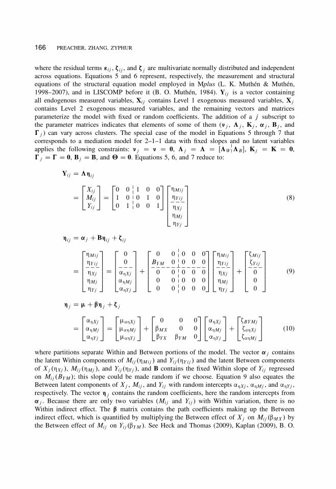
166 PREACHER, ZHANG, ZYPHUR
where the residual terms ©ij , —ij , and —j are multivariate normally distributed and independent
across equations. Equations 5 and 6 represent, respectively, the measurement and structural
equations of the structural equation model employed in Mplus (L. K. Muthén & Muthén,
1998–2007), and in LISCOMP before it (B. O. Muthén, 1984). Yij is a vector containing
all endogenous measured variables, Xij contains Level 1 exogenous measured variables, Xj
contains Level 2 exogenous measured variables, and the remaining vectors and matrices
parameterize the model with fixed or random coefficients. The addition of a j subscript to
the parameter matrices indicates that elements of some of them (�j , ƒj , Kj , ’j , Bj , and
�j ) can vary across clusters. The special case of the model in Equations 5 through 7 that
corresponds to a mediation model for 2–1–1 data with fixed slopes and no latent variables
applies the following constraints: �j D � D 0, ƒj D ƒ D ŒƒW ––
ƒB �, Kj D K D 0,
�j D � D 0, Bj D B, and ‚ D 0. Equations 5, 6, and 7 reduce to:
Yij D ƒ˜ij
D
2
4
Xij
Mij
Yij
3
5 D
2
4
0 0 1 0 0
1 0 0 1 0
0 1 0 0 1––
––
– 3
5
2
6
6
6
6
4
˜Mij
˜Y ij– – –˜Xj
˜Mj
˜Yj
3
7
7
7
7
5
(8)
˜ij D ’j C B˜ij C —ij
D
2
6
6
6
6
4
˜Mij
˜Y ij– – –˜Xj
˜Mj
˜Yj
3
7
7
7
7
5
D
2
6
6
6
6
4
0
0– – –’˜Xj
’˜Mj
’˜Yj
3
7
7
7
7
5
C
2
6
6
6
6
4
0 0 0 0 0
BYM 0 0 0 0– – – – – – – – – – –
0 0 0 0 0
0 0 0 0 0
0 0 0 0 0––
––
––
––
– 3
7
7
7
7
5
2
6
6
6
6
4
˜Mij
˜Y ij– – –˜Xj
˜Mj
˜Yj
3
7
7
7
7
5
C
2
6
6
6
6
4
—Mij
—Y ij– – –
0
0
0
3
7
7
7
7
5
(9)
˜j D � C “˜j C —j
D
2
4
’˜Xj
’˜Mj
’˜Yj
3
5 D
2
4
�’˜Xj
�’˜Mj
�’˜Yj
3
5 C
2
4
0 0 0
“MX 0 0
“YX “YM 0
3
5
2
4
’˜Xj
’˜Mj
’˜Yj
3
5 C
2
4
—BYMj
—’˜Xj
—’˜Mj
3
5 (10)
where partitions separate Within and Between portions of the model. The vector ’j contains
the latent Within components of Mij .˜Mij / and Yij .˜Y ij / and the latent Between components
of Xj .˜Xj /, Mij .˜Mj /, and Yij .˜Yj /, and B contains the fixed Within slope of Yij regressed
on Mij .BYM /; this slope could be made random if we choose. Equation 9 also equates the
Between latent components of Xj , Mij , and Yij with random intercepts ’˜Xj , ’˜Mj , and ’˜Yj ,
respectively. The vector ˜j contains the random coefficients, here the random intercepts from
’j . Because there are only two variables (Mij and Yij ) with Within variation, there is no
Within indirect effect. The “ matrix contains the path coefficients making up the Between
indirect effect, which is quantified by multiplying the Between effect of Xj on Mij .“MX / by
the Between effect of Mij on Yij .“YM /. See Heck and Thomas (2009), Kaplan (2009), B. O.
Downloaded By: [University of Kansas] At: 20:23 14 April 2011
MULTILEVEL SEM FOR MEDIATION 167
Muthén and Asparouhov (2008), and Preacher et al. (2010) for more thorough explanations of
the general MSEM and its capabilities.
SIMULATION
Simulation Design
The population data-generating model was a model for 2–1–1 data with fixed slopes, but
findings obtained are expected to generalize to other mediation models containing 1–1 rela-
tionships, with or without fixed slopes. The 2–1–1 model was chosen specifically because here
only the Between indirect effect exists, so interest lies in unbiased estimation of the product
of Between path coefficients—one of the areas of weakness for the CMM approach that was
highlighted earlier. In addition, the 2–1–1 model has been used extensively by researchers
testing substantive research questions (e.g., Hom et al., 2009; Komro et al., 2001; Piontek
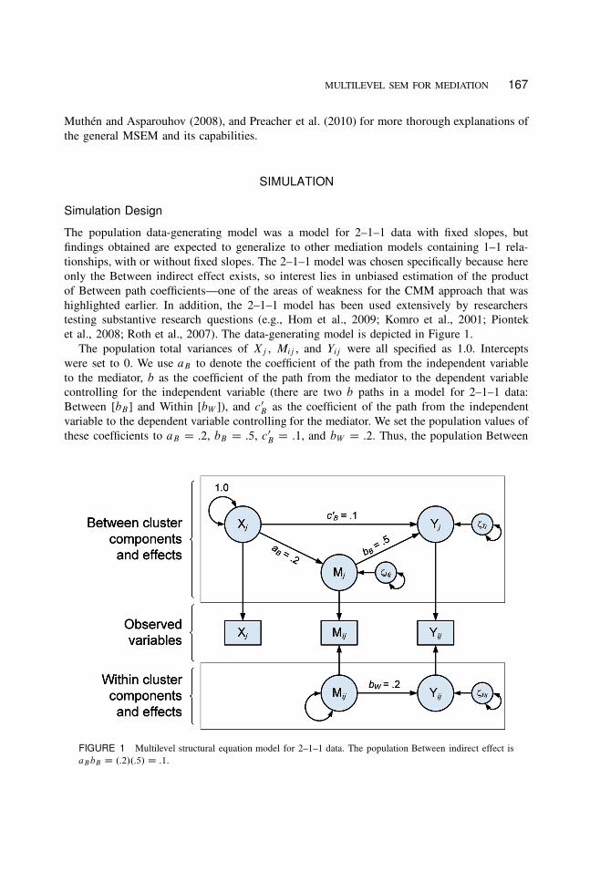
et al., 2008; Roth et al., 2007). The data-generating model is depicted in Figure 1.
The population total variances of Xj , Mij , and Yij were all specified as 1.0. Intercepts
were set to 0. We use aB to denote the coefficient of the path from the independent variable
to the mediator, b as the coefficient of the path from the mediator to the dependent variable
controlling for the independent variable (there are two b paths in a model for 2–1–1 data:
Between [bB ] and Within [bW ]), and c0
B as the coefficient of the path from the independent
variable to the dependent variable controlling for the mediator. We set the population values of
these coefficients to aB D :2, bB D :5, c0
B D :1, and bW D :2. Thus, the population Between
FIGURE 1 Multilevel structural equation model for 2–1–1 data. The population Between indirect effect is
aB bB D .:2/.:5/ D :1.
Downloaded By: [University of Kansas] At: 20:23 14 April 2011
168 PREACHER, ZHANG, ZYPHUR
indirect effect was aBbB D .:2/.:5/ D :1. Population ICCs for Mij and Yij were identical,
and were set to ICCM D ICCY D .05, .10, .20, or .40 to span values commonly encountered
in practice.3 Because the population Between regression weights were held constant across
all conditions, the Between R2 for the Mij equation was .8, .4, .2, and .1 for the four ICCs.
Similarly, the Between R2 for the Yij equation was .85, 55, .40, and .325. The number of
Level 2 units was specified as J D 20, 50, 100, 300, 500, or 1,000, and the number of
Level 1 units was nj D 5, 20, or 50.4 Each of these sample sizes was chosen to span values
encountered in typical multilevel research. Crossing conditions defined by ICC, J , and nj
resulted in 4 � 6 � 3 D 72 conditions. In each condition, 2,000 samples were generated using
a Fortran program for a total of 144,000 samples.
In our simulation, each of these 144,000 samples was fit with the CMM, UMM, and
MSEM models using Mplus version 5.21 (L. K. Muthén & Muthén, 1998–2007). One way
to gauge which of these strategies is to be preferred depends on the accuracy and efficiency
with which the relevant indirect effect is estimated, as well as the accuracy of CI coverage.
Additional practical concerns include the frequency with which the modeling method fails
due to convergence errors or estimation problems, and the degree to which a method yields
power high enough to detect an effect, if present. Next we outline our specific predictions
with regard to bias, coverage, efficiency, convergence, and power for these three alternative
modeling approaches.
Simulation Hypotheses
Bias. We expect the CMM method to perform poorly in general, because it constrains
the Between effect bB equal to the Within effect bW to yield ”Y 10. If bB and bW are truly
different in the population, as they are here, ”Y 10 necessarily will be biased toward bW . The
indirect effect will also be biased due to the bias in one of its constituent slopes. Larger
cluster size should result in greater bias for CMM, because larger groups carry more weight
in determining the fixed components of slopes in CMM. For the UMM method, we expect
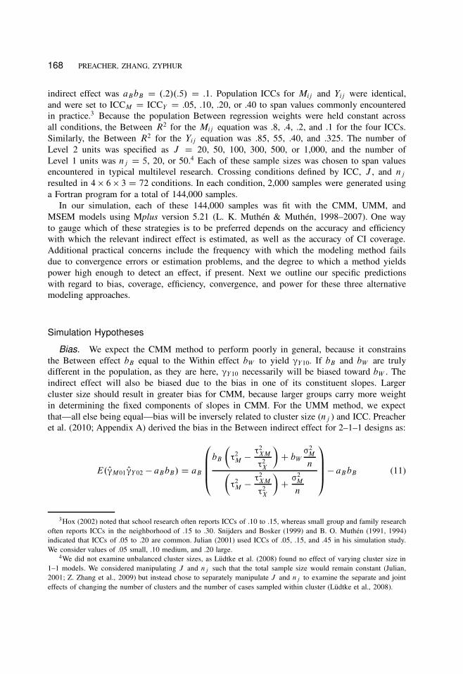
that—all else being equal—bias will be inversely related to cluster size (nj ) and ICC. Preacher
et al. (2010; Appendix A) derived the bias in the Between indirect effect for 2–1–1 designs as:
E. O”M01 O”Y 02 � aBbB/ D aB
0
B
B
B
@
bB
�
£2M �
£2XM
£2X
�
C bW
¢2M
n�
£2M �
£2XM
£2X
�
C¢2
M
n
1
C
C
C
A
� aB bB (11)
3Hox (2002) noted that school research often reports ICCs of .10 to .15, whereas small group and family research
often reports ICCs in the neighborhood of .15 to .30. Snijders and Bosker (1999) and B. O. Muthén (1991, 1994)
indicated that ICCs of .05 to .20 are common. Julian (2001) used ICCs of .05, .15, and .45 in his simulation study.
We consider values of .05 small, .10 medium, and .20 large.4We did not examine unbalanced cluster sizes, as Lüdtke et al. (2008) found no effect of varying cluster size in
1–1 models. We considered manipulating J and nj such that the total sample size would remain constant (Julian,
2001; Z. Zhang et al., 2009) but instead chose to separately manipulate J and nj to examine the separate and joint
effects of changing the number of clusters and the number of cases sampled within cluster (Lüdtke et al., 2008).
Downloaded By: [University of Kansas] At: 20:23 14 April 2011
MULTILEVEL SEM FOR MEDIATION 169
where aB , bB , and bW are the true Between and Within effects, n is the common cluster size for
balanced designs, ¢2M is the Within residual variance associated with Mij , and £2
X , £2M , and £XM
are the Between variances and covariance of the subscripted variables. The only quantities in
Equation 11 that are varied in the simulation are ¢2M and n. As ICCM increases, ¢2
M decreases.
As n increases and ¢2M decreases, the ratio ¢2
M =n tends toward zero, reducing the degree to
which bW biases the Between indirect effect. We expect little bias for the MSEM method
because it corresponds closely to the model used to generate the data. Overall, we expect
the UMM method to outperform CMM (Z. Zhang et al., 2009), and we expect MSEM to
outperform both CMM and UMM. In the simulation, bias is assessed using relative percentage
bias (RPB), computed as follows for the CMM, UMM, and MSEM strategies:
RPBCMM D 100Œ. O”M01 O”Y 10 � aB bB/=aBbB �%
RPBUMM D 100Œ. O”M01 O”Y 02 � aBbB /=aBbB �%
RPBMSEM D 100Œ.O“MXO“YM � aBbB/=aB bB �%
(12)
Confidence interval coverage. We expect MSEM to outperform both CMM and UMM
in reaching the nominal target coverage rate of .95 in all conditions—it is expected to yield the
least bias, leading to CIs that are more closely centered over the population indirect effect.5
Moreover, UMM is expected to outperform CMM because CMM is expected to yield more
biased indirect effects (Z. Zhang et al., 2009). We expect that the number of clusters will
influence CI coverage for CMM and UMM. Holding nj constant, increasing the number of
clusters increases the total sample size. This will increase precision and reduce CI width, which
in turn reduces coverage for biased effects. Coverage for CMM should improve with increasing
ICC because larger ICC corresponds to greater reliability for the cluster-level components of
Mij and Yij . Coverage is determined by noting the proportion of trials in which the 95% CI
for the Between indirect effect included the population (data-generating) value of aBbB .
Efficiency. Besides involving the estimation of more parameters, MSEM treats the Be-
tween components of Mij and Yij as latent, which leads to greater uncertainty in the estimation
of cluster-level structural parameters (Lüdtke et al., 2008). In addition, the near-singularity of
Between covariance matrices when ICC is very low might lead to unstable estimation and
consequently greater variability. However, Lüdtke et al. (2008) hypothesized, and found, that
MSEM was asymptotically the most efficient method if the model is correctly specified and
data are collected from a sufficiently large number of groups. We thus expect more efficient
estimation of the Between effect in the MSEM strategy relative to the UMM strategy if ICC
and the number of groups become sufficiently large. We have no specific prediction about
whether UMM or CMM will show more efficient estimation of the Between indirect effect.
We surmise that efficiency will improve as both Between and Within sample sizes and ICC
5The CIs we used are based on the multivariate delta method and incorrectly assume the indirect effect to be
normally distributed, and therefore symmetric about the point estimate. Because indirect effects typically are not
normally distributed in small samples, we expect coverage to be a little lower than .95 even under the best of
circumstances. Whereas this kind of CI suffices for comparing methods in a simulation, in practice we recommend
using a different kind of CI that does not assume the indirect effect to be symmetrically distributed (see Discussion).
Downloaded By: [University of Kansas] At: 20:23 14 April 2011
170 PREACHER, ZHANG, ZYPHUR
increase, simply because CI width is mostly a function of sample size and variability. We
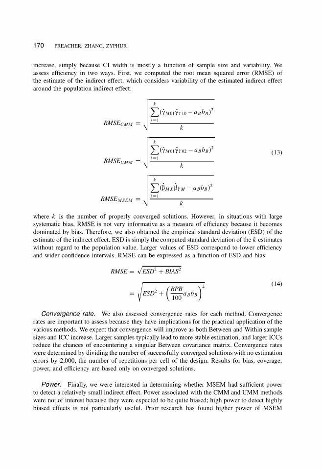
assess efficiency in two ways. First, we computed the root mean squared error (RMSE) of
the estimate of the indirect effect, which considers variability of the estimated indirect effect
around the population indirect effect:
RMSECMM D
v
u
u
u
u
t
kX
iD1
. O”M01 O”Y 10 � aB bB/2
k
RMSEUMM D
v
u
u
u
u
t
kX
iD1
. O”M01 O”Y 02 � aBbB/2
k
RMSEMSEM D
v
u
u
u
u
t
kX
iD1
.O“MXO“YM � aBbB/2
k
(13)
where k is the number of properly converged solutions. However, in situations with large
systematic bias, RMSE is not very informative as a measure of efficiency because it becomes
dominated by bias. Therefore, we also obtained the empirical standard deviation (ESD) of the
estimate of the indirect effect. ESD is simply the computed standard deviation of the k estimates
without regard to the population value. Larger values of ESD correspond to lower efficiency
and wider confidence intervals. RMSE can be expressed as a function of ESD and bias:
RMSE Dp
ESD2 C BIAS2
D
s
ESD2 C
�
RPB
100aBbB
�2 (14)
Convergence rate. We also assessed convergence rates for each method. Convergence
rates are important to assess because they have implications for the practical application of the
various methods. We expect that convergence will improve as both Between and Within sample
sizes and ICC increase. Larger samples typically lead to more stable estimation, and larger ICCs
reduce the chances of encountering a singular Between covariance matrix. Convergence rates
were determined by dividing the number of successfully converged solutions with no estimation
errors by 2,000, the number of repetitions per cell of the design. Results for bias, coverage,
power, and efficiency are based only on converged solutions.
Power. Finally, we were interested in determining whether MSEM had sufficient power
to detect a relatively small indirect effect. Power associated with the CMM and UMM methods
were not of interest because they were expected to be quite biased; high power to detect highly
biased effects is not particularly useful. Prior research has found higher power of MSEM
Downloaded By: [University of Kansas] At: 20:23 14 April 2011
MULTILEVEL SEM FOR MEDIATION 171
TABLE 1
Percentage Relative Bias of the Between Indirect Effect in 2–1–1 Models
for CMM, UMM, and MSEM Strategies
CMM UMM MSEM
J nj ¡ D :05 ¡ D :10 ¡ D :20 ¡ D :40 ¡ D :05 ¡ D :10 ¡ D :20 ¡ D :40 ¡ D :05 ¡ D :10 ¡ D :20 ¡ D :40
20 5 �60.34 �57.24 �53.27 �49.72 �57.80 �44.61 �31.76 �15.01 �38.16 �15.87 8.02 12.04
50 5 �60.38 �56.87 �53.07 �50.88 �56.84 �45.63 �30.01 �16.76 �19.02 �6.25 10.30 .91
100 5 �59.45 �56.44 �53.55 �49.11 �55.79 �44.08 �30.31 �13.91 �17.45 6.92 4.58 2.60
300 5 �59.66 �57.04 �54.24 �49.98 �57.21 �45.63 �31.07 �15.15 �17.10 6.38 .26 .21
500 5 �59.63 �56.84 �53.44 �49.95 �57.08 �44.82 �29.75 �14.93 �17.02 6.03 1.37 .29
1,000 5 �59.41 �56.94 �53.53 �50.23 �57.11 �44.88 �29.96 �15.26 �15.55 3.42 .50 �.17
20 20 �60.07 �58.55 �57.05 �56.51 �50.80 �28.10 �10.34 �5.12 �30.57 9.50 9.53 1.19
50 20 �59.40 �58.27 �57.18 �55.89 �49.48 �26.15 �12.69 �2.47 �19.40 6.65 1.08 2.88
100 20 �59.43 �58.07 �56.96 �57.01 �49.64 �25.82 �12.42 �5.33 �8.92 2.95 .28 �.43
300 20 �59.33 �58.21 �57.35 �56.81 �49.81 �25.75 �12.14 �4.16 3.85 1.11 .12 .58
500 20 �59.34 �58.42 �57.37 �56.86 �49.54 �26.00 �12.29 �4.82 6.07 .23 �.15 �.17
1,000 20 �59.32 �58.16 �57.28 �56.80 �49.44 �25.79 �12.13 �4.45 5.32 .18 �.08 .20
20 50 �59.15 �59.00 �58.99 �58.88 �40.40 �14.20 �4.71 �1.26 �2.39 7.88 3.58 1.52
50 50 �59.30 �59.05 �58.09 �59.28 �39.65 �14.80 �3.01 �4.49 6.06 1.65 3.35 �2.36
100 50 �59.32 �59.02 �58.96 �58.81 �39.14 �14.49 �6.44 �2.01 7.70 .23 �.75 .04
300 50 �59.62 �58.98 �58.87 �58.90 �39.43 �14.10 �5.81 �1.94 3.19 .05 �.29 .04
500 50 �59.61 �58.92 �58.59 �58.72 �39.43 �13.82 �5.16 �2.29 1.63 .18 .35 �.34
1,000 50 �59.56 �58.96 �58.77 �58.72 �39.50 �13.66 �5.39 �1.77 .47 .39 .09 .18
Note. J D number of clusters; nj D within-cluster sample size; ¡ D population intraclass correlation; CMM D conflated
multilevel modeling; UMM D unconflated multilevel modeling; MSEM D multilevel structural equation modeling.
than MLM in detecting cross-level interactions in multilevel data (e.g., D. Zhang & Willson,
2006). However, it remains a question whether power will be adequate using MSEM to detect
multilevel mediation. On one hand, we expected more sampling variability in the point estimate
of the indirect effect in MSEM (which compromises power); on the other hand, we expected
MSEM to demonstrate less bias (which should enhance power). Therefore, a secondary goal
was to determine whether or not MSEM had adequate power to detect a small indirect effect.
To obtain power, we determined the proportion of the converged trials within each cell in
which the null hypothesis of no mediation was rejected at ’ D :05. We used delta method
approximate standard errors to conduct Wald tests (Sobel, 1982). Whereas we would not
recommend this method in practice because of its known limitations (Preacher & Hayes, 2004,
2008a, 2008b), we use it here because it is simple and straightforward, and the simulation
would take a dramatically longer time if more appropriate bootstrapping methods were used.
This test still permits fair comparisons among CMM, UMM, and MSEM.
Results
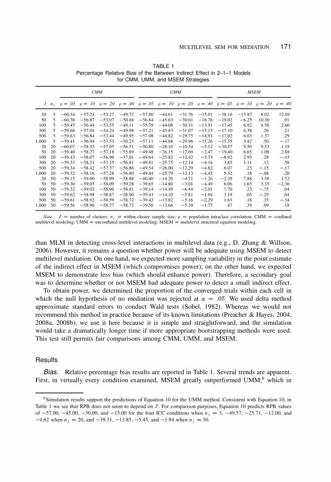
Bias. Relative percentage bias results are reported in Table 1. Several trends are apparent.
First, in virtually every condition examined, MSEM greatly outperformed UMM,6 which in
6Simulation results support the predictions of Equation 10 for the UMM method. Consistent with Equation 10, in
Table 1 we see that RPB does not seem to depend on J . For comparison purposes, Equation 10 predicts RPB values
of �57.00, �45.00, �30.00, and �15.00 for the four ICC conditions when nj D 5, �49.57, �25.71, �12.00, and
�4.62 when nj D 20, and �39.31, �13.85, �5.45, and �1.94 when nj D 50.
Downloaded By: [University of Kansas] At: 20:23 14 April 2011
172 PREACHER, ZHANG, ZYPHUR
TABLE 2
Confidence Interval Coverage for the Between Indirect Effect in 2–1–1 Models
for CMM, UMM, and MSEM Strategies
CMM UMM MSEM
J nj ¡ D :05 ¡ D :10 ¡ D :20 ¡ D :40 ¡ D :05 ¡ D :10 ¡ D :20 ¡ D :40 ¡ D :05 ¡ D :10 ¡ D :20 ¡ D :40
20 5 .460 .491 .567 .643 .603 .699 .778 .830 .920 .905 .902 .880
50 5 .168 .255 .357 .486 .492 .621 .754 .857 .929 .908 .914 .910
100 5 .032 .062 .133 .313 .310 .502 .703 .880 .951 .931 .926 .924
300 5 .000 .000 .001 .022 .017 .129 .473 .850 .964 .953 .947 .944
500 5 .000 .000 .000 .002 .001 .031 .335 .799 .967 .956 .943 .939
1,000 5 .000 .000 .000 .000 .000 .000 .085 .680 .971 .965 .950 .951
20 20 .124 .191 .340 .496 .652 .774 .831 .863 .920 .888 .863 .880
50 20 .003 .019 .083 .248 .528 .756 .863 .908 .923 .927 .915 .916
100 20 .001 .001 .009 .051 .315 .723 .889 .913 .948 .938 .946 .921
300 20 .001 .000 .000 .000 .025 .457 .848 .922 .956 .957 .947 .933
500 20 .001 .000 .000 .000 .002 .264 .777 .921 .967 .941 .950 .937
1,000 20 .001 .000 .000 .000 .000 .064 .686 .918 .965 .951 .946 .942
20 50 .029 .083 .218 .398 .736 .831 .859 .869 .903 .892 .876 .877
50 50 .004 .002 .027 .137 .642 .858 .892 .899 .949 .916 .905 .905
100 50 .003 .000 .001 .019 .468 .840 .900 .927 .952 .936 .920 .938
300 50 .000 .000 .000 .000 .093 .763 .913 .939 .957 .948 .950 .942
500 50 .000 .000 .000 .000 .012 .674 .911 .937 .957 .941 .944 .943
1,000 50 .000 .000 .000 .000 .000 .475 .883 .938 .956 .955 .947 .951
Note. J D number of clusters; nj D within-cluster sample size; ¡ D population intraclass correlation; CMM D conflated
multilevel modeling; UMM D unconflated multilevel modeling; MSEM D multilevel structural equation modeling.
turn outperformed CMM. The degree of bias was inversely related to ICC and within-cluster
sample size for UMM and MSEM. As predicted, bias increased with cluster size for CMM,
with the difference in bias across cluster sizes becoming more pronounced at higher ICCs. For
the MSEM approach, bias was inversely related to number of clusters to a small degree. CMM
showed acceptably small bias under no conditions, UMM showed acceptably small bias only
with high ICC (.40 when nj D 20 and .20 in some nj D 50 conditions) and larger within-cluster
sample sizes, and MSEM showed acceptably small bias in most conditions. When unacceptable
bias was found, it was almost always negative. Bias was dramatically lower for MSEM than
for CMM and UMM in most conditions examined, although not eliminated. Unacceptable bias
was found for MSEM, particularly when group size was small (5) and when ICC was low
(.05 or .10). Assuming that researchers adhere to common sample size recommendations for
MLM (Hox & Maas, 2001; Maas & Hox, 2005; Snijders & Bosker, 1999) when using MSEM
(discussed later), these problems are minimized.
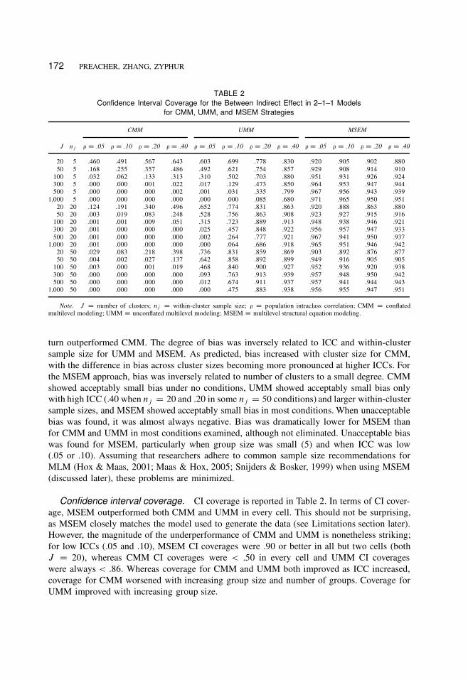
Confidence interval coverage. CI coverage is reported in Table 2. In terms of CI cover-
age, MSEM outperformed both CMM and UMM in every cell. This should not be surprising,
as MSEM closely matches the model used to generate the data (see Limitations section later).
However, the magnitude of the underperformance of CMM and UMM is nonetheless striking;
for low ICCs (.05 and .10), MSEM CI coverages were .90 or better in all but two cells (both
J D 20), whereas CMM CI coverages were < .50 in every cell and UMM CI coverages
were always < .86. Whereas coverage for CMM and UMM both improved as ICC increased,
coverage for CMM worsened with increasing group size and number of groups. Coverage for
UMM improved with increasing group size.
Downloaded By: [University of Kansas] At: 20:23 14 April 2011
MULTILEVEL SEM FOR MEDIATION 173
TABLE 3
Empirical Standard Deviation of the Estimate of the Between Indirect Effect in 2–1–1 Models
for CMM, UMM, and MSEM Strategies
CMM UMM MSEM
J nj ¡ D :05 ¡ D :10 ¡ D :20 ¡ D :40 ¡ D :05 ¡ D :10 ¡ D :20 ¡ D :40 ¡ D :05 ¡ D :10 ¡ D :20 ¡ D :40
20 5 .032 .037 .041 .052 .064 .066 .074 .096 .250 .251 .242 .165
50 5 .019 .020 .023 .029 .033 .037 .041 .054 .169 .170 .114 .070
100 5 .013 .014 .017 .020 .023 .025 .029 .037 .150 .143 .062 .047
300 5 .007 .008 .009 .011 .012 .014 .015 .020 .135 .070 .029 .024
500 5 .006 .006 .007 .009 .010 .011 .012 .016 .144 .049 .023 .020
1,000 5 .004 .004 .005 .006 .007 .007 .009 .011 .140 .031 .016 .013
20 20 .016 .021 .027 .037 .053 .058 .075 .093 .181 .151 .110 .103
50 20 .010 .012 .015 .020 .031 .035 .041 .051 .153 .077 .051 .055
100 20 .007 .008 .011 .015 .021 .022 .027 .037 .125 .042 .032 .040
300 20 .004 .005 .006 .009 .012 .013 .015 .021 .101 .022 .018 .023
500 20 .003 .004 .005 .006 .009 .010 .012 .016 .071 .017 .014 .017
1,000 20 .003 .003 .003 .005 .006 .007 .009 .011 .047 .012 .010 .012
20 50 .012 .016 .022 .032 .051 .058 .072 .092 .186 .099 .084 .096
50 50 .007 .009 .014 .019 .029 .033 .041 .053 .121 .045 .045 .054
100 50 .006 .007 .010 .013 .021 .023 .028 .036 .082 .029 .030 .036
300 50 .003 .004 .005 .008 .012 .013 .015 .020 .038 .016 .017 .021
500 50 .002 .003 .004 .006 .009 .010 .012 .015 .028 .013 .013 .016
1,000 50 .001 .002 .003 .004 .006 .007 .009 .011 .019 .009 .009 .012
Note. J D number of clusters; nj D within-cluster sample size; ¡ D population intraclass correlation; CMM D conflated
multilevel modeling; UMM D unconflated multilevel modeling; MSEM D multilevel structural equation modeling.
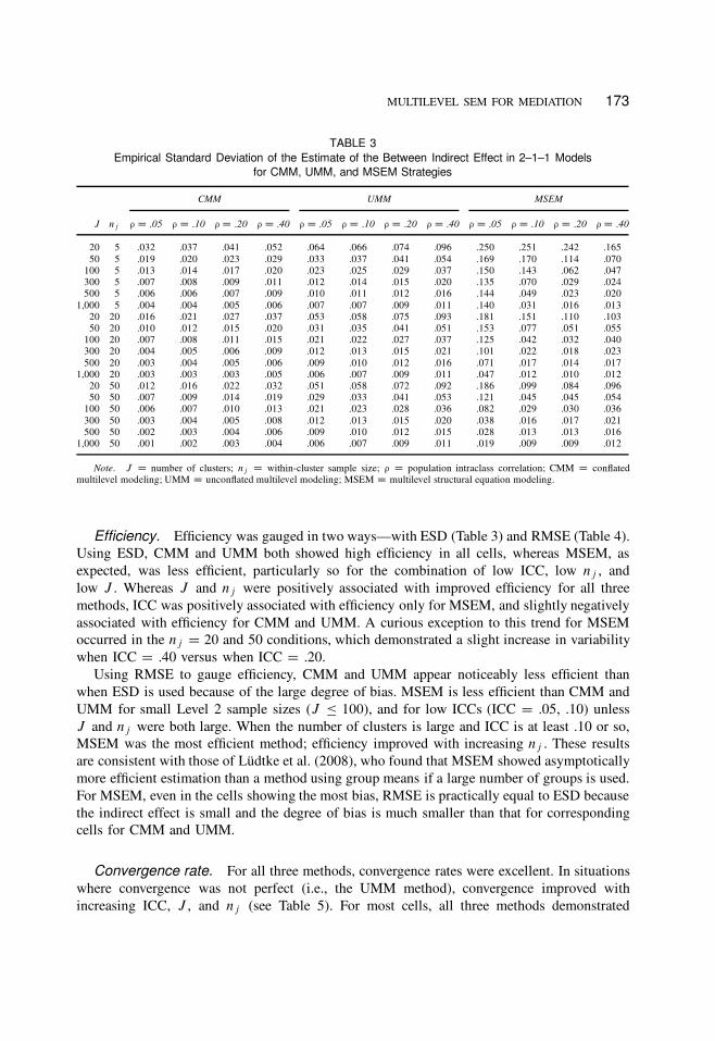
Efficiency. Efficiency was gauged in two ways—with ESD (Table 3) and RMSE (Table 4).
Using ESD, CMM and UMM both showed high efficiency in all cells, whereas MSEM, as
expected, was less efficient, particularly so for the combination of low ICC, low nj , and
low J . Whereas J and nj were positively associated with improved efficiency for all three
methods, ICC was positively associated with efficiency only for MSEM, and slightly negatively
associated with efficiency for CMM and UMM. A curious exception to this trend for MSEM
occurred in the nj D 20 and 50 conditions, which demonstrated a slight increase in variability
when ICC D .40 versus when ICC D .20.
Using RMSE to gauge efficiency, CMM and UMM appear noticeably less efficient than
when ESD is used because of the large degree of bias. MSEM is less efficient than CMM and
UMM for small Level 2 sample sizes (J � 100), and for low ICCs (ICC D .05, .10) unless
J and nj were both large. When the number of clusters is large and ICC is at least .10 or so,
MSEM was the most efficient method; efficiency improved with increasing nj . These results
are consistent with those of Lüdtke et al. (2008), who found that MSEM showed asymptotically
more efficient estimation than a method using group means if a large number of groups is used.
For MSEM, even in the cells showing the most bias, RMSE is practically equal to ESD because
the indirect effect is small and the degree of bias is much smaller than that for corresponding
cells for CMM and UMM.
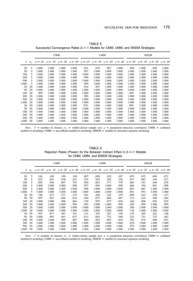
Convergence rate. For all three methods, convergence rates were excellent. In situations
where convergence was not perfect (i.e., the UMM method), convergence improved with
increasing ICC, J , and nj (see Table 5). For most cells, all three methods demonstrated
Downloaded By: [University of Kansas] At: 20:23 14 April 2011
174 PREACHER, ZHANG, ZYPHUR
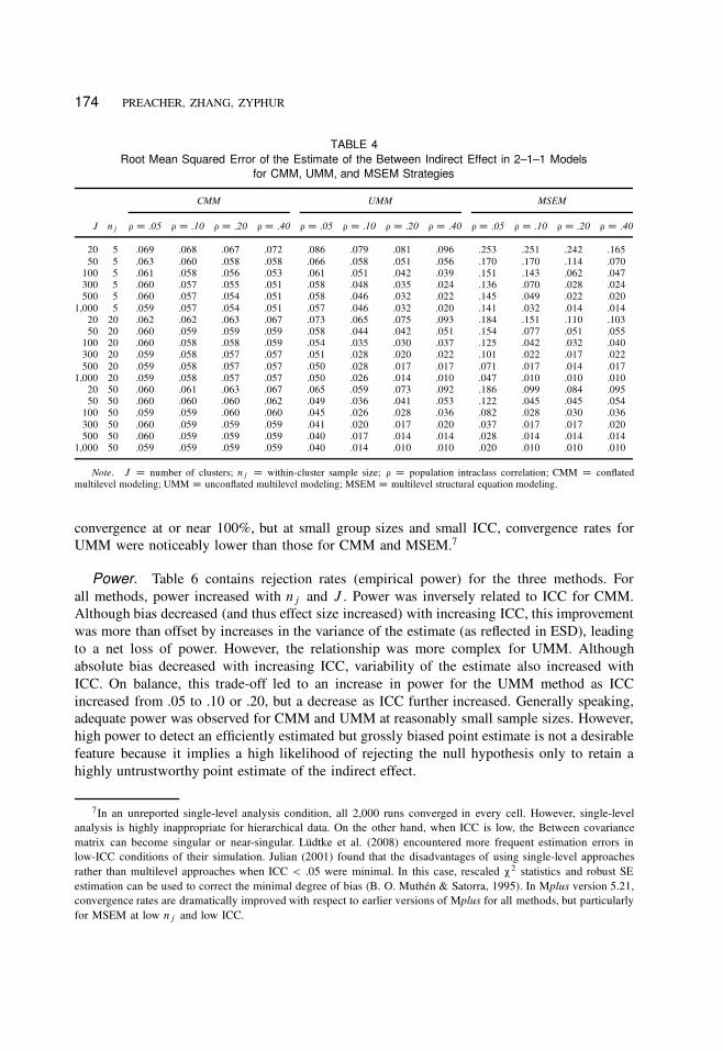
TABLE 4
Root Mean Squared Error of the Estimate of the Between Indirect Effect in 2–1–1 Models
for CMM, UMM, and MSEM Strategies
CMM UMM MSEM
J nj ¡ D :05 ¡ D :10 ¡ D :20 ¡ D :40 ¡ D :05 ¡ D :10 ¡ D :20 ¡ D :40 ¡ D :05 ¡ D :10 ¡ D :20 ¡ D :40
20 5 .069 .068 .067 .072 .086 .079 .081 .096 .253 .251 .242 .165
50 5 .063 .060 .058 .058 .066 .058 .051 .056 .170 .170 .114 .070
100 5 .061 .058 .056 .053 .061 .051 .042 .039 .151 .143 .062 .047
300 5 .060 .057 .055 .051 .058 .048 .035 .024 .136 .070 .028 .024
500 5 .060 .057 .054 .051 .058 .046 .032 .022 .145 .049 .022 .020
1,000 5 .059 .057 .054 .051 .057 .046 .032 .020 .141 .032 .014 .014
20 20 .062 .062 .063 .067 .073 .065 .075 .093 .184 .151 .110 .103
50 20 .060 .059 .059 .059 .058 .044 .042 .051 .154 .077 .051 .055
100 20 .060 .058 .058 .059 .054 .035 .030 .037 .125 .042 .032 .040
300 20 .059 .058 .057 .057 .051 .028 .020 .022 .101 .022 .017 .022
500 20 .059 .058 .057 .057 .050 .028 .017 .017 .071 .017 .014 .017
1,000 20 .059 .058 .057 .057 .050 .026 .014 .010 .047 .010 .010 .010
20 50 .060 .061 .063 .067 .065 .059 .073 .092 .186 .099 .084 .095
50 50 .060 .060 .060 .062 .049 .036 .041 .053 .122 .045 .045 .054
100 50 .059 .059 .060 .060 .045 .026 .028 .036 .082 .028 .030 .036
300 50 .060 .059 .059 .059 .041 .020 .017 .020 .037 .017 .017 .020
500 50 .060 .059 .059 .059 .040 .017 .014 .014 .028 .014 .014 .014
1,000 50 .059 .059 .059 .059 .040 .014 .010 .010 .020 .010 .010 .010
Note. J D number of clusters; nj D within-cluster sample size; ¡ D population intraclass correlation; CMM D conflated
multilevel modeling; UMM D unconflated multilevel modeling; MSEM D multilevel structural equation modeling.
convergence at or near 100%, but at small group sizes and small ICC, convergence rates for
UMM were noticeably lower than those for CMM and MSEM.7
Power. Table 6 contains rejection rates (empirical power) for the three methods. For
all methods, power increased with nj and J . Power was inversely related to ICC for CMM.
Although bias decreased (and thus effect size increased) with increasing ICC, this improvement
was more than offset by increases in the variance of the estimate (as reflected in ESD), leading
to a net loss of power. However, the relationship was more complex for UMM. Although
absolute bias decreased with increasing ICC, variability of the estimate also increased with
ICC. On balance, this trade-off led to an increase in power for the UMM method as ICC
increased from .05 to .10 or .20, but a decrease as ICC further increased. Generally speaking,
adequate power was observed for CMM and UMM at reasonably small sample sizes. However,
high power to detect an efficiently estimated but grossly biased point estimate is not a desirable
feature because it implies a high likelihood of rejecting the null hypothesis only to retain a
highly untrustworthy point estimate of the indirect effect.
7In an unreported single-level analysis condition, all 2,000 runs converged in every cell. However, single-level
analysis is highly inappropriate for hierarchical data. On the other hand, when ICC is low, the Between covariance
matrix can become singular or near-singular. Lüdtke et al. (2008) encountered more frequent estimation errors in
low-ICC conditions of their simulation. Julian (2001) found that the disadvantages of using single-level approaches
rather than multilevel approaches when ICC < .05 were minimal. In this case, rescaled ¦2 statistics and robust SE
estimation can be used to correct the minimal degree of bias (B. O. Muthén & Satorra, 1995). In Mplus version 5.21,
convergence rates are dramatically improved with respect to earlier versions of Mplus for all methods, but particularly
for MSEM at low nj and low ICC.
Downloaded By: [University of Kansas] At: 20:23 14 April 2011
MULTILEVEL SEM FOR MEDIATION 175
TABLE 5
Successful Convergence Rates 2–1–1 Models for CMM, UMM, and MSEM Strategies
CMM UMM MSEM
J nj ¡ D :05 ¡ D :10 ¡ D :20 ¡ D :40 ¡ D :05 ¡ D :10 ¡ D :20 ¡ D :40 ¡ D :05 ¡ D :10 ¡ D :20 ¡ D :40
20 5 1.000 1.000 1.000 1.000 .931 .970 .997 1.000 .999 1.000 .999 1.000
50 5 1.000 1.000 1.000 1.000 .997 1.000 1.000 1.000 1.000 1.000 1.000 1.000
100 5 1.000 1.000 1.000 1.000 1.000 1.000 1.000 1.000 1.000 1.000 1.000 1.000
300 5 1.000 1.000 1.000 1.000 .999 1.000 1.000 1.000 1.000 1.000 1.000 1.000
500 5 1.000 1.000 1.000 1.000 1.000 1.000 1.000 1.000 1.000 1.000 1.000 1.000
1,000 5 1.000 1.000 1.000 1.000 .999 1.000 1.000 1.000 1.000 1.000 1.000 1.000
20 20 1.000 1.000 1.000 1.000 .954 .997 1.000 1.000 1.000 1.000 1.000 1.000
50 20 1.000 1.000 1.000 1.000 1.000 1.000 1.000 1.000 1.000 1.000 1.000 1.000
100 20 .999 1.000 1.000 1.000 1.000 1.000 1.000 1.000 .999 1.000 1.000 1.000
300 20 1.000 1.000 1.000 1.000 .999 1.000 1.000 1.000 1.000 1.000 1.000 1.000
500 20 1.000 1.000 1.000 1.000 1.000 1.000 1.000 1.000 1.000 1.000 1.000 1.000
1,000 20 1.000 1.000 1.000 1.000 1.000 1.000 1.000 1.000 1.000 1.000 1.000 1.000
20 50 1.000 1.000 1.000 1.000 .978 1.000 1.000 1.000 .999 1.000 1.000 1.000
50 50 1.000 1.000 1.000 1.000 1.000 1.000 1.000 1.000 1.000 1.000 1.000 1.000
100 50 1.000 1.000 1.000 1.000 1.000 1.000 1.000 1.000 1.000 1.000 1.000 1.000
300 50 1.000 1.000 1.000 1.000 1.000 1.000 1.000 1.000 1.000 1.000 1.000 1.000
500 50 1.000 1.000 1.000 1.000 1.000 1.000 1.000 1.000 1.000 1.000 1.000 1.000
1,000 50 1.000 1.000 1.000 1.000 1.000 1.000 1.000 1.000 1.000 1.000 1.000 1.000
Note. J D number of clusters; nj D within-cluster sample size; ¡ D population intraclass correlation; CMM D conflated
multilevel modeling; UMM D unconflated multilevel modeling; MSEM D multilevel structural equation modeling.
TABLE 6
Rejection Rates (Power) for the Between Indirect Effect in 2–1–1 Models
for CMM, UMM, and MSEM Strategies
CMM UMM MSEM
J nj ¡ D :05 ¡ D :10 ¡ D :20 ¡ D :40 ¡ D :05 ¡ D :10 ¡ D :20 ¡ D :40 ¡ D :05 ¡ D :10 ¡ D :20 ¡ D :40
20 5 .184 .189 .190 .140 .087 .098 .102 .107 .035 .035 .049 .071
50 5 .622 .603 .558 .421 .225 .282 .365 .326 .037 .082 .146 .257
100 5 .965 .948 .897 .793 .504 .683 .777 .739 .065 .141 .466 .678
300 5 1.000 1.000 1.000 .998 .957 .995 1.000 .998 .066 .394 .983 .998
500 5 1.000 1.000 1.000 1.000 .998 1.000 1.000 1.000 .083 .687 1.000 1.000
1,000 5 1.000 1.000 1.000 1.000 1.000 1.000 1.000 1.000 .091 .953 1.000 1.000
20 20 .786 .673 .477 .315 .201 .268 .242 .159 .069 .162 .196 .147
50 20 .997 .967 .848 .634 .449 .675 .660 .497 .133 .414 .580 .484
100 20 1.000 1.000 .988 .864 .720 .959 .975 .830 .166 .808 .945 .825
300 20 1.000 1.000 1.000 .999 .993 1.000 1.000 .999 .240 .999 1.000 .999
500 20 1.000 1.000 1.000 1.000 1.000 1.000 1.000 1.000 .386 1.000 1.000 1.000
1,000 20 1.000 1.000 1.000 1.000 1.000 1.000 1.000 1.000 .738 1.000 1.000 1.000
20 50 .955 .817 .587 .391 .331 .382 .287 .194 .155 .305 .262 .188
50 50 1.000 .993 .901 .637 .613 .844 .752 .489 .225 .751 .725 .482
100 50 1.000 1.000 .989 .887 .860 .992 .983 .854 .392 .970 .980 .853
300 50 1.000 1.000 1.000 1.000 1.000 1.000 1.000 1.000 .828 1.000 1.000 1.000
500 50 1.000 1.000 1.000 1.000 1.000 1.000 1.000 1.000 .979 1.000 1.000 1.000
1,000 50 1.000 1.000 1.000 1.000 1.000 1.000 1.000 1.000 1.000 1.000 1.000 1.000
Note. J D number of clusters; nj D within-cluster sample size; ¡ D population intraclass correlation; CMM D conflated
multilevel modeling; UMM D unconflated multilevel modeling; MSEM D multilevel structural equation modeling.
Downloaded By: [University of Kansas] At: 20:23 14 April 2011
176 PREACHER, ZHANG, ZYPHUR
Power results for MSEM are complex. Power increased with both nj and J , and increased
with ICC in the small clusters (nj D 5) conditions. Power increased and then decreased with
ICC for the J D 20 through J D 500 conditions with larger clusters. That is, the ICC D
.40 conditions tended to be characterized by lower power than the ICC D .20 conditions for
the larger cluster size conditions. This decreased power is likely due to the slight upturn in
variability observed for these same cells, in terms of both ESD and RMSE. Overall, MSEM’s
power to detect a relatively small indirect effect of .1 was acceptable for ICC � .20 and
J � 300 when clusters were small .nj D 5/, for ICC � .10 and J � 100 when clusters
were larger .nj D 20/, and for ICC � .05 and J � 300 for the largest cluster size examined
.nj D 50/. It should be emphasized that power seems small in many of the conditions because
the true Between indirect effect is quite small (.1). As the size of the indirect effect increases,
power will increase.
Summary
We began this article with two goals. The first was to demonstrate that MSEM reduces bias in
Between indirect effects relative to more traditional MLM-based procedures using the popularly
examined 2–1–1 mediation model. It does so, and dramatically. In many cells of the design,
bias was negligible, particularly as ICC, J , and nj increased. In situations with low ICCs,
particularly ICC < .10, researchers should be aware that some bias still exists.
The second main goal was to evaluate the performance of MSEM in terms of CI coverage,
efficiency, and convergence using the 2–1–1 mediation model. MSEM performed very well,
in both an absolute sense and relative to CMM and UMM, in terms of achieving nominal CI
coverage, although coverage remained somewhat lower than .95 when the number of clusters
was small .J � 50/. In terms of efficiency, MSEM performed less well than competing MLM-
based methods in some conditions, but better than MLM-based methods when J , nj , and ICC
reached reasonably large values. In terms of convergence, all models performed well, even in
small sample size and low ICC conditions.
A secondary goal was to establish whether MSEM had sufficient power to be useful in
practice. We found that it did; if researchers adhere to sample size recommendations and have
high enough ICC (see Discussion and Preacher et al., 2010), then correctly rejecting the null
hypothesis is likely with MSEM.
On balance, the results of the simulation study illustrate advantages of using MSEM over
CMM and UMM for recovering the indirect effect when the indirect effect of interest exists
solely at the Between level. If even one of the variables involved in a mediation effect is a
Level 2 variable, then the indirect effect must exist at the Between level (Preacher et al., 2010).
MSEM showed dramatically less bias and better coverage than CMM and UMM, reaching
acceptable levels of each in all cases except those corresponding to sample sizes that have
been deemed too small for fitting multilevel models (e.g., Hox & Maas, 2001; Maas & Hox,
2005). The trade-off is that MSEM had worse efficiency for low ICC (particularly with small
clusters) compared to CMM and UMM. However, we emphasize that efficient estimation of a
strongly biased quantity is not only of little practical use, but is detrimental to a researcher’s
agenda. We replicated differences between CMM and UMM found in prior research (Z. Zhang
et al., 2009) such that, when Between and Within effects are of different magnitudes, the CMM
Downloaded By: [University of Kansas] At: 20:23 14 April 2011
MULTILEVEL SEM FOR MEDIATION 177
strategy conflates them. The UMM method separates these two conceptually different effects,
yet still exhibits nontrivial bias for the Between indirect effect in most examined conditions.
These findings, although limited to the 2–1–1 design and only one choice of population
parameter values, are expected to generalize to other multilevel mediation designs, such as the
1–1–1 design with fixed slopes and the 2–1–1 design with random slopes. To investigate the
latter claim, we reran the entire simulation with a random slope for the Within Mij ! Yij
effect. In brief, the same results were found; the presence of a random slope in the model
does not seem to seriously impede processing time or convergence rates for MSEM, and bias,
coverage, and power were similar to those reported for corresponding cells in our fixed-slope
simulation. We noticed a severe drop in convergence rates for UMM in the smallest sample
size conditions when the Within slope is random—another reason to prefer MSEM. Detailed
results on the 2–1–1 model with random 1–1 slopes are available at the first author’s Web site.
DISCUSSION
We have shown via simulation that the MSEM approach dramatically reduces bias due to the
conflation of between- and within-group effects and unreliable cluster means that characterize
existing models for multilevel mediation under the MLM framework, in exchange for modest
decreases in efficiency under conditions of few clusters, small clusters, and low ICC. Nev-
ertheless, the absolute degree of estimation variability in MSEM was not serious enough to
compromise power.
The MSEM approach for multilevel mediation analysis is also viable at a practical level.
The methods we described are available in recent versions of Mplus, and we provide online
syntax8 for the model used in our simulation as well as for several other models. Users merely
need to modify and customize our syntax to suit their own needs.
Limitations
Our study has some limitations that deserve mention. First, we examined one particular
multilevel model (i.e., 2–1–1) under a restricted set of circumstances (e.g., normally distributed
variables, no random slopes). As with most simulation studies, results are limited to the
conditions examined. Nonetheless, our conclusions are expected to generalize to any MSEM
model with similar relationships among variables. As discussed earlier, the entire simulation
was rerun with a random Within slope and essentially the same results were found.
We also reran the entire simulation setting bW D bB D :5 to observe results when no
contextual effect is present. In terms of ESD, MSEM performed slightly better than when
bW ¤ bB , and CMM and UMM performed slightly worse. All three methods performed
slightly better in terms of RMSE and did well in terms of CI coverage, with CMM and
UMM performance rapidly deteriorating as bW departs from bB . Empirical power for the
three methods was essentially the same as in the primary simulation, except that power is
higher overall when bW D bB . A large increase in power was observed for CMM and UMM
because the b coefficient is no longer a weighted average of .2 and .5 (for CMM) or biased
8See http://www.quantpsy.org/
Downloaded By: [University of Kansas] At: 20:23 14 April 2011
178 PREACHER, ZHANG, ZYPHUR
toward .2 from .5 (for UMM) when bW D bB , and the large differences in bias observed
for CMM/UMM versus MSEM in the first simulation are no longer apparent when bW D bB .
However, bias quickly accumulates for CMM and UMM when bB ¤ bW . These results support
and complement findings from the original simulation. Results from all three simulation studies
can be found at the first author’s Web site.
Second, we did little to highlight modeling extensions that are more feasible within the
MSEM framework than the MLM framework. For example, MSEM makes it easy to specify
mediation models involving more than one mediator, accommodates longer causal chains with
Level 2 mediators or Level 2 dependent variables (e.g., Vandenberg, Richardson, & Eastman,
1999), and permits the inclusion of latent variables with multiple observed indicators. Every
additional dependent variable adds a layer of complexity in the MLM framework because
it often requires significant data management (depending on the specific software used), but
adding additional dependent variables in MSEM is straightforward. Whereas the ability to
specify latent variables is one of the most attractive features of MSEM, the ability to use latent
variables in MLM is somewhat limited (Goldstein, Kounali, & Robinson, 2008; Raudenbush,
Rowan, & Kang, 1991).
Third, we limited attention to models featuring only continuous, normally distributed ob-
served variables. For censored, categorical, and count variables, numerical integration often will
be required. It is unknown how the methods that were compared in our simulation will fare
with other types of data. Future simulations are needed to address how MSEM will function
in relation to alternative methods under these circumstances.
Fourth, we assumed a sampling ratio of 0 for all the Level 2 units for the purpose of
simplicity. In doing so, we assumed that the average researcher would be interested in fitting
models to data gathered via two-stage random sampling—a common assumption in most MLM
applications. In two-stage random sampling, clusters are assumed to have been randomly
sampled from a larger population of clusters, and individuals within clusters are assumed
to have been sampled from a larger population of such individuals. The reality, of course,
could be very different (as when data are collected from dyads). We are careful to limit our
conclusions to cases with low sampling ratios. If the sampling ratio is high (i.e., when the
cluster size is finite and we select a large proportion of individuals from each cluster), then the
manifest group mean might be a good proxy for group standing (for continuous variables) or
group composition (for dichotomous variables such as gender), as described by Lüdtke et al.
(2008).
Fifth, we limited our attention to the MSEM method of B. O. Muthén and Asparouhov (2008)
because of its generality, efficiency, and ease of implementation. However, it is not the only
method of combining latent variable structural equation modeling with MLM. There are many
such methods, each with advantages and disadvantages relative to other methods. The method
we used has at least three important limitations that restrict its application in practice. First,
although extensions to three levels are possible in some cases, the method is mainly restricted to
two-level models. Other approaches, such as the MSEM method employed in the GLLAMM
module for Stata (Rabe-Hesketh, Skrondal, & Pickles, 2004) and the method described by
Goldstein et al. (2008) for incorporating measurement error in multilevel models, can be
applied to data hierarchies with three or more levels (implemented in MLwiN). Second, the
method we used does not accommodate cross-classified or multiple-membership models. Third,
restricted maximum likelihood (REML) yields better estimates of random effect variances
Downloaded By: [University of Kansas] At: 20:23 14 April 2011
MULTILEVEL SEM FOR MEDIATION 179
and covariances than maximum likelihood (ML), but REML is not implemented in Mplus.
For model comparison purposes, we used ML estimation via an accelerated E-M algorithm
implemented by default in Mplus for all CMM, UMM, and MSEM models. We ran separate
tests with REML on the simulated data for CMM and UMM models and found that REML
and ML provided highly similar indirect effects. Other packages, such as MLwiN, GLLAMM,
HLM, and SAS PROC MIXED, offer REML as an option, and can fit models to data with
more than two hierarchical levels. Comparison of the various methods of combining structural
equation modeling and MLM lies beyond the scope of this study. We expect that future
advances in MLM software packages will permit a greater range of models. Future work
should be undertaken to investigate the feasibility of alternative methods for mediation analysis
in multilevel designs.
Finally, it might be objected that our data-generating model was equivalent to the model that
is fit in the MSEM approach, and that this biased the results in favor of MSEM. Clearly, if the
model used to generate the data is one of the models being compared using those very data, it
stands a good chance of outperforming its rivals. We appreciate this objection, but have several
responses. First, we wanted to generate data that conformed to the assumptions underlying
most multilevel models, that is, two-stage random sampling, and also had to build in realistic
differences in the Between and Within effects of Mij on Yij to show how various methods
did or did not address this difference. One reasonable way to do this was to use a multivariate
linear model with a structure that displayed the desired characteristics. Second, we note that
simply because a model is used to generate data does not guarantee that it will outperform
its competitors in every respect when fit to those data. Indeed, we found that even though our
data-generation algorithm was consistent with the MSEM approach, MSEM was not always as
efficient as competing methods (using the ESD and RMSE measures of efficiency). Third, even
though we expected MSEM to outperform the CMM and UMM methods in a number of ways,
it was of interest to determine by how much it would outperform them. If MSEM performed
only marginally better than other, simpler methods, it could be argued that a modeling strategy
like MSEM, which is complex and implemented in only a few software packages, does not
have substantial advantages. However, we found that the performance gap was quite large,
justifying the use of MSEM.
Recommendations
Sample size. The results of our simulation extend prior MSEM sample size recommen-
dations to B. O. Muthén and Asparouhov’s (2008) MSEM model in the context of mediation.
From our results, it is clear that increasing nj and J leads to more efficient estimation and
substantially lower bias. Cluster sizes of at least 20 (for small ICCs) were necessary to avoid
unacceptable bias. CI coverage was acceptable at all sample sizes examined. We recommend
that researchers consider these findings when planning studies with similar designs, and that
future research on MSEM for multilevel mediation consider a range of effect sizes to facilitate
making further recommendations.
Confidence intervals and significance testing. Mplus provides 95% CIs obtained using
the delta method. We used these intervals to produce Table 2 (coverage) and Table 6 (rejection
rates). We considered this method good enough for drawing comparisons among the methods
Downloaded By: [University of Kansas] At: 20:23 14 April 2011
180 PREACHER, ZHANG, ZYPHUR
described here, but in practice the use of symmetric confidence intervals for indirect effects is
not advised. The sampling distribution of the indirect effect is somewhat skewed, especially
in small samples. Preacher et al. (2010) suggested that to accurately consider the asymmetric
nature of the sampling distribution of the indirect effect in MSEM, it is preferable to adapt one
of the methods established for single-level mediation, especially the parametric bootstrap (Efron
& Tibshirani, 1986) or Monte Carlo-based methods (MacKinnon, Lockwood, & Williams,
2004). Monte Carlo methods use the parameter estimates for slopes involved in the indirect
effect, along with their asymptotic variances, to generate a sampling distribution of the product
of slopes. This sampling distribution, in turn, is used to obtain asymmetric percentile-based
confidence limits corresponding to values defining the lower and upper 100(’/2)% of simulated
statistics. This method is implemented in R by Selig and Preacher (2008), and can be used in
conjunction with Mplus to obtain the appropriate confidence intervals.
CONCLUSION
The goals of this study were (a) to test the hypothesis, via simulation, that MSEM exhibits
dramatically reduced bias in estimating Between indirect effects compared to other multilevel
approaches, and (b) to assess whether MSEM performed adequately with respect to reasonable
benchmarks of CI coverage, efficiency, convergence, and power. As expected, as the number
of groups, group size, and ICC increased, the performance of MSEM reached adequate levels
and often outperformed competing methods on most of these dimensions, especially bias.
Consequently, we recommend that MSEM be considered as a useful tool for investigating
mediation effects in two-level data. Besides demonstrating generally superior performance, the
MSEM framework encompasses most existing models for investigating mediation in two-level
data designs, and is flexible enough to accommodate Level 2 outcomes, latent variables with
multiple indicators, the evaluation of model fit (Ryu, 2008; Ryu & West, 2009; Yuan & Bentler,
2003, 2007), extensions to larger models, and various kinds of observed data (e.g., ordinal,
nonnormal, count, censored; B. O. Muthén & Asparouhov, 2008). Future research should
more thoroughly investigate sample size and power issues for a variety of MSEM mediation
models, varying not only the design employed (e.g., for 1-2-1 and 1–2–2 designs), but also the
magnitude of the indirect effect.
ACKNOWLEDGMENTS
We are grateful to David Kenny, Bengt Muthén, and Sonya Sterba for helpful comments.
REFERENCES
Baron, R. M., & Kenny, D. A. (1986). The moderator–mediator variable distinction in social psychological research:
Conceptual, strategic, and statistical considerations. Journal of Personality & Social Psychology, 51, 1173–1182.
Bauer, D. J., Preacher, K. J., & Gil, K. M. (2006). Conceptualizing and testing random indirect effects and moderated
mediation in multilevel models: New procedures and recommendations. Psychological Methods, 11, 142–163.
Downloaded By: [University of Kansas] At: 20:23 14 April 2011
MULTILEVEL SEM FOR MEDIATION 181
Cohen, J. (1988). Statistical power analysis for the behavioral sciences (2nd ed.). Mahwah, NJ: Lawrence Erlbaum
Associates, Inc.
Efron, B., & Tibshirani, R. (1986). Bootstrap methods for standard errors, confidence intervals, and other measures of
statistical accuracy. Statistical Science, 1, 54–75.
Goldstein, H., Kounali, D., & Robinson, A. (2008). Modelling measurement errors and category misclassifications in
multilevel models. Statistical Modelling, 8, 243–261.
Heck, R. H., & Thomas, S. L. (2009). An introduction to multilevel modeling techniques (2nd ed.). New York, NY:
Routledge.
Hedeker, D., & Gibbons, R. D. (2006). Longitudinal data analysis. Hoboken, NJ: Wiley.
Hom, P. W., Tsui, A. S., Wu, J. B., Lee, T. W., Zhang, A. Y., Fu, P. P., et al. (2009). Explaining employment
relationships with social exchange and job embeddedness. Journal of Applied Psychology, 94, 277–297.
Hox, J. J. (2002). Multilevel analysis: Techniques and applications. Mahwah, NJ: Lawrence Erlbaum Associates, Inc.
Hox, J. J., & Maas, C. J. M. (2001). The accuracy of multilevel structural equation modeling with pseudobalanced
groups and small samples. Structural Equation Modeling, 8, 157–174.
Julian, M. (2001). The consequences of ignoring multilevel data structures in nonhierarchical covariance modeling.
Structural Equation Modeling, 8, 325–352.
Kaplan, D. (2009). Structural equation modeling (2nd ed.). Thousand Oaks, CA: Sage.
Kenny, D. A., Korchmaros, J. D., & Bolger, N. (2003). Lower level mediation in multilevel models. Psychological
Methods, 8, 115–128.
Komro, K. A., Perry, C. L., Williams, C. L., Stigler, M. H., Farbakhsh, K., & Veblen-Mortenson, S. (2001). How did
Project Northland reduce alcohol use among young adolescents? Analysis of mediating variables. Health Education
Research, 16, 59–70.
Kreft, I., & de Leeuw, J. (1998). Introducing multilevel modeling. London, UK: Sage.
Krull, J. L., & MacKinnon, D. P. (1999). Multilevel mediation modeling in group-based intervention studies. Evaluation
Review, 23, 418–444.
Krull, J. L., & MacKinnon, D. P. (2001). Multilevel modeling of individual and group level mediated effects.
Multivariate Behavioral Research, 36, 249–277.
Lüdtke, O., Marsh, H. W., Robitzsch, A., Trautwein, U., Asparouhov, T., & Muthén, B. O. (2008). The multilevel
latent covariate model: A new, more reliable approach to group-level effects in contextual studies. Psychological
Methods, 13, 203–229.
Maas, C. J. M., & Hox, J. J. (2005). Sufficient sample sizes for multilevel modeling. Methodology, 1, 86–92.
MacKinnon, D. P. (2008). Introduction to statistical mediation analysis. Mahwah, NJ: Lawrence Erlbaum Associates,
Inc.
MacKinnon, D. P., Lockwood, C. M., Hoffman, J. M., West, S. G., & Sheets, V. (2002). A comparison of methods to
test the significance of the mediated effect. Psychological Methods, 7, 83–104.
MacKinnon, D. P., Lockwood, C. M., & Williams, J. (2004). Confidence limits for the indirect effect: Distribution of
the product and resampling methods. Multivariate Behavioral Research, 39, 99–128.
MacKinnon, D. P., Warsi, G., & Dwyer, J. H. (1995). A simulation study of mediated effect measures. Multivariate
Behavioral Research, 30, 41–62.
Marsh, H. W., Lüdtke, O., Robitzsch, A., Trautwein, U., Asparouhov, T., Muthén, B. O., et al. (2009). Doubly-latent
models of school contextual effects: Integrating multilevel and structural equation approaches to control measurement
and sampling errors. Multivariate Behavioral Research, 44, 764–802.
Muthén, B. O. (1984). A general structural equation model with dichotomous, ordered categorical, and continuous
latent variable indicators. Psychometrika, 49, 115–132.
Muthén, B. O. (1991). Multilevel factor analysis of class and student achievement components. Journal of Educational
Measurement, 28, 338–354.
Muthén, B. O. (1994). Multilevel covariance structure analysis. Sociological Methods and Research, 22, 376–398.
Muthén, B. O., & Asparouhov, T. (2008). Growth mixture modeling: Analysis with non-Gaussian random effects. In
G. Fitzmaurice, M. Davidian, G. Verbeke, & G. Molenberghs (Eds.), Longitudinal data analysis (pp. 143–165).
Boca Raton, FL: Chapman & Hall/CRC.
Muthén, B. O., & Satorra, A. (1995). Complex sample data in structural equation modeling. Sociological Methodology
1997, 25, 267–316.
Muthén, L. K., & Muthén, B. O. (1998–2007). Mplus user’s guide: Statistical analysis with latent variables (5th ed.).
Los Angeles, CA: Muthén & Muthén.
Downloaded By: [University of Kansas] At: 20:23 14 April 2011
182 PREACHER, ZHANG, ZYPHUR
Piontek, D., Buehler, A., Donath, C., Floeter, S., Rudolph, U., Metz, K., et al. (2008). School context variables and
students’ smoking. European Addiction Research, 14, 53–60.
Pituch, K. A., Murphy, D. L., & Tate, R. L., (2010). Three-level models for indirect effects in school- and class-
randomized experiments in education. Journal of Experimental Education, 78, 60–95.
Pituch, K. A., & Stapleton, L. M. (2008). The performance of methods to test upper-level mediation in the presence
of nonnormal data. Multivariate Behavioral Research, 43, 237–267.
Pituch, K. A., Stapleton, L. M., & Kang, J. Y. (2006). A comparison of single sample and bootstrap methods to assess
mediation in cluster randomized trials. Multivariate Behavioral Research, 41, 367–400.
Pituch, K. A., Whittaker, T. A., & Stapleton, L. M. (2005). A comparison of methods to test for mediation in multisite
experiments. Multivariate Behavioral Research, 40, 1–23.
Preacher, K. J., & Hayes, A. F. (2004). SPSS and SAS procedures for estimating indirect effects in simple mediation
models. Behavior Research Methods, Instruments, & Computers, 36, 717–731.
Preacher, K. J., & Hayes, A. F. (2008a). Asymptotic and resampling strategies for assessing and comparing indirect
effects in multiple mediator models. Behavior Research Methods, 40, 879–891.
Preacher, K. J., & Hayes, A. F. (2008b). Contemporary approaches to assessing mediation in communication research.
In A. F. Hayes, M. D. Slater, & L. B. Snyder (Eds.), The Sage sourcebook of advanced data analysis methods for
communication research (pp. 13–54). Thousand Oaks, CA: Sage.
Preacher, K. J., Zyphur, M. J., & Zhang, Z. (2010). A general multilevel SEM framework for assessing multilevel
mediation. Psychological Methods, 15, 209–233.
Rabe-Hesketh, S., Skrondal, A., & Pickles, A. (2004). Generalized multilevel structural equation modeling. Psychome-
trika, 69, 167–190.
Raudenbush, S. W., & Bryk, A. S. (2002). Hierarchical linear models (2nd ed.). Newbury Park, CA: Sage.
Raudenbush, S. W., Rowan, B., & Kang, S. J. (1991). A multilevel, multivariate model of studying school climate
with estimation via the EM algorithm and application to U.S. high school data. Journal of Educational Statistics,
16, 296–330.
Raudenbush, S. W., & Sampson, R. (1999). Assessing direct and indirect effects in multilevel designs with latent
variables. Sociological Methods & Research, 28, 123–153.
Roth, G., Assor, A., Kanat-Maymon, Y., & Kaplan, H. (2007). Autonomous motivation for teaching: How self-
determined teaching may lead to self-determined learning. Journal of Educational Psychology, 99, 761–774.
Ryu, E. (2008). Evaluation of model fit in multilevel structural equation modeling: Level-specific model fit evaluation
and the robustness to non-normality. Unpublished dissertation, Arizona State University, Tempe, AZ.
Ryu, E., & West, S. G. (2009). Level-specific evaluation of model fit in multilevel structural equation modeling.
Structural Equation Modeling, 16, 583–601.
Selig, J. P., & Preacher, K. J. (2008, June). Monte Carlo method for assessing mediation: An interactive tool for
creating confidence intervals for indirect effects [Computer software]. Retrieved from http://www.quantpsy.org
Shin, Y., & Raudenbush, S. W. (2010). A latent cluster-mean approach to the contextual effects model with missing
data. Journal of Educational and Behavioral Statistics, 35, 26–53.
Snijders, T. A. B., & Bosker, R. (1999). Multilevel analysis. London, UK: Sage.
Sobel, M. E., (1982). Asymptotic confidence intervals for indirect effects in structural equation models. In S. Leinhardt
(Ed.), Sociological methodology 1982 (pp. 290–312). Washington, DC: American Sociological Association.
Vandenberg, R. J., Richardson, H. A., & Eastman, L. J. (1999). The impact of high involvement work processes on
organizational effectiveness: A second-order latent variable approach. Group and Organization Management, 24,
300–339.
Yuan, K.-H., & Bentler, P. M. (2003). Eight test statistics for multilevel structural equation models. Computational
Statistics & Data Analysis, 44, 89–107.
Yuan, K.-H., & Bentler, P. M. (2007). Multilevel covariance structure analysis by fitting multiple single-level models.
Sociological Methodology, 37, 53–82.
Zhang, D., & Willson, V. L. (2006). Comparing empirical power of multilevel structural equation models and
hierarchical linear models: Understanding cross-level interactions. Structural Equation Modeling, 13, 615–630.
Zhang, Z., Zyphur, M. J., & Preacher, K. J. (2009). Testing multilevel mediation using hierarchical linear models:
Problems and solutions. Organizational Research Methods, 12, 695–719.
Downloaded By: [University of Kansas] At: 20:23 14 April 2011