ARAUCARIA FOREST Biometric Data Parametrization for

Forest Dynamics Modelling

Diana Damasceno Barreto Valeriano diana@dpi.inpe.br

Associate Researcher (CNPq-PCI) – OBT /DPI Image Processing Division

November - 2011

Summary

Brazilian Vegetation – Ombrophylous Mixed Forest

Historical Biogeography – Araucariaceae

Project

Objective

Data

Analysis

Goals

Use of spatially explicit forest models

Brazilian Vegetation

http://mapas.ibge.gov.br/biomas2/viewer.htm

Brazilian Vegetation

Karl Friedrich von

Martius

1794 - 1868

1817/1820 - 10 mil km http://pt.wikipedia.org/wiki/Carl_Friedrich_Philipp_von_Martius

Flora Brasiliensis 1840 - 1906

Phytogeographyc Provinces (physiognomy and flora)

22.767 species descriptions

(19.629 natives)

and diferent environments

65 specialists

Greek Nymphs

Ombrophyllous Mixed Forest Co-ocorrence of Gymnospermae (connifers)

and Angiospermae

Original distribution in Brazil

NAPAEAE Nymphs of valleys, fields and woods

Southern Brazilian Fields and Araucaria Forests

Diana and her nymphs - Robert Burns - 1926 Adapted from Hueck, 1953

Plate 39 - Flora Brasiliensis

Araucaria Forest Physiognomy – Johann Moritz Rugendas (1802 – 1858)

Alfred Usteri - photography – 1911 - Av. Paulista area

Araucarias – São Paulo City

Post Card by Guilherme Gaensly

XIX Century

Parque da Luz

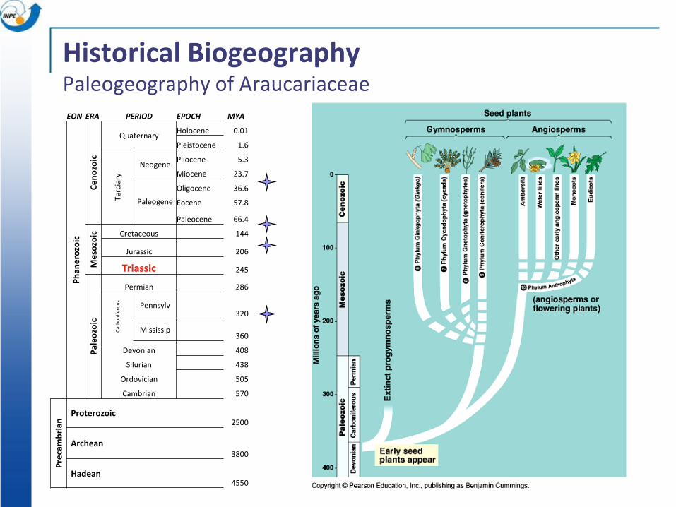
Historical Biogeography Paleogeography of Araucariaceae

EON ERA PERIOD EPOCH MYA

Ph

ane

rozo

ic

Ce

no

zoic

Quaternary Holocene 0.01

Pleistocene 1.6

Terc

iary

Neogene Pliocene 5.3

Miocene 23.7

Paleogene

Oligocene 36.6

Eocene 57.8

Paleocene 66.4

Me

sozo

ic

Cretaceous 144

Jurassic 206

Triassic 245

Pal

eo

zoic

Permian 286

Car

bo

nif

ero

us

Pennsylv 320

Mississip 360

Devonian 408

Silurian 438

Ordovician 505

Cambrian 570

Pre

cam

bri

an Proterozoic

2500

Archean 3800

Hadean 4550

Diorama of Araucariad Forest 200 million years ago

Diorama on display at the Rainbow Forest Museum, Petrified Forest National Park –

Arizona, USA.

http://www.scotese.com/climate.htm

Historical Climatic and Continental Changes

Barry Saltzman, Dynamical Paleoclimatology: Generalized Theory of Global Climate Change, Academic Press, New York, 2002

Historical Biogeography Paleogeography of Araucariaceae

Araucariaceae ancestors records

A. Upper triassic B. Jurassic C. Cretaceous (~ 210mya) (~ 180 mya) (~140 mya)

Fossil Cone

Araucaria mirabilis

(Patagonia ~165 mya)

Dutra & Stranz , 2004 www.scribd.com/doc/14112353/Dutra-Stranz-04

Historical Biogeography Paleogeography of Araucariaceae

Araucariaceae paleogeographic distribution

A. Cretaceous - Tertiary B. Eocene C. Oligocene – Miocene (~ 70 – 60 mya) (~ 55 mya) (~ 24 mya)

Dutra & Stranz , 2004 www.scribd.com/doc/14112353/Dutra-Stranz-04

Historical Biogeography

Distribution of extant species of the Genus

Araucaria De Jussieu

(Adapted from Kunzmann, 2007)

0º 0º

Total = 19 species – Oceania (17 sp) – South America (2 sp)

(19.000km2)

Araucaria Forest

Modern Biogeography Mixed Araucaria Forests –

exclusive of Southern Hemisphere

Two species in South America: Araucaria araucana (Chile)

Araucaria angustifolia (Brazil)

Life History & Structure Monodominance of long-lived

pioneers

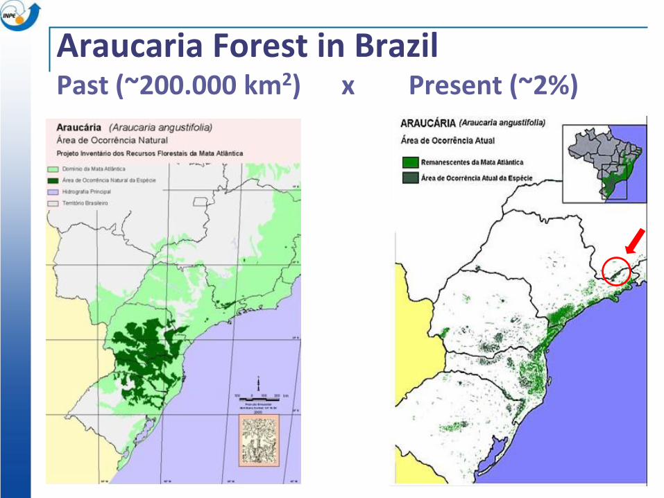
Araucaria Forest in Brazil Past (~200.000 km2) x Present (~2%)

Araucaria Forest Exploitation

Southern Brazil Inland Occupation 1895 – 1910 – Brazil Railway Co USA

Habitat loss – landcover conversion

Instituto de Pesquisa em Vida Selvagem e Meio Ambiente

Paraná

Araucaria Forest Exploitation

Instituto de Pesquisa em Vida Selvagem e Meio Ambiente

Paraná

ufrgs

Araucaria Forests Landscapes Southern Brazil

Lages -SC Guarapuava - PR

São Francisco de Paula - RS São José dos Ausentes - RS

Araucaria - PR

São Joaquim - SC

Araucaria Forests Landscapes Southeast Brazil

Tibor Jablonszky, 195?

Camanducaia

Campos do Jordão Campos do Jordão

São Bento do Sapucaí Cunha

Study Area Campos do Jordão State Park, SP

Forests and High Altitude Fields Mosaic (Campos do Jordão State Park - Ikonos Satellite Image – 2005)

Forests and High Altitude Fields Mosaic (Campos do Jordão State Park – 2008)

Forest Dynamics Data & Analysis

Methods:

1. Permanent plot (0.5ha)

2. Two inventories – 20 years apart (1988 – 2008)

3. Biometric and floristic data of all trees with dbh ≥ 1.6cm

4. All trees had their position recorded (x,y coordinates- 0.1m precision) and received an identification tag

Forest Dynamics Data & Analysis

Objective: to evaluate the forest dynamics

1.Mature forest or ongoing succession?

2.Which successional model better describes the forest dynamics?

Succession: “the non-seasonal, directional and continuous pattern of colonization and extinction on a site by species populations.” Begon et al., 1996

Primary Succession

Determinism

X

Stochasticity

Forest Dynamics Models

Succession: : “Succession refers to the changes observed in an ecological community following a perturbation that

opens up a relatively large space.” Connel & Slatyer, 1977

Secondary succession

Patch Dynamics Perspective

Disturbance

(gap, fire, landslide, storms, etc.)

Forest Dynamics Models

Dynamic Models for Ombrophyllous Mixed Forest

1. Biogeographical Model of Forest Expansion (Klein 1960)

2. Gap Model – Autogenic Succession (Jarenkow & Batista 1987)

3. Temporal Plot Replacement (Lozenge) (Ogden & Stewart 1995)

Biogeographical Model of Forest Expansion (Klein 1960)

Colonization of open areas

Monodominance of A. angustifolia

Understorey development

Developed forest

A. Angustifolia - emergent

Lauraceae & Myrtaceae - canopy

A. Angustifolia declines

Gap Model – Autogenic Succession (Jarenkow & Batista 1987)

Gap formation

Cicatrization

Structural regeneration

Temporal Stand Replacement “lozenge model”

(Ogden & Stewart 1995)

A – Recruitment

B – Thinning

C – Senescence

D – Second Cohort

DIS

TU

RB

AN

CE

Gap formation 1=2=3 = 50 years time span

Forest Dynamics Data & Analysis

Approaches:

1. Structural Dynamics – changes in basal area / height

2. Floristic Dynamics – changes in composition / diversity indexes

3. Dominant Population Dynamics - cover values

4. Horizontal Structural Dynamics (exploratory)

Methodology – Stand design / topography

1

5

1

5

5

9 13 5

9

40 plots – 12,5 x 10 m

trail

rivers

Results

1.Structural Dynamics – changes in basal area / height

2. Floristic Dynamics – changes in composition / diversity indexes

3. Dominant Population Dynamics - cover values

4. Horizontal Structural Dynamics (exploratory)

Whittaker Diagram

Results Dominant Populations

0

20

40

60

80

100

120

N_1988 N_2008 A_Basal 1988 A_Basal 2008

%

todos 14_selecionadas

83%

74%

90% 85%

Results Height stratification

1988 (t1) - 2008 (t2) Dominant tree populations (cover value)

(14 species)

emergents

canopy

understory

Results Diameter stratification

1988 (t1) - 2008 (t2) Dominant tree populations (cover value)

(14 species)

Emergents canopy understory

(exclusive)

12 24 36 48 60 72 84 96 108

X

0

8

16

24

32

40

48

56

64

72

Y

12 24 36 48 60 72 84 96 108

X

0

8

16

24

32

40

48

56

64

72

Y

12 24 36 48 60 72 84 96 108

X

0

8

16

24

32

40

48

56

64

72

Y

12 24 36 48 60 72 84 96 108

X

0

8

16

24

32

40

48

56

64

72

Y

12 24 36 48 60 72 84 96 108

X

0

8

16

24

32

40

48

56

64

72

Y

12 24 36 48 60 72 84 96 108

X

0

8

16

24

32

40

48

56

64

72

Y

1988 2008

Tree locations

All N= 2101 N=1741

dbh < 10 cm N= 1691 N=1336

dbh ≥ 10 cm N= 410 N=405

Tree Locations - Surface Density Maps Kernel Spatial Interpolation

5.74E-21

0.356

0.711

1.07

0 12 24 36 48 60 72 84 96 108

-12

0

12

24

36

48

60

72

84

5.74E-21

0.333

0.666

0.999

0 12 24 36 48 60 72 84 96 108

-12

0

12

24

36

48

60

72

84

7.09E-24

0.0826

0.165

0.248

0 12 24 36 48 60 72 84 96 108

-12

0

12

24

36

48

60

72

84

1.9E-21

0.366

0.733

1.1

0 12 24 36 48 60 72 84 96 108

-12

0

12

24

36

48

60

72

84

1.8E-22

0.329

0.659

0.988

0 12 24 36 48 60 72 84 96 108

-12

0

12

24

36

48

60

72

84

2.21E-21

0.0876

0.175

0.263

0 12 24 36 48 60 72 84 96 108

-12

0

12

24

36

48

60

72

84

1988 2008

All trees

dbh < 10 cm

dbh ≥ 10 cm

Mortality and Recruitment Surface Density Maps Kernel Spatial Interpolation

Chablis areas

= 1988 mapped logs;

= 2008 mapped logs

(darker’s over lighter’s).

A. angustifolia and P. lambertii - dap ≥ 50cm (stars)

Mortality Recruitment

Next Step

Goal:

To predict the effect of forest dynamics on

tree biomass, structure and species

composition

Next Step

Use of spatially explicit forest models

Steps: 1. Group species into functional types

2. Discriminate height groups

3. Parameterization of growth, mortality, recruitment rates

4. Characterize tree population structure (dbh) and

successional pattern

Plant Functional Types

Lavorel et al. Plant Functional Types: Are We Getting Any Closer to the Holy Grail? In: Canadell JG, Pataki D, Pitelka L (eds) (2007)

Terrestrial Ecosystems in a Changing World.

(i) bear some relationship to plant function

(ii) be relatively easy to observe and quick to quantify

(iii) using measurements that can be standardized across a wide range of species and growing conditions

(iv) have a consistent ranking – not necessarily constant absolute values – across species when environmental conditions vary

TROLL - Spatially Explicit Forest Model

1. “Competition for light is modelled by calculating exactly the three-dimensional field of photosynthetically active

radiation in the forest understorey.

2. Growth and mortality modules are similar to those of a classic gap model

3. Seed dispersal, dormancy and establishment success as well as a model of tree falls are also included.”

Chave, 1999.

Projeto FAPESP-PFMCG

Assessment of Impacts and Vulnerability to Climate Change

in Brazil and Strategies for Adaptation Options - IVA

Case Study 1: Studies on vulnerability to climate change and indicators of

vulnerability and impacts in the Paraiba do Sul Valley

(PP: Dr. Gilberto Fisch, IAE-CTA)

Araucaria Forest as vulnerability

indicator

Goals:

Modeling the potencial distribution of SE Brazil Araucaria Forests in different climate scenarios

Infer whether Dense Forest species will be favored at the expense of Araucaria Forests species

Forest x High Altitude Grassland

Mosaic

Vegetation Altitudinal Transect East of São Paulo State (Adapted from HuecK, 1972)

1. Ocean

2. Sand Beach

3. Dunes

4. Sandbank Forest

5. Mangrove

6. Rain Forest (coastal plain)

7. Rain Forest (lower slope)

8. Rain Forest (upper slope – mist)

9. Semideciduous Forest of South Paraiba Valley (gone)

10. Savanna (Cerrados)

11. Lowland Forest (floodplain)

12. High-altitude grasslands

13. Araucaria Forest

14. Podocarpus Forest (along the rivers)

OBRIGADA!

Nymphs Referata (to Miguel)

Nymphes et Satyre

William-Adolphe Bouguereau

(1825 - 1905)

La Nymphee