Embed Size (px)
Citation preview

LONG-TERM PERFORMANCE MODELLING OF ETOBICOKE EXFILTRATION
SYSTEM
By
Haiyue Liu
B.Eng, China University of Mining and Technology, 2013
A Thesis
Presented to Ryerson University
in partial fulfillment of the requirements for the degree of
Master of Applied Science
in the Program of
Civil Engineering
Toronto, Ontario, Canada, 2016
©Haiyue Liu 2016

ii
Author’s Declaration
I hereby declare that I am the sole author of this thesis. This is a true copy of the thesis, including
any required final revisions, as accepted by my examiners.
I authorize Ryerson University to lend this thesis to other institutions or individuals for the
purpose of scholarly research.
I further authorize Ryerson University to reproduce this thesis by photocopying or by other
means, in total or in part, at the request of other institutions or individuals for the purpose of
scholarly research.
I understand that my thesis may be made electronically available to the public.

iii
Abstract
Long-term Performance Modelling of Etobicoke Exfiltration System
Haiyue Liu
Master of Applied Science
Civil Engineering
Ryerson University
2016
Urbanization increases the stress on the hydrologic cycle. The Etobicoke exfiltration system
(EES) was developed in 1993 to remediate the impact on the hydrologic cycle after urbanization.
The purpose of this research is to model the Etobicoke exfiltration system (EES) and evaluate the
stormwater management performance of EES. A comprehensive literature review was conducted
on development of stormwater management and Low impact development (LID). The US EPA
SWMM was selected to model the EES. Three modelling methods were investigated to simulate
the performance of EES. The Orifice-Storage-Pump method was found to perform the best. EES
was applied before an existing wet pond in a case study subdivision. The modelling results show
that EES meets three criteria: reduce water quantity, impact water balance and improve water
quality.

iv
Acknowledgements
I would like to gratefully acknowledge my supervisor Dr. James Li for his guidance, support, and
inspiration throughout my master degree. My acknowledgement also extends to Dr. Darko
Joksimovic for his elaborative guidance in my modelling work. My last thanks go to Dr. Matyn
Hills for helping me proofread this thesis.

v
Dedication
To my parents for their support and love

vi
Table of Contents
Author’s Delaration ...................................................................................................................................... ii
Abstract ........................................................................................................................................................ iii
Acknowledgements ...................................................................................................................................... iv
Dedication ..................................................................................................................................................... v
Table of Contents ......................................................................................................................................... vi
List of Figures ............................................................................................................................................... x
Chapter 1 Introduction .................................................................................................................................. 1
1.1 Background ..................................................................................................................................... 1
1.2 Problem Identification..................................................................................................................... 4
1.3 Objective and Scope........................................................................................................................ 5
1.4 Organization of Thesis .................................................................................................................... 5
Chapter 2 Literature Review ......................................................................................................................... 7
2.1 Impacts of Urbanization .................................................................................................................. 7
2.1.1 Stormwater Quantity Impacts .............................................................................................. 7
2.1.2 Erosion Geomorphology Impacts ........................................................................................ 8
2.1.3 Stormwater Quality Impacts ................................................................................................ 9
2.1.4 Aquatic Habitat and Ecology ............................................................................................. 12
2.2 Evolution of Stormwater Management in Ontario ........................................................................ 12
2.3 Stormwater Management Criteria ................................................................................................. 14
2.4 Stormwater Management Facilities and Low Impact Development Practices.............................. 16
2.4.1 Introduction ........................................................................................................................ 16
2.4.2 Exfiltration Systems ........................................................................................................... 20
2.4.3 Wet Ponds .......................................................................................................................... 27
2.5 Best Management Practices .......................................................................................................... 28
2.6 Stormwater Management Models ................................................................................................. 28
Chapter 3 Modelling Approaches ............................................................................................................... 30
3.1 Etobicoke Exfiltration System (EES) ........................................................................................... 30

vii
3.1.1 The MIDUSS Modelling Approach ................................................................................... 33
3.1.2 Channel-Storage Modelling Approach .............................................................................. 34
3.1.3 Orifice-Storage Modelling Approach ................................................................................ 36
3.1.4 Orifice-Storage-Pump Modelling Approach ...................................................................... 39
3.2 Model Test Analysis ..................................................................................................................... 41
3.2.1 Model Test in MIDUSS ..................................................................................................... 41
3.2.2 Channel-Storage Method Test ........................................................................................... 42
3.2.3 Orifice-Storage Method Test ............................................................................................. 43
3.2.4 Orifice-Storage-Pump Method Test ................................................................................... 43
Chapter 4 Case Study .................................................................................................................................. 47
4.1 Site Description ............................................................................................................................. 47
4.2 Storm Sewer Network ................................................................................................................... 49
4.2.1 Subcatchment Parameters .................................................................................................. 49
4.2.2 Storm Sewer Design........................................................................................................... 51
4.2.2.1 Water Quantity ........................................................................................................ 51
4.2.2.2 Sewer Pipe Capacity ............................................................................................... 52
4.2.2.3 Junction Design ....................................................................................................... 53
4.2.3 Storm Sewer Network Sensitivity Analysis and Calibration ............................................. 53
4.3 Design of EES at the Case Study Area ......................................................................................... 55
4.3.1 Rainfall Data Analysis ....................................................................................................... 56
4.3.2 Temperature Data Analysis ................................................................................................ 59
4.4 EES-Wet Pond System Sensitivity Analysis................................................................................. 60
4.5 Summary of case study ................................................................................................................. 61
5.1 Stormwater Quantity ..................................................................................................................... 62
5.2 Water Balance ............................................................................................................................... 64
5.3 Stormwater Quality ....................................................................................................................... 67
Chapter 6 Conclusion and Recommendations ............................................................................................ 70
6.1 Conclusions ................................................................................................................................... 70
6.2 Recommendations ......................................................................................................................... 70

viii
References ................................................................................................................................................... 72
Appendix A – Subcatchment Parameters .................................................................................................... 76
Appendix B – Sewer Parameters ................................................................................................................ 77
Appendix C – Storage Parameters .............................................................................................................. 78
Appendix D - Junction Parameter Summary .............................................................................................. 79
Appendix E – Stormwater Quantity Model: Calibration Charts ................................................................. 80
Appendix F – Rainfall Data-By Descending Total Record Data ................................................................ 82
Appendix G – System Sensitivity Analysis – WetPond Head .................................................................... 84
Appendix H – System Sensitivity Analysis – Wet Pond Inflow and Outflow ............................................ 89

ix
List of Tables
Table 1 Comparisons of urban stormwater runoff concentrations with provincial water quality objectives
.................................................................................................................................................................... 10
Table 2 Suspended solids removed efficiency of different types of drainage area ..................................... 11
Table 3 Nutrient concentration and guidelines at the inlet of stormwater treatment facilities 12
Table 4 Guidelines and manuals corresponding to evolution of stormwater management......................... 14 Table 5 Water quality storage requirements based on receiving waters (Ministry of Environment (MOE),
2003) ........................................................................................................................................................... 15
Table 6 Pollutant removal efficiencies for soakaways, infiltration trenches and percentage of perforated
pipe systems (Credit Valley Conservation (CVC); Toronto and Region Conservation (TRCA), 2010) .... 21
Table 7 Trench parameters between MH2 and MH3 (Tran & Li, 2015) .................................................... 32
Table 8 Calibrated catchment parameters ................................................................................................... 33
Table 9 Calibrated trench parameters ......................................................................................................... 34
Table 10 Pipe parameters used in MIDUSS ............................................................................................... 34
Table 11 MH parameters used in SWMM .................................................................................................. 36
Table 12 Conduit parameters used in SWMM ............................................................................................ 36
Table 13 Orifice parameters used in SWMM ............................................................................................. 37
Table 14 Soil characteristics (Rossman, 2008) ........................................................................................... 49
Table 15 Pipe size and thickness (Ontario Concrete Pipe Association (OCPA), 1997) ............................. 53
Table 16 Trench design parameters ............................................................................................................ 56
Table 17 Selected gauge station information .............................................................................................. 57
Table 18 Selected gauge station information .............................................................................................. 59

x
List of Figures
Figure 1 Relationship between impervious cover and surface runoff (United States Environmental
Protection Agency, 2007) ............................................................................................................................. 7
Figure 2 Runoff hydrographs before and after development ........................................................................ 8
Figure 3 Cross-section of constructed EES ................................................................................................. 23
Figure 4 Typical profile of EES (A.M. Candaras Associates Inc., 1997) ................................................... 24
Figure 5 Rainfall hyetograph of October 5-6, 1995 historic event (A.M. Candaras Associates Inc., 1997)
.................................................................................................................................................................... 31
Figure 6 Measured trench hydraulics of EES for the Oct. 5-6, 1995 historic event ................................... 32
Figure 7 Representation of Channel-Dumbing Storage .............................................................................. 35
Figure 8 Representation of Orifice-Storage system in SWMM .................................................................. 37
Figure 9 Trench graphic model representations in SWMM ........................................................................ 38
Figure 10 Surface area-water depth in trench ............................................................................................. 39
Figure 11 Representation of Orifice-Storage-Pump System in SWMM ..................................................... 39
Figure 12 Pump curve in SWMM ............................................................................................................... 41
Figure 13 EES test results using MIDUSS ................................................................................................. 42
Figure 14 EES simulated results in SWMM for the Oct. 5-6, 1995 historic event. .................................... 44
Figure 15 EES head results using SWMM ................................................................................................. 45
Figure 16 EES MH2 Head results compared with measured MH2 Head .................................................... 45
Figure 17 MH3 Head results compared with measured MH3 Head ............................................................ 46
Figure 18 Map outlining the location of the subcatchment within the Town of Richmond Hill ................ 47
Figure 19 A satellite picture showing the terrain and drainage area of the subcatchment .......................... 48
Figure 20 Study area storm sewer network ................................................................................................. 50
Figure 21 Head difference - percent change in parameter .......................................................................... 54
Figure 22 Rainfall data analysis steps ......................................................................................................... 58
Figure 23 Rainfall data process steps .......................................................................................................... 59
Figure 24 Temperature record format ......................................................................................................... 60
Figure 25 Wet pond total inflow hydrograph 1 ........................................................................................... 63
Figure 26 Wet pond total inflow hydrograph 2 ........................................................................................... 63
Figure 27 Flow duration curve .................................................................................................................... 64
Figure 28 Predevelopment water balance ................................................................................................... 65
Figure 29 Wet pond without EES water balance ........................................................................................ 66
Figure 30 Wet pond with EES water balance ............................................................................................. 67
Figure 31 Wet pond without EES TSS reduction ....................................................................................... 68
Figure 32 Wet pond with EES TSS reduction ............................................................................................ 69
Figure 33 EES only TSS reduction ............................................................................................................. 69

1
Chapter 1 Introduction
1.1 Background
Urbanization has a drastic impact on the hydrologic cycle, especially on the natural process
of stormwater runoff. Compact urban development increases impervious areas inside a city,
which impacts the urban runoff in following ways: the runoff volume after development is
greater and the peak flow occurs sooner with higher magnitude and shorter duration. Urban
intensification also causes runoff related problems with regard to channel instability,
impaired habitat, losses of wetlands and so on. As a consequence, urbanization is recognized
as an important stressor to stream ecosystems.
According to the Ontario Ministry of Environment (MOE)’s Stormwater Management
Planning and Design Manual (2003), stormwater management facilities are categorized as lot
level controls, conveyance controls, and end-of-pipe controls. The term “treatment train” was
proposed to broader solutions to stormwater management by combining these three types of
facilities. By maintaining the natural hydrologic cycle, lot and conveyance controls can
reduce the size of end of pipe facilities, which are required for flood and erosion control.
(Ministry of Environment (MOE), 2003).
Traditional stormwater management has primarily dealt with water quantity and flood control.
However, over the past few years, stormwater management has been considering water
quality. As a consequence, Low Impact Development (LID) and Best Management Practices
(BMPs) have been developed accordingly.
According to Credit Valley Conservation (CVC), “Low impact development (LID) is a
stormwater management strategy that seeks to mitigate the impacts of increased runoff and

2
stormwater pollution by managing runoff as close to its source as possible”(Credit Valley
Conservation (CVC); Toronto and Region Conservation (TRCA), 2010). LID principles are
based on controlling stormwater at the source by the use of micro-scale controls that are
distributed throughout the site. The United States Environmental Protection Agency (US
EPA) defines LID as: "a set of site design strategies that minimize runoff and distributed,
small scale structural practices that mimic natural or predevelopment hydrology through the
processes of infiltration, evapotranspiration, harvesting, filtration and detention of water”
(United States Environmental Protection Agency, 2007). These practices can effectively
remove nutrients, pathogens and metals from surface runoff, as well as reduce stormwater
volume and intensity (Credit Valley Conservation (CVC); Toronto and Region Conservation
(TRCA), 2010).
The application of LID has both economical as well as environmental benefits. In 2007, the
US EPA investigated stormwater costs through 17 LID cases. The report indicates that
applying LID can reduce project costs and improve environmental performance (United
States Environmental Protection Agency, 2007). LID practices provide opportunities not only
to retrofit existing highly urbanized polluted areas but also to address environmental issues in
newly developed areas (United States Environmental Protection Agency (US EPA), 2000)
LID is currently one of the main tenets of Ontario Ministry of Environment and Climate
Change’s approaches to stormwater management. In 2015, a bulletin from the Ministry of
Environmental and Climate Changes (MOECC) suggested that the stormwater management
plans, which had been submitted to the ministry for Environmental Compliance Approval
(ECA), did not address preservation of the natural hydrology (Ministry of Environment and
Climate Change, 2015). Two steps were proposed to improve the implementation of LID:

3
“Clarify the ministry’s existing requirements and guidance on stormwater management” and
“Produce a LID stormwater management guidance document.”
Clearly, the principles for employing LID are outlined in MOECC’s related acts, regulations,
policies and guidelines. However, the guidance on LID can be improved in many respects
such as dealing with inconsistencies in the 2003 Stormwater Management Manual (Ministry
of Environment and Climate Change, 2015), and findings from this research can also serve to
supplement current LID practices, especially in relation to Etobicoke exfiltration system
(EES).
In a manner similar to the concept of LID, Water Sensitive Urban Design (WSUD) has been
proposed in Australia, which is an approach to urban planning and design that integrates the
management of the total water cycle into the urban development process (Government of
South Australia Adelaide, 2009). WSUD includes a pro-active process of recognizing the
design opportunities in order to intrinsically link landscape architecture and stormwater
management facilities (Wong, 2006). The innovation of stormwater management facilities
within an urban environment requires a shift to “at source” stormwater management systems.
Stormwater best management practices (BMPs) was proposed to control flood runoff events,
which uses a centralized location for stormwater management at the watershed level
(Dmodaram, Giacomoni, C. Prakash Khedun, Ryan, Saour, & Zechman, 2010). “Stormwater
Best Management Practices (BMPs) are techniques, measures or structural controls used to
manage the quantity and improve the quality of stormwater runoff” (United States
Environmental Protection Agency (US EPA), 1999). BMPs can be implemented to achieve a
variety of goals depending on the needs of practitioners. Three main goals should be

4
considered when applying BMPs: flow control, pollutant removal, and pollutant source
reductions (United States Environmental Protection Agency (US EPA), 1999).
1.2 Problem Identification
Although LIDs have been successful in pilot trials as an approach to stormwater management,
questions have been raised in regard to its suitability for all sites, groundwater contamination,
and winter performance (Dietz, 2007). For instance, there have been suggestions made that (1)
site conditions, such as soil permeability, slope, and water table depth, should be considered
when applying LID; and (2) community perception of LID may prevent its implementation
because homeowners want large lots and wide streets (United States Environmental
Protection Agency (US EPA), 2000). Moreover, several studies have shown the phosphorus
export from bio-retention systems could cause more harm to sensitive downstream water
bodies (Dietz, 2007). The total phosphorus export from bioretention systems in Canada has
been attributed to leaching of the mulch and organic soil media (Toronto and Region
Conservation, 2006). Additionally, Holman-Dodds et al. (2003) have shown that, in general,
LID technologies become less effective at higher rainfall.
The Etobicoke exfiltration system (EES) is one type of LID practices designed in 1993 to
address stormwater runoff volume over four seasons. During the 20 years’ development, EES
has been built and monitored in several places in Toronto (A.M. Candaras Associates Inc.,
1997)(Stormwater Assessment Monitoring and Perfomance Program, 2004). Although event
based performance of EES has already been investigated, there is a lack of research focusing
on the prediction of long-term performance of EES in terms of water quantity, water balance
and water quality.

5
1.3 Objective and Scope
This objective of this research thesis is to develop a modelling approach to predict the long-
term hydrologic performance of Etobicoke exfiltration system (EES). Using a development
site in the Town of Richmond Hill and the US EPA Storm Water Management Model
(SWMM), the hydrologic and water quality effect of EES were determined with and without
a downstream wet pond. The research focuses on the following investigations:
Apply the EES to a storm sewer network at the site and assess the performance of
EES in terms of stormwater runoff volume and peak flow reduction;
Assess the impact of the EES on wet pond total suspended solids (TSS) removal
efficiency;
Compare the pre-development and post-development (wet pond only; wet pond with
EES; EES only) water balance at the development site.
1.4 Organization of Thesis
This thesis consists of six chapters. Chapter 1 provides the background of this research,
problems definition as well as objective and scopes. Chapter 2reviews relevant literature,
including urbanization impacts, evolution of stormwater management in Ontario, stormwater
management criteria development, stormwater management facilities, low impact
development practices, best management practices, and stormwater management models.
Chapter 3 introduces the research methodology, including different methods of modelling
EES. Chapter 4 is the case study consisting of stormwater network in the study area, and
methods of data collection and application of the EES modelling methodology. Results of the

6
study are given in Chapter 5, while Chapter 6 provides a conclusion and makes
recommendations for future related research.

7
Chapter 2 Literature Review
2.1 Impacts of Urbanization
2.1.1 Stormwater Quantity Impacts
Urban development replaces vegetation with impervious surface such as roads, driveways,
parking areas, and building roofs, thus decreasing infiltration and evapotranspiration. As
shown in Figure1, the introduction of hard surfaces and reduction in vegetated cover impacts
the hydrologic circle (The Municipal Infrastructure Group Ltd.; Schollen & Company Inc.,
2011).
Figure 1 Relationship between impervious cover and surface runoff (United States
Environmental Protection Agency, 2007)

8
As such, urbanization will increase runoff rate and volume, as well as produce sooner peak
flow with higher magnitude and shorter duration as shown in Figure 2. At the same time, the
duration of a storm event is shorter after development. These higher peak flows, larger
volumes and higher velocity will increase the flood frequency and magnitude. Therefore, a
one-year storm peak flow will no longer occur once a year. For instance, at a watershed with
30% imperviousness, events which used to occur once a year (or two years) may occur 3.3
to 10.6 times a year (or two years)(Hollis, 1975).
Figure 2 Runoff hydrographs before and after development
(Source: http://www.civil.ryerson.ca/Stormwater/menu1/index.htm)
2.1.2 Erosion Geomorphology Impacts
The above hydrological alterations accelerate erosion resulting in unstable stream channels
and physical changes to accommodate higher flows (Bradford & Gharabaghi, 2004). The
larger amount of stormwater runoff caused by urbanization makes channels wider and
straighter from bank erosion (United States Environmental Protection Agency (US EPA),

9
1999). Additionally, because of in stream erosion and watershed inputs, sediment loads in
streams will increase and streambeds will be modified (Ministry of Environment (MOE),
2003).
2.1.3 Stormwater Quality Impacts
Urbanization has given rise to stormwater pollution problems since the latter part of the last
century. In a 1998 Report to Congress, the US EPA stated that urban stormwater runoff is the
fourth most extensive cause of water quality impairment of the nation’s rivers, and the third
most extensive source of water quality impairment of lakes (US EPA, 1990; Novotny &Olem,
1994). Pollution in runoff can come from both atmospheric and non-atmospheric sources
(Tsihrintzis & Hamid, 1997). The runoff stormwater picks up pesticides, road salts, heavy
metals, oils, bacteria, and other harmful pollutants and transports them through municipal
sewers into streams, rivers and lakes (Toronto and Region Conservation, 2012). Moreover,
biological communities are affected by hydrological alterations, stream form, temperature
regime, and water and sediment quality as well (Bradford & Gharabaghi, 2004). Table 1
shows a comparison of selected constituent concentrations and Ontario's Provincial Water
Quality Objectives (Ministry of Environment (MOE), 2003).
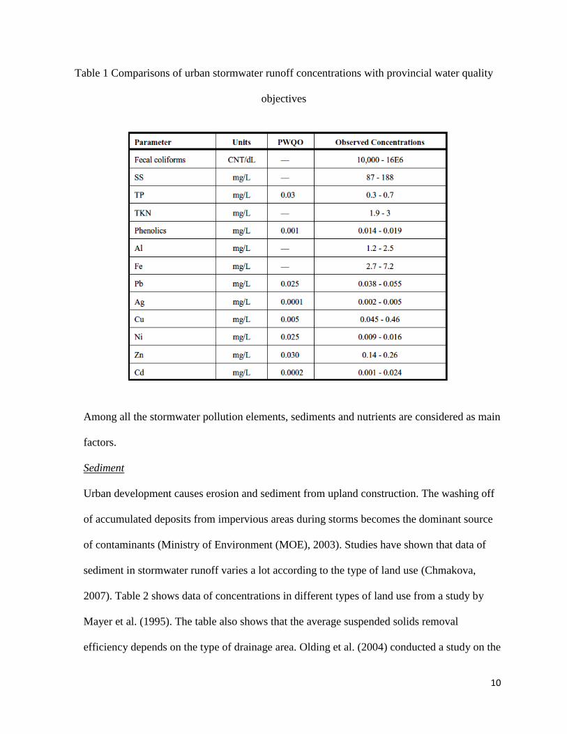
10
Table 1 Comparisons of urban stormwater runoff concentrations with provincial water quality
objectives
Among all the stormwater pollution elements, sediments and nutrients are considered as main
factors.
Sediment
Urban development causes erosion and sediment from upland construction. The washing off
of accumulated deposits from impervious areas during storms becomes the dominant source
of contaminants (Ministry of Environment (MOE), 2003). Studies have shown that data of
sediment in stormwater runoff varies a lot according to the type of land use (Chmakova,
2007). Table 2 shows data of concentrations in different types of land use from a study by
Mayer et al. (1995). The table also shows that the average suspended solids removal
efficiency depends on the type of drainage area. Olding et al. (2004) conducted a study on the

11
Richmond Hill ponds, showing that while TSS can be fairly high (around 908 mg/L), 75% of
TSS concentrations are below 60mg/L.
Table 2 Suspended solids removed efficiency of different types of drainage area
Type of land use
Concentration in
Stormwater runoff
(mg/L)
Removal efficiency
of ponds (%)
Residential area 5-267 24
Industrial area 8.8-119 25
Open area 0.5-66.8 0
Elevated levels of suspended solids, including organic and inorganic matter, have several
effects on water quality (Ministry of Environment (MOE), 2003):
Increased turbidity reduced light penetration;
Suspension clog gills and interfere with fish feeding;
Sediment covers spawning areas and smother benthic communities; and
Organic matter depresses the levels of dissolved oxygen.
Nutrients
Traditionally, nutrients are thought to be a major pollutant in agricultural runoff. However,
fertilizer application on lawns, golf courses and municipal recreation parks also cause
pollution. High concentrations of nutrients after urbanization can easily cause dissolved
oxygen depletion, ammonia and nitrate toxicity, and eutrophication. Several studies have
found nutrient concentration at the inlet of stormwater treatment facilities, as shown in Table
3. Although Mayer et al. (1995) contended that removal efficiency is very limited; other
studies have found that facilities with vegetation, especially macrophyte, could increase the
removal efficiency of nutrients (Groffman & Crawford, 2003).

12
Table 3 Nutrient concentration and guidelines at the inlet of stormwater treatment facilities
Type of nutrient Concentration so at the inlet of SWM
facilities Guidelines
Nitrate nitrogen 0.203-1.6mg/L (Mayer, Marsalek, & Reyes,
1995); 0.2-1.3mg/L (Mallin et al., 1992)
<10mg/L (Environmental
Canada, 1984)
Ammonia
nitrogen
0.013-1.082mg/L (Mayer, Marsalek, &
Reyes, 1995); 0.1-0.2mg/L (Stanley, 1996)
<0.5mg/L (Environmental
Canada, 1994)
Phosphate
phosphorus
0.007-0.48mg/L (Mayer, Marsalek, &
Reyes, 1995)
Excellent, if<0.1mg/L
(Center of Earth and
Environmental Science,
2005)
2.1.4 Aquatic Habitat and Ecology
Urbanization has negatively affected the aquatic habitat. Reduced baseflow, flow depth and
velocity, and poor water quality has impacted the aquatic habitat in the following ways:
Reduced the size of suitable aquatic habitat;
Influenced the aquatic species distribution within a stream;
Restricted fish spawning areas;
Decreased fish health, reproduction, feeding and diversity;
Decreased benthic macro invertebrates diversity; and
Caused excessive algae and eutrophication.
2.2 Evolution of Stormwater Management in Ontario
In order to reduce the impacts of urbanization, stormwater management was required to
manage runoff quantity and quality (The Municipal Infrastructure Group Ltd.; Schollen &
Company Inc., 2011). Stormwater management in Ontario originally focused on runoff
volume and peak flow control for the purpose of flood control, and only minor systems were

13
considered within stormwater management. However, after several years of development a
major system was introduced to reduce the size of the minor systems (Watt et al., 2003). In
the early 1990s, erosion and sediment loading as a result of urbanization became a concern.
Additionally, stormwater management was incorporated into urban development with respect
to land use and environmental effects (Ministry of Environment (MOE), 2003). By the end of
the 1990s, the Low Impact Development Stormwater Management Planning and Design
Guide proposed that stormwater management should focus on four aspects: water quality,
erosion control, aquatic habitat, and baseflow maintenance (Credit Valley Conservation
(CVC); Toronto and Region Conservation (TRCA), 2010). The Stormwater Management
Planning and Practices Manual (2003) proposed by Ontario's Ministry of Environment
introduced some current stormwater management technologies. In 2007, stormwater
management was required by the Environmental Bill of Rights to take account of the impacts
of climate change. Stormwater management developments in the past few years include not
only climate change, but also low impact development and water budget (Credit Valley
Conservation (CVC); Toronto and Region Conservation (TRCA), 2010). Table 4 indicates
guidelines and manuals corresponding to stormwater management evolution, which provide
the standards for stormwater management (Ternier, 2012). However, these guidelines restrict
opportunities to gain experience and become more innovative (Bradford & Gharabaghi,
2004).

14
Table 4 Guidelines and manuals corresponding to evolution of stormwater management
Authority Guidelines and Manuals
Ministry of Natural Resources, 1987 Guidelines on Erosion and Sediment Control
for Urban Construction Sites
Ministry of Environment and Ministry
of Natural Resources, 1991
Interim Stormwater Quality Control
Guidelines for New Development
Ministry of Environment and Ministry
of Natural Resources, 1993
Water Management on a Watershed Basis:
Implementing an Ecosystem Approach
Ministry of Environment and Ministry
of Natural Resources, 1993 Sub watershed planning
Ministry of Environment and Ministry
of Natural Resources, 1993
Integrating Water Management Objectives
into Municipal Planning Document
Ministry of Environment, 1994 1994 Stormwater Management Planning and
Practices Manual
Ministry of Environment, 2003 Stormwater Management Planning and
Practices Manual
2.3 Stormwater Management Criteria
With the development of stormwater management, design criteria have been developed to
consider interactions and cumulative effects (Ministry of Environment (MOE), 2003), and to
provide guidance on how to improve stormwater management practices (Bradford &
Gharabaghi, 2004). In 2003, Ontario's Ministry of Environment updated its 1994 version of
the Planning and Design Manual to include four main objectives of the stormwater
management design criteria: water quantity, water balance, water quality, and erosion control.
As runoff volume and peak flow increased with urban development, the criteria required that
the maximum peak flow should be within 2 to 100 years storms, which is the predevelopment
levels (Bradford & Gharabaghi, 2004). With regard to channel protection, geomorphic
thresholds for channel stability and requirements for habitat protection are taken into
consideration in the design criteria (Bradford & Gharabaghi, 2004). Although significant
improvements have been identified in the design criteria, refinements to channel protection

15
are still needed. The volumetric quality criteria are estimated using the SWMM model flow
prediction and a “Pond” sedimentation model (Bradford & Gharabaghi, 2004). There are
three levels of pond water quality protection: enhanced protection, normal protection, and
basic protection. Table 5 presents the volumetric water quality criteria (Ministry of
Environment (MOE), 2003). The criteria also take nutrients, bacteria and temperature into
consideration. Ontario's Ministry of Environment uses this model to determine groundwater
recharge as well. However, as some data cannot support this model's approach, calculating an
annual recharge volume requirement is used instead (Bradford & Gharabaghi, 2004).
Table 5 Water quality storage requirements based on receiving waters (Ministry of Environment
(MOE), 2003)

16
2.4 Stormwater Management Facilities and Low Impact Development Practices
2.4.1 Introduction
LID is the current evolution in stormwater management (The Municipal Infrastructure Group
Ltd.; Schollen & Company Inc., 2011). The main objectives of LID practices are to:
maximize infiltration, maximize evapotranspiration, maximize reuse and minimize hard
surfaces.
In this section, several stormwater management facilities and LID practices are introduced.
Green roofs
“Green roofs", also known as “living roofs” or “rooftop gardens”, consist of a thin layer of
vegetation and growing medium installed on top of a conventional flat or sloped roof (Credit
Valley Conservation (CVC); Toronto and Region Conservation (TRCA), 2010). Green roofs
can benefit cities as they improve energy efficiency, reduce urban heat island effects, and
create green space for passive recreation or aesthetic enjoyment. There are two types of green
roofs, one type is intensive green roof with a 15cm depth of growing medium and the other is
extensive green roof with a 15cm or less depth of growing medium. The construction of
green roofs should take structural requirements, roof slope and drainage area and runoff
volume into consideration (Credit Valley Conservation (CVC); Toronto and Region
Conservation (TRCA), 2010). Green roofs are especially effective in older urban areas with
chronic combined sewer overflow (CSO) problems, due to the high level of imperviousness
(United States Environmental Protection Agency (US EPA), 2000). Applying extensive
green roofs in Europe has extended the life of roofs, reduced energy costs and conserved
valuable land. Research in Germany showed that the 3 inch design offers the highest benefit
to cost ratio (United States Environmental Protection Agency (US EPA), 2000).
17
Grass swales
“Enhanced grass swales are vegetated open channels designed to convey, treat and attenuate
stormwater runoff (are also referred to as enhanced vegetated swales)” (Credit Valley
Conservation (CVC); Toronto and Region Conservation (TRCA), 2010). Grass swales or
channels are often located adjacent to roads and sidewalks, are adaptable to a variety of site
conditions, are flexible in design and layout, and are relatively inexpensive (US Department
of Transportation). Grass swales can be used to reduce runoff velocity by holding the water
until it infiltrates the soil, or directs it to another infiltrating area. Sedimentation, infiltration
and adsorption works together to reduce water pollutants. During construction, decreasing
the slope or providing dense cover should be considered to reduce the erosion of soils
(United States Environmental Protection Agency (US EPA), 2000).
Permeable pavements
“Permeable pavements, also known as porous pavement, an alternative to traditional
impervious pavement, allow stormwater to drain through them and into a stone reservoir
where it is infiltrated into the underlying native soil or temporarily detained” (Credit Valley
Conservation (CVC); Toronto and Region Conservation (TRCA), 2010). The system can be
categorized as full infiltration, partial infiltration, and partial infiltration with flow restrictor.
Porous pavements are best suited for low traffic areas, such as parking lots and sidewalks.
The most successful installations of alternative pavements are found in coastal areas with
sandy soils and flatter slopes (Center for Watershed Protection, 1998). At the end of the
twentieth century the cost of paving blocks and stones in Maryland, USA, ranged from US$2
to US$4, whereas asphalt cost US$0.50 to US$1 (Center for Watershed Protection, 1998).
Infiltration trenches

18
Infiltration trenches, also known as infiltration galleries or linear soakaways, refer to
infiltration systems with a subsurface storage component that treat stormwater runoff from
several lots as opposed to soakaways pits that are primarily used for a single lot application.
“Infiltration trenches are rectangular trenches lined with geotextile fabric and filled with
clean granular stone or other void forming material” (Credit Valley Conservation (CVC);
Toronto and Region Conservation (TRCA), 2010). Infiltration trenches can hold water in the
spaces between stones and excess water soaking into the ground will flow to another
overflow area or system, and they can be implemented at the ground surface to intercept
overland flows, or underground as part of a storm sewer system (Ministry of Environment
(MOE), 2003). The acceptability of infiltration trenches should be confirmed because of
potential concerns for aquifer contamination. In most cases, infiltration trenches will provide
marginal flooding and erosion control benefits because they are sized for recharge and water
quality (Ministry of Environment (MOE), 2003).
Bio-retention systems
Bio-retention systems consist of a topping layer of hard wood mulch, a vegetative layer and a
porous media layer. The depression area can hold water with the plants and shrubs growing
to increase water tolerance. Water flows into the bio-retention area by means of swales, curb
openings or pipes. Accordingly, the bio-retention system are categorized as without an
underdrain for full infiltration, with an underdrain for partial infiltration, or with an
impermeable liner and underdrain for filtration only, which can also be referred to as a bio-
filter (Credit Valley Conservation (CVC); Toronto and Region Conservation (TRCA), 2010).
Bio-retention systems perform well for the attenuation of stormwater runoff, as well as in
removal of pollutants. Microbes presenting in the bio-retention system break down organic

19
compounds, which are then killed by the pathogens exposed to sunlight. The pollutants are
removed by infiltrating stormwater through the riparian buffers. The suspended solid (SS)
will settle at the bottom of the bio-retention system where the stormwater enters into the bio-
retention system. Vegetation aids in sedimentation by removing TSS, litter, and debris and
nutrients attached to the sediment particles (United States Environmental Protection Agency
(US EPA), 2000). The application of fertilizer in watershed or directly used in the bio-
retention cell will introduce the presence of nutrients, such as phosphate and nitrate. There
are experiments showing that phosphate existing in stormwater perform the function of
removing metal in the bio-retention system due to the potential of phosphate of immobilizing
divalent heavy metals from wastewater, solid waste, and contaminated soils (Ma et al., 2002).
Other sources estimated the costs for developing bio-retention sites at between US$3 and
US$15 per square foot of bio-retention area (US EPA, 2000). According to design guidelines,
bio-retention systems occupy 5-7% of the drainage system and have many economic benefits.
At the same time, storm sewers can be reduced with a bio-retention system. For example,
bio-retention practices reduced the amount of storm drain pipes at a medical office building
in Prince George's County, Maryland, USA, from 800 to 230 feet, which resulted in a cost
savings of US$24,000 or 50% of the overall drainage cost for the site (Department of
Environmental Resources, 1993). Maintenance of bio-retention systems is required annually
including plant material, soil layer and mulch layer. Plants will provide enhanced
environmental benefits over time as root systems and leaf canopies increase in size and
pollutant uptake and removal efficiencies (United States Environmental Protection Agency
(US EPA), 2000). Soil will lose the ability of filtering pollutant over time (United States
Environmental Protection Agency (US EPA), 2000).

20
Combined LID practices
Damodaram et al. (2010) conducted research to simulate the combined BMPs and LID
practices using combination systems of rain harvesting system and permeable pavements,
which perform better at reducing peak flow than the single rain harvesting system or
permeable pavements scenarios. Villarreal et al. (2004) presented an overview of a new open
stormwater system of BMPs in series ranging from green-roofs to stormwater ponds and
open channels installed in the inner city suburb of Augustenborg in Malmo, southern Sweden.
Investigation of the water balance from 2001 to 2002 found that green-roofs had the effect of
reducing total runoff and that the ponds successfully attenuate storm peak flows for even a
10-year rainfall. Brown et al. (2012) compared the performance of pervious concrete with
subsurface storage in series with bio-retention system (PC-B) with individual LID practices
(bioretention). The results showed that hydrologic performance was significantly improved.
The PC-B system had treated additional 10% of annual runoff volume, discharged about half
as much outflow volume, and lowered peak outflow rates (Brown, 2012). However as to the
water quality, only TSS and TAN (Total ammoniacal nitrogen) concentrations were
significantly reduced (Brown, Line, & Hunt, 2012). The city of Portland in Oregon, USA,
has a Green Streets program that combines rain gardens and permeable pavements, green
roofs and sidewalks swales. The city estimates to reduce the peak flows by as much as 85%,
stormwater volume by 60%, and water pollution by up to 90% (Pazwash, 2011).
2.4.2 Exfiltration Systems
In this research, an Etobicoke exfiltration system is used as a LID to improve the
effectiveness of a wet pond. Exfiltration systems are also known as perforated pipe systems,
pervious pipe systems, clean water collector systems, and percolation drainage systems.

21
Exfiltration Systems can be used in place of conventional storm sewer pipes, where
topography, water table depth, and runoff quality conditions are suitable (Credit Valley
Conservation (CVC); Toronto and Region Conservation (TRCA), 2010). Several studies of
exfiltration systems in Ontario have examined their water quality benefits, as shown in Table
6 below.
Table 6 Pollutant removal efficiencies for soakaways, infiltration trenches and percentage of
perforated pipe systems (Credit Valley Conservation (CVC); Toronto and Region Conservation
(TRCA), 2010)
Etobicoke exfiltration system was first developed and constructed in 1993 by the City of
Etobicoke in the Greater Toronto Area (GTA), Ontario. The main objective of EES is to
retrofit the conventional storm sewer system without end-of-pipe treatment for stormwater
quality control. In addition, EES is one of the solutions in response to the new direction set
by the Province of Ontario Interim Stormwater Quality Control Guidelines for New
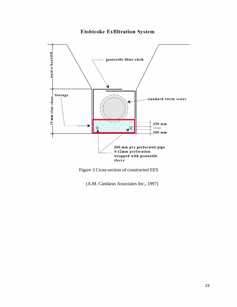
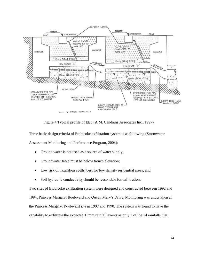
Development (MOEE and MNR, 1991). As indicated in Figure 3 and 4, two perforated pipes
are installed below the main stormwater sewer. Runoff from catch basin enters the main

22
stormwater sewer. With the level of stormwater in the manhole increases, stormwater runs
into the perforated pipes first and then exfiltrates into the gravel trench. The whole
exfiltration system is embedded in a gravel-filled trench, which is designed to meet
stormwater requirements and is separated from the local soils with a geotextile fabric. The
two perforated pipes have the same slope as the storm sewers and are wrapped by the filter
cloth to prevent the pollutant from entering the trench. A goss trap is designed to trap the
pollutants in the high traffic areas as well as the old municipality areas, where floatables and
spills occur frequently. In order to prevent the soil and water in the trench from migrating to
the downstream trench, the cut-off walls are added in the EES. A mechanical plug is
designed to be installed at each downstream manhole; however, during construction this plug
is located in the upstream to protect the perforated pipes from being clogged by the
construction material.
Benefits of EES include that it can be used throughout the year and achieve the objective of
controlling runoff intensity, volume, quality, duration and frequency (Ternier, 2012).
Compared to other infiltration facilities, EES is intended to eliminate the need to reconstruct
and replace the filtration medium (A.M. Candaras Associates Inc., 1997).
23
Figure 3 Cross-section of constructed EES
(A.M. Candaras Associates Inc., 1997)
24
Figure 4 Typical profile of EES (A.M. Candaras Associates Inc., 1997)
Three basic design criteria of Etobicoke exfiltration system is as following (Stormwater
Assessment Monitoring and Perfomance Program, 2004):
Ground water is not used as a source of water supply;
Groundwater table must be below trench elevation;
Low risk of hazardous spills, best for low density residential areas; and
Soil hydraulic conductivity should be reasonable for exfiltration.
Two sites of Etobicoke exfiltration system were designed and constructed between 1992 and
1994, Princess Margaret Boulevard and Queen Mary’s Drive. Monitoring was undertaken at
the Princess Margaret Boulevard site in 1997 and 1998. The system was found to have the
capability to exfiltrate the expected 15mm rainfall events as only 3 of the 14 rainfalls that

25
exceeded 15mm caused overflows. The EES is sensitive to the rate of runoff and antecedent
conditions and the limitation parameter is the throughout capacity.
Analysis of a limited set of sediment samples indicated that heavy metal concentrations were
generally higher than those of stormwater retention pond sediments (A.M. Candaras
Associates Inc., 1997). The water quality data was limited for monitoring because of a lack
of measurable flow data and the small numbers of overflow events.
Furthermore, EES can be designed to handle the runoff from extreme summer, winter and
early spring events (Ternier, 2012). Ontario’s four distinct seasons, fall, winter, spring and
summer, each have their unique climate and rainfall patterns in regard to precipitation
volume, intensity, frequency, duration, and direction (Singh, 1997). Cao et al. (2009) found
that summer (mid June to August) had most of the severe rainfall events. Dichkinson (2010)
supported the results by showing that in Southern Ontario, the return period for an event with
a specific rainfall volume and duration decreased in summer compared with spring or fall.
High intensity and short duration storm events in early fall (September and October) is
similar to summer; however, as temperature falls in November, the rainfall events tend to be
of medium intensity and long duration.
Winter (December to mid March) and spring (mid March to mid June) in Ontario is generally
in the form of low intensity and long duration events (MOE, 2003). There are few runoff
problems in winter as the cold weather keeps the snow with a frost layer on the top of the soil.
However, once melting begins, the runoff needs taking care of (Ternier, 2012). Vink and
Chin (2004) analyzed flow data from 1955 to 1997 for four streams in the GTA and found
that spring had the highest peak mean daily flows. There are three different methods of
snowmelt: pavement melt, road melt, and pervious area melt. The last two methods occur

26
periodically during the winter and lead to large peak flows with rain or snow events at the
end of winter (Roseen, et al., 2009). Snow can accumulate pollutants from the air as well as
contaminants from the ground and the soluble pollutants will percolate downwards and
accumulate at the bottom with snow pack melting (Oberts, 2000). Due to the below freezing
temperatures that are typical of winters in Ontario and similar cold climate countries,
infiltration and filtration stormwater management practices have been viewed with hesitation
(Roseen, et al., 2009).
Many northern cold climate countries have focused on stormwater management based on
cold climates and Ontario is no exception (Ternier, 2012). Most of the stormwater
infrastructures are designed based on rainfall from summer and fall, without considering rain
on snow events. Rain-on-snow events bring many problems such as resulting erosion as well
as accumulation of pollutants like suspended solids and heavy metal. Existing stormwater
management facilities have few methods for dealing with these problems. MOE SWM
Planning and Design (2003) shows that infiltration trenches and bioretention systems are
inappropriate for water quality treatment during winter and spring due to limited capacity
from freezing or soil saturation. Although several recent sources assert that bioretention
systems function in cold climate as frozen media has minimal effect on hydraulic function,
more investigations need to be done (Roseen R. , et al., 2009)(Davidson, LeFevre, & Oberts,
2008)Wet ponds are recommended for water quality control during winter and spring.
However, ponds may easily become stratified during hot summers with 3m or greater depth
(Ministry of Environment (MOE), 2003).

27
2.4.3 Wet Ponds
End-of-pipe stormwater management facilities include wet ponds, wetlands, dry ponds and
infiltration basins (Ministry of Environment (MOE), 2003). The difference between wet
ponds and wetlands is the proportions of deep (>0.5m) and shallow (<0.5m) areas. The deep
zones of wet ponds take around 80% surface of the facilities.
Virtually all the new wet facilities designed in Ontario have an extended detention storage
component in need of multi-purpose design, which is used during and after a runoff event.
(Ministry of Environment (MOE), 2003)
During the last 10 to 15 years, wet ponds have become an increasingly popular best
management practice in Ontario. Binstock (2011) indicated that stormwater management in
Ontario has primarily used conveyance and end-of-pipe controls, with the main choice being
detention ponds among all the variety of stormwater facilities.
The performance of a wet pond is time dependent and steadily decreases as sediment
accumulation occurs.Thus maintenance becomes necessary for wet ponds to keep meeting
the regulation for discharged water quality. There are several factors impacting the
maintenance of wet ponds, such as storage volume, rainfall intensity and duration,
construction activities, street sweeping, and characteristics of the pond drainage area
(Ministry of Environment (MOE), 2003).The literatures describe annual maintenance costs as
a percentage of construction costs or a function of the pond’s design storage volume, or as a
function of the subcatchment area.

28
2.5 Best Management Practices
In response to the detrimental ecological stresses that urbanization places on a watershed,
best management practices (BMPs) have been developed to reduce water quantity impacts
and water quality constituents (Khowaja, 2007). BMPs can be either non-structural or
structural. Non-structural BMPs include institutional, educational or pollution prevention
practices designed to prevent pollutants from entering stormwater runoff or reduce the
volume of stormwater requiring management (United States Environmental Protection
Agency (US EPA), 1999). Infiltration systems, detention systems, retention systems etc. are
structural BMPs designed to protect wetlands and ecosystems, improve water quality, protect
water resources, and control floods (United States Environmental Protection Agency (US
EPA), 1999). Some BMPs may enhance recharge, which is often considered a secondary
management benefit (Newcomer, Gurdak, Sklar, & Nanus, 2014). However, BMPs have
little effect on inadequate base flow, flashy hydrology and other hydrologic development
impact (Coffman, 2000; (United States Environmental Protection Agency (US EPA), 2000).
Site suitability has a significant effect on the performance of BMPs strategies; therefore,
several factors such as drainage areas, land uses, average rainfall frequency, duration and
intensity, and soil types should be taken into consideration.
2.6 Stormwater Management Models
Water resource computer models are very important tools for evaluating pre- and post-
development conditions (Toronto and Region Conservation, 2012). Several models are
recommended within TRCA’s jurisdiction for the purpose of analyzing hydrology, hydraulics
and water balance. Stormwater Hydrology models are categorized as single event and

29
continuous simulation. Event based modelling is used to input individual events for
establishing flow rates and for designing peak reduction and attenuation facilities (Toronto
and Region Conservation, 2012). In contrast, a continuous model can be used to input long-
term precipitation events for long term simulation as well as evaluation of erosion potential
(Toronto and Region Conservation, 2012). MIDUSS is one of the event based stormwater
models with an EES modelling option (Richard, 2013). Ternier (2012) calibrated an EES
using MIDUSS to analyze its effectiveness under various synthetic storm events.
The EPA Storm Water Management Model (SWMM) is a dynamic rainfall-runoff simulation
model used for single or long-term (continuous) simulation of runoff quantity and quality
from primarily urban areas (Rossman, 2008). Thousands of studies have already been
conducted to simulate non-point pollution sources and the transport of pollutants (Rossman,
2008). Some of the studies used SWMM to simulate LID and consequently discovered some
of SWMM's deficiencies. McCutcheon and Wride (2013) found that in SWMM there were
differences between LID parameters for single event and long-term parameters, that moisture
conditions before a storm may influence LID infiltration capacity, that during short-term
storms it is easier to compensate for clogging or debris, and that gaps existed between their
field observations and model results.

30
Chapter 3 Modelling Approaches
3.1 Etobicoke Exfiltration System (EES)
The area selected for the investigation of modelling approaches for EES is located at the
Princess Margaret Boulevard. This site (one of the three demonstration sites) was monitored
by the Stormwater Assessment Monitoring and Performance Program’s staff (SWAMP) from
1996 to 1998 (SWAMP 2004). Various modelling approaches were conducted on the first
upstream section of EES (between MH2 and MH3) because of the available monitored data.
The soil type of this area is silty sandy to clayed silt (A.M. Candaras Associates Inc., 1997).
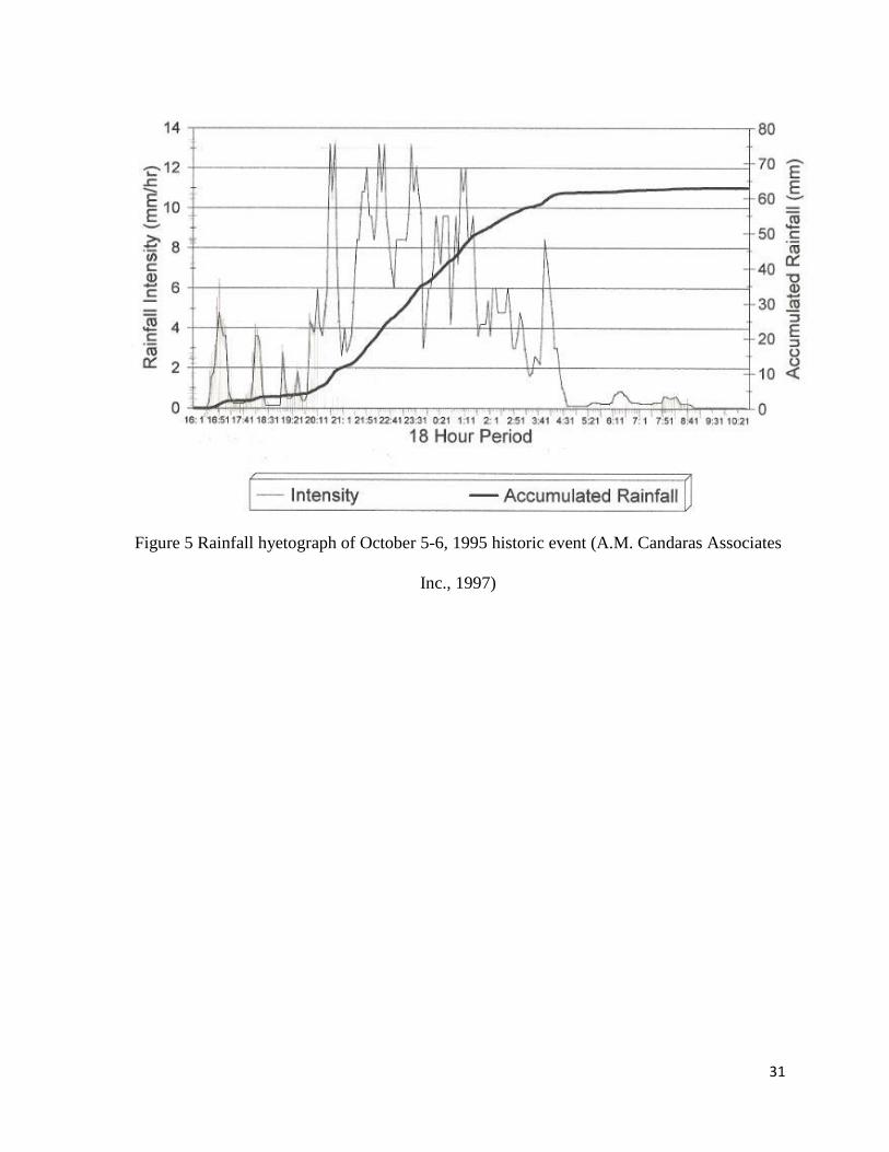
The storm event, “October 5-6, 1995”, monitored at Toronto Lester B. Pearson International
Airport rainfall station with Climate ID 6158733, was used as rainfall input to calibrate EES
using various modelling approaches. The storm duration was 18 hours with 63mm of rainfall,
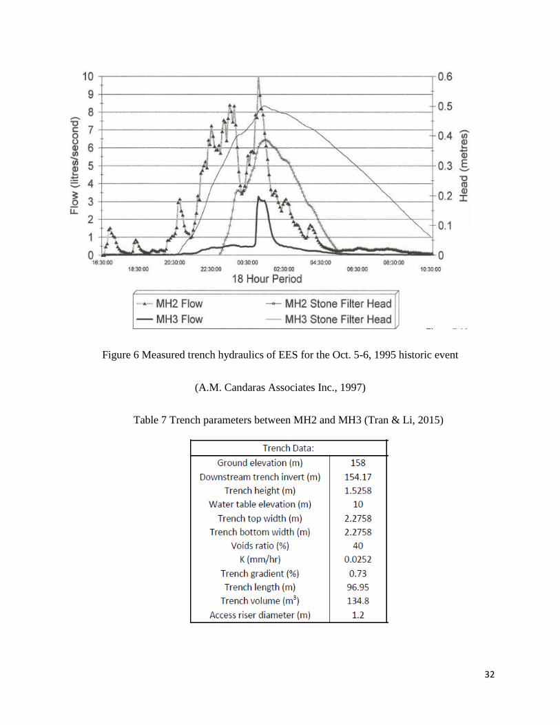
as shown in Figure 5. The measured trench hydraulics (i.e. flows and heads) of the EES for
the event on October 5-6th, 1995 is shown in Figure 6.The trench data are listed in Table 7.
31
Figure 5 Rainfall hyetograph of October 5-6, 1995 historic event (A.M. Candaras Associates
Inc., 1997)
32
Figure 6 Measured trench hydraulics of EES for the Oct. 5-6, 1995 historic event
(A.M. Candaras Associates Inc., 1997)
Table 7 Trench parameters between MH2 and MH3 (Tran & Li, 2015)

33
3.1.1 The MIDUSS Modelling Approach
MIDUSS has a modelling option of perforated pipes underneath a storm sewer and is used by
Ternier (2012) to model EES. In this study, the monitored rainfall data in Figure 5 were input
into MIDUSS, and then catchment and trench parameters were calibrated with the measured
trench hydraulics as shown in Table 8 and 9.
Table 8 Calibrated catchment parameters

34
Table 9 Calibrated trench parameters
Storm sewer pipes and perforated pipes could be modelled by MIDUSS with the parameters
as shown in Table 10. Pipe 1 was the traditional storm sewer pipe and Pipe 2 and Pipe 3 were
perforated pipes.
Table 10 Pipe parameters used in MIDUSS
MIDUSS was calibrated to match the measure overflow along the storm sewer. Since
MIDUSS is an event-based simulation model, it could not be used to simulate long-term
runoff control performance.
3.1.2 Channel-Storage Modelling Approach
Although SWMM has a variety of options to model different LID practices (e.g. Bio-
Retention Cell, Rain Garden, Green Roof, Infiltration Trench, Permeable Pavement, Rain
Barrel and Vegetative Swale), it does not have a modelling option for EES. As a result,
several different modelling approaches are proposed in this study to model EES using
35
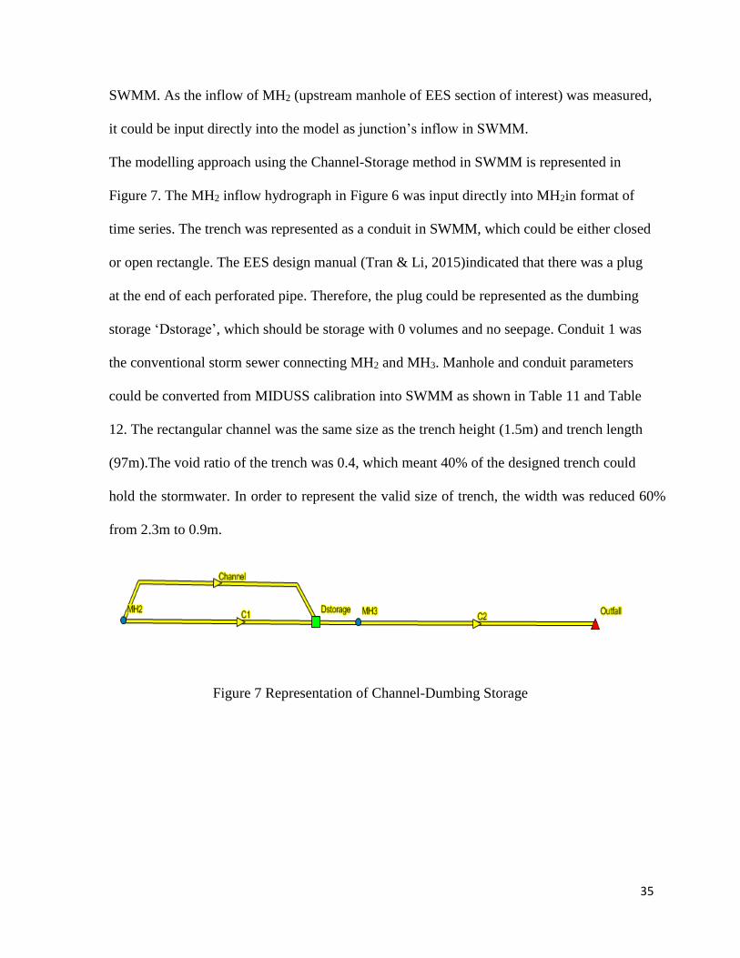
SWMM. As the inflow of MH2 (upstream manhole of EES section of interest) was measured,
it could be input directly into the model as junction’s inflow in SWMM.
The modelling approach using the Channel-Storage method in SWMM is represented in
Figure 7. The MH2 inflow hydrograph in Figure 6 was input directly into MH2in format of
time series. The trench was represented as a conduit in SWMM, which could be either closed
or open rectangle. The EES design manual (Tran & Li, 2015)indicated that there was a plug
at the end of each perforated pipe. Therefore, the plug could be represented as the dumbing
storage ‘Dstorage’, which should be storage with 0 volumes and no seepage. Conduit 1 was
the conventional storm sewer connecting MH2 and MH3. Manhole and conduit parameters
could be converted from MIDUSS calibration into SWMM as shown in Table 11 and Table
12. The rectangular channel was the same size as the trench height (1.5m) and trench length
(97m).The void ratio of the trench was 0.4, which meant 40% of the designed trench could
hold the stormwater. In order to represent the valid size of trench, the width was reduced 60%
from 2.3m to 0.9m.
Figure 7 Representation of Channel-Dumbing Storage

36
Table 11 MH parameters used in SWMM
MH parameters
Name MH2 MH3
Invert Elev(m) 154.877 154.17
Depth(m) 3.123 3.83
Table 12 Conduit parameters used in SWMM
Conduit parameters
Name C1 C2
Length(m) 96.95 96.95
Roughness 0.013 0.013
Inlet Offset(m) 0.709 0.709
Outlet Offset(m) 0.709 0.709
Cross-Section CIRCULAR CIRCULAR
Geom1(m) 0.45 0.45
Since SWMM Version 5.1 includes a new “Seepage Rate (mm/hr)” function of conduits, it
was used to model EES. If the Seepage Rate is the rate of water flowing out from
perforations along a conduit; it should be equal to the soil conductivity. The Seepage Rate of
conduit was changed within a reasonable soil conductivity range of 20-70mm/hr to test
whether it could simulate the exfiltrating rate of the perforated pipes.
3.1.3 Orifice-Storage Modelling Approach
A representation of the Orifice-Storage method in SWMM is shown in Figure 8. In this
method, manholes and conduits were set up same as Channel-storage method. However,
trench was represented by storage instead of channel. Two orifices represented the inlet of
the perforated pipes, so the inlet offset was 0.3m. The height of the orifice was 0.2m, which
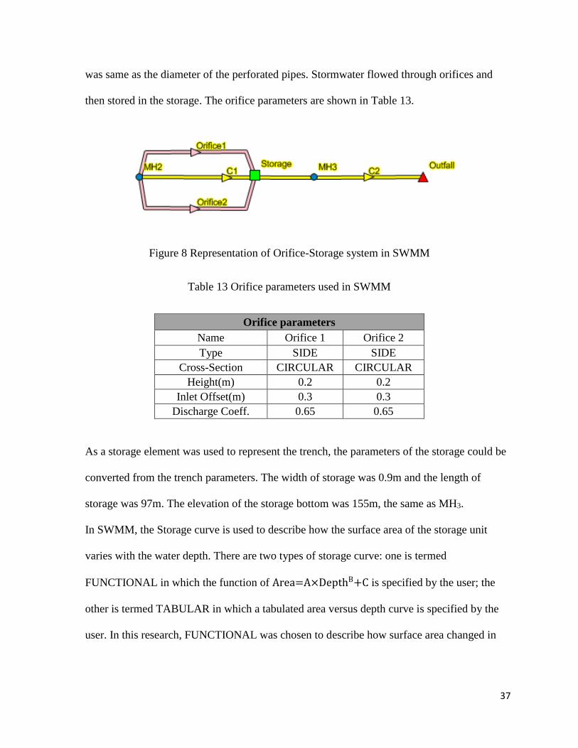
37
was same as the diameter of the perforated pipes. Stormwater flowed through orifices and
then stored in the storage. The orifice parameters are shown in Table 13.
Figure 8 Representation of Orifice-Storage system in SWMM
Table 13 Orifice parameters used in SWMM
Orifice parameters
Name Orifice 1 Orifice 2
Type SIDE SIDE
Cross-Section CIRCULAR CIRCULAR
Height(m) 0.2 0.2
Inlet Offset(m) 0.3 0.3
Discharge Coeff. 0.65 0.65
As a storage element was used to represent the trench, the parameters of the storage could be
converted from the trench parameters. The width of storage was 0.9m and the length of
storage was 97m. The elevation of the storage bottom was 155m, the same as MH3.
In SWMM, the Storage curve is used to describe how the surface area of the storage unit
varies with the water depth. There are two types of storage curve: one is termed
FUNCTIONAL in which the function of Area=A×DepthB+C is specified by the user; the
other is termed TABULAR in which a tabulated area versus depth curve is specified by the
user. In this research, FUNCTIONAL was chosen to describe how surface area changed in
38
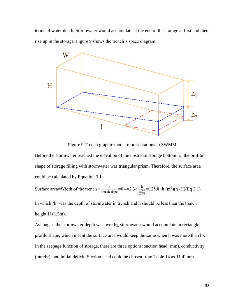
terms of water depth. Stormwater would accumulate at the end of the storage at first and then
rise up in the storage. Figure 9 shows the trench’s space diagram.
Figure 9 Trench graphic model representations in SWMM
Before the stormwater reached the elevation of the upstream storage bottom h2, the profile’s
shape of storage filling with stormwater was triangular prism. Therefore, the surface area
could be calculated by Equation 3.1.
Surface area=Width of the trench ×h
trench slope=0.4×2.3×
h0.709
96.95
=125.8×h (m2)(h<H)(Eq 3.1)
In which ‘h’ was the depth of stormwater in trench and h should be less than the trench
height H (1.5m).
As long as the stormwater depth was over h2, stormwater would accumulate in rectangle
profile shape, which meant the surface area would keep the same when h was more than h2.
In the seepage function of storage, there are three options: suction head (mm), conductivity
(mm/hr), and initial deficit. Suction head could be chosen from Table 14 as 11.42mm
39
initially. Conductivity was assumed to be the calibrated value from MIDUSS 27mm/hr.
Initial deficit was 0 for constant seepage rate equal to conductivity.
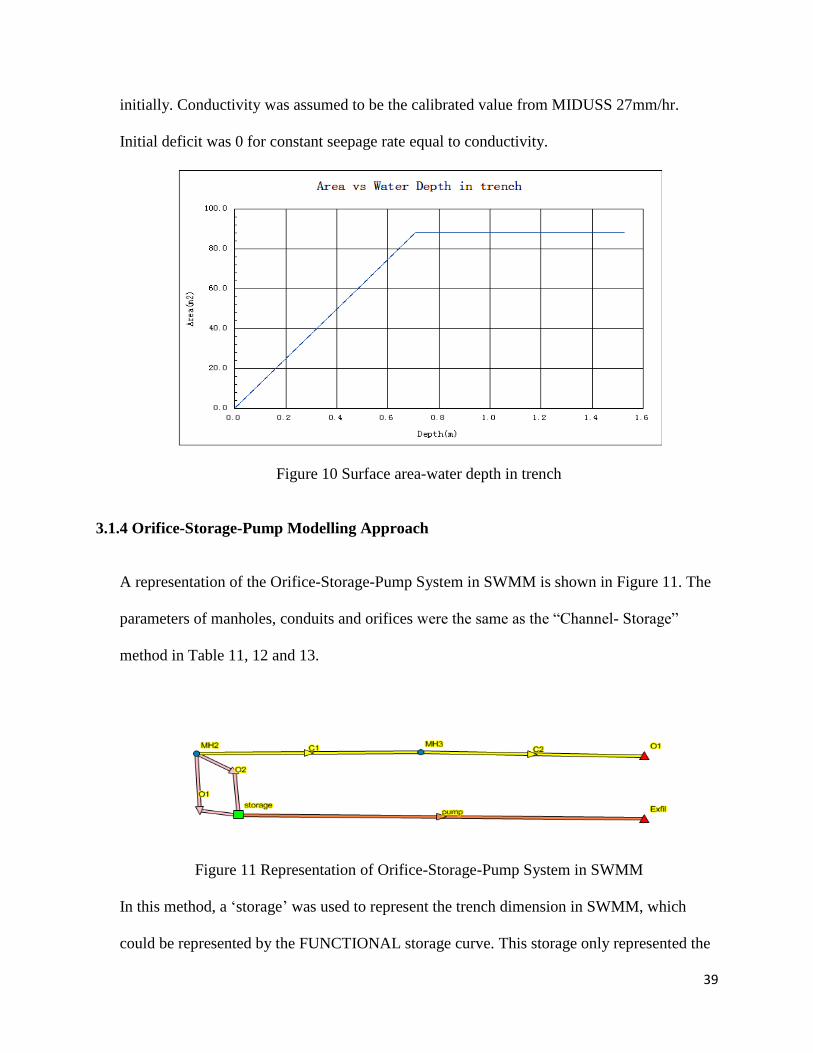
Figure 10 Surface area-water depth in trench
3.1.4 Orifice-Storage-Pump Modelling Approach
A representation of the Orifice-Storage-Pump System in SWMM is shown in Figure 11. The
parameters of manholes, conduits and orifices were the same as the “Channel- Storage”
method in Table 11, 12 and 13.
Figure 11 Representation of Orifice-Storage-Pump System in SWMM
In this method, a ‘storage’ was used to represent the trench dimension in SWMM, which
could be represented by the FUNCTIONAL storage curve. This storage only represented the

40
dimension of the trench holding stormwater; therefore, the storage wouldn’t take trench slope
and exfiltration rate into consideration. Thus, the Coefficient A and B were both assumed to
be 0 in SWMM. The value of Coefficient C for the functional curve of the storage was set as
the effective area of trench surface, which should be 88m2 (0.9m×97m) because of the 40%
void rate. As this method didn’t take trench slope into consideration, the elevation of the
storage should be set same as the upstream elevation of the trench, which was the elevation
of upstream MH2.
In order to model the trench slope and exfiltration rate, a pump was added to the storage. The
pump curve represented the exfiltration rate of water flowing from both bottom and sides of
the trench to surrounding soil. Therefore, the outflow from the perforated pipes Qoutflow(in
terms of soil conductivity k for the pump curve) could be calculated by Equation 3.2, in
which W was the width of the trench and L was the length of the trench. After the water
depth h in the trench was over trench height (1.5m), Q would become constant as shown in
Figure 12.The designed value for the soil conductivity k was set according to calibrated
hydraulic conductivity in MIDUSS.
Qoutflow(L/s) =k(
mm
hr)
3600(s/hr)×1000(mm
m)
×Wetted area (m2) × 1000 (L/m3)
= (k/3600 × (W × 0.4 + 2 × h) × L(L
S) (Eq 3.2)

41
Figure 12 Pump curve in SWMM
3.2 Model Test Analysis
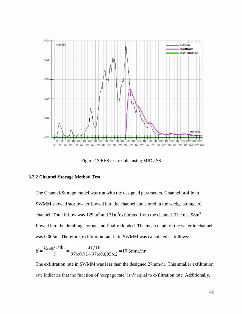
3.2.1 Model Test in MIDUSS
The modelling results of EES using MIDUSS show good agreement with the monitored
overflow volume of 42.2 m3and trench hydraulics, as shown in Figure 13. Peak flow reduced
from 0.01m3/s to 0.005 m3/s. The calibrated hydraulic conductivity k was 27mm/hr. Since
MIDUSS is an event-based model, it cannot be used to simulate long-term performance of
EES.
42
Figure 13 EES test results using MIDUSS
3.2.2 Channel-Storage Method Test
The Channel-Storage model was run with the designed parameters. Channel profile in
SWMM showed stormwater flowed into the channel and stored in the wedge storage of
channel. Total inflow was 129 m3 and 31m3exfiltrated from the channel. The rest 98m3
flowed into the dumbing storage and finally flooded. The mean depth of the water in channel
was 0.005m. Therefore, exfiltration rate k’ in SWMM was calculated as follows:
k'=Qexfil/18hr
S=
31/18
97×0.91+97×0.005×2=19.3mm/hr
The exfiltration rate in SWMM was less than the designed 27mm/hr. This smaller exfiltration
rate indicates that the function of ‘seepage rate’ isn’t equal to exfiltration rate. Additionally,

43
the stormwater wouldn’t stop flowing into the trench and accumulate in the MH2 when the
water level was higher than the elevation of the orifices. As a result, no flow was detected in
Conduit 1.
3.2.3 Orifice-Storage Method Test
The Orifice-Storage model was run with the designed parameters. From the Candara’s’
report (1997), 4m3of stormwater exfiltrated from storage and the rest 97m3of stormwater was
stored in the wedge storage of trench. However, the continuity error was -11%.
The mean depth of the water in storage was 1m. Therefore, exfiltration rate could be
calculated below but did not match the designed 27mm/hr. This calculated exfiltration rate
indicates SWMM won’t exfiltrate the stormwater stored in trench. So in order to add the
exfiltration rate into the model, a pump is added in the following method.
K'=Qexfil/18hr
S=
4/18
97×0.91+97×1×2=0.7mm/hr
3.2.4 Orifice-Storage-Pump Method Test
The Orifice-Storage-Pump model was run with the designed parameters. After calibrating the
k value to 32 mm/hr, the simulated outflow hydrograph was found to be in good agreement
with to the measured data.
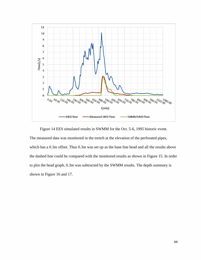
As can be seen from the flow curves in Figure 14, the inflow of MH2 is input data. After
calibration, the peak flow in MH3was 3L/s, which was in good agreement with those
observed. The minor flow of the observed MH3 flow was interpreted in Post-Construction
Evaluation of EES as minor leakage through the connected catchbasins and the water
entering through an abandoned culvert connection (A.M. Candaras Associates Inc., 1997).
44
Figure 14 EES simulated results in SWMM for the Oct. 5-6, 1995 historic event.
The measured data was monitored in the trench at the elevation of the perforated pipes,
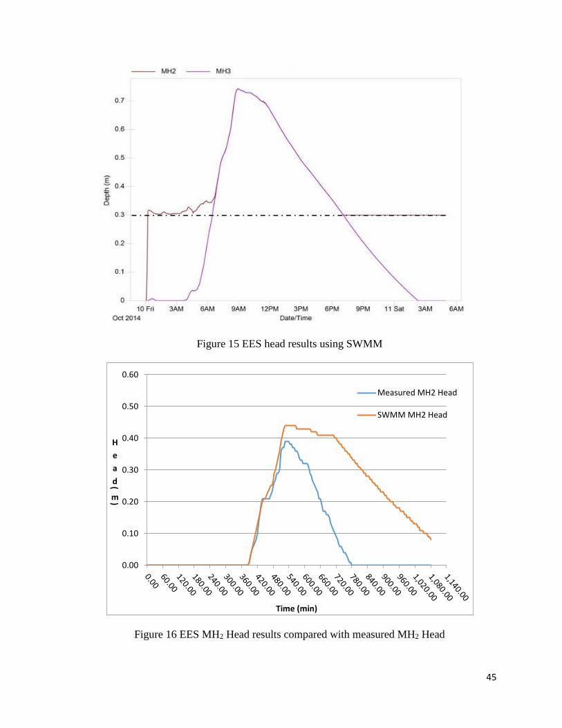
which has a 0.3m offset. Thus 0.3m was set up as the base line head and all the results above
the dashed line could be compared with the monitored results as shown in Figure 15. In order
to plot the head graph, 0.3m was subtracted by the SWMM results. The depth summary is
shown in Figure 16 and 17.
45
Figure 15 EES head results using SWMM
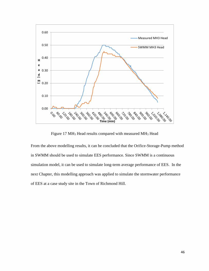
Figure 16 EES MH2 Head results compared with measured MH2 Head
0.00
0.10
0.20
0.30
0.40
0.50
0.60
H
e
a
d(
m)
Time (min)
Measured MH2 Head
SWMM MH2 Head
46
Figure 17 MH3 Head results compared with measured MH3 Head
From the above modelling results, it can be concluded that the Orifice-Storage-Pump method
in SWMM should be used to simulate EES performance. Since SWMM is a continuous
simulation model, it can be used to simulate long-term average performance of EES. In the
next Chapter, this modelling approach was applied to simulate the stormwater performance
of EES at a case study site in the Town of Richmond Hill.
0.00
0.10
0.20
0.30
0.40
0.50
0.60
H
e
a
d(
m)
Time (min)
Measured MH3 Head
SWMM MH3 Head

47
Chapter 4 Case Study
4.1 Site Description
According to Toronto and Region Conservation Authority for the Living City, the watershed
of GTA is divided into 8 regions (Humber River, Rouge River, Etobicoke & Mimico Creek,
Duffins& Carruthers Creeds, Highland Creek, Don River, Petticoat Creek, and Lake Ontario
Water front watershed). The selected site for this research is located at the south-east of
Bayview Avenue and Elgin Mills Road, in the Town of Richmond Hill within the Rouge
River region as shown in Figures 18 and 19.
Figure 18 Map outlining the location of the subcatchment within the Town of Richmond Hill

48
Figure 19 A satellite picture showing the terrain and drainage area of the subcatchment
There are two main zones within the Rouge River considering the contiguous and uniform
climate: the Lake Ontario shore zone and the South Slope. The selected area is in the range of
the South Slope zone, with relatively higher topography and less influence from Lake
Ontario. The mean annual temperature of the portion of the South Slope zone is
approximately 7°C (Sanderson, 2004). During summer, high air temperatures usually reach
the mid to upper 20°C but several special days reach the low and mid 30°C. However, winter
temperatures vary a lot from daytime to midnight. An incursion of warm air from the south
that pushes a January day up over 10°C can easily be followed by an Arctic air mass and
overnight lows below -25°C (Toronto and Region Conservation, 2007). Thus, the stormwater
management design in this area should consider the variation of temperatures during winter.
The selected site, which is in the Peel Plain region, consists of sandy loam and other fine-
particle fraction and is relatively flat. According to the soil condition, soil characteristics can
be chosen from Table 14. The site is relatively flat with a 2% slope. Following the existing
site grade, the stormwater runoff flows to the southeast of the site where the pond is located.
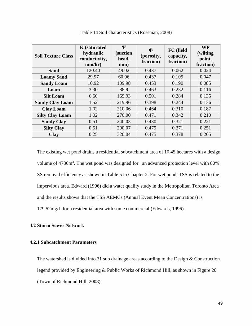
49
Table 14 Soil characteristics (Rossman, 2008)
Soil Texture Class
K (saturated
hydraulic
conductivity,
mm/hr)
Ψ
(suction
head,
mm)
Φ
(porosity,
fraction)
FC (field
capacity,
fraction)
WP
(wilting
point,
fraction)
Sand 120.40 49.02 0.437 0.062 0.024
Loamy Sand 29.97 60.96 0.437 0.105 0.047
Sandy Loam 10.92 109.98 0.453 0.190 0.085
Loam 3.30 88.9 0.463 0.232 0.116
Silt Loam 6.60 169.93 0.501 0.284 0.135
Sandy Clay Loam 1.52 219.96 0.398 0.244 0.136
Clay Loam 1.02 210.06 0.464 0.310 0.187
Silty Clay Loam 1.02 270.00 0.471 0.342 0.210
Sandy Clay 0.51 240.03 0.430 0.321 0.221
Silty Clay 0.51 290.07 0.479 0.371 0.251
Clay 0.25 320.04 0.475 0.378 0.265
The existing wet pond drains a residential subcatchment area of 10.45 hectares with a design
volume of 4786m3. The wet pond was designed for an advanced protection level with 80%
SS removal efficiency as shown in Table 5 in Chapter 2. For wet pond, TSS is related to the
impervious area. Edward (1996) did a water quality study in the Metropolitan Toronto Area
and the results shows that the TSS AEMCs (Annual Event Mean Concentrations) is
179.52mg/L for a residential area with some commercial (Edwards, 1996).
4.2 Storm Sewer Network
4.2.1 Subcatchment Parameters
The watershed is divided into 31 sub drainage areas according to the Design & Construction
legend provided by Engineering & Public Works of Richmond Hill, as shown in Figure 20.
(Town of Richmond Hill, 2008)
50
Figure 20 Study area storm sewer network
The area of each subcatchment and curb length could be measured in Google Earth. % Zero
Imperv’ in SWMM represents the percent of impervious area with no depression storage
including roads, sidewalks and driveways. ‘%Imperv’ in SWMM is defined by all
impervious surfaces including roofs as downspouts have been disconnected from the storm
sewers. By measuring area of impervious area with no depression storage and impervious
surfaces, ‘%Zero’ and ‘%Imperv’ were calculated.
The width of subcatchment could be calculated using the following equation after measuring
longest flow length of each area:
Width(m) =Area of Subcatchment (ha)×10000
longest flow length (m) (Eq 4.1)
As the primary soil type within the drainage area is sandy loam, suction head, conductivity
and initial deficit parameters can be obtained from soil characteristics given in Table 14.
Depth of depression storage on impervious and pervious area, can be retrieved from the

51
Richard’s wet pond model (Richard, 2013). Parameters of subcatchments are displayed in
Appendix A.
4.2.2 Storm Sewer Design
The storm sewer was designed in accordance with the Richmond Hill Standards and
Specifications Manual.
4.2.2.1 Water Quantity
Runoff peak flow is estimated using the Rational Formula:
Qq =Air
360 (Eq 4.2)
Where,
Qq = the runoff quantity, m3/s;
A =drainage area, ha;
i = average rainfall intensity, mm/hr;
r = runoff coefficient.
The drainage area is obtained in the previous step. The land use type of this area is single
family residential, so the runoff coefficient is 0.45(Town of Richmond Hill, 1998). The 5-yr
rainfall intensity is calculated as follows:
i = 991 × (T + 4)^(−0.808) (Eq 4.3)
Where,
T =time of concentration, (min).

52
4.2.2.2 Sewer Pipe Capacity
The capacity of storm sewers is computed using the Manning equation:
Q =1×R
23×S
12×A
n (Eq 4.4)
And
V =1×R
23×S
12
n (Eq 4.5)
Where,
Q = flow, m3/s;
A = nominal cross-section area of the sewer, m2;
R = hydraulic radius, m;
S = slope of sewer, m/m;
n = roughness coefficient, for concrete pipe, n = 0.013;
v = velocity, m/s.
Hydraulic radius can be calculated using the following equation, in which Pw (m) and Aw (m2)
are the wetted perimeter and area of the pipe:
R =Pw
Aw (Eq 4.6)
Slope of the sewer is based on the topography of the area. For concrete pipes, the roughness
coefficient is assumed to be 0.013. The size of pipes should be adapted until the velocity is in
the range of 0.85-5m/s. According to the Concrete Pipe Design Manual, the pipe size could
be chosen from Table 15. Also the minimum size for sewer mains should range from 0.3m to

53
0.9m. The size of sewers can be altered until the pipe capacity is larger than the peak runoff.
The parameters of sewers are shown in Appendix B.
Table 15 Pipe size and thickness (Ontario Concrete Pipe Association (OCPA), 1997)
Pipe size (m), d 0.3 0.375 0.45 0.525 0.6 0.675 0.75 0.825
Thickness (mm), a 44 47 57 69 94 100 107 113
4.2.2.3 Junction Design
The inlet elevation of the wet pond was determined to be 213.5m from Richard’s wet pond
model (Richard, 2013). The last sewer of the sewer system C29 has a downstream elevation
(213.5m); therefore Equation 4.7 is used to calculate the upstream junction elevation. In this
way, all the junctions’ elevations could be calculated.
Upstream elevation = Downstream elevation + Slope ∗ Length of Pipe (Eq 4.7)
The sewers’ inlet elevation should be 0.85m (0.2m+0.35m+0.3m) higher than the junction’s
bottom elevation. Trench elevation was assumed to be the junction elevation.
Junction depth is difference between Junction bottom and Junction ground elevation. The
ground elevations are determined from the 1-meter elevation contour lines for the Regional
Municipality of York (Open Data, 2011).
4.2.3 Storm Sewer Network Sensitivity Analysis and Calibration
The August 24-27, 2007 rainfall event was chosen for sensitivity analysis. Sensitivity
analysis (i.e. the percent change of the pond head) was performed using nine parameters in
the storm sewer network system. Although the model parameters are typically tested within a
range of ±25% of the designed values (James, 2005), this study used a range of ±50% for the
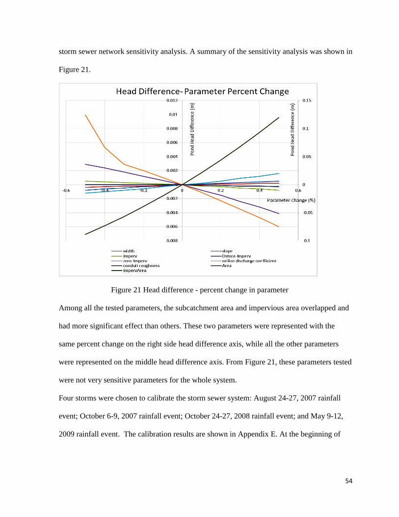
54
storm sewer network sensitivity analysis. A summary of the sensitivity analysis was shown in
Figure 21.
Figure 21 Head difference - percent change in parameter
Among all the tested parameters, the subcatchment area and impervious area overlapped and
had more significant effect than others. These two parameters were represented with the
same percent change on the right side head difference axis, while all the other parameters
were represented on the middle head difference axis. From Figure 21, these parameters tested
were not very sensitive parameters for the whole system.
Four storms were chosen to calibrate the storm sewer system: August 24-27, 2007 rainfall
event; October 6-9, 2007 rainfall event; October 24-27, 2008 rainfall event; and May 9-12,
2009 rainfall event. The calibration results are shown in Appendix E. At the beginning of

55
these four 3-day events, wet pond head was about 213.45m. After the simulation, the wet
pond head ended around 213.5m after 3 days.
4.3 Design of EES at the Case Study Area
Using the Planning and Design Manual of the Etobicoke Exfiltration System for Stormwater
Management (Tran & Li, 2015), the EES was designed at the case study site. EES should not
be applied in the first and the last trenches of the storm sewer network. Every sewer trench is
different because the storm sewer size increases from upstream to downstream end of the
network. Trench design of the trench effective dimension and exfiltration rate is described
below.
Effective Trench Dimension
Trench gradient was assumed to be the same as that of the storm sewer. Trench length was
equal to the length of storm sewer. Trench height and width were calculated using Equation
4.8 and 4.9 based on the Candara’s (1997) cross-section diagram (Figure 3) and City of
Etobicoke Works Department (City of Etobicoke, 1992).
Trench Height = 0.3 + 0.35 + 2 ∗ a + d + 0.3 = (d + 2a + 1.15)m (Eq 4.8)
Trench Width = 2 ∗ [0.5m +0.2
2m + 0.25m] + dm + 2 ∗ a m = (d + 2a + 1.7)m (Eq 4.9)
In which ‘a’ (mm) is the thickness of concrete pipes add’ (m) is the diameter of the pipes.
Thickness of concrete pipes could be determined from Table 16 (Ontario Concrete Pipe
Association (OCPA), 1997). However, the thickness of perforated pipes could be neglected
because of the relatively small sizes.

56
Table 16 Trench design parameters
Height above concrete pipe 0.3m
Perforated pipe diameter 0.2m
Distance between inverts of concrete pipe and perforate pipe 0.35m
Depth below perforated pipe 0.3m
Distance between trench boundary and middle of perforated pipe 0.5m
Distance between closest edges of perforated pipe and concrete pipe 0.25m
Storage area was related to the depth of trench given by Area=A×DepthB+C. Coefficient A
and B were both given as 0 in SWMM. The C value of the storage was the effective area of
the trench:
C = 40% ∗ W ∗ L (Eq 4.10)
Where,
W = width of the trench, m;
L = length of the trench, m.
Parameters of storage are shown in Appendix C.
Exfiltration rate (Pump curve)
As the soil type was sandy loam, the hydraulic conductivity was 10.4mm/hr as shown in
Table 14. The exfiltration rate was calculated using Equation 3.2.
In the following analysis, the PCSWMM commercial software based on SWMM model) was
used. The EES was modelled using Orifice-Storage-Pump method.
4.3.1 Rainfall Data Analysis
Rainfall data was based on a rainfall station with comprehensive records located close to the
study area. The original data was processed to generate continuous rainfall data for the
project. Climatic data were sourced from the National Archive System, Meteorological

57
Service of Canada. Among the 271 gauge stations with hourly precipitation and temperature
records in Ontario, 7 stations have records of more than 45 years of selected gauge station
information (Table 17). TONRONTO gauge and TORONTO LESTER B. PERSON INT’L
A gauge was nearer to the study area compared with other gauges. Although TORONTO
gauge station had 65 years’ rainfall data recorded, however, the mean observation on count
of this gauge was less than TORONTO LESTER B. PERSON INT’L A. Therefore, in order
to include more valid values, rainfall and temperature data were collected from TORONTO
LESTER B. PERSON INT’L A gauge station with Climate ID 6158733 from 1960 to 2013.
Table 17 Selected gauge station information
Location Name Climate
ID
Year
Count
Earlies
t Year
Most
Recent
Year
Mean
Obser
vation
Count
Distance
From
Study
Area (km)
HLY
03 SAULT STE MARIE A 6057592 47 1961 2007 6084 493.78
HLY
03
KINGSTON PUMPING
STATION 6104175 47 1960 2007 5677 237.37
HLY
03 WINDSOR A 6139525 48 1960 2007 7418 340.36
HLY
03
FERGUS SHAND
DAM 6142400 48 1960 2007 5316 76.67
HLY
03 TORONTO 6158350 65 1937 2002 6266 24.41
HLY
03
TORONTO LESTER B.
PEARSON INT'L A 6158733 54 1960 2013 7227 29.61
HLY
03 TRENTON A 6158875 50 1964 2014 6836 152.35
The record rainfall data had some un-valued data such as M-99999, M000000, and -99999 as
well as some missing data. In order to select continuous rainfall days with the least missing
or un-valued data, the rainfall data were processed by following the steps in Figure 22. After
counting the number of Valued days and Non-Valued days in each year, the years were
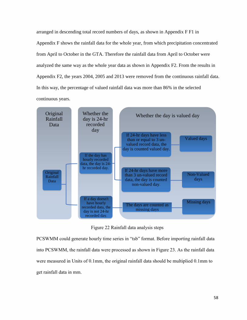
58
arranged in descending total record numbers of days, as shown in Appendix F F1 in
Appendix F shows the rainfall data for the whole year, from which precipitation concentrated
from April to October in the GTA. Therefore the rainfall data from April to October were
analyzed the same way as the whole year data as shown in Appendix F2. From the results in
Appendix F2, the years 2004, 2005 and 2013 were removed from the continuous rainfall data.
In this way, the percentage of valued rainfall data was more than 86% in the selected
continuous years.
Figure 22 Rainfall data analysis steps
PCSWMM could generate hourly time series in “tsb” format. Before importing rainfall data
into PCSWMM, the rainfall data were processed as shown in Figure 23. As the rainfall data
were measured in Units of 0.1mm, the original rainfall data should be multiplied 0.1mm to
get rainfall data in mm.
Whether the day is valued day Whether the day is 24-hr
recorded day
Original Rainfall
Data
Original Rainfall
Data
If the day has hourly recorded
data, the day is 24-hr recorded day.
If 24-hr days have less than or equal to 3 un-
valued record data, the day is counted valued day.
Valued days
If 24-hr days have more than 3 un-valued record data, the day is counted
non-valued day.
Non-Valued days
If a day doesn't have hourly
recorded data, the day is not 24-hr recorded day.
The days are counted as missing days
Missing days
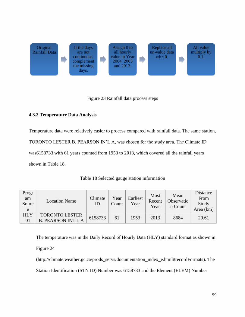
59
Figure 23 Rainfall data process steps
4.3.2 Temperature Data Analysis
Temperature data were relatively easier to process compared with rainfall data. The same station,
TORONTO LESTER B. PEARSON IN’L A, was chosen for the study area. The Climate ID
was6158733 with 61 years counted from 1953 to 2013, which covered all the rainfall years
shown in Table 18.
Table 18 Selected gauge station information
Progr
am
Sourc
e
Location Name Climate
ID
Year
Count
Earliest
Year
Most
Recent
Year
Mean
Observatio
n Count
Distance
From
Study
Area (km)
HLY
01
TORONTO LESTER
B. PEARSON INT'L A 6158733 61 1953 2013 8684 29.61
The temperature was in the Daily Record of Hourly Data (HLY) standard format as shown in
Figure 24
(http://climate.weather.gc.ca/prods_servs/documentation_index_e.html#recordFormats). The
Station Identification (STN ID) Number was 6158733 and the Element (ELEM) Number
Original Rainfall Data
If the days are not
continuous, complement the missing
days.
Assign 0 to all hourly
value in Year 2004, 2005 and 2013.
Replace all un-value data
with 0.
All value multiply by
0.1.

60
was78. The Value was 24-hour record temperature data and the Flag should be in
alphanumeric type “F”.
Figure 24 Temperature record format
4.4 EES-Wet Pond System Sensitivity Analysis
System sensitivity analysis was conducted to test how the system parameters (including
subcatchment parameters and EES parameters) impacted on the system performance. A
typical rainfall year for Toronto (i.e. 1992) was used as the input rainfall data.
The tested parameters were set at 100% uncertainty in PCSWMM, varying within a range of
±25% of the designed values. Designed values can be varied in Sensitivity-based Radio
Tuning Calibration Tool of radio tuning and then the maximum head; wet pond inflow and
wet pond outflow (flow from orifices) can be received directly. As well, the water balance
can be gained by calculating percentage of runoff, infiltration and evaporation.
Sensitivity analysis charts of wet pond head, wet pond inflow and outflow are shown in
Appendices G and H. Compared to all the other parameters that do not impact significantly
on the wet pond head, soil conductivity of the trench impact significantly on the wet pond
head. For runoff volumes flowing into the wet pond, orifices parameters are very sensitive.
Water balance does not change a lot during the analysis, which indicates the tested
parameters are all not sensitive parameters.

61
4.5 Summary of case study
In this case study, storm sewer design was first conducted in the study area. After calibration
by four selected storms, EES was designed for each trench and then applied in SWMM. Fifty
years’ rainfall data was analyzed for the continuous simulation.
In order to investigate the stormwater performance of the combined EES-Wet Pond System
at a case study site in Richmond Hill, a typical rainfall year for Toronto (i.e. 1992) was used
as the input data in SWMM. For the one year simulation, the peak flow can be reduced 41.9%
from 328.6L/s to 190.7L/s. Total inflow of wet pond is reduced 79% from 20380m3 to
4088m3;9% of the precipitation is evaporated; and 44% becomes surface runoff. EES system
increases the hydrologic losses of the hydrologic cycle by converting 15% of precipitation,
which becomes surface runoff in system without EES, to exfiltration.

62
Chapter 5 Analysis of Results
As explained in Chapter 1, the main purpose of this research was to investigate how EES
impacts water quantity, water quality and water balance in the case study area. By applying
EES before the wet pond in the case study area, the impact of EES on the performance of the
wet pond can be determined. PCSWMM was used to simulate the EES performance from
1960 to 2013.
5.1 Stormwater Quantity
Since the wet pond in the study area is a flood control detention pond, its ability to reduce
water volume is limited. By applying the combination system of wet pond and EES, the
stormwater runoff was reduced 9855 (m3/yr), which is about 77% of the runoff quantity
without EES.
As shown in Figures 25 and 26, the runoff inflow to the wet pond indicates a peak flow lag
after applying EES before the wet pond. These two figures were part of the total inflow
hydrograph to the wet pond over 53 years of rainfall simulations.
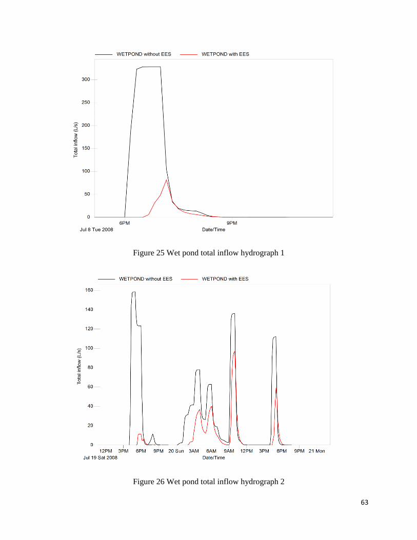
63
Figure 25 Wet pond total inflow hydrograph 1
Figure 26 Wet pond total inflow hydrograph 2
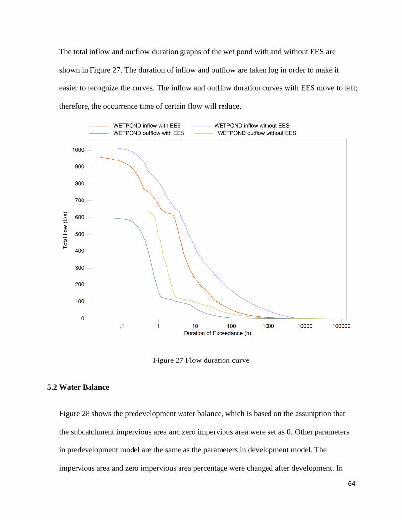
64
The total inflow and outflow duration graphs of the wet pond with and without EES are
shown in Figure 27. The duration of inflow and outflow are taken log in order to make it
easier to recognize the curves. The inflow and outflow duration curves with EES move to left;
therefore, the occurrence time of certain flow will reduce.
Figure 27 Flow duration curve
5.2 Water Balance
Figure 28 shows the predevelopment water balance, which is based on the assumption that
the subcatchment impervious area and zero impervious area were set as 0. Other parameters
in predevelopment model are the same as the parameters in development model. The
impervious area and zero impervious area percentage were changed after development. In

65
SWMM, the Hargreaves method to calculate the evaporation rate. (Hargreaves & Z.A., 1985)
Since the soil is sandy loam, the rain will percolate faster and evaporation rate is low.
Therefore, total infiltration is much more than total evaporation. After urbanization, there
will be more impervious area where evaporation rate will be higher than that of the sandy
loam pervious area before development.
Figure 28 Predevelopment water balance
Water balance of the case study site after development with only wet pond is shown in Figure
29. In this condition, 54% of the precipitation was infiltrated, 18% was evaporated and 28%
became surface runoff.
0%1%
99%
Predevelopment Water Balance
Evaporation
Surface Runoff
Total Infiltration
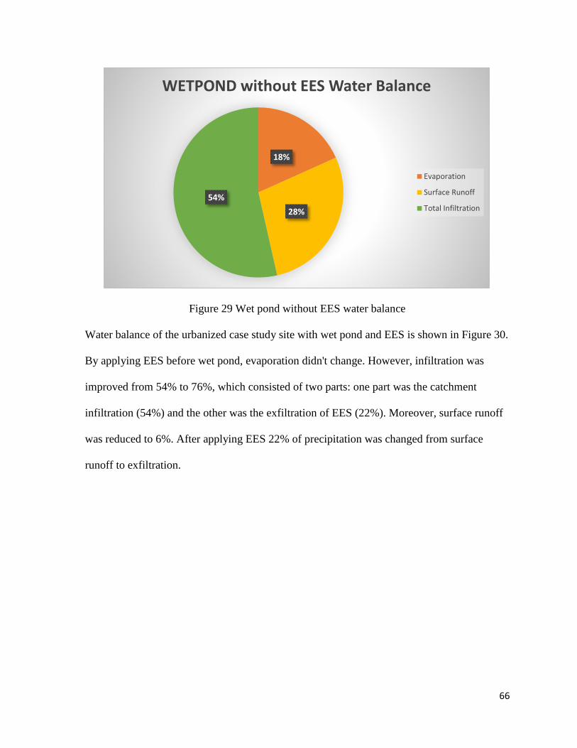
66
Figure 29 Wet pond without EES water balance
Water balance of the urbanized case study site with wet pond and EES is shown in Figure 30.
By applying EES before wet pond, evaporation didn't change. However, infiltration was
improved from 54% to 76%, which consisted of two parts: one part was the catchment
infiltration (54%) and the other was the exfiltration of EES (22%). Moreover, surface runoff
was reduced to 6%. After applying EES 22% of precipitation was changed from surface
runoff to exfiltration.
18%
28%
54%
WETPOND without EES Water Balance
Evaporation
Surface Runoff
Total Infiltration
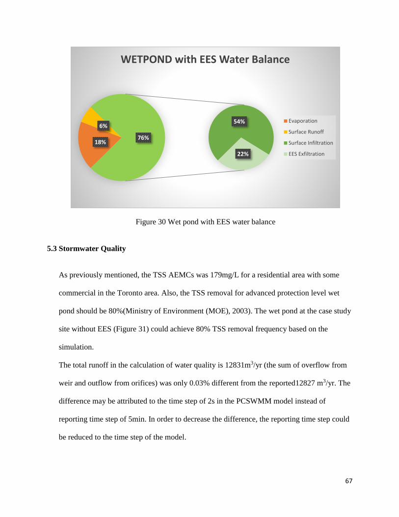
67
Figure 30 Wet pond with EES water balance
5.3 Stormwater Quality
As previously mentioned, the TSS AEMCs was 179mg/L for a residential area with some
commercial in the Toronto area. Also, the TSS removal for advanced protection level wet
pond should be 80%(Ministry of Environment (MOE), 2003). The wet pond at the case study
site without EES (Figure 31) could achieve 80% TSS removal frequency based on the
simulation.
The total runoff in the calculation of water quality is 12831m3/yr (the sum of overflow from
weir and outflow from orifices) was only 0.03% different from the reported12827 m3/yr. The
difference may be attributed to the time step of 2s in the PCSWMM model instead of
reporting time step of 5min. In order to decrease the difference, the reporting time step could
be reduced to the time step of the model.
18%
6%54%
22%
76%
WETPOND with EES Water Balance
Evaporation
Surface Runoff
Surface Infiltration
EES Exfiltration
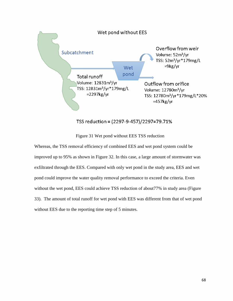
68
Figure 31 Wet pond without EES TSS reduction
Whereas, the TSS removal efficiency of combined EES and wet pond system could be
improved up to 95% as shown in Figure 32. In this case, a large amount of stormwater was
exfiltrated through the EES. Compared with only wet pond in the study area, EES and wet
pond could improve the water quality removal performance to exceed the criteria. Even
without the wet pond, EES could achieve TSS reduction of about77% in study area (Figure
33). The amount of total runoff for wet pond with EES was different from that of wet pond
without EES due to the reporting time step of 5 minutes.
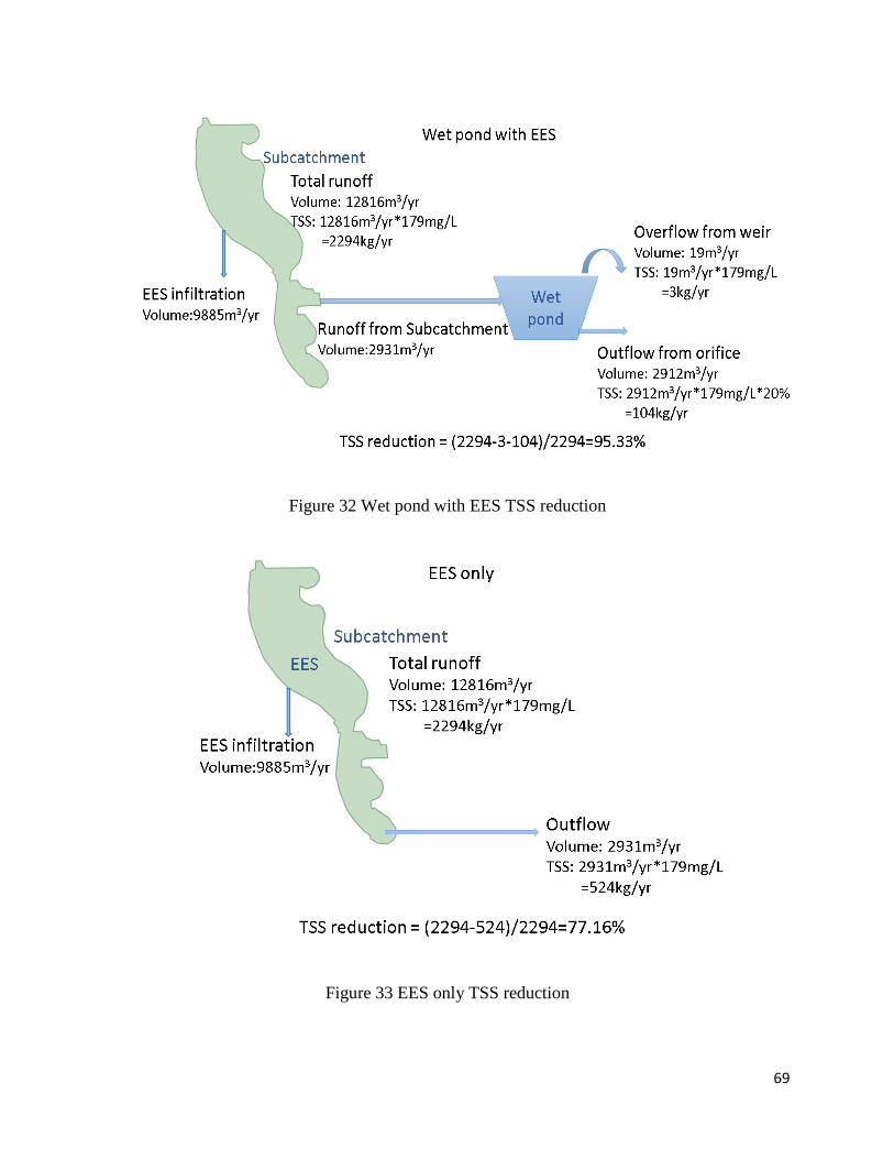
69
Figure 32 Wet pond with EES TSS reduction
Figure 33 EES only TSS reduction

70
Chapter 6 Conclusion and Recommendations
6.1 Conclusions
This research mainly focused on modelling EES. Based on the investigation, the following
conclusions are drawn.
Four modelling approaches were tested which include the MIDUSS event based model and four
options in PCSWMM model. It was found that the Orifice-Pump-Storage method in PCSWMM
was the best approach to model EES.
While analyzing EES performance over a single event using MIDUSS, runoff depths and
maximum intensities were expressively higher than 15mm and 50mm/hr (Ternier, 2012). In
order to investigate the long-term performance of EES with a wet pond, a case study was
conducted using the PCSWMM over 53-year rainfalls. Compared to the single event results, EES
didn’t perform that well for every single event throughout 53 years.
The case study also showed EES could meet the three criteria of stormwater management. The
average runoff volume reduction of EES was 9885m3/yr over 53 years, which was attributed to
exfiltration. Thus 28% of precipitation was reduced to 6% and turned into exfiltration. By
applying EES with wet pond, the long-term average TSS removal frequency was also improved
up to 95%.
6.2 Recommendations
In this research, EES performs as a LID practice; meeting the stormwater management criteria of
water volume and water balance. However, further research is still required with regard to EES

71
TSS removal mechanisms. Moreover, other pollutants should also be investigated with regard to
groundwater quality protection as water exfiltrating from EES flows directly to groundwater.
Additionally, EES was applied in every trench except the first and the last one in the study area.
The whole system may be optimized by the following further investigations:
Part of the EES in the storm sewer network can be removed instead of applying EES in
every trench to reduce the cost.
The location of the EES in a storm sewer network could be investigated for optimizing.
By applying EES, the wet pond size can be further reduced.
Wet pond standard may be revised if combined with EES.
Finally, by comparing the cost of applying EES with the cost of maintaining wet pond, better
decisions can be made about the feasibility of applying EES.

72
References
A.M. Candaras Associates Inc. (1997). Post-Constructyion Evaluation of Stormwater
Exfiltration & Filtration Systems. Etobicoke,Ontario: Queen's Printer for Ontario.
Binstock, M. (2011). Greening Stormwater Management in Ontario: An Analysis of Challenges
and Opportunities. Urban Ecosystems .
Bradford, A., & Gharabaghi, B. (2004). Evolution of Ontario's Stormwater Management
Planning and Design Guidance. Water Quality Resource Journal , 39 (4), 343-355.
Brown, R., Line, D., & Hunt, W. (2012, June). LID Treatment Train: Previous Concrete with
Subsurface Storage in Series with Bioretention and Care with Seasonal High Water Tables.
Journal of Environmental Engineering , 689-697.
Center for Watershed Protection. (1998). Better Site Design: A Handbook for Changing
Development Rules in Your Community. Ellicott City, Maryland.
Chapman, L., & Putman, D. (1983). The Physiography of Southern Ontario, 3rd Edition.
Ontario Geological Survery, Special Volume 2.
Chmakova, A. S. (2007). Environmental Assessment of Stormwater Pond Impact on A Rouge
River Tributary. Theses and Dissertations Paper317.
City of Etobicoke. (1992). Princess Margarete Boulevard Drawing PRB-1236-9-1.
City of Los Angeles. (2011). Development Best Management Practices Handbook- Low Impact
Development Manual Part B.
Credit Valley Conservation (CVC); Toronto and Region Conservation (TRCA). (2010). Low
Impact Development Stormwater management Planning and Design Guide.
Damodaram, C., Giacomoni, M. H., Khedun, C. P., Holmes, H., Ryan, A., Saour, W., et al.
(2010). Simulation of combined best management practices and Low Impact Development for
Sustainable Stormwater Management. Journal of the American Water Resources Association
(JAWRA) , 46 (5), 907-918.
Department of Environmental Resources. (1993). Design Manual For Use of Bioretention in
Stormwater Management. Department of Environmental Resources, Division of Environmental
Management, Watershed Protection Branch, Prince George's County, Maryland.
Dietz, M. E. (2007). Low Impact Development Practices: A Review of Current Research and
Recommendations for Future Directions. Water Air Soil Pollution , 186, 351-363.
Dmodaram, C., Giacomoni, M. H., C. Prakash Khedun, H. H., Ryan, A., Saour, W., & Zechman,
E. M. (2010). Simulation of Combined Best Management Practices and Low Impact
Development for Sustainable Stormwater Management. Journal of the American Water
Resources Association , 46 (5), 907-918.

73
Government of South Australia Adelaide. (2009). Water Sensitive Urban Design -Technical
Manual.
Groffman, P. M., & Crawford, M. K. (2003, May/June). Denitrification Potential in Urban
Riparian Zones. Journal of Environmental Quality , 1144-1149.
Hargreaves, G., & Z.A., S. (1985). Reference Crop Evapotranspiration from temperature.
Applied Engineering in Agriculture , 96-99.
Hollis, G. (1975). The Effect of Urbanization on Floods of Different Recurrence Interval.
Holman-Dodds, J. K., Bradley, A. A., & Potter, K. W. (2003, February). Evaluation of
Hydrologic Benefits of Infiltration Based Urban Stormwater Management. Journal of the
American Water Resources Association , 205-215.
2008Hydrologic Bioretention Performance and Design Criteria For Cold Climates
James, W. (2005). Rules for Responsible Modeling- 4th Edition. Guelph,Ontario: CHI .
Johengen, T. H., & LaRock, P. A. (1993). Quantifying nutrient removal processes within a
constucted wetland designed to treat urban stormwater runoff. Ecological Engineering , 347-366.
Khowaja, Z. A. (2007). Development of Stormwater Exfiltration Systems. Thesis and
Dissertations. Paper 255.
Mayer, T., Marsalek, J., & Reyes, E. D. (1995). Nutrients and Metal Contaminants Status of
Urban Stormwater Ponds. Journal of lake and Reservoir Management .
McCutcheon, M., & Wride, D. (2013). Shades of Green: Using SWMM LID Controls to
Simulate Green Infrastructure. Pragmatic Modeling of Urban Water Systems, Monograph 21.
1996Metropolitan Toronto Waterfront Stormwater Quality Characterization Study
Ministry of Environment (MOE). (2003). Stormwater management planning and design manual.
Toronto,Ontario: Queen's Printer for Ontario.
Ministry of Environment and Climate Change. (2015, February). Interpretation Bulletin Ontario
Ministry of Environment and Climate Change Expectations Re Stormwater Management.
Newcomer, M. E., Gurdak, J. J., Sklar, L. S., & Nanus, L. (2014). Urban recharge beneath low
impact development and effects of climate variability and change. Water Resources Research ,
pp. 1716-1734.
Oberts, G. (2000). Influence of Snowmelt Dynamics on Stormwater Runoff quality. Watershed
Protection Techniques , 1 (2), 55-61.
Olding, D. D., Steele, T. S., & Nemeth, J. C. (2004). Operational Monitoring of Urban
Stormwater Management Facilities and Receiving Subwatersheds in Richmond Hill, Ontario.
Water Quality Resource Journal , 39 (4), pp. 392-405.
Ontario Concrete Pipe Association (OCPA). (1997). Concrete Pipe Design Manual.

74
Open Data. (2011). Retrieved from York Region: http://www.york.ca/opendatalist/
Pazwash, H. (2011). Urban Stormwater Management. Taylor and Francis Group, LLC.
Richard, R. (2013). Investigation of The Sediment Removal Frequency For Wet-detention
Stormwater Management Ponds. Toronto, Ontario.
Roseen, R., Ballestero, T., Houle, J., Avelleaneda, P., Briggs, J., Fowler, G., et al. (2009).
Seasonal Performance Variaations for Stormwater Management Systems in Cold Climate
Conditions. Journal of Environmental Engineering , 135 (3), 128-137.
Rossman, L. A. (2008). Stormwater Management model User's Manual Version 5.0. Water
Supply and Water Resources Division National Risk Managment Reaearch Laboratory,
Cincinnati,ON.
Sanderson, M. (2004). Weather and Climate in Southern Ontario. University of Waterloo,
Department of Geography, Waterloo.
Stormwater Assessment Monitoring and Perfomance Program. (2004). Performance Assessment
of A Perforated Pipe Stormwater Exfiltration System. Toronto, ON: Toronto and Region
Conservation Authority.
Ternier, S. (2012). Review of Stormwater Management In Ontario And A Case Study On the
Etobicoke Exfiltration System. Thesis, Ryerson University, Environmental Applied Science and
Management, Toronto, Ontario.
The Municipal Infrastructure Group Ltd.; Schollen & Company Inc. (2011). Stormwater
Management Feasibility Study. Toronto,Ontario.
Toronto and Region Conservation. (2006). Performance Evaluation of Permeable Pavement and
A Bioretention Swale. Seneca College; King City, Ontario. Toronto and Region Conservartion
Authority, Interim Report #2.
Toronto and Region Conservation. (2007). Rouge River Watershed Plan Towards A Healthy And
Sustainable Future. Toronto, ON.
Toronto and Region Conservation. (2012). Stormwater Management Criteria. Retrieved from
http://www.trca.on.ca/the-living-city/water-flood-management/storm-water-management.dot
Town of Richmond Hill. (2008, Feburary 26). Engineering & Public Work Design &
Construction.
Town of Richmond Hill. (1998). Richmond Hill Standards and Specifications Manual.
Richmond Hill, Ontario.
Tran, J., & Li, J. (2015). Planning and Design Manual of the Etobicoke Exfiltration System for
Stormwater Management. Toronto.
Tsihrintzis, V. A., & Hamid, R. (1997). Modeling and Management of Urban Stormwater Runoff
Quality: A Review. Water Resources Management , 137-164.

75
United States Environmental Protection Agency (US EPA). (2000). Low Impact Development
(LID)- A Literature Review. Office of Water (4203), Washington DC.
United States Environmental Protection Agency (US EPA). (1999). Preliminary Data Summary
of Urban Stormwater Best Management Practices. Office of Water.
United States Environmental Protection Agency. (2007). Reducing Stormwater Costs through
Low Impact Development (LID) Strategies and Practices. Nonpoint Source Control Branch,
Washington DC.
US Department of Transportation. Retention, Detention and Overland Flow for Pollutant
Removal from Highway Stormwater Runoff, volume I: Research Report. U.S. Department of
Transportation, Federal Highway Administration.
Villarreal, E. L., & Bengtsson, A. S.-D. (2004). Inner City Stormwater Contorl Using A
Combination of Best Management Practices. Ecological Engineering , 279-298.
Wahl, M., McKellar, H., & Williams, T. Patterns of Nutrient Loading in Forested and Urbanized
Coastal Streams. Journal of Excperimental Marine Biology and Ecology , 213, 111-131.
Wong, T. (2006). An Overview of Water Sensitive Urban Design Practices in Australia. Water
Practice & Technology , 1 (1).
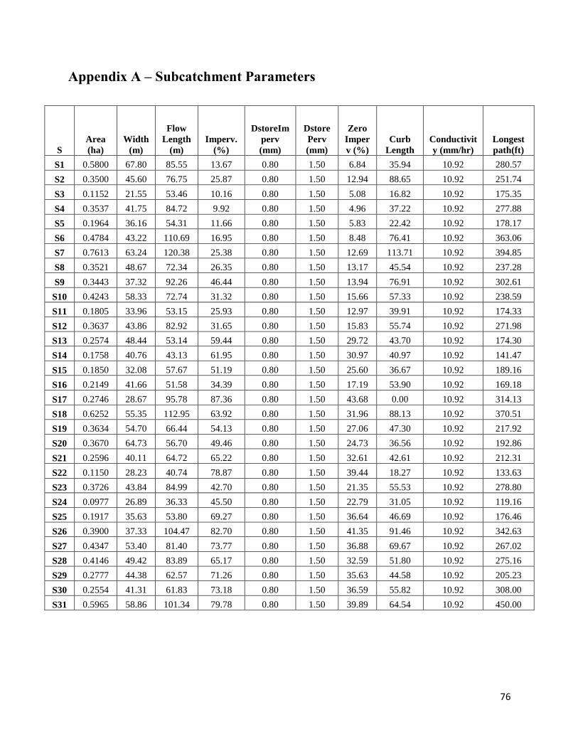
76
Appendix A – Subcatchment Parameters
S
Area
(ha)
Width
(m)
Flow
Length
(m)
Imperv.
(%)
DstoreIm
perv
(mm)
Dstore
Perv
(mm)
Zero
Imper
v (%)
Curb
Length
Conductivit
y (mm/hr)
Longest
path(ft)
S1 0.5800 67.80 85.55 13.67 0.80 1.50 6.84 35.94 10.92 280.57
S2 0.3500 45.60 76.75 25.87 0.80 1.50 12.94 88.65 10.92 251.74
S3 0.1152 21.55 53.46 10.16 0.80 1.50 5.08 16.82 10.92 175.35
S4 0.3537 41.75 84.72 9.92 0.80 1.50 4.96 37.22 10.92 277.88
S5 0.1964 36.16 54.31 11.66 0.80 1.50 5.83 22.42 10.92 178.17
S6 0.4784 43.22 110.69 16.95 0.80 1.50 8.48 76.41 10.92 363.06
S7 0.7613 63.24 120.38 25.38 0.80 1.50 12.69 113.71 10.92 394.85
S8 0.3521 48.67 72.34 26.35 0.80 1.50 13.17 45.54 10.92 237.28
S9 0.3443 37.32 92.26 46.44 0.80 1.50 13.94 76.91 10.92 302.61
S10 0.4243 58.33 72.74 31.32 0.80 1.50 15.66 57.33 10.92 238.59
S11 0.1805 33.96 53.15 25.93 0.80 1.50 12.97 39.91 10.92 174.33
S12 0.3637 43.86 82.92 31.65 0.80 1.50 15.83 55.74 10.92 271.98
S13 0.2574 48.44 53.14 59.44 0.80 1.50 29.72 43.70 10.92 174.30
S14 0.1758 40.76 43.13 61.95 0.80 1.50 30.97 40.97 10.92 141.47
S15 0.1850 32.08 57.67 51.19 0.80 1.50 25.60 36.67 10.92 189.16
S16 0.2149 41.66 51.58 34.39 0.80 1.50 17.19 53.90 10.92 169.18
S17 0.2746 28.67 95.78 87.36 0.80 1.50 43.68 0.00 10.92 314.13
S18 0.6252 55.35 112.95 63.92 0.80 1.50 31.96 88.13 10.92 370.51
S19 0.3634 54.70 66.44 54.13 0.80 1.50 27.06 47.30 10.92 217.92
S20 0.3670 64.73 56.70 49.46 0.80 1.50 24.73 36.56 10.92 192.86
S21 0.2596 40.11 64.72 65.22 0.80 1.50 32.61 42.61 10.92 212.31
S22 0.1150 28.23 40.74 78.87 0.80 1.50 39.44 18.27 10.92 133.63
S23 0.3726 43.84 84.99 42.70 0.80 1.50 21.35 55.53 10.92 278.80
S24 0.0977 26.89 36.33 45.50 0.80 1.50 22.79 31.05 10.92 119.16
S25 0.1917 35.63 53.80 69.27 0.80 1.50 36.64 46.69 10.92 176.46
S26 0.3900 37.33 104.47 82.70 0.80 1.50 41.35 91.46 10.92 342.63
S27 0.4347 53.40 81.40 73.77 0.80 1.50 36.88 69.67 10.92 267.02
S28 0.4146 49.42 83.89 65.17 0.80 1.50 32.59 51.80 10.92 275.16
S29 0.2777 44.38 62.57 71.26 0.80 1.50 35.63 44.58 10.92 205.23
S30 0.2554 41.31 61.83 73.18 0.80 1.50 36.59 55.82 10.92 308.00
S31 0.5965 58.86 101.34 79.78 0.80 1.50 39.89 64.54 10.92 450.00
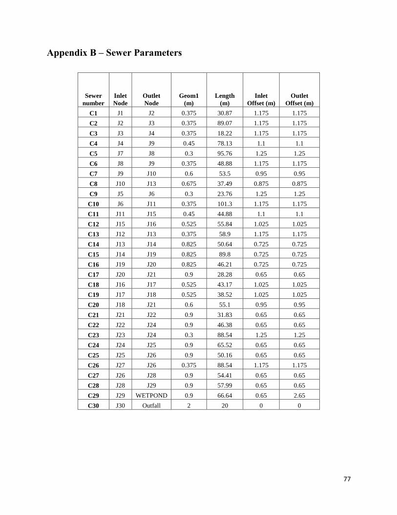
77
Appendix B – Sewer Parameters
Sewer
number
Inlet
Node
Outlet
Node
Geom1
(m)
Length
(m)
Inlet
Offset (m)
Outlet
Offset (m)
C1 J1 J2 0.375 30.87 1.175 1.175
C2 J2 J3 0.375 89.07 1.175 1.175
C3 J3 J4 0.375 18.22 1.175 1.175
C4 J4 J9 0.45 78.13 1.1 1.1
C5 J7 J8 0.3 95.76 1.25 1.25
C6 J8 J9 0.375 48.88 1.175 1.175
C7 J9 J10 0.6 53.5 0.95 0.95
C8 J10 J13 0.675 37.49 0.875 0.875
C9 J5 J6 0.3 23.76 1.25 1.25
C10 J6 J11 0.375 101.3 1.175 1.175
C11 J11 J15 0.45 44.88 1.1 1.1
C12 J15 J16 0.525 55.84 1.025 1.025
C13 J12 J13 0.375 58.9 1.175 1.175
C14 J13 J14 0.825 50.64 0.725 0.725
C15 J14 J19 0.825 89.8 0.725 0.725
C16 J19 J20 0.825 46.21 0.725 0.725
C17 J20 J21 0.9 28.28 0.65 0.65
C18 J16 J17 0.525 43.17 1.025 1.025
C19 J17 J18 0.525 38.52 1.025 1.025
C20 J18 J21 0.6 55.1 0.95 0.95
C21 J21 J22 0.9 31.83 0.65 0.65
C22 J22 J24 0.9 46.38 0.65 0.65
C23 J23 J24 0.3 88.54 1.25 1.25
C24 J24 J25 0.9 65.52 0.65 0.65
C25 J25 J26 0.9 50.16 0.65 0.65
C26 J27 J26 0.375 88.54 1.175 1.175
C27 J26 J28 0.9 54.41 0.65 0.65
C28 J28 J29 0.9 57.99 0.65 0.65
C29 J29 WETPOND 0.9 66.64 0.65 2.65
C30 J30 Outfall 2 20 0 0
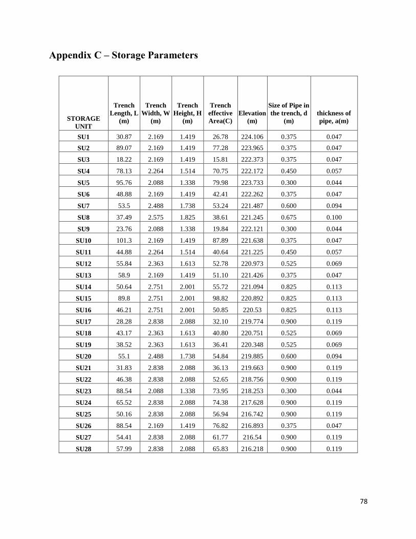
78
Appendix C – Storage Parameters
STORAGE
UNIT
Trench
Length, L
(m)
Trench
Width, W
(m)
Trench
Height, H
(m)
Trench
effective
Area(C)
Elevation
(m)
Size of Pipe in
the trench, d
(m)
thickness of
pipe, a(m)
SU1 30.87 2.169 1.419 26.78 224.106 0.375 0.047
SU2 89.07 2.169 1.419 77.28 223.965 0.375 0.047
SU3 18.22 2.169 1.419 15.81 222.373 0.375 0.047
SU4 78.13 2.264 1.514 70.75 222.172 0.450 0.057
SU5 95.76 2.088 1.338 79.98 223.733 0.300 0.044
SU6 48.88 2.169 1.419 42.41 222.262 0.375 0.047
SU7 53.5 2.488 1.738 53.24 221.487 0.600 0.094
SU8 37.49 2.575 1.825 38.61 221.245 0.675 0.100
SU9 23.76 2.088 1.338 19.84 222.121 0.300 0.044
SU10 101.3 2.169 1.419 87.89 221.638 0.375 0.047
SU11 44.88 2.264 1.514 40.64 221.225 0.450 0.057
SU12 55.84 2.363 1.613 52.78 220.973 0.525 0.069
SU13 58.9 2.169 1.419 51.10 221.426 0.375 0.047
SU14 50.64 2.751 2.001 55.72 221.094 0.825 0.113
SU15 89.8 2.751 2.001 98.82 220.892 0.825 0.113
SU16 46.21 2.751 2.001 50.85 220.53 0.825 0.113
SU17 28.28 2.838 2.088 32.10 219.774 0.900 0.119
SU18 43.17 2.363 1.613 40.80 220.751 0.525 0.069
SU19 38.52 2.363 1.613 36.41 220.348 0.525 0.069
SU20 55.1 2.488 1.738 54.84 219.885 0.600 0.094
SU21 31.83 2.838 2.088 36.13 219.663 0.900 0.119
SU22 46.38 2.838 2.088 52.65 218.756 0.900 0.119
SU23 88.54 2.088 1.338 73.95 218.253 0.300 0.044
SU24 65.52 2.838 2.088 74.38 217.628 0.900 0.119
SU25 50.16 2.838 2.088 56.94 216.742 0.900 0.119
SU26 88.54 2.169 1.419 76.82 216.893 0.375 0.047
SU27 54.41 2.838 2.088 61.77 216.54 0.900 0.119
SU28 57.99 2.838 2.088 65.83 216.218 0.900 0.119

79
Appendix D - Junction Parameter Summary
Junction
Number
Junction
bottom El.
(m)
Junction
ground
El. (m)
Junction
Depth (m)
J1 224.63 227.36 2.73
J2 224.49 227.22 2.73
J3 222.90 225.63 2.73
J4 222.62 225.43 2.81
J5 222.72 225.82 3.10
J6 222.16 225.34 3.18
J7 224.33 226.99 2.66
J8 222.79 225.52 2.73
J9 221.79 224.75 2.96
J10 221.47 224.50 3.03
J11 221.68 224.95 3.27
J12 221.95 224.83 2.88
J13 221.22 224.10 2.88
J14 220.97 224.44 3.47
J15 221.35 224.70 3.35
J16 221.13 224.55 3.42
J17 220.72 224.14 3.42
J18 220.19 223.68 3.49
J19 220.61 224.54 3.93
J20 219.77 223.77 4.00
J21 219.66 223.72 4.06
J22 218.76 222.82 4.06
J23 218.85 222.31 3.46
J24 217.63 221.69 4.06
J25 216.74 220.80 4.06
J26 216.54 220.60 4.06
J27 217.42 220.28 2.86
J28 216.22 219.60 3.38
J29 215.46 218.84 3.38
J30 213.07 213.07 0.00
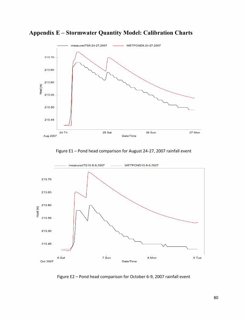
80
Appendix E – Stormwater Quantity Model: Calibration Charts
Figure E1 – Pond head comparison for August 24-27, 2007 rainfall event
Figure E2 – Pond head comparison for October 6-9, 2007 rainfall event
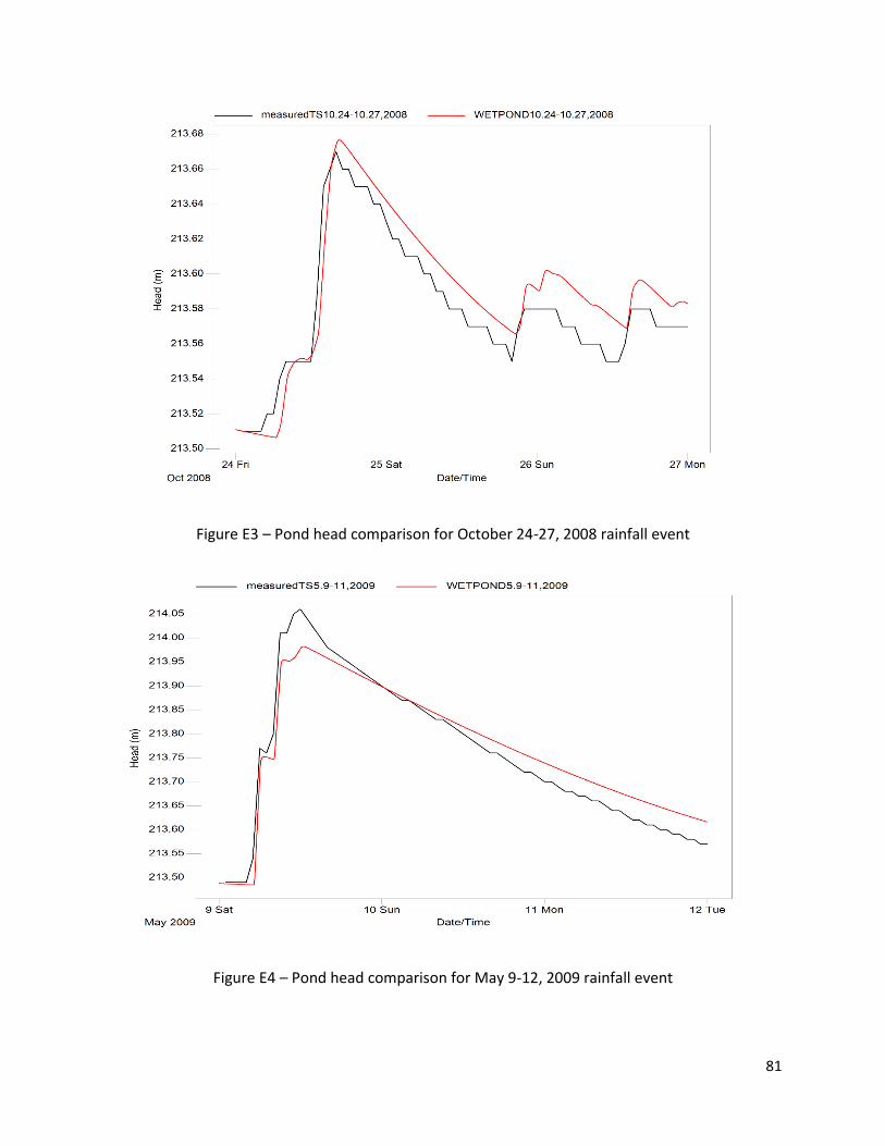
81
Figure E3 – Pond head comparison for October 24-27, 2008 rainfall event
Figure E4 – Pond head comparison for May 9-12, 2009 rainfall event

82
Appendix F – Rainfall Data-By Descending Total Record Data
Figure F1 Rainfall data - by descending total record data (Whole year)
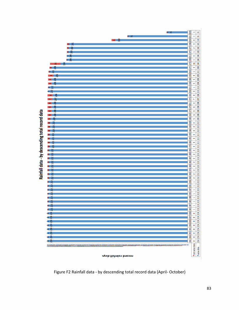
83
Figure F2 Rainfall data - by descending total record data (April- October)
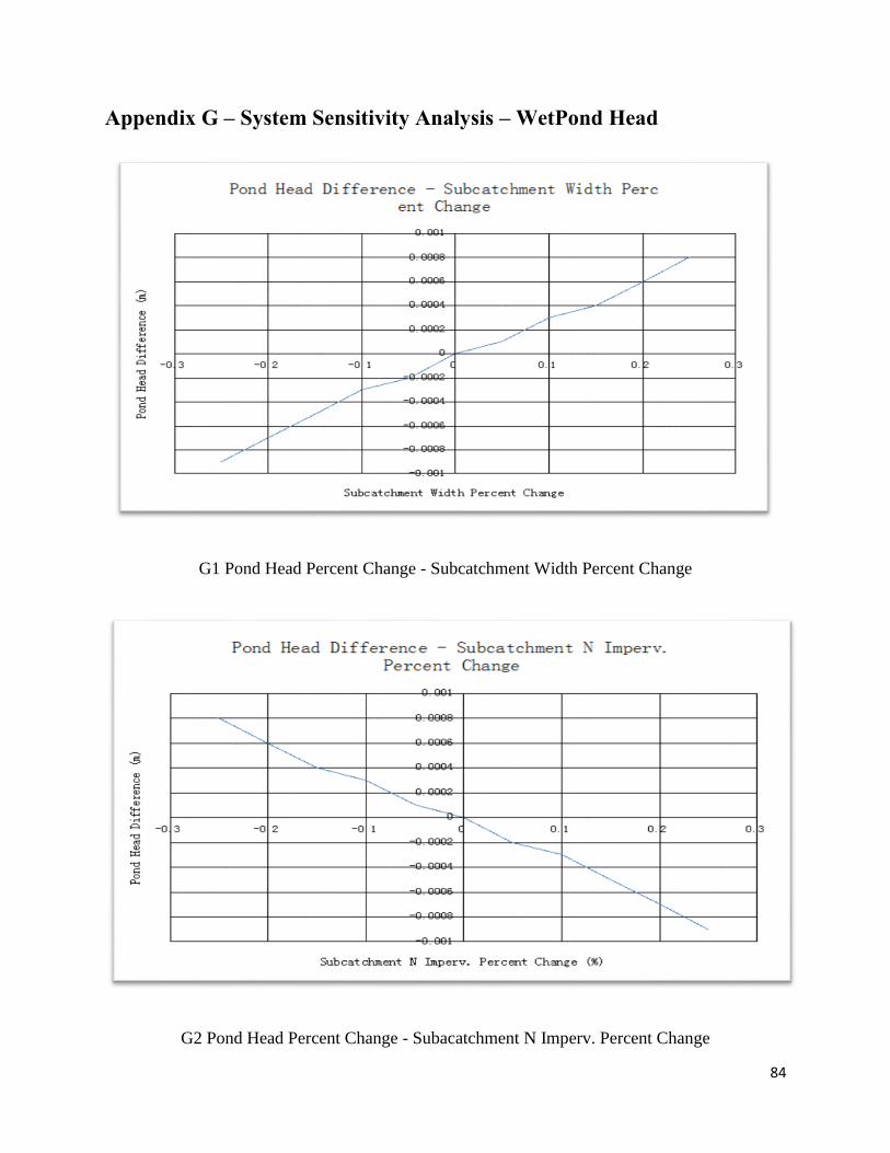
84
Appendix G – System Sensitivity Analysis – WetPond Head
G1 Pond Head Percent Change - Subcatchment Width Percent Change
G2 Pond Head Percent Change - Subacatchment N Imperv. Percent Change
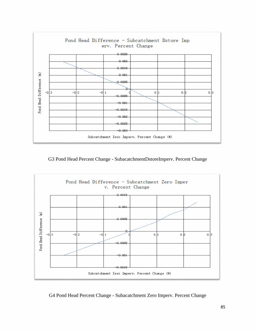
85
G3 Pond Head Percent Change - SubacatchmentDstoreImperv. Percent Change
G4 Pond Head Percent Change - Subacatchment Zero Imperv. Percent Change
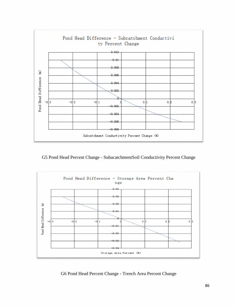
86
G5 Pond Head Percent Change - SubacatchmentSoil Conductivity Percent Change
G6 Pond Head Percent Change - Trench Area Percent Change
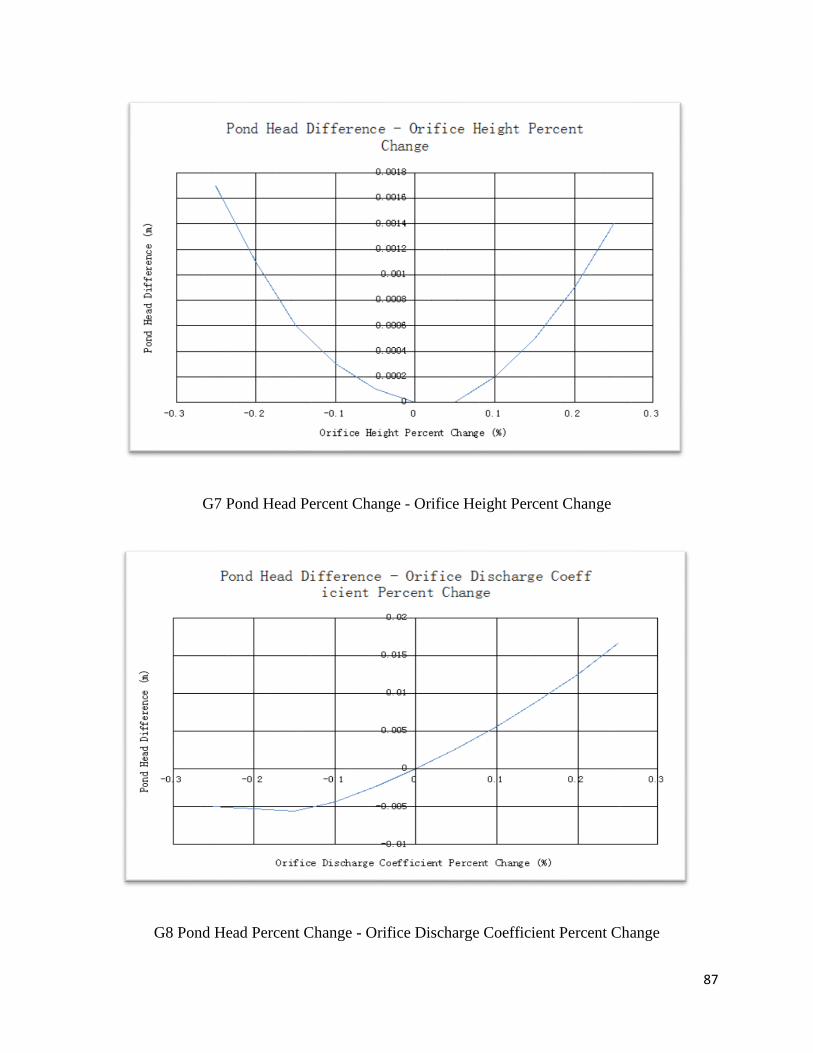
87
G7 Pond Head Percent Change - Orifice Height Percent Change
G8 Pond Head Percent Change - Orifice Discharge Coefficient Percent Change
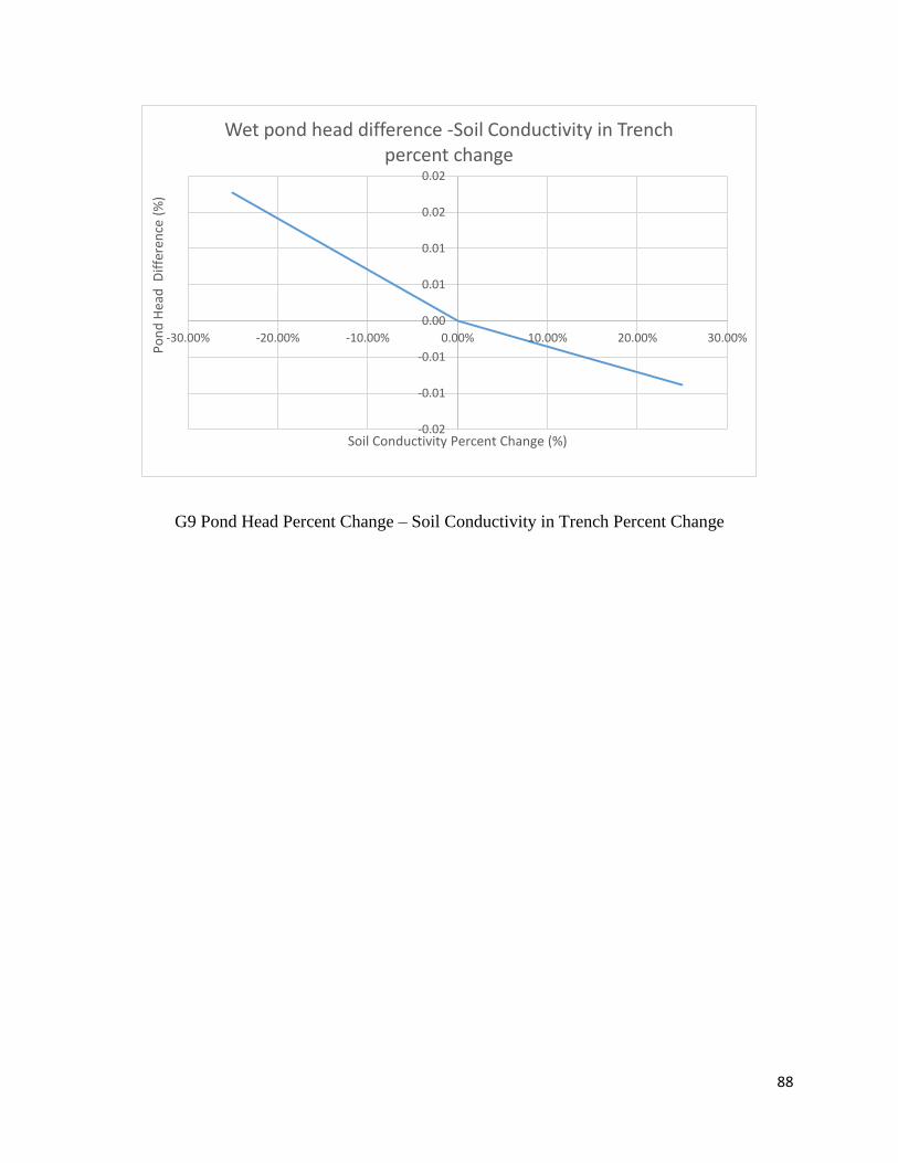
88
G9 Pond Head Percent Change – Soil Conductivity in Trench Percent Change
-0.02
-0.01
-0.01
0.00
0.01
0.01
0.02
0.02
-30.00% -20.00% -10.00% 0.00% 10.00% 20.00% 30.00%
Po
nd
Hea
d D
iffe
ren
ce (
%)
Soil Conductivity Percent Change (%)
Wet pond head difference -Soil Conductivity in Trench percent change
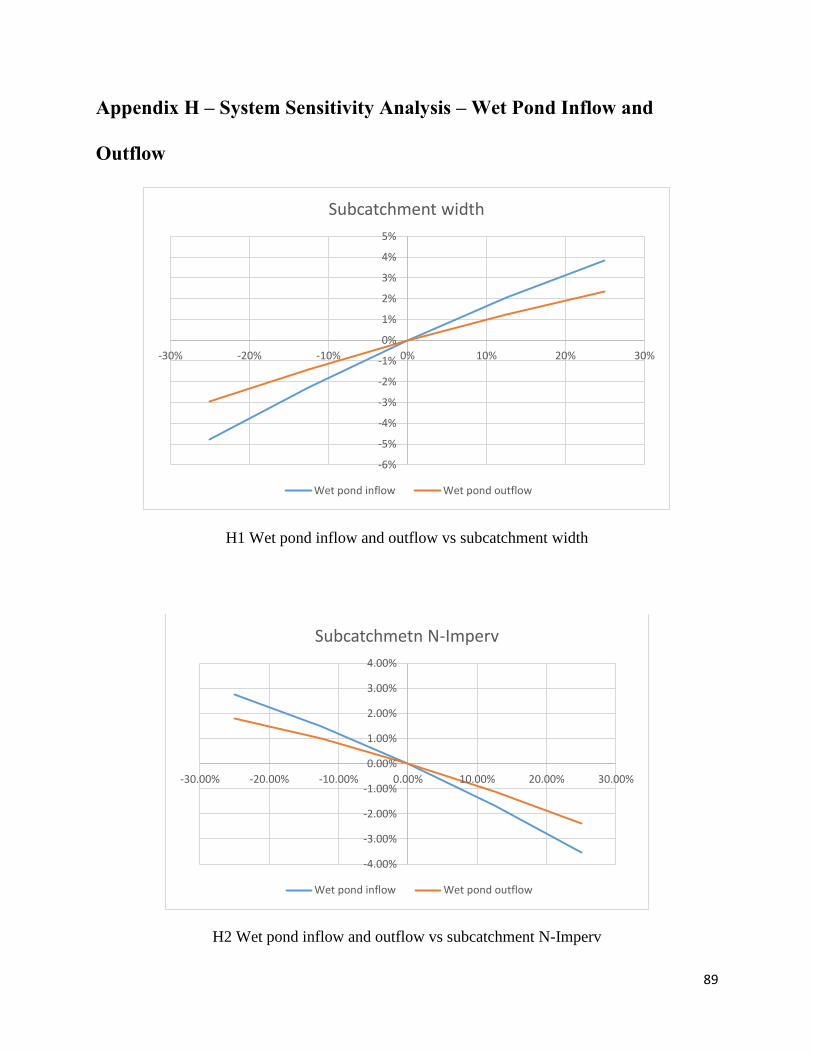
89
Appendix H – System Sensitivity Analysis – Wet Pond Inflow and
Outflow
H1 Wet pond inflow and outflow vs subcatchment width
H2 Wet pond inflow and outflow vs subcatchment N-Imperv
-6%
-5%
-4%
-3%
-2%
-1%
0%
1%
2%
3%
4%
5%
-30% -20% -10% 0% 10% 20% 30%
Subcatchment width
Wet pond inflow Wet pond outflow
-4.00%
-3.00%
-2.00%
-1.00%
0.00%
1.00%
2.00%
3.00%
4.00%
-30.00% -20.00% -10.00% 0.00% 10.00% 20.00% 30.00%
Subcatchmetn N-Imperv
Wet pond inflow Wet pond outflow
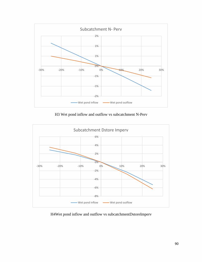
90
H3 Wet pond inflow and outflow vs subcatchment N-Perv
H4Wet pond inflow and outflow vs subcatchmentDstoreImperv
-2%
-1%
-1%
0%
1%
1%
2%
-30% -20% -10% 0% 10% 20% 30%
Subcatchment N- Perv
Wet pond inflow Wet pond outflow
-8%
-6%
-4%
-2%
0%
2%
4%
6%
-30% -20% -10% 0% 10% 20% 30%
Subcatchment Dstore Imperv
Wet pond inflow Wet pond outflow
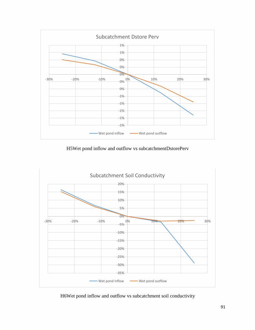
91
H5Wet pond inflow and outflow vs subcatchmentDstorePerv
H6Wet pond inflow and outflow vs subcatchment soil conductivity
-1%
-1%
-1%
-1%
-1%
0%
0%
0%
0%
0%
1%
1%
-30% -20% -10% 0% 10% 20% 30%
Subcatchment Dstore Perv
Wet pond inlfow Wet pond outflow
-35%
-30%
-25%
-20%
-15%
-10%
-5%
0%
5%
10%
15%
20%
-30% -20% -10% 0% 10% 20% 30%
Subcatchment Soil Conductivity
Wet pond inflow Wet pond outflow
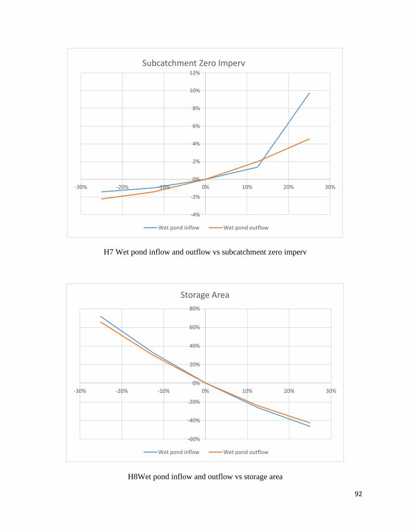
92
H7 Wet pond inflow and outflow vs subcatchment zero imperv
H8Wet pond inflow and outflow vs storage area
-4%
-2%
0%
2%
4%
6%
8%
10%
12%
-30% -20% -10% 0% 10% 20% 30%
Subcatchment Zero Imperv
Wet pond inlfow Wet pond outflow
-60%
-40%
-20%
0%
20%
40%
60%
80%
-30% -20% -10% 0% 10% 20% 30%
Storage Area
Wet pond inflow Wet pond outflow
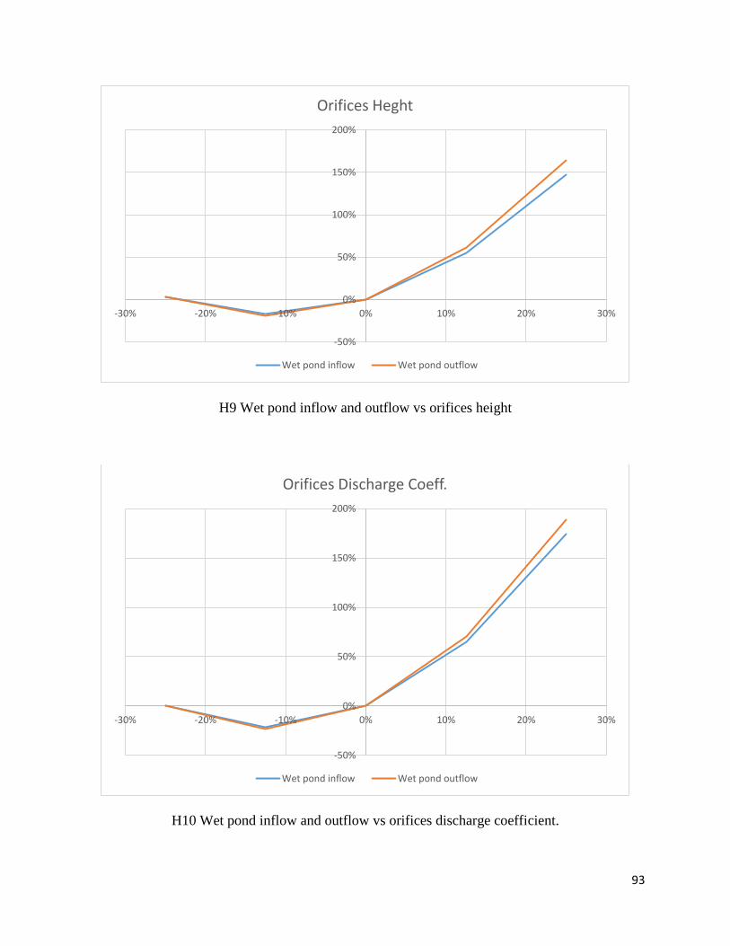
93
H9 Wet pond inflow and outflow vs orifices height
H10 Wet pond inflow and outflow vs orifices discharge coefficient.
-50%
0%
50%
100%
150%
200%
-30% -20% -10% 0% 10% 20% 30%
Orifices Heght
Wet pond inflow Wet pond outflow
-50%
0%
50%
100%
150%
200%
-30% -20% -10% 0% 10% 20% 30%
Orifices Discharge Coeff.
Wet pond inflow Wet pond outflow
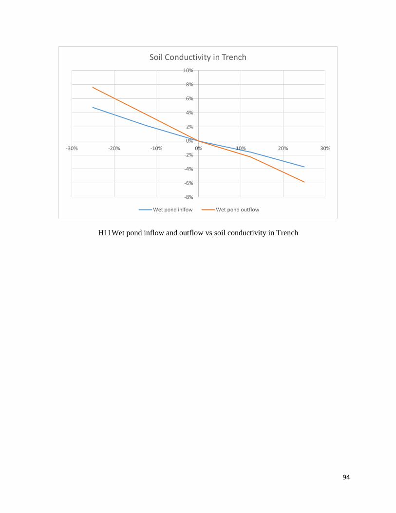
94
H11Wet pond inflow and outflow vs soil conductivity in Trench
-8%
-6%
-4%
-2%
0%
2%
4%
6%
8%
10%
-30% -20% -10% 0% 10% 20% 30%
Soil Conductivity in Trench
Wet pond inlfow Wet pond outflow