Long-Term Electricity Procurement for Large

Industrial Consumers Under Uncertainty

Qi Zhang,† Andreas M. Bremen,‡ Ignacio E. Grossmann,∗,† Arul

Sundaramoorthy,¶ and Jose M. Pinto§

†Center for Advanced Process Decision-making, Department of Chemical Engineering,

Carnegie Mellon University, Pittsburgh, PA 15213, USA

‡Faculty of Mechanical Engineering, RWTH Aachen University, 52056 Aachen, Germany

¶Business and Supply Chain Optimization R&D, Praxair, Inc., Tonawanda, NY 14150,

USA

§Business and Supply Chain Optimization R&D, Praxair, Inc., Danbury, CT 06810, USA

E-mail: grossmann@cmu.edu

Abstract

Due to the need of adjusting plant operations to time-varying electricity prices and

changing product demand, managing the procurement of electricity in power-intensive

businesses has become a major challenge. Large industrial electricity consumers often

enter into long-term contracts with favorable rates. However, such power contracts

require the consumers to commit themselves to the amount that they are going to pur-

chase months in advance when future demand is not yet known with certainty. In this

work, we simultaneously optimize long-term electricity procurement and production

planning while considering uncertainty in product demand. We propose a multiscale

multistage stochastic programming model in which a one-year planning horizon is di-

vided into seasons, with each season represented by two characteristic weeks; also, each

1

season corresponds to a stage at which the demand for that season is revealed. The pro-

gressive hedging algorithm is applied to solve industrially relevant large-scale instances

of the mixed-integer linear programming model. Moreover, two di�erent sets of non-

anticipativity constraints are proposed, which exhibit di�erent computational behavior.

We emphasize the use of the value of stochastic solution for multistage problems when

evaluating the bene�ts of the stochastic optimization, which are demonstrated in an

illustrative example as well as an industrial air separation case.

1 Introduction

Due to the increasing volatility in electricity prices and availability, cost-e�ective procure-

ment of electricity in power-intensive businesses has become a major challenge. Large in-

dustrial electricity consumers often enter into long-term bilateral power contracts with their

utilities, which o�er favorable rates for large purchases. Typically, such power contracts

require the consumers to commit themselves to the amount that they are going to purchase

months in advance. However, determining the optimal purchasing amount is challenging

since electricity demand is often very di�cult to predict due to the uncertainties associated

with industrial production processes.

Although many existing works address problems involving power contracts from an elec-

tricity producer's or retailer's point of view1�4, the literature is scarce in contributions con-

sidering the consumer's perspective. Conejo et al. 5 solve a medium-term electricity procure-

ment problem that considers a set of bilateral contracts, hourly changing spot prices, and

the possibility of producing electricity with an onsite generating facility. The self-generated

power can be used for own consumption or sold to the spot market. A subsequent work6

addresses a similar problem for a shorter time horizon, while considering cost volatility by

using an estimate of the covariance of the spot price. While the models proposed in these

two papers are deterministic, Carrión et al. 7 apply stochastic programming to explicitly

model uncertainty in electricity prices. Furthermore, the conditional value-at-risk (CVaR) is

2

included in the model as a measure of risk, which is used to show the clear trade-o� between

expected cost and risk. A similar trade-o� is shown by Zare et al. 8 who apply the concept

of information gap decision theory to evaluate the robustness of a solution against high spot

prices or high procurement costs. Beraldi et al. 9 consider the short-term electricity procure-

ment problem involving bilateral contracts and the day-ahead market under both electricity

price and demand uncertainty; here, a stochastic programming model is solved in a rolling

horizon fashion. A similar problem is considered by Beraldi et al. 10 , who further include the

CVaR in the stochastic programming formulation to account for risk.

All above-mentioned references do not consider the possibility of the consumers a�ecting

their own electricity demand by adjusting their electricity-consuming processes. This implies

that a separate production scheduling problem has to be solved �rst in order to determine the

electricity demand, which then can be used as input in the electricity procurement problem.

However, this sequential approach is likely to be suboptimal since the production scheduling

problem does not take electricity price information into account. As shown in many recent

works on industrial demand side management (DSM), considering time-sensitive electricity

prices can have a very signi�cant impact on the load pro�les of power-intensive industrial

processes. For more details on industrial DSM, we refer to a recent comprehensive literature

review by Zhang and Grossmann 11 .

Although it is clear that production and electricity procurement have to be coordinated in

order to achieve the most cost-e�ective solution, optimization frameworks integrating these

decisions have only been proposed very recently. For power-intensive continuous process

networks, Zhang et al. 12 propose a detailed production scheduling model that also includes

a block contract formulation, which can be used to model a large variety of power contracts.

Hadera et al. 13 consider multiple electricity sources as well as onsite generation, which gen-

erates electricity that can be either used to power the plant or sold to the electricity market.

Besides integrating production scheduling and electricity procurement, Zhang et al. 14 model

uncertainty in both electricity price and product demand by applying a two-stage stochastic

3

programming approach, and consider risk by incorporating the CVaR into the model. In

this case, an extensive analysis of the value of stochastic solution (VSS) led to an interesting

insight, namely that in risk-neutral optimization, accounting for electricity price uncertainty

does not result in any signi�cant bene�t, whereas in risk-averse optimization, modeling price

uncertainty is crucial for obtaining good solutions. In recent works on scheduling with provi-

sion of interruptible load15�17, uncertainty related to demand response events has also been

considered.

The vast majority of existing works on industrial DSM have tackled short-term prob-

lems11, typically considering time horizons of one day or one week. Very few attempts have

been made to solve long-term DSM problems. The challenge herein is the following: To

account for time-sensitive electricity prices, a detailed model with a �ne time discretization

(often on an hourly basis) is required. In long-term planning problems, the time horizon may

span multiple months or years. It is then computationally intractable to apply the �ne time

discretization to the entire time horizon; however, we also cannot simply use an aggregate

model with a coarse time discretization since then we would not be able to model time-

sensitive DSM activities. Mitra et al. 18 solve a stochastic capacity expansion problem over a

planning horizon of multiple years. The model is simpli�ed by leveraging the seasonality of

electricity prices. Here, each year is divided into four seasons, and each season is represented

by one week, which is repeated cyclically and characterized by a typical electricity price

pro�le that re�ects the price's seasonal behavior. In order to solve an integrated production

routing problem, Zhang et al. 19 propose an optimization framework involving two time grids,

a �ne one for production scheduling and a coarse one for distribution planning.

In this work, we solve a long-term integrated production planning and electricity pro-

curement problem while considering uncertainty in product demand. We apply a multiscale

modeling approach, similar to the one proposed by Mitra et al. 18 , and develop a mulstistage

stochastic programming formulation to model the uncertainty. For solving large-scale in-

stances of the model, we apply progressive hedging20, which allows the decomposition of the

4

full-space problem into subproblems, one for each scenario. In that context, we examine

the impact of alternative sets of non-anticipativity constraints on the computational perfor-

mance. Furthermore, when analyzing the results, we emphasize the use of the VSS, which

has seldom been considered for multistage problems in the literature, as the key measure for

assessing the bene�t of the stochastic optimization.

The remainder of this paper is organized as follows. After stating the problem in Section

2, the multiscale multistage stochastic model is developed in Section 3. In Section 4, we

de�ne the VSS for multistage problems and present the algorithm for computing it. The

progressive hedging algorithm for solving large-scale instances is presented in Section 5. We

apply the proposed framework to an illustrative example, as well as to a real-world industrial

case study for which the results are shown in Sections 6 and 7, respectively. Finally, in Section

8, we close with a summary of the results and concluding remarks.

2 Problem Statement

We consider process networks involving continuous processes that consume signi�cant amounts

of electric energy during operation. Here, a process can refer to a piece of equipment, a set

of multiple interconnected pieces of equipment, or an entire plant. The processes in such

a network di�er in their feeds and products, restrictions on the production rates, process

dynamics, and power consumption characteristics. Inventory capacities are given for storable

intermediate and �nal products. It is assumed that the variable operating cost only consists

of electricity cost, inventory cost, and the cost of purchasing additional products.

Electricity can be purchased from an annual power contract, seasonal power contracts

(one for each season), and the spot market. The annual contract o�ers a �xed price that

does not change over time; however, the consumer has to commit to the purchase amount

before the start of the year and has to maintain a constant electricity purchase from this con-

tract throughout the year. Seasonal contracts apply time-of-use (TOU) prices; the purchase

5

amount for the corresponding season has to be announced at the beginning of the season.

Electricity purchase from the spot market is subject to �uctuating prices, but can be made

a day in advance (day-ahead market) or on the spot (real-time market).

The product demand is uncertain; however, probability information is given, and it can

be assumed that the product demand for each season will be known at the beginning of the

season. This is in most cases a valid assumption since most commodity products require a

pre-order period; also, slight demand changes within a season can be handled with existing

produce inventory.

The goal is to optimize the production and electricity procurement decisions over a plan-

ning horizon of one year. For any time point of the planning horizon, depending on the

realization of the uncertainty up to that point, we determine:

• the mode of operation for each process,

• the processing rate in each process,

• the amounts of products stored,

• the amounts of products purchased,

• the amount of electricity purchased from each source.

3 Model Formulation

We propose a discrete-time mixed-integer linear programming (MILP) planning model that is

based on a mode-based formulation developed by Zhang et al. 12 . In the following, we omit a

detailed description of the scheduling constraints, which can be found in the original paper12,

and focus on the new modeling aspects related to the multiscale time representation and

the multistage stochastic programming formulation. Note that unless speci�ed otherwise,

continuous variables in this model are constrained to be nonnegative. A list of indices,

6

sets, parameters, and variables used in the model formulation is given in the Nomenclature

section.

3.1 Multiscale Time Representation

In order to capture the impact of time-sensitive electricity prices without applying a �ne time

discretization to the entire planning horizon, we propose a multiscale representation of time,

which is illustrated in Figure 1. The planning horizon (here one year) is divided into seasons,

where each season, denoted by the index h, is represented by two weeks (index k). Each

week is divided into time periods of equal length, ∆t (typically an hour). The scheduling

horizon in week k of season h is de�ned by the set of time periods T hk = {1, 2, . . . , tkh}, where

T hk is a subset of Thk = {−θmax + 1,−θmax + 2, . . . , 0, 1, . . . , tkh}.

Week Sp1

Week Sp2

Week Su1

Week Su2

Week Fa1

Week Fa2

Week Wi1

Week Wi2

Spring Summer Fall Winter

Figure 1: Multiscale model with each of the four seasons of the year represented by twoweeks, where the �rst has a cyclic schedule and the second is noncyclic.

In each season h, a cyclic schedule is applied to the �rst nh weeks of the season, while

the schedule of the last week of the season can be noncyclic. The cyclic and noncyclic

schedules are implemented in Week 1 (k = 1) and Week 2 (k = 2), respectively. Compared

with only using one representative week for each season, this two-week representation allows

greater �exibility in inventory handling. While steady accumulation of inventory over almost

7

the entire season can be incorporated in Week 1 (see Section 3.8), Week 2 allows rapid

accumulation of inventory at the end of the season, which can then be carried over to the

next season. The latter case is often the better solution if, for example, inventory costs are

high.

The proposed time representation captures the seasonality of electricity prices as well as

the fact that price trends are typically repeated on a weekly basis. However, note that the

model formulation is �exible such that the lengths of the seasons and weeks can be adjusted

according to individual needs.

3.2 Multistage Uncertainty Modeling

To model the uncertainty in product demand, we adopt a multistage stochastic program-

ming21 approach. In stochastic programming, uncertainty is represented by discrete scenar-

ios, and decisions are made at di�erent stages, which are de�ned such that realization of

uncertainty is observed between two stages, and at each stage, corrective actions (recourse)

are taken in light of the new observations.

Since demand uncertainty resolves over time, the stages are de�ned accordingly. Stage 1

in our model marks a time point before the start of the planning horizon when the purchase

amount from the annual contract has to be announced; at this point, no demand is known

with certainty. Demand for Season 1 is revealed between Stage 1 and Stage 2, which marks

the beginning of Season 1. Similarly, Stage 3 corresponds to the beginning of Season 2, at

which point the demand for Season 2 is known. The remaining stages are de�ned in the same

fashion. Note that demand is treated as an exogenous uncertainty22, i.e. the characteristics

of the uncertainty are not a�ected by any decisions that we make.

The stochastic process can be represented by a scenario tree, with each node representing

a possible realization of the uncertainty at the corresponding stage. In this model, we apply

the alternative scenario tree representation proposed by Ruszczy«ski 23 , which eases the use

of decomposition algorithms. In this scenario tree, there is one distinct node for each scenario

8

at each stage, which means that there is one distinct set of variables for each scenario. Nodes

that represent the same state are said to be indistinguishable and are linked by so-called non-

anticipativity constraints (NACs).

Note that we do not consider uncertainty in the spot electricity price, for which reliable

probability information is usually not available at such an early point in time. However, we

still include expected spot prices in the model in order to capture the impact of the spot

market on the electricity procurement strategy. The amount purchased from the spot market

varies with the power contract conditions; the more favorable the contract prices are, the

less will be traded in the spot market.

3.3 Mass Balance Constraints

We consider a process network representation consisting of process and material nodes that

are connected by arcs specifying the directions of material �ows. Figure 2 shows the process

network representing the air separation site that is considered in our industrial case study,

which we present in Section 7. The major electricity consumers at the given site are the

two air separation units (ASUs), ASU1 and ASU2, which take in air and produce gaseous

oxygen (GO2), gaseous nitrogen (GN2), liquid oxygen (LO2), and liquid nitrogen (LN2), and

the nitrogen lique�er, LiqN2. While the liquid products can be stored in tanks, the gaseous

products are directly sent to the customers via pipelines. Liquid products can be vaporized

through a so-called driox process in order to increase the amount of gaseous products. Excess

gaseous products are vented, which is modeled by introducing venting processes (VentGO2

and VentGN2) and material nodes for the corresponding vented products (VGO2 and VGN2).

Furthermore, GN2 can be lique�ed to LN2 through Process LiqN2.

For a given process network operating continuously in each time period t, the mass

9

ASU1

ASU2

DrioxN2

DrioxO2

LiqN2

VentGO2

VentGN2

Air

LO2

LN2

GN2

GO2

VGO2 VGN2

Figure 2: Process network representing the given air separation site.

balance constraints are stated as follows:

Qjhkts = Qjhk,t−1,s +∑i∈Ij

Pijhkts −∑i∈Ij

Pijhkts +Wjhkts −Djhkts

∀ j, h, k, t ∈ T hk, s (1a)

Qminjhkt ≤ Qjhkts ≤ Qmax

jhkt ∀ j, h, k, t ∈ T hk, s (1b)

Wjhkts ≤ Wmaxjhkt ∀ j, h, k, t ∈ T hk, s (1c)

where for each scenario s, Qjhkts is the inventory level for material j at time t ∈ T hk, Pijhkts

is the amount of material j consumed or produced by process i in time period t ∈ T hk, the

additional purchase of material j is Wjhkt, and parameter Djhkts denotes the demand for

material j. The set of processes producing material j is denoted by Ij, whereas Ij is the set

of processes receiving material j. Eq. (1a) is the inventory balance constraint, Eq. (1b) sets

lower and upper bounds on the inventory levels, and Eq. (1c) limits the amount of material

that can be purchased in one time period.

10

3.4 Process Surrogate Model

We assume that each process can operate in di�erent operating modes, which represent

operating states such as �o��, �on�, and �startup�. The feasible region for each mode is

de�ned by a union of polyhedral subregions in the product space, and a linear electricity

consumption function with respect to the production rates is given for each subregion. Such

a model is generally referred to as a Convex Region Surrogate (CRS) model24; it can be

formulated as a set of mixed-integer linear constraints, yet still provides good approximations

of nonlinearities and nonconvexities. At any point in time, a process can only operate in one

mode. For a given mode, the operating point has to lie in one of the subregions. Any point

in a subregion can be represented as a convex combination of the vertices of the polytope.

These relationships can be expressed by the following constraints:

Pijhkts =∑m∈Mi

∑r∈Rim

P imrjhkts ∀ i, j ∈ Ji, h, k, t ∈ T hk, s (2a)

P imrjhkts =∑l∈Limr

λimrlhkts vimrlj

∀ i, m ∈Mi, r ∈ Rim, j ∈ Ji, h, k, t ∈ T hk, s (2b)∑l∈Limr

λimrlhkts = yimrhkts ∀ i, m ∈Mi, r ∈ Rim, h, k, t ∈ T hk, s (2c)

Uihkts =∑m∈Mi

∑r∈Rim

(δimr yimrhkts +

∑j∈Ji

γimrj P imrjhkts

)

∀ i, h, k, t ∈ T hk, s (2d)

yimhkts =∑r∈Rim

yimrhkts ∀ i, m ∈Mi, h, k, t ∈ T hk, s (2e)

∑m∈Mi

yimhkts = 1 ∀ i, h, k, t ∈ T hk, s (2f)

yimhkts ∈ {0, 1} ∀ i, m ∈Mi, h, k, t ∈ T hk, s (2g)

yimrhkts ∈ {0, 1} ∀ i, m ∈Mi, r ∈ Rim, h, k, t ∈ T hk, s (2h)

11

where Mi is the set of modes in which process i can operate, Rim is the set of operating

subregions in mode m ∈ Mi, Limr is the set of vertices of subregion r ∈ Rim, and Ji is

the set of input and output materials of process i. The binary variable yimhkts equals 1

if mode m ∈ Mi is selected in time period t ∈ T hk of scenario s, whereas yimrhkts equals

1 if subregion r ∈ Rim is selected. Associated with Pijhkts is the disaggregated variable

P imrjhkts, which is expressed as a convex combination of the corresponding vertices, vimrlj.

The amount of electricity consumed, Uihkts, is a linear function of Pijhkts, with a constant

δimr and coe�cients γimrj speci�c to the selected subregion.

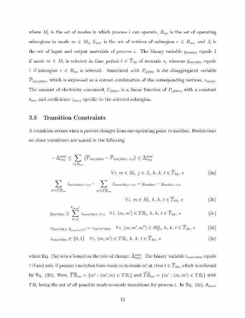
3.5 Transition Constraints

A transition occurs when a process changes from one operating point to another. Restrictions

on these transitions are stated in the following:

− ∆maximj ≤

∑r∈Rim

(P imrjhkts − P imrjhk,t−1,s

)≤ ∆max

imj

∀ i, m ∈Mi, j ∈ Ji, h, k, t ∈ T hk, s (3a)∑m′∈TRim

zim′mhk,t−1,s −∑

m′∈TRim

zimm′hk,t−1,s = yimhkts − yimhk,t−1,s

∀ i, m ∈Mi, h, k, t ∈ T hk, s (3b)

yim′hkts ≥θimm′∑t′=1

zimm′hk,t−t′,s ∀ i, (m,m′) ∈ TRi, h, k, t ∈ T hk, s (3c)

zimm′hk,t−θimm′m′′ ,s= zim′m′′hkts ∀ i, (m,m′,m′′) ∈ SQi, h, k, t ∈ T hk, s (3d)

zimm′hkts ∈ {0, 1} ∀ i, (m,m′) ∈ TRi, h, k, t ∈ T hk, s (3e)

where Eq. (3a) sets a bound on the rate of change, ∆maximj . The binary variable zimm′hkts equals

1 if and only if process i switches from modem to modem′ at time t ∈ T hk, which is enforced

by Eq. (3b). Here, TRim = {m′ : (m′,m) ∈ TRi} and TRim = {m′ : (m,m′) ∈ TRi} with

TRi being the set of all possible mode-to-mode transitions for process i. In Eq. (3c), θimm′

12

is the minimum stay time in mode m′ after switching to it from mode m, while θimm′m′′ in

Eq. (3d) is the �xed stay time in mode m′ in the chain of transitions from mode m to mode

m′ to mode m′′.

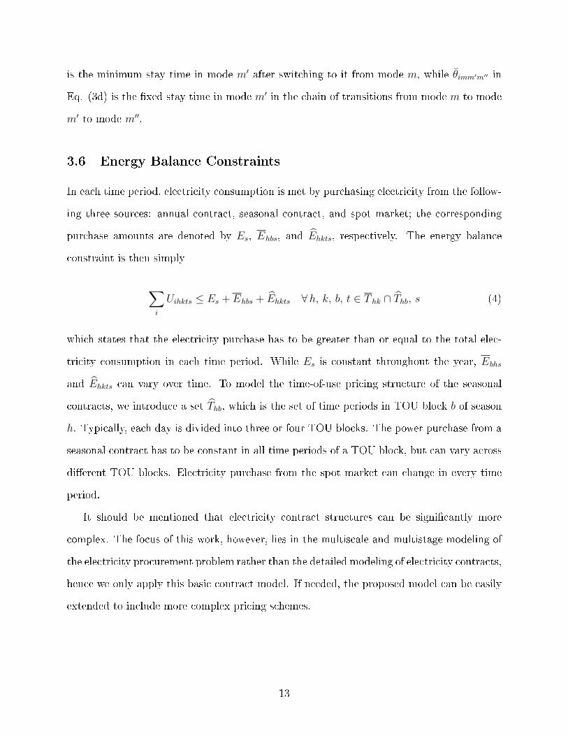
3.6 Energy Balance Constraints

In each time period, electricity consumption is met by purchasing electricity from the follow-

ing three sources: annual contract, seasonal contract, and spot market; the corresponding

purchase amounts are denoted by Es, Ehbs, and Ehkts, respectively. The energy balance

constraint is then simply

∑i

Uihkts ≤ Es + Ehbs + Ehkts ∀h, k, b, t ∈ T hk ∩ Thb, s (4)

which states that the electricity purchase has to be greater than or equal to the total elec-

tricity consumption in each time period. While Es is constant throughout the year, Ebhs

and Ehkts can vary over time. To model the time-of-use pricing structure of the seasonal

contracts, we introduce a set Thb, which is the set of time periods in TOU block b of season

h. Typically, each day is divided into three or four TOU blocks. The power purchase from a

seasonal contract has to be constant in all time periods of a TOU block, but can vary across

di�erent TOU blocks. Electricity purchase from the spot market can change in every time

period.

It should be mentioned that electricity contract structures can be signi�cantly more

complex. The focus of this work, however, lies in the multiscale and multistage modeling of

the electricity procurement problem rather than the detailed modeling of electricity contracts,

hence we only apply this basic contract model. If needed, the proposed model can be easily

extended to include more complex pricing schemes.

13

3.7 Initial Conditions

The initial state of the system is speci�ed by the following equations:

Qj,1,1,0,s = Qinij ∀ j, s (5a)

yim,1,1,0,s = yiniim ∀ i, m ∈Mi, s (5b)

zimm′,1,1,t,s = ziniimm′t ∀ i, (m,m′) ∈ TRi, −θmax

i + 1 ≤ t ≤ −1, s (5c)

which set the initial inventory levels, the initial operating modes, and the mode switching

history.

3.8 Continuity Equations

Continuity equations are required at the boundaries of each week in order to maintain con-

sistent mass balance. For Week 1 of each season, the following equations are applied to

enforce a cyclic schedule:

yimh,1,0,s = yimh,1,t1h,s ∀ i, m ∈Mi, h, s (6a)

zimm′h,1,t,s = zimm′h,1,t+t1h,s ∀ i, (m,m′) ∈ TRi, h, −θmaxi + 1 ≤ t ≤ −1, s (6b)

which state that the system at the end of the week has to be in the same state as at the

beginning of the week. We allow inventory to be accumulated during the cyclic schedule and

carried over to Week 2. According to the following equation, the excess inventory, which is

denoted by Qjhs, is de�ned as the di�erence between the inventory levels at the end and at

the beginning of Week 1 of season h:

Qjhs = Qjh,1,t1h,s−Qjh,1,0,s ∀ j, h, s (7a)

Qminjh,1,t ≤ Qjh,1,ts + (nh − 1)Qjhs ≤ Qmax

jh,1,t ∀ j, h, t ∈ T h,1, s (7b)

14

where Eq. (7b) ensures feasibility. Note that Qjhs is the only continuous variable in this

model that can take negative values.

The end of Week 1 also has to match the beginning of Week 2 of the same season, which

is enforced by the following constraints:

Qjh,1,0,s + nhQjhs = Qjh,2,0,s ∀ j, h, s (8a)

yimh,1,t1h,s = yimh,2,0,s ∀ i, m ∈Mi, h, s (8b)

zimm′h,1,t+t1h,s = zimm′h,2,t,s ∀ i, (m,m′) ∈ TRi, h, −θmaxi + 1 ≤ t ≤ −1, s. (8c)

Note that in Eq. (8a), Qjhs is multiplied by nh as the cyclic schedule is repeated nh times.

Also, recall that Week 2 does not need to have a cyclic schedule.

Finally, continuity equations are applied at the boundary between two seasons:

Qjh,2,t2h,s= Qj,h+1,1,0,s ∀ j, h ∈ H \ {h}, s (9a)

yimh,2,t2h,s = yim,h+1,1,0,s ∀ i, m ∈Mi, h ∈ H \ {h}, s (9b)

zimm′h,2,t+t2h,s = zimm′,h+1,1,t,s ∀ i, (m,m′) ∈ TRi, h ∈ H \ {h}, −θmaxi + 1 ≤ t ≤ −1, s.

(9c)

3.9 Non-Anticipativity Constraints

Following the alternative scenario tree representation shown in Figure ??, all variables are

scenario-speci�c (with index s), and all constraints have been written for each scenario in-

dividually. In order to model the multistage decision-making framework, the scenarios are

linked by non-anticipativity constraints, which equate the independent variables of scenarios

that are indistinguishable. We introduce ISh, which denotes the minimum set of indistin-

guishable scenario pairs at stage h+ 1. For example, for the set of indistinguishable scenario

{1, 2, 3, 4}, a minimum set of scenario pairs is {(1, 2), (1, 3), (1, 4)}, which has three elements.

Note that the minimum set of scenario pairs is not unique; in this example, an alternative

15

set with three elements is {(1, 2), (2, 3), (3, 4)}. By using these sets of scenario pairs, we can

write the NACs as follows:

Es = E1 ∀ s ∈ S \ {1} (10a)

Ehbs = Ehbs′ ∀h, b, (s, s′) ∈ ISh (10b)

Ehkts = Ehkts′ ∀h, k, t ∈ T hk, (s, s′) ∈ ISh (10c)

P imrjhkts = P imrjhkts′ ∀ i, m ∈Mi, r ∈ Rim, j ∈ Ji, h, k, t ∈ T hk, (s, s′) ∈ ISh (10d)

Wjhkts = Wjhkts′ ∀ j, h, k, t ∈ T hk, (s, s′) ∈ ISh (10e)

yimrhkts = yimrhkts′ ∀ i, m ∈Mi, r ∈ Rim, h, k, t ∈ T hk, (s, s′) ∈ ISh. (10f)

By taking a closer look at the problem, we notice that the di�erent stages are only

linked by the annual contract decisions and the variables connecting two consecutive seasons.

If these variables are �xed, the di�erent stages can be solved independently; hence, two

scenarios are indistinguishable at a given stage if the initial and terminal states for that

stage are the same in both scenarios. Therefore, we actually only have to consider these

variables in the NACs, i.e. Eqs. (10b)�(10f) can be replaced by the following equations:

Qjh,2,t2h,s= Qjh,2,t2h,s

′ ∀ j, h ∈ H \ {h}, (s, s′) ∈ ISh (11a)

yimh,2,t2h,s = yimh,2,t2h,s′ ∀ i, m ∈Mi, h ∈ H \ {h}, (s, s′) ∈ ISh (11b)

zimm′h,2,t+t2h,s = zimm′h,2,t+t2h,s′

∀ i, (m,m′) ∈ TRi, h ∈ H \ {h}, −θmaxi + 1 ≤ t ≤ −1, (s, s′) ∈ ISh. (11c)

By enforcing Eqs. (11), Eqs. (10b)�(10f) will be automatically satis�ed at the optimal

solution. By doing so, the number of NACs is signi�cantly reduced, which may have an

impact on the computational performance. In the remainder of the paper, we refer to Eqs.

(10) as NAC1, and to Eqs. (10a) and (11) as NAC2.

16

3.10 Objective Function

The objective is to minimize the expected total operating cost, TC, which consists of the

expected electricity cost, EC, the expected inventory cost, IC, and the expected cost of

purchasing additional products, PC:

TC = EC + IC + PC. (12)

The expected electricity cost is calculated as follows:

EC =∑s

ϕs

αEs +∑h

∑b

αhbEhbs + nh∑t∈Th,1

αh,1,t Eh,1,ts +∑t∈Th,2

αh,2,t Eh,2,ts

(13)

where ϕs is the probability of scenario s, α, αhb, and αhkt are cost coe�cients, and nh is the

number of times the cyclic schedule of season h is repeated.

The inventory cost and cost of purchasing products are

IC =∑s

ϕs∑j

∑h

βjh

nh ∑t∈Th,1

Qjh,1,ts +

nh−1∑k=1

k |T h,1|Qjhs +∑t∈Th,2

Qjh,2,ts

(14a)

PC =∑s

ϕs∑j

∑h

ψjh

nh ∑t∈Th,1

Wjh,1,ts +∑t∈Th,2

Wjh,2,ts

(14b)

where the season-dependent cost coe�cients are denoted by βjh and ψjh.

4 Value of Stochastic Solution for Multistage Problems

The value of stochastic solution (VSS)21 is commonly used as a measure for the bene�t that

one can obtain from stochastic programming when compared with deterministic optimiza-

tion. The VSS was initially developed for two-stage stochastic programming; only recently,

it has been extended to the case of multistage problems25,26. As a result, the VSS has rarely

17

been applied to multistage problems in the literature. However, computing the VSS is essen-

tial as it would otherwise be unclear whether it is worthwhile spending the e�ort on solving

a computationally more challenging stochastic program.

We adapt the procedure proposed by Escudero et al. 25 , which evaluates the VSS in

a multistage setting in a rolling horizon fashion. The problem boils down to computing

the expected result of solving the deterministic problem (using the expected values of the

uncertain parameters) at every stage. The very intuitive way to accomplish this is as follows:

starting at the root node of the scenario tree, solve the deterministic problem, �x the here-

and-now decisions for the current node, move to the next stage, solve the deterministic

problem for each node (i.e. realization of the uncertainty) at that stage, �x the here-and-

now decisions for that stage, move on to the next stage, repeat this procedure until the

�nal stage is reached, and compute the expected outcome over the set of scenarios. In the

following, we formalize this procedure and also extend it to compute the value of two-stage

stochastic solution for multistage problems.

First, to more conveniently describe the standard scenario tree, we introduce the stage

index g and the node index f . As illustrated in Figure 3, each node is uniquely mapped to

its index pair (g, f), where the numbering of the nodes starts at 1 for each stage. We further

introduce Sgf , which is the set of indistinguishable scenarios for node (g, f).

1 2 3 4

(1,1)

(2,1) (2,2)

(3,1) (3,2) (3,3) (3,4)

𝑺 𝟏,𝟏 = 𝟏, 𝟐, 𝟑, 𝟒

𝑺 𝟐,𝟏 = 𝟏, 𝟐 𝑺 𝟐,𝟐 = 𝟑, 𝟒

Figure 3: Additional notation for describing the standard scenario tree.

18

The proposed multistage stochastic programming model, denoted by (MSP), can be

formulated in the following compact form:

ZMSP = min∑s

∑g

ϕs cTg xgs

s.t.

g∑g′=1

Ag′ xg′s = dgs ∀ g, s

xgs = xgs′ ∀ g, (s, s′) ∈ ISg

xgs ∈ Xg ∀ g, s

(MSP)

where ZMSP denotes the optimal objective function value, cg is the cost vector for stage g,

Ag is the constraint matrix for the general decision variable vector xgs, dgs is the demand

(strictly speaking, this is a right-hand side vector with nonzero elements only where the

equations involve the demand) at stage g for scenario s, ISg is the set of indistinguishable

scenario pairs at stage g, and Xg is a feasibility set constructed from the corresponding

bound and integrality constraints. The multistage character of the formulation is expressed

in the �rst set of constraints, followed by the NACs.

The deterministic problem can then be formulated as follows:

ZDP = min∑g

cTg xg

s.t.

g∑g′=1

Ag′ xg′ = dg ∀ g

xg ∈ Xg ∀ g

(DP)

where only the expected demand pro�le, dg, is considered and thus we no longer require the

scenario index in the decision variable xg as well as the NACs.

The following deterministic problem is solved at a given node (g∗, f):

ZDPg∗f = (DP) s.t. xg′ = xDP

g∗fg′ ∀ g′ = 1, . . . , g∗ − 1 (DPg∗f )

19

where the parameter vector xDPg∗fg′ contains the here-and-now decisions obtained by solving

deterministic problems in previous stages. Note that ZDP = ZDP1,1 .

The total expected cost of solving a deterministic model at every stage with the realized

uncertainty at that stage is then

ZDP

=∑f∈F|G|

ϕf ZDP|G|,f . (15)

Note that at the �nal stage |G|, the scenario and node indices are identical. In general, Fg

denotes the set of nodes at stage g.

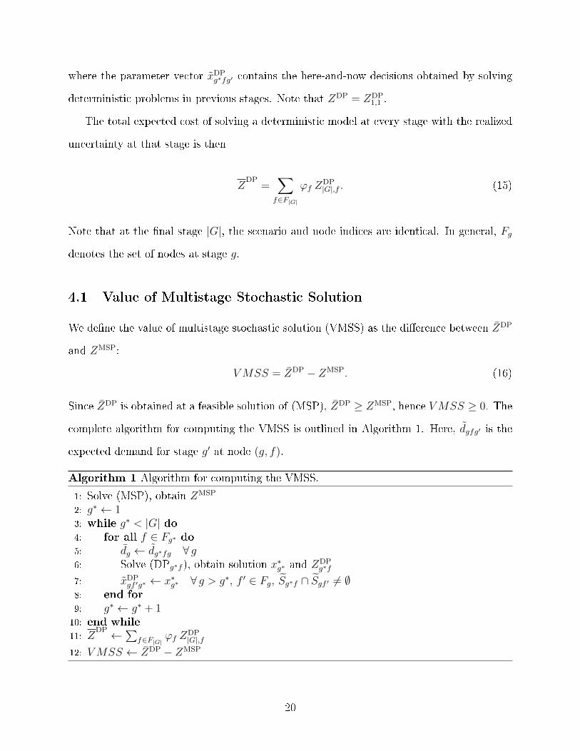
4.1 Value of Multistage Stochastic Solution

We de�ne the value of multistage stochastic solution (VMSS) as the di�erence between ZDP

and ZMSP:

VMSS = ZDP − ZMSP. (16)

Since ZDP is obtained at a feasible solution of (MSP), ZDP ≥ ZMSP, hence VMSS ≥ 0. The

complete algorithm for computing the VMSS is outlined in Algorithm 1. Here, dgfg′ is the

expected demand for stage g′ at node (g, f).

Algorithm 1 Algorithm for computing the VMSS.

1: Solve (MSP), obtain ZMSP

2: g∗ ← 13: while g∗ < |G| do4: for all f ∈ Fg∗ do5: dg ← dg∗fg ∀ g6: Solve (DPg∗f ), obtain solution x∗g∗ and Z

DPg∗f

7: xDPgf ′g∗ ← x∗g∗ ∀ g > g∗, f ′ ∈ Fg, Sg∗f ∩ Sgf ′ 6= ∅

8: end for

9: g∗ ← g∗ + 110: end while

11: ZDP ←

∑f∈F|G| ϕf Z

DP|G|,f

12: VMSS ← ZDP − ZMSP

20

4.2 Value of Two-Stage Stochastic Solution

In addition to the VMSS, we introduce the value of two-stage stochastic solution (VTSS)

for a multistage problem, which quanti�es the bene�t of using a two-stage approximation of

the multistage formulation. In a two-stage formulation, the NACs are only enforced for the

current stage. At each stage, the following problem is solved:

ZTSPg∗ = min

∑s

∑g

ϕs cTg xgs

s.t.

g∑g′=1

Ag′ xg′s = dgs ∀ g, s

xg∗s = xg∗s′ ∀ (s, s′) ∈ ISg∗

xg′s = xTSPg′s ∀ g′ = 1, . . . , g∗ − 1, s

xgs ∈ Xg ∀ g, s

(TSPg∗)

where the results from previous stages are stored in xTSPg′s . The VTSS is then de�ned as

V TSS = ZDP − ZTSP|G| . (17)

The complete algorithm for computing the VTSS is outlined in Algorithm 2. Note that

V TSS ≤ VMSS and that the VTSS can be negative.

5 Solution Method

In industrial applications, already the deterministic problem often has hundreds of thou-

sands of variables and constraints. When applying the multistage formulation with a realis-

tic number of scenarios, the numbers of variables and constraints easily go up to the tens of

millions. As a result, special algorithms are required to solve these problems in a reasonable

time. Here, we apply the progressive hedging algorithm, which decomposes the problem by

scenarios by removing the NACs. The subproblems are then solved with a modi�ed objective

21

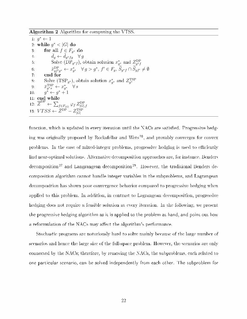
Algorithm 2 Algorithm for computing the VTSS.

1: g∗ ← 12: while g∗ < |G| do3: for all f ∈ Fg∗ do4: dg ← dg∗fg ∀ g5: Solve (DPg∗f ), obtain solution x∗g∗ and Z

DPg∗f

6: xDPgf ′g∗ ← x∗g∗ ∀ g > g∗, f ′ ∈ Fg, Sg∗f ∩ Sgf ′ 6= ∅

7: end for

8: Solve (TSPg∗), obtain solution x∗g∗ and ZTSPg∗

9: xTSPg∗s ← x∗g∗ ∀ s

10: g∗ ← g∗ + 111: end while

12: ZDP ←

∑f∈F|G| ϕf Z

DP|G|,f

13: V TSS ← ZDP − ZTSP|G|

function, which is updated in every iteration until the NACs are satis�ed. Progressive hedg-

ing was originally proposed by Rockafellar and Wets 20 , and provably converges for convex

problems. In the case of mixed-integer problems, progressive hedging is used to e�ciently

�nd near-optimal solutions. Alternative decomposition approaches are, for instance, Benders

decomposition27 and Langrangean decomposition28. However, the traditional Benders de-

composition algorithm cannot handle integer variables in the subproblems, and Lagrangean

decomposition has shown poor convergence behavior compared to progressive hedging when

applied to this problem. In addition, in contrast to Lagrangean decomposition, progressive

hedging does not require a feasible solution at every iteration. In the following, we present

the progressive hedging algorithm as it is applied to the problem at hand, and point out how

a reformulation of the NACs may a�ect the algorithm's performance.

Stochastic programs are notoriously hard to solve mainly because of the large number of

scenarios and hence the large size of the full-space problem. However, the scenarios are only

connected by the NACs; therefore, by removing the NACs, the subproblems, each related to

one particular scenario, can be solved independently from each other. The subproblem for

22

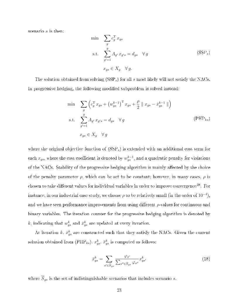
scenario s is then:

min∑g

cTg xgs

s.t.

g∑g′=1

Ag′ xg′s = dgs ∀ g

xgs ∈ Xg ∀ g.

(SSPs)

The solution obtained from solving (SSPs) for all s most likely will not satisfy the NACs.

In progressive hedging, the following modi�ed subproblem is solved instead:

min∑g

(cTg xgs +

(wk−1gs

)Txgs +

ρ

2‖ xgs − xk−1

gs ‖)

s.t.

g∑g′=1

Ag′ xg′s = dgs ∀ g

xgs ∈ Xg ∀ g

(PHPks)

where the original objective function of (SSPs) is extended with an additional cost term for

each xgs, where the cost coe�cient is denoted by wk−1gs , and a quadratic penalty for violations

of the NACs. Stability of the progressive hedging algorithm is mainly a�ected by the choice

of the penalty parameter ρ, which can be set to be constant; however, in many cases, ρ is

chosen to take di�erent values for individual variables in order to improve convergence29. For

instance, in our industrial case study, we choose ρ to be relatively small (in the order of 10−4),

and we have seen performance improvements from using di�erent ρ-values for continuous and

binary variables. The iteration counter for the progressive hedging algorithm is denoted by

k, indicating that wkgs and xkgs are updated at every iteration.

At iteration k, xkgs are constructed such that they satisfy the NACs. Given the current

solution obtained from (PHPks), xkgs, xkgs is computed as follows:

xkgs =∑s′∈Sgs

ϕs′∑s′′∈Sgs

ϕs′′xkgs′ (18)

where Sgs is the set of indistinguishable scenarios that includes scenario s.

23

The complete progressive hedging algorithm is shown in Algorithm 3. The algorithm is

initialized by solving (SSPs) for all scenarios (in parallel). Then, at every iteration k, xkgs

and wkgs are computed and the updated (PHPks) is solved for all scenarios. The algorithm

terminates when the maximum number of iterations, K, is reached or if the sum of the NAC

violations, Γk, is less than a prespeci�ed tolerance ε.

Algorithm 3 The progressive hedging algorithm.

1: k ← 02: for all s do3: Solve (SSPs), obtain solution xkgs4: end for

5: for all g, s do6: xkgs ←

∑s′∈Sgs

ϕs′∑s′′∈Sgs

ϕs′′xkgs′

7: wkgs ← ρ(xkgs − xkgs)8: end for

9: Γk ← ε+ 110: k ← k + 111: while k ≤ K and Γk−1 ≥ ε do12: for all s do13: Solve (PHPks), obtain solution xkgs14: end for

15: for all g, s do16: xkgs ←

∑s′∈Sgs

ϕs′∑s′′∈Sgs

ϕs′′xkgs′

17: wkgs ← wk−1gs + ρ(xkgs − xkgs)

18: end for

19: Γk ←∑

g

∑s ϕs ‖ xgs − xgs ‖

20: k ← k + 121: end while

We notice that it su�ces to only include the variables that are involved in the NACs in the

additional terms of the objective function since all remaining variables will be consistent with

the NACs when these are satis�ed. Thus, we conjecture that the algorithm's performance

will to a certain extent depend on the formulation of the NACs since the number of NACs is

directly related to the number of additional terms in the objective function and the number

of parameters to be updated at each iteration. Typically, the larger the number of NACs, the

longer the algorithm will take to converge and the more likely we will encounter numerical

24

issues. We demonstrate the impact of the two alternative sets of NACs, NAC1 and NAC2,

on the algorithm in Section 7.

If Γk > 0 when the algorithm terminates, the obtained solution is still not a feasible

solution to the original problem (MSP). A feasible solution is then obtained through some

heuristic, e.g. by �xing a subset of the variables to the values of xkgs (with rounded values

for binary variables).

6 Illustrative Example

The process considered in this illustrative example is represented by the process network

shown in Figure 4. Here, Process I converts A into B, which can then be separated into C

and D through Process II. The desired product is D. Each process has two operating modes,

o� and on, where each on mode is characterized by a simple range of feasible production and

a linear electricity consumption correlation (see Figure 4).

IA II

D

B

C

Figure 4: Process network for the illustrative example. The �gure shows for each processthe corresponding feasible production range and electricity consumption correlation, and foreach material the inventory capacity. The minimum stay time in the o� mode is assumed tobe 6 time periods long. The minimum inventory level for each material is zero.

We consider a planning horizon consisting of three seasons with each season being 13

weeks long. The �rst 12 weeks of each season are modeled with Week 1 (cyclic) and the last

week is modeled with Week 2 (noncyclic). Each week consists of 42 time periods where one

25

time period is four hours long. At the beginning of the planning horizon, both processes are

in the on mode, and 2000 kg of initial inventory is available for each of B and D.

The given process is assumed to produce a high-margin product; hence, while the feed

A can be purchased at a cost of $ 0.2/kg, the purchasing costs for the intermediate and

�nal products are very high, namely $ 10/kg for B and $ 20/kg for D. With $ 0.005/kg and

$ 0.07/kg per time period, the inventory costs for B and D are also relatively high. It is

assumed that the waste product C is disposed at no cost.

Demand is assumed to be uncertain but constant over the course of each season. The

nominal demands per time period in the three seasons are 750 kg, 700 kg, and 800 kg, respec-

tively. We approximate the demand distribution with two realizations for the demand in

each season, one taking the value of the nominal demand multiplied by 1− ξ and the other

being 1 + ξ times the nominal demand, which results in eight scenarios of equal probability

(0.125). For this case study, we consider the following three cases:

• Case 1: low level of uncertainty, ξ = 0.05

• Case 2: medium level of uncertainty, ξ = 0.1

• Case 3: high level of uncertainty, ξ = 0.2

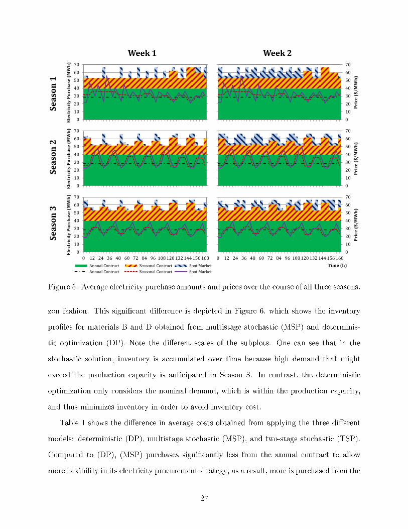
We take a detailed look at the results obtained from solving the multistage stochastic

model (MSP) for Case 3, the case with the highest level of uncertainty. The electricity

procurement schedule is depicted in Figure 5, which shows the average amounts of electricity

purchased from the three di�erent sources over time and the corresponding price pro�les.

Because of its low price, the majority of the consumed electricity is purchased from the annual

contract. Signi�cant amounts are also purchased from the seasonal contracts and from the

spot market; here, the solution clearly suggests avoiding high-price hours by leveraging the

�exibility in the production process.

The solution also suggests making use of the inventory to hedge against the uncertainty

in demand, which is not considered when solving the deterministic model in a rolling hori-

26

0

10

20

30

40

50

60

70

0

10

20

30

40

50

60

70

0 12 24 36 48 60 72 84 96 108 120 132 144 156 168

Ele

ctri

city

Pu

rch

ase

(M

Wh

)

Annual Contract Seasonal Contract Spot Market

Annual Contract Seasonal Contract Spot Market

0

10

20

30

40

50

60

70

0

10

20

30

40

50

60

70

0 12 24 36 48 60 72 84 96 108 120 132 144 156 168

Pri

ce (

$/

MW

h)

Time (h)

Week 1

0

10

20

30

40

50

60

70

0

10

20

30

40

50

60

70

0 12 24 36 48 60 72 84 96 108 120 132 144 156 168

Ele

ctri

city

Pu

rch

ase

(M

Wh

)

0

10

20

30

40

50

60

70

0

10

20

30

40

50

60

70

0 12 24 36 48 60 72 84 96 108 120 132 144 156 168

Pri

ce (

$/

MW

h)

0

10

20

30

40

50

60

70

0

10

20

30

40

50

60

70

0 12 24 36 48 60 72 84 96 108 120 132 144 156 168

Pri

ce (

$/

MW

h)

0

10

20

30

40

50

60

70

0

10

20

30

40

50

60

70

0 12 24 36 48 60 72 84 96 108 120 132 144 156 168

Ele

ctri

city

Pu

rch

ase

(M

Wh

)

Week 2 S

ea

son

1

Se

aso

n 2

S

ea

son

3

Figure 5: Average electricity purchase amounts and prices over the course of all three seasons.

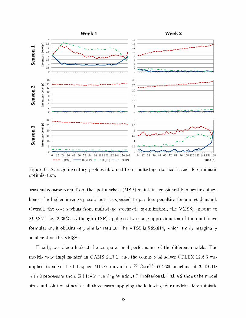
zon fashion. This signi�cant di�erence is depicted in Figure 6, which shows the inventory

pro�les for materials B and D obtained from multistage stochastic (MSP) and determinis-

tic optimization (DP). Note the di�erent scales of the subplots. One can see that in the

stochastic solution, inventory is accumulated over time because high demand that might

exceed the production capacity is anticipated in Season 3. In contrast, the deterministic

optimization only considers the nominal demand, which is within the production capacity,

and thus minimizes inventory in order to avoid inventory cost.

Table 1 shows the di�erence in average costs obtained from applying the three di�erent

models: deterministic (DP), multistage stochastic (MSP), and two-stage stochastic (TSP).

Compared to (DP), (MSP) purchases signi�cantly less from the annual contract to allow

more �exibility in its electricity procurement strategy; as a result, more is purchased from the

27

0

0.5

1

1.5

2

2.5

3

3.5

4

0 12 24 36 48 60 72 84 96 108 120 132 144 156 168

Inv

en

tory

Le

ve

l (t

)

0

2

4

6

8

10

12

14

16

0 12 24 36 48 60 72 84 96 108 120 132 144 156 168

0

2

4

6

8

10

12

14

16

0 12 24 36 48 60 72 84 96 108 120 132 144 156 168

Inv

en

tory

Le

ve

l (t

)

0

5

10

15

20

25

30

0 12 24 36 48 60 72 84 96 108 120 132 144 156 168

0

5

10

15

20

25

30

0 12 24 36 48 60 72 84 96 108 120 132 144 156 168

Inv

en

tory

Le

ve

l (t

)

B (MSP) D (MSP) B (DP) D (DP)

0

0.5

1

1.5

2

2.5

3

0 12 24 36 48 60 72 84 96 108 120 132 144 156 168

Time (h)

Week 1 S

ea

son

1

Week 2 S

ea

son

2

Se

aso

n 3

Figure 6: Average inventory pro�les obtained from multistage stochastic and deterministicoptimization.

seasonal contracts and from the spot market. (MSP) maintains considerably more inventory,

hence the higher inventory cost, but is expected to pay less penalties for unmet demand.

Overall, the cost savings from multistage stochastic optimization, the VMSS, amount to

$ 99,851, i.e. 2.36%. Although (TSP) applies a two-stage approximation of the multistage

formulation, it obtains very similar results. The VTSS is $ 99,814, which is only marginally

smaller than the VMSS.

Finally, we take a look at the computational performance of the di�erent models. The

models were implemented in GAMS 24.7.1, and the commercial solver CPLEX 12.6.3 was

applied to solve the full-space MILPs on an Intel R© CoreTM i7-2600 machine at 3.40GHz

with 8 processors and 8GB RAM running Windows 7 Professional. Table 2 shows the model

sizes and solution times for all three cases, applying the following four models: deterministic

28

Table 1: Average costs for Case 3 of the illustrative example.

(DP) (MSP) (TSP)

Cost Annual Contract ($) 2,217,688 1,839,642 1,877,101Cost Seasonal Contracts ($) 449,507 744,837 712,291

Cost Spot Market ($) 29,786 110,859 106,086Inventory Cost ($) 33,804 131,770 131,520

Product Purchasing Cost ($) 1,503,581 1,307,406 1,307,554Total Cost ($) 4,234,366 4,134,515 4,134,552

(DP), multistage with the original set of NACs (MSP-NAC1), multistage with alternative set

of NACs (MSP-NAC2), as described in Section 3.9, and two-stage (TSP). All models were

solved to optimality. One can see that in this particular case, solution times increase with the

level of uncertainty. Naturally, due to the larger number of scenarios, the stochastic models

are signi�cantly larger than the deterministic model and require more time to solve. The

interesting observation is that although (MSP-NAC1) is larger in size than (MSP-NAC2), it

requires less time to solve, and also less than (TSP), which may be because (MSP-NAC1)

is more tightly constrained. This is just another example for the fact that in mixed-integer

programming, smaller model sizes do not necessarily lead to shorter solution times. However,

the situation may change when we solve larger instances with the proposed solution algorithm

(see Section 7).

Table 2: Model sizes and solution times for the illustrative example.

(DP) (MSP-NAC1) (MSP-NAC2) (TSP)

# of Bin. Variables 3,168 25,344 25,344 25,344# of Cont. Variables 7,634 61,044 61,044 61,044# of Constraints 10,456 98,887 83,917 83,627

Solution Time Case 1 (s) 1.6 25 132 226Solution Time Case 2 (s) 1.6 69 284 452Solution Time Case 3 (s) 1.9 134 867 533

29

7 Industrial Case Study

We now apply the proposed framework to a real-world industrial case study provided by

Praxair. Here, we consider the air separation site represented by the process network in

Figure 2, which is described in Section 3.3. Note that due to con�dentiality reasons, we

cannot disclose information about the plant speci�cations as well as the actual product

demand. Therefore, all results presented in this section are given without units and the

values are normalized if necessary.

The planning horizon of one year is divided into four seasons (winter, spring, summer, and

fall), where each season is represented by one week with a cyclic schedule. We do not consider

a second noncyclic week because the inventory cost is negligibly small, i.e. an abrupt change

in inventory within one week is unlikely to have a signi�cant bene�t. Therefore, introducing

a second week for each season would only unnecessarily increase the size of the model. An

hourly time discretization is applied, resulting in 168 time periods per week.

The electricity prices for each season are based on price data from 2013 to 2015 made

available by the independent system operator ERCOT, which manages the Texas Intercon-

nection.

For each season, we consider three possible demand realizations, resulting in 81 scenarios

in total. The problem is solved for three di�erent cases:

• Case 1 with low level of uncertainty (± 5 %)

• Case 2 with high level of uncertainty (± 20 %)

• Case 3 with the same demand scenarios as in Case 2, but with the nitrogen lique�er

being unavailable throughout the year

Because of the size of the multistage problem, solving it in full space is intractable. There-

fore, we perform a computational study in order to determine, among the given alternatives,

the best formulation and algorithm for e�ectively solving this large-scale problem. To avoid

30

memory issues and to increase the capacity of solving the subproblems in the progressive

hedging algorithm in parallel, we solved all models from the industrial case study on an

Intel R© Xenon R© machine at 2.6GHz with 24 cores and 64GB RAM.

The full-space model with the original set of NACs (MSP-NAC1) has 7,139,103 contin-

uous variables, 2,586,168 binary variables, and 11,310,434 constraints including 2,367,704

NACs. In contrast, (MSP-NAC2) only has 60,464 NACs. In Table 3, we show the optimal-

ity gaps and objective function values obtained from solving the full-space model with the

two di�erent sets of NACs for the three cases. For each instance, the solution time limit

is set to 10 hours. From the results, it is obvious that solving the problem in full space is

computationally intractable. In none of the instances, a lower bound can be obtained within

the solution time limit, hence no optimality gap can be computed. The feasible solutions

are obtained from primal heuristics, but result in very high objective function values.

Table 3: Computational results for solving the full-space model (MSP).

Case 1 Case 2 Case 3

NAC1 NAC2 NAC1 NAC2 NAC1 NAC2

Solution Time (s) 36,000 36,000 36,000 36,000 36,000 36,000Optimality Gap (%) n/a n/a n/a n/a n/a n/a

Objective Function Value 15,367 15,289 15,522 15,443 13,216 13,153

Table 4 shows the performance of the proposed progressive hedging algorithm with the

two di�erent sets of NACs is shown. The algorithm is set up such that the solution of each

subproblem terminates when an optimality gap of 0.1% or the time limit of 10 minutes is

reached. The limit on the number of iterations is set to 10. In all instances, the number

of iterations limit is reached, resulting in similar solution times, in average about 4.5 hours.

Despite similar solution times and same number of iterations, one can see that consistently

across all cases, solutions with lower objective function values are achieved by the NAC2

formulation. The di�erences may seem small but are in fact very signi�cant; while the NAC2

solutions show a bene�t of stochastic optimization compared with deterministic optimization,

31

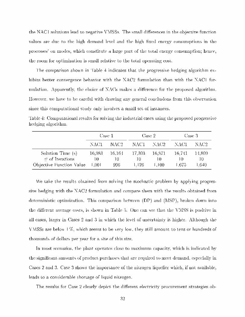
the NAC1 solutions lead to negative VMSSs. The small di�erences in the objective function

values are due to the high demand level and the high �xed energy consumptions in the

processes' on modes, which constitute a large part of the total energy consumption; hence,

the room for optimization is small relative to the total operating cost.

The comparison shown in Table 4 indicates that the progressive hedging algorithm ex-

hibits better convergence behavior with the NAC2 formulation than with the NAC1 for-

mulation. Apparently, the choice of NACs makes a di�erence for the proposed algorithm.

However, we have to be careful with drawing any general conclusions from this observation

since this computational study only involves a small set of instances.

Table 4: Computational results for solving the industrial cases using the proposed progressivehedging algorithm.

Case 1 Case 2 Case 3

NAC1 NAC2 NAC1 NAC2 NAC1 NAC2

Solution Time (s) 16,983 16,164 17,303 16,871 16,741 14,809# of Iterations 10 10 10 10 10 10

Objective Function Value 1,001 996 1,126 1,100 1,675 1,640

We take the results obtained from solving the stochastic problem by applying progres-

sive hedging with the NAC2 formulation and compare them with the results obtained from

deterministic optimization. This comparison between (DP) and (MSP), broken down into

the di�erent average costs, is shown in Table 5. One can see that the VMSS is positive in

all cases, larger in Cases 2 and 3 in which the level of uncertainty is higher. Although the

VMSSs are below 1%, which seems to be very low, they still amount to tens or hundreds of

thousands of dollars per year for a site of this size.

In most scenarios, the plant operates close to maximum capacity, which is indicated by

the signi�cant amounts of product purchases that are required to meet demand, especially in

Cases 2 and 3. Case 3 shows the importance of the nitrogen lique�er which, if not available,

leads to a considerable shortage of liquid nitrogen.

The results for Case 2 clearly depict the di�erent electricity procurement strategies ob-

32

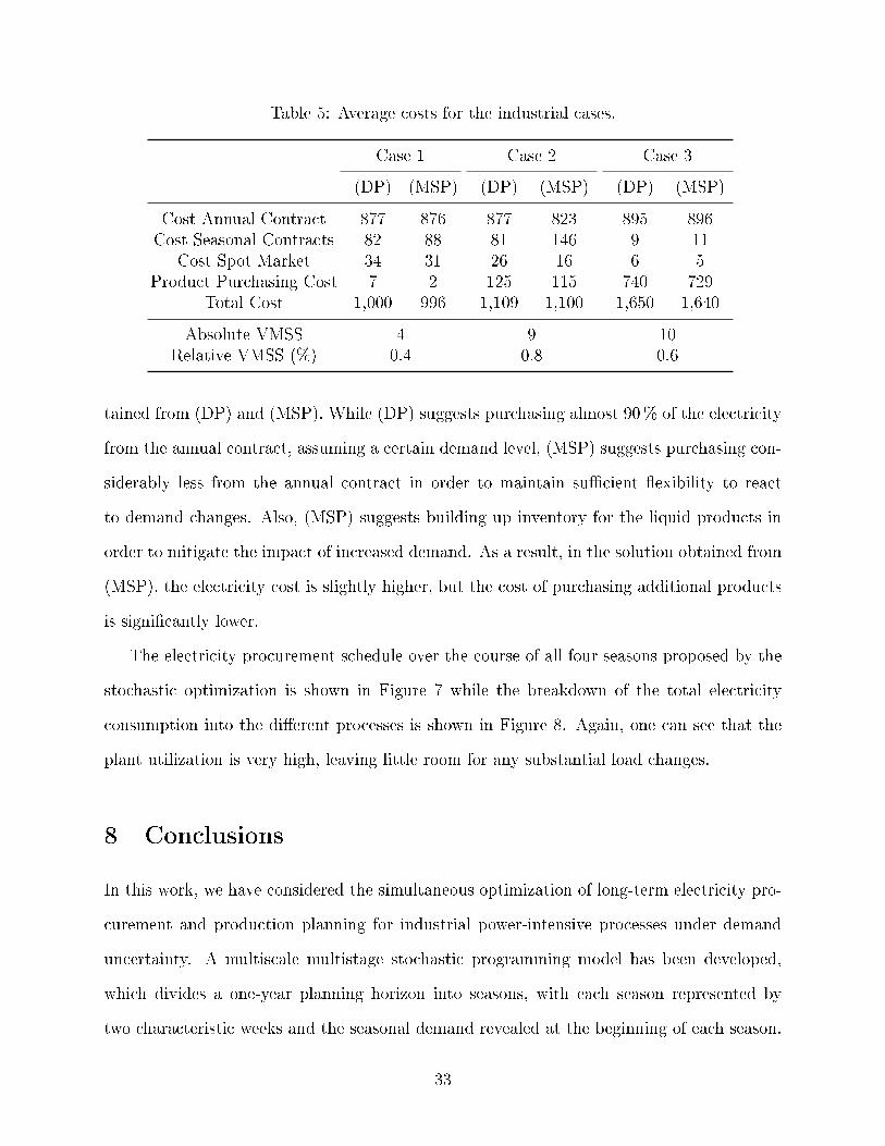
Table 5: Average costs for the industrial cases.

Case 1 Case 2 Case 3

(DP) (MSP) (DP) (MSP) (DP) (MSP)

Cost Annual Contract 877 876 877 823 895 896Cost Seasonal Contracts 82 88 81 146 9 11

Cost Spot Market 34 31 26 16 6 5Product Purchasing Cost 7 2 125 115 740 729

Total Cost 1,000 996 1,109 1,100 1,650 1,640

Absolute VMSS 4 9 10Relative VMSS (%) 0.4 0.8 0.6

tained from (DP) and (MSP). While (DP) suggests purchasing almost 90% of the electricity

from the annual contract, assuming a certain demand level, (MSP) suggests purchasing con-

siderably less from the annual contract in order to maintain su�cient �exibility to react

to demand changes. Also, (MSP) suggests building up inventory for the liquid products in

order to mitigate the impact of increased demand. As a result, in the solution obtained from

(MSP), the electricity cost is slightly higher, but the cost of purchasing additional products

is signi�cantly lower.

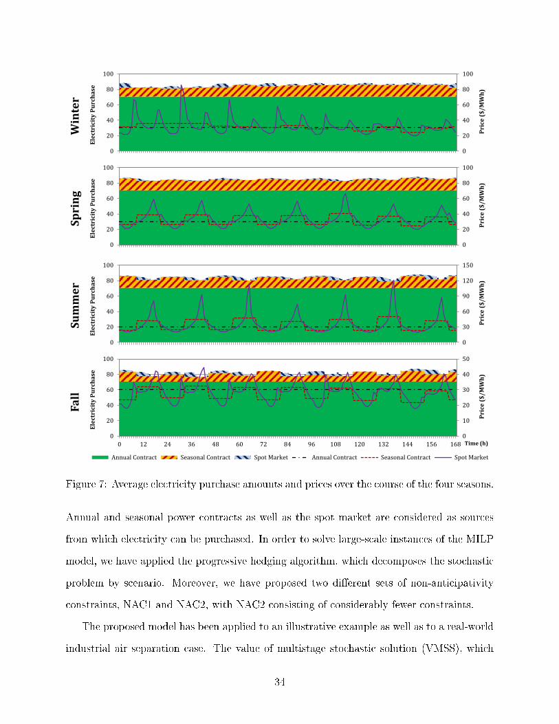
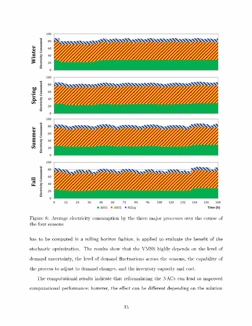
The electricity procurement schedule over the course of all four seasons proposed by the

stochastic optimization is shown in Figure 7 while the breakdown of the total electricity

consumption into the di�erent processes is shown in Figure 8. Again, one can see that the

plant utilization is very high, leaving little room for any substantial load changes.

8 Conclusions

In this work, we have considered the simultaneous optimization of long-term electricity pro-

curement and production planning for industrial power-intensive processes under demand

uncertainty. A multiscale multistage stochastic programming model has been developed,

which divides a one-year planning horizon into seasons, with each season represented by

two characteristic weeks and the seasonal demand revealed at the beginning of each season.

33

0

20

40

60

80

100

0

20

40

60

80

100

0 12 24 36 48 60 72 84 96 108 120 132 144 156 168

Pric

e ($

/MW

h)

Elec

tric

ity

Purc

hase

Time (h)

0

20

40

60

80

100

0

20

40

60

80

100

0 12 24 36 48 60 72 84 96 108 120 132 144 156 168

Pric

e ($

/MW

h)

Elec

tric

ity

Purc

hase

Time (h)

0

30

60

90

120

150

0

20

40

60

80

100

0 12 24 36 48 60 72 84 96 108 120 132 144 156 168

Pric

e ($

/MW

h)

Elec

tric

ity

Purc

hase

Time (h)

0

10

20

30

40

50

0

20

40

60

80

100

0 12 24 36 48 60 72 84 96 108 120 132 144 156 168

Pric

e ($

/MW

h)

Elec

tric

ity

Purc

hase

Time (h)

Annual Contract Seasonal Contract Spot Market Annual Contract Seasonal Contract Spot Market

Spri

ng

Sum

mer

Fa

ll W

inte

r

Figure 7: Average electricity purchase amounts and prices over the course of the four seasons.

Annual and seasonal power contracts as well as the spot market are considered as sources

from which electricity can be purchased. In order to solve large-scale instances of the MILP

model, we have applied the progressive hedging algorithm, which decomposes the stochastic

problem by scenario. Moreover, we have proposed two di�erent sets of non-anticipativity

constraints, NAC1 and NAC2, with NAC2 consisting of considerably fewer constraints.

The proposed model has been applied to an illustrative example as well as to a real-world

industrial air separation case. The value of multistage stochastic solution (VMSS), which

34

0

20

40

60

80

100

0 12 24 36 48 60 72 84 96 108 120 132 144 156 168

Elec

tric

ity

Cons

umed

Time (h)

0

20

40

60

80

100

0 12 24 36 48 60 72 84 96 108 120 132 144 156 168

Elec

tric

ity

Cons

umed

Time (h)

0

20

40

60

80

100

0 12 24 36 48 60 72 84 96 108 120 132 144 156 168

Elec

tric

ity

Cons

umed

Time (h)

0

20

40

60

80

100

0 12 24 36 48 60 72 84 96 108 120 132 144 156 168

Elec

tric

ity

Cons

umed

Time (h) ASU1 ASU2 N2Liq

Spri

ng

Sum

mer

Fa

ll W

inte

r

Figure 8: Average electricity consumption by the three major processes over the course ofthe four seasons.

has to be computed in a rolling horizon fashion, is applied to evaluate the bene�t of the

stochastic optimization. The results show that the VMSS highly depends on the level of

demand uncertainty, the level of demand �uctuations across the seasons, the capability of

the process to adjust to demand changes, and the inventory capacity and cost.

The computational results indicate that reformulating the NACs can lead to improved

computational performance; however, the e�ect can be di�erent depending on the solution

35

strategy. In our case, when solving the medium-size problems with the full-space model, the

NAC1 formulation is computationally more e�cient. In contrast, when solving the large-

scale problems using progressive hedging, the NAC2 formulation exhibits a notably better

convergence behavior.

Nomenclature

Indices

b time-of-use blocks

h seasons

i processes

j materials

k weeks

l vertices

m,m′,m′′ operating modes

r operating subregions

s scenarios

t time periods

Sets

H seasons

I processes

Ij processes producing material j

Ij processes receiving material j

ISh minimum set of indistinguishable scenario pairs at stage h+ 1

Ji input and output materials of process i

36

K weeks

Mi operating modes of process i

Rim operating subregions in mode m of process i

S scenarios

SQi prede�ned sequences of mode transitions in process i

Thk time periods of week k in season h

T hk time periods in the scheduling horizon of week k in season h

Thb time periods in time-of-use block b of season h

TRi possible mode transitions in process i

TRim modes of process i from which mode m can be directly reached

TRim modes of process i which can be directly reached from mode m

Parameters

Djhkts demand for material j in time period t of week k in season h in scenario s (kg)

h last season

nh number of times the cyclic schedule of season h is repeated

Qinij initial inventory of material j (kg)

Qminjhkt minimum inventory level for material j in time period t of week k in season h (kg)

Qmaxjhkt maximum inventory level for material j in time period t of week k in season h (kg)

Wmaxjhkt maximum amount of material j that can be purchased in time period t of week k

in season h (kg)

tkh last time period in the set of time periods T hk

vimrlj amount of material j produced in one time period at vertex l of subregion r

in mode m of process i (kg)

yiniim 1 if process i was operating in mode m in the time period before the start of the

planning horizon

ziniimm′t 1 if operation switched from mode m to mode m′ in process i at time t before

37

the start of the planning horizon

α unit cost of purchasing electricity from the annual contract ($/kWh)

αhb unit cost of purchasing electricity in time-of-use block b from seasonal contract h ($/kWh)

αhkt unit cost of purchasing electricity in time period t of week k in season h from

the spot market ($/kWh)

βjh unit cost of storing material j in season h ($/kg)

ψjh unit cost of purchasing material j in season h ($/kg)

γimrj unit electricity consumption corresponding to material j if process i operates

in subregion r of mode m (kWh/kg)

δimr �xed electricity consumption if process i operates in subregion r of mode m (kWh)

∆t length of one time period (h)

∆maximj maximum rate of change for production of material j in mode m of process i (kg)

θimm′ minimum stay time in mode m′ after switching from mode m to m′ in process i (∆t)

θimm′m′′ �xed stay time in mode m′ of the prede�ned sequence (m,m′,m′′) in process i (∆t)

θmax maximum minimum or prede�ned stay time in a mode (∆t)

ϕs probability of scenario s

Nonnegative Continuous Variables

Es electricity purchased from the annual contract in scenario s (kWh)

Ehbs electricity purchased in time-of-use block b from seasonal contract h in scenario s (kWh)

Ehkts electricity purchased from the spot market time period t of week k in season h

in scenario s (kWh)

EC expected electricity cost ($)

IC expected inventory cost ($)

Pijhkts amount of material j consumed or produced by process i in time period t of week k

in season h in scenario s (kg)

P imrjhkts amount of material j consumed or produced in subregion r of mode m of process i

38

in time period t of week k in season h in scenario s (kg)

PC expected cost of purchasing additional products ($)

Qjhkts inventory level for material j at time t in week k of season h in scenario s (kg)

TC total expected operating cost ($)

Wjhkts amount of material j purchased in time period t of week k in season h in scenario s (kg)

λimrlhkts coe�cient for vertex l of subregion r in mode m of process i in time period t

of week k in season h in scenario s

Uihkts electricity consumed by process i in time period t of week k in season h in scenario s (kWh)

Unrestricted Continuous Variables

Qjhs di�erence between the inventory levels at the end and at the beginning of Week 1

of season h in scenario s (kg)

Binary Variables

yimhkts 1 if process i operates in mode m in time period t of week k in season h in scenario s

yimrkhts 1 if process i operates in subregion r of mode m in time period t of week k in season h

in scenario s

zimm′hkts 1 if process i switches from mode m to mode m′ at time t of week k in season h

in scenario s

Acronyms

ASU air separation unit

CRS Convex Region Surrogate

CVaR conditional value-at-risk

DSM demand side management

39

MILP mixed-integer linear programming

NAC non-anticipativity constraint

TOU time-of-use

VMSS value of multistage stochastic solution

VSS value of stochastic solution

VTSS value of two-stage stochastic solution

Acknowledgement

The authors gratefully acknowledge the �nancial support from the National Science Foun-

dation under Grant CBET 1159443 and from Praxair.

References

(1) Conejo, A. J.; García-Bertrand, R.; Carrión, M.; Caballero, Á.; de Andrés, A. Optimal

Involvement in Futures Markets of a Power Producer. IEEE Transactions on Power

Systems 2008, 23, 703�711.

(2) Lima, R. M.; Novais, A. Q.; Conejo, A. J. Weekly self-scheduling, forward contract-

ing, and pool involvement for an electricity producer. An adaptive robust optimization

approach. European Journal of Operational Research 2015, 240, 457�475.

(3) Carrión, M.; Conejo, A. J.; Arroyo, J. M. Forward Contracting and Selling Price Deter-

mination for a Retailer. IEEE Transactions on Power Systems 2007, 22, 2105�2114.

(4) Hatami, A. R.; Sei�, H.; Sheikh-El-Eslami, M. K. Optimal selling price and energy

procurement strategies for a retailer in an electricity market. Electric Power Systems

Research 2009, 79, 246�254.

(5) Conejo, A. J.; Fernández-González, J. J.; Alguacil, N. Energy procurement for large

40

consumers in electricity markets. IEE Proceedings-Generation, Transmission and Dis-

tribution 2005, 152, 357�364.

(6) Conejo, A. J.; Carrión, M. Risk-constrained electricity procurement for a large con-

sumer. IEE Proceedings - Generation, Transmission and Distribution 2006, 153, 407.

(7) Carrión, M.; Philpott, A. B.; Conejo, A. J.; Arroyo, J. M. A Stochastic Programming

Approach to Electric Energy Procurement for Large Consumers. IEEE Transactions

on Power Systems 2007, 22, 744�754.

(8) Zare, K.; Moghaddam, M. P.; Sheikh El Eslami, M. K. Electricity procurement for

large consumers based on Information Gap Decision Theory. Energy Policy 2010, 38,

234�242.

(9) Beraldi, P.; Violi, A.; Scordino, N.; Sorrentino, N. Short-term electricity procurement:

A rolling horizon stochastic programming approach. Applied Mathematical Modelling

2011, 35, 3980�3990.

(10) Beraldi, P.; Violi, A.; Carrozzino, G.; Bruni, M. E. The optimal electric energy pro-

curement problem under reliability constraints. Energy Procedia 2017, 136, 283�289.

(11) Zhang, Q.; Grossmann, I. E. Enterprise-wide optimization for industrial demand side

management: Fundamentals, advances, and perspectives. Chemical Engineering Re-

search and Design 2016, 116, 114�131.

(12) Zhang, Q.; Sundaramoorthy, A.; Grossmann, I. E.; Pinto, J. M. A discrete-time schedul-

ing model for continuous power-intensive process networks with various power contracts.

Computers & Chemical Engineering 2016, 84, 382�393.

(13) Hadera, H.; Labrik, R.; Sand, G.; Engell, S.; Harjunkoski, I. An Improved Energy-

Awareness Formulation for General Precedence Continuous-Time Scheduling Models.

Industrial and Engineering Chemistry Research 2016, 55, 1336�1346.

41

(14) Zhang, Q.; Cremer, J. L.; Grossmann, I. E.; Sundaramoorthy, A.; Pinto, J. M. Risk-

based integrated production scheduling and electricity procurement for continuous

power-intensive processes. Computers & Chemical Engineering 2016, 86, 90�105.

(15) Vujanic, R.; Mariéthos, S.; Goulart, P.; Morari, M. Robust Integer Optimization and

Scheduling Problems for Large Electricity Consumers. Proceedings of the 2012 Ameri-

can Control Conference. 2012; pp 3108�3113.

(16) Zhang, Q.; Grossmann, I. E.; Heuberger, C. F.; Sundaramoorthy, A.; Pinto, J. M. Air

Separation with Cryogenic Energy Storage: Optimal Scheduling Considering Electric

Energy and Reserve Markets. AIChE Journal 2015, 61, 1547�1558.

(17) Zhang, Q.; Morari, M. F.; Grossmann, I. E.; Sundaramoorthy, A.; Pinto, J. M. An ad-

justable robust optimization approach to scheduling of continuous industrial processes

providing interruptible load. Computers & Chemical Engineering 2016, 86, 106�119.

(18) Mitra, S.; Pinto, J. M.; Grossmann, I. E. Optimal multi-scale capacity planning for

power-intensive continuous processes under time-sensitive electricity prices and demand

uncertainty. Part I: Modeling. Computers & Chemical Engineering 2014, 65, 89�101.

(19) Zhang, Q.; Sundaramoorthy, A.; Grossmann, I. E.; Pinto, J. M. Multiscale production

routing in multicommodity supply chains with complex production facilities. Computers

& Operations Research 2017, 79, 207�222.

(20) Rockafellar, R.; Wets, R. J. B. Scenarios and Policy Aggregation in Optimization under

Uncertainty. Mathematics of Operations Research 1991, 16, 119�147.

(21) Birge, J. R.; Louveaux, F. Introduction to Stochastic Programming, 2nd ed.; Springer

Science+Business Media, 2011.

(22) Apap, R. M.; Grossmann, I. E. Models and Computational Strategies for Multistage

42

Stochastic Programming under Endogenous and Exogenous Uncertainties. Computers

& Chemical Engineering 2017, 103, 233�274.

(23) Ruszczy«ski, A. Decomposition methods in stochastic programming.Mathematical Pro-

gramming 1997, 79, 333�353.

(24) Zhang, Q.; Grossmann, I. E.; Sundaramoorthy, A.; Pinto, J. M. Data-driven construc-

tion of Convex Region Surrogate models. Optimization and Engineering 2016, 17,

289�332.

(25) Escudero, L. F.; Garín, A.; María, M.; Pérez, G. The value of the stochastic solution

in multistage problems. Top 2007, 15, 48�64.

(26) Maggioni, F.; Allevi, E.; Bertocchi, M. Measures of information in multi-stage stochastic

programming. Stochastic Programming E-Print Series 2012, 1�27.

(27) Benders, J. F. Partitioning procedures for solving mixed-variables programming prob-

lems. Numerische Mathematik 1962, 4, 238�252.

(28) Geo�rion, A. M. Lagrangean Relaxation for Integer Programming. Mathematical Pro-

gramming Study 2 1974, 2, 82�114.

(29) Watson, J. P.; Woodru�, D. L. Progressive hedging innovations for a class of stochastic

mixed-integer resource allocation problems. Computational Management Science 2011,

8, 355�370.

43