Capacity planning with competitive decision-makers:Trilevel MILP formulation and solution approaches

Carlos Florensa Campoa, Pablo Garcia-Herrerosa, Pratik Misrab, ErdemArslanb, Sanjay Mehtab, Ignacio E. Grossmanna,∗

aDepartment of Chemical Engineering, Carnegie Mellon University, Pittsburgh, USA5

bAir Products and Chemicals, Inc. Allentown, USA

Abstract

Capacity planning addresses the decision problem of an industrial producerinvesting on infrastructure to satisfy future demand with the highest profit.Traditional formulations neglect the rational behavior of some external decision-10

makers by assuming either static competition or captive markets. We propose amathematical programming formulation with three levels of decision-makers tocapture the dynamics of duopolistic markets. The trilevel model is transformedinto a bilevel optimization problem with mixed-integer variables in both levelsby replacing the third-level linear program with its optimality conditions. We15

introduce new definitions required for the analysis of degeneracy in multilevelproblems, and develop two novel algorithms to solve these challenging problems.Each algorithm is shown to converge to a different type of degenerate solution.The computational experiments for capacity expansion in industrial gas marketsshow that no algorithm is strictly superior in terms of performance.20

Keywords: Multilevel programming, degeneracy, capacity expansion,competitive markets.

1. Introduction

Industrial and manufacturing companies rely on capacity expansion modelsto plan the investments that allow them to satisfy future demands. In this sector,25

the proximity of producers to customers increases supply reliability and reducestransportation costs, which provides a key competitive advantage [22, 7]. Thisfeature makes location and capacity planning a major strategic decision thatimpacts the market share obtained in an environment with rational customers.In this article, we study the case of two companies competing for the same30

market in a hierarchical framework, where the leading company first performsits capacity expansions, then the competition reacts with its own, and finallyan inelastic market observes all available capacities and minimizes its total costof supply. This is a common situation in the market of industrial gases, whichhas been the motivation for our research; we apply our model and algorithms35

to case studies from the air separation industry.The purpose of this paper is threefold: to introduce a new model based

on a trilevel mathematical programming formulation, to elaborate on the char-acteristics of general trilevel optimization problems, and to propose two novel

∗Corresponding authorEmail address: grossmann@cmu.edu (Ignacio E. Grossmann )

Preprint submitted to European Journal of Operational Research October 14, 2016

algorithms exploiting the problem structure. The remaining part of this sec-40

tion, presents a literature review of the available hierarchical capacity planningmodels, of general multilevel programs, and of the advances in algorithms tosolve them; each part specifies our contribution to the corresponding body ofwork.

1.1. Industrial capacity planning45

Capacity planning is a widely studied problem in areas requiring large cap-ital investments whose feasibility, effectiveness, and profitability can only beassessed in a long time horizon. Some examples are electrical power supply [31],communication networks [8], and Enterprise-Wide Optimization [17]. Whendealing with industrial expansions, a considerable difficulty that arises is the50

discrete nature of the decisions, as it is only possible to build new plants or pro-duction lines of a specific size. If we are additionally interested in developing arobust expansion plan that anticipates the rational reaction of the competitorsand potential costumers, it is necessary to adopt a game theoretic approach.

A foundational model in the location literature is the discrete (r|p)-centroid55

problem. It investigates what are the best locations in a network for the leadingcompany to place p new facilities, knowing that the competitors will react bychoosing r other locations [19]. There has been many applications of sequentialcompetitive location on networks [25]. Recent advances to solve this probleminclude branch-and-cut procedures [33] or exact iterative local search methods60

[1]. Nevertheless, these models do not include the cost of expansion, mainte-nance or production, and the strategies do not contemplate any time-horizon.These assumptions, that greatly simplify the problem, are not considered in ourmodel. We also allow the number of expansions to be a variable in the opti-mization problems solved by the leader and by the follower, instead of being65

predefined. Furthermore, most of the models available in the literature onlyconsider uncapacitated facilities; therefore, costumers can always be served bytheir prefered facility without considering the influence of other costumers [22].

The work presented by Karakitsiou and Migdalas [23] recognizes the fail-ure to capture a rational market in previous models. They propose a more70

realistic model using Nash equilibrium and a demand curve that is assignedto the costumers. In their model, only the leader expands and all competitorshave fixed capacity; they only compete by deciding their production quantities.Models with similar characteristics have already been proposed [35] and ex-tensions also consider shipping dynamics or multi-period time horizon [14, 28].75

These Stackelberg-Nash-Cournot formulations usually yield Equilibrium Prob-lems with Equilibrium Constraints and are tackled by complete enumerationor heuristics [7]. In particular, given that most solution approaches are basedon KKT reformulation of the lower level, this framework does not allow thecompetitors to have discrete decisions.80

In markets like the one of industrial gases, the demands are highly inelastic:costumers need to fulfill their exact demand and prices are fixed in advancefrom each supplier. Hence, instead of having demand curves and simple marketclearing equations, a more realistic model must have a market that minimizes itstotal cost of supply as presented by Garcia-Herreros et al. [15]. The motivation85

of our research is to extend that work to find strategies that foresee not onlythe behavior of rational markets, but also the reaction of a rational competitionand its resulting expansion plan. We will show in our numerical examples that

2

considering a static competitor can lead to expansion plans that yield severelosses.90

Similarly to the model presented by Garcia-Herreros et al. [15], we includeseveral time steps with deterministic forecasted demands. Hence, we also solvethe expansion planning problem and properly evaluate the investment returns.Given that the construction of new plants is publicly announced to the market,we consider perfect information among all players. Finally, industrial produc-95

ers often compete regionally with only one major company, and one of themcan be considered a follower that observes the expansion plan of the leaderand then decides its own strategy. Therefore, our model represents a hierar-chical duopoly. In contrast to previous research [15], we consider an additionalsequential decision maker, resulting in a three-level Stackelberg game. The nat-100

ural formulation is a trilevel optimization with integer variables controlled bythe two upper levels.

Even Bilevel Linear Programs are NP -hard [21, 6] and Bilevel Mixed IntegerLinear Programs (BMILP) are still considered an unsolved problem in Oper-ations Research [9]. In the following, we review the corresponding literature105

upon which our studies of general trilevel programs are built in Section 3, aswell as our algorithms in Section 5-6.

1.2. Multilevel Programming

A bilevel optimization problem is a mathematical program with a secondmathematical program in its constraints. It can be interpreted as a game with110

an upper-level player, called the leader (she), that first decides her strategywith perfect information of the criterion ruling the behavior of the lower-levelplayer, called follower (he). Once the follower observes the leader’s decision,he reacts according to his own interests. The potential to coordinate decision-making in decentralized systems using bilevel optimization has been recognized115

for decades [3]. Interesting bilevel programming models have been developedfor traffic planning [27], optimal taxation of biofuels [5], parameter estimation[29], and product introduction [36].

There has been little work on multilevel optimization involving more thattwo players with discrete variables. The electrical network defense is the only120

problem for which a trilevel mixed-integer linear programming (TMILP) modelhas already been proposed [39]. However, the solution procedures for this for-mulation are problem specific [2] and there is scarce theoretical study of thegeneral properties of trilevel optimization problems [20].

In particular, there is no work dealing with degenerate (with multiple op-125

tima) solutions in multilevel programs. This topic has attracted considerableattention in the bilevel case, where the Optimistic and Pessimistic solutionshave been defined to specify whether the ties are broken in favor of the leaderor against her. It is a very active area of research [37, 11, 40] and some al-gorithms are designed to find one type of solution or the other [24, 41]. Our130

research discusses new ideas about how degeneracy affects multilevel problemsand our algorithms addresses the issue of degeneracy, so we do not assume theoptimal solution to be unique unlike in most of the literature.

1.3. Solution approaches for BMILPs

If the last player is represented by an LP (or a convex program) a trilevel135

problem can be reformulated as a bilevel problem by replacing the third-level

3

by its optimality conditions [15]. In the bilevel reformulation, the second levelmodels the capacity expansion of the competitor and enforces optimality of thethird-level problem. The resulting formulation is a Bilevel Mixed-Integer LinearProgram (BMILP) with discrete variables in both levels.140

The numerical solution of BMILPs has been receiving increasing attention,but the existing literature only considers academic examples with a few discretevariables. The first Branch-&-Bound algorithm was developed by Moore andBard [30]; it was based exclusively on the solution of LPs. Later, the same au-thors proposed a binary search tree algorithm that obtains the rational reaction145

of the lower level by iteratively solving a MILP after fixing the decision of theleader [4]; in the worst case, both algorithms conduct an exhaustive explorationof the leader’s decision space. DeNegre and Ralphs [12] derived a locally validcut that can be added to the latter Branch-&-Bound procedure; however, thesecuts tend to be weak in problems with parameters of different magnitudes or150

with non-integer coefficients.The framework proposed by Gumus and Floudas [18] is based on replacing

the lower-level MILP by the equivalent LP over the convex hull of the feasibleregion. This strategy allows using the reformulation techniques developed forLPs, but it comes at the expense of introducing an exponential number of new155

variables and constraints. Faısca et al. [13] have used multi-parametric program-ming to obtain a function that characterizes the optimal lower-level responsefor any potential decision of the leader. This procedure can be very involved,but is interesting from a theoretical point of view because the multi-parametricsolution explicitly describes the feasible region of the bilevel problem.160

Recently, there have been two relevant contributions for our research. Xuand Wang [38] proposed a general spatial Branch-&-Bound search that splitsthe variables of the leader in polyhedral sets characterizing the decisions of theleader that share the same optimal reaction of the follower. Also, Zeng and An[42] developed a reformulation-decomposition approach that iteratively approx-165

imates the rational reaction of the follower based on linear inequalities in thespace of the leader decision variables. Both contributions have been importantfor the development of our algorithms. Other state-of-the-art methods requirespecial assumptions that do not hold in our case, like restricting the influenceof the follower in the leader problem to be only through his objective value [32].170

We present two algorithms that leverage and expand the relaxation obtainedby eliminating the objective function of the lower level, known as High-Point(HP ) problem. The first algorithm is a constraint-directed exploration; it elim-inates decisions of the leader that have been explored, as well as all other deci-sions that induce the same reaction of the other players. The second algorithm175

is a decomposition solution strategy involving a master problem and a subprob-lem. The main idea is to incorporate in the master problem the reactions of thecompetitor that are iteratively observed; this procedure shows an interestingspeed-up in instances with few rational alternatives for the competition.

The rest of the paper is structured as follows. In Section 2, we describe180

the capacity planning problem in a competitive environment and propose amathematical formulation. Section 3 explores the implications of degeneracy intrilevel optimization problems. In Section 4, we elaborate on the properties ofthe capacity planning model that are useful for the development of two novelalgorithms. The algorithms are described in Sections 5 and 6. In Section 7, we185

illustrate the implementation of the algorithms on two instances of the capac-

4

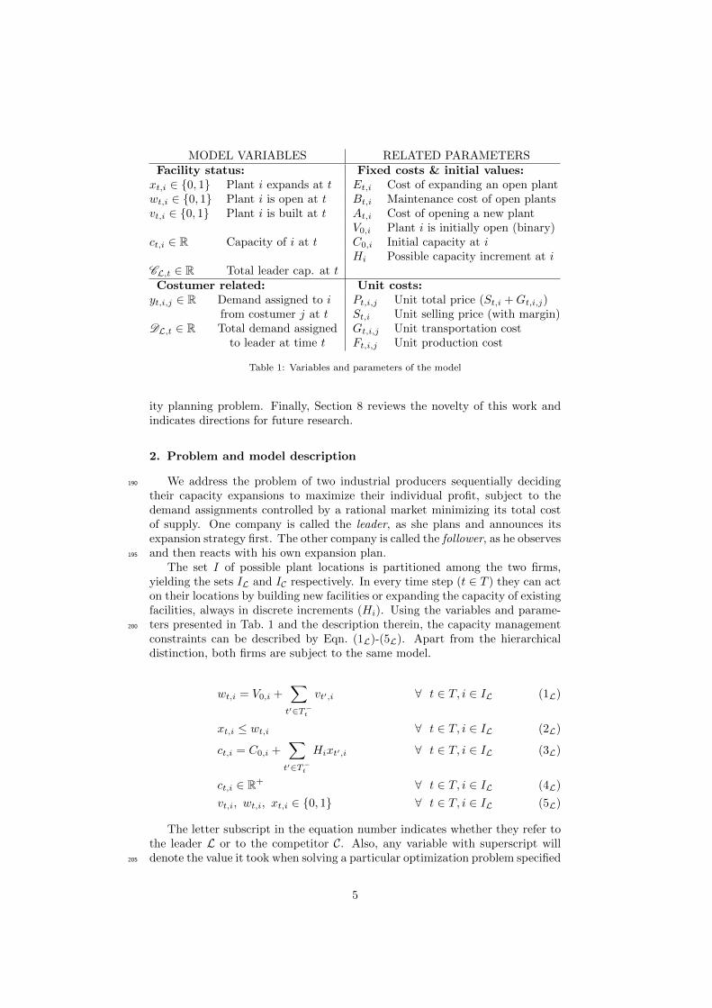
MODEL VARIABLES RELATED PARAMETERSFacility status: Fixed costs & initial values:xt,i ∈ 0, 1 Plant i expands at t Et,i Cost of expanding an open plantwt,i ∈ 0, 1 Plant i is open at t Bt,i Maintenance cost of open plantsvt,i ∈ 0, 1 Plant i is built at t At,i Cost of opening a new plant

V0,i Plant i is initially open (binary)ct,i ∈ R Capacity of i at t C0,i Initial capacity at i

Hi Possible capacity increment at iCL,t ∈ R Total leader cap. at tCostumer related: Unit costs:yt,i,j ∈ R Demand assigned to i

from costumer j at tDL,t ∈ R Total demand assigned

to leader at time t

Pt,i,j Unit total price (St,i +Gt,i,j)St,i Unit selling price (with margin)Gt,i,j Unit transportation costFt,i,j Unit production cost

Table 1: Variables and parameters of the model

ity planning problem. Finally, Section 8 reviews the novelty of this work andindicates directions for future research.

2. Problem and model description

We address the problem of two industrial producers sequentially deciding190

their capacity expansions to maximize their individual profit, subject to thedemand assignments controlled by a rational market minimizing its total costof supply. One company is called the leader, as she plans and announces itsexpansion strategy first. The other company is called the follower, as he observesand then reacts with his own expansion plan.195

The set I of possible plant locations is partitioned among the two firms,yielding the sets IL and IC respectively. In every time step (t ∈ T ) they can acton their locations by building new facilities or expanding the capacity of existingfacilities, always in discrete increments (Hi). Using the variables and parame-ters presented in Tab. 1 and the description therein, the capacity management200

constraints can be described by Eqn. (1L)-(5L). Apart from the hierarchicaldistinction, both firms are subject to the same model.

wt,i = V0,i +∑t′∈T−t

vt′,i ∀ t ∈ T, i ∈ IL (1L)

xt,i ≤ wt,i ∀ t ∈ T, i ∈ IL (2L)

ct,i = C0,i +∑t′∈T−t

Hixt′,i ∀ t ∈ T, i ∈ IL (3L)

ct,i ∈ R+ ∀ t ∈ T, i ∈ IL (4L)

vt,i, wt,i, xt,i ∈ 0, 1 ∀ t ∈ T, i ∈ IL (5L)

The letter subscript in the equation number indicates whether they refer tothe leader L or to the competitor C. Also, any variable with superscript willdenote the value it took when solving a particular optimization problem specified205

5

by the superscript or the context. Other used shorthands include xL to denotethe vector of all leader variables [xt,i, vt,i, wt,i, ct,i]t∈T,i∈IL , XL represents itsdomain, and T−t and T+

t denote all times before or after t respectively. Followingagain the notation from Tab. 1, the objective function of the firms is defined asthe Net Present Value (NPVL or NPVC) given by Eqn. (6L). The first sum is210

the total income of the firm. The second are the fixed costs related to capacityinvestments and maintenance. Finally the third includes the variable costs. Anydesired discount factor is included in the time-varying parameters.

NPVL(xL, y) =∑t∈T

∑i∈IL

∑j∈J

Pt,i,jyt,i,j

−∑t∈T

∑i∈IL

(At,ivt,i +Bt,iwt,i + Et,ixt,i)

−∑t∈T

∑i∈IL

∑j∈J

(Ft,i +Gt,i,j) yt,i,j

(6L)

Note that the only coupling between both companies comes from the demandsyt,i,j each costumer j ∈ J assigns to every facility (i.e. firms do not directly act215

on the opponent’s plants, as in Defender-Attacker problems [34]). Given ourrational market model, these assignments must be a solution of the optimizationproblem solved by the market to minimize its total cost P (y) -Eqn. (7)- ofsatisfying its demand -Eqn. (8)- subject to the available capacities -Eqn. (9).The resulting optimization problem is called the market problem M(c). Its220

solution vector of demand assignments y must lie in the region Ψy(xL, xC),called the market Basic Rational Reaction set as described in Sec. 3.

Ψy(xL, xC) = arg minyt,i,j≥0

P (y) =∑t∈T

∑i∈I

∑j∈J

Pt,i,jyt,i,j (7)

s.t.∑i∈I

yt,i,j = Dt,j ∀ t ∈ T, j ∈ J (8)∑j∈J

yt,i,j ≤ ct,i ∀ t ∈ T, i ∈ I (9)

The only influence of the suppliers’ decisions (xL, xC) is the right hand sideof Eqn. (9): if a highly demanded and saturated plant increases its capacity,it will gain market share - and others will lose it. Therefore, it is the central225

competition point among suppliers and the motivation to expand well locatedplants.

Note that M(c) is a linear transportation model; hence, it is always feasibleas long as

∑j∈J Dt,j ≤

∑i∈I ct,i ∀t ∈ T . Given that we are mainly interested

by the competitive dynamics arising in this hierarchical framework -and less by230

the companies being artificially forced to expand against their profit- we willconsider that the initially installed capacity is always greater than the totaldemand. This can be done without loss of generality. If the two companies donot have that much installed capacity initially (possibly in old, far, unattractiveplants), we can always consider a third party plant, with unlimited capacity but235

very high prices, so the market will keep maximal pressure on the plants of ourtwo competing firms.

6

We also point out that our Stackelberg model is completely deterministicand hence we can also consider without loss of generality all decisions for alltime steps to be taken at the beginning in “open loop” fashion [26].240

Now we have all the pieces to finally state the full model in Eqns. (10)-(14).This is a trilevel program with integer constraints in the two upper level, whichis at the very frontier of the area.

“ maxxL

” NPVL(xL, y) (10)

s.t. (1L)− (5L) (11)

xC ∈ “ arg maxxC

” NPVC(xC , y) (12)

s.t. (1C)− (5C) (13)

y ∈ Ψy(xL, xC) (14)

We have used quotation marks on the “ max ” and “ arg max ” operators toindicate that the model as stated is not yet well defined [40]. Each player only245

controls its own variables, and hence we need to specify how the lower levelplayers will break their ties in case of having multiple globally optima solutions.In other words, if Ψy(xL, xC) or the “ arg max ” do not yield singletons, theperfect information assumption requires that all players know which particularelement of these sets will be selected. This topic has never been thoroughly250

studied in the trilevel case, and it is the subject of our next section.

3. Multilevel programming and degeneracy

For any non-strictly convex minimization problem, there might be severalalternative global optima. In the multilevel case, if for at least one decision ofthe leader, a lower level program exhibits this phenomena, the problem is called255

degenerate. This ambiguity can have a profound impact on the final solution ofthe multilevel problem as two different optimal responses of the follower will givehim the same objective value, but might produce opposed effects on the higherlevels. It is therefore critical to specify how this ambiguities will be resolved,what are the model interpretation of them, and to develop an algorithm that260

converges to the desired solution. The question has only been addressed in thebilevel case, so in this section we start by reviewing some related definitions andthen we extend them to the trilevel case.

3.1. Review on bilevel optimization

When there are no degeneracies in the lower level, we can write a general265

bilevel problem as in Eqns. (15)-(17), where x ∈ X are the variables controlledby the leader and y ∈ Y are the variables controlled by the follower.

maxx∈X

f1(x, y) (15)

s.t. g1(x, y) ≤ 0 (16)

y ∈ Ψ(x) = arg maxy∈Y

f2(x, y) : g2(x, y) ≤ 0 (17)

7

Definition 1. Given the bilevel program presented in Eqns. (15)-(17), let• Ω be the Bilevel Constraint Region:

Ω = (x, y) ∈ X × Y : g1(x, y) ≤ 0, g2(x, y) ≤ 0 (18)

• Ωy(x) be the Follower Constraint Region for a fixed x ∈ X:270

Ωy(x) = y ∈ Y : g2(x, y) ≤ 0 (19)

• Ψ(x) be the Basic Rational Reaction set for a fixed x ∈ X:

Ψ(x) = arg maxy∈Y

f2(x, y) : g2(x, y) ≤ 0 (20)

If Ψ(x) is not a singleton, keeping the formulation as in Eqns. (15)-(17)suggests that the leader also can choose its most favorable y, as long as it isoptimal for the follower. This is called the Optimistic formulation and it is themost common approach in the literature. Formally, we could either write y ∈ Y275

as a variable under the first max or replace Ψ(x) in Eqn. (17) by the BilevelOptimistic Reaction set defined by Eqn. (21). Note that it is irrelevant whetherthis set is now a singleton, given that any point y ∈ ΨL(x) ⊂ Ψ(x) will grantthe same objective value to both players.

ΨL(x) = arg maxy∈Ψ(x)

f1(x, y) (21)

Apart from the mathematical necessity to address the degeneracy issue, it280

is also a modeling concern. The Optimistic approach is adequate when somedegree of collaboration, or “ε-influence”, is allowed between levels -as side-payments from the leader for example. This interpretation and some refor-mulation aspects described in Sec. 4 make it the most commonly widespreadapproach. However, there is an increasing interest on extending the treatment285

of degeneracies, studying other alternative formulations. The Pessimistic ap-proach can be defined as the model in which the lower level selects the responsethat is most detrimental to the leader in case of degeneracy [11]. These al-ternative models are considered harder to solve than the Optimistic approach,although new algorithms are weakening this condition [41].290

The idea outlined in Eqn. (21) of reducing the Basic Rational Reaction setso that it captures the chosen tie breaking strategy, is very powerful and will beextended in the next subsection also to trilevel problems, allowing to formallydefine the possible “Optimistic” formulations.

3.2. Degeneracy in trilevel programming295

In order to comply with the perfect information assumption, the decisioncriteria under degeneracy must be completely specified at all levels. In thisway, decision-makers that are hierarchically higher can calculate the responseof the lower levels. Unfortunately, the definition of bilevel Optimistic solutiondoes not extend trivially to trilevel programs. Next, we propose three mean-300

ingful extensions according to the order in which the objective functions of theupper-levels are favored: Sequentially Optimistic, Hierarchically Optimistic andStrategically Optimistic. The analysis herein is completely general, but for bet-ter use in Sec. 4, we have used the capacity expansion variables and objectivesintroduced in Sec. 2.305

8

Definition 2. The optimal solution to a trilevel program is considered Sequen-tially Optimistic if degeneracy in the third level is resolved in favor of the secondlevel, and degeneracy in the second level is resolved in favor of the first level.

Definition 3. The optimal solution to a trilevel program is considered Hier-archically Optimistic if degeneracy in the third level is resolved in favor of the310

first level, and degeneracy in the second level is also resolved in favor of the firstlevel.

Surprisingly, the Hierarchically Optimistic model for resolving degeneracydoes not guarantee the best possible objective for the first-level decision-maker.Therefore, we present a third optimistic approach to degeneracy.315

Definition 4. The optimal solution to a trilevel program is considered Strategi-cally Optimistic if degeneracy in the second level is resolved in favor of the firstlevel, and degeneracy in the third level is resolved such that the best first-levelsolution is obtained.

For a simple case where these definitions yield different solutions, refer to Ex-320

ample 1 at the end of this section. To characterize mathematically each of thesesolutions, as was outlined in the bilevel case, we will replace the Basic RationalReaction set by the appropriate subset. First let us introduce some notation.The definitions of Trilevel Constraint Region Ω and Third Level Constraint Re-gion Ωy(xL, xC) can be extended directly from the bilevel case in Def. 1. The325

Rational Reaction sets require some more work. Their use will become clear inProp. 1-3, where they enforce the different degeneracy resolution criteria.

Definition 5. In a trilevel program we define the following sets:• The Basic Rational Reaction set of the third level:

Ψy(xL, xC) = arg miny∈Ωy(xL,xC)

P (y) (22)

• The Sequentially Optimistic reaction set of the third level:330

ΨC,y(xL, xC) = arg maxy∈Ψy(xL,xC)

NPVC(xC , y) (23)

• The Hierarchically Optimistic reaction set of the third level:

ΨL,y(xL, xC) = arg maxy∈Ψy(xL,xC)

NPVL(xL, y) (24)

• The Sequentially Optimistic reaction set of the second level:

ΨSeqxC (xL) = arg max

xC∈XC(xL)

NPVC(xL, xC , y) : y ∈ ΨC,y(xL, xC) (25)

• The Hierarchically Optimistic reaction set of the second level:

ΨHiexC (xL) = arg max

xC∈XC(xL)

NPVC(xC , y) : y ∈ ΨL,y(xL, xC) (26)

• The Strategically Optimistic reaction set of the two followers is:

ΨStr(xC,y)(xL) =

(xC , y) ∈ XC(xL)×Ψy(xL, xC) :

∀ xC ∈ XC(xL),∃ y ∈ Ψy(xL, xC) :

NPVC(xC , y) ≥ NPVC(xC , y) (27)

9

Next, we are interested on precisely describing all points (xL, xC , y) that335

satisfy each of the Defs. 2-4. Apart from the theoretical interest, we pointout that most algorithms for multilevel problems essentially solve single levelproblems of the type of Eqns. (15)-(17), somehow enforcing the lower levelvariables to be in their Rational Reaction set. Hence, it is critical to constrainenough the variables of the followers so that their control can be given to the340

leader without waving their rational behavior. In the following, we state whatare these constraints in the case of the three trilevel Optimistic solution typesfrom Defs. 2-4.

Proposition 1. The set of Sequentially Optimistic solutions is:

arg max(xL,xC,y)

NPVL(xL, y) : xL ∈ XL, xC ∈ ΨSeq

xC (xL), y ∈ ΨC,y(xL, xC)

(28)

Proof. The market first breaks its ties in favor of the competitor, as imposed345

by y ∈ ΨSeqC,y (xL, xC). The competitor is aware of it and plans according to

the definition of ΨSeqxC in Eqn. (25). Note that in fact this definition could

simply have y ∈ Ψy(xL, xC) instead of y ∈ ΨC,y(xL, xC), given that the objectivefunction being optimized is NPVC .

Proposition 2. The set of Hierarchically Optimistic solutions is:350

arg max(xL,xC,y)

NPVL(xL, y) : xL ∈ XL, xC ∈ ΨHie

xC (xL), y ∈ ΨL,y(xL, xC)

(29)

Proof. Again, the market is imposed to always break its ties in favor of theleader first, and the competitor plans accordingly.

Proposition 3. The set of Strategically Optimistic solutions is:

arg max(xL,xC,y)

NPVL(xL, xC , y) : xL ∈ XL, (xC , y) ∈ ΨStr

(xC,y)(xL)

(30)

Proof. The idea behind the Strategically Optimistic model is that the resolutionof the degeneracy of the third level is fully controlled by the leader. And the355

competitor knows it. More precisely, for each possible reaction of the competitorxC ∈ XC(xL), the leader could force the market to take a y ∈ Ψy(xL, xC) thatgives him the lowest NPVC(xC , y). Therefore, the competitor is willing to takeany strategy xC as long as the leader commits to steer the market decision yto a point granting him anything higher than the best NPVC(xC , y) he could360

achieve having the market completley against him.

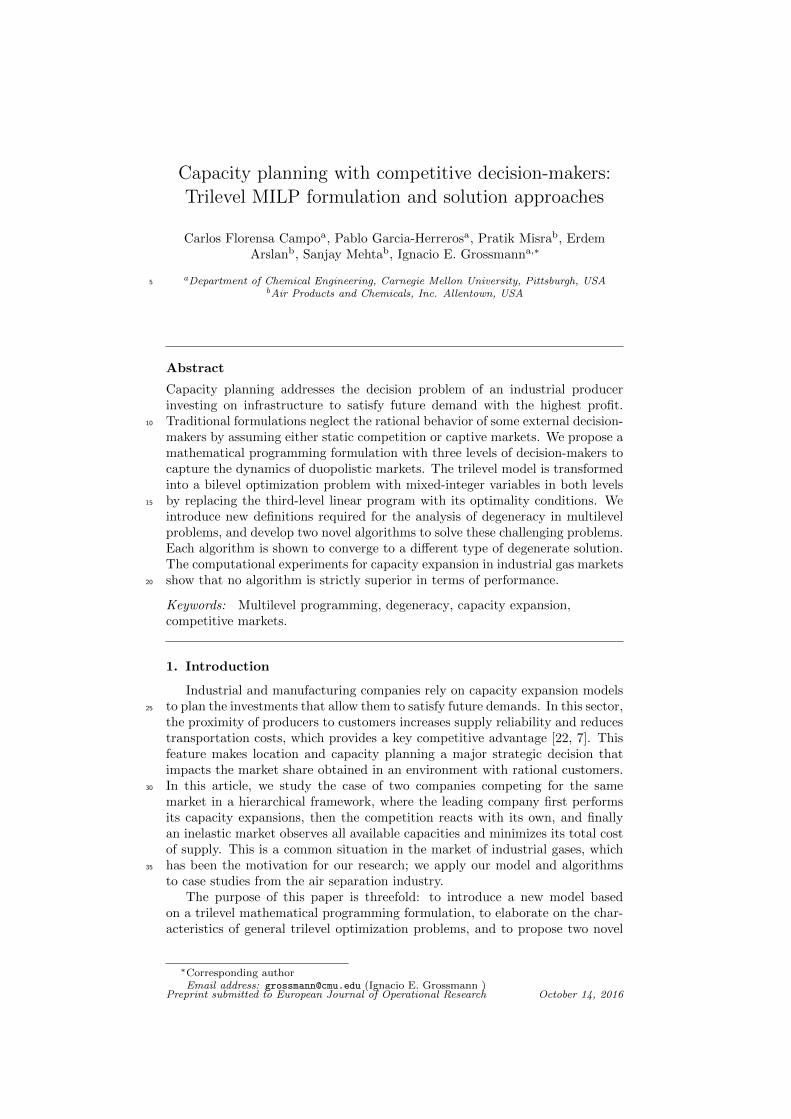
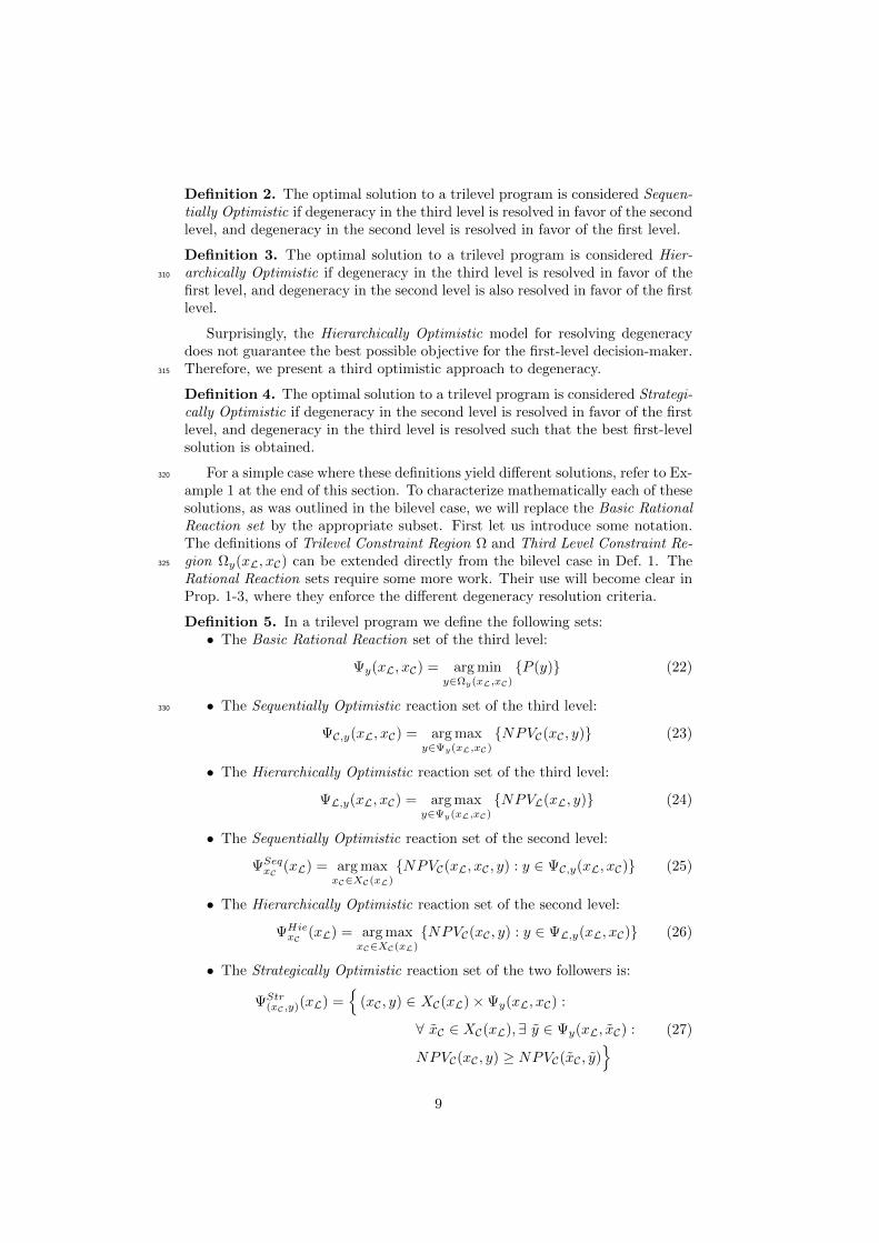
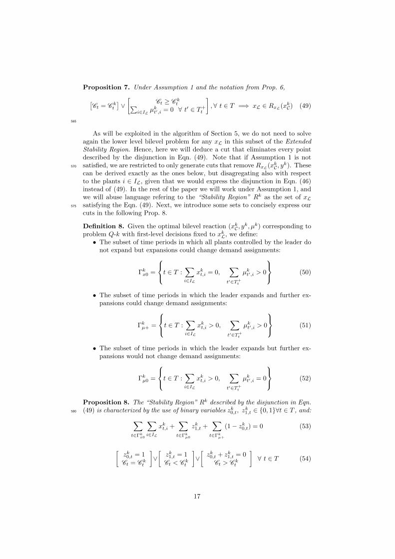
Example 1. We illustrate how all the different Optimistic solution types fromDefs. 2-4 might not coincide. Consider the case depicted in Fig. 1, where fora fixed decision of the leader x1

L, the second level has two feasible startegiesx1C , x

2C , and that in both cases the third level is degenerate and has two possible365

optimal decisions, yA, yB and yC , yD respectively. The objective values ofthe leader NPVL and the follower NPVC for each case are explicited therein.According to them, outcome D is the optimal solution under the SequentiallyOptimistic model because degeneracy in the third level favors the objectiveof the competition (NPVL = 200, NPVC = 400). Under the Hierarchically370

Optimistic model, the optimal solution of the problem is given by outcome C

10

(NPVL = 100, NPVC = 200). This result is counter-intuitive because resolutionof third-level degeneracy locally favors the first level, but it forces the second-level to avoid x1

C and select instead x2C , which is detrimental for the leader. The

Strategically Optimistic solution is outcome A (NPVL = 300, NPVC = 300) and375

in general it is the best the leader can achieve in a trilevel setup. Outcome B willnever happen under any degeneracy resolution model because the competitorwill never accept it (he will rather have any of the outcomes associated withx2C).

𝑥𝑥𝐿𝐿1

𝑥𝑥𝐶𝐶1 𝑥𝑥𝐶𝐶2

𝑁𝑁𝑃𝑃𝑉𝑉𝐿𝐿 = 300𝑁𝑁𝑃𝑃𝑉𝑉𝐶𝐶 = 300

𝑁𝑁𝑃𝑃𝑉𝑉𝐿𝐿 = 400𝑁𝑁𝑃𝑃𝑉𝑉𝐿𝐿 = 100

Third-level degeneracy

Strategically optimistic solution

𝑁𝑁𝑃𝑃𝑉𝑉𝐿𝐿 = 100𝑁𝑁𝑃𝑃𝑉𝑉𝐶𝐶 = 200

𝑁𝑁𝑃𝑃𝑉𝑉𝐿𝐿 = 200𝑁𝑁𝑃𝑃𝑉𝑉𝐶𝐶 = 400

Third-level degeneracy

Sequentially optimistic solution

Hierarchically optimistic solution

A B C D

Figure 1: The Strategically Optimistic model is the most beneficial for the first level. TheSequentially Optimistic is the most beneficial for the second level. The Hierarchical may vary.

Depending on the application, each type of Optimistic solution has a dif-380

ferent interpretation that the modeler needs to be aware of (also to pick theright algorithm). In the particular case of capacity expansion, the Sequentialapproach implies that although we consider undifferentiated products, in case ofa tie for the market the competitor offers a slightly better service. The Hierar-chical is the exact reverse, where inevitably the market would have a preference385

for the leader’s products in case of a tie. Finally, the Strategic implies an addi-tional control of the leader over the market, where she is able to “ε” modify theperception of the market over the products. We have only presented degeneracyresolution models that characterize Optimistic approaches. However, models forPessimistic resolution or mixed resolution (e.g. Optimistic-Pessimistic) can be390

easily extended from our definitions.

4. Three solution paradigms applied to trilevel capacity planning

In this section we recall three concepts from the bilevel literature and outlinehow they will be useful to solve the trilevel capacity planning problem. Firstwe will define the Inducible Region and how for easy problems, like our third395

level LP, it can be found with reformulations. Then, we introduce the HighPoint relaxation and how it can be tightened to yield improving upper bounds.Finally, we study the leader Stability Regions of our problem and define cuts toeliminate them, allowing to accelerate a search over the leader decision space.All the results here will be used to construct the algorithms in Sec. 5-6 and400

prove their convergence to a specific Optimistic trilevel solution.

11

4.1. Inducible Region and reformulations

In bilevel programming, Eqn. (31) defines the Inducible Region (IR) char-acterized by the feasible upper-level decisions and their corresponding rationalresponse in the lower level problem. Therefore, the IR is the feasible region of405

its bilevel program.

IR =

(x, y) : x ∈ X, y ∈ Ψ(x)

(31)

Any degeneration-resolution can be conveyed in Ψ(x). And using the sets in Def.5, this definition can be extended to the trilevel case. An explicit descriptionof the IR would allow solving the problem as a single-level program over it.Unfortunately this region is usually non-convex, non-connected, and in general410

very hard to describe because of the constraint y ∈ Ψ(x). In the simpler case ofhaving a bilevel problem with an LP in the lower level, reformulation techniquescan be used to replace the lower level optimization by its optimality constraints,hence exactly imposing y ∈ Ψ(x). In the following, we detail how to apply thisto reformulate our market problem M(c).415

The most common approach to reformulate a bilevel problem with a convexlower-level is to replace the inner program by its Karush-Kuhn-Tucker (KKT)optimality conditions. However, in linear lower-level problems with inequal-ity constraints, the KKT approach might be ineffective because it requires theaddition of many complementarity constraints. To reformulate our rational mar-ket M(c) described in Eqns. (7)-(9), the duality-based approach described byGarcia-Herreros et al. [15] is better suited because it does not require addingdiscrete variables. The idea is to replace the lower-level LP by constraints guar-anteeing primal feasibility, dual feasibility, and strong duality. Hence, the set ofoptimal solutions to the problem M(c) is described by Eqns. (32)-(36).

∑t∈T

∑i∈I

∑j∈J

Pt,i,jyt,i,j =∑t∈T

∑j∈J

Dt,jλt,j −∑i∈I

ct,iµt,i

(32)

∑j∈J

yt,i,j ≤ ct,i ∀ t ∈ T, i ∈ I (33)

∑i∈I

yt,i,j = Dt,j ∀ t ∈ T, j ∈ J (34)

λt,j − µt,i ≤ Pt,i,j ∀ t ∈ T, i ∈ I, j ∈ J (35)

yt,i,j , µt,i ∈ R+; λt,j ∈ R ∀ t ∈ T, i ∈ I, j ∈ J (36)

where Eqn. (32) enforces strong duality and Eqn. (35) are the dual constraintscorresponding to primal variables yt,i,j . Dual variables associated to Eqn. (9)and Eqn. (8) are denoted by µt,i ∈ R+ and λt,j,k ∈ R, respectively.

It is important to note that Eqn. (32) contains bilinear terms in the productof upper-levels variables ct,i and dual variables µt,i. Bilinear terms are non-420

convex; however, we can apply an exact linearization procedure [16] becausevariables ct,i only take discrete values according to Eqn. (3L) and (3C). Then,a big-M reformulation is applied by introducing new variables ut,t′,i. These areimposed to be the product of dual variables µt,i and expansion variables xt′,i.It can be shown that Eqn. (38) is sufficient when these equations are inside the425

maximization of an NPV (refer to [15] for more details).

12

∑t∈T

∑i∈I

∑j∈J

Pt,i,jyt,i,j =

∑t∈T

∑j∈J

Dt,jλt,j −∑i∈I

C0,iµt,i −∑i∈I

∑t′∈T−t

Hiut,t′,i

(37)

ut,t′,i ≥ µt,i −M(1− xt′,i) ∀ t ∈ T, t′ ∈ T−t , i ∈ I (38)

ut,t′,i ∈ R+ ∀ t ∈ T, t′ ∈ T−t , i ∈ I (39)

Hence, Eqn. (32) can be replaced by Eqns. (37)-(39) and the set of the marketBasic Rational Reaction set Ψy(xL, xC) is completely described by Eqns. (33)-(39). Applied to our present trilevel problem, we can replace Eqn. (14) bythese constraints, obtaining a Bilevel Mixed Integer Linear Program (BMILP)430

with integer variables at both levels. Hence, this problem cannot be furtherreformulated with the same technique and the next subsections introduce newtools.

4.2. High Point relaxation and tightenings

An interesting property of BILPs and BMILPs is that relaxing integrality435

conditions of the lower-level variables does not yield a relaxation of the bilevelproblem (see [30] for a graphical example). Therefore, a special type of relax-ation is required to develop iterative solution methods for these problems. Herewe introduce the High-Point (HP ) relaxation for bilevel programs, which is ob-tained by removing the lower-level objective function but keeping its constraints.440

The resulting single-level problem is a relaxation of the original bilevel problem[30]. In terms of the general bilevel program described by Eqns. (15)-(17), theHigh-Point problem is defined by Eqn. (40).

HP : max(x,y)∈Ω

f1(x, y) (40)

The HP extends to any multilevel problem: removing all lower levels objec-tive functions yields an upper bound. Nevertheless, solving the HP problem445

usually yields a weak upper bound on the original problem because in this re-laxation all variables are controlled by the upper level, waiving any rationalityof the lower levels. And the more rational levels are waived, the worse therelaxation can be expected to be. Hence, we will never use the High-Point re-laxation HPT of the original trilevel problem. Instead, we will do it on the450

BMILP reformulation introduced in the subsection above, calling it HPBMILP

or HP for short. Given that the reformulation already imposes the rationalityof the third level, this is a tighter relaxation. This is formalized in definitionsEqns. (41)-(42) and in Prop. 4.

HPT : max(xL,xC,y)

NPVL(xL, y) : (1L)−(5L), (1C)−(5C), y ∈ Ωy(xL, xC)

(41)

HPBMILP : max(xL,xC,y)

NPVL(xL, y) : (1L)−(5L), (1C)−(5C), (33)−(39)

(42)

13

Proposition 4. The problems HPT and HPBMILP are both relaxations of the455

original trilevel problem, and HPBMILP yields a tighter upper bound than HPT .

Proof. Any feasible solution for the original trilevel problem is obviously fea-sible for these problems, no matter what is the degeneracy resolution chosen.Furthermore, y ∈ Ωy(xL, xC) are the primal constraints of the market, which areexactly Eqns. (33)-(34). Hence, any point feasible for HPBMILP is also feasible460

for HPT yielding the desired result.

Now we present a method to tighten our HP based on the column-and-constraint generation procedure developed by Zeng and An [42]. Their methodtackles general BMILPs by the three steps described below. Notation-wise,remember that any variable with a superscript denotes the value it took when465

solving a particular problem, and hence it is fixed. Just for this paragraph, wealso consider again the general bilevel formulation from Eqns. (15)-(17).

1. Solve the HP problem and collect the solution (xk, yk).

2. Fix the leader variables to xk and solve to optimality the follower’s problemQ-k = Q(xk), obtaining yQ-k.470

3. Add to the HP the equations imposing that the follower has to obtain atleast what it would obtain if its integer variables were fixed to the valuein yQ-k and its continuous variables were optimizing its objective value(imposed with KKT for example). Denote this new problem HP -k or kth

master problem MP -k and iterate.475

This proceedure could be directly applied to solve our BMILP, where theinteger variables of the lower level are exactly the competitor variables xC andthe continuous ones are the market primal and dual variables. Nevertheless,this would be quite inefficient as we would impose the optimality of a set ofvariables that happen to already be involved in equilibrium constraints. Below480

we describe how simply duplicating the constraints with duplicated market (anddual) variables is enough to get as good as a tighening - up to degeneracy.

As above, the idea is to generate constraints that impose the second-levelobjective function NPVC to be at least as large as it would be with any of thesecond-level solutions xkCKk=1 that have been observed. For each of them, thiscan be expressed with Eqn. (43k),

NPVC(xL, xC , y) ≥ NPVC(xL, xkC , yk) (43k)

where yk are duplicate market assignment variables that we want to representhow the market behaves if the competitor chooses xkC and the leader whateverxL. In order to enforce this third-level optimality of demand assignments, a full485

set of duplicate variables (yk, µk, ukλk) and constraints must be appended tothe HP problem for each solution xkC that has been observed. The constraintscorrespond to the duality-based reformulation of the third-level problem; theyare presented in Eqns. (33k)-(39k), where the added superscript k denotes thatall competitor variables have been fixed to xkC .490

Proposition 5. Adding the constraints (43k) and (33k)-(39k) to the HP yieldsa tighter relaxation, for any xkC.

14

Proof. The tightening is obvious as we are simply adding equations. So we needto show that Eqns. (43k) and (33k)-(39k) do not exclude any solution that istrilevel feasible. All first level solutions remain feasible after the constraints are495

appended to the HP problem because we assume that there is always enoughcapacity in the third level to satisfy all demands. Therefore, the duality-basedreformulation of the third level always has a feasible solution for any fixed xLand xkC . Additionally, we can guarantee that no point in the Inducible Region ofthe trilevel problem is excluded from the tightened HP problem, because Eqn.500

(43k) provides lower bounds on NPVC based on solutions that are feasible inthe second and third level problems; solutions in the Inducible Region must beoptimal in the second and third levels, which implies that their correspondingNPVC must be greater or equal than any bound imposed by inequality (43k).Note that Eqns. (43k) and (33k)-(39k) are appended to the HP problem where505

the objective function is NPVL. Therefore, in case of degeneracy it is resolvedby the leader and the rhs of Eqn. (43k) is set to the worst possible outcome forthe competitor. Thus, again it never cuts any trilevel solution, no matter thechosen degeneration resolution. As will be seen in Section 6, this is used to findthe Strategically Optimistic solution.510

4.3. Stability Regions and cuts

To solve a general bilevel program like in Eqns. (15)-(17), the leader hasto know the reaction to each of her actions, or at least to the ones that seemattractive. This burden can be aliviated if the leader can group her actionsx into regions that are certified to produce the same (fixed) reaction yk ∈ Y515

from the follower. This concept has already been used in bilevel optimization[10, 38]. Here, we formalize them by Eqn. (44) and denote them Stability RegionsR(yk) ⊂ X.

R(yk) :=x ∈ X : yk ∈ Ψ(x)

(44)

Once the leader has computed the reaction yk to a certain xk, she doesnot need to re-compute it for any other x ∈ R(yk), and hence these can be520

excluded from any future search. Similarly to the Inducible Region (IR) andthe High Point (HP ) concepts, using the Rational Reaction sets in Defs. 1and 5, we can extend (44) to the trilevel case. Here we first study the regionsRxL(xkC , y

k) ⊂ XL given by Def. 6.

Definition 6. A Stability Region RxL(xkC , yk) is the set of first-level decisions

that produce the same rational reactions (xkC , yk) in the second and third levels.

RxL(xkC , yk) =

xL ∈ XL : (xkC , y

k) ∈ Ψ0xC (xL)×Ψ0

y(xL, xkC)

(45)

where Ψ0xC (xL) and Ψ0

y(xL, xkC) refer to one of the degeneracy resolution models525

described in Section 3.2.

Intuition suggests that in the trilevel capacity planning formulation, expand-ing plants that already have slack capacity do not change the rational responseof the second and third levels. This allows us to exactly describe the stabilityregions with Prop. 6. Refer to Appendix A for the full proof.530

15

Proposition 6. Let Q-k be the bilevel problem obtained after fixing the first-leveldecisions to xkL in the second and third level problems presented in Eqns. (12)-(14). We denote by (xkC , y

k) a corresponding optimal reaction and by µk theoptimal multipliers associated with capacity constraints in Eqn. (9). Then,

xL ∈ RxL(xkC , yk) ⇐⇒

[ct,i = ckt,i

]∨[

ct,i ≥ ckt,iµkt′,i = 0 ∀ t′ ∈ T+

t

],∀ t ∈ T∀i ∈ IL

(46)

As shown at the end of this section, this disjunctive characterization allows togenerate cuts that exclude every point xL in them. Hence, tighter cuts based onRxL(xkC , yk) are not possible: any other expansion decision that is not excludedby these cuts will generate a different reaction, at least from the market.

To deepen this study, we introduce the Extended Stability Regions as the sets535

RxL(xkC), which contain all leader decisions that will not modify the competitor’sreaction.

Definition 7. The Extended Stability Region RxL(xkC) is the set of first leveldecisions that produce the same rational reaction from the second level xC .

RxL(xkC) =xL ∈ XL : ∃y : (xkC , y) ∈ Ψ0

xC (xL)×Ψ0y(xL, x

kC)

(47)

It is clear that RxL(xkC) ⊂ RxL(xkC , yk) ∀yk ∈ Ψy(xL), and hence more pow-

erful cuts could be generated. Nevertheless, two problems should be addressed:

1. A change in the market decision directly affects the leader objective func-540

tion. Hence, it is not clear how the enitre region RxL(xkC) could be cut aswe do with RxL(xkC , y

k).

2. Finding these regions would be equivalent to finding sensitivity conditionsfor the middle level, which happens to have integer variables. It is wellknown that there are no general sensitivity conditions for MILPs; we can-545

not apply duality theory as we could to derive RxL(xkC , yk).

The first issue will be addressed in next Section when the constraint-directedexploration algorithm is presented. The second issue is not solvable in general.Fortunately, introducing Assumption 1 on the leader prices, we can partiallyaddress it and derive stronger cuts in Prop. 7. This is a common modeling550

assumption in the industrial environment, basically stating that each costumersees the leader as a single plant and does not have to worry about what exactplant is serving it.

Assumption 1. All plants controlled by the leader (i ∈ IL) offer unique pricesto each market (j ∈ J).555

Pt,i1,j = Pt,i2,j ∀t ∈ T, (i1, i2) ∈ I2L, j ∈ J (48)

The interest on this assumption is that the market only sees C k, and henceso does the competitor. Therefore, any rearrangement inside the leader, bothin terms of what plants to open or from where to serve the assigned demand,are indifferent -in terms of the objective value- to all the other players. Inparticular, applying the same proof as for Prop. 6, we can show that any internal560

rearrangement of the leader’s capacity will not change the amount of demandassigned to the leader Dt (even though the exact y will vary depending on whereis the capacity), and, hence, the reaction of the competitor will not changeneither.

16

Proposition 7. Under Assumption 1 and the notation from Prop. 6,

[Ct = C k

t

]∨[

Ct ≥ C kt∑

i∈IL µkt′,i = 0 ∀ t′ ∈ T+

t

],∀ t ∈ T =⇒ xL ∈ RxL(xkC) (49)

565

As will be exploited in the algorithm of Section 5, we do not need to solveagain the lower level bilevel problem for any xL in this subset of the ExtendedStability Region. Hence, here we will deduce a cut that eliminates every pointdescribed by the disjunction in Eqn. (49). Note that if Assumption 1 is notsatisfied, we are restricted to only generate cuts that remove RxL(xkC , y

k). These570

can be derived exactly as the ones below, but disagregating also with respectto the plants i ∈ IL, given that we would express the disjunction in Eqn. (46)instead of (49). In the rest of the paper we will work under Assumption 1, andwe will abuse language refering to the “Stability Region” Rk as the set of xLsatisfying the Eqn. (49). Next, we introduce some sets to concisely express our575

cuts in the following Prop. 8.

Definition 8. Given the optimal bilevel reaction (xkC , yk, µk) corresponding to

problem Q-k with first-level decisions fixed to xkL, we define:• The subset of time periods in which all plants controlled by the leader do

not expand but expansions could change demand assignments:

Γkx0 =

t ∈ T :∑i∈IL

xkt,i = 0,∑t′∈T+

t

µkt′,i > 0

(50)

• The subset of time periods in which the leader expands and further ex-pansions could change demand assignments:

Γkµ+ =

t ∈ T :∑i∈IL

xkt,i > 0,∑t′∈T+

t

µkt′,i > 0

(51)

• The subset of time periods in which the leader expands but further ex-pansions would not change demand assignments:

Γkµ0 =

t ∈ T :∑i∈IL

xkt,i > 0,∑t′∈T+

t

µkt′,i = 0

(52)

Proposition 8. The “Stability Region” Rk described by the disjunction in Eqn.(49) is characterized by the use of binary variables zk0,t, z

k1,t ∈ 0, 1∀t ∈ T , and:580 ∑

t∈Γkx0

∑i∈IL

xkt,i +∑t∈Γkµ0

zk1,t +∑t∈Γkµ+

(1− zk0,t) = 0 (53)

[zk0,t = 1Ct = C k

t

]∨[zk1,t = 1Ct < C k

t

]∨[zk0,t + zk1,t = 0

Ct > C kt

]∀ t ∈ T (54)

17

Proof. At any time t ∈ T , the binary variables zk0,t and zk1,t indicate if the leader

offers more, less, or the same capacity than C kt , as expressed by Eqn. (54). The

result follows from combining this with the sets from Def. 8 and the disjunction585

in Eqn. (49) on when the total leader capacity can increase.

A no-good cut to exclude all solutions that belong to this region (xL ∈ Rk)is obtained by forcing the left-hand side of Eqn. (53) to be greater or equal thanone (≥ 1). The next two sections describe how to use this and the other resultsintroduced in this seccion to obtain two solution approaches that converge to590

the different Optimistic solutions.

5. Algorithm 1: Constraint-directed exploration

We use the stability regions of the capacity planning problem and the equa-tions describing them to design a constraint-directed exploration of the leader’sdecision space. Algorithm 1 performs an accelerated search on the inducible595

region by iteratively solving a restricted High-Point problem HP -k, where thecuts from Prop. 8 are added to prevent selecting any leader decision xL belong-ing to any of the previously computed Stability Regions (for which the solutionis known). The details of the algorithm are presented below.

5.1. Reaching the Sequentially Optimistic solution600

After solving the HP -k, the algorithm finds a trilevel feasible solution insidethe stability region Rk where the obtained xHP -k

L lies. This is done by fixing theleader decision to xHP -k

L and solving the single-level reformulation Q-k of thesecond- and third-level problems. From that solution we not only get a lowerbound, but we can now partially describe the Extended Stability Region of this605

observed reaction of the followers Rk by using Prop. 7. Hence, by adding thecuts from Eqn. (53) to the next HP -k+1, the search is directed towards unex-plored first-level decisions. Convergence of the algorithm is guaranteed becausethe problem has a finite number of first-level decisions, and every iteration elim-inates one stability region that contains at least one new point. The operations610

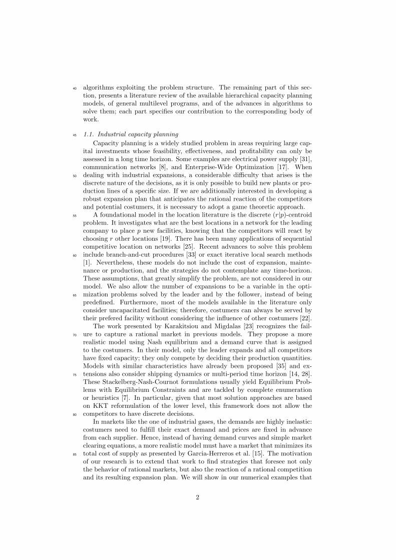
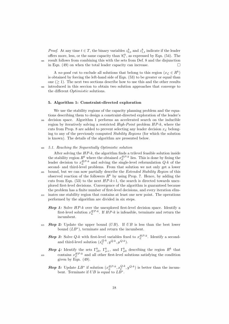
performed by the algorithm are divided in six steps.

Step 1: Solve HP -k over the unexplored first-level decision space. Identify afirst-level solution xHP -k

L . If HP -k is infeasible, terminate and return theincumbent.

Step 2: Update the upper bound (UB). If UB is less than the best lower615

bound (LB∗), terminate and return the incumbent.

Step 3: Solve Q-k with first-level variables fixed to xHP -kL . Identify a second-

and third-level solution (xQ-kC , yQ-k, µQ-k).

Step 4: Identify the sets Γkx0, Γkµ+, and Γkµ0 describing the region Rk that

contains xHP -kL and all other first-level solutions satisfying the condition620

given by Eqn. (49).

Step 5: Update LB∗ if solution (xHP -kL , xQ-k

C , yQ-k) is better than the incum-bent. Terminate if UB is equal to LB∗.

18

Step 6: Generate no-good cuts to exclude Rk from HP -k+1. Go back to Step1.625

Algorithm 1 has two possible stopping criteria:

C1: If UB < LB∗ in Step 2 or Step 5, return incumbent. In this case, nosolution contained in the remaining unexplored region of the first-leveldecision space can be better than the incumbent already found.

C2: If HP -k is infeasible in Step 1, return incumbent. In this case, the first-630

level decision space has been exhaustively analyzed.

It is worth noticing that Step 1 produces an improving UB because thefeasible region of problem HP -k is successively reduced. On the other hand,Step 3 finds a trilevel feasible solution that corresponds to the Sequentially Op-timistic model of degeneracy because problem Q-k resolves degeneracy in favor635

of the second level (y ∈ ΨC,y). A Sequentially Optimistic solution might be verydetrimental for the first level since demands assigned to the leader are degen-erate according to the pricing model presented in Assumption 1. Furthermore,instances with a degenerate third level might not close the gap between UBand LB∗ because problems HP -k and Q-k use different degeneracy resolution640

models. In this case, an exhaustive search could be necessary to meet stop-ping criterion C2 and yield the incumbent, corresponding to the SequentiallyOptimistic solution.

5.2. Reaching the Hierarchically Optimistic solution

Several additional operations are needed to instruct the algorithm to obtain645

the Hierarchically Optimistic solution. The idea is to modify Step 4 to findamong the degenerate solutions the one that favors the leader according to theHierarchically Optimistic model. Two additional optimization problems mustbe defined:• Let HP -kR(xQ-k

C ) be the High-Point problem HP -k constrained to the650

region xL ∈ Rk, and with second-level variables fixed to xQ-kC

• Let HP -kR(NPVC) be the High-Point problem HP -k constrained to xL ∈Rk, and with second-level objective value fixed to NPVC(xHP -k

L ,xQ-kC ,yQ-k).

Solving HP -kR(xQ-kC ) has two purposes: first, to find the best first-level

solution in xL ∈ Rk knowing that the second-level response will be xC . This655

also re-organizes the third level assignments to the leader as to fit the best supplyscheme for her -without affecting the benefit of the market. Second, to detectif the market is degenerate in the sense of having different optimal assignmentsthat yield different NPVC . This is the case if the new solution yHP -kR hasa different aggregated demand to every competitor’s plant. If it is the case,660

we cannot conclude anything about the solution (xHP -kRL , xQ-k

C , yHP -kR) beingtrilevel hierarchically feasible because, if the competitor knew that the marketwould directly favor the leader, he might choose another expansion plan xC .Hence, a penalty must be applied to the market in favor of the leader and goback to Step 3. Notice that by how the prices are constructed, it is enough to665

check that the total aggregated demand to the leader DL,t is the same for allt (if there are changes from one plant to another it can be proven that thereis another optimal solution for the market that yields the same assignments tothe competitor as in Q-k).

19

If the market is not found to be degenerate (or it was solved by a penalty),670

we still have to check whether the second level is degenerate in the sense ofhaving another possible expansion xC that yields the same value for him but abetter one for the leader. This is checked by solving HP -kR(NPVC), and if theobjective value of the leader changes, we need to add a penalty to the competitorand go back to step 3. A detailed description of the steps required to reach the675

Hierarchically Optimistic solution are presented below.

Step 4a: Identify the sets Γkx0, Γkµ+, and Γkµ0 describing the region Rk that

contains xHP -kL and all other first-level solutions satisfying the condition

given by Eqn. (49).

Step 4b: Solve HP -kR(xQ-kC ) and identify the third-level response (yHP -kR). If680

the third-level solution is “aggregately different” from the one obtained in

Step 3 (∃t ∈ T : DHP -kR(xQ-k

C )L,t 6= DQ-k

L,t ), add a penalty to the third-levelobjective to resolve degeneracy in favor of the first level. Go to Step 3.

Step 4c: Solve HP -kR(NPVC). If the first-level objective is different from theone in Step 3 (NPVL(xHP -k

L ,xQ-kC ,yQ-k) 6= NPVL(xHP -kR

L ,xQ-kC ,yHP -kR)), add685

a penalty to the second-level objective to resolve degeneracy in favor ofthe first level. Go to Step 3.

The steps of the algorithm are presented schematically in Fig. 2; diamondscontrol the flow of the algorithm, light gray boxes are simple operations anddark gray boxes involve optimization problems.690

6. Algorithm 2: Column-and-constraint generation algorithm

As opposed to Algorithm 1, Algorithm 2 finds optimal trilevel solutionsby exploring the decision space of the second-level problem. Algorithm 2 isinspired in the column-and-constraint generation algorithm developed by Zengand An [42] for linear bilevel problems with mixed-integer variables in both695

levels. However, our algorithm operates over the bilevel reformulation of thetrilevel capacity planning problem, which already enforces optimality of thevariables controlled by the markets; therefore, no additional reformulation isneeded for the continuous variables. The details of the algorithm are presentedbelow.700

6.1. Reaching the Strategically Optimistic solution

Algorithm 2 uses the tightening presented in Section 4.2 to sequentiallystrengthen the High-Point relaxation of the trilevel capacity planning problem.The algorithm iterates between a master problem MP -k that provides upperbounds UP k and the single-level reformulation of the second- and third-level705

problems with extra cuts Q-k. Problem MP -k is the High-Point relaxationof the bilevel reformulation with the cuts modeled by Eqns. (43k) and (33k)-(39k). The search in Q-k is directed towards unexplored second-level decisionsby adding no-good cuts to the problem Q-k, such that second-level decisionsthat were already observed are not considered in future iterations. These cuts710

are presented in Eqn. (55).

20

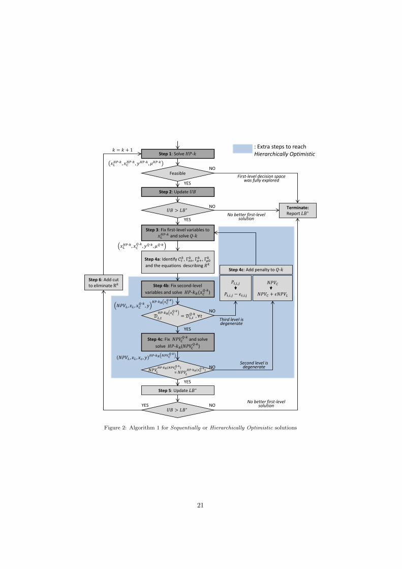
Step 1: Solve𝐻𝐻𝑃𝑃-𝑘𝑘

Step 4a: Identify 𝒞𝒞𝑡𝑡𝑘𝑘, Γ𝑥𝑥𝑥𝑥𝑘𝑘 , Γ𝜇𝜇+𝑘𝑘 , Γ𝜇𝜇0𝑘𝑘

and the equations describing 𝑅𝑅𝑘𝑘

Step 4b: Fix second-levelvariables and solve 𝐻𝐻𝑃𝑃-𝑘𝑘𝑅𝑅(𝑥𝑥𝐶𝐶

𝑄𝑄-𝑘𝑘)

Step 3: Fix first-level variables to 𝑥𝑥𝐿𝐿𝐻𝐻𝐻𝐻-𝑘𝑘 and solve 𝑄𝑄-𝑘𝑘

𝑥𝑥𝐿𝐿𝐻𝐻𝐻𝐻-𝑘𝑘 , 𝑥𝑥𝐶𝐶𝑄𝑄-𝑘𝑘 ,𝑦𝑦𝑄𝑄-𝑘𝑘 ,𝜇𝜇𝑄𝑄-𝑘𝑘

Step 5: Update 𝐿𝐿𝐵𝐵∗

𝑘𝑘 = 𝑘𝑘 + 1

Step 2: Update 𝑈𝑈𝐵𝐵

First-level decision spacewas fully explored

No better first-levelsolution

𝑈𝑈𝐵𝐵 > 𝐿𝐿𝐵𝐵∗

Feasible

𝑥𝑥𝐿𝐿𝐻𝐻𝐻𝐻-𝑘𝑘 , 𝑥𝑥𝐶𝐶𝐻𝐻𝐻𝐻-𝑘𝑘 ,𝑦𝑦𝐻𝐻𝐻𝐻-𝑘𝑘 , 𝜇𝜇𝐻𝐻𝐻𝐻-𝑘𝑘

NO

YES

Third level isdegenerate

𝑈𝑈𝐵𝐵 > 𝐿𝐿𝐵𝐵∗YES

No better first-levelsolution

YES

YES

NO

NO

NO

Step 4c: Fix 𝑁𝑁𝑃𝑃𝑁𝑁𝐶𝐶𝑄𝑄-𝑘𝑘 and solve

solve 𝐻𝐻𝑃𝑃-𝑘𝑘𝑅𝑅(𝑁𝑁𝑃𝑃𝑁𝑁𝐶𝐶𝑄𝑄-𝑘𝑘)

Second level isdegenerateNO

YES

Step 4c: Add penalty to 𝑄𝑄-𝑘𝑘

𝑁𝑁𝑃𝑃𝑁𝑁𝐶𝐶

𝑁𝑁𝑃𝑃𝑁𝑁𝐶𝐶 + 𝜖𝜖𝑁𝑁𝑃𝑃𝑁𝑁𝐿𝐿

𝑃𝑃𝑡𝑡,𝑖𝑖,𝑗𝑗

𝑃𝑃𝑡𝑡,𝑖𝑖,𝑗𝑗 − 𝜖𝜖𝑡𝑡,𝑖𝑖,j

= 𝑁𝑁𝑃𝑃𝑁𝑁𝐿𝐿𝐻𝐻𝐻𝐻-𝑘𝑘𝑅𝑅(𝑥𝑥𝐶𝐶

𝑄𝑄-𝑘𝑘)

Terminate:Report 𝐿𝐿𝐵𝐵∗

Step 6: Add cutto eliminate R𝑘𝑘

𝑁𝑁𝑃𝑃𝑁𝑁𝐿𝐿,𝑥𝑥𝐿𝐿 ,𝑥𝑥𝐶𝐶𝑄𝑄-𝑘𝑘 ,𝑦𝑦

𝐻𝐻𝐻𝐻-𝑘𝑘𝑅𝑅 𝑥𝑥𝐶𝐶𝑄𝑄-𝑘𝑘

𝑁𝑁𝑃𝑃𝑁𝑁𝐿𝐿 ,𝑥𝑥𝐿𝐿 ,𝑥𝑥𝑐𝑐 ,𝑦𝑦 𝐻𝐻𝐻𝐻-𝑘𝑘𝑅𝑅 𝑁𝑁𝐻𝐻𝑁𝑁𝐶𝐶𝑄𝑄-𝑘𝑘

𝒟𝒟𝐿𝐿,𝑡𝑡𝐻𝐻𝐻𝐻-𝑘𝑘𝑅𝑅 𝑥𝑥𝐶𝐶

𝑄𝑄-𝑘𝑘

= 𝒟𝒟𝐿𝐿,𝑡𝑡𝑄𝑄-𝑘𝑘 ,∀𝑡𝑡

𝑁𝑁𝑃𝑃𝑁𝑁𝐿𝐿𝐻𝐻𝐻𝐻-𝑘𝑘𝑅𝑅(𝑁𝑁𝐻𝐻𝑁𝑁𝐶𝐶

𝑄𝑄-𝑘𝑘)

: Extra steps to reach Hierarchically Optimistic

Figure 2: Algorithm 1 for Sequentially or Hierarchically Optimistic solutions

21

∑i∈IC

∑t: xQ-k′

t,i =1

(1− xt,i) +∑

t: xQ-k′t,i =0

xt,i

≥ 1 ∀ k′ ∈ K (55)

where K = 1, 2, . . . , k, and xQ-k′

t,i denotes the values of a second-level optimal

solution for problem Q-k′.The algorithm is identified as a column-and-constraint generation approach

because at every iteration, a new second-level candidate solution (xQ-kC ) is ap-715

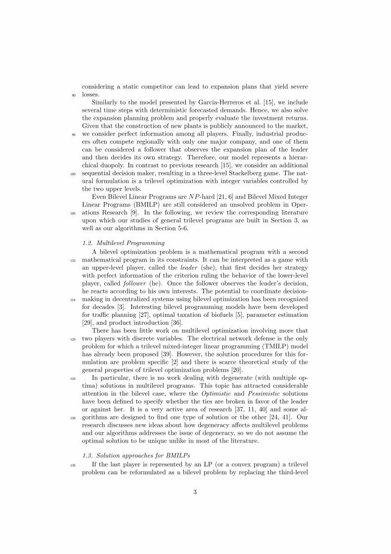
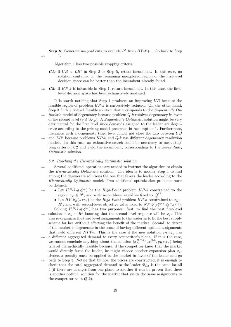
pended to MP -k, together with the constraints and variables modeling thethird-level optimal response. Convergence of Algorithm 2 is guaranteed becausethe problem has a discrete number of second-level decisions, which implies thata finite number of different columns and constraints can be added to MP -k.The operations performed by Algorithm 2 are divided into five steps.720

Step 1: Solve MP -k. Identify the first-level solution (xMP -kL ) and the second-

level objective value NPVC(xMP -kL ,xMP -k

C ,yMP -k).

Step 2: Update the upper bound (UB). If UB is less than or equal to the bestlower bound (LB∗), terminate and return the solution yielding LB∗.

Step 3: Fix first-level variables to xMP -kL and solve Q-k, which is Q-kR includ-725

ing the no-good cuts from Eqn. (55). If infeasible, terminate and returnthe solution yielding UB. Otherwise, identify the second-level solution

(xQ-kC ). If NPVC(xMP -k

L ,xQ-kC ,yQ-k) < NPVC(xMP -k

L ,xMP -kC ,yMP -k), terminate

and return the solution yielding UB.

Step 4: Update the best LB∗. If UB is less or equal to the best lower bound730

(LB∗), terminate and return the solution yielding LB∗.

Step 5: Generate the columns and constraints tightening MP k+1 and the cuts

to exclude xQ-kC from Q-k+1. Go back to Step 1.

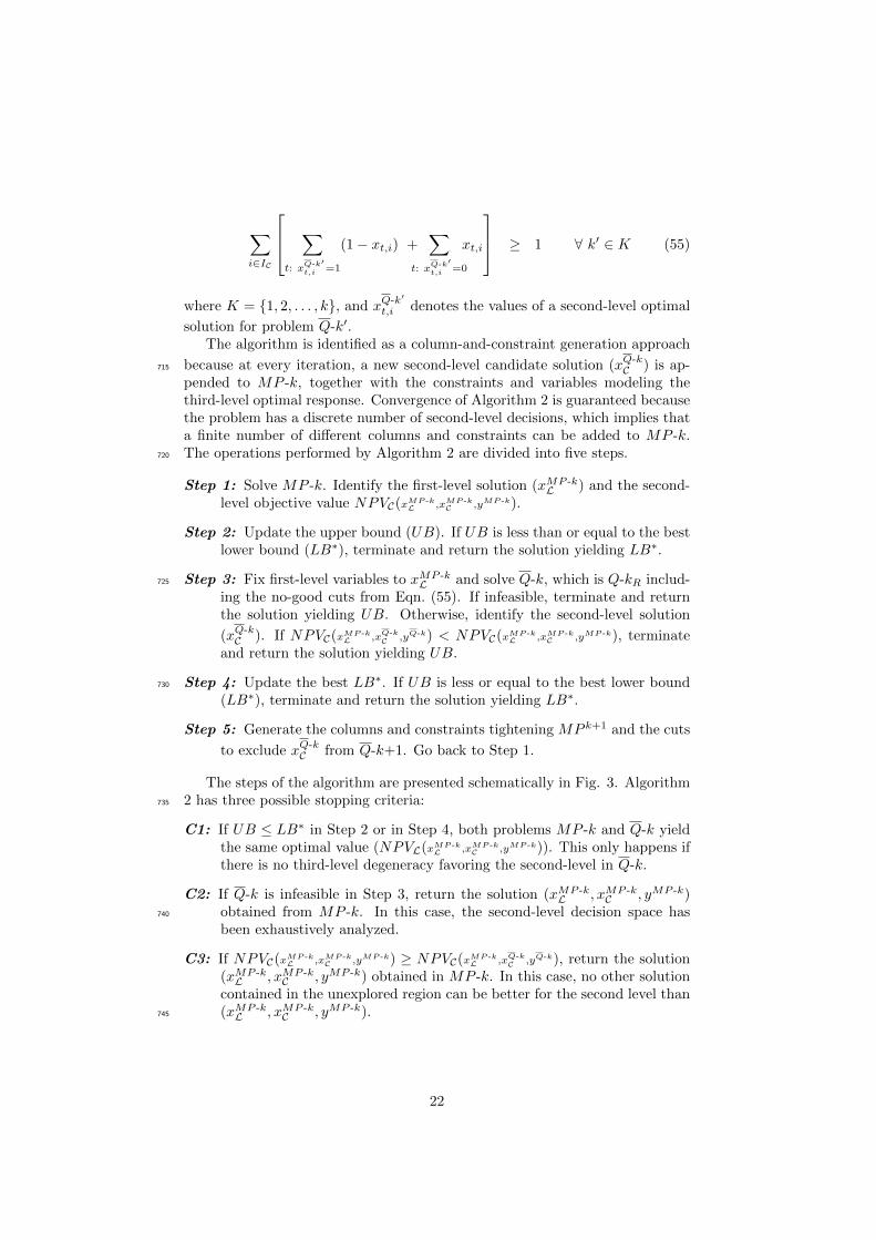
The steps of the algorithm are presented schematically in Fig. 3. Algorithm2 has three possible stopping criteria:735

C1: If UB ≤ LB∗ in Step 2 or in Step 4, both problems MP -k and Q-k yieldthe same optimal value (NPVL(xMP -k

L ,xMP -kC ,yMP -k)). This only happens if

there is no third-level degeneracy favoring the second-level in Q-k.

C2: If Q-k is infeasible in Step 3, return the solution (xMP -kL , xMP -k

C , yMP -k)obtained from MP -k. In this case, the second-level decision space has740

been exhaustively analyzed.

C3: If NPVC(xMP -kL ,xMP -k

C ,yMP -k) ≥ NPVC(xMP -kL ,xQ-k

C ,yQ-k), return the solution(xMP -kL , xMP -k

C , yMP -k) obtained in MP -k. In this case, no other solutioncontained in the unexplored region can be better for the second level than(xMP -kL , xMP -k

C , yMP -k).745

22

No better second-levelsolution

No better first-levelsolution

No better first-levelsolution

Step 1: Solve𝑀𝑀𝑃𝑃-𝑘𝑘

Step 5: Add equationsassociated to 𝑥𝑥𝐶𝐶

𝑄𝑄-𝑘𝑘

𝑥𝑥𝐿𝐿𝑀𝑀𝐻𝐻-𝑘𝑘 , 𝑥𝑥𝐶𝐶𝑄𝑄-𝑘𝑘 ,𝑦𝑦 𝑄𝑄-𝑘𝑘

Step 4: Update 𝐿𝐿𝐵𝐵∗

𝑘𝑘 = 𝑘𝑘 + 1

Step 2: Update 𝑈𝑈𝐵𝐵 Terminate: Report 𝐿𝐿𝐵𝐵∗

𝑥𝑥𝐿𝐿𝑀𝑀𝐻𝐻-𝑘𝑘 , 𝑥𝑥𝐶𝐶𝑀𝑀𝐻𝐻-𝑘𝑘 ,𝑦𝑦𝑀𝑀𝐻𝐻-𝑘𝑘

YES

YES

YES

𝑈𝑈𝐵𝐵 > 𝐿𝐿𝐵𝐵∗

𝑘𝑘 = 𝑘𝑘 + 1

𝑁𝑁𝑃𝑃𝑁𝑁𝐶𝐶𝑀𝑀𝐻𝐻-𝑘𝑘 < 𝑁𝑁𝑃𝑃𝑁𝑁𝐶𝐶𝑄𝑄-𝑘𝑘

NO

𝑈𝑈𝐵𝐵 > 𝐿𝐿𝐵𝐵∗

Second-level decisionspace was fully explored

Feasible?

YES

NO

NO

NO

Terminate: Report 𝑈𝑈𝐵𝐵

Step 3: Fix first-level variables to 𝑥𝑥𝐿𝐿𝑀𝑀𝐻𝐻-𝑘𝑘 and solve 𝑄𝑄-𝑘𝑘No-good cut

Constraint generation

Figure 3: Algorithm 2 for Strategically Optimistic solution

It is worth noticing that Step 1 produces an improving UB because the fea-sible region of problem HP -k is successively reduced according to Prop. 5. Also,the solutions obtained from HP -k correspond to Strategically Optimistic modelof degeneracy since the control of all variables is granted to the first level andonly a constraint on the second-level objective value is imposed. Neverhteless,750

Step 3 resolves third-level degeneracy in favor of the second level. Consequently,the gap between UB and LB∗ might not close; in this case, either criterion C2or C3 will be met.

Remark. Algorithm 1 and Algorithm 2 are guaranteed to find the same trileveloptimal solution in instances with no degeneracy at any level. If degeneracy is755

present, no result can be established about the relative performance of the al-gorithms because they seek for different solutions, and these two problems canbe arbitrarily difficult to solve with respect to the other. For non-degenerateinstances we can establish that Algorithm 1 requires at least the same numberiterations as Algorithm 2. This is the case because Algorithm 2 explores at most760

one point in each Extended Stability Region, which is not true for Algorithm 1(remember that Prop. 7 only provided one direction of the implication). How-ever, it does not imply that Algorithm 2 outperforms Algorithm 1 in executiontime because Algorithm 2 adds many variables and constraints to MP -k atevery iteration, which increases the complexity of the iterations.765

23

7. Capacity planning instances

We test Algorithms 1 and 2 using two instances of the capacity planningproblem with competitive decision-makers. The algorithms are implemented tofind the Hierarchically and Strategically Optimistic solutions, respectively. Thefirst instance is an illustrative example that we use to provide insight about the770

performance of the algorithms; the second instance is an industrial example ofpractical interest for the air separation industry.

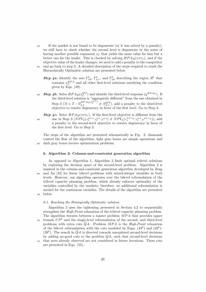
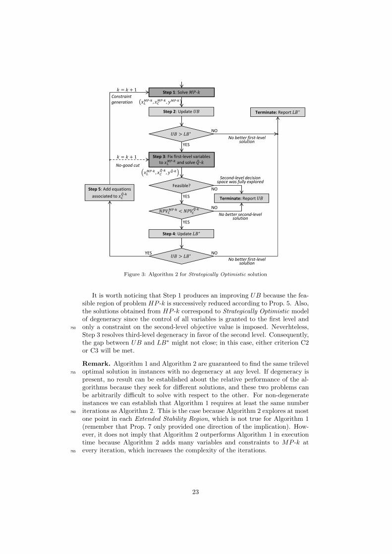
Instance 1. Illustrative instance of trilevel capacity planningThis example considers one existing plant (L1) and one potential plant (L2)

controlled by the leader, as well as one existing plant (C1) and one potential775

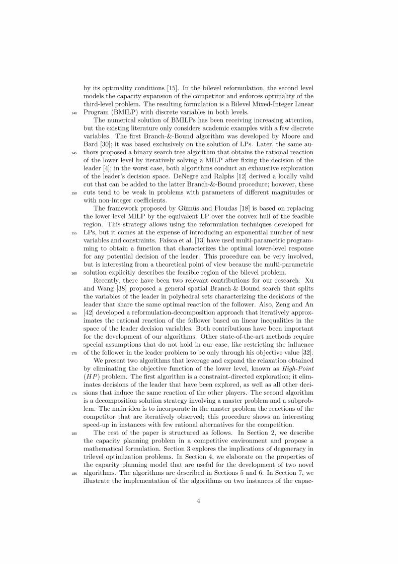
plant (C2) controlled by the competition. The market comprises four customers(Mj) with demands for a single commodity. The planning problem has a horizonof 20 time periods in which the plants are allowed to expand in periods 1, 5,9, 13, and 17. A scheme representing the location of plants and markets ispresented in Fig. 4; the parameters of the instance are given in Tables 2, 3, and780

4.

𝓛1

𝑃 =9𝓛2

𝓒1

𝓒2

𝑴𝟑𝑴𝟏

𝑴𝟒

𝑴𝟐

𝑃 =8

𝑃 =8𝑃 =8

Figure 4: Network of plants and markets inInstance 1

Time (t)Customer (j)

Dt,1 Dt,2 Dt,3 Dt,4

1-4 3.75 0 3 105-8 3.75 0 3 109-12 3.75 8 3 1013-16 3.75 10 3 1017-20 3.75 10 3 10

Table 2: Market demands [M ton/period] inInstance 1

Costumer(j)

Plant (i)Pt,L1,j Pt,L2,j Pt,C1,j Pt,C2,j

M1 8 8 17 17M2 8 8 9 17M3 17 17 8 17M4 9 9 10 8

Table 3: Selling prices [$/ton] in Instance 1

ParameterPlant (i)

L1 L2 C1 C2At,i [M$] - 0 - 0Bt,i [M$/time] 15 15 15 15Et,i [M$/exp] 110 110 110 110Ft,i [$/ton] 3 3 2 4Gt,i,1 [$/ton] 1 10 10 10Gt,i,2 [$/ton] 10 1 2 10Gt,i,3 [$/ton] 10 10 1 10Gt,i,4 [$/ton] 10 2 3 1C0,i [ton] 3.75 0 30 0Ht,i [ton/exp] 30 30 30 30

Table 4: Cost parameters and initial capaci-ties in Instance 1

The optimal expansion strategy for the leader induces expanding plant L2 attime 9 to capture the demand from M2. The rational reaction of the competitionis to expand plant C2 at time 9 to maintain M4 by offering a lower price than theleader. The elements of the objective functions at the trilevel optimal solution785

are presented in Table 5.Instance 1 has been designed such that Algorithms 1 and 2 find exactly the

same solution at every iteration. This is possible because the Hierarchicallyand Strategically Optimistic solutions coincide (no degeneracy) and because thedifferent restrictions on the HP in the two algorithms happen to have the same790

solution at every step of this instance. The convergence of the upper and lowerbounds for both algorithms can be observed in Fig. 5.

24

Items of objective function Leader Competition

Income from sales [M$]: 1,496 2,240Expansion cost [M$]: 110 110Maintenance cost [M$]: 480 480Production cost [M$]: 561 760Transportation cost [M$]: 187 420

Total NPV [M$]: 158 470

Table 5: Optimal objective values in Instance 1

1 2 3 4 5

200

400

600

800

Iteration (k)

Ob

ject

ive

valu

e[M

$]

Upper boundLower bound

Figure 5: Convergence of Algorithms 1 and 2 in Instance 1

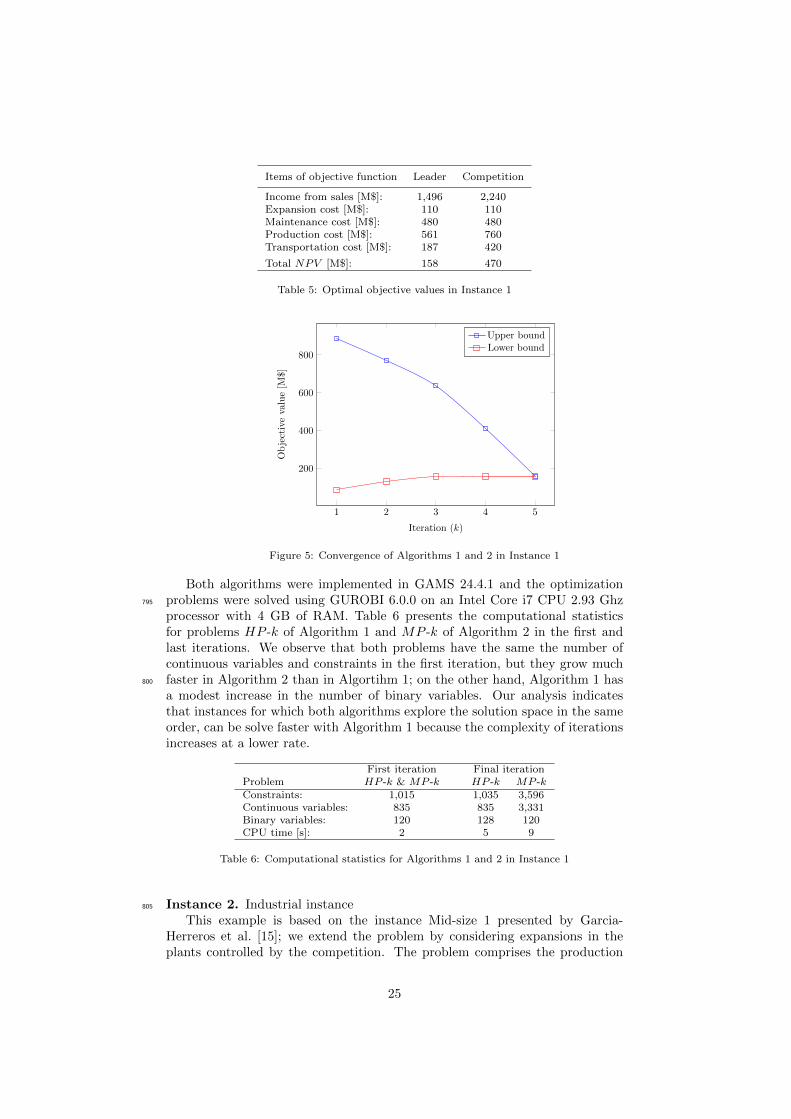
Both algorithms were implemented in GAMS 24.4.1 and the optimizationproblems were solved using GUROBI 6.0.0 on an Intel Core i7 CPU 2.93 Ghz795

processor with 4 GB of RAM. Table 6 presents the computational statisticsfor problems HP -k of Algorithm 1 and MP -k of Algorithm 2 in the first andlast iterations. We observe that both problems have the same the number ofcontinuous variables and constraints in the first iteration, but they grow muchfaster in Algorithm 2 than in Algortihm 1; on the other hand, Algorithm 1 has800

a modest increase in the number of binary variables. Our analysis indicatesthat instances for which both algorithms explore the solution space in the sameorder, can be solve faster with Algorithm 1 because the complexity of iterationsincreases at a lower rate.

First iteration Final iterationProblem HP -k & MP -k HP -k MP -kConstraints: 1,015 1,035 3,596Continuous variables: 835 835 3,331Binary variables: 120 128 120CPU time [s]: 2 5 9

Table 6: Computational statistics for Algorithms 1 and 2 in Instance 1

Instance 2. Industrial instance805

This example is based on the instance Mid-size 1 presented by Garcia-Herreros et al. [15]; we extend the problem by considering expansions in theplants controlled by the competition. The problem comprises the production

25

and distribution of one product to 15 customers. Initially, the leader has threeplants with initial capacities equal to 27,000 ton/period, 13,500 ton/period, and810

31,500 ton/period. Additionally, the leader considers the possibility of open-ing a new plant at a candidate location. As for the competition, he controlsthree plants with an initial capacity of 22,500 ton/period, 45,000 ton/periodand 49,500 ton/period; the competition also has a candidate location for a newplant. The investment decisions are evaluated over a time horizon of 5 years815

divided in 20 time periods; all producers are allowed to expand only every fourthtime-period.

Selling prices and market demands follow an increasing trend during thetime horizon. Investment and maintenance costs grow in time to adjust forinflation. The costs of production also have an increasing trend but exhibit820

a seasonal variation that relate to electricity prices. The exact data for thisindustrial instance can be found in the Supplementary material.

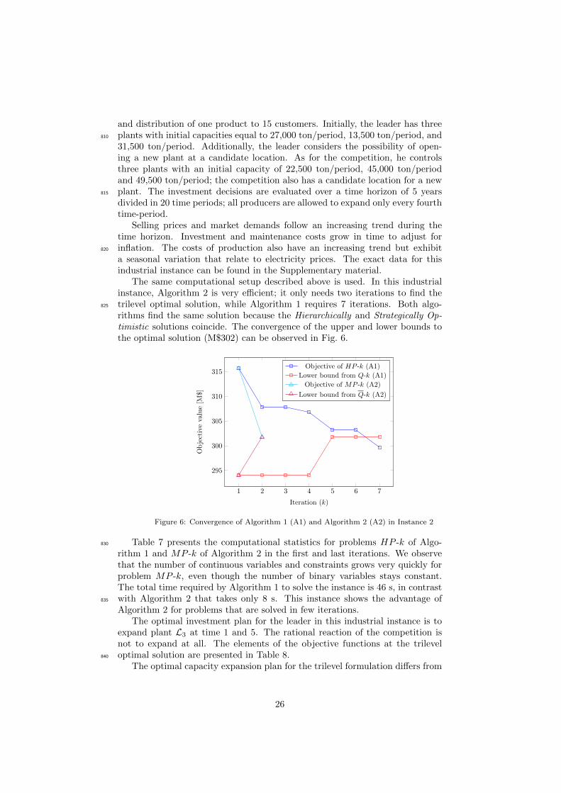
The same computational setup described above is used. In this industrialinstance, Algorithm 2 is very efficient; it only needs two iterations to find thetrilevel optimal solution, while Algorithm 1 requires 7 iterations. Both algo-825

rithms find the same solution because the Hierarchically and Strategically Op-timistic solutions coincide. The convergence of the upper and lower bounds tothe optimal solution (M$302) can be observed in Fig. 6.

1 2 3 4 5 6 7

295

300

305

310

315

Iteration (k)

Ob

ject

ive

valu

e[M

$]

Objective of HP -k (A1)

Lower bound from Q-k (A1)

Objective of MP -k (A2)

Lower bound from Q-k (A2)

Figure 6: Convergence of Algorithm 1 (A1) and Algorithm 2 (A2) in Instance 2

Table 7 presents the computational statistics for problems HP -k of Algo-830

rithm 1 and MP -k of Algorithm 2 in the first and last iterations. We observethat the number of continuous variables and constraints grows very quickly forproblem MP -k, even though the number of binary variables stays constant.The total time required by Algorithm 1 to solve the instance is 46 s, in contrastwith Algorithm 2 that takes only 8 s. This instance shows the advantage of835

Algorithm 2 for problems that are solved in few iterations.The optimal investment plan for the leader in this industrial instance is to

expand plant L3 at time 1 and 5. The rational reaction of the competition isnot to expand at all. The elements of the objective functions at the trileveloptimal solution are presented in Table 8.840

The optimal capacity expansion plan for the trilevel formulation differs from

26

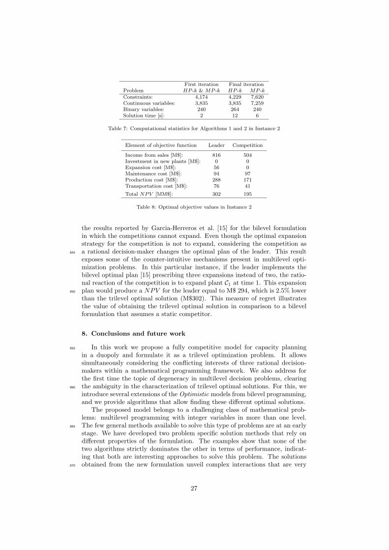
First iteration Final iterationProblem HP -k & MP -k HP -k MP -kConstraints: 4,174 4,229 7,620Continuous variables: 3,835 3,835 7,259Binary variables: 240 264 240Solution time [s]: 2 12 6

Table 7: Computational statistics for Algorithms 1 and 2 in Instance 2

Element of objective function Leader Competition

Income from sales [M$]: 816 504Investment in new plants [M$]: 0 0Expansion cost [M$]: 56 0Maintenance cost [M$]: 94 97Production cost [M$]: 288 171Transportation cost [M$]: 76 41

Total NPV [MM$]: 302 195

Table 8: Optimal objective values in Instance 2

the results reported by Garcia-Herreros et al. [15] for the bilevel formulationin which the competitions cannot expand. Even though the optimal expansionstrategy for the competition is not to expand, considering the competition asa rational decision-maker changes the optimal plan of the leader. This result845

exposes some of the counter-intuitive mechanisms present in multilevel opti-mization problems. In this particular instance, if the leader implements thebilevel optimal plan [15] prescribing three expansions instead of two, the ratio-nal reaction of the competition is to expand plant C1 at time 1. This expansionplan would produce a NPV for the leader equal to M$ 294, which is 2.5% lower850

than the trilevel optimal solution (M$302). This measure of regret illustratesthe value of obtaining the trilevel optimal solution in comparison to a bilevelformulation that assumes a static competitor.

8. Conclusions and future work

In this work we propose a fully competitive model for capacity planning855

in a duopoly and formulate it as a trilevel optimization problem. It allowssimultaneously considering the conflicting interests of three rational decision-makers within a mathematical programming framework. We also address forthe first time the topic of degeneracy in multilevel decision problems, clearingthe ambiguity in the characterization of trilevel optimal solutions. For this, we860

introduce several extensions of the Optimistic models from bilevel programming,and we provide algorithms that allow finding these different optimal solutions.

The proposed model belongs to a challenging class of mathematical prob-lems: multilevel programming with integer variables in more than one level.The few general methods available to solve this type of problems are at an early865

stage. We have developed two problem specific solution methods that rely ondifferent properties of the formulation. The examples show that none of thetwo algorithms strictly dominates the other in terms of performance, indicat-ing that both are interesting approaches to solve this problem. The solutionsobtained from the new formulation unveil complex interactions that are very870

27

difficult to predict. A significant improvement over previously proposed modelsis quantified in economic terms for the industrial instance.

The type of problems that we address are of interest in applications wherediscrete decisions are taken by different players in a hierarchy. As the rangeof applications is expected to increase, we consider the generalization of the875

algorithms as an important direction for future research. Additionally, efficiencyand numerical stability of the algorithms can still improve. For the industrialapplication of the capacity expansion model, we believe that it is importantto extend the model to include stochastic parameters like demand forecasts orcosts. In the case of using the model for different market environments, it might880

be interesting to modify the competition assumption to be Nash-Cournot, whilestill allowing the competitors to expand.

Acknowledgments

The authors gratefully acknowledge the financial support received from theFulbright program and from Air Products & Chemicals through the Center for885

Advanced Process Decision-making (CAPD) at Carnegie Mellon University.

Appendix A. Proof of Prop. 6

We want to prove that a first-level decision xL satisfying conditions (46)produces the same rational reaction (xC , y) as xL. The superscript k is replacedby the hat to simplify notation. We divide the proof of Proposition 6 in three890

steps.

Step 1. In the third-level market problem M(c) from Eqn. (7)-(9), increasingthe capacity of one plant cannot increase the demand assigned to any other plant.

Let us denote by M the third-level problem M(ckt,i), with capacities fixed to

ckt,i. Let us also denote by M the problem in which plant i′ increases its capacity895

by ∆Ci′ > 0. Their optimal assignments are yt,i,j and yt,i,j respectively. Wewant to show that they satisfy the conditions presented in Eqn. (A.1).∑

j∈Jyt,i,j ≤

∑j∈J

yt,i,j ∀ t ∈ T, i ∈ I\ i′ (A.1)

First, we notice that fully utilized plants (∑j∈J yt,i,j = ct,i) in problem M

cannot increase the demand assigned to them. For all other plants with slackcapacity (

∑j∈J yt,i,j + st,i = ct,i, st,i > 0), the Lagrange multiplier µt,i associ-900

ated with the capacity constraint (9) must be zero according to complementaryslackness of the third-level LP.

It was proved by Garcia-Herreros et al. [15] that increasing the capacity ofone plant cannot produce an increase in the optimal Lagrange multipliers asso-ciated with any capacity constraint (9). Therefore, the Lagrange multipliers µt,i905

of plants that had slack capacity in problem M remain at zero in the optimumof problem M , as expressed in Eqn. (A.2).

0 ≤ µt,i ≤ µt,i = 0 ∀ (t, i) ∈ (t, i) : t ∈ T, i ∈ I\ i′ , st,i > 0 (A.2)

28

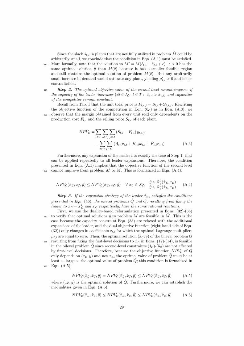
Since the slack st,i in plants that are not fully utilized in problem M could bearbitrarily small, we conclude that the condition in Eqn. (A.1) must be satisfied.More formally, note that the solution to M ′ = M(ct,i − st,i + ε), ε > 0 has the910

same optimal solution y than M(c) because it has a smaller feasible regionand still contains the optimal solution of problem M(c). But any arbitrarilysmall increase in demand would saturate any plant, yielding µ′t,i > 0 and hencecontradiction.

Step 2. The optimal objective value of the second level cannot improve if915

the capacity of the leader increases (∃i ∈ IL, t ∈ T : xt,i > xt,i) and capacitiesof the competitor remain constant.

Recall from Tab. 1 that the unit total price is Pt,i,j = St,i+Gt,i,j . Rewritingthe objective function of the competition in Eqn. (6C) as in Eqn. (A.3), weobserve that the margin obtained from every unit sold only dependents on the920

production cost Ft,i and the selling price St,i of each plant.

NPVC =∑t∈T

∑i∈IC

∑j∈J

(St,i − Ft,i) yt,i,j

−∑t∈T

∑i∈IC

(At,ivt,i +Bt,iwt,i + Et,ixt,i) (A.3)

Furthermore, any expansion of the leader fits exactly the case of Step 1, thatcan be applied repeatedly to all leader expansions. Therefore, the conditionpresented in Eqn. (A.1) implies that the objective function of the second levelcannot improve from problem M to M . This is formalized in Eqn. (A.4).925

NPVC(xL, xC , y) ≤ NPVC(xL, xC , y) ∀ xC ∈ XC ,y ∈ Ψ0

y(xL, xC)y ∈ Ψ0

y(xL, xC)(A.4)

Step 3. If the expansion strategy of the leader xt,i satisfies the conditions

presented in Eqn. (46), the bilevel problems Q and Q, resulting from fixing theleader to xL = xkL and xL respectively, have the same rational reactions.

First, we use the duality-based reformulation presented in Eqns. (32)-(36)to verify that optimal solutions y to problem M are feasible in M . This is the930

case because the capacity constraint Eqn. (33) are relaxed with the additionalexpansions of the leader, and the dual objective function (right-hand side of Eqn.(32)) only changes in coefficients ct,i for which the optimal Lagrange multipliers

µt,i are equal to zero. Then, the optimal solution (xC , y) of the bilevel problem Qresulting from fixing the first-level decisions to xL in Eqns. (12)-(14), is feasible935

in the bilevel problem Q since second-level constraints (1C)-(5C) are not affectedby first-level decisions. Therefore, because the objective function NPVC of Qonly depends on (xC , y) and not xL, the optimal value of problem Q must be atleast as large as the optimal value of problem Q; this condition is formalized inEqn. (A.5).940

NPVC(xL, xC , y) = NPVC(xL, xC , y) ≤ NPVC(xL, xC , y) (A.5)

where (xC , y) is the optimal solution of Q. Furthermore, we can establish theinequalities given in Eqn. (A.6),

NPVC(xL, xC , y) ≤ NPVC(xL, xC , ˆy) ≤ NPVC(xL, xC , y) (A.6)

29

where ˆy is the optimum of Q with xC fixed to xC . The inequality on the left isderived from Eqn. (A.4), and the inequality on the right follows from optimalityof (xC , y) in problem Q. Eqns. (A.5) and (A.6) together demonstrate thatproblems Q and Q have the same optimal objective value that can be givenby the optimal solution (xC , y). We conclude that xL and xL are in the same945

stability region RxL(xC , y), which proves Proposition 6.

References

[1] Ekaterina Alekseeva, Yury Kochetov, and Alexandr Plyasunov. An ExactMethod for the Discrete (r-p)-centroid Problem. Journal of Global Opti-mization, 63:445–460, 2015.950

[2] Natalia Alguacil, Andres Delgadillo, and Jose M. Arroyo. A Trilevel Pro-gramming Approach for Electric Grid Defense Planning. Computers andOperations Research, 41(1):282–290, 2014. ISSN 03050548.

[3] G. Anandalingam and Victor Apprey. Multi-Level Programming and Con-flict Resolution. European Journal of Operational Research, 51(2):233–247,955

1991.

[4] Jonathan F. Bard and James T. Moore. An Algorithm for the DiscreteBilevel Programming Problem. Naval Research Logistics, 39(3):419–435,apr 1992. ISSN 0894069X.

[5] Jonathan F. Bard, John Plummer, and Jean Claude Sourie. A Bilevel Pro-960

gramming Approach to Determining Tax Credits for Biofuel Production.European Journal of Operational Research, 120:30–46, 2000.

[6] Omar Ben-Ayed and Charles E. Blair. Computational Difficulties of BilevelLinear Programming. Operations Research, 38(3):556–560, 1990.

[7] Paul G. Berglund and Changhyun Kwon. Solving a Location Problem of965

a Stackelberg Firm Competing with Cournot-Nash Firms. Networks andSpatial Economics, 14(1):117–132, 2014. ISSN 15729427.

[8] Suk-Gwon Chang and Bezalel Gavish. Telecommunications Network Topo-logical Design and Capacity Expansion: Formulations and Algorithms.Telecommuncation Systems, 1(1):99–131, 1993.970

[9] Andres Delgadillo, Jose Manuel Arroyo, and Natalia Alguacil. Analysisof Electric Grid Interdiction with Line Switching. IEEE Transactions onPower Systems, 25(2):633–641, 2010. ISSN 08858950.

[10] Stephan Dempe. Foundations of Bilevel Programming. Springer Science &Business, 2002.975

[11] Stephan Dempe, Boris S. Mardukhovich, and Alain B. Zemkoho. NecessaryOptimality Conditions in Pessimistic Bilevel Programming. Optimization,63(4):505–533, 2014.

[12] Scott T. DeNegre and Ted K. Ralphs. A Branch-and-Cut Algorithm for In-teger Bilevel Linear Programs. Operations Research and Computer Science980

Interfaces Series, 47:65–78, 2009.

30

[13] Nuno P. Faısca, Vivek Dua, Berc Rustem, Pedro M. Saraiva, and Efstra-tios N. Pistikopoulos. Parametric Global Optimisation for Bilevel Pro-gramming. Journal of Global Optimization, 38(4):609–623, oct 2006. ISSN0925-5001.985

[14] Terry L. Friesz, Matthew A. Rigdon, and Reetabrata Mookherjee. Differ-ential Variational Inequalities and Shipper Dynamic Oligopolistic NetworkCompetition. Transportation Research Part B, 40:480–503, 2006.

[15] Pablo Garcia-Herreros, Lei Zhang, Pratik Misra, Erdem Arslan, SanjayMehta, and Ignacio E. Grossmann. Mixed-Integer Bilevel Optimization990

for Capacity Planning with Rational Markets. Computers and ChemicalEngineering, 86:33–47, 2016.

[16] Fred Glover. Improved Linear Integer Programming Formulations of Non-linear Integer Problems. Management Science, 22(4):455–460, 1975.

[17] Ignacio E. Grossmann. Advances in Mathematical Programming Models995

for Enterprise-Wide Optimization. Computers and Chemical Engineering,47:2–18, 2012.

[18] Zeynep H. Gumus and Christodoulos A. Floudas. Global Optimizationof Mixed-Integer Bilevel Programming Problems. Computational Manage-ment Science, 2(3):181–212, 2005.1000

[19] Louis S. Hakimi. On Locating New Facilities in a Competitive Environment.European Journal of Operational Research, 12(1):29–35, 1983.

[20] Jialin Han, Jie Lu, Yaoguang Hu, and Guangquan Zhang. Tri-levelDecision-Making with Multiple Followers: Model, Algorithm and CaseStudy. Information Sciences, 311:182–204, 2015.1005

[21] Robert G. Jeroslow. The Polynomial Hierarchy and a Simple Model forCompetitive Analysis. Mathematical Programming, 32(2):146–164, 1985.

[22] Athanasia Karakitsiou. Modeling Discrete Competitive Facility Location.Springer, 2015.

[23] Athanasia Karakitsiou and Athanasios Migdalas. Locating Facilities in a1010

Competitive Environment. Optimization Letters, 2015. ISSN 1862-4472.

[24] Polyxeni-M. Kleniati and Claire S. Adjiman. Branch-and-Sandwich: aDeterministic Global Optimization Algorithm for Optimistic Bilevel Pro-gramming Problems. Part II: Convergence Analysis and Numerical Results.Journal of Global Optimization, 60(3):459–481, 2014. ISSN 0925-5001.1015

[25] Dominik Kress and Erwin Pesch. Sequential Competitive Location on Net-works. European Journal of Operational Research, 217:483–499, 2012.

[26] Peter B. Luh, Shi-Chung Chang, and Tsu-Shuan Chang. Solutions andProperties of Multi-stage Stackeiberg Games. Automatica, 20(2):251–256,1984.1020

[27] Athanasios Migdalas. Bilevel Programming in Traffic Planning: Models,Methods and Challenge. Journal of Global Optimization, 7:381–405, 1995.

31

[28] Tan C. Miller, Terry L. Friesz, Roger L. Tobin, and Changhyun Kwon.Reaction Function Based Dynamic Location Modeling in Stackelberg-Nash-Cournot Competition. Networks and Spatial Economics, 7:77–97, 2007.1025

[29] Alexander Mitsos, George M. Bollas, and Paul I. Barton. Bilevel Op-timization Formulation for Parameter Estimation in LiquidLiquid PhaseEquilibrium Problems. Chemical Engineering Science, 64:548–559, 2009.

[30] James T. Moore and Jonathan F. Bard. The Mixed Integer Linear BilevelProgramming Problem. Operations Research, 38(5):911–921, 1990.1030

[31] Frederic H. Murphy and Yves Smeers. Generation Capacity Expansionin Imperfectly Competitive Restructured Electricity Markets. OperationsResearch, 53(4):646–661, 2005. ISSN 0030-364X.

[32] Pierre-Louis Poirion, Sonia Toubaline, Claudia D’ambrosio, and Leo Lib-erti. Bilevel Mixed-Integer Linear Programs and the Zero Forcing Set.1035

optimization-online.org: 5210, 2015.

[33] Marcos Costa Roboredo and Artur Alves Pessoa. A Branch-and-Cut Algo-rithm for the Discrete (r-p)-centroid Problem. European Journal of Oper-ational Research, 224(1):101–109, 2013.

[34] Maria P. Scaparra and Richard L. Church. A Bilevel Mixed-Integer Pro-1040

gram for Critical Infrastructure Protection Planning. Computers & Oper-ations Research, 35(6):1905–1923, 2008.

[35] Hanif D. Sherali, Allen L. Soyster, and Frederic H. Murphy. Stackelberg-Nash-Cournot Equilibria: Characterizations and Computations. Opera-tions Research, 31(2):253–276, 1983.1045

[36] J. Cole Smith, Churluzu Lim, and Aydin Alptekinoglu. Optimal Mixed-Integer Programming and Heuristic Methods for a Bilevel StackelbergProduct Introduction Game. Naval Research Logistics, 56(8):714–729,2009.

[37] Wolfram Wiesemann, Angelos Tsoukalas, and Polyxeni-Margarita Kleniati.1050

Pessimistic Bilevel Optimization. SIAM Journal on Optimization, 23(1):353–380, 2013.

[38] Pan Xu and Lizhi Wang. An Exact Algorithm for the Bilevel Mixed Inte-ger Linear Programming Problem under Three Simplifying Assumptions.Computers and Operations Research, 41:309–318, 2014. ISSN 03050548.1055

[39] Yiming Yao, Thomas Edmunds, Dimitri Papageorgiou, and Rogelio Al-varez. Trilevel Optimization in Power Network Defense. IEEE Transac-tions on Systems, Man and Cybernetics Part C: Applications and Reviews,37(4):712–718, 2007. ISSN 10946977.

[40] Alain B. Zemkoho. Solving Ill-posed Bilevel Programs. Set-Valued and1060

Variational Analysis, 24(3):423–448, 2016.

[41] Bo Zeng. Easier than We Thought : A Practical Scheme to ComputePessimistic Bilevel Optimization Problem. Available at SSRN 2658342,2015.

32

[42] Bo Zeng and Yu An. Solving Bilevel Mixed Integer Program by Reformu-1065

lations and Decomposition. Optimization On-line, 2014.

33