LONG MEMORY IN CONTINUOUS-TIME STOCHASTIC … · Mathematical Finance, Vol. 8, No. 4 (October 1998), 291–323 LONG MEMORY IN CONTINUOUS-TIME STOCHASTIC VOLATILITY MODELS FABIENNE

Mathematical Finance, Vol. 8, No. 4 (October 1998), 291–323

LONG MEMORY IN CONTINUOUS-TIME STOCHASTICVOLATILITY MODELS

FABIENNE COMTE

URA 1321 and LSTA, University Paris 6 and CREST-ENSAE

ERIC RENAULT

GREMAQ-IDEI, University of Toulouse and Institut Universitaire de France

This paper studies a classical extension of the Black and Scholes model for option pricing, oftenknown as the Hull and White model. Our specification is that the volatility process is assumed not onlyto be stochastic, but also to have long-memory features and properties. We study here the implicationsof this continuous-time long-memory model, both for the volatility process itself as well as for theglobal asset price process. We also compare our model with some discrete time approximations. Thenthe issue of option pricing is addressed by looking at theoretical formulas and properties of the implicitvolatilities as well as statistical inference tractability. Lastly, we provide a few simulation experimentsto illustrate our results.

KEY WORDS: continuous-time option pricing model, stochastic volatility, volatility smile, volatilitypersistence, long memory

1. INTRODUCTION

If option prices in the market were conformable with the Black–Scholes (1973) formula,all the Black–Scholes implied volatilities corresponding to various options written on thesame asset would coincide with the volatility parameterσ of the underlying asset. In realitythis is not the case, and the Black–Scholes (BS) implied volatilityσ

impt,T heavily depends

on the calendar timet , the time to maturityT − t , and the moneyness of the option. Thismay produce various biases in option pricing or hedging when BS implied volatilities areused to evaluate new options or hedging ratios. These price distortions, well-known topractitioners, are usually documented in the empirical literature under the terminology ofthe smile effect, where the so-called “smile” refers to the U-shaped pattern of impliedvolatilities across different strike prices.

It is widely believed that volatility smiles can be explained to a great extent by a modelingof stochastic volatility, which could take into account not only the so-called volatilityclustering (i.e., bunching of high and low volatility episodes) but also the volatility effectsof exogenous arrivals of information. This is why Hull and White (1987), Scott (1987), andMelino and Turnbull (1990) have proposed an option pricing model in which the volatilityof the underlying asset appears not only time-varying but also associated with a specific

A previous version of this paper has benefitted from helpful comments from S. Pliska, L. C. G. Rogers, M. Taqqu,and two anonymous referees. All remaining errors are ours.

Initial manuscript received December 1995; final revision received September 1997.Address correspondence to F. Comte, ISUP Boite 157, Universit´e Paris 6, 4 Place Jussieu, 75 252 Paris cedex

05 France; e-mail: [email protected].

c© 1998 Blackwell Publishers, 350 Main St., Malden, MA 02148, USA, and 108 Cowley Road, Oxford,OX4 1JF, UK.

291

292 FABIENNE COMTE AND ERIC RENAULT

risk according to the “stochastic volatility” (SV) paradigm

{ dS(t)S(t) = µ(t, S(t))dt + σ(t)dw1(t)

d(ln σ(t)) = k(θ − ln σ(t))dt + γdw2(t),(1.1)

whereS(t) denotes the price of the underlying asset,σ(t) is its instantaneous volatility, and(w1(t), w2(t)) is a nondegenerate bivariate Brownian process. The nondegenerate featureof (w1, w2) is characteristic of the SV paradigm, in contrast to continuous-time ARCH-type models where the volatility process is a deterministic function of past values of theunderlying asset price.

The logarithm of the volatility is assumed to follow an Ornstein–Uhlenbeck process,which ensures that the instantaneous volatility process is stationary, a natural way to gener-alize the constant-volatility Black and Scholes model. Indeed, any positive-valued station-ary process could be used as a model of the stochastic instantaneous volatility (see Ghysels,Harvey and Renault (1996) for a review). Of course, the choice of a given statistical modelfor the volatility process heavily influences the deduced option pricing formula. More pre-cisely, Hull and White (1987) show that, under specific assumptions, the price at timet ofa European option of exercise dateT is the expectation of the Black and Scholes optionpricing formula where the constant volatilityσ is replaced by its quadratic average over theperiod:

σ 2t,T =

1

T − t

∫ T

tσ 2(u)du,(1.2)

and where the expectation is computed with respect to the conditional probability distri-bution ofσ 2

t,T givenσ(t). In other words, the square of implied Black–Scholes volatility

σimpt,T appears to be a forecast of the temporal aggregationσ 2

t,T of the instantaneous volatilityviewed as a flow variable.

It is now well known that such a model is able to reproduce some empirical stylizedfacts regarding derivative securities and implied volatilities. A symmetric smile is wellexplained by this option pricing model with the additional assumption of independencebetweenw1 andw2 (see Renault and Touzi (1996)). Skewness may explain the correlationof the volatility process with the price process innovations, the so-called leverage effect(see Hull and White 1987). Moreover, a striking empirical regularity that emerges fromnumerous studies is the decreasing amplitude of the smile being a function of time tomaturity; for short maturities the smile effect is very pronounced (BS implied volatilitiesfor synchronous option prices may vary between 15% and 25%), but it almost completelydisappears for longer maturities. This is conformable to a formula like (1.2) because itshows that, when time to maturity is increased, temporal aggregation of volatilities erasesconditional heteroskedasticity, which decreases the smile phenomenon.

The main goal of the present paper is to extend the SV option pricing model in orderto capture well-documented evidence ofvolatility persistenceand particularly occurrenceof fairly pronounced smile effects even for rather long maturity options. In practice, thedecrease of the smile amplitude when time to maturity increases turns out to be muchslower than it goes according to the standard SV option pricing model in the setting (1.1).This evidence is clearly related to the so-called volatility persistence, which implies thattemporal aggregation (1.2) is not able to fully erase conditional heteroskedasticity.

Generally speaking, there is widespread evidence that volatility is highly persistent.

LONG MEMORY IN CONTINUOUS-TIME STOCHASTIC VOLATILITY MODELS 293

Particularly for high frequency data one finds evidence of near unit root behavior of theconditional variance process. In the ARCH literature, numerous estimates of GARCHmodels for stock market, commodities, foreign exchange, and other asset price series areconsistent with an IGARCH specification. Likewise, estimation of stochastic volatilitymodels show similar patterns of persistence (see, e.g., Jacquier, Polson and Rossi 1994).These findings have led to a debate regarding modeling persistence in the conditionalvariance process either via a unit root or a long memory-process. The latter approach hasbeen suggested both for ARCH and SV models; see Baillie, Bollerslev, and Mikkelsen(1996), Breidt, Crato, and De Lima (1993), and Harvey (1993). This allows one to considermean-reverting processes of stochastic volatility rather than the extreme behavior of theIGARCH process which, as noticed by Baillie et al. (1996), has low attractiveness for assetpricing since “the occurence of a shock to the IGARCH volatility process will persist foran infinite prediction horizon.”

The main contribution of the present paper is to introduce long-memory mean revertingvolatility processes in the continuous time Hull and White setting. This is particularlyattractive for option pricing and hedging through the so-calledterm structure of BS impliedvolatilities (see Heynen, Kemna, and Vorst 1994). More precisely, the long-memory featureallows one to capture the well-documented evidence of persistence of the stochastic featureof BS implied volatilities, when time to maturity increases. Since, according to (1.2), BSimplied volatilities are seen as an average of expected instantaneous volatilities in the sameway that long-term interest rates are seen as average of expected short rates, the type ofphenomenon we study here is analogous to the studies by Backus and Zin (1993) and Comteand Renault (1996) who capture persistence of the stochastic feature of long-term interestrates by using long-memory models of short-term interest rates.

Indeed, we are able to extend Hull and White option pricing to a continuous-time long-memory model of stochastic volatility by replacing the Wiener processw2 in (1.1) bya fractional Brownian motionw2

α, with α restricted to 0≤ α < 12 (instead of|α| <

12 allowed by the general definition because long memory occurs on that range only).Note that the Wiener case corresponds toα = 0. Of course, for nonzeroα, w2

α is nolonger a semimartingale (see Rogers 1995), and thus usual stochastic integration theoryis not available. But, following Comte and Renault (1996), we only needL2 theory ofintegration for Gaussian processes and we obtain option prices that, although they arefunctions of the underlying volatility processes, do ensure the semimartingale property as amaintained hypothesis for asset price processes (including options).1 This semimartingaleproperty is all the more important for asset prices processes because stochastic processesthat are not semimartingales do not admit equivalent martingale measures. Indeed we knowfrom Delbaen and Schachermayer (1994) that an asset price process admits an equivalentmartingale measure if and only if the NFLVR (no free lunch with vanishing risk) conditionholds. As stressed by Rogers (1995), when this condition fails, “this does not of itselfimply the existence of arbitrage, though in any meaningful economic sense it is just asbad as that.” In that event, Rogers (1995) provides a direct construction of arbitrage withfractional Brownian motion. As long as the volatility itself is not a traded asset, all asset priceprocesses that we consider here (underlying asset and options written on it) are conformable

1We are very grateful to L. C. G. Rogers to have helped us, in a private communication, to check this point. Thesemimartingale property of an option priceCt comes from the fact that it is computed as a conditional expectation

of a (nonlinear) function of∫ T

tσ 2(u)du. This integration reestablishes the semimartingale property that was lost

by the volatility process itself.


to the NFLVR. Note that we have nevertheless the same usual problem as in all models ofthat kind: the nonuniqueness of the neutral-risk equivalent measure.

The paper is organized as follows. We study in Section 2 the probabilistic properties ofour Fractional Stochastic Volatility (FSV) model in continuous time, obtained by replacingthe Wiener processw2 in (1.1) by the following process that may be seen as a truncatedversion of the general fractional Brownian motion2:

w2α(t) =

∫ t

0

(t − s)α

0(1+ α) dw2(s), 0< α <1

2.

We explain why a high degree of fractional differencingα allows one to take into account theapparent widespread finding of integrated volatility for high frequency data. Section 3 givesthe basis for more empirical studies of our FSV model through discrete time approximations.We stress the advantages of continuous-time modeling of long memory with respect to theusual ARFIMAa la Geweke and Porter-Hudak (1983) or their FIGARCH analogue in theARCH literature. The main point is that only a continuous-time definition of the parametersof interest allows one to clearly disentangle long-memory parameters from short-memoryones.

Section 4 is devoted to the issue of option pricing and the study of the properties andfeatures of implied volatilities. Since the first equation of (1.1) has remained invariant byour long-memory generalization of the Hull and White (1987) option pricing model, theirargument can be extended in order to set an option pricing formula. The only change isthe law of motion of the instantaneous volatility, whose long-memory feature modifies theorders of conditional heteroskedasticity (forecasted, temporally aggregated,. . . ) and ofkurtosis coefficients with respect to time to maturity. We derive some formulas about theseorders which extend those of Drost and Werker (1996) and thus “close the FIGARCH gap.”

The statistical inference issue is addressed in Section 5. Of course, if the instantaneousvolatility σ(t) were observed, Comte and Renault’s (1996) work about the estimation ofcontinuous-time long-memory models could be used. But instantaneous volatilities are notdirectly observed and can only be filtered, either by an extension to FIGARCH models ofNelson and Foster’s (1994) methodology or by using option prices as Pastorello, Renault,and Touzi (1993) do in the Hull and White context. Note that forα 6= 0 the volatility processis no longer Markovian, so this may make awkward the practical use of the Hull and Whiteoption pricing formula. Nevertheless, it is shown how one could extend the Pastorello etal. (1993) methodology to the present framework. The alternative methodology we suggestin the present paper is to use approximate discretizations of theS(t) stock price processin order to obtain some proxies of instantaneous volatilities and work with approximatelikelihoods.

The discretizations found in Section 3 are used in Section 6 to perform some simulationexperiments about continuous-time FSV models. A descriptive study of the resulting pathscan then be obtained. The estimation procedures are compared through these Monte Carloexperiments. The misspecification bias introduced by a FIGARCH approximation of ourcontinuous-time models is documented.

2This process is a tool for easyL2 definitions of integrals w.r.t. the Fractional Brownian Motion (FBM), but

can be replaced by the true FBM∫ 0

−∞((t − s)α − (−s)α)dw2(s)+ w2α(t).


2. THE FRACTIONAL STOCHASTIC VOLATILITY MODEL

2.1. A Simple Fractional Long-Memory Process

Comte and Renault (1996) used fractional processes to generalize the notion of StochasticDifferential Equation (SDE) of orderp. We consider here only the first-order fractionalSDE:

dx(t) = −kx(t)dt + σdwα(t), x(0) = 0, k > 0, 0< α <1

2.(2.1)

The solution can be written (see Comte and Renault 1996) asx(t) = ∫ t0 e−k(t−s)σ dwα(s).

Integration with respect towα is defined only in the WienerL2 sense and for the integrationof deterministic functions only. We thus obtain families of Gaussian processes. The processx(t) also can be written as

∫ t0 a(t − s)dw(s) with

a(x) = σ

0(1+ α)d

dx

∫ x

0e−ku(x − u)α du(2.2)

= σ

0(1+ α)(

xα − ke−kx∫ x

0ekuuα du

).

We denote byy(t) the “stationary version” ofx(t), y(t) = ∫ t−∞ a(t − s)dw(s). Therefore,

the solutionx of the fractional SDE is given by

x(t) =∫ t

0

(t − s)α

0(1+ α) dx(α)(s),(2.3)

where its derivative of orderα is the solution

x(α)(t) = d

dt

∫ t

0

(t − s)−α

0(1− α) =∫ t

0e−k(t−s)σ dw(s)(2.4)

of the associated standard SDE.We can also give the general (continuous-time) spectral density of processes that are

solutions of (2.1):

f c(λ) = σ 2

0(1+ α)2λ2α

1

λ2+ k2.(2.5)

Lastly, it seems interesting to note that long-memory fractional processes as considered inComte and Renault (1996) and solutions of (2.1) in particular have the following propertiesproved in Comte (1996):

i. The covariance functionγ = γy associated withx satisfies forh → 0 andψconstant:

γ (h) = γ (0)+ 1

2ψ.|h|2α+1+ o(|h|2α+1).(2.6)


ii. x is ergodic in theL2 sense:1T

∫ T0 x(s)ds

m.s.−→T→+∞

0.

iii. There is a processz(t) equivalent3 to x(t) and such that the sample function ofzsatisfies a Lipschitz condition of orderβ, ∀β ∈ (0, α + 1

2), a.s.

Thus the greater the value ofα, the smoother the path of the process.

2.2. Properties of the Volatility in the FSV Model

The basic idea of our modeling strategy (see (1.1)) is to assume that the logarithmx(t) = ln σ(t) of the stochastic volatility is a solution of the first-order SDE (2.1). For thesake of simplicity, we assumeθ = 0 since it does not change the probabilistic propertiesof the process. Thus the volatility processσ(t) is asymptotically equivalent (in quadraticmean) to the stationary process:

σ (t) = exp

(∫ t

−∞e−k(t−s)γdw2

α(s)

), k > 0, 0< α <

1

2.(2.7)

As in usual diffusion models of stochastic volatility, the volatility process is assumed tobe asymptotically stationary and nowhere differentiable. This is the reason we do not usean SDE (even fractional) of higher order. Nevertheless, the fractional exponentα providessome degree of freedom in the order of regularity. Indeed, it is possible to show forσ(t)the same type of regularity property as for the fractional processx(t) = ln σ(t).

PROPOSITION2.1. Let rσ (h) = cov(σ (t + h), σ (t)), whereσ is given by (2.7). Then,for h→ 0, rσ (h) = rσ (0)+ η.|h|2α+1+ o(|h|2α+1), whereη is a given constant.

(See Appendix A for all proofs.)Roughly speaking, the autocorrelation function of the stationary processσ fulfills the

regularity condition that ensures the Lipschitz feature of the sample paths. The greaterα

is, the smoother the path of the volatility process is. Therefore, a high degree of fractionaldifferencingα allows one to take into account the apparent widespread finding of integratedvolatility for high frequency data (see the simulation in Section 6.2). As a matter of fact,we can see that

α > 0⇒ rσ (h)− rσ (0)

h−→h→0

0,

which could be interpreted as a near-integrated behavior

rσ (h)− rσ (0)

h= ρh − 1

h−→h→0

ln ρ−→ρ→1

0

if σ(t) is considered as a continuous-time AR(1) process with a correlation coefficientρ

near 1.

3Two processes are called equivalent if they coincide almost surely.


This analogy between a unit root hypothesis and its fractional alternatives has alreadybeen used for unit root tests by Robinson (1993). Robinson’s methodology could be a usefultool for testing integrated volatility against long memory in stochastic volatility behavior.

The concept of persistence that we advance thanks to the fractional framework is thatof long memory instead of indefinite persistence of shocks as in the IGARCH framework.Indeed, we can prove the following result:

PROPOSITION2.2. In the context of Proposition 2.1, we have

(i) rσ (h) is of order O(|h|2α−1) for h→+∞.(ii) lim λ→0 λ

2α fσ (λ) = c ∈ R+, where fσ (λ) =∫R rσ (h)eiλh dh is the spectral density

of σ .

Proposition 2.2 illustrates that the volatility process itself (and not only its logarithm) doesentail the long-memory properties (generally summarized as in (i) and (ii) by the behaviorof the covariance function near infinity and of the spectral density near zero) we couldexpect in the FSV model.

3. DISCRETE APPROXIMATIONS OF THE FSV MODEL

3.1. The Volatility Process

The volatility process dynamics are characterized by the fact thatx(t) = ln σ(t) is asolution of the fractional SDE (2.1). So we know two integral expressions forx(t) (withthe notations of Section 2.1):

x(t) =∫ t

0

(t − s)α

0(1+ α) dx(α)(s) =∫ t

0a(t − s) dw2(s),

wherea(t − s) is given by (2.2).A discrete time approximation of the volatility process is a formula to numerically eval-

uate these integrals using only the values of the involved processesx(α)(s) andw2(s) ona discrete partition of [0, t ]: j/n, j = 0,1, . . . , [nt].4 A natural way to obtain suchapproximations (see Comte 1996) is to approximate the integrands by step functions:

xn,1(t) =∫ t

0

(t − [ns]

n

)α0(1+ α) dx(α)(s) and xn,2(t) =

∫ t

0a

(t − [ns]

n

)dw2(s),(3.1)

which gives, neglecting the last terms for large values ofn,

xn(t) =[nt]∑j=1

(t − j−1

n

)α0(1+ α) 1x(α)

(j

n

)and(3.2)

xn(t) =[nt]∑j=1

a

(t − j − 1

n

)1w2

(j

n

),

4[z] is the integerk such thatk ≤ z< k+ 1.


where we use the following notations:1x(α)( jn ) = x(α)( j

n )− x(α)( j−1n ) and 1w2(

jn ) =

w2(jn )− w2(

j−1n ).

Indeed, all these approximations converge toward thex process in distribution in the senseof convergence in distribution for stochastic processes as defined in Billingsley (1968); this

convergence is denoted byD⇒. This result is proved in Comte (1996).

PROPOSITION3.1. xn,1D⇒ x, xn,2

D⇒ x, xnD⇒ x, and xn

D⇒ x when n goes toinfinity.

The proxyxn is the most useful for comparing our FSV model with the standard discretetime models of conditional heteroskedasticity, whereas the most tractable for mathematicalwork is xn.

3.2. FSV versus FIGARCH

Expression (3.2) provides a proxyxn of x in function of the processx(α)( jn ), j =

0,1, . . . , [nt], which is an AR(1) process associated with an innovation processu( jn ), j =

0,1, . . . , [nt]. Let us denote by

(1− ρnLn)x(α)

(j

n

)= u

(j

n

)(3.3)

the representation of this process, whereLn is the lag operator corresponding to the samplingschemej

n , j = 0,1, . . ., LnY( jn ) = Y( j−1

n ), andρn = e−k/n is the correlation coefficientfor the time interval1n .

Since the processx(α) is asymptotically stationary, we can assume without loss of gen-erality that its initial value is zero,x(α)( j

n ) = 0 for j ≤ 0, which of course impliesu( j

n ) = 0 for j ≤ 0. Then we can write

xn

(j

n

)=

j∑i=1

( j − i + 1)α

nα0(1+ α)[

x(α)(

i

n

)− x(α)

(i − 1

n

)]

=[

j−1∑i=0

(i + 1)α − i α

nα0(1+ α) Lin

]x(α)

(j

n

).

Thus,

xn(j

n) =

[j−1∑i=0

(i + 1)α − i α

nα0(1+ α) Lin

](1− ρnLn)

−1u

(j

n

).(3.4)

Expression (3.4) gives a parameterization of the volatility dynamics in two parts: a long-memory part that corresponds to the filter

∑+∞i=0 ai Li

n/nα with ai = ((i+1)α−i α)/0(1+α)and a short-memory part that is characterized by the AR(1) process:(1− ρnLn)

−1u( jn ).

We can show that the long-memory filter is “long-term equivalent” to the usual discretetime long-memory filter(1− L)−α =∑+∞i=0 bi Li , wherebi = 0(i + α)/(0(i + 1)0(α)),


in the sense that there is a long-term relationship (a cointegration relation) between thetwo types of processes. Indeed, we can show (see Comte 1996) that the two long-memoryprocesses,Yt =

∑+∞i=0 ai ut−i andZt =

∑+∞i=0 bi ut−i ,whereai andbi are defined previously

andut is any short-term memory stationary process, are cointegrated:Yt − Zt is shortmemory and

∑+∞i=0 |ai − bi | < +∞, whereas

∑+∞i=0 ai =

∑+∞i=0 bi = +∞.

But this long-term equivalence between our long-memory filter and the usual discretetime one(1− L)−α does not imply that the standard parameterization ARFIMA(1, α,0)is well-suited in our framework. Indeed, short-memory characteristics may be hiddenby the short-term difference between the two filters. In other words, not only(1− ρnLn)(n(1− Ln))

α xn(jn ) is not in general a white noise,5 but we are not even sure that

(n(1− Ln))α xn

(jn

)is an AR(1) process (even though we know that it is a short-memory

stationary process). The usual discrete time filter(1−L)α introduces some mixing betweenlong- and short-term characteristics (see Comte 1996 and Section 6.3 for illustration).

This is the first reason why we believe that the FSV model is more relevant for high-frequency data than the FIGARCH model since the latter is based on an ARFIMA modelingof the squared innovations (see Baillie et al. 1996). The second reason is that the FSV modelrepresents the log-volatility as an “AR(1) long-memory” process with a specific risk (in theparticular caseα = 0, (3.4) corresponds to the stochastic variance model of Harvey, Ruiz,and Shephard 1994), but the GARCH type modeling does not introduce an exogenous riskof volatility and, by the way, does not explain why option markets are useful to hedge aspecific risk.

3.3. The Global Filtering Model

In order to obtain a complete discrete time approximation of our FSV model, we haveto discretize not only the volatility process, but also the associated asset price processS(t)according to (1.1). Since it is not difficult to compute some discretizations of the trend partof an SDE, we can assume in this subsection, for the sake of notational simplicity, that lnS(t)is a martingale. Not only are we always able to perform a preliminary centering of the priceprocess in order to be in this case, but also it is well known that the martingale hypothesisis often directly accepted, for exchange rates for example. So, withY(t) = ln S(t) we areinterested in the following dynamics:

{dY(t) = σ(t)dw1(t)d(ln σ(t)) = −k ln σ(t)dt + γdw2

α(t).(3.5)

For a known processσ , a discretized approximationYn of the processY can directly beobtained by a way similar to (3.1):

Yn(t) =∫ t

0σ

([ns]

n

)dw1(s)

=[nt]∑j=1

σ

(j − 1

n

)1w1

(j

n

)+ σ

([nt]

n

)(w1(t)− w1

([nt]

n

)).

5The fractional differencing operator(1 − L)α has to be modified into(n(1 − Ln))α in order to correctly

normalize the unit root with respect to the unit period of time.


Andbya remarkof thesame typeas (3.2), wecanalsoconsiderYn(t)=∑[nt]

j=1σ(j−1n )1w1(

jn ).

It can be proved that:

LEMMA 3.1. YnD⇒ Y andYn

D⇒ Y , when n grows to infinity.

But from a practical viewpoint, the discretizationsYn andYn are not very useful becausethey are based on the values of the processσ , which cannot be computed without some othererrors of discretization. Thus we are more interested in the following joint discretization:

σn(t) = exp

[[nt]∑j=1

a

(t − j − 1

n

)1w2

(j

n

)],(3.6)

Yn(t) =[nt]∑j=1

σn

(j − 1

n

)1w1

(j

n

).

We can then prove the following proposition.

PROPOSITION3.2.

(Yn

σn

)D⇒(

Yσ

)and thus

(Sn = ln Yn

σn

)D⇒(

Sσ

)when n→∞.

Another parameterization can be obtained by usingσn(t) = exp(xn(t)) rather thanσn(t) = exp(xn(t)); the previous section has shown how this parameterization is givenby α andρn.

We have something like a discrete time stochastic variance model `a la Harvey et al. (1994)which converges toward our FSV model when the sampling interval1

n converges towardzero. The only difference is that, whenα 6= 0, ln σn(t) is not an AR(1) process but a long-memory stationary process. Such a generalization has in fact been considered in discretetime by Harvey (1993) in a recent working paper. He works withyt = σtεt , εt ∼ I I D (0,1),t = 1, . . . , T , σ 2

t = σ 2 exp(ht ), (1− L)dht = ηt , ηt ∼ I I D (0, σ 2η ), 0 ≤ d ≤ 1. The

analogy with (3.6) is then obvious, with the remaining problem being the choice of the rightapproximation of the fractional derivation studied in the previous subsection. Moreover,our case is a little different from the one studied by Harvey in that we have in mind avolatility process of the type ARFIMA(1, α,0) where he has an ARFIMA(0,d,0). Butsuch discrete time models may be also useful for statistical inference.

4. OPTION PRICING AND IMPLIED VOLATILITIES

4.1. Option Pricing

The maintained assumption of our option pricing model is characterized by the pricemodel (1.2), where(w1(t), w2(t)) is a standard Brownian motion. Let(Ä,F,P) bethe fundamental probability space.(Ft )t∈[0,T ] denotes theP-augmentation of the filtra-tion generated by(w1(τ ), w2(τ )), τ ≤ t . It coincides with the filtration generated by(S(τ ), σ (τ )), τ ≤ t or (S(τ ), x(α)(τ )), τ ≤ t , with x(t) = ln σ(t).

We look here for the call option premiumCt , which is the price at timet ≤ T of aEuropean call option on the financial asset of priceSt at t , with strike K and maturing at


time T . The asset is assumed not to pay dividends, and there are no transaction costs.Let us assume that the instantaneous interest rate at timet , r (t), is deterministic, so that

the price at timet of a zero coupon bond of maturityT is B(t, T) = exp(− ∫ Tt r (u)du).

We know from Harrison and Kreps (1981) that the no free lunch assumption is equivalentto the existence of a probability distributionQ on (Ä,F), equivalent toP, under which thediscountedprice processesare martingales. We emphasize that no change of probability ofthe Girsanov type could have transformed the volatility process into a martingale, but thereis no such problem for the price processS(t). This stresses the interest of such modelswhere the nonstandard fractional properties are set onσ(t) and not directly onS(t). Thisavoids any of the possible problems of stochastic integration with respect to a fractionalprocess, which does not admit any standard decomposition. Indeed, theσ process appearsonly as a predictible and evenL2 continuous integrand.

Then we can use the standard arguments. An equivalent measureQ is characterized by acontinuous version of the density process ofQ with respect toP (see Karatzas and Shreve1991, p. 184):

M(t) = exp

(−∫ t

0λ(u)′dW(u)− 1

2

∫ t

0λ(u)′λ(u)du

),

whereW = (w1, w2)′ andλ = (λ1, λ2)′ is adapted to{Ft } and satisfies the integrability

condition∫ T

0 λ(u)′λ(u)du < ∞ a.s. The processesλ1 andλ2 can be considered as risk

premia relative to the two sources of riskw1 andw2. Moreover, the martingale propertyunderQ of the discounted asset prices implies that:λ1(t)σ (t) = µ(t, S(t))− r (t).

As the market is incomplete, as is usual in such a context (two sources of risk and onlyone risky asset traded), there is no such relation fixing the volatility risk premiumλ2 and,indeed, the martingale probabilityQ is not unique.

We need to restrict the set of equivalent martingale probabilities by assuming that theprocessλ2(t) is a deterministic functionλ2 of the two argumentst andσ(t):

(A) λ2(t) = λ2(t, σ (t)), ∀t ∈ [0, T ],

which is a common assumption.Girsanov’s theorem leads to a characterization of the distribution underQ of the under-

lying asset. Let:

w1(t) = w1(t)+∫ t

0λ1(u)du and w2(t) = w2(t)+

∫ t

0λ2(u)du.

Then(w1, w2) = w′ is a two-dimensional standardQ-Wiener process adapted to{Ft }. Inparticular,w1 andw2 are independent underQ by construction. Moreoverσ is the solutionto an equation depending only onw2 that can be rewritten as a stochastic differential equationin w2 (depending also onλ2). Thus the processesw1 andσ are still independent underQ.With Q defined as previously, the call option price is given by

Ct = B(t, T)EQ[Max(0, ST − K ) | Ft ],(4.1)


whereEQ(. | Ft ) is the conditional expectation operator, givenFt , when the price dynamicsis governed byQ. Sincew1 andσ are independent underQ, theQ distribution of ln(ST/St )

given byd ln St = (r (t)−(σ (t)2/2)dt+σ(t)dw1(t) conditionally on bothFt and the wholevolatility path(σ (t))t∈[0,T ] is Gaussian with mean

∫ Tt r (u)du− 1

2

∫ Tt σ(u)

2du and variance∫ Tt σ(u)

2du. Therefore, computing the expectation (4.1) conditionally on the volatilitypath gives:

Ct = S(t)

{EQ

t

[8

(mt

Ut,T+ Ut,T

2

)∣∣∣∣Ft

]− e−mtEQ

t

[8

(mt

Ut,T− Ut,T

2

)∣∣∣∣Ft

]},(4.2)

wheremt = ln(

S(t)K B(t,T)

), Ut,T =

√∫ Tt σ(u)

2 du, and8(u) = 1√2π

∫ u−∞ e−t2/2 dt.

The dynamics ofσ are now given by

lnσ(t)

σ (0)=(−k

∫ t

0ln σ(u) du− γ

∫ t

0

(t − s)α

0(1+ α)λ2(s)ds

)+ γ w2

α(t),

where

w2α(t) =

∫ t

0

(t − s)α

0(1+ α) dw2(s).

Then differentiatingx(t) = ln σ(t) with fractional orderα gives:

dx(α)(t) = (−kx(α)(t)+ γ λ2(t))dt + γdw2(t),(4.3)

where

x(α)(t) = d

dt

∫ t

0

(t − s)−α

0(1− α) x(s) ds

is the derivative of (fractional) orderα of x.We can give the general solution of (4.3):

x(α)(t) =(

c+∫ t

0γeksλ2(s)ds+

∫ t

0γeksdw2(s)

)e−kt

and deducex by fractional integration.As usual, when one wants to perform statistical inference using arbitrage pricing models,

two approaches can be imagined: either specify a given parametric form of the risk premiumor assume that the associated risk is not compensated. When trading of volatility is observedit might be relevant to assume a risk premium on it. But we choose here, for the sake ofsimplicity (see, e.g., Engle and Mustafa 1992 or Pastorello et al. 1993 for similar strategiesin short-memory settings) to assume that the volatility risk is not compensated, i.e., thatλ2 = 0. Under this simplifying assumption, which has some microeconomics foundations(see Pham and Touzi 1996), the probability distributions ofUt,T are the same underP andunderQ. In other words the expectation operator in the option pricing formula (4.2) can beconsidered with respect toP.


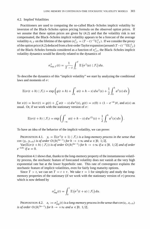
4.2. Implied Volatilities

Practitioners are used to computing the so-called Black–Scholes implicit volatility byinversion of the Black–Scholes option pricing formula on the observed option prices. Ifwe assume that these option prices are given by (4.2) and that the volatility risk is notcompensated, the Black–Scholes implicit volatility appears to be a forecast of the averagevolatility σt,T on the lifetime of the option(σ 2

t,T = (T− t)−1U2t,T ). If we consider the proxy

of the option price (4.2) deduced from a first-order Taylor expansion (around(T−t)−1EU2t,T )

of the Black–Scholes formula considered as a function ofσ 2t,T , the Black–Scholes implicit

volatility dynamics would be directly related to the dynamics of

σ 2imp,T (t) =

1

T − t

∫ T

tE(σ 2(u) | Ft

)du.

To describe the dynamics of this “implicit volatility” we start by analyzing the conditionallaws and moments ofσ :

E(σ (t + h) | Ft ) = exp

(g(t + h)+

∫ t

0a(t + h− s)dw2(s)+ 1

2

∫ h

0a2(x)dx

)

for x(t) = ln σ(t) = g(t) + ∫ t0 a(t − s)dw2(s), g(t) = x(0) + (1− e−kt)θ , anda(x) as

usual. Or, if we work with the stationary version ofσ :

E(σ (t + h) | Ft ) = exp

(∫ t

−∞a(t + h− s)dw(2)(s)+ 1

2

∫ h

0a2(x)dx

).

To have an idea of the behavior of the implicit volatility, we can prove:

PROPOSITION4.1. yt = E(σ 2(t + 1) | Ft ) is a long-memory process in the sense thatcov (yt , yt+h) is of order O(|h|2α−1) for h→+∞ andα ∈ ]0, 1/2[.

Var(E(σ (t + h) | Ft )) is of order O(|h|2α−1) for h→+∞ if α ∈ ]0, 1/2[ and of ordere−k|h| if α = 0.

Proposition 4.1 shows that, thanks to the long-memory property of the instantaneous volatil-ity process, the stochastic feature of forecasted volatility does not vanish at the very highexponential rate but at the lower hyperbolic rate. This rate of convergence explains thestochastic feature of implicit volatilities, even for fairly long maturity options.

SinceT > t , we can setT = t + τ . We takeτ = 1 for simplicity and study the long-memory properties of the stationary (if we work with the stationary version ofσ ) processwhich is now defined by

σ 2imp(t) =

∫ 1

0E(σ 2(t + u) | Ft

)du.

PROPOSITION4.2. zt := σ 2imp(t) is a long-memory process in the sense thatcov(zt , zt+h)

is of order O(|h|2α−1) for h→+∞ andα ∈ ]0, 1/2[.


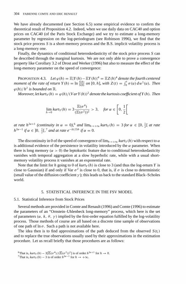
We have already documented (see Section 6.5) some empirical evidence to confirm thetheoretical result of Proposition 4.2. Indeed, when we use daily data on CAC40 and optionprices on CAC40 (of the Paris Stock Exchange) and we try to estimate a long-memoryparameter by regression on the log-periodogram (see Robinson 1996), we find that thestock price processS is a short-memory process and the B.S. implicit volatility process isa long-memory one.

Finally, the dynamics of conditional heteroskedasticity of the stock price processS canbe described through the marginal kurtosis. We are not only able to prove a convergenceproperty like Corollary 3.2 of Drost and Werker (1996) but also to measure the effect of thelong-memory parameter on the speed of convergence:

PROPOSITION4.3. Letϕ(h) = E|Y(h)−EY(h)|4 = EZ(h)4 denote the fourth centeredmoment of the rate of return Y(h) = ln S(h)

S(0) on [0, h], with Z(t) = ∫ t0 σ(u)dw1(u). Then

ϕ(h)/h2 is bounded onR.Moreover, let kurtY(h) = ϕ(h)/(V arY(h))2 denote the kurtosis coefficient of Y(h). Then

limh→0

kurtY(h) = 3E(σ 4)

(E(σ 2))2> 3, for α ∈

[0,

1

2

[

at rate h2α+1 (continuity inα = 0),6 and limh→+∞ kurtY(h) = 3 for α ∈ [0, 12[ at rate

h2α−1 if α ∈ ]0, 12[,7 and at rate e−(k/2)h if α = 0.

The discontinuity in 0 of the speed of convergence of limh→+∞ kurtY(h)with respect toαis additional evidence of the persistence in volatility introduced by theα parameter. Whenthere is long memory(α > 0) the leptokurtic feature due to conditional heteroskedasticityvanishes with temporal aggregation at a slow hyperbolic rate, while with a usual short-memory volatility process it vanishes at an exponential rate.

Note that the limit forh going to 0 ofkurtY(h) is close to 3 (and thus the log-returnY isclose to Gaussian) if and only if Varσ 2 is close to 0, that is, ifσ is close to deterministic(small value of the diffusion coefficientγ ); this leads us back to the standard Black–Scholesworld.

5. STATISTICAL INFERENCE IN THE FSV MODEL

5.1. Statistical Inference from Stock Prices

Several methods are provided in Comte and Renault (1996) and Comte (1996) to estimatethe parameters of an “Ornstein–Uhlenbeck long-memory” process, which here is the setof parameters(α, k, θ, γ ) implied by the first-order equation fulfilled by the log-volatilityprocess. Those methods of course are all based on a discrete time sample of observationsof one path of lnσ . Such a path is not available here.

The idea then is to find approximations of the path deduced from the observedS(ti )and to replace the true observations usually used by their approximations in the estimationprocedure. Let us recall briefly that those procedures are as follows:

6That is,kurtY(h)− 3[E(σ 4)/(E(σ 2))2] is of orderh2α+1 for h→ 0.7That is,kurtY(h)− 3 is of orderh2α−1 for h→+∞.


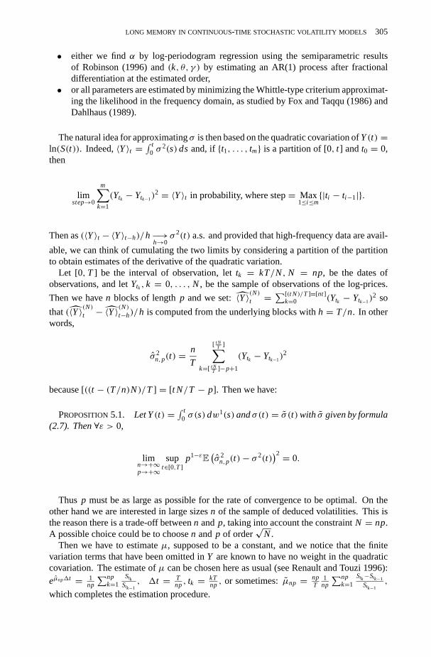
• either we findα by log-periodogram regression using the semiparametric resultsof Robinson (1996) and(k, θ, γ ) by estimating an AR(1) process after fractionaldifferentiation at the estimated order,

• or all parameters are estimated by minimizing the Whittle-type criterium approximat-ing the likelihood in the frequency domain, as studied by Fox and Taqqu (1986) andDahlhaus (1989).

The natural idea for approximatingσ is then based on the quadratic covariation ofY(t) =ln(S(t)). Indeed,〈Y〉t =

∫ t0 σ

2(s)ds and, if {t1, . . . , tm} is a partition of [0, t ] and t0 = 0,then

limstep→0

m∑k=1

(Ytk − Ytk−1)2 = 〈Y〉t in probability, where step= Max

1≤i≤m{|ti − ti−1|}.

Then as(〈Y〉t − 〈Y〉t−h)/h−→h→0

σ 2(t) a.s. and provided that high-frequency data are avail-

able, we can think of cumulating the two limits by considering a partition of the partitionto obtain estimates of the derivative of the quadratic variation.

Let [0, T ] be the interval of observation, lettk = kT/N, N = np, be the dates ofobservations, and letYtk , k = 0, . . . , N, be the sample of observations of the log-prices.

Then we haven blocks of lengthp and we set:〈Y〉(N)t = ∑[(t N)/T ]=[nt]k=0 (Ytk − Ytk−1)

2 so

that(〈Y〉(N)t − 〈Y〉(N)t−h)/h is computed from the underlying blocks withh = T/n. In other

words,

σ 2n,p(t) =

n

T

[ t NT ]∑

k=[ t NT ]−p+1

(Ytk − Ytk−1)2

because[((t − (T/n)N)/T ] = [t N/T − p]. Then we have:

PROPOSITION5.1. Let Y(t) = ∫ t0 σ(s)dw1(s) andσ(t) = σ (t)with σ given by formula

(2.7). Then∀ε > 0,

limn→+∞p→+∞

supt∈[0,T ]

p1−εE(σ 2

n,p(t)− σ 2(t))2 = 0.

Thus p must be as large as possible for the rate of convergence to be optimal. On theother hand we are interested in large sizesn of the sample of deduced volatilities. This isthe reason there is a trade-off betweenn andp, taking into account the constraintN = np.A possible choice could be to choosen and p of order

√N.

Then we have to estimateµ, supposed to be a constant, and we notice that the finitevariation terms that have been omitted inY are known to have no weight in the quadraticcovariation. The estimate ofµ can be chosen here as usual (see Renault and Touzi 1996):eµnp1t = 1

np

∑npk=1

StkStk−1

, 1t = Tnp, tk = kT

np , or sometimes:µnp = npT

1np

∑npk=1

Stk−Stk−1

Stk−1,

which completes the estimation procedure.


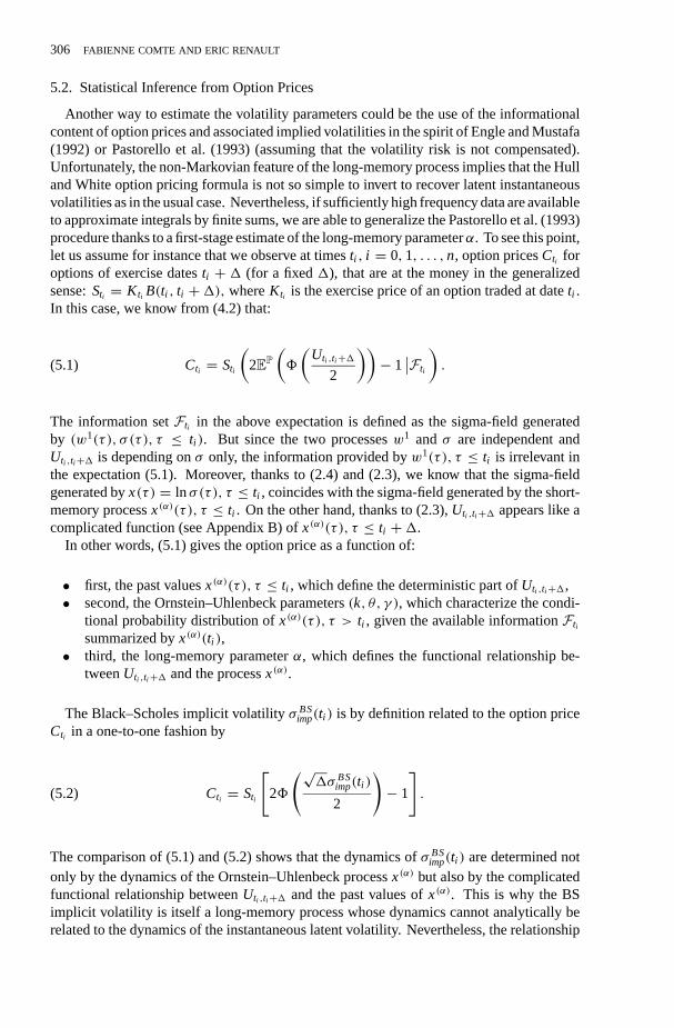
5.2. Statistical Inference from Option Prices

Another way to estimate the volatility parameters could be the use of the informationalcontent of option prices and associated implied volatilities in the spirit of Engle and Mustafa(1992) or Pastorello et al. (1993) (assuming that the volatility risk is not compensated).Unfortunately, the non-Markovian feature of the long-memory process implies that the Hulland White option pricing formula is not so simple to invert to recover latent instantaneousvolatilities as in the usual case. Nevertheless, if sufficiently high frequency data are availableto approximate integrals by finite sums, we are able to generalize the Pastorello et al. (1993)procedure thanks to a first-stage estimate of the long-memory parameterα. To see this point,let us assume for instance that we observe at timesti , i = 0,1, . . . ,n, option pricesCti foroptions of exercise datesti + 1 (for a fixed1), that are at the money in the generalizedsense:Sti = Kti B(ti , ti +1), whereKti is the exercise price of an option traded at dateti .In this case, we know from (4.2) that:

Cti = Sti

(2EP

(8

(Uti ,ti+1

2

))− 1

∣∣Fti

).(5.1)

The information setFti in the above expectation is defined as the sigma-field generatedby (w1(τ ), σ (τ ), τ ≤ ti ). But since the two processesw1 andσ are independent andUti ,ti+1 is depending onσ only, the information provided byw1(τ ), τ ≤ ti is irrelevant inthe expectation (5.1). Moreover, thanks to (2.4) and (2.3), we know that the sigma-fieldgenerated byx(τ ) = ln σ(τ), τ ≤ ti , coincides with the sigma-field generated by the short-memory processx(α)(τ ), τ ≤ ti . On the other hand, thanks to (2.3),Uti ,ti+1 appears like acomplicated function (see Appendix B) ofx(α)(τ ), τ ≤ ti +1.

In other words, (5.1) gives the option price as a function of:

• first, the past valuesx(α)(τ ), τ ≤ ti , which define the deterministic part ofUti ,ti+1,• second, the Ornstein–Uhlenbeck parameters(k, θ, γ ), which characterize the condi-

tional probability distribution ofx(α)(τ ), τ > ti , given the available informationFtisummarized byx(α)(ti ),

• third, the long-memory parameterα, which defines the functional relationship be-tweenUti ,ti+1 and the processx(α).

The Black–Scholes implicit volatilityσ BSimp(ti ) is by definition related to the option price

Cti in a one-to-one fashion by

Cti = Sti

[28

(√1σ BS

imp(ti )

2

)− 1

].(5.2)

The comparison of (5.1) and (5.2) shows that the dynamics ofσ BSimp(ti ) are determined not

only by the dynamics of the Ornstein–Uhlenbeck processx(α) but also by the complicatedfunctional relationship betweenUti ,ti+1 and the past values ofx(α). This is why the BSimplicit volatility is itself a long-memory process whose dynamics cannot analytically berelated to the dynamics of the instantaneous latent volatility. Nevertheless, the relationship


betweenUti ,ti+1 andx(α) can be approximated by (see Appendix B):

U2ti ,ti+1 =

∫ ti+1

ti

exp

(2∑τ<ti

(u− τ)α0(1+ α)1(x

(α)(τ ))

)× exp( f (x(α)(ti ); Z(u, ti , α))du,(5.3)

where f is a deterministic function andZ(u, ti , α) is a process independent ofFti .Thanks to Proposition 4.2, we can estimateα in a first step by a log-periodogram regres-

sion on the implicit volatilities. In a second stage, we shall assume thatα is known (the lackof accuracy due to estimatedα will not be considered here) and we propose the followingscheme for an indirect inference procedure, in the spirit of Pastorello et al. (1993):

θsimulation of−→ x(α)(t; θ) −→ Ct (θ)

BS−1+α-filter−→ (ln σ )(α)imp(θ) −→ β(θ)

CtBS−1+α-filter−→ (ln σ)(α)imp −→ β.

The meaning of this scheme is the following: for a given valueθ of the parameters of theOrnstein–Uhlenbeck processx(α), we are able to simulate a sample pathx(α)(t; θ); thenthanks to (5.3) and (5.1), we can get simulated valuesCt (θ) conformable to the Hull–Whitepricing. Of course, this procedure is computer intensive since the expectation (5.1) itself hasto be computed by Monte Carlo simulations. Nevertheless, as soon as option pricesCt (θ)

are available, the associated Black–Scholes implicit volatilitiesσimp(θ) are easy to compute,and finally, through the fractional differential operator, we obtain a process(ln σimp)

(α)(t; θ)whose dynamics should mimic the dynamics of the Ornstein–Uhlenbeck processx(α).

This proxy of the instantaneous volatility dynamics provides the basis of our indirectinference procedure. More precisely,β(θ) (respectively,β) denotes the pseudomaximumlikelihood estimator of the parameters of the simulated process(ln σimp)

(α)(t; θ) (respec-tively, the observed process(ln σimp)

(α)(t)) when the pseudolikelihood is defined by anOrnstein–Uhlenbeck modeling of these processes.

The basic idea of the indirect inference procedure is to compute a consistent estimatorof the structural parametersθ by solving inθ the equationsβ(θ) = β.

It is clear that the consistency proof of Gourieroux, Monfort, and Renault (1993) canbe easily extended to this setting thanks to the ergodicity property of the processes; on theother hand, the asymptotic probability distributions have to be reconsidered to take intoaccount the long-memory features.

6. SIMULATION AND EXPERIMENTS

6.1. Simulation of the Path of a Fractional Stochastic Volatility Price

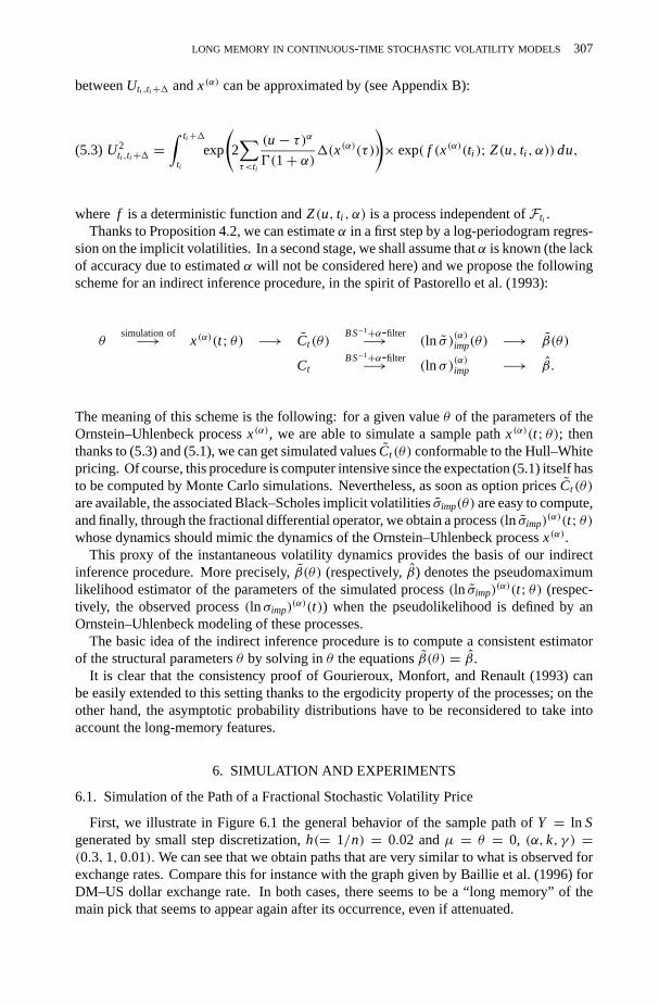
First, we illustrate in Figure 6.1 the general behavior of the sample path ofY = ln Sgenerated by small step discretization,h(= 1/n) = 0.02 andµ = θ = 0, (α, k, γ ) =(0.3,1,0.01).We can see that we obtain paths that are very similar to what is observed forexchange rates. Compare this for instance with the graph given by Baillie et al. (1996) forDM–US dollar exchange rate. In both cases, there seems to be a “long memory” of themain pick that seems to appear again after its occurrence, even if attenuated.


FIGURE6.1. Simulated path of log-stock price in the long-memory FSV model;N = 1000,h = 0.02,(α, k, γ ) = (0.3,1,0.01).

6.2. An Apparent Unit Root

Another comparison can be made with Baillie et al.’s (1996) work. Indeed, they arguethat their discrete time fractional model gives another representation of persistence that canremain stationary, contrary to usual unit roots models.

Here, we want to show that our model may exhibit an apparent unit root if a wrongparameterization is assumed for estimation. For that purpose, we look at what is obtainedif the model is estimated as if it were a GARCH(1,1) process:

{εt = ln St = σt zt , Et−1zt = 0,Vart−1zt = 1σ 2

t = ω + aε2t−1+ bσ 2

t−1.

In other words,(1− ϕL)ε2t = ω + (1− bL)νt whereϕ = a+ b andν is a white noise.

Weestimate theparameter(ω, ϕ,b) throughminimizingl (θ, ε1, . . . , εT ) =∑T

t=1(ln σ2t +

ε2t σ−2t ). The results are reported in Table 6.1 and Figure 6.2. One hundred forty samples

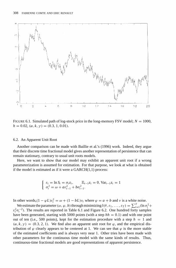
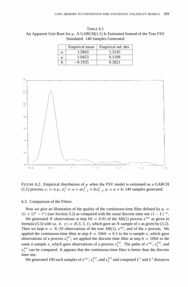
have been generated, starting with 5000 points (with a stephh = 0.1) and with one pointout of ten (i.e., 500 points), kept for the estimation procedure with a steph = 1 and(α, k, γ ) = (0.3,2,1). We find also an apparent unit root forϕ, and the empirical dis-tribution of ϕ clearly appears to be centered at 1. We can see thatϕ is the more stableof the estimated coefficients and is always very near 1. Other tries have been made withother parameters for the continuous time model with the same kinds of results. Thus,continuous-time fractional models are good representations of apparent persistence.


TABLE 6.1An Apparent Unit Root forϕ. A GARCH(1,1) Is Estimated Instead of the True FSV

Simulated. 140 Samples Generated

Empirical mean Empirical std. dev.ω 1.5843 1.3145ϕ 1.0453 0.1109b −0.1935 0.3821

FIGURE 6.2. Empirical distribution ofϕ when the FSV model is estimated as a GARCH(1,1) process;εt = σt zt , σ 2

t = ω + aε2t−1+ bω2

t−1, ϕ = a+ b; 140 samples generated.

6.3. Comparison of the Filters

Now we give an illustration of the quality of the continuous-time filter defined byai =((i + 1)α − i α) (see Section 3.2) as compared with the usual discrete time one(1− L)−α.

We generatedN observations at stephh = 0.01 of the AR(1) processx(α) as given informula (3.3) with(α, k, γ ) = (0.3,3,1), which gave anN-sample ofx as given by (3.2).Then we keptn = N/10 observations of the true AR(1),x(α), and of thex process. Weapplied the continuous-time filter at steph = 10hh = 0.1 to then-samplex, which gaveobservations of a processx(α)1 ; we applied the discrete time filter at steph = 10hh to thesamen-samplex, which gave observations of a processx(α)2 . The paths ofx(α), x(α)1 , andx(α)2 can be compared. It appears that the continuous-time filter is better than the discretetime one.

We generated 100 such samples ofx(α), x(α)1 , andx(α)2 and computedL1 andL2 distances


TABLE 6.2L1 andL2 Distances between the Original Paths and the Filtered Paths with the Two

Filters. Filter 1 Is the Continuous-Time Filter, Filter 2 the Discrete Time One

x(α), x(α)1 x(α), x(α)2dL1 0.1048 0.2135dL2 0.1359 0.3607

betweenx(α) andx(α)i , i = 1,2; that is,

dL1(x(α), x(α)i ) = 1

n

n∑j=1

|x(α)( j )− x(α)i ( j )|,

dL2(x(α), x(α)i ) = 1

n

n∑j=1

(x(α)( j )− x(α)i ( j ))2, i = 1,2.

The results are reported in Table 6.2. Even if the numbers do not have any meaning inthemselves, the comparison leads clearly to the conclusion that the first filter is significantlybetter. For a convincing comparison of the twelve first partial autocorrelations of the threesamples, see Comte (1996).

6.4. Estimation ofα by Log-Periodogram Regression in Three Models

Lastly, we compared the estimations ofα obtained by regression of lnI (λ) on lnλ, whereI (λ) is the periodogram (see Geweke and Porter-Hudak 1983 for the idea, Robinson 1996for the proof of the convergence and asymptotic normality of the estimator, and Comte 1996to check the assumptions given by Robinson).

We used 100 samples with length 400, where 4000 points were generated for thecontinuous-time models with a step 0.1 and one point out of ten was kept for the esti-mation. We had(α, k, γ ) = (0.3,3,1), in particularα = 0.3 in all cases.

But we compared two ways of estimatingα: either working directly on the log-period-ogram of the processx(t) = lnσ(t) (which exactly corresponds to our fractional Ornstein–Uhlenbeck model) or working onσ(t) = exp(x(t)), since it fulfills the same long-memoryproperties (see Proposition 2.2).

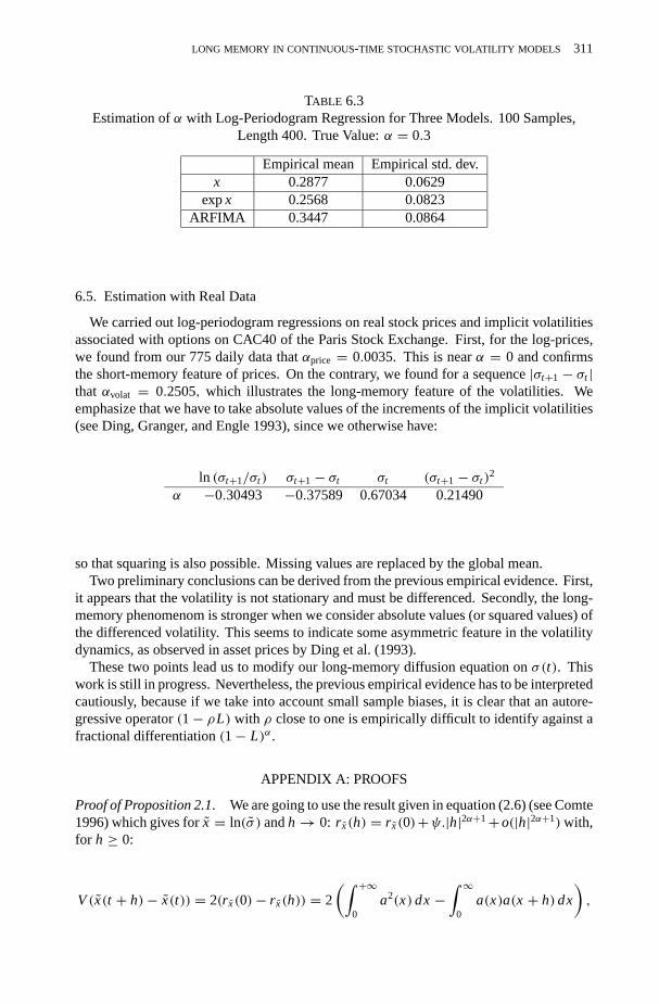
As a benchmark for this estimation ofα, we considered a third estimation through thefollowing procedure. Assuming that the observed path would be associated withx(t) =(1− L)−αx(α)(t) (with a sampling frequencyh = 1) instead ofx(t), we could then estimateα by a log-periodogram regression on the pathx(t), which is referred to below as theARFIMA method. The three methods should provide consistent estimators of the samevalue forα. The results are reported in Table 6.3: they are better withx than with anARFIMA model or with expx, and the recommendation is to work withx instead of expx.Let us nevertheless notice that the bad result for the ARFIMA model could be explained bythe fact that the discrete time filter(1− L)−α had been applied to the low frequency pathx(α)(t) with steph = 1.


TABLE 6.3Estimation ofα with Log-Periodogram Regression for Three Models. 100 Samples,

Length 400. True Value:α = 0.3

Empirical mean Empirical std. dev.x 0.2877 0.0629

expx 0.2568 0.0823ARFIMA 0.3447 0.0864

6.5. Estimation with Real Data

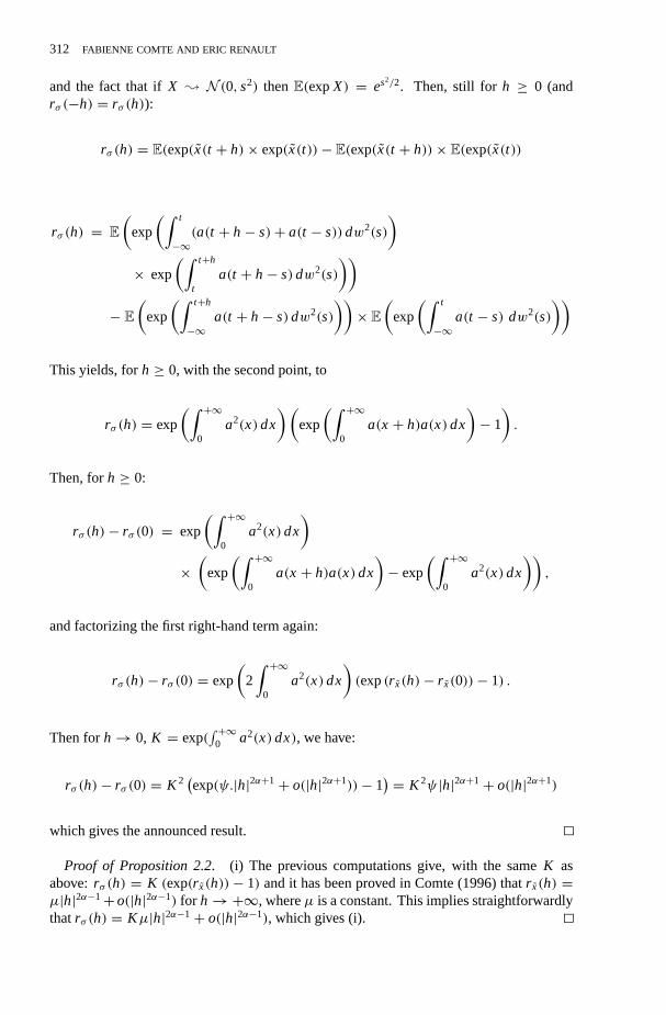
We carried out log-periodogram regressions on real stock prices and implicit volatilitiesassociated with options on CAC40 of the Paris Stock Exchange. First, for the log-prices,we found from our 775 daily data thatαprice = 0.0035. This is nearα = 0 and confirmsthe short-memory feature of prices. On the contrary, we found for a sequence|σt+1 − σt |that αvolat = 0.2505, which illustrates the long-memory feature of the volatilities. Weemphasize that we have to take absolute values of the increments of the implicit volatilities(see Ding, Granger, and Engle 1993), since we otherwise have:

ln (σt+1/σt ) σt+1− σt σt (σt+1− σt )2

α −0.30493 −0.37589 0.67034 0.21490

so that squaring is also possible. Missing values are replaced by the global mean.Two preliminary conclusions can be derived from the previous empirical evidence. First,

it appears that the volatility is not stationary and must be differenced. Secondly, the long-memory phenomenom is stronger when we consider absolute values (or squared values) ofthe differenced volatility. This seems to indicate some asymmetric feature in the volatilitydynamics, as observed in asset prices by Ding et al. (1993).

These two points lead us to modify our long-memory diffusion equation onσ(t). Thiswork is still in progress. Nevertheless, the previous empirical evidence has to be interpretedcautiously, because if we take into account small sample biases, it is clear that an autore-gressive operator(1− ρL) with ρ close to one is empirically difficult to identify against afractional differentiation(1− L)α.

APPENDIX A: PROOFS

Proof of Proposition 2.1. We are going to use the result given in equation (2.6) (see Comte1996) which gives forx = ln(σ ) andh→ 0: r x(h) = r x(0)+ψ.|h|2α+1+o(|h|2α+1)with,for h ≥ 0:

V(x(t + h)− x(t)) = 2(r x(0)− r x(h)) = 2

(∫ +∞0

a2(x)dx−∫ ∞

0a(x)a(x + h)dx

),


and the fact that ifX ; N (0, s2) thenE(expX) = es2/2. Then, still for h ≥ 0 (andrσ (−h) = rσ (h)):

rσ (h) = E(exp(x(t + h)× exp(x(t))− E(exp(x(t + h))× E(exp(x(t))

rσ (h) = E(

exp

(∫ t

−∞(a(t + h− s)+ a(t − s))dw2(s)

)× exp

(∫ t+h

ta(t + h− s)dw2(s)

))− E

(exp

(∫ t+h

−∞a(t + h− s)dw2(s)

))× E

(exp

(∫ t

−∞a(t − s) dw2(s)

))

This yields, forh ≥ 0, with the second point, to

rσ (h) = exp

(∫ +∞0

a2(x)dx

)(exp

(∫ +∞0

a(x + h)a(x)dx

)− 1

).

Then, forh ≥ 0:

rσ (h)− rσ (0) = exp

(∫ +∞0

a2(x)dx

)×(

exp

(∫ +∞0

a(x + h)a(x)dx

)− exp

(∫ +∞0

a2(x)dx

)),

and factorizing the first right-hand term again:

rσ (h)− rσ (0) = exp

(2∫ +∞

0a2(x)dx

)(exp(r x(h)− r x(0))− 1) .

Then forh→ 0, K = exp(∫ +∞

0 a2(x)dx), we have:

rσ (h)− rσ (0) = K 2(exp(ψ.|h|2α+1+ o(|h|2α+1))− 1

) = K 2ψ |h|2α+1+ o(|h|2α+1)

which gives the announced result.

Proof of Proposition 2.2. (i) The previous computations give, with the sameK asabove:rσ (h) = K (exp(r x(h))− 1) and it has been proved in Comte (1996) thatr x(h) =µ|h|2α−1+o(|h|2α−1) for h→+∞, whereµ is a constant. This implies straightforwardlythatrσ (h) = Kµ|h|2α−1+ o(|h|2α−1), which gives (i).


(ii)∫ +∞

0 rσ (h) cos(λh)dh = ∫ A0 rσ (h) cos(λh)dh + 1

λ

∫ +∞λA rσ (

uλ) cosudu. Now for

A chosen great enough, the development ofrσ near +∞ implies λ2α fσ (λ) =λ2α

∫ A0 rσ (h) cos(λh)dh+∫ +∞

λA u2α−1 cosudu+o(1),and consequently limλ→0 λ2α fσ (λ) =∫ +∞

0 u2α−1 cosuduwhere the integral is convergent near 0 because 2α > 0 and near+∞because:

∫ +∞1 u2α−1 cosudu= [u2α−1 sinu]+∞1 − (2α − 1)

∫ +∞1 u2α−2 sin uduwhere all

terms are obviously finite.

Proof of Lemma 3.1. For the proof of the first convergence:YnD⇒ Y on a compact set

[0, T ], we check theL2 pointwise convergence ofYn(t) towardY(t), and then a tightnesscriterion as given by Billingsley (1968, Th. 12.3):E|Yn(t2)− Yn(t1)|p ≤ C.|t2− t1|q withp > 0, q > 1, andC a constant.

TheL2 convergence is ensured by computing:

E(Yn(t)− Y(t))2 = E(∫ t

0

(σ

([ns]

n

)− σ(s)

)dw1(s)

)2

= E

(∫ t

0

(σ

([ns]

n

)− σ(s)

)2

ds

)

=∫ t

0E(σ

([ns]

n

)− σ(s)

)2

ds with Fubini.

Then theL2 convergence is obviously given by an inequality:E(σ (t2)− σ(t1))2 ≤ C.|t2−t1|γ for a positiveγ and a constantC.

As usual, letx(t) = ∫ t0 a(t − s)dw2(s) and lett1 ≤ t2.

E(σ (t2)− σ(t1))2 = E(exp(x((t2))− exp(x(t1)))2 = E (e2x(t2) + e2x(t1) − 2ex(t1)+x(t2)

)= e2

∫ t1

0a2(x)dx + e2

∫ t2

0a2(x)dx

− 2e12

∫ t1

0a2(x)dx+ 1

2

∫ t2

0a2(x)dx+

∫ t1

0a(x)a(t2−t1+x)dx

= e2∫ t2

0a2(x)dx

×(

1+ e−2∫ t2

t1a2(x)dx − 2e

− 32

∫ t2

t1a2(x)dx−

∫ t1

0a(x)(a(x)−a(t2−t1+x))dx

)≤ 2e2

∫ t2

0a2(x)dx

(1− e

− 32

∫ t2

t1a2(x)dx−

∫ t1

0a(x)(a(x)−a(t2−t1+x))dx

).

The term inside the last parentheses being necessarily nonnegative, the term in the lastgreat exponential is nonpositive. Moreover| ∫ t2

t1a2(x)dx| ≤ M2

1 |t2 − t1| with M1 =supx∈[0,T ] |a(x)|, and sincea is α-Holder,

∣∣∣∣∫ t1

0a(x)(a(x)− a(t2− t1+ x))dx

∣∣∣∣ ≤ Cα|t2− t1|α∫ t1

0|a(x)|dx ≤ Cα|t2− t1|αM1T,

which implies| ∫ t2t1

a2(x)dx+ ∫ t10 a(x)(a(x) − a(t2 − t1 + x))dx| ≤ M2|t2 − t1|α, with


M2 = M2(T). Then using that∀u ≤ 0, 0 ≤ 1− eu ≤ |u|, we haveE(σ (t2)− σ(t1))2 ≤2K 2M2|t2 − t1|α, α ∈ ]0, 1

2[ where K = exp(∫ +∞

0 a2(x)dx) as previously. Then,E(σ ([ns]/n)− σ(s))2 ≤ 2K 2M2(

1n )α gives:

E(Yn(t)− Y(t))2 ≤ 2K 2M2T

nα∀t ∈ [0, T ],

which ensures theL2 convergence.We use a straightforward version of Burkholder’s inequality (see Protter 1992, p. 174),

E|Mt |p ≤ CpE〈M〉p/2t , whereCp is a constant andMt a continuous local martingale,M0 = 0, to write (with an immediate adaptation of the proof on [t1, t2] instead of [0, t ]):

E|Yn(t2)− Yn(t1)|p = E∣∣∣∣∫ t2

t1

σ

([ns]

n

)dw1(s)

∣∣∣∣p ≤ CpE∣∣∣∣∫ t2

t1

σ 2

([ns]

n

)ds

∣∣∣∣p/2 .Let us choosep = 4:

E|Yn(t2)− Yn(t1)|4 ≤ C4E∣∣∣∣∫ t2

t1

σ 2

([ns]

n

)ds

∣∣∣∣2= C4

∫ ∫[t1,t2]2

E(σ 2

([nu]

n

)σ 2

([nv]

n

))du dv

≤ C4

∫ ∫[t1,t2]2

√Eσ 4× Eσ 4 du dv (σ given by (2.7))

= C4Eσ 4(t2− t1)2, Eσ 4 = exp

(8∫ +∞

0a2(x)ds

).

This gives the tightness and thus the convergence.The second convergence is deduced from the first one, the decomposition:Yn(t) =

Yn(t) + un(t), with un(t) = σ( [nt]n )(w

1(t) − w1( [nt]n )), and Theorem 4.1 of

Billingsley (1968): (XnD⇒ X andρ(Xn, Zn)

P−→ 0) ⇒ (ZnD⇒ X), whereρ(x, y) =

supt∈[0,T ] |x(t)−y(t)|.Hereρ(Yn, Yn) = sup|un(t)|andun(t) = M([nt]/n) is a martingaleso that Doob’s inequality (see Protter 1992, p. 12, Th. 20) gives:

E

(sup

t∈[0,T ]|un(t)|

)2

≤ 4 supt∈[0,T ]

E(un(t)2).

Then,

Eun(t)2 = E

(σ 2

([nt]

n

)(w1(t)− w1

([nt]

n

))2)

= E(σ 2

([nt]

n

))E(w1(t)− w1

([nt]

n

))2


=(

t − [nt]

n

)E(σ 2

([nt]

n

))≤ 1

nE(σ 2),

which achieves the proof.

Proof of Proposition 3.2.

• First we prove the following implication:

{YnD⇒ Y or tight

σnD⇒ σ or tight

and

(Yn(t)σn(t)

)L2−→

(Y(t)σ (t)

)imply

(Yn

σn

)D⇒(

Yσ

).

Indeed, the functional convergences of both sequences imply their tightness and thusthe tightness of the joint process. This can be seen from the very definition of tightnessas given in Billingsley (1968), that can be written forYn: ∀ε, ∃Kn (compact set) sothatP(Yn ∈ Kn) > 1− (ε/2) and then, for thisε, we have forσn: ∃K ′n (compact set)so thatP(σn ∈ K ′n) > 1− ε

2. Then:

P((Yn, σn) ∈ Kn × K ′n) = 1− P(Yn /∈ Kn or σn /∈ K ′n)

≥ 1− P(Yn /∈ Kn)− P(σn /∈ K ′n)

= P(Yn ∈ Kn)+ P(σn ∈ K ′n)− 1

≥ 1− ε.

Now, the tightness and the pointwiseL2 convergence of the couple imply the conver-gence of the joint process.

• Let us check the pointwiseL2 convergence ofYn:

E(Yn(t)− Y(t))2 = E

(∫ [nt]/n

0

(σn

([ns]

n

)− σ(s)

)dw1(s)+

∫ t

[nt]n

σ(s)dw1(s)

)2

=∫ [nt]/n

0E

((σn

([ns]

n

)− σ(s)

)2

ds +∫ t

[nt]/nE(σ 2(s)

)ds.

The last right-hand term is less than1nE(σ

2) and goes to zero whenn grows to infinityand the first right-hand term can be written, for the part under the integral, as

E(σn

([ns]

n

)− σ(s))2

)= E

(exp

(∫ [nt]/n

0a

(t − [ns]

n

)dw2(s)

)− exp

(∫ t

0a(t − s)dw2(s)

))2

.

Now, forXn andX followingN (0,EX2n)andN (0,EX2) respectively,E(eXn−eX)2 =


e2EX2n+e2EX2−2eE(Xn+X)2/2, which goes to zero whenn grows to infinity ifEX2

n −→n→+∞EX2 andE(Xn + X)2 −→

n→+∞4EX2.

This can be checked quite straightforwardly here withX = ∫ t0 a(t − s)dw2(s) and

Xn =∫ [nt]/n

0 a(t − [ns]n )dw2(s), so that:

EX2n =

∫ [nt]/n

0a2

(t − [ns]

n

)ds −→

n→+∞

∫ t

0a2(t − s)ds= EX2,

E(Xn + X)2 =∫ [nt]/n

0a2

(t − [ns]

n

)ds+

∫ t

0a2(t − s)ds

+ 2∫ [nt]/n

0a

(t − [ns]

n

)a(t − s)ds −→

n→+∞4EX2.

This result gives in fact bothL2 convergences ofYn(t) and ofσn(t).• The tightness ofσn is then known from Comte (1996) and the tightness ofYn can

be deduced from the proof of Lemma 3.1 withEσ 4n (t) instead ofEσ 4, which is still

bounded. 2

Proof of Proposition 4.1. We work with σ(t) = exp(∫ t−∞ a(t − s)dw2(s)), but the

results would obviously still be valid with the only asymptotically stationary version ofσ .We use here and for the proof of Proposition (4.2), the following result:

∀η ≥ 0, limh→+∞

h1−2α

(∫ +∞η

a(x)a(x + h)dx

)= C,(A.1)

whereC is a constant. This result can be straighforwardly deduced from Comte andRenault (1996) through rewriting the proof of the result about the long-memory propertyof the autocovariance function (extended here to the caseη 6= 0).

• We know thatyt = E(σ 2(t + 1) | Ft ) = exp(2∫ 1

0 a2(x)dx)exp(2∫ t−∞ a(t + 1−

s)dw2(s)). Then:

cov(yt+h, yt ) = E(yt+hyt )− E(yt+h)E(yt )

= exp

(4∫ 1

0a2(x)dx

)× E

(exp

(2∫ t+h

−∞a(t + h+ 1− s)dw2(s)

+ 2∫ t

−∞a(t + h− s)dw2(s)

))− exp

(4∫ 1

0a2(x)dx

)× exp

(4∫ +∞

0a2(x + 1)dx

)


= exp

(4∫ +∞

0a2(x)dx

)(exp

(4∫ +∞

1a(x + h)a(x)dx

)− 1

).

This proves the stationarity of they process, and, with (A.1), which gives the orderof the term inside the exponential, implies the announced orderh2α−1.

• E(σ (t + h) | Ft ), still with the stationary version ofσ , is given by

exp

(∫ t

−∞a(t + h− s)dw2(s)

)× exp

(1

2

∫ t+h

ta2(t + h− s)ds

).

Then, as(E(E(σ (t + h | Ft )))2 = (Eσ(t + h))2, we have:

Var(E(σ (t + h) | Ft )) = exp

(∫ h

0a2(x)dx

)× exp

(2∫ +∞

0a2(x + h)dx

)− exp

(∫ +∞0

a2(x)dx

)= exp

(∫ +∞0

a2(x)dx

)(exp

(∫ +∞h

a2(x)dx

)− 1

).

As a(x) = xαa(x) = xα−1.xa(x) = O(xα−1) for x → +∞ since we know thatlimx→+∞ xa(x) = a∞. Then, forh→+∞,

∫ +∞h

(xα−1)2(xa(x))2 dx = O

(a2∞

∫ +∞h

x2α−2 dx

)= O(h2α−1).

Developing again the exponential of this term for greath gives the orderh2α−1, andeven the limit of the variance divided byh2α−1 for h→+∞, which isK (a2

∞/1−2α)with K = exp(

∫ +∞0 a2(x)dx).

Forα = 0, a(x) = e−kx gives obviously for the variance an orderCe−kh.

Proof of Proposition 4.2. We have to compute cov(zt , zt+h).

E(zt+hzt ) = E(∫ 1

0E(σ 2(t + h+ u) | Ft+h)du×

∫ 1

0E(σ 2(t + v) | Ft )dv

)=∫ 1

0

∫ 1

0

[E(e(2∫ u

0a2(x)dx)e

(2∫ t+h

−∞ a(t+h+u−s)dw2(s))e(2∫ v

0a2(x)dx)e

(2∫ t

−∞ a(t+v−s)dw2(s)))]

du dv

=∫ 1

0

∫ 1

0

[e(2∫ u

0a2(x)dx+2

∫ v

0a2(x)dx)e

(2∫ t

−∞(a(t+h+u−s)+a(t+v−s))2 ds)e(2∫ t+h

ta2(t+h+u−s)ds)

]du dv

=∫ 1

0

∫ 1

0e(4∫ +∞

0a2(x)dx+4

∫ +∞0

a(x+h+u)a(x)dx) du dv.


Moreover, with thesamekindof computationswehaveE(zt+h)E(zt ) = exp(4∫ +∞

0 a2(x)dx)so that:

cov(zt , zt+h) = exp

(4∫ +∞

0a2(x)dx

)×[∫ 1

0

∫ 1

0

(exp

(4∫ +∞v

a(x + h+ u− v)a(x)dx

)− 1

)du dv

].

Thenz is stationary and another use of (A.1) gives the orderh2α−1 for h→+∞.

Proof of Proposition 4.3. Let Z(t) = ∫ t0 σ(u)dw

1(u). Then we know (see Protter 1992p. 174, for p = 4) thatEZ(t)4 = 4(4−1)

2 E∫ t

0 Z2(s)d〈Z〉s. As 〈Z〉s =∫ s

0 σ2(u)du, we

find: EZ(t)4 = 6E(∫ t

0 Z2(s)σ 2(s)ds) = 6∫ t

0 E(Z2(s)σ 2(s))ds, with Fubini’s theorem.

ThenE(Z2(t)σ 2(t)) = E(∫ t0 (σ (t)σ (u))dw1(u))2 = E ∫ t

0 (σ2(t)σ 2(u))du (σ andw1 are

independent). This yields

EZ(t)4 = 6∫ t

0

∫ s

0(rσ 2(|s− u|)+ (Eσ 2)2)du ds,

wherer is the autocovariance function, and, lastly,ϕ(h) = 3h2(Eσ 2)2 + 3∫∫

[0,h]2 rσ 2(|s−u|)du ds.

• Near zero, the autocovariance function ofσ 2 is of the same kind as the one ofσ , witha replaced by 2a, sinceσ = exp(x). Then we know from Proposition 2.1 that, forh→ 0: rσ 2(h) = rσ 2(0)+Ch2α+1+o(h2α+1),whereC is a constant andα ∈ ]0, 1

2[.Then replacing inϕ(h) gives

ϕ(h) = 3h2((Eσ 2)2+ rσ 2(0))+ 3C

(2α + 2)(2α + 3)h2α+3+ o(h2α+3).

For α = 0, a(x) = exp(−kx) givesrσ 2(h) = e2/k(exp( 2

k ekh)− 1)

which leads to:rσ 2(h) = rσ 2(0)− 2e4/kh+ o(h), for h→ 0. This implies the continuity forα = 0.Now,E(Y(h)− EY(h))2 = E(∫ h

0 σ(u)dw1(u))2 = E ∫ h0 σ

2(u)du= hEσ 2 impliesthat

limh→0

kurtY(h) = 3Eσ 4

(Eσ 2)2> 3.

• From Proposition 2.2, we know that, forα ∈ ]0, 12[ andh→+∞,

∫ ∫[0,h]2

rσ 2(|s− u|)du ds= O

(∫ ∫[1,h]2

u2α−1 du ds

)= O(h2α+1),

but for α = 0, rσ 2(h) = e2/k(

2k e−kh+ o(e−kh)

). This gives the result and the

exponential rate forα = 0. 2


Proof of Proposition 5.1. Let m= [Nt/T ], then

Eσ 2n,p(t) =

n

T

m∑k=m−p+1

E(∫ tk

tk−1

σ(s)dw1(s)

)2

= n

T

m∑k=m−p+1

E(∫ tk

tk−1

σ 2(s)ds

)

= n

TE

(∫ tm

tm−p

σ 2(s)ds

)= n

TE(σ 2)(tm − tm−p) = n

Tp× T

npEσ 2,= Eσ 2,

whereEσ 2 = exp( 12

∫ +∞0 a2(x)dx). This ensures theL1 convergence of the sequence,

uniformly in t .Before computing the mean square, let:

f (z) = f (|z|) = Eσ 2(u)σ 2(u+ |z|)= exp

(4∫ +∞

0a2(x)dx+ 4

∫ +∞0

a(x)a(x + |z|)dx

).

Then

E[σ 2n,p(t)− σ 2(t)]2 = E

[n

T

m∑k=m−p+1

(Ytk − Ytk−1)2− σ 2(t)

]2

= n2

T2E

[m∑

k=m−p+1

(Ytk − Ytk−1)2

]2

+ Eσ 4(t)− 2n

TE

[m∑

k=m−p+1

σ 2(t)(Ytk − Ytk−1)2

]2

.

We consider separately the different terms.

E[σ 2(t)(Ytk − Ytk−1)

2]2 = E

[∫ tk

tk−1

σ(t)σ (s)dw1(s)

]2

= E[∫ tk

tk−1

σ 2(t)σ 2(s)ds

]=∫ tk

tk−1

f (t − s)ds

asσ andw1 are independent. As in a previous proof, we have:

E[∫ tk

tk−1

σ(s)dw1(s)

]4

= 3∫ ∫

[tk−1,tk]2f (u− v)du dv,

and for j 6= k: E[(Ytk − Ytk−1)2(Ytj − Ytj−1)

2] = E(∫ tktk−1σ 2(s)ds× ∫ tj

tj−1σ 2(s)ds). This


gives:

E

[m∑

k=m−p+1

(Ytk − Ytk−1)2

]2

= 2m∑

k=m−p+1

∫ ∫[tk−1,tk]2

f (u− v)du dv

+∫ ∫

[tm−p,tm]2f (u− v)du dv.

Now with all the terms:

E[σ 2n,p(t)− σ 2(t)] = n2

T2

(2

m∑k=m−p+1

∫ ∫[tk−1,tk]2

f (u− v)du dv

+∫ ∫

[tm−p,tm]2f (u− v)du dv

)

+ Eσ 4(t)− 2n

T

∫[tm−p,tm]

f (t − s)ds

= 2n2

T2

m∑k=m−p+1

∫ ∫[tk−1,tk]2

( f (u− v)− f (0))du dv

+ n2

T2

∫ ∫[tm−p,tm]2

( f (u− v)− f (0))du dv

− 2n

T

∫[tm−p,tm]

( f (t − s)− f (0))ds+ 2Eσ 4

p.

Let K1 = exp(8∫ +∞

0 a2(s)ds). Then f (h) = K1rσ (h) whererσ is as in Proposition 2.1.Proposition 2.1 then implies| f (h) − f (0) |≤ K1C | h |2α+1, whereC is a positiveconstant.

This implies that:∀ε > 0, ∃η > 0, so that|v − u| < η⇒ | f (v − u)− f (0)| < ε. Letthenε = 1/p, thenη = η(ε) is fixed and

E[σ 2n,p(t)−σ 2(t)]2 ≤ 2n2

T2× p×

(T

np

)2

× 1

p+ n2

T2×(

T

n

)2

× 1

p+ 2n

T× p

T

np× 1

p+2Eσ 2

p

if |tm − tm−p| = Tn < η, which implies|tk − tk−1| = T

np < η. Then

E[σ 2n,p(t)− σ 2(t)]2 ≤

(2

p+ 1+ 2+ 2Eσ 2

)× 1

p=(

2

p+ 3+ 2Eσ 2

)× 1

p.

Then∀a > 0, n > T/η⇒ p1−a.E[σ 2

n,p(t)− σ 2(t)]2 ≤ C

pa, whereC = 5+ 2Eσ 2.

Thestationarity implies that the result isuniform int , so that limn,p−→+∞ sup

t∈[0,T ]p1−aE[σ 2

n,p(t)

− σ 2(t)]2 = 0.


APPENDIX B

We suppose herer = 0 andλ2 = 0, so thatx(α)(t) = (ln σ)(α)(t) can be written:

x(α)(t) = e−kt

(x(α)(0)+

∫ t

0eksγ dw2(s)

).

ThenU2t,T =

∫ Tt σ

2(u)du can be written:

U2t,T =

∫ T

texp

(2∫ t

0

(u− s)α

0(1+ α) dx(α)(s)

)× exp

(2∫ u

t

(u− s)α

0(1+ α) dx(α)(s)

)du.

Then the first part, exp(2∫ t

0(u−s)α

0(1+α) dx(α)(s)), is “deterministic” knowingFt . For the second

part, since we have fors > t thatx(α)(s) = e−k(s−t)xα(t)+ ∫ st e−k(s−x)γ dw2(x), we find

that

x(α)(s) = e−k(t−s)x(α)(t)+∫ t

sek(s−x)γ dw2(x),

∫ u

t

(u− s)α

0(1+ α) dx(α)(s) = x(α)(t)×(−k

∫ u

t

(u− s)α

0(1+ α)e−k(s−t) ds

)− k

∫ u

t

(u− s)α

0(1+ α)∫ s

tek(s−x)γ dw2(x)

+γ∫ u

t

(u− s)α

0(1+ α) dw2(s).

This term depends then only on(x(α)(t)) and onfuture increments of the Brownianmotionw2; those increments are independent ofFt . This is the reason we can write

exp

(2∫ u

t

(u− s)α

0(1+ α) dx(α)(s)

)= f (x(α)(t); Z(u, t, α)).

At time t = ti , this gives the announced formula, with ln[f (x(α)(t); Z(u, t, α))] =x(α)(t)ϕ(t,u)+ Z(u, t, α); ϕ(t,u) is a deterministic function,Z(u, t, α) is a process inde-pendent ofFt :

Z(t,u, α) = −k∫ u

t

(u− s)α

0(1+ α)∫ s

tek(s−x)γ dw2(x)+ γ

∫ u

t

(u− s)α

0(1+ α) dw2(s).

REFERENCES

BACKUS, D. K. and S. E. ZIN (1993): Long-Memory Inflation Uncertainty: Evidence from the TermStructure of Interest RatesJ. Money, Credit, Banking3, 681–700.


BAILLIE , R. T., T. BOLLERSLEV, and H. O. MIKKELSEN (1996): Fractionally Integrated GeneralizedAutoregressive Conditional Heteroskedasticity,J. Econometrics74, 1, 3–30.

BILLINGSLEY, P. (1968):Convergence of Probability Measures. New York: Wiley.

BLACK, F. and M. SCHOLES (1973): The Pricing of Options and Corporate Liabilities,J. PoliticalEcon.3, 637–654.

BREIDT, F. J., N. CRATO, and P. DE LIMA (1993): Modeling Long-Memory Stochastic Volatility,discussion paper, Iowa State University.

COMTE, F. (1996): Simulation and Estimation of Long Memory Continuous Time Models,J. TimeSeries Anal.17, 1, 19–36.

COMTE, F. and E. RENAULT (1996): Long Memory Continuous Time Models,J. Econometrics73,101–149.

DALHUAS, R. (1989): Efficient Parameter Estimation for Self-Similar Processes,Ann. Statistics17,4, 1749–1766.

DELBAEN, F. and W. SCHACHERMAYER (1994): A General Version of the Fundamental Theorem ofAsset Pricing,Math. Ann.300, 3, 463–520.

DING, Z., C., W. J. GRANGER, and R. F. ENGLE (1993): A Long Memory Property of Stock MarketReturns and a New Model,J. Empirical Finance1, 1.

DROST, F. C. and B. J. M. WERKER (1996): Closing the GARCH Gap: Continuous Time GARCHModeling,J. Econometrics74, 31–58.

ENGLE, R. F. and C. MUSTAFA (1992): Implied ARCH Models from Options Prices,J. Econometrics52, 289–331.

FOX, R. and M. S. TAQQU (1986): Large Sample Properties of Parameter Estimates for StronglyDependent Time Series,Ann. Statistics14, 517–532.

GEWEKE, J. and S. PORTER-HUDAK (1983): The Estimation and Application of Long Memory TimeSeries Models,J. Time Series Analysis4, 221–238.

GHYSELS, E., A. HARVEY, and E. RENAULT (1996): Stochastic Volatility; InHandbook of Statistics,Vol. 14, Statistical Methods in Finance, G. S. Maddala, ed. Amsterdam: North Holland, Ch. 5,119–191.

GOURIEROUX, C., A. MONFORT, and E. RENAULT (1993): Indirect Inference,J. Appl. Econometrics8, S85–S118.

HARRISON, J. M. and D. M. KREPS(1981): Martingale and Arbitrage in Multiperiods SecuritiesMarkets,J. Econ. Theory20, 381–408.

HARVEY, A. C. (1993): Long Memory in Stochastic Volatility, London School of Economics, workingpaper.

HARVEY, A., E. RUIZ, and N. SHEPHARD(1994): Multivariate Stochastic Variance Models,Rev. Econ.Stud.61, 2, 247–264.

HEYNEN, R., A. KEMNA, and T. VORST(1994): Analysis of the Term Structure of Implied Volatilities,J. Financial Quant. Anal.29, 31–56.

HULL, J. and A. WHITE (1987): The Pricing of Options on Assets with Stochastic Volatilities,J.Finance3, 281–300.

JACQUIER, E., N. G. POLSON, and P. E. ROSSI (1994): Bayesian Analysis of Stochastic VolatilityModels (with discussion),J. Bus. & Econ. Statistics12, 371–417.

KARATZAS, I. and S. E. SHREVE (1991).Brownian Motion and Stochastic Calculus, 2nd ed. NewYork: Springer-Verlag.

MANDELBROT, B. B. and VAN NESS(1968): Fractional Brownian Motions, Fractional Noises andApplications,SIAM Rev.10, 422–437.

MELINO, A. and TURNBULL, S. M. (1990): Pricing Foreign Currency Options with Stochastic Volatil-ity, J. Econometrics45, 239–265.

MERTON, R. (1973): The Theory of Rational Option Pricing,Bell J. Econ. Mgmt. Sci.4, 141–183.


NELSON, D. B. and D. P. FOSTER(1994): Asymptotic Filtering Theory for ARCH Models,Econo-metrica1, 1–41.

PASTORELLO, S., E. RENAULT, and N. TOUZI (1993): Statistical Inference for Random VarianceOption Pricing,Southern European Economics Discussion Series.

PHAM, H. and N. TOUZI (1996): Intertemporal Equilibrium Risk Premia in a Stochastic VolatilityModel,Math. Finance6, 215–236.

PROTTER, P. (1992):Stochastic Integration and Differential Equations. New York: Springer-Verlag.

RENAULT, E. and N. TOUZI (1996): Option Hedging and Implicit Volatilities in a Stochastic VolatilityModel,Math. Finance6, 279–302.

ROBINSON, P. M. (1993): Efficient Tests for Nonstationary Hypotheses, Working paper, LondonSchool of Economics.

ROBINSON, P. M. (1996): Semiparametric Analysis of Long-Memory Time Series,Ann. Statistics22,515–539.

ROGERS, L. C. G. (1995): Arbitrage with Fractional Brownian Motion, University of Bath, discussionpaper.

ROZANOV, YU. A. (1968):Stationary Random Processes. San Francisco: Holden-Day.

SCOTT, L. (1987): Option Pricing when the Variance Changes Randomly: Estimation and an Appli-cation,J. Financial and Quant. Anal.22, 419–438.

Documents

LONG MEMORY IN CONTINUOUS-TIME STOCHASTIC … · Mathematical Finance, Vol. 8, No. 4 (October 1998), 291–323 LONG MEMORY IN CONTINUOUS-TIME STOCHASTIC VOLATILITY MODELS FABIENNE