Long-Duration Proximity Operations Flexibly

Optimized for Efficient Inspection and Servicing

Using Free-Orbit Dynamics

by

Zachary K. Funke

B.S., United States Air Force Academy (2015)

Submitted to the Department of Aeronautics and Astronauticsin partial fulfillment of the requirements for the degree of

Master of Science in Aeronautics and Astronautics

at the

MASSACHUSETTS INSTITUTE OF TECHNOLOGY

June 2017

c Massachusetts Institute of Technology 2017. All rights reserved.

Author . . . . . . . . . . . . . . . . . . . . . . . . . . . . . . . . . . . . . . . . . . . . . . . . . . . . . . . . . . . . . .Department of Aeronautics and Astronautics

May 25, 2017

Certified by. . . . . . . . . . . . . . . . . . . . . . . . . . . . . . . . . . . . . . . . . . . . . . . . . . . . . . . . . .Alvar Saenz-Otero

Principal Research Scientist, Aeronautics and AstronauticsDirector, MIT Space Systems Laboratory

Thesis Supervisor

Certified by. . . . . . . . . . . . . . . . . . . . . . . . . . . . . . . . . . . . . . . . . . . . . . . . . . . . . . . . . .David W. Miller

Professor of Aeronautics and AstronauticsThesis Supervisor

Accepted by . . . . . . . . . . . . . . . . . . . . . . . . . . . . . . . . . . . . . . . . . . . . . . . . . . . . . . . . .Youssef M. Marzouk

Associate Professor of Aeronautics and AstronauticsChair, Graduate Program Committee

2

Long-Duration Proximity Operations Flexibly Optimized for

Efficient Inspection and Servicing Using Free-Orbit Dynamics

byZachary K. Funke

Submitted to the Department of Aeronautics and Astronauticson May 25, 2017, in partial fulfillment of the

requirements for the degree ofMaster of Science in Aeronautics and Astronautics

Abstract

Satellites at geosynchronous orbital altitudes are highly valuable for national de-fense, but are also difficult to access and monitor. Uncrewed inspection spacecraftcould supervise various essential defense platforms and deter covert rendezvous byadversaries with malicious intent. ‘Neighborhood watch’ satellites tasked with this sit-uational awareness mission should be designed and operated in such a way as to max-imize their lifespan and efficacy. Motivated by this requirement, this thesis exploresthe prolonged medium- to close-range spacecraft proximity operations problem fromthe perspective of continuous optimal trajectory control. A numerical optimizationframework is presented for developing and analyzing fuel-, energy-, and time-optimaltrajectories with multiple phases using Gauss pseudospectral collocation software. Em-phasis is placed on energy efficiency during inspection, for which accurate dynamicalmodels play a critical role in formationkeeping fuel consumption. Various scenariosare analyzed for minimum-energy solutions, such as tactical phasing and insertion intoperiodic trajectories, avoidance of ‘no-fly’ zones, inclusion of coupling attitude dy-namics, and operations with highly-eccentric targets. This thesis focuses primarily onproximity operations carried out in geosynchronous orbital regimes and neglects orbitperturbations, instead determining the pure cost of linearizing Keplerian gravity usingthe Hill-Clohessy-Wiltshire model. Error in relative position, angular rate of circum-navigation, and fuel use to enforce linearized periodic trajectories are characterized. Itwas determined that proximity operations utilizing low-thrust high-specific-impulse so-lar electric propulsion are well-suited to minimum-energy trajectory optimization withthis method. While the contributed analysis tool is not suitable for on-board optimaltrajectory generation, it provides a framework to perform useful pre-mission analyses.

Thesis Supervisor: Dr. Alvar Saenz-OteroDirector, Space Systems Laboratory

Thesis Supervisor: Dr. David W. MillerProfessor of Aeronautics and Astronautics

3

4

Acknowledgements

This work was funded entirely by the USAF Space Command Fellowship. Anystatements made in this thesis do not reflect the official views of the Department ofDefense, United States Air Force, MIT, or any of their affiliated organizations.

I would like to thank the following people for their friendship and guidance:

• My loving wife, Katy, for her uncompromising support, proofreading, and pa-tience. Without her, this thesis wouldn’t exist.

• My entire family for all of their encouragement, especially my Mom for makingme laugh and teaching me attention to detail, and my Dad for teaching me mathand how to think critically.

• The SPHERES team of the Space Systems Lab, especially:

William Sanchez for his grounded, methodical, and persevering approach toaccomplishing the research objectives of the lab,

Antonio Teran Espinoza for his wellspring of optimism and ingenious problem-solving ability,

Chris Jewison, David Sternberg, Tim Setterfield, and Max Yates for theirexperienced mentorship in the realms of satellite engineering, control systemsengineering, and the analysis of proximity operations,

and Dr. Danilo Roascio, whose superhuman focus and work ethic is paralleledonly by his skill as an electrical and computer engineer.

• Dr. Alvar Saenz-Otero, my official thesis advisor, and Professor David Miller fortheir invaluable guidance over my graduate education.

• An extra special thanks to Patrick O’Shea for picking up his phone and callingme at 8:57 a.m. on Monday, December 19th, 2016 to inform me of our final examstarting at 9:00 a.m. that morning.

5

6

Table of Contents

1 Introduction 131.1 Motivation . . . . . . . . . . . . . . . . . . . . . . . . . . . . . . . . . 131.2 Objective . . . . . . . . . . . . . . . . . . . . . . . . . . . . . . . . . 151.3 Outline of Thesis . . . . . . . . . . . . . . . . . . . . . . . . . . . . . 161.4 Literature Review . . . . . . . . . . . . . . . . . . . . . . . . . . . . . 18

1.4.1 Approach to Literature Review . . . . . . . . . . . . . . . . . 181.4.2 Acceleration Models for Relative Motion . . . . . . . . . . . . 181.4.3 Proximity Operations with Free-Orbit Trajectories . . . . . . 211.4.4 Continuous-Thrust Trajectory Optimization for Proximity Op-

erations . . . . . . . . . . . . . . . . . . . . . . . . . . . . . . 271.4.5 Summary of Review . . . . . . . . . . . . . . . . . . . . . . . 31

2 Long-Duration Satellite Proximity Operations 332.1 Relative Orbital Dynamics . . . . . . . . . . . . . . . . . . . . . . . . 34

2.1.1 The LVLH Coordinate Frame . . . . . . . . . . . . . . . . . . 352.1.2 The Full Keplerian Nonlinear Equations of Relative Motion . . 352.1.3 The Hill-Clohessy-Wiltshire Model . . . . . . . . . . . . . . . 38

2.2 Comparison of Classes of Nonlinear and Linearized Relative MotionTrajectories . . . . . . . . . . . . . . . . . . . . . . . . . . . . . . . . 43

2.3 Constraint Specification for Design of Periodic Relative Trajectories . 542.3.1 Specifying the Clohessy-Wiltshire Free-Orbit Ellipse . . . . . . 562.3.2 Specifying Keplerian Relative Periodic Trajectories . . . . . . 61

2.4 Angular Rate of Circumnavigation . . . . . . . . . . . . . . . . . . . 732.4.1 Periodic Trajectory Linearization Error for a Near-Circular Ref-

erence Orbit . . . . . . . . . . . . . . . . . . . . . . . . . . . . 742.5 Effects of Orbit Perturbations on Relative Dynamics . . . . . . . . . 782.6 Chapter Summary . . . . . . . . . . . . . . . . . . . . . . . . . . . . 81

3 Optimal Control Problem Formulation 833.1 The Optimal Control Problem . . . . . . . . . . . . . . . . . . . . . . 84

3.1.1 The 3-DOF Formulation . . . . . . . . . . . . . . . . . . . . . 843.1.1.1 The Minimum-Energy Problem . . . . . . . . . . . . 87

7

3.1.1.2 The Minimum-Fuel Problem . . . . . . . . . . . . . . 893.1.1.3 The Minimum-Time Problem . . . . . . . . . . . . . 91

3.1.2 Determining the Existence of Singular Arcs in the Solution . . 923.1.3 Including Attitude Dynamics: The 6-DOF Formulation . . . . 95

3.2 Insights Gained from Preliminary Analysis . . . . . . . . . . . . . . . 993.2.1 Over-Actuation in the Problem Formulation . . . . . . . . . . 993.2.2 When is Attitude Coupling Required? . . . . . . . . . . . . . 99

3.3 Numerical Optimization with GPOPS-II . . . . . . . . . . . . . . . . 1033.3.1 Numerical Optimization Method . . . . . . . . . . . . . . . . 1043.3.2 Implementation Approach . . . . . . . . . . . . . . . . . . . . 106

3.3.2.1 Instantiation Shell . . . . . . . . . . . . . . . . . . . 1083.3.2.2 Main . . . . . . . . . . . . . . . . . . . . . . . . . . . 1093.3.2.3 Continuous . . . . . . . . . . . . . . . . . . . . . . . 1103.3.2.4 Endpoint . . . . . . . . . . . . . . . . . . . . . . . . 110

3.4 Chapter Summary . . . . . . . . . . . . . . . . . . . . . . . . . . . . 112

4 Results 1154.1 Approach to Results Chapter . . . . . . . . . . . . . . . . . . . . . . 1164.2 Validation and Preliminary Results . . . . . . . . . . . . . . . . . . . 117

4.2.1 Linear Quadratic Regulator . . . . . . . . . . . . . . . . . . . 1184.2.2 Minimum-Fuel Rendezvous . . . . . . . . . . . . . . . . . . . . 1194.2.3 Minimum-Energy Rendezvous . . . . . . . . . . . . . . . . . . 1234.2.4 Minimum-Time Rendezvous . . . . . . . . . . . . . . . . . . . 125

4.2.4.1 Scheduling Policy . . . . . . . . . . . . . . . . . . . . 1274.2.4.2 Time-Energy Hybrid . . . . . . . . . . . . . . . . . . 1284.2.4.3 Including Coupling Attitude Dynamics . . . . . . . . 129

4.2.5 Summary of Preliminary Results . . . . . . . . . . . . . . . . 1314.3 Demonstration of Path Constraints, Phasing, and Nonlinear Dynamics 133

4.3.1 No-Fly Zone Avoidance . . . . . . . . . . . . . . . . . . . . . 1334.3.2 Optimal Period Matching . . . . . . . . . . . . . . . . . . . . 1354.3.3 Highly-Eccentric Rendezvous . . . . . . . . . . . . . . . . . . 1364.3.4 Summary of Intermediate Results . . . . . . . . . . . . . . . . 140

4.4 Long-Duration Proximity Operations . . . . . . . . . . . . . . . . . . 1404.4.1 Free-Orbit Trajectory Design . . . . . . . . . . . . . . . . . . 141

4.4.1.1 Clohessy-Wiltshire Relative Dynamics . . . . . . . . 1414.4.1.2 Keplerian Relative Dynamics . . . . . . . . . . . . . 148

4.4.2 Cost of Linearization Revisited . . . . . . . . . . . . . . . . . 1514.5 Summary of Results . . . . . . . . . . . . . . . . . . . . . . . . . . . 158

5 Conclusions 1615.1 Thesis Summary . . . . . . . . . . . . . . . . . . . . . . . . . . . . . 1615.2 List of Contributions . . . . . . . . . . . . . . . . . . . . . . . . . . . 163

8

5.3 Conclusions . . . . . . . . . . . . . . . . . . . . . . . . . . . . . . . . 1645.4 Future Work . . . . . . . . . . . . . . . . . . . . . . . . . . . . . . . . 165

5.4.1 Improvements to R/POTATO . . . . . . . . . . . . . . . . . . 1655.4.2 Graphical Model Approach for On-Orbit State Estimation . . 167

A Keplerian Orbital Mechanics 171A.1 The Classical Orbital Elements . . . . . . . . . . . . . . . . . . . . . 174A.2 Describing Angular Motion . . . . . . . . . . . . . . . . . . . . . . . . 178A.3 Orbital Perturbations . . . . . . . . . . . . . . . . . . . . . . . . . . . 180

B Nonlinear Solver Error Analysis 183

C Quaternion Convention 191C.1 Quaternion Convention for R/POTATO . . . . . . . . . . . . . . . . 191C.2 Partial Results from Minimum-Time Period Matching . . . . . . . . . 198

D List of R/POTATO User-Specifiable Parameters 205

9

10

Nomenclature

∆V Change in velocity

J2 Second zonal harmonic (oblate-Earth effect)

(H)CW (Hill-)Clohessy-Wiltshire

3-DOF 3-Degrees-of-Freedom

6-DOF 6-Degrees-of-Freedom

COE Classical (Keplerian) Orbital Element

DCM Direction Cosine Matrix

GEO Geosynchronous orbital regime

GPOPS-II Gauss Pseudospectral Optimization Software (Patterson and Rao [30])

GPS Global Positioning System

ISS International Space Station

LEO Low Earth Orbit

LQR Linear Quadratic Regulator

LTI Linear and Time-Invariant

LVLH Local Vertical, Local Horizontal

MEO Medium Earth Orbit

MIMO Multi-Input, Multi-Output

NFU Normalized Fuel Units (total impulse divided by maximum thrust)

NLEM Nonlinear Equation of Motion

PCO Projected Circular Orbit

11

PMP Pontryagin’s Minimum Principle

R/POTATO Rendezvous / Proximity Operations Trajectory Analysis Tool

RPO Rendezvous and Proximity Operations

RSO Resident Space Object

SISO Single-Input, Single-Output

SLAM Simultaneous Localization and Mapping

STK Systems Tool Kit (AGI [36])

TPBVP Two-Point Boundary Value Problem

TS Tschauner-Hempel

12

Chapter 1

Introduction

1.1 Motivation

It is often said that space is the ultimate high ground. From intelligence gathered

by surveillance platforms in low Earth orbit, to weather sensing and prediction data,

to scientific research carried out by space-based telescopes, to terrestrial navigation

capabilities provided by GPS, the information that is obtained from satellites is in-

dispensable for national defense and has become a vital element of societal function.

However, the orbital environment is characterized by many factors which make the

use of satellites inherently difficult.

For one, it is expensive and time-consuming to build, test, and launch a satellite

into its mission orbit, as well as moderately risky (although half a century of effort on

the part of spacelift organizations have greatly helped in this last regard). Secondly,

it is at least as expensive to repair or service satellites already in orbit, and technically

challenging to do so; for this reason, on-orbit servicing has been exceedingly rare and

reserved for only the most valuable of national assets, such as the 1993 servicing of

the Hubble Space Telescope.

Thirdly, and of increasing concern for national defense strategy, is the inherent

vulnerability of space-based assets. Outside of radio-frequency ground tracking and

13

mathematical modeling, the ability to determine the whereabouts and activities of

all satellites is limited; the use of optical telescopes to directly sense objects in orbit

is restricted by the geographical location of these facilities and the weather over-

head. Whereas launches of kinetic anti-satellite ballistic missiles can be relatively

easily detected (this capability being incidentally greatly augmented by space-based

surveillance platforms), covert rendezvous operations by a rogue spacecraft could

quickly and stealthily degrade or destroy an asset. A concerted combination of acts

such as these could blind or cripple a significant portion of space-based platforms and

the services they provide to American citizens and the nation’s defense, as well as

the defense of its allies. If national defense operations could not operate effectively

in such an intelligence-degraded environment, the urgent restoration of these assets

would undoubtedly need to occur at great cost. All the while, escalation of adversarial

activities in space could litter strategically-valuable orbital regimes with debris and

unresponsive satellites. This scenario could eventually lead to a ‘Kessler Syndrome’

outcome, tragically denying all people the continued peaceful use of space. It is thus

in the best interest of all users that a robust ‘neighborhood watch’ of difficult-to-

monitor regimes, such as the GEO belt, be implemented to deter potential covert

military acts and to increase the general level of transparency.

Additionally, in order to alleviate the challenges and costs associated with satellite

operations, the ability to cheaply service and repair satellites is of great interest to

the U.S. military, space agencies, and private corporations alike. A vital capability of

on-orbit inspectors and servicers is the ability to loiter at a safe distance from objects

of interest in order to gather information about them and plan the next stages of

the proximity operations. Being able to perform this in a fuel-efficient manner would

extend the useful mission life of these inspection and servicing satellites.

It is thought that solar electric propulsion will greatly increase the fuel efficiency

14

of spacecraft. These devices use magnetic or electrostatic fields to accelerate small

amounts of propellant to exhaust velocities in the tens of kilometers per second,

resulting in a very high ratio of force per unit propellant mass (specific impulse)

relative to that of conventional chemical monopropellant space propulsion. Operating

within the practical limits of spacecraft power subsystems, these devices produce low

thrust (on the scale of micronewtons to tens of millinewtons) with a very low rate of

propellant expenditure. They can be throttled over a range of forces by modifying

the strength of the accelerating field.

The fuel efficiency made possible by electric propulsion could be beneficial for long-

duration proximity operations by medium-sized robotic spacecraft. To take fullest

advantage of this technology, principles of optimal control should leverage natural

relative orbital dynamics to minimize or avoid fuel use along trajectories while ac-

complishing mission objectives.

1.2 Objective

The objective of this thesis is to provide a framework for analyzing optimal prox-

imity operations trajectories that can extend the mission life of on-orbit inspection

and servicing spacecraft. This should be done with a technique that is well-suited

to optimizing continuous-control problems, allows realistic modeling of the satellite’s

physical properties and constraints, and is flexible enough to accommodate a variety

of goals that may be relevant to a proximity operations mission. This tool should

allow for many different analyses to be obtained pertaining to the optimal trajectory

solution; for example, the ability to quantify the cost of linearizing orbital dynamics

under a variety of circumstances. Most importantly, the framework should allow for

the analysis of trajectories that incorporate free-orbit (thrust-less) trajectories in the

15

relative space around the object of interest with sizes, locations, and orientations that

can be designed by the user. This thesis should adequately motivate the need for this

numerical optimization technique by exploring the shortcomings of linearized equa-

tions of motion, as well as the circumstances under which more complicated dynamics

are necessitated for physical consistency. It should also validate the solutions provided

by the framework and demonstrate the problem-solving process with representative

analyses.

1.3 Outline of Thesis

1. Introduction. The thesis is motivated, the thesis objective is provided, and a

review of the relevant literature is conducted.

2. Long-Duration Satellite Proximity Operations. Relative Keplerian or-

bital dynamics are developed in full nonlinear form, followed by the common

linearized form. Classes of periodic trajectories are visualized and compared

under both models, and the cost of linearization is explored. Techniques for

specifying the size, shape, and orientation of periodic trajectories are proposed

for both models.

3. Optimal Control Problem Formulation. The optimal control problem

associated with satellite proximity operations is formulated for both 3 and 6

degrees of freedom, and the state regulation problem is explored under a vari-

ety of optimization objectives to gain intuition. The optimal control solutions

obtained with Pontryagin’s Minimum Principle are analyzed for the existence of

singular arcs. Gauss pseudospectral collocation is suggested as a numerical op-

timization technique that is well-suited to the continuous-thrust problem. The

16

Rendezvous / Proximity Operations Trajectory Analysis Tool (R/POTATO) is

presented as a framework to satisfy the thesis objective.

4. Results. R/POTATO is validated with multiple independent techniques. The

simple rendezvous problem is implemented and the results are compared to the

expectation generated in the previous chapter. Capabilities of the framework

are incrementally introduced and validated. Implementation of long-duration

proximity operations, such as minimum-energy manuevers to achieve periodic-

ity or phasing between periodic trajectories, is performed for both linear and

nonlinear dynamics. A final cost of linearization analysis is performed on fuel

use to enforce a linear periodic trajectory in Keplerian gravity.

5. Conclusions. The thesis is summarized and a list of contributions is provided.

Conclusions based on the analyses performed in the thesis are made. Future

work is suggested.

6. Appendices. Background and equations for Keplerian orbital mechanics are

provided for nomenclature consistency. An error analysis of the nonlinear solver

used to produce results from the second chapter is performed, and MATLAB

code to reproduce the analyses is provided. The convention used for the quater-

nion representation of spacecraft attitude in the 6-degree-of-freedom dynamics is

provided, along with partial results from minimum-time period-matching with

these dynamics. A comprehensive list of the user-modifiable parameters in

R/POTATO is provided with their associated descriptions.

17

1.4 Literature Review

1.4.1 Approach to Literature Review

In this section, a review of the pertinent literature surrounding optimal trajec-

tory control for proximity operations is presented. It is separated into three main

subsections. The first subsection reviews publications which discuss models for the

relative accelerations between orbiting objects, beginning with the landmark paper

by Clohessy and Wiltshire to develop a linearized and simplified model for terminal

guidance. The second subsection identifies work which includes free-orbit trajecto-

ries, such as the 2-by-1 safety ellipse, as part of the proximity operations mission.

The third subsection examines research into continuous-thrust trajectory optimiza-

tion specifically applied to proximity operations, including the direct pseudospectral

collocation method implemented in this thesis.

1.4.2 Acceleration Models for Relative Motion

The landmark paper by Clohessy and Wiltshire [10] present a linearization of

the Keplerian relative motion between one satellite and another satellite in a cir-

cular orbit. The equations of motion, called the Clohessy-Wiltshire (or sometimes

Hill-Clohessy-Wiltshire) equations, are linear, time-invariant, ordinary differential

equations that were intended to provide accurate-enough guidance for rendezvous

and docking at close range and on short timescales. The mathematical simplicity of

relative motion described by the HCW model is attractive both pedagogically and

computationally, and is ubiquitous in the proximity operations literature. It should

be noted that the relative frame axis convention used in this thesis follows that of

Kaplan [23] and Vallado [38] instead of the original one from Clohessy and Wiltshire.

18

A paper by How and Tillerson [19] analyzes the suitability of the HCW model for

accurate small satellite formation flight, specifically the accumulated error and fuel use

associated with sensor measurement noise and neglecting perturbations. This thesis

assesses a similar cost, but from a different point of view: purely for the linearization

of Keplerian gravity in the absence of perturbations and with perfect state knowledge.

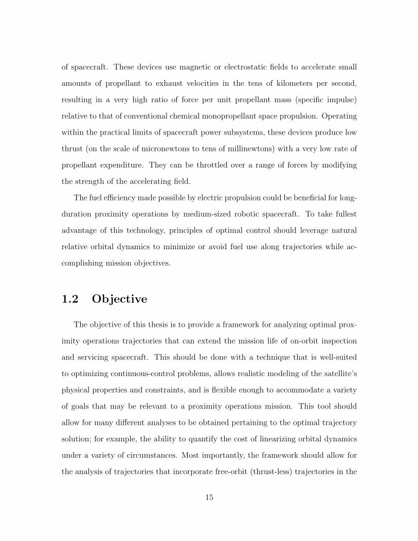
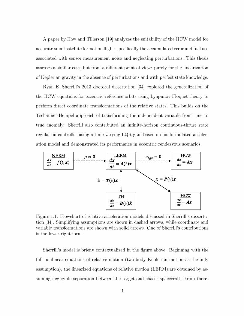
Ryan E. Sherrill’s 2013 doctoral dissertation [34] explored the generalization of

the HCW equations for eccentric reference orbits using Lyapunov-Floquet theory to

perform direct coordinate transformations of the relative states. This builds on the

Tschauner-Hempel approach of transforming the independent variable from time to

true anomaly. Sherrill also contributed an infinite-horizon continuous-thrust state

regulation controller using a time-varying LQR gain based on his formulated acceler-

ation model and demonstrated its performance in eccentric rendezvous scenarios.

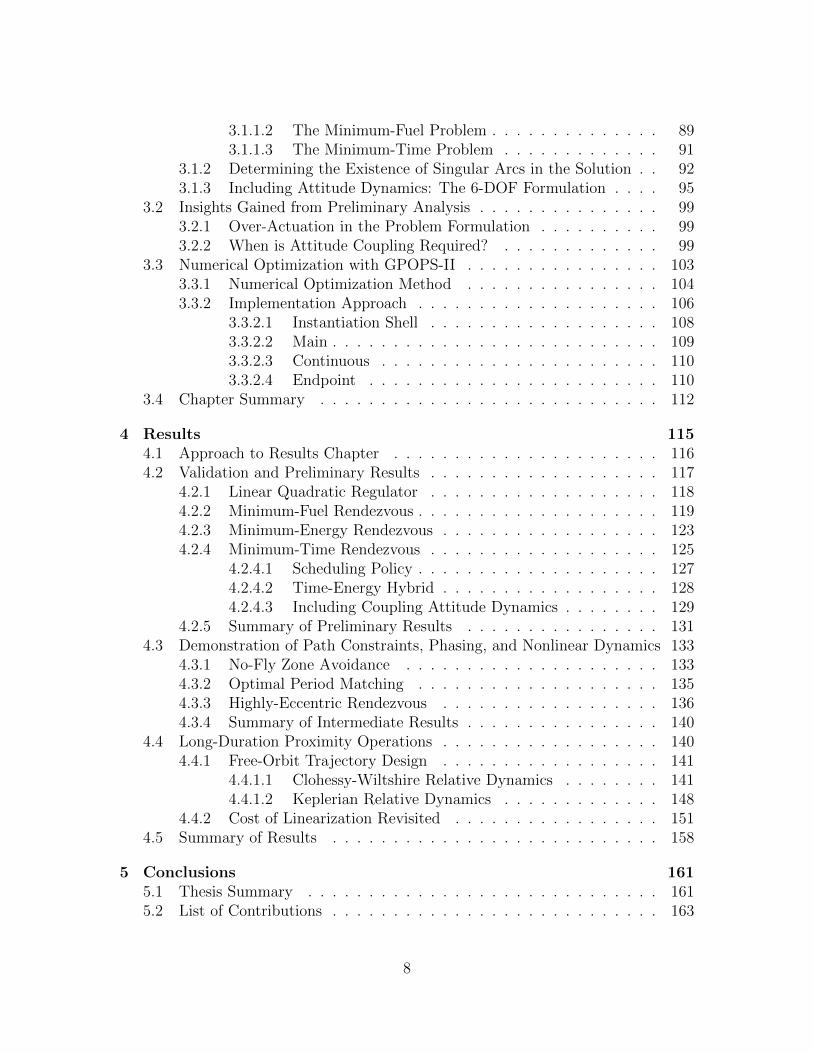
Figure 1.1: Flowchart of relative acceleration models discussed in Sherrill’s disserta-tion [34]. Simplifying assumptions are shown in dashed arrows, while coordinate andvariable transformations are shown with solid arrows. One of Sherrill’s contributionsis the lower-right form.

Sherrill’s model is briefly contextualized in the figure above. Beginning with the

full nonlinear equations of relative motion (two-body Keplerian motion as the only

assumption), the linearized equations of relative motion (LERM) are obtained by as-

suming negligible separation between the target and chaser spacecraft. From there,

19

the Hill-Clohessy-Wiltshire (HCW) model is arrived at by assuming a circular refer-

ence orbit; alternatively, changing the independent variable to true anomaly results in

the Tschauner-Hempel model. Sherrill’s model is obtained with both the independent

variable change and a coordinate transformation using Lyapunov-Floquet techniques.

Sherrill also compared periodic motion between the Keplerian model and HCW

model, and noted that a major component of error between the trajectories is caused

by rate of motion along the trajectory, not just the difference in shape. However,

most of his analysis was limited to comparisons with his generalized model, which

still makes the simplifying assumption of negligible chaser range. His optimal con-

trol analysis was also limited to the infinite-horizon LQR rendezvous case, and did

not consider insertion to or phasing between periodic trajectories. Further research

on continuous-thrust trajectory control using higher-fidelity models was identified by

Sherrill as future work. Based in part on this recommendation, the trajectory opti-

mization carried out in this thesis explores bounded continuous-thrust optimal control

solutions with the nonlinear equation of motion.

Karlgaard’s 2001 master’s thesis [24] develops a second-order linearization of the

nonlinear Keplerian relative motion equations which is similar to the HCW model, but

truncates a Taylor series approximation (see subsection 2.1.3) following the quadratic

term instead of the linear term. He also performs a systematic fidelity comparison of

his second-order linearization to both the Keplerian and HCW models. Woffinden and

Geller [41] presented an analytical sufficient condition for the observability of range

from angles-only bearing measurements in the linear HCW model, which requires the

chaser to actively maneuver relative to the target to be ranged. Gaias, et al. [14]

concur with Woffinden and Geller on the need for calibrated maneuvers to obtain

angles-only range observability, though their analysis used differential orbital elements

as the relative motion state (but still within the HCW linearization). A doctoral

20

dissertation soon to be published by M. Yates [42] explores how passive angles-only

range observability within the resolution capabilities of current star camera technology

can be obtained by considering natural nonlinearities and perturbations within the

relative motion model. While angles-only navigation is not discussed in this thesis,

obtaining passive range observability is an example of an additional motivation for

the consideration of higher-fidelity relative motion models for on-orbit inspection and

proximity operations.

1.4.3 Proximity Operations with Free-Orbit Trajectories

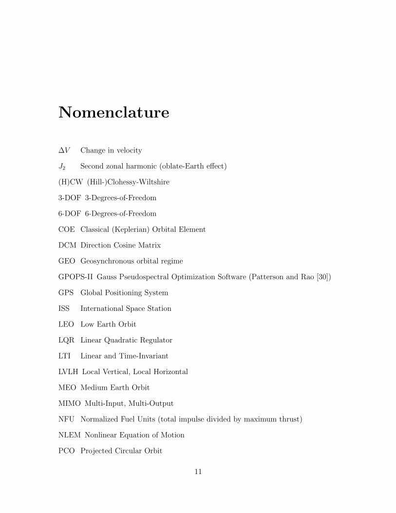
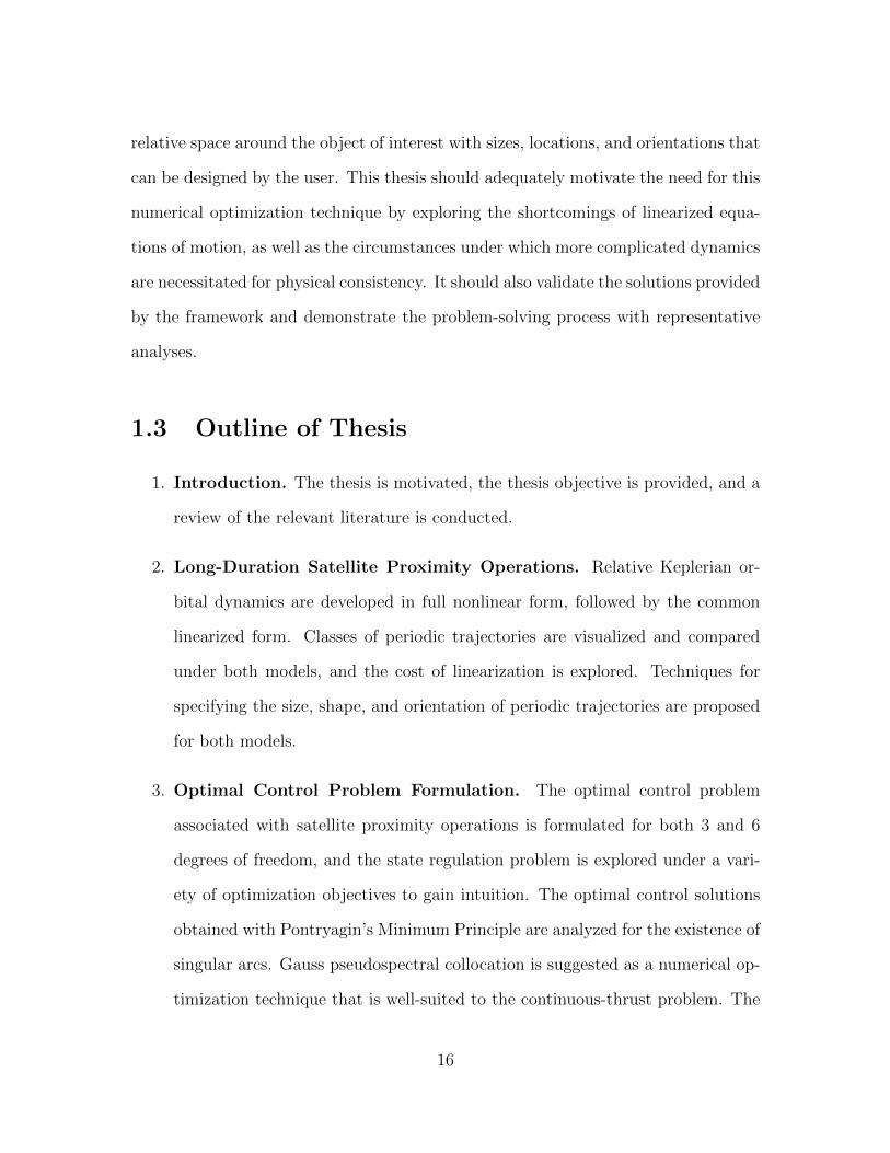
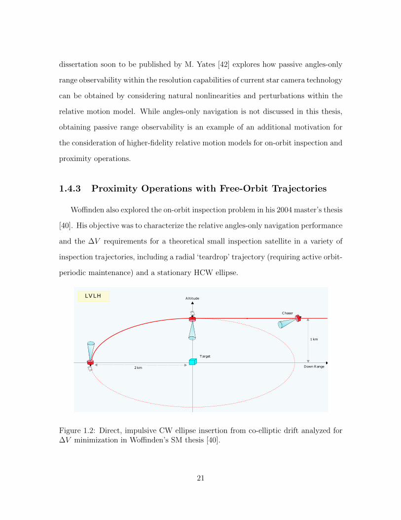
Woffinden also explored the on-orbit inspection problem in his 2004 master’s thesis

[40]. His objective was to characterize the relative angles-only navigation performance

and the ∆V requirements for a theoretical small inspection satellite in a variety of

inspection trajectories, including a radial ‘teardrop’ trajectory (requiring active orbit-

periodic maintenance) and a stationary HCW ellipse.

Target

Chaser

1 km

A ltitude

Down Range

LVLH

2km

Figure 1.2: Direct, impulsive CW ellipse insertion from co-elliptic drift analyzed for∆V minimization in Woffinden’s SM thesis [40].

21

Woffinden’s analysis of HCW ellipse insertion trajectories only considers impulsive-

thrust maneuvers, as shown in Figure 1.2. He identified as future work the need for

a flight algorithm that can flexibly transfer the chaser from anywhere in the rela-

tive state space to any desired relative motion trajectory. While this thesis considers

continuous-thrust paradigms instead of impulsive transfers, it does address techniques

for parameterizing desired relative motion characteristics in terms of the relative states

to work toward this flexibility.

In a 2005 NASA Goddard report, Naasz [29] was motivated by the proposed mis-

sion of the Hubble Robotic Vehicle to conduct unmanned inspection and servicing of

the Hubble Space Telescope (which was canceled in the same year at the recommen-

dation of studies indicating that it would not have been feasible [16]). Naasz explored

proximity operations from the point of view of the ‘safety ellipse’ concept (termed by

Wigbert Fehse in his text, Automated Rendezvous and Docking of Spacecraft [12]).

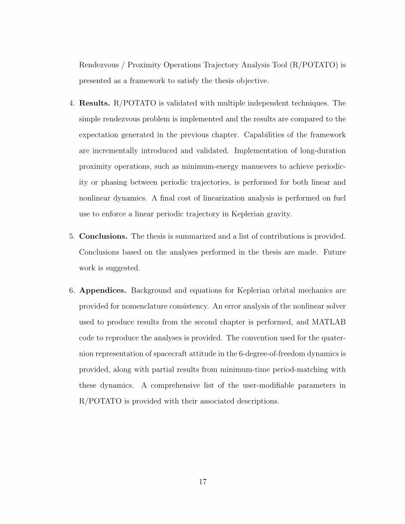
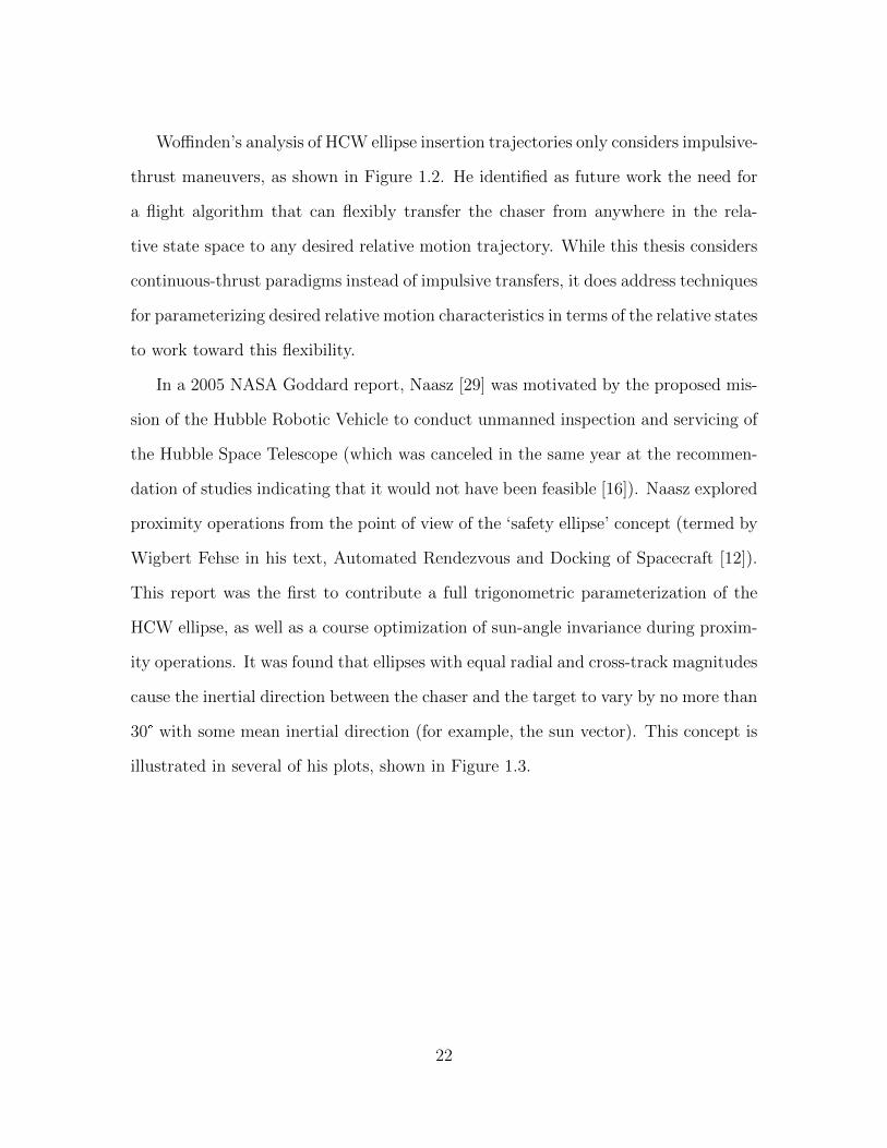
This report was the first to contribute a full trigonometric parameterization of the

HCW ellipse, as well as a course optimization of sun-angle invariance during proxim-

ity operations. It was found that ellipses with equal radial and cross-track magnitudes

cause the inertial direction between the chaser and the target to vary by no more than

30° with some mean inertial direction (for example, the sun vector). This concept is

illustrated in several of his plots, shown in Figure 1.3.

22

Figure 1.3: Safety ellipse motion in the inertial frame coarsely optimized for sun anglevariation by Naasz [29], obtaining less than 30° of variation for a static CW ellipsewith equal radial and cross-track amplitudes.

Naasz also anticipated that oblate-Earth effects would result in the in-track drift

of the ellipse’s center, for which he recommended periodic impulsive maintenance or

re-initialization of the ellipse. For future work, further discussion of the effects of

other perturbations on relative motion was suggested. This thesis focuses in part on

the ‘pseudo-perturbation’ arising as the result of linearizing Keplerian gravity, which

(unlike other perturbations) could be avoided by utilizing higher-fidelity motion mod-

els in mission planning and for trajectory design and maintenance. While J2 effects

were not modeled in R/POTATO, inclusion of this effect and other deterministic

perturbations would be straightforwardly implemented in the Continuous function.

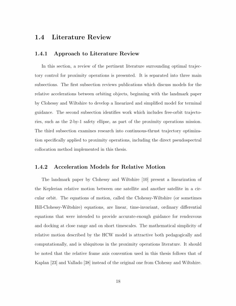
In another NASA Goddard report published in 2011 [2], Barbee and various other

authors (including Naasz) refocused the proximity operations mission design concept

on non-cooperative targets at geosynchronous orbit. They developed an RPO mission

23

framework for a hypothetical autonomous servicer to safely rendezvous with, inspect,

capture, and dispose of a malfunctioning GEO satellite into a super-synchronous

graveyard orbit. The rendezvous strategy involved repeated Hohmann raises from

lower co-elliptic orbits, as shown in Figure 1.4.

Figure 1.4: Impulsive-thrust RPO strategy developed by Barbee, et al. [2] that in-cludes periods of thrust-less co-elliptic drift with intermittent Hohmann raises, fol-lowed by an insertion into a safety ellipse using targeting techniques.

Unlike Woffinden’s CW ellipse insertion, the strategy described by Barbee, et al.

use Lambert or CW targeting techniques for final insertion from the last co-elliptic

segment. Similar to Woffinden, however, the RPO strategy is designed based on the

impulsive-thrust paradigm. Discussion of free-orbit ellipse design follows from and

builds upon Naasz’s original work, and features the sun-angle-optimized design as an

example. ‘Walking’ safety ellipses are discussed as a technique for safely approaching

24

the target along the in-track axis; these corkscrew-like trajectories are similar to

offset and inclined ellipses, but have non-zero in-track drift, and as a result are also

slightly offset radially from the in-track axis. The authors identify several avenues for

future work: development of thruster selection algorithms for proximity operations,

implementation in a high-fidelity 6-degree-of-freedom simulation, and consideration

of low-thrust solar electric propulsion paradigms for proximity operations missions.

This thesis touches on all of these items.

A 2011 master’s thesis by James Meub [27] investigates the feasibility of LEO

inspection using low-thrust cold-gas propulsion, proposing the M-SAT mission as a

platform to demonstrate inspection operations. The author specifies desired inspec-

tion trajectories in the HCW model by satisfying a linear periodicity condition, and

re-expresses the solution’s periodic motion in phase-amplitude form. A similar ap-

proach is taken in this thesis for the specification of HCW ellipse orientation.

A 2002 paper by Inalhan, Tillerson, and How [20] presents a strategy to initialize

periodic trajectories in eccentric reference orbits in the Tschauner-Hempel model for

the purpose of sparse-aperture synthesis satellite formation flight. By comparing with

the HCW model, the authors concluded that ignoring reference orbit eccentricity on

the order of e ≈ 10−3 for a 1-kilometer aperture can be a dominant source of modeling

error on par with ignoring J2 perturbations. A similar analysis was carried out in

this thesis; however, comparison was drawn between the full nonlinear relative motion

and the HCW model.

A paper by Schaub, et al. [32] contributes a spacecraft formation flight nonlinear

feedback law based on differential mean orbital elements of the spacecraft, for which

they proved Lyapunov stability. Their method makes no linearizing assumptions

about relative motion, and they attempt to control the chaser’s orbital elements to

an orbit that is J2-invariant with respect to the target’s orbit based on a set of first-

25

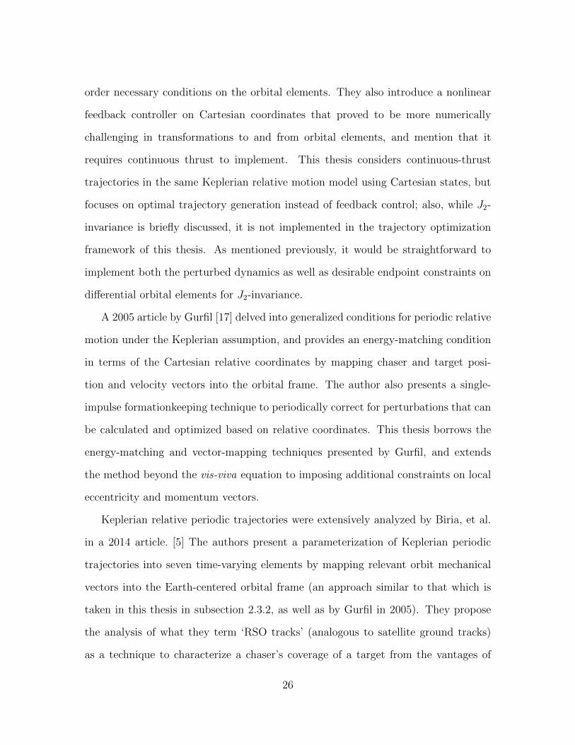
order necessary conditions on the orbital elements. They also introduce a nonlinear

feedback controller on Cartesian coordinates that proved to be more numerically

challenging in transformations to and from orbital elements, and mention that it

requires continuous thrust to implement. This thesis considers continuous-thrust

trajectories in the same Keplerian relative motion model using Cartesian states, but

focuses on optimal trajectory generation instead of feedback control; also, while J2-

invariance is briefly discussed, it is not implemented in the trajectory optimization

framework of this thesis. As mentioned previously, it would be straightforward to

implement both the perturbed dynamics as well as desirable endpoint constraints on

differential orbital elements for J2-invariance.

A 2005 article by Gurfil [17] delved into generalized conditions for periodic relative

motion under the Keplerian assumption, and provides an energy-matching condition

in terms of the Cartesian relative coordinates by mapping chaser and target posi-

tion and velocity vectors into the orbital frame. The author also presents a single-

impulse formationkeeping technique to periodically correct for perturbations that can

be calculated and optimized based on relative coordinates. This thesis borrows the

energy-matching and vector-mapping techniques presented by Gurfil, and extends

the method beyond the vis-viva equation to imposing additional constraints on local

eccentricity and momentum vectors.

Keplerian relative periodic trajectories were extensively analyzed by Biria, et al.

in a 2014 article. [5] The authors present a parameterization of Keplerian periodic

trajectories into seven time-varying elements by mapping relevant orbit mechanical

vectors into the Earth-centered orbital frame (an approach similar to that which is

taken in this thesis in subsection 2.3.2, as well as by Gurfil in 2005). They propose

the analysis of what they term ‘RSO tracks’ (analogous to satellite ground tracks)

as a technique to characterize a chaser’s coverage of a target from the vantages of

26

a periodic circumnavigating inspection trajectory, and assert that the most valuable

inspection trajectories have uniformly dense RSO tracks over the target’s surface area.

This implies a need to be able to adequately design relative trajectories to accomplish

surveying coverage objectives, which Chapter 2 explores. Additionally, the authors

perform an analysis of the validity of the Tschauner-Hempel equations, and note that

error accrues significantly for relative orbits with requirements on large separations,

which they identify as a common situation in the realm of space-based situational

awareness applications. This thesis reaches a similar conclusion as a result of the

various ‘cost of linearization’ analyses performed.

1.4.4 Continuous-Thrust Trajectory Optimization for Prox-

imity Operations

An article by Zhou, et al. [43] presents a 2π-periodic Lyapunov differential equa-

tion approach to linear quadratic regulation with eccentric targets. The decoupling

of in-plane and out-of-plane motion in the Tschauner-Hempel dynamical model is ex-

ploited, and it is shown that instead of solving a nonlinear Ricatti differential equation,

one need only solve a simpler linear Lyapunov differential equation to obtain a time-

varying LQR state feedback gain matrix. It was further shown that the controller

is semi-globally asymptotically stable for a bounded-control and bounded-energy for-

mulation. A periodic generator numerical technique is proposed to efficiently solve

the Lyapunov equation on-line. Although the solver used in this thesis is not suitable

for state feedback control or on-line implementation, it solves linear quadratic regu-

lation problems in several seconds with a higher-fidelity acceleration model than the

Tschauner-Hempel equations. This article also only analyzes the regulation problem,

and does not consider free-orbit motion as a desirable destination dynamics.

27

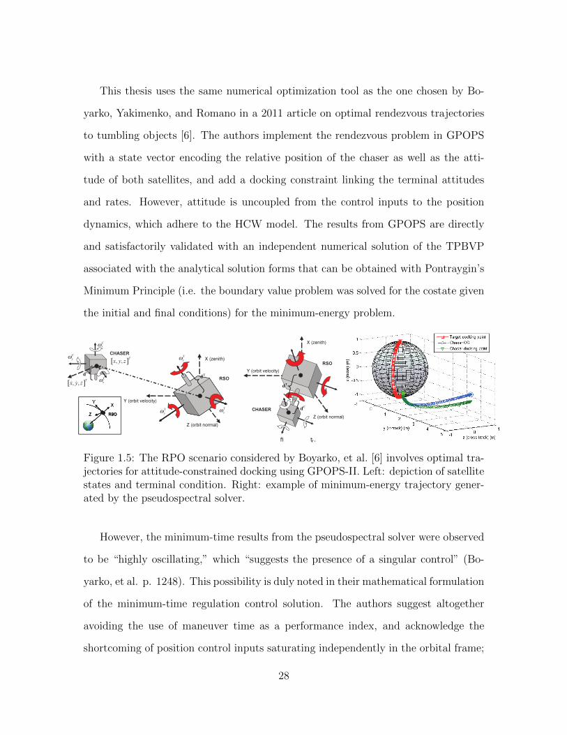
This thesis uses the same numerical optimization tool as the one chosen by Bo-

yarko, Yakimenko, and Romano in a 2011 article on optimal rendezvous trajectories

to tumbling objects [6]. The authors implement the rendezvous problem in GPOPS

with a state vector encoding the relative position of the chaser as well as the atti-

tude of both satellites, and add a docking constraint linking the terminal attitudes

and rates. However, attitude is uncoupled from the control inputs to the position

dynamics, which adhere to the HCW model. The results from GPOPS are directly

and satisfactorily validated with an independent numerical solution of the TPBVP

associated with the analytical solution forms that can be obtained with Pontraygin’s

Minimum Principle (i.e. the boundary value problem was solved for the costate given

the initial and final conditions) for the minimum-energy problem.

fi tf .

Figure 1.5: The RPO scenario considered by Boyarko, et al. [6] involves optimal tra-jectories for attitude-constrained docking using GPOPS-II. Left: depiction of satellitestates and terminal condition. Right: example of minimum-energy trajectory gener-ated by the pseudospectral solver.

However, the minimum-time results from the pseudospectral solver were observed

to be “highly oscillating,” which “suggests the presence of a singular control” (Bo-

yarko, et al. p. 1248). This possibility is duly noted in their mathematical formulation

of the minimum-time regulation control solution. The authors suggest altogether

avoiding the use of maneuver time as a performance index, and acknowledge the

shortcoming of position control inputs saturating independently in the orbital frame;

28

future work is recommended to address these areas. Much of the third chapter of

this thesis is focused on the identification of the singular control which these authors

identified, the need for coupling between attitude and position in the dynamics for

the minimum-time problem (and conversely the absence of this need for other objec-

tives under certain conditions), as well as other mitigation techniques to recapture

uniqueness in the solution.

Boyarko’s 2010 doctoral dissertation [7] considers the same 20-state rendezvous

problem, and contributes a novel trajectory generation method using inverse dynamics

in the virtual domain. Unlike the results obtained from his GPOPS implementation,

the new method is rapid enough to be run on-line. Though this technique sacrifices the

global optimality of the solution, Boyarko argues that the computation time regained

is an acceptable trade. This dissertation also notes the existence of the possibility of

singular control in the minimum-time problem, but goes on to report that it is resolved

by considering body-mounted thruster saturation instead of orbital frame saturation

(in essence, coupling the dynamics). A shortcoming of both this dissertation and

the journal paper is a small (but important) error that appears in the definition

of the forced HCW dynamics: the relative accelerations due to linearized orbital

mechanics are divided through by vehicle mass. This has the effect of artificially

‘raising’ the target orbit by uniformly downscaling orbital rate; however, this detail

had no detrimental impact on the findings in either publication.

A 2006 doctoral dissertation by Bevilacqua [4], who studied partly under the men-

torship of Romano and Yakimenko, focused on control optimization for rendezvous

and docking in the HCW model with a variety of techniques that could be imple-

mented on-line. As a secondary topic, the author used a genetic algorithm optimizer

to identify periodic or bounded projected circular orbit (PCO) relative motion tra-

jectories in the presence of J2 and drag perturbations to maximally exploit orbital

29

dynamics for efficient formation flight. The author found it necessary to extend

the first-order conditions for J2-invariance given by Schaub, et al. [32] to a set of

second-order conditions to achieve satisfactorily stationary trajectories in nonlinear

propagation. Bevilacqua’s genetic algorithm identified invariance near the critical

inclination as expected, as well as at another unexpected inclination of 49.11°. The

author recommended that future analysis be performed to determine why invariance

could be observed at this inclination, which was carried out by Vadali, et al. [37] and

Izzo, et al. [21]. It was determined that the specific combination of the target’s orbital

elements combined with the specified PCO differential elements resulted in bounded

in-track drift at the inclination of 49.11°. This type of analysis, but with scope ex-

panded from PCOs to any circumnavigating motion, is an example of a research

question that could be explored using the tool presented in this thesis, R/POTATO,

with only slight modification.

Richard Epenoy’s 2011 article [11] examines the minimum-fuel rendezvous prob-

lem for a chaser with constrained continuous thrust using the Tschauner-Hempel

motion model. The optimization problem is posed as a nonlinear program with an

added collision-avoidance inequality constraint. Epenoy designs an efficient numer-

ical technique for solving the constrained problem by instead solving a sequence of

unconstrained (i.e., without enforcing collision avoidance) problems, the solutions for

which he shows convergence to the constrained problem. Since he looked only at the

minimum-fuel problem, the optimal control was identified to be of the ‘bang-off-bang’

paradigm discussed in Chapter 3 based on Pontryagin’s Minimum Principle. Epenoy

noted that transcription techniques, like shooting and collocation methods, are ill-

suited to direct optimizaion of the control thrust in the minimum-fuel problem as a

result of the discontinuities and sizable singular interval. This thesis reaches a similar

conclusion for the analysis of the minimum-fuel problem with Gauss pseudospectral

30

collocation, and determines that the minimum-energy objective produces much more

satisfying numerical results, as well as being more applicable to the electric propulsion

paradigm.

1.4.5 Summary of Review

This literature review focused on research pertaining to three main areas: devel-

opment and analysis of relative motion models of varying fidelity and the impact on

relevant mission objectives, the characterization and implementation of free-orbit tra-

jectories for inspection and formation flight, and techniques for proximity operations

trajectory optimization. Based on insights gained from the reviewed literature as

well as an intersection of their suggested future work, this thesis sets out to develop a

framework for analyzing optimal proximity operations trajectories that can be flexibly

obtained for very general problems. For example, problems with arbitrarily nonlinear

and potentially attitude-coupled dynamics, various optimization goals ranging from

state regulation to ellipse insertion, precise specification of a range of periodic trajec-

tories, various optimization objectives, and various vehicle properties with physical

constraints. This objective is realized in the contribution of R/POTATO, which is

validated and demonstrated in the results of several analyses.

It is important to note, however, that R/POTATO is a numerical tool for under-

standing and analyzing optimal proximity operations trajectories, not for generating

them in an on-line or in a closed-loop fashion onboard an autonomous agent. At best,

the results are open-loop optimal control laws assuming perfect state knowledge, and

are certainly not robust to the range of real challenges associated with flight imple-

mentations that demand sophisticated reference-tracking control and state estimation

techniques. An in-depth review of various reference-tracking controllers across the en-

31

tire range of the proximity operations problem in the presence of both measurement

uncertainty and uncertain events can be found in the concurrently published doctoral

dissertation by C. Jewison. [22]

32

Chapter 2

Long-Duration Satellite ProximityOperations

This chapter develops the conceptual language and mathematical basis for ana-

lyzing long-duration satellite proximity operations. Throughout the chapter, a fun-

damental level of knowledge of orbital dynamics is assumed; Appendix A provides

an introduction to these concepts and equations for the reader’s convenience and for

consistency in nomenclature.

Emphasis is given on the classical development [10] of the linearized Hill-Clohessy-

Wiltshire equations of relative motion from the full, nonlinear form [17] [34] that can

be obtained from kinematics and the Two-Body Equation, with scrutiny on the cost

of making the linearizing assumptions in terms of a quantitative comparison under

a variety of circumstances. While it is straightforward to obtain solutions from the

linearized dynamics, it is necessary to use a nonlinear solver for the other set of

dynamics; MATLAB’s ode113 solver was chosen for this task. Appendix B elaborates

the reasoning behind this choice, along with a comparison to the state-of-the-art

benchmark Two-Body propagation tool furnished by Systems Tool Kit (STK) [36].

Classes of relative motion are briefly described, and the linearization error is ana-

lyzed for some simple cases. More time is spent on describing periodic circumnavigat-

33

ing trajectories in the relative space around a target RSO in terms of the cartesian

relative coordinates, treating the spatial specification of these relative trajectories

as a set of path constraints over these six variables. This is straightforward for the

Clohessy-Wiltshire dynamics, which predicts trajectories that can essentially be posed

as geometric constraints; however, the irregularly-shaped true nonlinear trajectories

warrant an approach that constrains differential Keplerian elements (expressed in the

cartesian relative frame) to specify the desired size, shape, and location of the periodic

trajectory.

Chapter 3, which details the implementation of the optimal proximity operations

problem in a general numerical optimization tool (GPOPS-II [30]), is motivated in

part by the findings of this chapter: for long-duration proximity operations, there is a

need to analyze the optimal control problem for higher-fidelity nonlinear astrodynam-

ical equations of relative motion, and a desire to control to a free-orbit (zero-thrust)

periodic trajectory instead of to a point in space. In essence, both bring more real-

ism or flexibility to the problem, yet introduce nonlinearities to the plant dynamics

or terminal conditions for which obtaining an analytical solution may be tedious or

intractable.

2.1 Relative Orbital Dynamics

Proximity operations between satellites requires an accurate representation of the

motion of one satellite with respect to another. Developing the equations of rela-

tive motion involves a vector analysis of the two satellites. This subsection begins

by describing the relative motion reference frame, proceeds with developing the full

nonlinear equations of relative motion, then makes various simplifying assumptions

to arrive at the linear and time-invariant Clohessy-Wiltshire equations of motion [10].

34

2.1.1 The LVLH Coordinate Frame

A common coordinate frame used for describing the relative motion between two

spacecraft is a target-centered ‘local vertical, local horizontal’ (LVLH) reference frame.

The convention for axis assignment used in this thesis is the same that is used by

Vallado [38] and Kaplan [23]. The x (sometimes called ‘radial’ or ‘R-bar’) coordinate is

the local vertical, and is positive along the target’s orbital radius vector pointing away

from the Earth’s center of mass. The y (also called ‘in-track’ or ‘V-bar’) coordinate

is the local horizontal, and is perpendicular to the radial direction in the plane of

the orbit in the direction of motion; for circular orbits, this direction is the same as

the velocity vector. The z or ‘cross-track’ coordinate is positive along the target-

centered vector parallel to the target’s orbital angular momentum vector (completing

the right-handed coordinate frame). Sometimes, the axes are named ‘RSW’ instead

of ‘XYZ.’ This is not the only coordinate convention used for describing relative

orbital dynamics, but it is one of the most common and easy to work with due to

the mnemonic value of having the three axes align with three important vectors from

fundamental orbital dynamics (x ‖ r, y ‖ v for circular orbits, and z ‖ h). Of course,

the center of the LVLH frame need not be on an actual target satellite; it may be any

fixed point of interest along some orbital trajectory (a ‘reference’ trajectory).

2.1.2 The Full Keplerian Nonlinear Equations of Relative

Motion

This subsection develops the laws of relative motion between two spacecraft gov-

erned by Keplerian gravitational dynamics. This development parallels the one pro-

vided by Sherrill’s dissertation [34]. The terms “chaser” and “target” are to be used

to describe the objects of interest in this problem, where the chaser is displaced by

35

Earth-Centered Inertial Frame(fixed)

r

LVLH Frame (rotating)Orbital

Trajectory

K

J

I

z

y x

Figure 2.1: Illustration of the LVLH reference frame.

some amount in the LVLH coordinate frame from the target, and the target is placed

at the center of the LVLH frame. With vector addition, the following relationship

can be written:

rch = rtgt + ρ

Where ρ is the range vector of the chaser in the target-centered LVLH frame:

ρ =

x

y

z

To obtain the chaser’s velocity in the inertial frame, its position vector is differentiated

with respect to time:

˙rch = ˙rtgt + ˙ρ+ ω × ρ

36

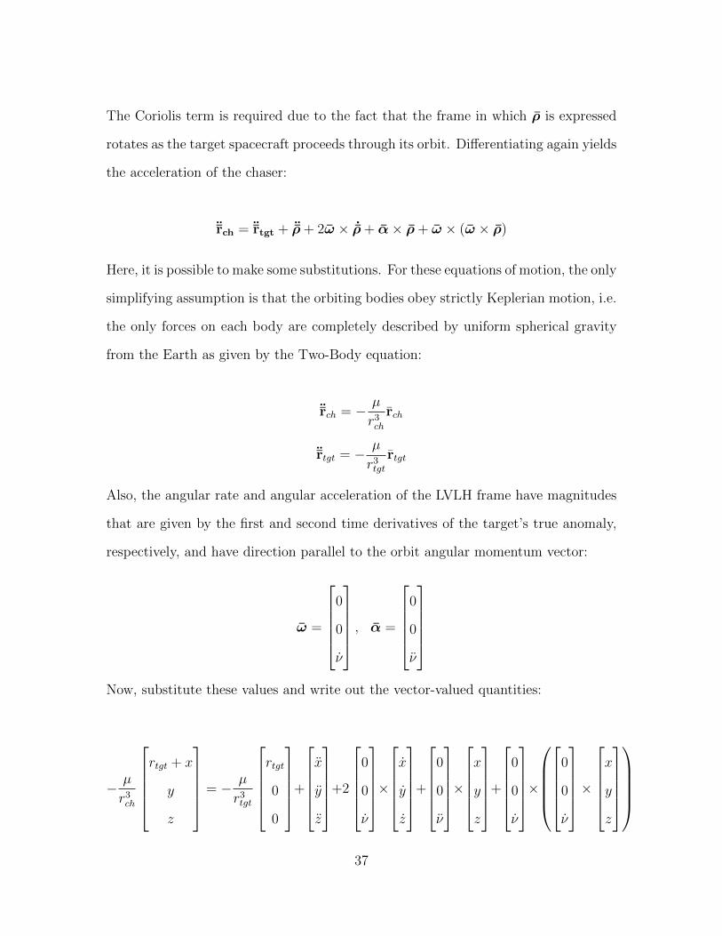
The Coriolis term is required due to the fact that the frame in which ρ is expressed

rotates as the target spacecraft proceeds through its orbit. Differentiating again yields

the acceleration of the chaser:

¨rch = ¨rtgt + ¨ρ+ 2ω × ˙ρ+ α× ρ+ ω × (ω × ρ)

Here, it is possible to make some substitutions. For these equations of motion, the only

simplifying assumption is that the orbiting bodies obey strictly Keplerian motion, i.e.

the only forces on each body are completely described by uniform spherical gravity

from the Earth as given by the Two-Body equation:

¨rch = − µ

r3chrch

¨rtgt = − µ

r3tgtrtgt

Also, the angular rate and angular acceleration of the LVLH frame have magnitudes

that are given by the first and second time derivatives of the target’s true anomaly,

respectively, and have direction parallel to the orbit angular momentum vector:

ω =

0

0

ν

, α =

0

0

ν

Now, substitute these values and write out the vector-valued quantities:

− µ

r3ch

rtgt + x

y

z

= − µ

r3tgt

rtgt

0

0

+

x

y

z

+2

0

0

ν

×x

y

z

+

0

0

ν

×x

y

z

+

0

0

ν

×

0

0

ν

×x

y

z

37

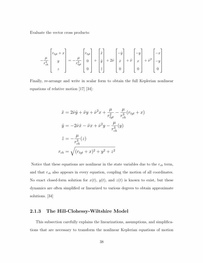
Evaluate the vector cross products:

− µ

r3ch

rtgt + x

y

z

= − µ

r3tgt

rtgt

0

0

+

x

y

z

+ 2ν

−y

x

0

+ ν

−y

x

0

+ ν2

−x

−y

0

Finally, re-arrange and write in scalar form to obtain the full Keplerian nonlinear

equations of relative motion [17] [34]:

x = 2νy + νy + ν2x+µ

r2tgt− µ

r3ch(rtgt + x)

y = −2νx− νx+ ν2y − µ

r3ch(y)

z = − µ

r3ch(z)

rch =√

(rtgt + x)2 + y2 + z2

Notice that these equations are nonlinear in the state variables due to the rch term,

and that rch also appears in every equation, coupling the motion of all coordinates.

No exact closed-form solution for x(t), y(t), and z(t) is known to exist, but these

dynamics are often simplified or linearized to various degrees to obtain approximate

solutions. [34]

2.1.3 The Hill-Clohessy-Wiltshire Model

This subsection carefully explains the linearizations, assumptions, and simplifica-

tions that are necessary to transform the nonlinear Keplerian equations of motion

38

into the commonly-used Clohessy-Wiltshire equations. This is done in the interest of

illustrating the causes of linearization error and why its accumulation is more serious

for long-duration proximity operations at range.

Linearization of the Keplerian equations of relative motion results in a more an-

alytically tractable motion model. Linearization propagates the assumption that the

chaser and target are relatively close to each other such that the difference between

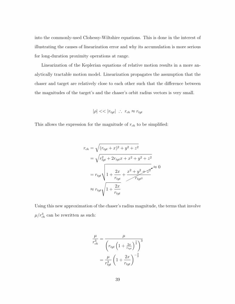
the magnitudes of the target’s and the chaser’s orbit radius vectors is very small.

|ρ| << |rtgt| ∴ rch ≈ rtgt

This allows the expression for the magnitude of rch to be simplified:

rch =√

(rtgt + x)2 + y2 + z2

=√r2tgt + 2rtgtx+ x2 + y2 + z2

= rtgt

√√√√1 +

2x

rtgt+

*≈ 0

x2 + y2 + z2

rtgt2

≈ rtgt

√1 +

2x

rtgt

Using this new approximation of the chaser’s radius magnitude, the terms that involve

µ/r3ch can be rewritten as such:

µ

r3ch=

µ(rtgt

(1 + 2x

rtgt

) 12

)3

=µ

r3tgt

(1 +

2x

rtgt

)− 32

39

This term is still nonlinear in the x coordinate. This can be dealt with by using a

binomial series expansion of the form:

(1 + a)n = 1 + nx+n(n− 1)a2

2!+ ...

Under this series expansion, the binomial of interest can be rewritten:

(1 +

2x

rtgt

)− 32

= 1− 3x

rtgt+

15x2

2r2tgt+ ...

Because the goal is to reach an expression that is linear in the state variable, it is nec-

essary to truncate the series after the first-order term, invoking the same assumption

that x is small relative to rtgt:

(1 +

2x

rtgt

)− 32

≈ 1− 3x

rtgt

Substituting this back into the equations of motion and invoking the original assump-

tion in several places:

40

x = 2νy + νy + ν2x+µ

r2tgt− µ

r3tgt

(1− 3x

rtgt

)(rtgt + x)

= 2νy + νy + ν2x+µ

r2tgt− µ

r3tgt

rtgt + x− 3x−7≈ 0

3x2

rtgt

= 2νy + νy + ν2x+

µ

r2tgt−µ

r2tgt+ 2

µ

r3tgtx

= 2νy + νy + ν2x+ 2µ

r3tgtx

y = −2νx− νx+ ν2x− µ

r3tgt

1−7≈ 0

3x

rtgt

(y)

= −2νx− νx+ ν2x− µ

r3tgty

z = − µ

r3tgt

1−7≈ 0

3x

rtgt

(z)

= − µ

r3tgtz

At this point, the equations of motion have been linearized, but they are not time

invariant unless the target is in a perfectly circular orbit. It is still possible to obtain

a closed-form solution to the above linear ODEs without making this assumption,

but it is necessary to perform a coordinate transformation such that time is replaced

as the independent variable by true anomaly. This is called the Tschauner-Hempel

solution. [34] In the interest of restricting the scope and complexity of the upcoming

optimal control theory analysis to LTI dynamics, the assumption is made that the

target’s orbit has an eccentricity of zero:

41

ν = 0, ν = n,µ

r3tgt= ν2 = n2

The result is a relatively simple system of three linear and time-invariant second-order

ODEs, known as Hill’s equations or the Clohessy-Wiltshire equations of motion:

x = 2ny + 3n2x

y = −2nx

z = −n2z

Notice that motion in the orbital plane is coupled, but cross-plane motion is not (z

dynamics are analogous to a simple harmonic oscillator). This is due to the fact that

the target-centered reference frame is itself accelerating, but its acceleration (which

comprises both Coriolis and centripetal effects) has components only in the orbital

plane.

The Clohessy-Wiltshire equations can be solved analytically for closed-form posi-

tion and velocity solutions using a variety of techniques. Vallado [38] demonstrates

a Laplace transform approach toward solving the system of differential equations to

obtain these solutions:

42

x(t) = −(

3x0 +2

ny0

)cos (nt) +

(1

nx0

)sin (nt) +

(4x0 +

2

ny0

)y(t) =

(2

nx0

)cos (nt) +

(6x0 +

4

ny0

)sin (nt)− (6nx0 + 3y0) t+

(y0 −

2

nx0

)z(t) = (z0) cos (nt) +

(1

nz0

)sin (nt)

x(t) = (x0) cos (nt) + (3nx0 + 2y0) sin (nt)

y(t) = (6nx0 + 4y0) cos (nt)− (2x0) sin (nt)− (6nx0 + 3y0)

z(t) = (z0) cos (nt)− (nz0) sin (nt)

2.2 Comparison of Classes of Nonlinear and Lin-

earized Relative Motion Trajectories

Summarized below is the list of assumptions that were required to reach the

Clohessy-Wiltshire equations and their solutions from the starting point of the Kep-

lerian nonlinear equations of relative motion:

Chaser and target are relatively close together: |ρ| << |rtgt| ∴ rch ≈ rtgt

In the expression for rch:ρ2

r2tgt≈ 0

In the expression for x: 3x2

rtgt≈ 0

In the expression for y: 3xrtgt≈ 0

In the expression for z: 3xrtgt≈ 0

The binomial series expansion is truncated after the first-order term:(1 + 2x

rtgt

)− 32 ≈ 1− 3x

rtgt

The target’s orbit is perfectly circular.

43

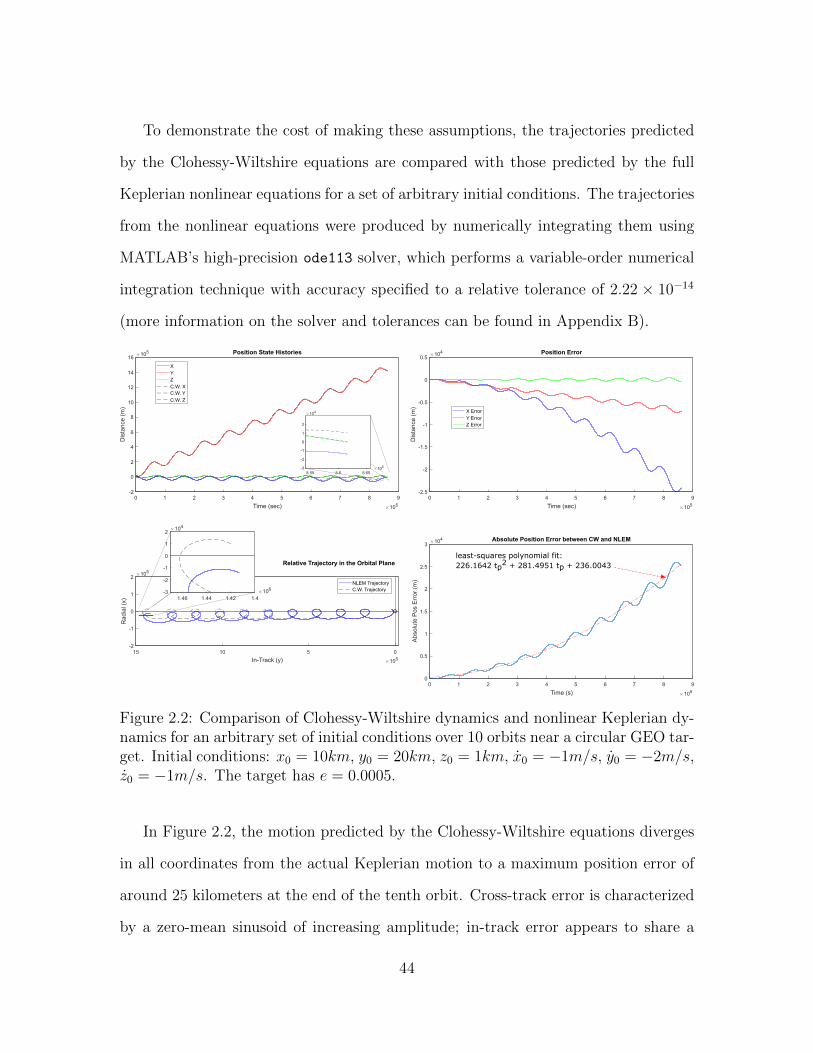
To demonstrate the cost of making these assumptions, the trajectories predicted

by the Clohessy-Wiltshire equations are compared with those predicted by the full

Keplerian nonlinear equations for a set of arbitrary initial conditions. The trajectories

from the nonlinear equations were produced by numerically integrating them using

MATLAB’s high-precision ode113 solver, which performs a variable-order numerical

integration technique with accuracy specified to a relative tolerance of 2.22 × 10−14

(more information on the solver and tolerances can be found in Appendix B).

0 1 2 3 4 5 6 7 8 9

Time (sec) 105

-2

0

2

4

6

8

10

12

14

16

Dis

tanc

e (m

)

105 Position State Histories

X

YZ

C.W. XC.W. Y

C.W. Z

0 1 2 3 4 5 6 7 8 9

Time (sec) 105

-2.5

-2

-1.5

-1

-0.5

0

0.5

Dis

tanc

e (m

)

104 Position Error

X Error

Y ErrorZ Error

-2

-1

0

1

2

Rad

ial (

x)

105

051015

In-Track (y) 105

Relative Trajectory in the Orbital Plane

NLEM TrajectoryC.W. Trajectory

0 1 2 3 4 5 6 7 8 9

Time (s) 105

0

0.5

1

1.5

2

2.5

3

Abs

olu

te P

os E

rror

(m)

104 Absolute Position Error between CW and NLEM

least-squares polynomial fit:226.1642 tp2 + 281.4951 tp + 236.0043

-3

-2

-1

0

1

2104

1.41.421.441.46106

8.55 8.6 8.65105-3

-2

-1

0

1

2

104

Figure 2.2: Comparison of Clohessy-Wiltshire dynamics and nonlinear Keplerian dy-namics for an arbitrary set of initial conditions over 10 orbits near a circular GEO tar-get. Initial conditions: x0 = 10km, y0 = 20km, z0 = 1km, x0 = −1m/s, y0 = −2m/s,z0 = −1m/s. The target has e = 0.0005.

In Figure 2.2, the motion predicted by the Clohessy-Wiltshire equations diverges

in all coordinates from the actual Keplerian motion to a maximum position error of

around 25 kilometers at the end of the tenth orbit. Cross-track error is characterized

by a zero-mean sinusoid of increasing amplitude; in-track error appears to share a

44

similar sinusoidal nature but with a mean that grows approximately linearly; radial

error grows as a sinusoid with increasing amplitude and a mean that grows faster than

linearly. In the lower-left panel, the Keplerian trajectory can be observed diverging

from the linearized trajectory (it follows the orbital trajectory, which curves down

and away from the local horizontal axis).

This seems like a large amount of error, but inspection of the state histories and

the orbital plane relative trajectory seem to indicate close agreement between the

Clohessy-Wiltshire trajectories and the true Keplerian motion. This is attributable

to the large orbital radius of the target (it is at geostationary orbit, which corresponds

to a semimajor axis of 42, 164.137 km); thus, 25 kilometers corresponds to less than

a 2% error. Although the initial conditions placed the chaser tens of kilometers away

from the target, this initial offset is less than 1/1885th of the size of the target’s

orbital radius. For certain applications, this error may be small enough to justify the

assumptions that the Clohessy-Wiltshire equations make regarding the small size of

the chaser’s range with respect to the target’s radius.

In Table 2.1, various stationary initial offsets in both the x and y coordinates are

analyzed, and the position percent error between Clohessy-Wiltshire and nonlinear

Keplerian motion is computed after 1 orbit, 3 orbits, and 10 orbits. An additional

column introduces a non-zero eccentricity into the 10-orbit error computation.

45

LEO (200 km altitude)x0(km)

y0(km)

ρ0/a % Error:1 Orbit,etgt = 0

% Error:3 Orbits,etgt = 0

% Error:10 Orbits,etgt = 0

% Error:10 Orbits,etgt = 0.0005

0.1 0 1.52× 10−5 0.0299 % 0.0867% 0.2866% 0.3401%1 0 1.52× 10−4 0.3035% 0.8671% 2.866% 2.878%10 0 1.52× 10−3 3.019% 8.645% 28.72% 28.75%0 0.1 1.52× 10−5 0.0287% 0.086% 0.2874% 0.288%0 1 1.52× 10−4 0.2874% 0.8671% 2.950% 2.957%0 10 1.52× 10−3 2.950% 9.405% 40.16% 40.29%

GEOx0(km)

y0(km)

ρ0/a % Error:1 Orbit,etgt = 0

% Error:3 Orbits,etgt = 0

% Error:10 Orbits,etgt = 0

% Error:10 Orbits,etgt = 0.0005

0.1 0 2.37× 10−6 0.0047 % 0.0134% 0.0447% 0.1818%1 0 2.37× 10−5 0.0471% 0.1347% 0.4472% 0.4854%10 0 2.37× 10−4 0.4706% 1.338% 4.471% 4.483%0 0.1 2.37× 10−6 0.0045% 0.0134% 0.0447% 0.0448%0 1 2.37× 10−5 0.0447% 0.1343% 0.4491% 0.4501%0 10 2.37× 10−4 0.4491% 1.359% 4.680% 4.691%

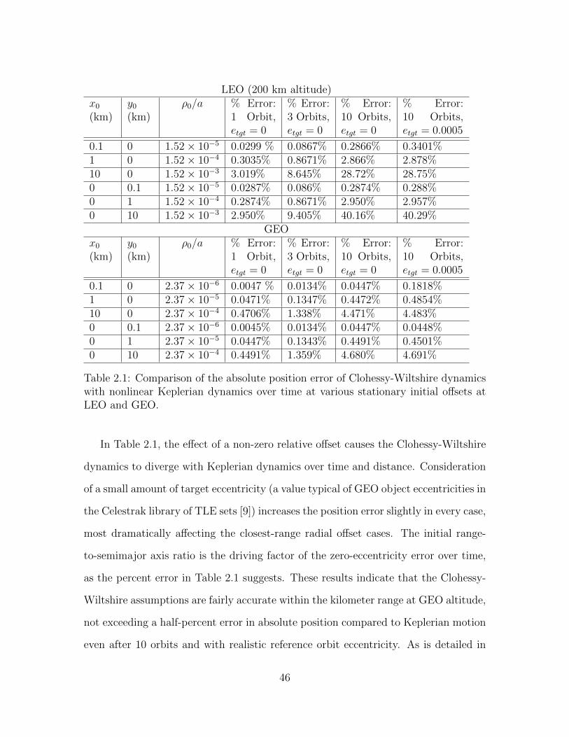
Table 2.1: Comparison of the absolute position error of Clohessy-Wiltshire dynamicswith nonlinear Keplerian dynamics over time at various stationary initial offsets atLEO and GEO.

In Table 2.1, the effect of a non-zero relative offset causes the Clohessy-Wiltshire

dynamics to diverge with Keplerian dynamics over time and distance. Consideration

of a small amount of target eccentricity (a value typical of GEO object eccentricities in

the Celestrak library of TLE sets [9]) increases the position error slightly in every case,

most dramatically affecting the closest-range radial offset cases. The initial range-

to-semimajor axis ratio is the driving factor of the zero-eccentricity error over time,

as the percent error in Table 2.1 suggests. These results indicate that the Clohessy-

Wiltshire assumptions are fairly accurate within the kilometer range at GEO altitude,

not exceeding a half-percent error in absolute position compared to Keplerian motion

even after 10 orbits and with realistic reference orbit eccentricity. As is detailed in

46

Appendix B, the discrepancy between ode113 and the STK Two-Body propagator is

low, with absolute range errors varying from 0.02% to 0.04% at the end of 10 days at

GEO altitudes, which accounts for only a small fraction of the range errors reported in

the table. However, ten kilometer offsets show relatively large linearization error that

might be detrimental to proximity operations, especially in the unneeded use of fuel to

compensate. For rendezvous and docking applications, the linearized model becomes

more accurate as the mission proceeds, but missions with long-duration inspection

and formation flight require the chaser to dwell in this error region for much longer.

As shown in Figure 2.2, the natural unforced trajectories of objects in the relative

orbital frame have a distinct shape, which Vallado [38] describes as “elliptical-like.”

As can be seen from the time-domain solutions of the Clohessy-Wiltshire equations,

cross-track trajectory components are simple sinusoids, and orbit-plane dynamics are

coupled sinusoids with a secular component in the in-track coordinate. Although

there is no analytical time-domain solution to the full nonlinear Keplerian dynamics,

they are still clearly 2πn

-periodic with a secular aspect, which are well approximated in

the close-range zero-eccentricity case by the sinusoidal Clohessy-Wiltshire solutions.

Various unforced trajectories in the relative frame are plotted and compared between

these different models in Figures 2.3 through 2.7.

47

-2

-1.5

-1

-0.5

0

0.5

1

1.5

2

Rad

ial (

m)

105

-6-4-20246

In-Track (m) 105

-6000

-4000

-2000

0

2000

4000

6000

-6000-4000-20000200040006000

+10 m/s

+5 m/s

-10 m/s

-5 m/s

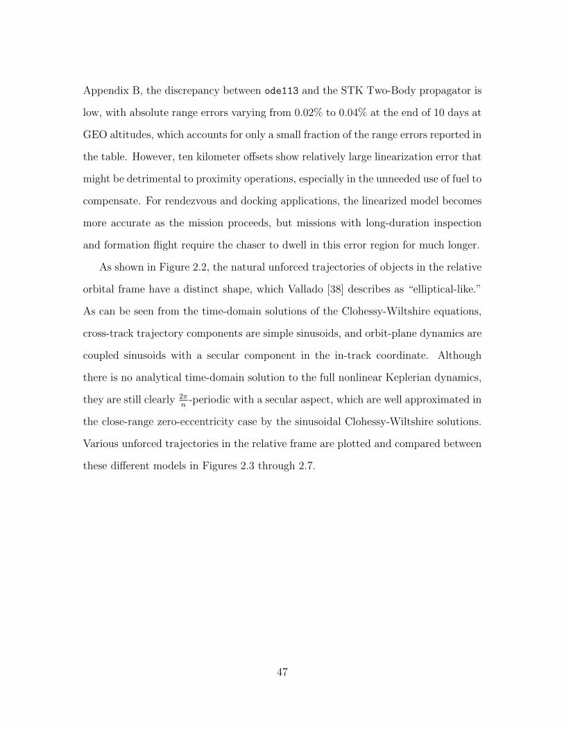
Figure 2.3: Orbital plane trajectories of a GEO object executing various R-bar im-pulses. This causes in-track drift in the Keplerian model, but not under Clohessy-Wiltshire assumptions. Initial radial velocities of 1 m/s, 0.5 m/s, 0.1 m/s, −0.1 m/s,−0.5 m/s, and −1 m/s. (e = 0.0)

In Figure 2.3, it can be seen that an object at rest at the LVLH origin that ex-

ecutes an impulsive burn in the radial direction will set itself on elliptical relative

trajectory which will take a full orbital cycle to return back to the origin. In terms of

classical orbital elements, this impulsive radial burn causes a change in eccentricity

only. Notice that while this behavior is the case for the Clohessy-Wiltshire dynamics,

it is not precisely true in the case of the nonlinear dynamics. It is clear that the Kep-

lerian motion does not return to the original position, but rather ‘behind’ it, notably

for both upward and downward radial burns; this lagging effect can be attributed to

the fact that the radial impulse increased the energy of the chaser’s orbit with respect

to the reference orbit, which is tantamount to increasing semimajor axis (and thus

orbital period) - invalidating the ‘linearizing’ notion that radial burns change only

the orbit’s eccentricity. Mathematical intuition for this behavior can be obtained by

48

examining the vis-viva equation and noticing that increased radial velocity from the

reference orbit, regardless of sign, adds to the orbit’s kinetic energy.

-6

-4

-2

0

2

4

6

Rad

ial (

m)

104

-2.5-2-1.5-1-0.500.511.522.5

In-Track (m) 105

Nonlinear Keplerian MotionClohessy Wiltshire Motion

-2000

-1500

-1000

-500

0

500

2.572.582.592.62.612.62105

-1000

-500

0

500

-2.62-2.61-2.6-2.59-2.58-2.57

105

Actual Orbital Trajectory

Local Horizontal Axis

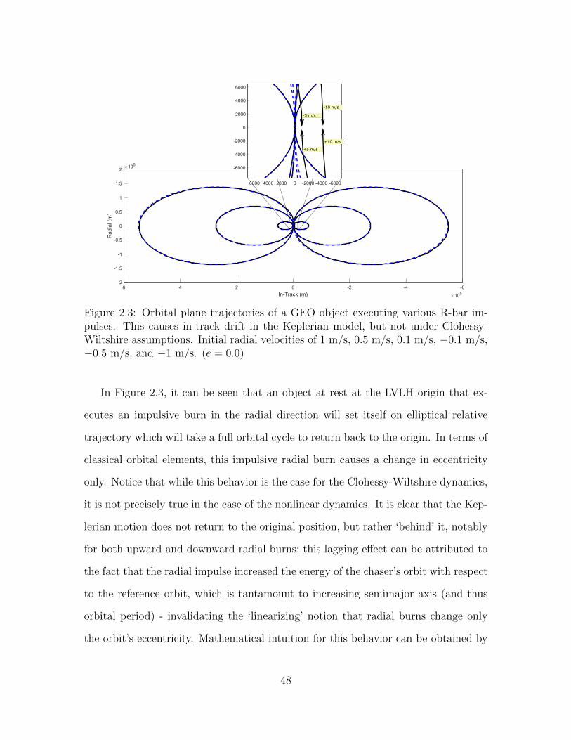
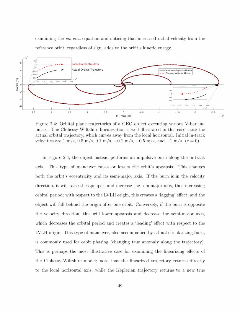
Figure 2.4: Orbital plane trajectories of a GEO object executing various V-bar im-pulses. The Clohessy-Wiltshire linearization is well-illustrated in this case; note theactual orbital trajectory, which curves away from the local horizontal. Initial in-trackvelocities are 1 m/s, 0.5 m/s, 0.1 m/s, −0.1 m/s, −0.5 m/s, and −1 m/s. (e = 0)

In Figure 2.4, the object instead performs an impulsive burn along the in-track

axis. This type of maneuver raises or lowers the orbit’s apoapsis. This changes

both the orbit’s eccentricity and its semi-major axis. If the burn is in the velocity

direction, it will raise the apoapsis and increase the semimajor axis, thus increasing

orbital period; with respect to the LVLH origin, this creates a ‘lagging’ effect, and the

object will fall behind the origin after one orbit. Conversely, if the burn is opposite

the velocity direction, this will lower apoapsis and decrease the semi-major axis,

which decreases the orbital period and creates a ‘leading’ effect with respect to the

LVLH origin. This type of maneuver, also accompanied by a final circularizing burn,

is commonly used for orbit phasing (changing true anomaly along the trajectory).

This is perhaps the most illustrative case for examining the linearizing effects of

the Clohessy-Wiltshire model; note that the linearized trajectory returns directly

to the local horizontal axis, while the Keplerian trajectory returns to a new true

49

anomaly along the orbital trajectory, as is expected. The Clohessy-Wiltshire model’s

linearization can be thought of as extending the target’s orbital trajectory into a

straight line along the local horizontal, while holding its velocity’s magnitude and

direction constant along the axis. Clearly, this assumption only holds at very close

proximity and on short time scales.

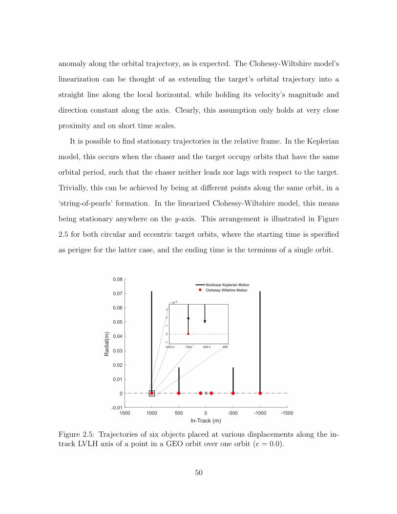
It is possible to find stationary trajectories in the relative frame. In the Keplerian

model, this occurs when the chaser and the target occupy orbits that have the same

orbital period, such that the chaser neither leads nor lags with respect to the target.

Trivially, this can be achieved by being at different points along the same orbit, in a

‘string-of-pearls’ formation. In the linearized Clohessy-Wiltshire model, this means

being stationary anywhere on the y-axis. This arrangement is illustrated in Figure

2.5 for both circular and eccentric target orbits, where the starting time is specified

as perigee for the latter case, and the ending time is the terminus of a single orbit.

-0.01

0

0.01

0.02

0.03

0.04

0.05

0.06

0.07

0.08

Rad

ial(m

)

-1500-1000-500050010001500

In-Track (m)

-1

0

1

2

3

10-5

999999.510001000.5

Nonlinear Keplerian Motion

Clohessy Wiltshire Motion

Figure 2.5: Trajectories of six objects placed at various displacements along the in-track LVLH axis of a point in a GEO orbit over one orbit (e = 0.0).

50

As would be expected by substituting zero-velocity and zero-radial-offset initial

conditions into the Clohessy-Wiltshire equations, the linear model predicts no motion.

The nonlinear model predicts a small amount of oscillatory behavior of centimeter-

scale amplitude. This can be understood by realizing that the target’s orbital tra-

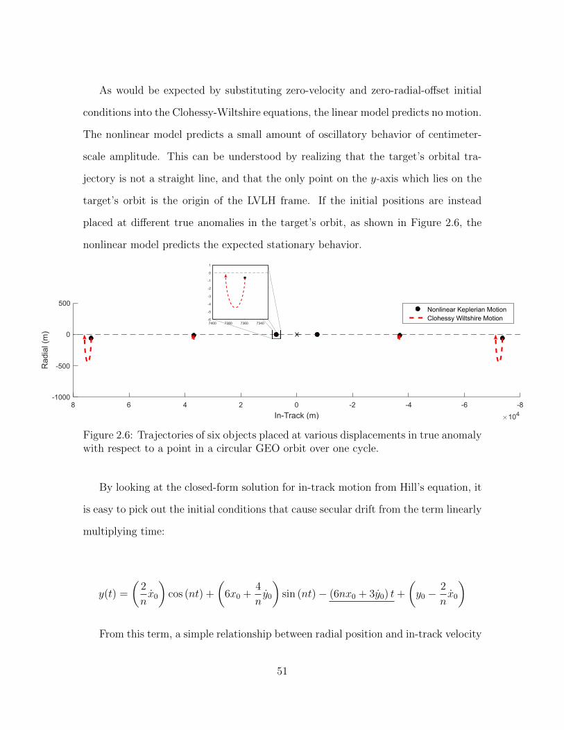
jectory is not a straight line, and that the only point on the y-axis which lies on the

target’s orbit is the origin of the LVLH frame. If the initial positions are instead

placed at different true anomalies in the target’s orbit, as shown in Figure 2.6, the

nonlinear model predicts the expected stationary behavior.

-1000

-500

0

500

Rad

ial (

m)

-8-6-4-202468

In-Track (m) 104

Nonlinear Keplerian MotionClohessy Wiltshire Motion-6

-5

-4

-3

-2

-1

0

1

7340736073807400

Figure 2.6: Trajectories of six objects placed at various displacements in true anomalywith respect to a point in a circular GEO orbit over one cycle.

By looking at the closed-form solution for in-track motion from Hill’s equation, it

is easy to pick out the initial conditions that cause secular drift from the term linearly

multiplying time:

y(t) =

(2

nx0

)cos (nt) +

(6x0 +

4

ny0

)sin (nt)− (6nx0 + 3y0) t+

(y0 −

2

nx0

)

From this term, a simple relationship between radial position and in-track velocity

51

can be obtained which nulls the secular drifting of relative motion in the linear model:

y0 = −2nx0

In the previous case, where the chaser was able to remain stationary along the Y -

axis in the Clohessy-Wiltshire model, this condition was trivially met (both y0 and x0

were zero); the chaser was following the trajectory of a degenerate ellipse with semi-

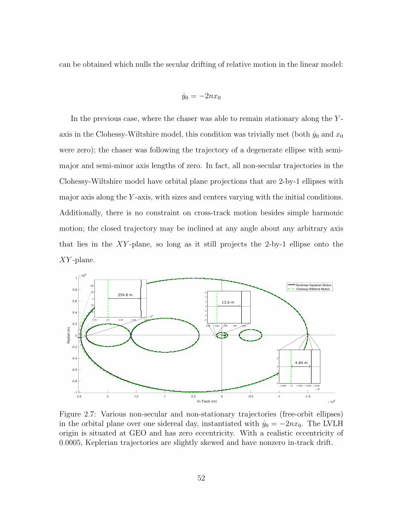
major and semi-minor axis lengths of zero. In fact, all non-secular trajectories in the

Clohessy-Wiltshire model have orbital plane projections that are 2-by-1 ellipses with

major axis along the Y -axis, with sizes and centers varying with the initial conditions.

Additionally, there is no constraint on cross-track motion besides simple harmonic

motion; the closed trajectory may be inclined at any angle about any arbitrary axis

that lies in the XY -plane, so long as it still projects the 2-by-1 ellipse onto the

XY -plane.

-1

-0.8

-0.6

-0.4

-0.2

0

0.2

0.4

0.6

0.8

1

Rad

ial (

m)

104

-1.5-1-0.500.511.522.5

In-Track (m) 104

Nonlinear Keplerian MotionClohessy-Wiltshire Motion

-100

-50

0

50

100

2.472.482.492.52.51

104

254.8 m

-6

-4

-2

0

2

4

6

98599099510001005

13.6 m

-4

-2

0

2

4

-1.5006-1.5004-1.5002-1.5-1.4998

104

4.84 m

Figure 2.7: Various non-secular and non-stationary trajectories (free-orbit ellipses)in the orbital plane over one sidereal day, instantiated with y0 = −2nx0. The LVLHorigin is situated at GEO and has zero eccentricity. With a realistic eccentricity of0.0005, Keplerian trajectories are slightly skewed and have nonzero in-track drift.

52

This trajectory, shown in Figure 2.7, is referred to by a number of names such as

the ‘free-orbit ellipse,’ ‘safety ellipse,’ ‘inspection ellipse,’ or ‘circumnavigation ellipse.’

It is of great interest in the field of proximity operations because it is an unforced

trajectory that allows periodic motion about a fixed point in the LVLH frame under

the Clohessy-Wiltshire assumptions.

This shape of relative motion trajectory arises when the chaser’s orbit has pre-

cisely the same period as the target’s orbit, but has a lower periapsis and a higher

apoapsis than the target’s orbit. In terms of the classical elements, this means that

both orbits have the same semimajor axis a, but the chaser’s orbit has slightly more

eccentricity, δe. There may also be a difference in inclination, δi, which manifests

itself as harmonic out-of-plane motion; a difference in the argument of perigee, δω,

shifts the center of the ellipse along the in-track axis (equivalently, this can be ob-

tained by a different true anomaly on the same orbit). It is thus intuitively clear

that closed periodic relative trajectories do still exist under the nonlinear Keplerian

model (which assumes only Two-Body forces), but with shapes that are not perfect

ellipses; instead, the nonlinearity of the eccentricity differential results in distorted,

‘bean-shaped’ trajectories, which becomes more prominent with more eccentric target

orbits.

53

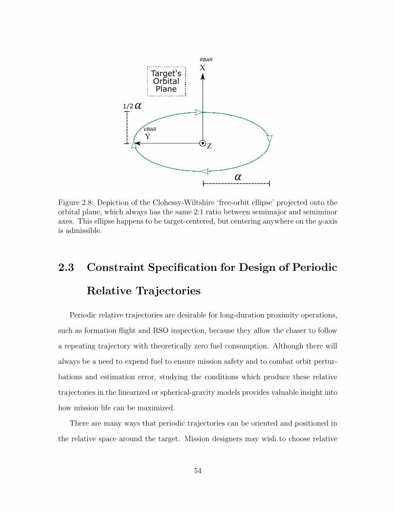
Target's OrbitalPlane

X

Z

RBAR

1/2

YVBAR

𝛼

𝛼

Figure 2.8: Depiction of the Clohessy-Wiltshire ‘free-orbit ellipse’ projected onto theorbital plane, which always has the same 2:1 ratio between semimajor and semiminoraxes. This ellipse happens to be target-centered, but centering anywhere on the y-axisis admissible.

2.3 Constraint Specification for Design of Periodic

Relative Trajectories

Periodic relative trajectories are desirable for long-duration proximity operations,

such as formation flight and RSO inspection, because they allow the chaser to follow

a repeating trajectory with theoretically zero fuel consumption. Although there will

always be a need to expend fuel to ensure mission safety and to combat orbit pertur-

bations and estimation error, studying the conditions which produce these relative

trajectories in the linearized or spherical-gravity models provides valuable insight into

how mission life can be maximized.

There are many ways that periodic trajectories can be oriented and positioned in

the relative space around the target. Mission designers may wish to choose relative

54

trajectories that suit their users’ needs; for example, the relative trajectory can be

designed to periodically pass within the field of view of certain sensors on the target,

or to avoid them. It may be desirable to specify a minimum range (e.g., based on

safety requirements) or maximum range (e.g., based on sensor requirements) to the

target, either in a circumnavigating trajectory or one that is offset in true anomaly.

An example of a purposefully-designed relative trajectory is described by Naasz

[29]: If the trajectory has zero in-track offset, and equal range maxima in the radial

and cross-track directions, the chaser-to-target direction in inertial space varies by no

more than about 30 degrees from some mean inertial direction in the target’s orbital

plane (e.g., the Earth-Sun vector), which is useful for power and lighting considera-

tions. As another example, a trajectory with a 60°-inclined relative trajectory about

the in-track axis maintains constant range with the target to first-order linearization,

which may be useful in some circumstances for sensor calibration or inspection.

In this section, periodic trajectory design is posed as a set of constraints on the

LVLH coordinates for both the linearized and full Keplerian models. The process is

straightforward for the linearized model due to the geometrical simplicity of the free-

orbit ellipse and the availability of closed-form sinusoidal solutions to the equations

of motion. It is more difficult for the nonlinear model; here, a differential-orbital-

element approach expressed in the LVLH variables is used. The ultimate goal is to be

able to express a set of path constraints on the relative state variables that produces

this desirable relative motion, which proves useful for eventual implementation in the

numerical trajectory optimization framework.

55

2.3.1 Specifying the Clohessy-Wiltshire Free-Orbit Ellipse

The linear free-orbit ellipse can be entirely specified by five equality constraints on

the LVLH state variables, essentially derivable from the geometry of a standard ellipse.

The first and most essential constraint is the non-secularity constraint introduced

above. This ensures a closed trajectory with the characteristic 2-by-1 elliptical shape.

To specify the size and center of the ellipse using the LVLH state variables, it is

helpful to leverage the general equation of an ellipse in cartesian coordinates:

x2

β2+

(y − yc)2α2

= 1

Where α is the semimajor axis of the ellipse, β is the semiminor axis, and yc is

the displacement of the ellipse’s center along the y-axis. In the case of the free-

orbit ellipse’s projection onto the orbital plane, the ratio between α and β is always

constant. Thus, it is possible multiply through by α to obtain:

4x2 + (y − yc)2 = α2

Although this equation includes both yc and α, it only constrains the x and y position

coordinates. In some applications, it may also be necessary to develop a relationship

that also constrains the velocities of the in-plane coordinates. To obtain such a

relation, one can implicitly differentiate the ellipse equation with respect to one of

the coordinates:

56

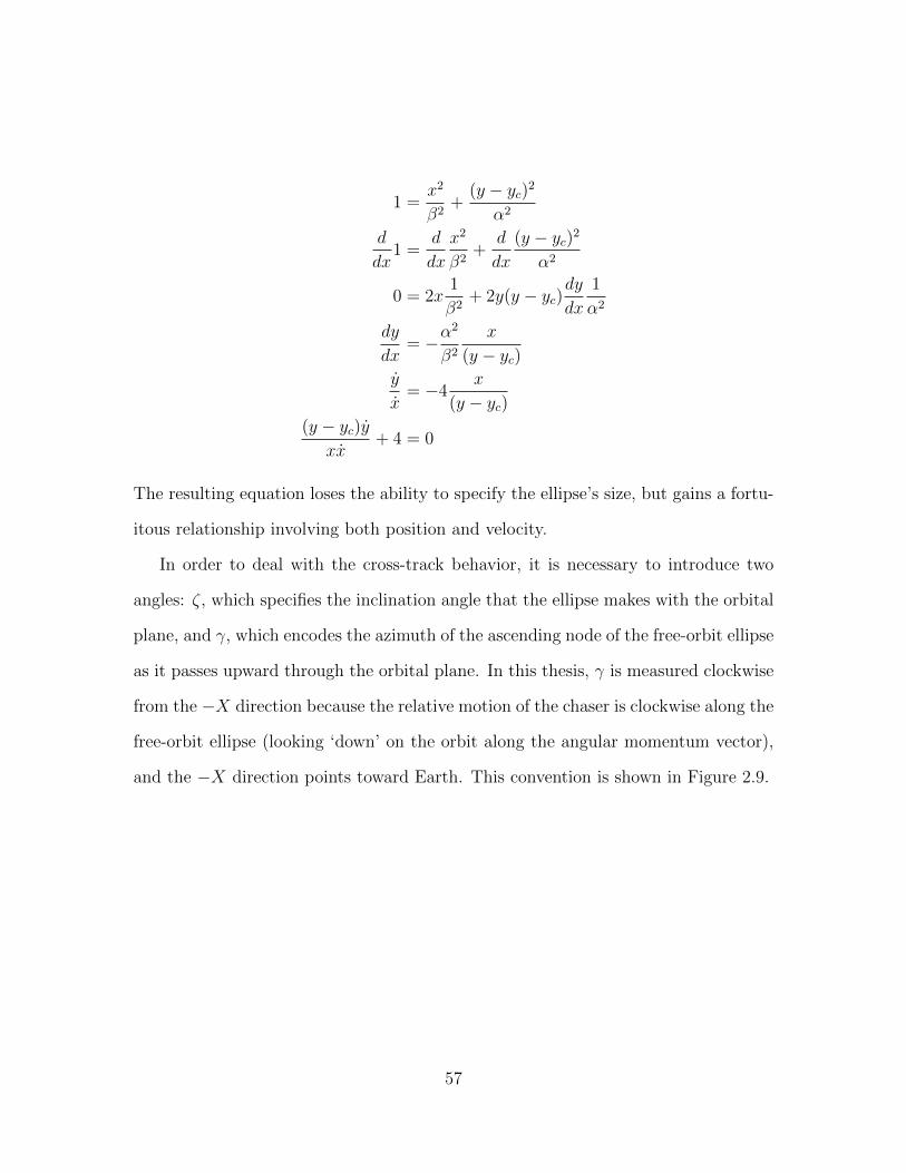
1 =x2

β2+

(y − yc)2α2

d

dx1 =

d

dx

x2

β2+

d

dx

(y − yc)2α2

0 = 2x1

β2+ 2y(y − yc)

dy

dx

1

α2

dy

dx= −α

2

β2

x

(y − yc)y

x= −4

x

(y − yc)(y − yc)y

xx+ 4 = 0

The resulting equation loses the ability to specify the ellipse’s size, but gains a fortu-

itous relationship involving both position and velocity.

In order to deal with the cross-track behavior, it is necessary to introduce two

angles: ζ, which specifies the inclination angle that the ellipse makes with the orbital

plane, and γ, which encodes the azimuth of the ascending node of the free-orbit ellipse

as it passes upward through the orbital plane. In this thesis, γ is measured clockwise

from the −X direction because the relative motion of the chaser is clockwise along the

free-orbit ellipse (looking ‘down’ on the orbit along the angular momentum vector),

and the −X direction points toward Earth. This convention is shown in Figure 2.9.

57

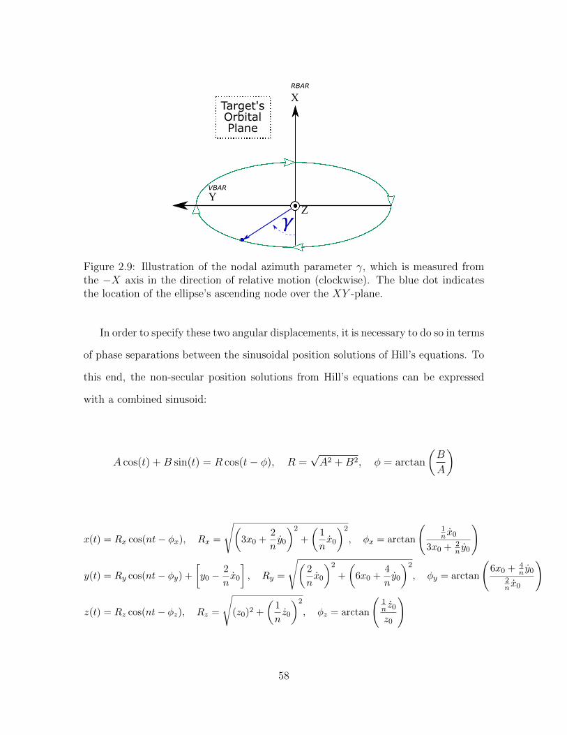
Target's OrbitalPlane

X

Z

RBAR

𝛾

YVBAR

Figure 2.9: Illustration of the nodal azimuth parameter γ, which is measured fromthe −X axis in the direction of relative motion (clockwise). The blue dot indicatesthe location of the ellipse’s ascending node over the XY -plane.

In order to specify these two angular displacements, it is necessary to do so in terms

of phase separations between the sinusoidal position solutions of Hill’s equations. To

this end, the non-secular position solutions from Hill’s equations can be expressed

with a combined sinusoid:

A cos(t) +B sin(t) = R cos(t− φ), R =√A2 +B2, φ = arctan

(B

A

)

x(t) = Rx cos(nt− φx), Rx =

√(3x0 +

2

ny0

)2

+

(1

nx0

)2

, φx = arctan

(1n x0

3x0 +2n y0

)

y(t) = Ry cos(nt− φy) +[y0 −

2

nx0

], Ry =

√(2

nx0

)2

+

(6x0 +

4

ny0

)2

, φy = arctan

(6x0 +

4n y0

2n x0

)

z(t) = Rz cos(nt− φz), Rz =

√(z0)2 +

(1

nz0

)2

, φz = arctan

(1n z0

z0

)

58

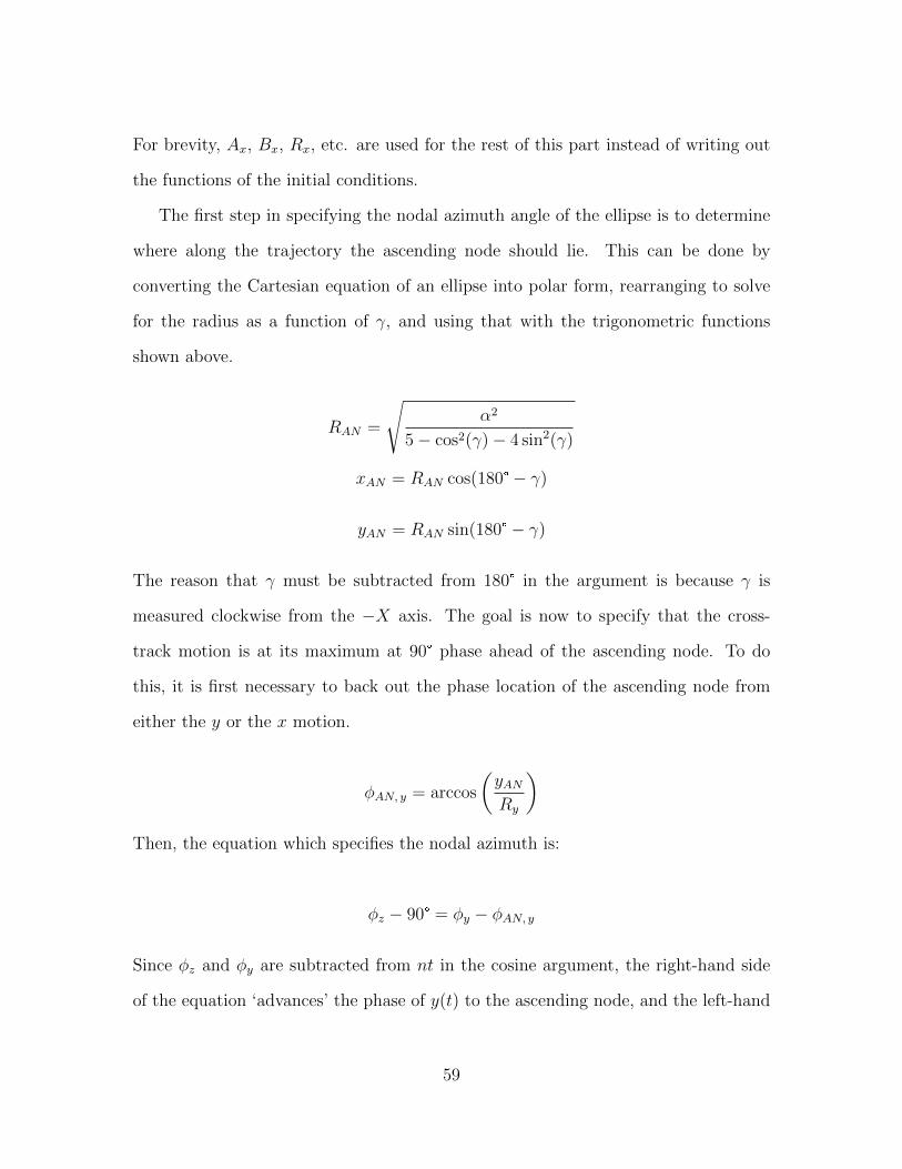
For brevity, Ax, Bx, Rx, etc. are used for the rest of this part instead of writing out

the functions of the initial conditions.

The first step in specifying the nodal azimuth angle of the ellipse is to determine

where along the trajectory the ascending node should lie. This can be done by

converting the Cartesian equation of an ellipse into polar form, rearranging to solve

for the radius as a function of γ, and using that with the trigonometric functions

shown above.

RAN =

√α2

5− cos2(γ)− 4 sin2(γ)

xAN = RAN cos(180°− γ)

yAN = RAN sin(180°− γ)

The reason that γ must be subtracted from 180° in the argument is because γ is

measured clockwise from the −X axis. The goal is now to specify that the cross-

track motion is at its maximum at 90° phase ahead of the ascending node. To do

this, it is first necessary to back out the phase location of the ascending node from

either the y or the x motion.

φAN, y = arccos

(yANRy

)Then, the equation which specifies the nodal azimuth is:

φz − 90° = φy − φAN, y

Since φz and φy are subtracted from nt in the cosine argument, the right-hand side

of the equation ‘advances’ the phase of y(t) to the ascending node, and the left-hand

59

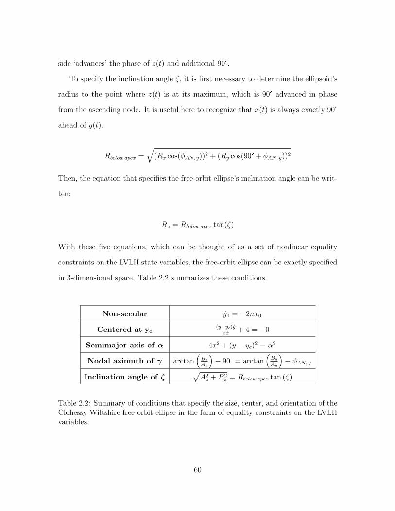
side ‘advances’ the phase of z(t) and additional 90°.

To specify the inclination angle ζ, it is first necessary to determine the ellipsoid’s

radius to the point where z(t) is at its maximum, which is 90° advanced in phase

from the ascending node. It is useful here to recognize that x(t) is always exactly 90°

ahead of y(t).

Rbelow apex =√

(Rx cos(φAN, y))2 + (Ry cos(90° + φAN, y))2

Then, the equation that specifies the free-orbit ellipse’s inclination angle can be writ-

ten:

Rz = Rbelow apex tan(ζ)

With these five equations, which can be thought of as a set of nonlinear equality

constraints on the LVLH state variables, the free-orbit ellipse can be exactly specified

in 3-dimensional space. Table 2.2 summarizes these conditions.

Non-secular y0 = −2nx0

Centered at yc(y−yc)yxx

+ 4 = −0

Semimajor axis of α 4x2 + (y − yc)2 = α2

Nodal azimuth of γ arctan(Bz

Az

)− 90° = arctan

(By

Ay

)− φAN, y

Inclination angle of ζ√A2z +B2

z = Rbelow apex tan (ζ)

Table 2.2: Summary of conditions that specify the size, center, and orientation of theClohessy-Wiltshire free-orbit ellipse in the form of equality constraints on the LVLHvariables.

60

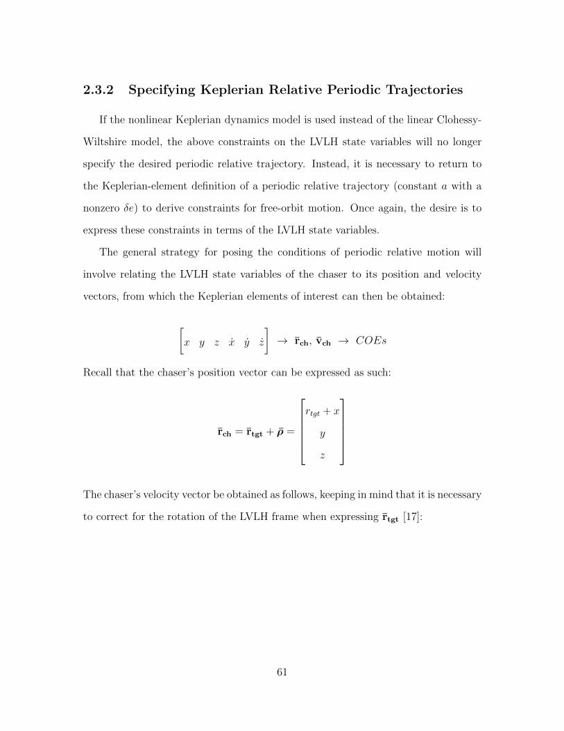
2.3.2 Specifying Keplerian Relative Periodic Trajectories

If the nonlinear Keplerian dynamics model is used instead of the linear Clohessy-

Wiltshire model, the above constraints on the LVLH state variables will no longer

specify the desired periodic relative trajectory. Instead, it is necessary to return to

the Keplerian-element definition of a periodic relative trajectory (constant a with a

nonzero δe) to derive constraints for free-orbit motion. Once again, the desire is to

express these constraints in terms of the LVLH state variables.

The general strategy for posing the conditions of periodic relative motion will

involve relating the LVLH state variables of the chaser to its position and velocity

vectors, from which the Keplerian elements of interest can then be obtained:

[x y z x y z

]→ rch, vch → COEs

Recall that the chaser’s position vector can be expressed as such:

rch = rtgt + ρ =

rtgt + x

y

z

The chaser’s velocity vector be obtained as follows, keeping in mind that it is necessary

to correct for the rotation of the LVLH frame when expressing rtgt [17]:

61

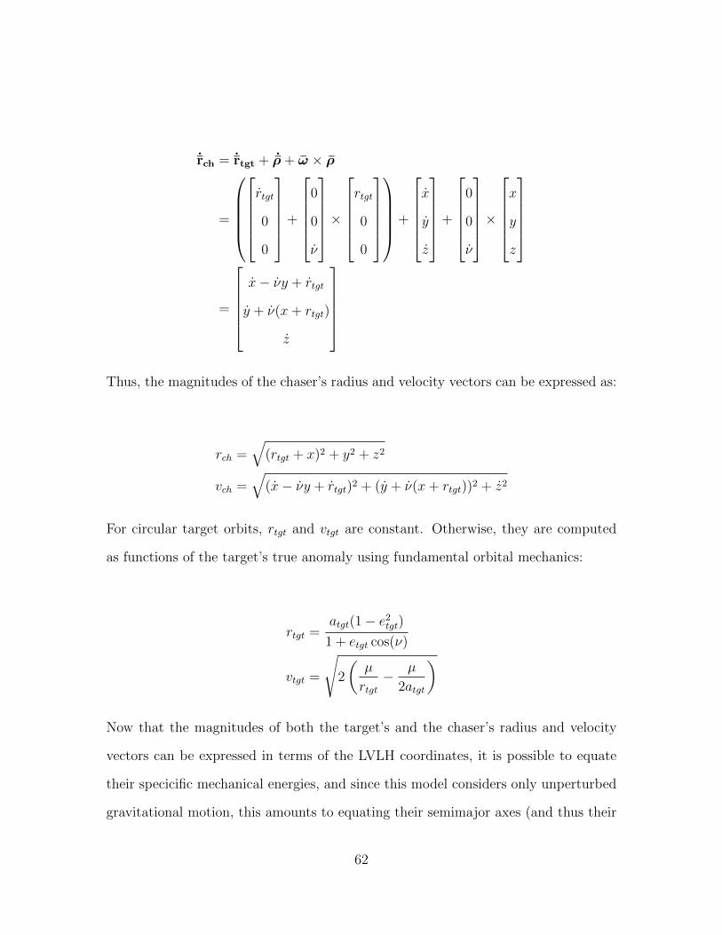
˙rch = ˙rtgt + ˙ρ+ ω × ρ

=

rtgt

0

0

+

0

0

ν

×rtgt

0

0

+

x

y

z

+

0

0

ν

×x

y

z

=

x− νy + rtgt

y + ν(x+ rtgt)

z

Thus, the magnitudes of the chaser’s radius and velocity vectors can be expressed as:

rch =√

(rtgt + x)2 + y2 + z2

vch =√

(x− νy + rtgt)2 + (y + ν(x+ rtgt))2 + z2

For circular target orbits, rtgt and vtgt are constant. Otherwise, they are computed

as functions of the target’s true anomaly using fundamental orbital mechanics:

rtgt =atgt(1− e2tgt)

1 + etgt cos(ν)

vtgt =

√2

(µ

rtgt− µ

2atgt

)

Now that the magnitudes of both the target’s and the chaser’s radius and velocity

vectors can be expressed in terms of the LVLH coordinates, it is possible to equate

their specicific mechanical energies, and since this model considers only unperturbed

gravitational motion, this amounts to equating their semimajor axes (and thus their

62

orbital periods). This results in a periodic free-orbit relative trajectory for the chaser.

Manipulation of the vis-viva equation allows this energy-matching constraint to be

written:

Ttgt = Tch ∴ atgt = ach ∴ ξtgt = ξch

v2tgt2− µ

rtgt=

v2ch2− µ

rch

− µ

2atgt=

v2ch2− µ

rch

Satisfaction of the energy-matching constraint guarantees periodic motion, but it

may also be desirable to have some way to specify size and the in-track offset of

the trajectory. For these two parameters, it is necessary to compute the eccentricity

vectors and magnitudes for both objects, if they exist. The size of the relative orbit

is related to the differential eccentricity, while the offset of the relative orbit is related

to the angle between the eccentricity vectors (a differential argument of perigee).

etgt =1

µ

(v2tgt −

µ

rtgt

)rtgt

0

0

−rtgt

0

0

·rtgt

νrtgt

0

rtgt

νrtgt

0

=1

µ

ν2r3tgt − µ

−νrtgtr2tgt0

etgt = |etgt|

63

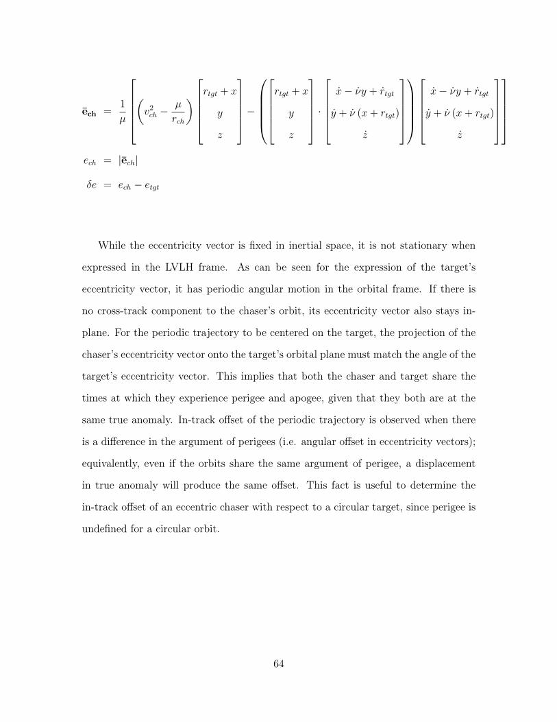
ech =1

µ

(v2ch −

µ

rch

)rtgt + x

y

z

−rtgt + x

y

z

·x− νy + rtgt

y + ν (x+ rtgt)

z

x− νy + rtgt

y + ν (x+ rtgt)

z

ech = |ech|

δe = ech − etgt

While the eccentricity vector is fixed in inertial space, it is not stationary when

expressed in the LVLH frame. As can be seen for the expression of the target’s

eccentricity vector, it has periodic angular motion in the orbital frame. If there is

no cross-track component to the chaser’s orbit, its eccentricity vector also stays in-

plane. For the periodic trajectory to be centered on the target, the projection of the

chaser’s eccentricity vector onto the target’s orbital plane must match the angle of the

target’s eccentricity vector. This implies that both the chaser and target share the

times at which they experience perigee and apogee, given that they both are at the

same true anomaly. In-track offset of the periodic trajectory is observed when there

is a difference in the argument of perigees (i.e. angular offset in eccentricity vectors);

equivalently, even if the orbits share the same argument of perigee, a displacement

in true anomaly will produce the same offset. This fact is useful to determine the

in-track offset of an eccentric chaser with respect to a circular target, since perigee is

undefined for a circular orbit.

64

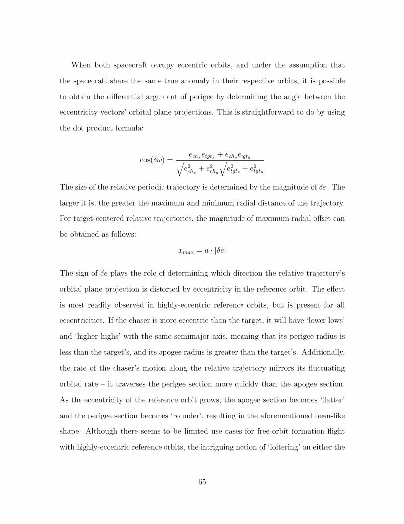
When both spacecraft occupy eccentric orbits, and under the assumption that

the spacecraft share the same true anomaly in their respective orbits, it is possible

to obtain the differential argument of perigee by determining the angle between the

eccentricity vectors’ orbital plane projections. This is straightforward to do by using

the dot product formula:

cos(δω) =echxetgtx + echyetgty√e2chx + e2chy

√e2tgtx + e2tgty

The size of the relative periodic trajectory is determined by the magnitude of δe. The

larger it is, the greater the maximum and minimum radial distance of the trajectory.

For target-centered relative trajectories, the magnitude of maximum radial offset can

be obtained as follows:

xmax = a · |δe|

The sign of δe plays the role of determining which direction the relative trajectory’s

orbital plane projection is distorted by eccentricity in the reference orbit. The effect

is most readily observed in highly-eccentric reference orbits, but is present for all

eccentricities. If the chaser is more eccentric than the target, it will have ‘lower lows’

and ‘higher highs’ with the same semimajor axis, meaning that its perigee radius is

less than the target’s, and its apogee radius is greater than the target’s. Additionally,

the rate of the chaser’s motion along the relative trajectory mirrors its fluctuating

orbital rate – it traverses the perigee section more quickly than the apogee section.

As the eccentricity of the reference orbit grows, the apogee section becomes ‘flatter’

and the perigee section becomes ‘rounder’, resulting in the aforementioned bean-like

shape. Although there seems to be limited use cases for free-orbit formation flight

with highly-eccentric reference orbits, the intriguing notion of ‘loitering’ on either the

65

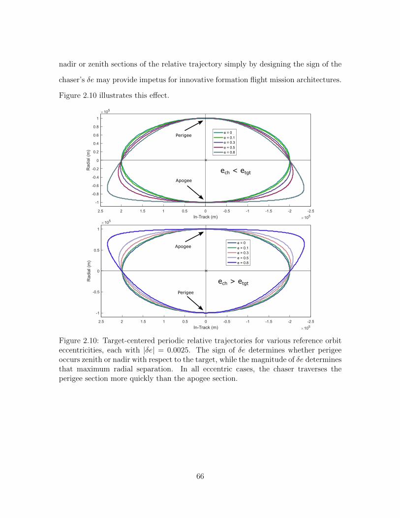
nadir or zenith sections of the relative trajectory simply by designing the sign of the

chaser’s δe may provide impetus for innovative formation flight mission architectures.

Figure 2.10 illustrates this effect.

-1

-0.5

0

0.5

1

Rad

ial (

m)

105

-2.5-2-1.5-1-0.500.511.522.5

In-Track (m) 105

e = 0

e = 0.1e = 0.3

e = 0.5e = 0.8

-1

-0.8

-0.6

-0.4

-0.2

0

0.2

0.4

0.6

0.8

1

Rad

ial (

m)

105

-2.5-2-1.5-1-0.500.511.522.5

In-Track (m) 105

e = 0

e = 0.1e = 0.3

e = 0.5e = 0.8

ech < etgt

ech > etgt

Apogee

Apogee

Perigee

Perigee

Figure 2.10: Target-centered periodic relative trajectories for various reference orbiteccentricities, each with |δe| = 0.0025. The sign of δe determines whether perigeeoccurs zenith or nadir with respect to the target, while the magnitude of δe determinesthat maximum radial separation. In all eccentric cases, the chaser traverses theperigee section more quickly than the apogee section.

66

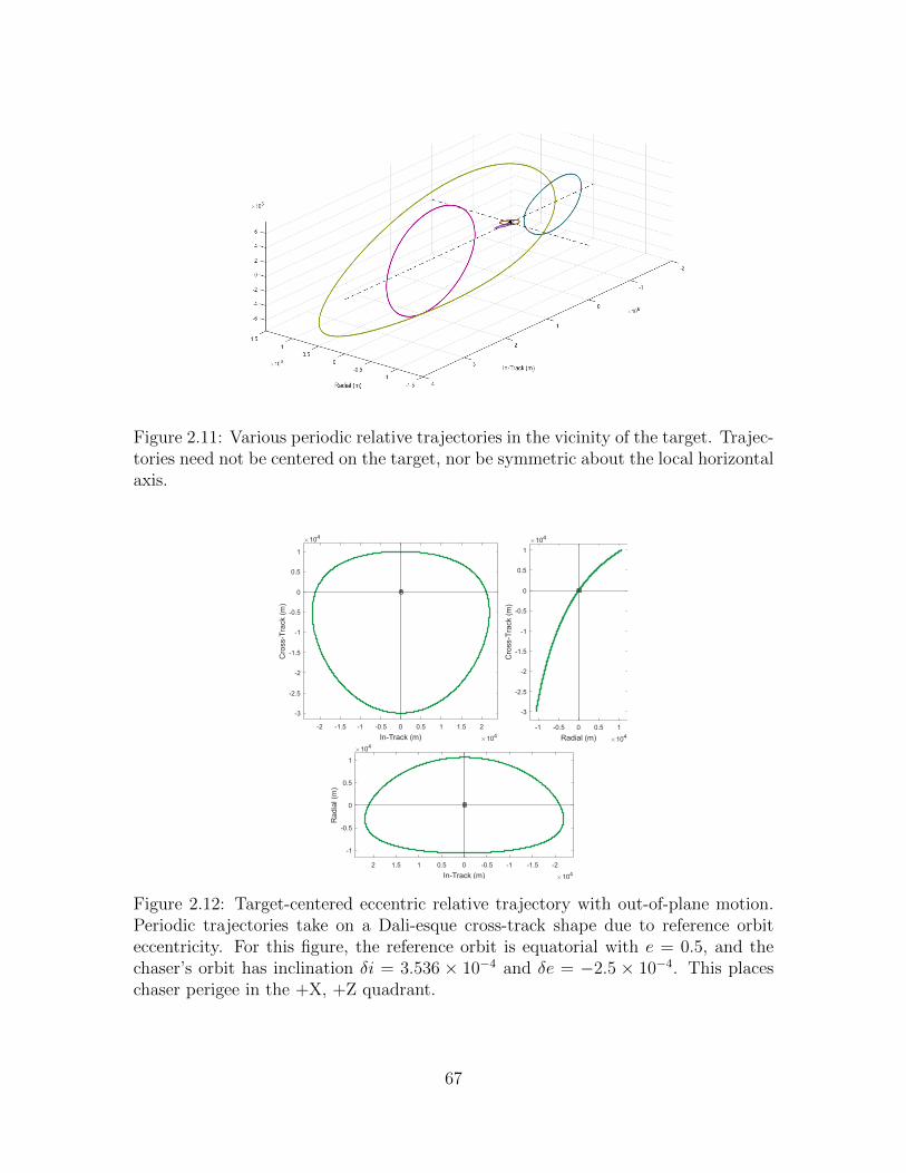
Figure 2.11: Various periodic relative trajectories in the vicinity of the target. Trajec-tories need not be centered on the target, nor be symmetric about the local horizontalaxis.

-2 -1.5 -1 -0.5 0 0.5 1 1.5 2

In-Track (m) 104

-3

-2.5

-2

-1.5

-1

-0.5

0

0.5

1

Cro

ss-T

rack

(m

)

104

-1

-0.5

0

0.5

1

Rad

ial (

m)

104

-2-1.5-1-0.500.511.52

In-Track (m) 104

-1 -0.5 0 0.5 1

Radial (m) 104

-3

-2.5

-2

-1.5

-1

-0.5

0

0.5

1

Cro

ss-T

rack

(m

)

104

Figure 2.12: Target-centered eccentric relative trajectory with out-of-plane motion.Periodic trajectories take on a Dali-esque cross-track shape due to reference orbiteccentricity. For this figure, the reference orbit is equatorial with e = 0.5, and thechaser’s orbit has inclination δi = 3.536 × 10−4 and δe = −2.5 × 10−4. This placeschaser perigee in the +X, +Z quadrant.

67

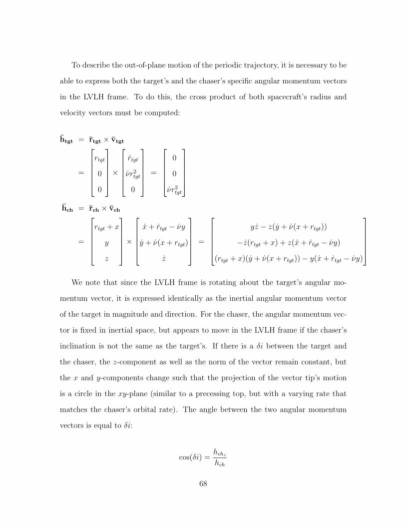
To describe the out-of-plane motion of the periodic trajectory, it is necessary to be

able to express both the target’s and the chaser’s specific angular momentum vectors

in the LVLH frame. To do this, the cross product of both spacecraft’s radius and

velocity vectors must be computed:

htgt = rtgt × vtgt

=

rtgt

0

0

×rtgt

νr2tgt

0

=

0

0

νr2tgt

hch = rch × vch

=

rtgt + x

y

z

×x+ rtgt − νy

y + ν(x+ rtgt)

z

=

yz − z(y + ν(x+ rtgt))

−z(rtgt + x) + z(x+ rtgt − νy)

(rtgt + x)(y + ν(x+ rtgt))− y(x+ rtgt − νy)

We note that since the LVLH frame is rotating about the target’s angular mo-

mentum vector, it is expressed identically as the inertial angular momentum vector

of the target in magnitude and direction. For the chaser, the angular momentum vec-

tor is fixed in inertial space, but appears to move in the LVLH frame if the chaser’s

inclination is not the same as the target’s. If there is a δi between the target and

the chaser, the z-component as well as the norm of the vector remain constant, but

the x and y-components change such that the projection of the vector tip’s motion

is a circle in the xy-plane (similar to a precessing top, but with a varying rate that

matches the chaser’s orbital rate). The angle between the two angular momentum

vectors is equal to δi:

cos(δi) =hchzhch

68

Obtaining the azimuth of the local ascending node in the LVLH frame is more

involved than the simple vector operations employed to obtain δe, δi, and δω. For

this reason, the following analysis is restricted to target-centered trajectories with an

equatorial reference orbit. In this simplified case, the eccentricity vector projections

of the target and the chaser are always parallel in the orbital plane, and thus the

differential eccentricity vector δe = etgt − ech always points from the LVLH origin

to the chaser’s position along the relative trajectory. The vector that points to the

location where the chaser’s orbit ‘ascends’ through the target orbital plane can be

obtained as the cross product of their specific angular momentum vectors:

Nrel = htgt × hch

Since both this local ascending node vector and the differential eccentricity vector are

considered to be fixed in inertial space, their angular offset in the LVLH orbital plane

remains constant throughout the orbit. In essence, the azimuth of the local ascending

node can be designed by correctly instantiating the chaser’s angular momentum vector

with respect to the chaser’s eccentricity vector. It is important to also keep in mind

that the sign of δe changes where in the LVLH frame the chaser experiences perigee.

Let the parameter Γ represent the angular separation between the chaser’s relative

ascending node and the shared perigee. Then,

cos Γ =Nrelxδex +Nrelyδey√N2relx

+N2rely

√δe2x + δe2y

69

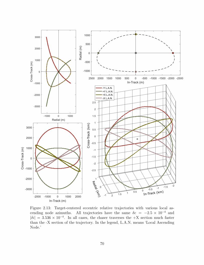
-1

0

1

-2-1.5-1-0.500.511.52

-2.5

-2

-1.5

-1

-0.5

0

0.5

1

1.5

2

2.5

In-Track (km)

Radial (km

)

Cro

ss-T

rack

(km

)-Y L.A.N.

+Y L.A.N.+X L.A.N.

-X L.A.N.

-1000 0 1000

Radial (m)

-3000

-2000

-1000

0

1000

2000

3000

Cro

ss-T

rack

(m

)

-2000 -1000 0 1000 2000

In-Track (m)

-3000

-2000

-1000

0

1000

2000

3000

Cro

ss-T

rack

(m

)

-1000

-500

0

500

1000

Rad

ial (

m)

-2500-2000-1500-1000-50005001000150020002500

In-Track (m)

Figure 2.13: Target-centered eccentric relative trajectories with various local as-cending node azimuths. All trajectories have the same δe = −2.5 × 10−4 and|δi| = 3.536 × 10−4. In all cases, the chaser traverses the +X section much fasterthan the -X section of the trajectory. In the legend, L.A.N. means ‘Local AscendingNode.’

70

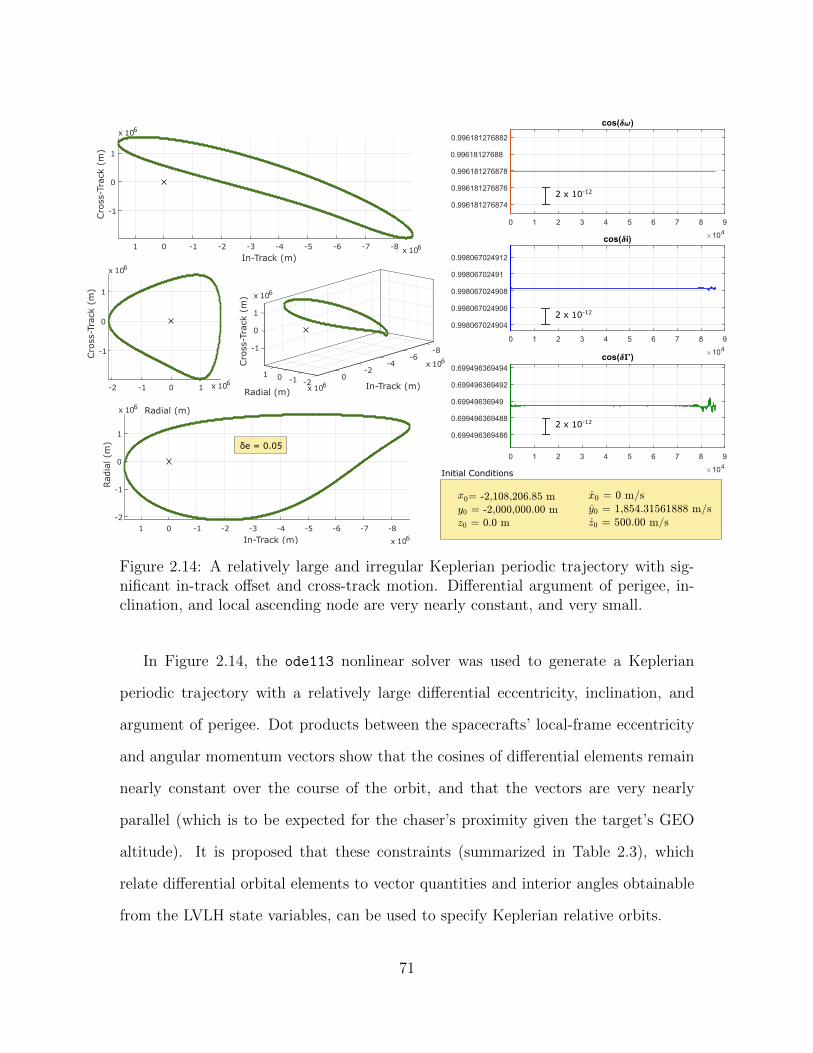
-8-7-6-5-4-3-2-101

In-Track (m)x 106

-1

0

1

Cro

ss-T

rack

(m

)

x 106

-2

-1

0

1

Rad

ial (m

)

x 106

-8-7-6-5-4-3-2-101

In-Track (m) x 106

-2 -1 0 1

Radial (m)

x 106

-1

0

1

Cro

ss-T

rack

(m

)

x 106

-8-6

-4

In-Track (m)

x 106-2

-1

0

Cro

ss-T

rack

(m

) x 106

1

1

Radial (m) x 10600 -1 -2

Initial Conditions

2 x 10-12

2 x 10-12

2 x 10-12

δe = 0.05

Figure 2.14: A relatively large and irregular Keplerian periodic trajectory with sig-nificant in-track offset and cross-track motion. Differential argument of perigee, in-clination, and local ascending node are very nearly constant, and very small.

In Figure 2.14, the ode113 nonlinear solver was used to generate a Keplerian

periodic trajectory with a relatively large differential eccentricity, inclination, and

argument of perigee. Dot products between the spacecrafts’ local-frame eccentricity

and angular momentum vectors show that the cosines of differential elements remain

nearly constant over the course of the orbit, and that the vectors are very nearly

parallel (which is to be expected for the chaser’s proximity given the target’s GEO

altitude). It is proposed that these constraints (summarized in Table 2.3), which

relate differential orbital elements to vector quantities and interior angles obtainable

from the LVLH state variables, can be used to specify Keplerian relative orbits.

71

Non-secular − µ2a

=v2ch2− µ

rch

In-track offset of δω cos(δω) =echxetgtx+echy etgty√e2chx+e

2chy

√e2tgtx+e

2tgty

Radial size of xmax (target-centered) xmax = a · |δe|

Inclination angle of δi cos(δi) =hchzhch

Relative nodal azimuth of Γ cos Γ =Nrelxδex+Nrely δey√N2

relx+N2

rely

√δe2x+δe

2y

Target radius in LVLH frame rtgt = [rtgt 0 0]T

Target velocity in LVLH frame vtgt =[rtgt νr2tgt 0

]TChaser radius in LVLH frame rch = [rtgt + x y z]T

Chaser velocity in LVLH frame vch = [rtgt + x− νy y + ν(rtgt + x) z]T

Table 2.3: Summary of proposed equality constraints to specify Keplerian relativeperiodic trajectories.

Due to the sizable effect of extremely small variations in orbital elements on rel-

ative trajectories, it may not be practically feasible to obtain precise enough mea-

surements of relative position and velocity to accurately compute constraint values

in a real application. At close ranges where high-fidelity measurements may be ob-

tainable, the periodic trajectory is extremely sensitive to variations in differential

Keplerian elements; at long ranges, the trajectory might involve less minuscule vari-

ations, but obtaining a precise relative measurement is more difficult. Possibly due

in part to this ‘macro/micro’ scaling conundrum, the trajectory optimization soft-

ware introduced in Chapter 3 was unsuccessful in satisfactorily implementing these

constraints.

72

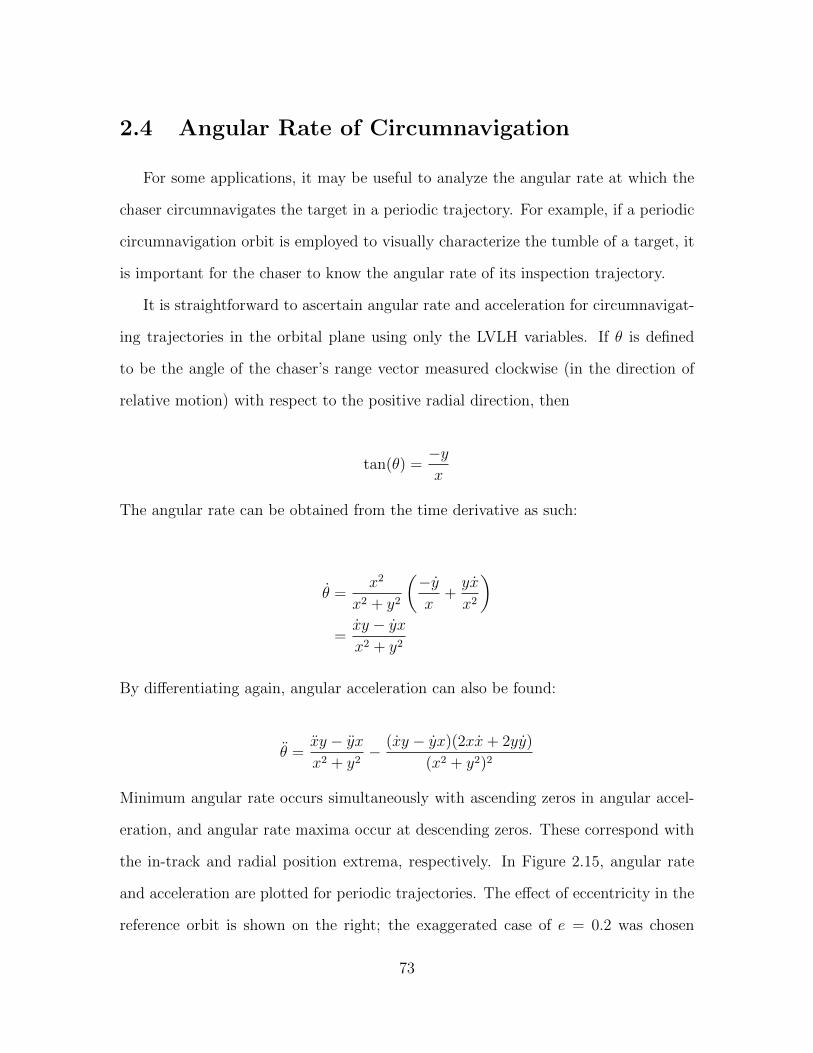
2.4 Angular Rate of Circumnavigation

For some applications, it may be useful to analyze the angular rate at which the

chaser circumnavigates the target in a periodic trajectory. For example, if a periodic

circumnavigation orbit is employed to visually characterize the tumble of a target, it

is important for the chaser to know the angular rate of its inspection trajectory.

It is straightforward to ascertain angular rate and acceleration for circumnavigat-

ing trajectories in the orbital plane using only the LVLH variables. If θ is defined

to be the angle of the chaser’s range vector measured clockwise (in the direction of

relative motion) with respect to the positive radial direction, then

tan(θ) =−yx

The angular rate can be obtained from the time derivative as such:

θ =x2

x2 + y2

(−yx

+yx

x2

)=xy − yxx2 + y2

By differentiating again, angular acceleration can also be found:

θ =xy − yxx2 + y2

− (xy − yx)(2xx+ 2yy)

(x2 + y2)2

Minimum angular rate occurs simultaneously with ascending zeros in angular accel-

eration, and angular rate maxima occur at descending zeros. These correspond with

the in-track and radial position extrema, respectively. In Figure 2.15, angular rate

and acceleration are plotted for periodic trajectories. The effect of eccentricity in the

reference orbit is shown on the right; the exaggerated case of e = 0.2 was chosen

73

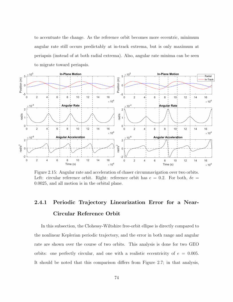
to accentuate the change. As the reference orbit becomes more eccentric, minimum

angular rate still occurs predictably at in-track extrema, but is only maximum at

periapsis (instead of at both radial extrema). Also, angular rate minima can be seen

to migrate toward periapsis.

0 2 4 6 8 10 12 14 16

104

-5

0

5

Pos

ition

(m

)

105 In-Plane MotionRadial

In-Track

0 2 4 6 8 10 12 14 16

104

0

1

2

rad/

s

10-4 Angular Rate

0 2 4 6 8 10 12 14 16

Time (s) 104

-2

0

2

rad/

s2

10-8 Angular Acceleration

0 2 4 6 8 10 12 14 16

104

-5

0

5

Pos

ition

(m

)

105 In-Plane Motion

0 2 4 6 8 10 12 14 16

104

0

1

2

rad/

s

10-4 Angular Rate

0 2 4 6 8 10 12 14 16

Time (s) 104

-2

0

2

rad/

s2

10-8 Angular Acceleration

Figure 2.15: Angular rate and acceleration of chaser circumnavigation over two orbits.Left: circular reference orbit. Right: reference orbit has e = 0.2. For both, δe =0.0025, and all motion is in the orbital plane.

2.4.1 Periodic Trajectory Linearization Error for a Near-

Circular Reference Orbit

In this subsection, the Clohessy-Wiltshire free-orbit ellipse is directly compared to

the nonlinear Keplerian periodic trajectory, and the error in both range and angular

rate are shown over the course of two orbits. This analysis is done for two GEO

orbits: one perfectly circular, and one with a realistic eccentricity of e = 0.005.

It should be noted that this comparison differs from Figure 2.7; in that analysis,

74

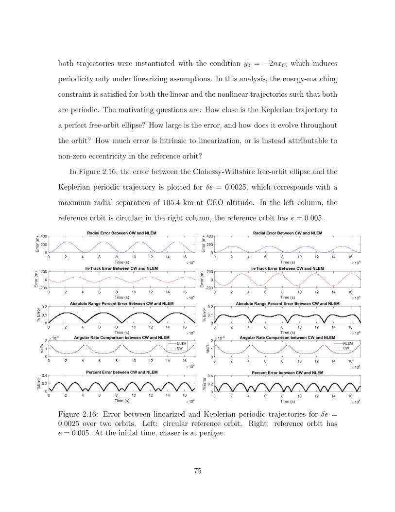
both trajectories were instantiated with the condition y0 = −2nx0, which induces

periodicity only under linearizing assumptions. In this analysis, the energy-matching

constraint is satisfied for both the linear and the nonlinear trajectories such that both

are periodic. The motivating questions are: How close is the Keplerian trajectory to

a perfect free-orbit ellipse? How large is the error, and how does it evolve throughout

the orbit? How much error is intrinsic to linearization, or is instead attributable to

non-zero eccentricity in the reference orbit?

In Figure 2.16, the error between the Clohessy-Wiltshire free-orbit ellipse and the

Keplerian periodic trajectory is plotted for δe = 0.0025, which corresponds with a

maximum radial separation of 105.4 km at GEO altitude. In the left column, the

reference orbit is circular; in the right column, the reference orbit has e = 0.005.

0 2 4 6 8 10 12 14 16

Time (s) 104

0

200

400

Err

or (

m)

Radial Error Between CW and NLEM

0 2 4 6 8 10 12 14 16

Time (s) 104

-200

0

200

Err

or (

m)

In-Track Error Between CW and NLEM

0 2 4 6 8 10 12 14 16

Time (s) 104

0

0.1

0.2

% E

rror

Absolute Range Percent Error Between CW and NLEM

0 2 4 6 8 10 12 14 16

Time (s) 104

0

200

400

Err

or (

m)

Radial Error Between CW and NLEM

0 2 4 6 8 10 12 14 16

Time (s) 104

-200

0

200

Err

or (

m)

In-Track Error Between CW and NLEM

0 2 4 6 8 10 12 14 16

Time (s) 104

0

0.1

0.2

% E

rror

Absolute Range Percent Error Between CW and NLEM

0 2 4 6 8 10 12 14 16

104

0

1

2

rad/

s

10-4 Angular Rate Comparison between CW and NLEM

NLEM

CW

0 2 4 6 8 10 12 14 16

Time (s) 104

0

0.2

0.4

%E

rro

r

Percent Error between CW and NLEM

0 2 4 6 8 10 12 14 16

104

0

1

2

rad/

s

10-4 Angular Rate Comparison between CW and NLEMNLEM

CW

0 2 4 6 8 10 12 14 16

Time (s) 104

0

0.2

0.4

%E

rro

r

Percent Error between CW and NLEM

Figure 2.16: Error between linearized and Keplerian periodic trajectories for δe =0.0025 over two orbits. Left: circular reference orbit. Right: reference orbit hase = 0.005. At the initial time, chaser is at perigee.

75

This analysis indicates that even with a perfectly circular reference orbit, the

Clohessy-Wiltshire ellipse is hundreds of meters in error with respect to its periodic

Keplerian counterpart. Introducing a small amount of eccentricity changes the shape

of the error curve, but does not substantially change the magnitude of the range error.

Likewise, angular rate error is affected only subtly by realistic eccentricity, with only

a slight increase at the radial maxima. It is interesting to note that the characteristic

of both range and angular rate errors is periodic, with range error ‘minima’ occuring

along the radial axis (Figure 2.10 corroborates this).

In Figure 2.17, linearization error is depicted for a closer-range periodic trajectory;

this time, δe = 2.5 × 10−5, corresponding to a maximum radial separation of only

1.054 km.

0 2 4 6 8 10 12 14 16

104

0

1

2

rad/

s

10-4 Angular Rate Comparison between CW and NLEM

NLEM

CW

0 2 4 6 8 10 12 14 16

Time (s) 104

0

0.05

0.1

%E

rro

r

Percent Error between CW and NLEM

0 2 4 6 8 10 12 14 16

Time (s) 104

-1.5-1

-0.50

0.5

Err

or (

m)

Radial Error Between CW and NLEM

0 2 4 6 8 10 12 14 16

Time (s) 104

-1

0

1

Err

or (

m)

In-Track Error Between CW and NLEM

0 2 4 6 8 10 12 14 16

Time (s) 104

0

0.05

0.1

% E

rror

Absolute Range Percent Error Between CW and NLEM

0 2 4 6 8 10 12 14 16

104

0

1

2

rad/

s

10-4 Angular Rate Comparison between CW and NLEM

NLEM

CW

0 2 4 6 8 10 12 14 16

Time (s) 104

0

0.05

0.1

%E

rro

r

Percent Error between CW and NLEM

0 2 4 6 8 10 12 14 16

Time (s) 104

-1.5-1

-0.50

0.5

Err

or (

m)

Radial Error Between CW and NLEM

0 2 4 6 8 10 12 14 16

Time (s) 104

-1

0

1

Err

or (

m)

In-Track Error Between CW and NLEM

0 2 4 6 8 10 12 14 16

Time (s) 104

0

0.05

0.1

% E

rror

Absolute Range Percent Error Between CW and NLEM

Figure 2.17: Error between linearized and Keplerian periodic trajectories for δe =2.5 × 10−5 over two orbits. Left: circular reference orbit. Right: reference orbit hase = 0.005. At the initial time, chaser is at perigee.

76

Interestingly, for this close of a periodic trajectory to a target in a perfectly cir-

cular orbit, error is relatively small between the Clohessy-Wiltshire ellipse and the

Keplerian energy-matched trajectory. The introduction of realistic eccentricity in-

creases the error by an order of magnitude. This shows that the linearization error

for close-range periodic trajectories are much more sensitive to eccentricity than far-

range trajectories.

This analysis shows that the free-orbit ellipse is not a perfect descriptor of periodic

relative motion, even in the absence of orbit perturbations. Error accumulates due to

range from the target; however, in these large (100-200km) trajectories, small vari-

ations of target eccentricity do not significantly contribute to error. For close-range

(1-2km) trajectories, it would appear that the free-orbit ellipse is a good descrip-

tor of motion, but only for perfectly circular target orbits; with realistic eccentricity

considered, however, error increases to approximately half that of a 100-times-larger

trajectory. For long duration proximity operations which spend protracted amounts

of time at these ranges, the continuous accumulation of this error could be unaccept-

able.

This analysis also reveals the characteristics of the error over the course of the

orbit. The range error is periodic, with minima occurring at apogee and perigee

(along the radial axis). This implies that the free-orbit ellipse is most accurate at

these points in the orbit. Circumnavigational angular rate error is also periodic, but

minima occur at the maximum in-track separation (as well as on either side of apogee

and perigee for the larger trajectory). The knowledge of the timing of these points

at which a periodic trajectory is approximated with near-zero error by the simple

free-orbit ellipse, at least in the case of Keplerian spherical gravity, could be useful

for long-duration formation fliers.

77

2.5 Effects of Orbit Perturbations on Relative Dy-

namics

Orbital perturbations were introduced near the beginning of this chapter, but they

have been ignored since then in the interest of developing an understanding of the

nuances of linearizing relative motion under ideal, spherical-gravity conditions. Or-

bital perturbations are any effects that cause the ideally constant Keplerian elements

of an orbit to change over time. If the Keplerian elements do not remain constant,

the nonlinear equations of relative motion (which were a direct consequence of pure

Two-Body motion) no longer hold in the form presented above. However, they can

easily be modified to include accelerations due to external forces, which is a common

way to model orbital perturbations:

x = 2νy + νy + ν2x+µ

r2tgt− µ

r3ch(rtgt + x) + ax

y = −2νx− νx+ ν2y − µ

r3ch(y) + ay

z = − µ

r3ch(z) + az

The same approach is also easily taken with the Clohessy-Wiltshire equations:

x = 2ny + 3n2x+ ax

y = −2nx+ ay

z = −n2z + az

For some types of perturbations, it is somewhat straightforward to include their

78

effects in this way. One example is a simplified consideration of atmospheric drag,

which can be modeled as a force that opposes the velocity of the spacecraft with

respect to the atmosphere at any given time. If the chaser and target have the same

ballistic coefficient, air drag affects both spacecraft identically; the only effect it would

have on the chaser would be in the form of ‘differential’ air drag, a function of ˙ρ.

Schaub and Alfriend [32] found the effect of differential air drag on LEO formation

fliers to be of negligible impact on relative motion compared to oblate-Earth effects

(J2). As is described in Appendix A, J2 perturbations cause apsidal rotation (∆ω)

and nodal regression (∆Ω), and are functions of semimajor axis, eccentricity, and

inclination. In effect, this means there is nearly always a relative differential J2 force

acting on the chaser if it is not stationary on the target’s orbital trajectory. In general,

it manifests itself as a secular in-track drift [29].

There are certain conditions that, when met, cause the chaser and target to share

the same magnitude of secular in-track drift caused by J2 perturbations in the LVLH

frame; the result is referred to as a ‘J2-invariant’ relative trajectory. The following

necessary conditions on semimajor axis, eccentricity, and inclination developed by

Schaub, et al. [32], which were formulated from Brouwer’s analytical solution to the

Two-Body problem with zonal harmonics, must be met in order for the relative motion

to be J2-invariant to first order:

δa = 2Datgtδη

δη = −1

4ηtgtδi tan(itgt)

Where,

η =√

1− e2 =h

µ2a2

79

D =J2

4a2tgtη5tgt

(4 + 3ηtgt)(1 + 5 cos2(itgt))

If a periodic relative trajectory is desired, it was previously shown that the energy-

matching constraint must be met between the chaser and target orbits, which implies

δa = 0. This severely constrains the space of periodic J2-invariant orbits. One way

to meet the requirement is to have δη = 0. The fact that the chaser and target

must share the same η and that eccentricity can only be positive or zero means that

ech = etgt, which is the degenerate case where the chaser lies stationary on the target’s

orbital trajectory.

In this first-order approximation of the oblate-Earth gravity field, it appears that

there cannot exist a (non-trivial) periodic relative trajectory. However, it may be

possible to ‘counteract’ J2 effects on average by relaxing the constraint that δa = 0,

allowing a mismatch in energy to be balanced by the secular drift caused by the

perturbation. The resulting motion would not be perfectly periodic, but pseudo-

periodic in a bounded fashion. This complex motion won’t be analyzed in this thesis,

but other research and numerical analyses suggest that there exist combinations of

orbital elements that admit J2-invariant bounded relative motion. [4] [32] [21] [37] [1]

The altitude regime of the orbit plays a significant role in the types and magni-

tudes of perturbations that dominate. For example, in a 200-km-altitude LEO orbit,

differential drag will likely be the biggest foe. However, moving upwards toward GEO,

drag virtually disappears and J2 effects diminish, while solar radiation pressure and

third-body gravitation from the sun and moon begin to dominate [3]. It is possible

to model these external gravitational accelerations using the Three-Body problem, of

which Vallado provides a treatment [38].

80

2.6 Chapter Summary

This chapter explored the orbit mechanical basis for proximity operations, intro-

ducing the LVLH coordinate frame and deriving the nonlinear Keplerian equations

of relative motion, then linearizing those to obtain the common Clohessy-Wiltshire

equations and their solutions. The linearizing and simplifying steps were carefully

noted, and the effects of linearization on range error was explored for a variety of sce-

narios; in essence, the curved orbit trajectory is assumed to be a line in the linearized

model, so error grows quickly with the magnitude of range. While the Clohessy-

Wiltshire equations of motion have small error with Keplerian motion at close range

and for short time scales, they are less well-suited to proximity operations not in the

‘terminal phase,’ such as extended formation flight or inspection.

Methods for specifying the size, position, and orientation of relative trajectories

in the periodic class are presented in the form of constraints over the LVLH vari-

ables for both the Clohessy-Wiltshire and the Keplerian models. Also, a formula for

the angular rate and acceleration of in-plane circumnavigation in the LVLH state

variables was given. The ‘cost of linearization’ analysis was revisited for periodic

trajectories, showing how the time evolution of error changes shape and magnitude

for perfectly circular and near-circular reference orbits and for medium-range and

close-range proximity operations. From this analysis, it was concluded that realis-

tic eccentricity disrupts the accuracy of the linearized model at close-range far more

than at medium-range, but the overall error in the medium-range was largest in both

the circular and near-circular cases. It was also identified that the periodic nature

of the error results in an ‘osculation’ behavior over the course of the orbit, showing

that the linearized model is most accurate in range at the maximum and minimum

radial offset, and is most accurate in angular rate of circumnavigation at maximum

81

and minimum in-track offset. Thus, there are two points in every orbit where range

and rate measurements should agree closely with the linearized model, even if the

reference orbit is not perfectly circular.

Lastly, the effect of orbit perturbations on relative motion was briefly discussed.

Since perturbations change the Keplerian elements of an orbit, and because pertur-

bations affect the chaser and target differently, they render the nonlinear Keplerian

model invalid. J2 causes a secular in-track drift even for energy-matched relative tra-

jectories at all inclinations except the critical inclination, but the magnitude of this

perturbative effect decreases with orbit altitude. In GEO regimes, the more chaotic

third-body effects from the Sun and moon dominate over J2 and drag.

In the next chapter, techniques for minimizing time, fuel, or energy during satellite

proximity operations is explored both analytically and numerically. Similarly to the

findings of this chapter, Clohessy-Wiltshire dynamics make the problem simpler to

analyze, but at the cost of realism in the result. The desire to use higher-fidelity ac-

celeration models (such as the Keplerian relative motion model) or to couple attitude

dynamics with the problem introduce nonlinearities that warrant implementation in

a numerical optimization framework.

82

Chapter 3

Optimal Control ProblemFormulation

The optimal control problem is first introduced in the simplest form possible, as a

bounded-control MIMO state regulation problem (rendezvous) in the relative carte-

sian coordinate frame with LTI dynamics. This allows a straightforward analytical

solution for the optimal control to be developed for a variety of objective functions,

which is useful to validate the more general tool used to generate optimal trajecto-

ries for long-duration proximity operations in Chapter 4. Additionally, the presence

of singular solutions in the control is investigated with an interesting result for the

minimum-time problem. The proximity operations problem is then expanded to a

larger state space that additionally describes the attitude dynamics of a spacecraft

with a single body-mounted propulsion device.

In the second half of this chapter, the Rendezvous / Proximity Operations Tra-

jectory Analysis Tool is introduced. This numerical optimization framework uses

GPOPS-II [30], an adaptive-mesh pseudospectral collocation optimization software

in MATLAB, along with the open-source nonlinear program solver IPOPT [39] to

analyze a rich variety of relevant proximity operations problems. This tool is vali-

dated and applied to long-duration proximity operations in the Results chapter.

83

3.1 The Optimal Control Problem

Principles of optimal control are especially relevant to spacecraft engineering be-

cause of the challenging and inaccessible nature of operating in the space environment.

Formation fliers and on-orbit servicers can greatly extend their mission lifetimes by

employing these principles to minimize fuel use. Other satellites may need to respond

quickly to various circumstances, minimizing the time to reach a certain point or

trajectory. This section contains a brief overview of several different formulations of

the optimal trajectory control problem for spacecraft rendezvous.

Throughout the following section, the state vector will be denoted x (which should

be kept distinct from the radial coordinate from the previous section), the costate

vector will be denoted p, the control input vector will be denoted u, and the objective

function will be denoted J .

3.1.1 The 3-DOF Formulation

The simplest way to form the optimal control problem for spacecraft proximity

operations is to treat the chaser as an unchanging point mass that can provide limited

thrust in each coordinate of the LVLH frame. The system to be controlled can then

be expressed in six states: the relative position and the relative velocity between the

two spacecraft.

84

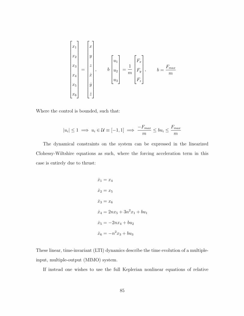
x1

x2

x3

x4

x5

x6

=

x

y

z

x

y

z

, b

u1

u2

u3

=1

m

Fx

Fy

Fz

, b =Fmaxm

Where the control is bounded, such that:

|ui| ≤ 1 =⇒ ui ∈ U ≡ [−1, 1] =⇒ −Fmaxm

≤ bui ≤Fmaxm

The dynamical constraints on the system can be expressed in the linearized

Clohessy-Wiltshire equations as such, where the forcing acceleration term in this

case is entirely due to thrust:

x1 = x4

x2 = x5

x3 = x6

x4 = 2nx5 + 3n2x1 + bu1

x5 = −2nx4 + bu2

x6 = −n2x3 + bu3

These linear, time-invariant (LTI) dynamics describe the time evolution of a multiple-

input, multiple-output (MIMO) system.

If instead one wishes to use the full Keplerian nonlinear equations of relative

85

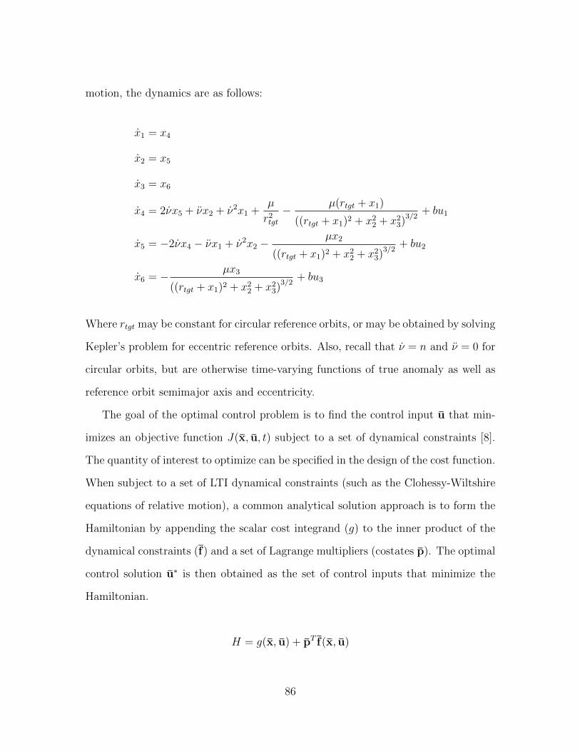
motion, the dynamics are as follows:

x1 = x4

x2 = x5

x3 = x6

x4 = 2νx5 + νx2 + ν2x1 +µ

r2tgt− µ(rtgt + x1)

((rtgt + x1)2 + x22 + x23)3/2

+ bu1

x5 = −2νx4 − νx1 + ν2x2 −µx2

((rtgt + x1)2 + x22 + x23)3/2

+ bu2

x6 = − µx3

((rtgt + x1)2 + x22 + x23)3/2

+ bu3

Where rtgt may be constant for circular reference orbits, or may be obtained by solving

Kepler’s problem for eccentric reference orbits. Also, recall that ν = n and ν = 0 for

circular orbits, but are otherwise time-varying functions of true anomaly as well as

reference orbit semimajor axis and eccentricity.

The goal of the optimal control problem is to find the control input u that min-

imizes an objective function J(x, u, t) subject to a set of dynamical constraints [8].

The quantity of interest to optimize can be specified in the design of the cost function.

When subject to a set of LTI dynamical constraints (such as the Clohessy-Wiltshire

equations of relative motion), a common analytical solution approach is to form the

Hamiltonian by appending the scalar cost integrand (g) to the inner product of the

dynamical constraints (f) and a set of Lagrange multipliers (costates p). The optimal

control solution u∗ is then obtained as the set of control inputs that minimize the

Hamiltonian.

H = g(x, u) + pT f(x, u)

86

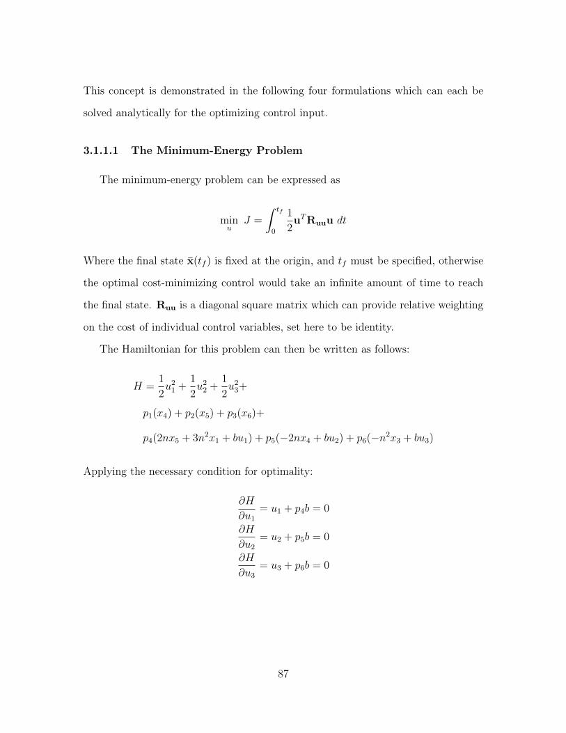
This concept is demonstrated in the following four formulations which can each be

solved analytically for the optimizing control input.

3.1.1.1 The Minimum-Energy Problem

The minimum-energy problem can be expressed as

minu

J =

∫ tf

0

1

2uTRuuu dt

Where the final state x(tf ) is fixed at the origin, and tf must be specified, otherwise

the optimal cost-minimizing control would take an infinite amount of time to reach

the final state. Ruu is a diagonal square matrix which can provide relative weighting

on the cost of individual control variables, set here to be identity.

The Hamiltonian for this problem can then be written as follows:

H =1

2u21 +

1

2u22 +

1

2u23+

p1(x4) + p2(x5) + p3(x6)+

p4(2nx5 + 3n2x1 + bu1) + p5(−2nx4 + bu2) + p6(−n2x3 + bu3)

Applying the necessary condition for optimality:

∂H

∂u1= u1 + p4b = 0

∂H

∂u2= u2 + p5b = 0

∂H

∂u3= u3 + p6b = 0

87

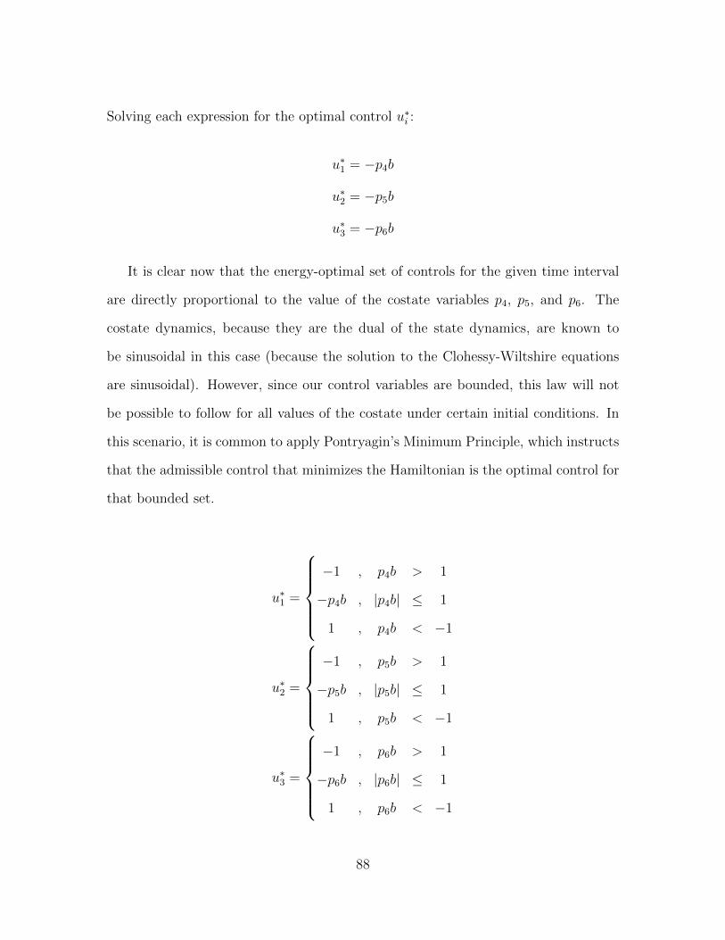
Solving each expression for the optimal control u∗i :

u∗1 = −p4b

u∗2 = −p5b

u∗3 = −p6b

It is clear now that the energy-optimal set of controls for the given time interval

are directly proportional to the value of the costate variables p4, p5, and p6. The

costate dynamics, because they are the dual of the state dynamics, are known to

be sinusoidal in this case (because the solution to the Clohessy-Wiltshire equations

are sinusoidal). However, since our control variables are bounded, this law will not

be possible to follow for all values of the costate under certain initial conditions. In

this scenario, it is common to apply Pontryagin’s Minimum Principle, which instructs

that the admissible control that minimizes the Hamiltonian is the optimal control for

that bounded set.

u∗1 =

−1 , p4b > 1

−p4b , |p4b| ≤ 1

1 , p4b < −1

u∗2 =

−1 , p5b > 1

−p5b , |p5b| ≤ 1

1 , p5b < −1

u∗3 =

−1 , p6b > 1

−p6b , |p6b| ≤ 1

1 , p6b < −1

88

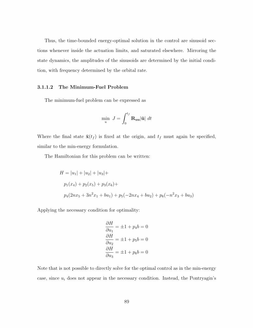
Thus, the time-bounded energy-optimal solution in the control are sinusoid sec-

tions whenever inside the actuation limits, and saturated elsewhere. Mirroring the

state dynamics, the amplitudes of the sinusoids are determined by the initial condi-

tion, with frequency determined by the orbital rate.

3.1.1.2 The Minimum-Fuel Problem

The minimum-fuel problem can be expressed as

minu

J =

∫ tf

0

Ruu|u| dt

Where the final state x(tf ) is fixed at the origin, and tf must again be specified,

similar to the min-energy formulation.

The Hamiltonian for this problem can be written:

H = |u1|+ |u2|+ |u3|+

p1(x4) + p2(x5) + p3(x6)+

p4(2nx5 + 3n2x1 + bu1) + p5(−2nx4 + bu2) + p6(−n2x3 + bu3)

Applying the necessary condition for optimality:

∂H

∂u1= ±1 + p4b = 0

∂H

∂u2= ±1 + p5b = 0

∂H

∂u3= ±1 + p6b = 0

Note that is not possible to directly solve for the optimal control as in the min-energy

case, since ui does not appear in the necessary condition. Instead, the Pontryagin’s

89

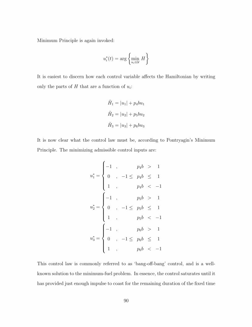
Minimum Principle is again invoked:

u∗i (t) = arg

minui∈U

H

It is easiest to discern how each control variable affects the Hamiltonian by writing

only the parts of H that are a function of ui:

H1 = |u1|+ p4bu1

H2 = |u2|+ p5bu2

H3 = |u3|+ p6bu3

It is now clear what the control law must be, according to Pontryagin’s Minimum

Principle. The minimizing admissible control inputs are:

u∗1 =

−1 , p4b > 1

0 , −1 ≤ p4b ≤ 1

1 , p4b < −1

u∗2 =

−1 , p5b > 1

0 , −1 ≤ p5b ≤ 1

1 , p5b < −1

u∗3 =

−1 , p6b > 1

0 , −1 ≤ p6b ≤ 1

1 , p6b < −1

This control law is commonly referred to as ‘bang-off-bang’ control, and is a well-

known solution to the minimum-fuel problem. In essence, the control saturates until it

has provided just enough impulse to coast for the remaining duration of the fixed time

90

interval, then performs a mirroring thrust in the opposite direction at the maneuver

terminus.

3.1.1.3 The Minimum-Time Problem

The minimum-time problem can be expressed as

minu

J =

∫ tf

0

1 dt

Where the final state x(tf ) is fixed at the origin, but tf is left as a free parameter

(since it is the quantity that is being optimized).

The Hamiltonian for this problem can be written as follows:

H = 1+p1(x4)+p2(x5)+p3(x6)+p4(2nx5+3n2x1+bu1)+p5(−2nx4+bu2)+p5(−n2x3+bu3)

Applying the necessary condition for optimality:

∂H

∂u1= p4b = 0

∂H

∂u2= p5b = 0

∂H

∂u3= p6b = 0

However, since the control ui once again appears linearly in the Hamiltonian, the op-

timal control cannot be explicitly determined from this condition alone. Pontryagin’s

Minimum Principle states:

u∗i (t) = arg

minui∈U

H

91

The part of the Hamiltonian which depends on ui can be written:

H = p4bu1 + p5bu2 + p6bu3

Thus, given the constraint on the control, and the fact that b is a strictly positive

constant, the familiar and expected ‘bang-bang’ control law satisfies the Minimum

Principle:

u1 =

−1 , p4 > 0

1 , p4 < 0

u2 =

−1 , p5 > 0

1 , p5 < 0

u3 =

−1 , p6 > 0

1 , p6 < 0

3.1.2 Determining the Existence of Singular Arcs in the So-

lution

As useful as Pontryagin’s Minimum Principle can be in its generality, it sometimes

fails to define the optimal control for the entire range of possible scenarios. There

are certain cases where extremal control is not in fact the solution for minimum-time

problems; instead, an intermediate or ‘singular’ control may be optimal for certain

sections or ‘arcs’ in the problem [25]. a notable example of this is the minimum time

to ascend for a rocket in atmosphere (the Goddard rocket problem), for which an

intermediate thrust at a certain altitude range results in the fastest ascent due to a

balancing of linear acceleration and aerodynamic drag. Many optimization problems

92

with nonlinear dynamics as such have solutions which feature singular arcs; as a

general rule, however, SISO min-time problems with LTI dynamics do not feature

arcs of singular control in the solution.

However, the possibility of a singular arc in the control for the Min-Time problem

formulation can be superficially observed because the optimal control law is undefined

when p4, p5, or p6 are equal to zero for some finite amount of time. Boyarko, et al.

identified, but did not fully explore, this possibility for the minimum-time rendezvous

problem [6]. This situation, where the Hamiltonian is linear in the control variable

and the coefficient on it may be zero for finite time, is a typical one in which singular

arcs can be found in optimal control problems [25]. The key is to identify whether it is

possible for this coefficient – in this case, the velocity costates – to be identically zero

for finite time in the problem. For a SISO system (e.g., if only one coordinate were

being regulated), this would not occur, because velocity is never zero until the end

of the problem (thus, the costate is only instantaneously zero at the final moment).

In fact, since the solution to the dynamics is known to be a forced sinusoid, the only

situation in which the costate is zero for finite time is in the case when velocity is

zero at the coordinate origin (a zero-amplitude, zero-bias sinusoid).

For the 3-DOF MIMO problem, however, it is not only possible but nearly un-

avoidable for some costates to be identically zero for finite time before the problem

terminus. This occurs whenever either the in-plane or out-of-plane coordinates are

regulated to their origin before the others. Instead of requiring intermediate thrust

as in the case of the Goddard rocket problem, the result is actually a “degenerate

class of singular solutions” in the sense of J.P. LaSalle [26].

In essence, this is a ‘scheduling ambiguity,’ where a single unique solution to the

min-time problem does not exist unless extremal control can regulate both in-plane

and out-of-plane coordinates in precisely the same amount of time. For the vast

93

majority of initial conditions, this will not be the case, and one or the other will

be regulated to the coordinate origin(s) first with a waiting period until the limiting

coordinate is regulated. The non-uniqueness of the solution is easily understood when

considering that an equally optimal solution would be to begin regulating the limiting

coordinate first, waiting until the last possible moment to regulate the non-limiting

coordinate; and also equally optimal is any scheduling of non-limiting coordinate

regulation between this time and the initial time.

This scheduling ambiguity is easily resolved by simply choosing a scheduling policy,

for example, ‘regulate, then wait,’ or ’wait, then regulate.’ This arbitration effectively

chooses a unique solution from the degenerate class, resolving the ambiguity. A

more interesting resolution to this ambiguity is to instead adopt a hybrid policy,

where extremal control is executed for the limiting coordinate while the non-limiting

coordinate is optimized for minimum fuel or energy use, with final time specified as the

minimum regulation time for the limiting coordinate. The result is still time-optimal

given the actuator saturation bounds, but more efficient with on-board resources, and

there is only one unique solution.

Scheduling ambiguity in the solution to the Min-Time problem is not particularly

intuitive. A human’s solution would likely be to travel in a relatively straight line to

the target, utilizing a bang-bang strategy. The fact that it crops up here is actually

an artifact of the rudimentary formulation of the problem, which treats all control

inputs as independently-saturating thrusters locked in the direction of the coordinate

axes (frame-component saturation). This is tantamount to a cubical satellite with a

thruster mounted on each side panel holding its attitude such that each thruster is

aligned with an LVLH axis. If such a satellite needed to minimize time to rendezvous,

the solution would be to slew such that the combined thrust from three nozzles created

a single larger thrust vector, which would be pointed more or less directly at the target

94

and used in a bang-bang fashion. This concept is depicted in section 3.2.

The exploration of the possibility of singular arcs in the minimum-time problem

revealed the somewhat trivial result that scheduling ambiguity exists in the 3-DOF

formulation of the problem. This exercise was useful because it underscores the

degree to which a minimum-time MIMO 3-DOF rendezvous problem formulation is

unrealistic. It also motivates a dynamics framework that couples position and attitude

to adequately represent certain types of maneuvers in satellite proximity operations.

3.1.3 Including Attitude Dynamics: The 6-DOF Formulation

The 6-DOF problem formulation presented here features a satellite with three

independently-saturating reaction wheels and only one thruster. The satellite must

use the reaction wheels to point the thrust vector in the appropriate direction for

motion. The result is a system for which translation and rotation are coupled; the

vehicle may only accelerate in the direction that it is pointing.

The problem’s state vector expands to include four quaternions for attitude rep-

resentation and three body angular rates:

x = [x y z x y z q1 q2 q3 q4 ω1 ω2 ω3]T

The inputs are the single thruster’s throttle, which may vary from 0 (off) to 1 (fully

saturated), and the three reaction wheel torques, which may vary from -1 to 1:

u =[uF uτx uτy uτz

]TQuaternions are chosen over Euler angles to avoid gimbal lock and for the ease of

implementation into the numerical solver. The attitude state quaternion q resolves

95

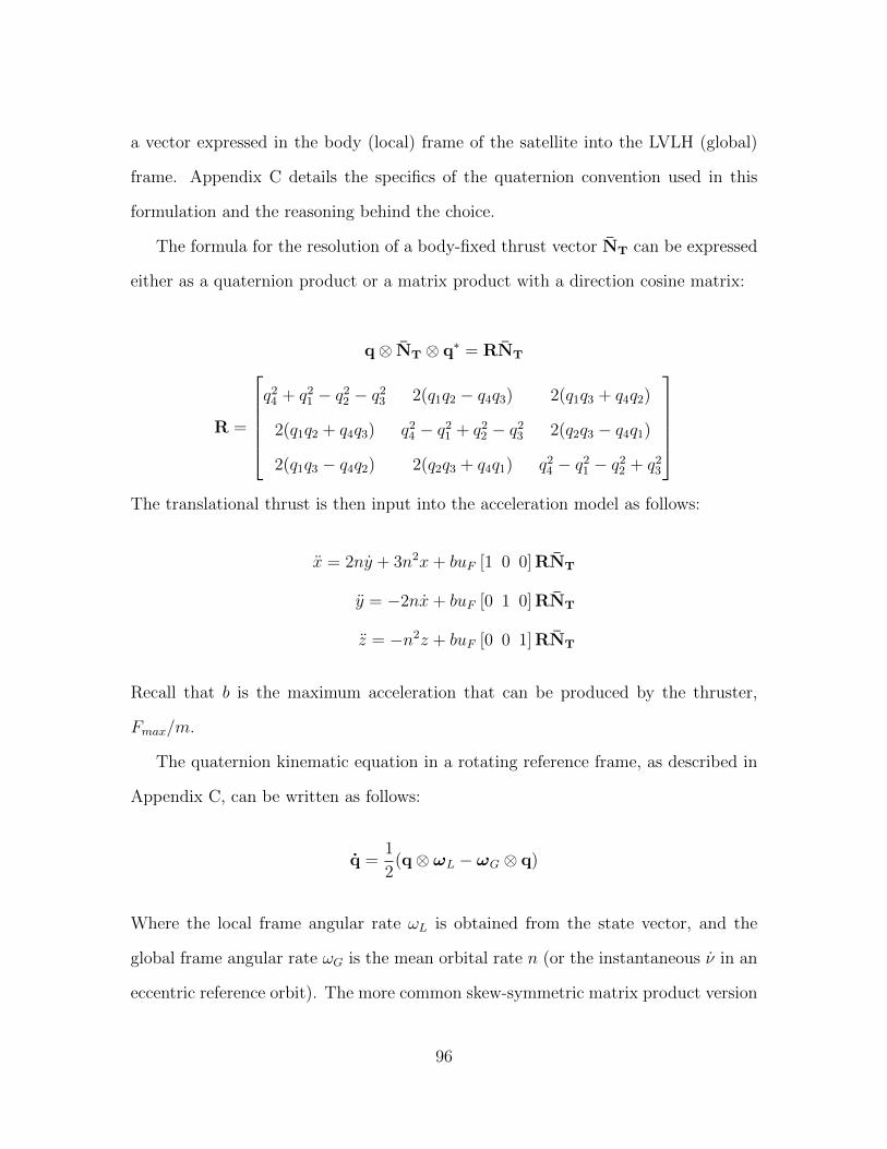
a vector expressed in the body (local) frame of the satellite into the LVLH (global)

frame. Appendix C details the specifics of the quaternion convention used in this

formulation and the reasoning behind the choice.

The formula for the resolution of a body-fixed thrust vector NT can be expressed

either as a quaternion product or a matrix product with a direction cosine matrix:

q⊗ NT ⊗ q∗ = RNT

R =

q24 + q21 − q22 − q23 2(q1q2 − q4q3) 2(q1q3 + q4q2)

2(q1q2 + q4q3) q24 − q21 + q22 − q23 2(q2q3 − q4q1)

2(q1q3 − q4q2) 2(q2q3 + q4q1) q24 − q21 − q22 + q23

The translational thrust is then input into the acceleration model as follows:

x = 2ny + 3n2x+ buF [1 0 0] RNT

y = −2nx+ buF [0 1 0] RNT

z = −n2z + buF [0 0 1] RNT

Recall that b is the maximum acceleration that can be produced by the thruster,

Fmax/m.

The quaternion kinematic equation in a rotating reference frame, as described in

Appendix C, can be written as follows:

q =1

2(q⊗ ωL − ωG ⊗ q)

Where the local frame angular rate ωL is obtained from the state vector, and the

global frame angular rate ωG is the mean orbital rate n (or the instantaneous ν in an

eccentric reference orbit). The more common skew-symmetric matrix product version

96

of this kinematic equation is also described in the appendix.

Rigid-body rate dynamics are given by Euler’s moment equations with reaction

wheel torque inputs as forcing terms:

ωx = I−1xx [(Iyy − Izz)ωyωz + τmaxuτx ]

ωy = I−1yy[(Izz − Ixx)ωxωz + τmaxuτy

]ωz = I−1zz [(Ixx − Iyy)ωxωy + τmaxuτz ]

Where the inertia matrix I is assumed to be diagonal and constant, and τmax is the

greatest torque magnitude that can be supplied by the reaction wheel.

Taking the thrust vector direction to be NT = [1 0 0]T , and evaluating the matrix

and quaternion products, the full state dynamics can be written as follows:

97

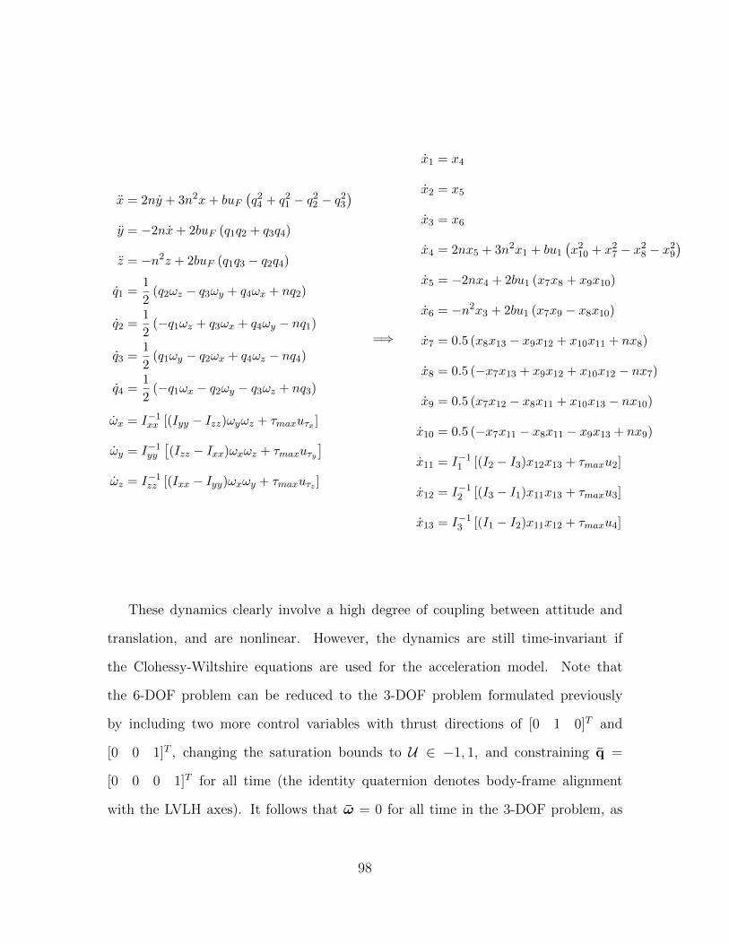
x = 2ny + 3n2x+ buF(q24 + q21 − q22 − q23

)y = −2nx+ 2buF (q1q2 + q3q4)

z = −n2z + 2buF (q1q3 − q2q4)

q1 =1

2(q2ωz − q3ωy + q4ωx + nq2)

q2 =1

2(−q1ωz + q3ωx + q4ωy − nq1)

q3 =1

2(q1ωy − q2ωx + q4ωz − nq4)

q4 =1

2(−q1ωx − q2ωy − q3ωz + nq3)

ωx = I−1xx [(Iyy − Izz)ωyωz + τmaxuτx ]

ωy = I−1yy[(Izz − Ixx)ωxωz + τmaxuτy

]ωz = I−1zz [(Ixx − Iyy)ωxωy + τmaxuτz ]

=⇒

x1 = x4

x2 = x5

x3 = x6

x4 = 2nx5 + 3n2x1 + bu1(x210 + x27 − x28 − x29

)x5 = −2nx4 + 2bu1 (x7x8 + x9x10)

x6 = −n2x3 + 2bu1 (x7x9 − x8x10)

x7 = 0.5 (x8x13 − x9x12 + x10x11 + nx8)

x8 = 0.5 (−x7x13 + x9x12 + x10x12 − nx7)

x9 = 0.5 (x7x12 − x8x11 + x10x13 − nx10)

x10 = 0.5 (−x7x11 − x8x11 − x9x13 + nx9)

x11 = I−11 [(I2 − I3)x12x13 + τmaxu2]

x12 = I−12 [(I3 − I1)x11x13 + τmaxu3]

x13 = I−13 [(I1 − I2)x11x12 + τmaxu4]

These dynamics clearly involve a high degree of coupling between attitude and

translation, and are nonlinear. However, the dynamics are still time-invariant if

the Clohessy-Wiltshire equations are used for the acceleration model. Note that

the 6-DOF problem can be reduced to the 3-DOF problem formulated previously

by including two more control variables with thrust directions of [0 1 0]T and

[0 0 1]T , changing the saturation bounds to U ∈ −1, 1, and constraining q =

[0 0 0 1]T for all time (the identity quaternion denotes body-frame alignment

with the LVLH axes). It follows that ω = 0 for all time in the 3-DOF problem, as

98

well. Note that this would enlarge the control vector to a length of six, and the matrix

product coupling translation inputs with attitude would need to be recomputed.

The inclusion of coupling attitude dynamics adds a layer of complexity to the

problem which makes it more difficult to analyze than the 3-DOF formulation, but it

may be the most realistic framing of the problem in some circumstances. This notion

is further explored in the next section.

3.2 Insights Gained from Preliminary Analysis

3.2.1 Over-Actuation in the Problem Formulation

In the linearized dynamics, motion in the in-plane and out-of-plane coordinates are

uncoupled. This means that the system is still fully controllable when simultaneous

in-plane and out-of-plane actuation is possible (for example, with thrust available

only in the X and Z coordinates). The single-thrust-vector attitude formulation is

also over-actuated in the reaction wheel inputs; if a precise docking attitude is not

required, roll-axis control is superfluous for position controllability, since pitch and

yaw control are the only inputs affecting the thrust direction. However, maintaining a

null momentum vector about the roll axis is still advantageous for the optimal control

problem because it minimizes the energy required for pitch and yaw slewing.

3.2.2 When is Attitude Coupling Required?

Subsection 3.1.2. focused on the existence of singular arcs in the minimum-time

problem, and it was determined that scheduling ambiguity exists in the 3-DOF formu-

lation. This motivated the development of a coupled position-and-attitude dynamical

formulation, which is markedly more complicated in both the larger size of the state

99

space and the nonlinear coupling in many states, and thus more difficult to analyze.

Some formulations consider attitude dynamics as well as relative position dynamics,

but do not couple them, instead relying on thruster mixing to provide the requisite

thrust in each LVLH frame at any attitude.

One such example can be seen in the article by Boyarko, et al. [6], who also consider

both position and attitude in their formulation of the optimal trajectory control

problem, but with no dynamical coupling between translation and rotation. The

saturating thrust inputs remain aligned with the LVLH axes at all vehicle attitudes.

With this formulation, the translation inputs are essentially the components of the

thrust resolved into the LVLH frame, but the saturation limits are imposed along the

axes of the orbital frame instead of any physical thrusters’ maximum output. This

simplifies their analysis, separating it into two parallel 3-DOF problems: optimal

rendezvous in the position coordinates, and optimal slewing to the docking attitude

in the rotation coordinates, with the only linkage between the two being the maneuver

time.

If one wishes to preserve the inherent coupling due to individual thruster sat-

uration instead of frame-component saturation, this formulation is only sometimes

valid. Situations where validity holds are when the optimal control solution calls for

component thrusts which would never cause individual thruster saturation, such as

may be the case for minimum-energy solutions with a sufficiently long time horizon or

adequately powerful thrusters. Furthermore, the solution must be consistent with the

thruster geometry and the capability of the torque actuators; for example, a vehicle

with a single thrust vector could not reverse direction faster than it could slew itself

in a half-rotation. Again, the smooth sinusoidal shape of the minimum-energy solu-

tion allows this to be possible in many cases. Even the minimum-fuel problem can

be validly implemented in this fashion if the singular interval (the ‘off’ section of the

100

‘bang-off-bang’ solution form) is of sufficient length to allow the vehicle to perform

the required slewing before the trajectory terminus.

The situation in which Boyarko’s uncoupled position-and-attitude formulation

fails to capture the realism of individual-thruster saturation is in the minimum-time

problem. As was described in subsection 3.1.2, assuming frame-component satura-

tion yields the ‘scheduling ambiguity’ problem, where extremal (‘bang-bang’) control

has more than one unique time-optimal solution when either in-plane or out-of-plane

coordinates can be regulated faster than the other. This degenerate class of singular

solutions is most likely what Boyarko, et al. identified, but did not fully investigate,

in the minimum-time problem. Considering the coupling effects of attitude dynam-

ics on individually-saturating thrusters makes this problem disappear. Consider the

minimum-time problem for such a spacecraft in the absence of a gravity field: the

unique time-optimal solution is to point the largest combined thrust vector (for a

cube with six side-mounted thrusters, this is√

3Fmax along the centerline of an or-

thogonal triplet) in the direction of the target and apply extremal control, resulting

in a straight-line trajectory.

101

Y Y

ZZ

X X

Min-Time Trajectories

Projection on XY Plane

Saturated Thrust

Rendezvous Target

Figure 3.1: Illustration of how coupling attitude dynamics resolves the singularclass of min-time solutions. Left: frame-component saturation yields multiple so-lutions. Right: min-time solution is unique and consistent with the expected resultfor individually-saturating thrusters.

Figure 3.1 above depicts how the formulation of the rendezvous problem with

frame-component saturation leads to multiple non-unique solutions for the minimum

time problem. In the image, X is the limiting coordinate, so the force in X will

always be saturated; Y and Z can be regulated faster than X, so if extremal control

is applied, there must be a period of zero velocity in those coordinates (but it does not

matter ‘where’ this period occurs). For simplicity, the trajectory is drawn in straight

line sections, but in reality the diagonal sections of the left-hand image would be a

bipartite quadratic curve, according to kinematics; the important aspect to realize

is that the vehicle cannot rendezvous faster than its most limiting coordinate can

be regulated, regardless of how the non-limiting coordinates are handled. Recall the

mathematical condition for the singular arc described in the previous subsection, that

the velocity costate must be zero for finite time. This occurs during these sections

of the trajectory where the control in some coordinate is idle – the magnitude of the

102

singular control is zero.

In summary, it was determined that while frame-component saturation simpli-

fies the 6-DOF problem by decoupling attitude from translation, it introduces a

degenerate singular class of solutions for the minimum-time problem and may not

be physically consistent with thruster capabilities and geometries. It can still be a

valid formulation for certain minimum-energy problems, where the optimal solution

calls for un-saturated continuous control; in this case, suitable thruster geometries

can be commanded the required frame-component forces at any attitude with the

use of a thruster selection algorithm. This fact is leveraged in Chapter 4 to simplify

some minimum-energy analyses, such as those with more complex path or endpoint

constraints. However, problems with bang-bang optimal solutions, such as min-time

rendezvous and min-time period matching, require coupled attitude dynamics formu-

lations to maintain consistency with thruster capabilities and geometries.

3.3 Numerical Optimization with GPOPS-II

GPOPS-II [30] (Gauss Pseudospectral Optimization Solver) was chosen for the

analysis of optimal proximity problems due to its strengths in producing solutions for

general and highly-customizable problems with multiple phases, making it suitable for

trajectory optimization for efficient long-duration proximity operations. This section

introduces the numerical optimization technique and the problem implementation

approach. The code used to produce my results in this chapter and the next chapter

can be obtained online via a GitHub repository, and can be downloaded and used

with appropriate MATLAB and GPOPS-II licensing. In the next chapter, GPOPS-

II’s solutions are validated by posing the simple minimum-energy, minimum-fuel, and

minimum-time problems that were analyzed in the first half of this chapter. These

103

results will corroborate the known solution forms, and duly verify the existence of

scheduling ambiguity with frame-component saturation. This paves the way for the

analysis of efficient long-duration proximity operations.

3.3.1 Numerical Optimization Method

GPOPS-II is a general-use optimization software in MATLAB distributed by

Michael Patterson and Anil Rao. It numerically approximates the solutions to continuous-

time trajectory optimization problems using Legendre-Gauss-Radau pseudospectral

collocation with hp-adaptive mesh refinement, reducing the continuous-time problem

into a finite-sized parameter optimization problem which is then solved by a non-

linear program (NLP) solver. The open-source NLP solver IPOPT (Interior Point

OPTimizer) [39] was used because it is made freely available, but others can also be

used. A full description of the numerical optimization technique, along with guide-

lines for implementation and useful examples, can be conveniently found in Anil Rao’s

document [30].

GPOPS-II is an ideal tool for analyzing optimal spacecraft trajectories because

it can be tuned to solve the problem under a variety of different assumptions, con-

straints, and objectives. It handles very general optimization problems [18], where

the goal is to minimize some objective function

J = φ [x(t0), t0, x(tf ), tf , q, s]

Where x(t) is the state history, t0 and tf are the initial and final times, q is a vector

of integrals over the specified time interval, and s is a vector of parameters which

are constant during and across phases. The state histories satisfy the dynamical

104

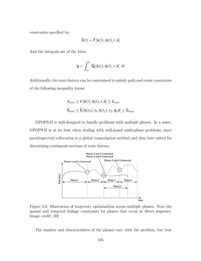
constraints specified by:

˙x(t) = f [x(t), u(t), t, s]

And the integrals are of the form:

q =

∫ tf

t0

Q [x(t), u(t), t, s] dt

Additionally, the state history can be constrained to satisfy path and event constraints

of the following inequality forms:

cmin ≤ c [x(t), u(t), t, s] ≤ cmax

bmin ≤ b [x(t0), t0, x(tf ), tf , q, s] ≤ bmax

GPOPS-II is well-designed to handle problems with multiple phases. In a sense,

GPOPS-II is at its best when dealing with well-posed multi-phase problems, since

pseudospectral collocation is a global transcription method and thus best suited for

discretizing continuous sections of state history.

Phase 1 Phase 2 Phase 3

Phase 5

Phase 4

Tra

ject

ory

time

Phases 1 and 2 Connected

Phases 2 and 3 ConnectedPhases 2 and 5 Connected

Phases 3 and 4 Connected

Figure 3.2: Illustration of trajectory optimization across multiple phases. Note thespatial and temporal linkage constraints for phases that occur in direct sequence.Image credit: [30]

The number and characteristics of the phases vary with the problem, but best

105

practice is to implement them when there is are natural discontinuities in certain

aspects of the problem. For example, dynamics may change for the system at a certain

time, such as for a staged ascent vehicle. If it is known that control discontinuities

feature in the optimal solution, phases should be implemented for each section of

continuous control, such as in the minimum-fuel satellite maneuver problem where it

is advantageous to allow three phases to accommodate the three sections of the ‘bang-

off-bang’ solution. Most relevantly to this thesis, long-duration proximity operations

can be separated into sections where path constraints are or are not enforced, which

is useful for encoding trajectories that feature zero-thrust circumnavigation periods.

The usefulness of this capability to handle phases is that the phase boundary times

need not be known a priori. Guidelines for the implementation of phases in GPOPS-

II are given by Rao [30], and include (at a minimum) linkage logic for constraining

temporal and spatial endpoints of the phases. Sets of more stringent phase linkage

constraints are later leveraged as tools for analyzing proximity operations trajectories

with free-orbit phases.

3.3.2 Implementation Approach

GPOPS-II requires compliance with a specific set of function interactions in MAT-

LAB. At the very least, there needs to be a ‘Main’ function, a ‘Continuous’ function,

and an ‘Endpoint’ function. This subsection describes how the Rendezvous / Proxim-

ity Operations Trajectory Analysis Tool (R/POTATO), one of the main contributions

of this thesis, was implemented by adding an instantiation shell and modifying ‘Main,’

‘Continuous,’ and ‘Endpoint’ to comply with pervasive problem formulation flags.

106

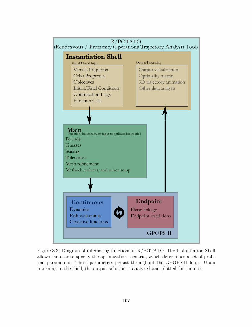
Instantiation Shell

Output visualizationOptimality metric 3D trajectory animationOther data analysis

Main

ContinuousDynamicsPath constraintsObjective functions

EndpointPhase linkageEndpoint conditions

BoundsGuessesScalingTolerancesMesh refinementMethods, solvers, and other setup

GPOPS-II

R/POTATO (Rendezvous / Proximity Operations Trajectory Analysis Tool)

Function that constructs input to optimization routine

Vehicle PropertiesOrbit PropertiesObjectivesInitial/Final ConditionsOptimization FlagsFunction Calls

User-Defined Input Output Processing

Figure 3.3: Diagram of interacting functions in R/POTATO. The Instantiation Shellallows the user to specify the optimization scenario, which determines a set of prob-lem parameters. These parameters persist throughout the GPOPS-II loop. Uponreturning to the shell, the output solution is analyzed and plotted for the user.

107

3.3.2.1 Instantiation Shell

This function was created to collect a variety of the ways that the proximity oper-

ations problem can be instantiated into one place, as well as to unpack and visualize

the data from the returned solution after the GPOPS-II optimization loop terminates.

The most basic function that the shell performs is to supply initial conditions and

problem parameters such as vehicle mass, inertia, thruster type, saturation limits,

orbit altitude, and thruster geometry to the solver.

Various flags can be set in the user-modifiable section of the instantiation shell.

Based on which flags are set, GPOPS-II will instantiate the problem in different ways

based on logical checks contained in ‘Main,’ ‘Continuous,’ and ‘Endpoint.’ The table

in Appendix D summarizes the effect of each flag. The intent is not to exhaust the

possible ways that a proximity operations problem can be specified, but rather to

demonstrate a variety of interesting ways to pose the problem that leverages the

generality of GPOPS-II’s optimization method.

An additional feature of the Instantiation Shell is the back-computation of the

problem’s Hamiltonian as a function of time using the solution structure. GPOPS-II

cannot provide an exact optimal solution because it optimizes over a finite discretiza-

tion of the problem to the specified tolerance and mesh refinement; for this reason, it

is useful to have an optimality metric for the returned solution. It can be shown with

the variational approach to the optimal control problem that if the cost integrand g

and the state dynamics f are not explicit functions of time, then the Hamiltonian is

at least piecewise constant [25]:

H = g(x, u) + pT f(x, u)

Where p is the costate. Furthermore, problems without a fixed final time (such as the

108

minimum time optimization) where the endpoint condition is not explicitly a function

of time should cause the H = 0 for all time by the transversality condition.

The Instantiation Shell obtains the state and costate histories from the GPOPS-

II solution structure and computes the Hamiltonian history as an optimality metric.

Near-optimal minimum-time problems should have very small Hamiltonian values.

Near-optimal minimum-energy problems should have nearly constant, but non-zero,

Hamilton values. Problems with multiple phases or control discontinuities should

have a piecewise-constant Hamiltonian. This same metric is also used by Boyarko, et

al. [6] to observe the optimality of their solver solution outputs.

3.3.2.2 Main

‘Main’ is part of the GPOPS-II function dependency structure. Several examples

of Main functions are provided in the form of example problems that are included

with the download of GPOPS-II. Its purpose is to provide bounds and guesses for

the problem variables: time, states, controls, integrals, constraints, and event groups.

The initial and final values of the time and states are also specified here. Problem

parameters created in the Instantiation Shell are encoded as auxiliary data by Main,

which is a data structure that is visible to Continuous and Endpoint and persists

throughout the optimization loop.

Additionally, mesh refinement and collocation parameters, mesh tolerance, as well

as scaling and differentiation methods are set here. In all cases, hp mesh adaptation

appears to yield fast and accurate results. Mesh refinement and tolerance parameters

should be set to achieve the desired balance of precision and computation time, which

can vary with the problem being solved. Automatic differentiation techniques, such

as provided by Adigator, are ill-suited to dealing with the modified structure of Con-

tinuous and Endpoint, so the built-in ‘sparseCD’ method is used instead. Problem

109

scaling determined automatically from the variable bounds can be a good starting

point for timely computation, but was found to be detrimental to solution quality in

certain cases. As mentioned previously, IPOPT [39] was chosen as the NLP solver.

3.3.2.3 Continuous

‘Continuous’ receives the auxiliary data structure from ‘Main’ and computes state

dynamics, path constraint values, and objective function values for the problem.

Thus, operations on the time, state, and control variables must be implemented

here. Although many computations would be compactly performed with matrix or

quaternion multiplication on groups of state variables, this is not straightforward to

implement in Continuous; realize that these computations are actually performed on

a given iteration’s vector of collocation points, so all matrix products are written

out as scalar expressions with element-by-element computations on a given variable’s

collocation vector.

If a problem is instantiated with eccentricity in the reference orbit, the Keplerian

state dynamics are a function of the target’s true anomaly (see Chapter 2). Because

the determination of true anomaly from time-of-flight (Kepler’s Problem) has no

closed-form solution and requires its own numerical root-finding techniques, a true

anomaly look-up table is pre-computed by the Instantiation Shell before being passed

to Continuous, which interpolates true anomalies for the current iteration’s vector of

collocation points based on their time fields. This way, it is not necessary to repeatedly

solve Kepler’s Problem, which substantially speeds up computation.

3.3.2.4 Endpoint

‘Endpoint,’ like ‘Continuous,’ is called with every mesh iteration. It also receives

the auxiliary data structure from Main, which determines what sections of Endpoint

110

are run to achieve the desired problem phasing with appropriate endpoint linkage

constraints. As was the case in Continuous, operations on time, state, and control

variables must be performed as element-wise scalar operations on the current itera-

tion’s collocation vectors.

If the user-defined parameters indicate the desire for a free-orbit (zero-thrust pe-

riodic) phase, a set of linkage constraints are implemented as conditions for entering

the phase (for example, the period-matching constraint, along with any other size

and orientation specifications). Treating the free-orbit trajectory as a dynamics rep-

resents a more sophisticated approach for phasing into a free-orbit trajectory than

simply choosing a pre-determined location in the state space as an entry-point for the

trajectory. The resultant effect of not specifying the trajectory entry-point a priori

on problem optimality is visualized in Figure 3.4.

111

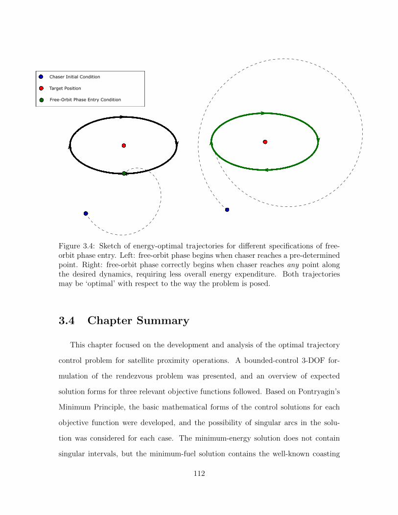
Chaser Initial Condition

Target Position

Free-Orbit Phase Entry Condition

Figure 3.4: Sketch of energy-optimal trajectories for different specifications of free-orbit phase entry. Left: free-orbit phase begins when chaser reaches a pre-determinedpoint. Right: free-orbit phase correctly begins when chaser reaches any point alongthe desired dynamics, requiring less overall energy expenditure. Both trajectoriesmay be ‘optimal’ with respect to the way the problem is posed.

3.4 Chapter Summary

This chapter focused on the development and analysis of the optimal trajectory

control problem for satellite proximity operations. A bounded-control 3-DOF for-

mulation of the rendezvous problem was presented, and an overview of expected

solution forms for three relevant objective functions followed. Based on Pontryagin’s

Minimum Principle, the basic mathematical forms of the control solutions for each

objective function were developed, and the possibility of singular arcs in the solu-

tion was considered for each case. The minimum-energy solution does not contain

singular intervals, but the minimum-fuel solution contains the well-known coasting

112

interval as part of its ‘bang-off-bang’ control. Most surprisingly, the minimum-time

problem admits the possibility of a degenerate class of singular solutions even with

LTI dynamics due to the MIMO formulation of the problem, which is best described

as ‘scheduling ambiguity.’

The issue of scheduling ambiguity in the minimum-time problem motivated the

exploration of techniques to resolve it. The simplest technique is to adopt a scheduling

policy, which collapses the singular class to a unique solution. This works well due

to the separable nature of the Clohessy-Wiltshire dynamics for in-plane versus out-

of-plane motion. A more sophisticated approach leveraging this separability was also

presented in the form of a hybrid time-energy-optimal solution, where non-limiting

coordinates are optimized for energy use instead of extremal state regulation, which

is equally time-optimal to the scheduling policy solution but uses considerably less

fuel.

The third mitigation strategy is to couple position and attitude dynamics. If

the bounded control is taken to be a physical limitation on propulsion devices, then

this is the most physically consistent formulation of the optimal proximity operations

problem. A single-thruster bounded-control 6-DOF formulation using a quaternion

representation of attitude was presented with 13 states and 4 control variables. The

unique time-optimal rendezvous solution in this formulation corroborates the intuitive

‘straight-line’ approach trajectory, which is actually faster than the frame-saturated

3-DOF result for the same initial conditions.

Situations where translational acceleration inputs can be generalized into frame

coordinate inputs (i.e. uncoupled with attitude via real-time thrust mixing) were

determined to be the relatively low-thrust, long-time-horizon minimum-energy prob-

lems. The ability to uncouple translation and rotation is exceedingly useful because

the search space for the 3-DOF formulation is much more manageable for practi-

113

cal computational resources than that for the 6-DOF formulation. For this reason,

continuous-thrust, minimum-energy trajectories will be the main focus of the anal-

ysis in the chapter to follow of extended proximity operations under higher-fidelity

dynamics and various path constraints.

The Rendezvous / Proximity Operations Trajectory Analysis Tool (R/POTATO),

a MATLAB framework that implements numerical trajectory optimization provided

by GPOPS-II [30], was introduced as a contribution of this thesis. The numerical

optimization method used by GPOPS-II was found to be well-suited to the optimal

proximity operations problem, as it performs multi-phase pseudospectral collocation

which admits very general formulations of optimization problems.

The chapter to follow examines results that validate the numerical optimization

framework using the MIMO state regulation problem formulations presented in this

chapter. It then builds on these preliminary results by combining the orbit mechanical

discussion of long-duration proximity operations from Chapter 2 with the numerical

optimization capabilities of GPOPS-II and R/POTATO described and validated in

this chapter.

114

Chapter 4

Results

In Chapter 2, the orbital mechanics of long-duration proximity operations were an-

alyzed in the perturbation-free Keplerian dynamics as well as the linearized Clohessy-

Wiltshire dynamics, and it was found that the assumptions which linearize spherical

gravity are most valid for proximity operations which are near to the target and occur

on short timescales – in effect, operations in their ‘terminal phase’ of the trajectory,

a phrase which features in Clohessy and Wiltshire’s original publication [10]. Lin-

earization error grew when the chaser spent prolonged periods at a distance from the

target, as well as when the eccentricity of the target orbit was given a realistic value.

By its nature, the conduct of prolonged proximity operations is more prone to the

accumulation of this linearization error than docking maneuvers.

In Chapter 3, the optimal trajectory control problem was introduced and ana-

lyzed. The MIMO state regulation problem with LTI dynamics proved to be the

most straightforward to analyze mathematically, but it was found that degenerate

sub-optimal solution classes exist for objectives requiring extremal control in the

case where the control inputs appear linearly in the acceleration model and saturate

independently (frame-component saturation). This motivated the development of

coupled position-and-attitude dynamics, which remove the ambiguity from extremal

control cases; however, it was determined that sufficiently reachable minimum-energy

115

problems can avoid the consideration of coupling attitude dynamics (e.g., by using a

thruster selection technique to apply frame-component acceleration inputs).

A numerical optimization framework tailored for the analysis of proximity opera-

tions trajectories was also presented in Chapter 3. The framework is flexible enough

to use either linear and nonlinear dynamics, allowing the analysis of trajectories with

higher-fidelity acceleration models. The problem can also be implemented with as

many states and inputs as desired, allowing for the analysis of attitude-coupled ma-

neuvers with a variety of thruster geometries. Finally, arbitrarily complex endpoint

conditions and path constraints can be implemented over various phases of the prob-

lem. Each of these prove to be useful characteristics for analyzing long-duration

proximity operations.

This chapter presents the results of the implementation of various proximity oper-

ations scenarios in the Rendezvous / Proximity Operations Trajectory Analysis Tool.

Because there are a large number of scenarios that can be analyzed by setting various

combinations of flags in the Instantiation Shell, only certain demonstrative scenarios

are analyzed according to the approach described in the section below.

4.1 Approach to Results Chapter

This chapter comprises three main sections. The first will focus on the valida-

tion of the solution produced by GPOPS-II when supplied with the relatively sim-

ple minimum-energy, minimum-time, and minimum-fuel MIMO rendezvous objective

with LTI dynamics, for which the solution form is well-known. The second main

section will expand the analysis to explore solutions to problems which require more

complicated formulation, such as the implementation of path constraints, nonlinear

dynamics, or coupling attitude dynamics. The third main section will shift the focus

116

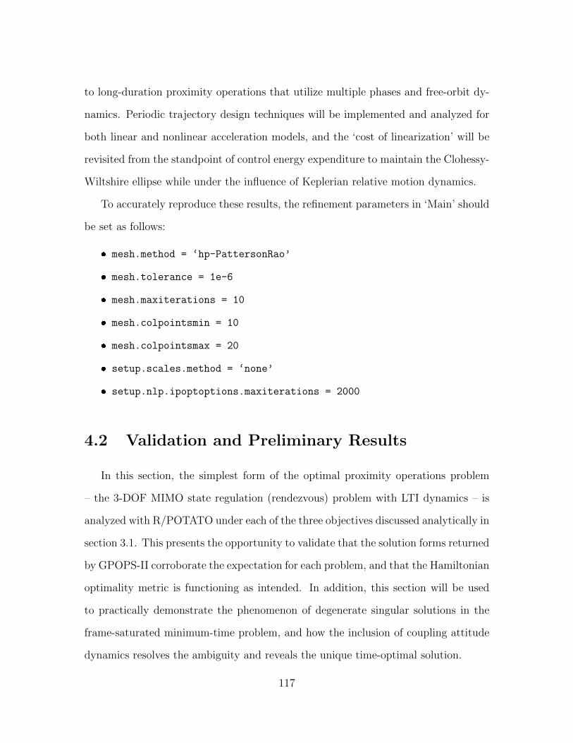
to long-duration proximity operations that utilize multiple phases and free-orbit dy-

namics. Periodic trajectory design techniques will be implemented and analyzed for

both linear and nonlinear acceleration models, and the ‘cost of linearization’ will be

revisited from the standpoint of control energy expenditure to maintain the Clohessy-

Wiltshire ellipse while under the influence of Keplerian relative motion dynamics.

To accurately reproduce these results, the refinement parameters in ‘Main’ should

be set as follows:

mesh.method = ‘hp-PattersonRao’

mesh.tolerance = 1e-6

mesh.maxiterations = 10

mesh.colpointsmin = 10

mesh.colpointsmax = 20

setup.scales.method = ‘none’

setup.nlp.ipoptoptions.maxiterations = 2000

4.2 Validation and Preliminary Results

In this section, the simplest form of the optimal proximity operations problem

– the 3-DOF MIMO state regulation (rendezvous) problem with LTI dynamics – is

analyzed with R/POTATO under each of the three objectives discussed analytically in

section 3.1. This presents the opportunity to validate that the solution forms returned

by GPOPS-II corroborate the expectation for each problem, and that the Hamiltonian

optimality metric is functioning as intended. In addition, this section will be used

to practically demonstrate the phenomenon of degenerate singular solutions in the

frame-saturated minimum-time problem, and how the inclusion of coupling attitude

dynamics resolves the ambiguity and reveals the unique time-optimal solution.

117

4.2.1 Linear Quadratic Regulator

One way to validate R/POTATO is to formulate an optimal control problem for

which a closed-form analytical solution is easily obtainable. One such formulation is

the linear quadratic regulator, where the objective is to minimize the cost function:

J =

∫ tf

t0

1

2

[xTQx + uTRu

]With tf = 86, 400 s. It is known that optimal control law for the infinite-time-

horizon LQR problem takes the form:

u∗(t) = −Kx(t)

Where the LQR gain K can be obtained as the solution to an algebraic Ricatti

equation if the state dynamics are linear and time-invariant. The infinite-horizon

control solution approximates the finite-time solution in this case, because the plant

is completely controllable and the linearized Clohessy-Wiltshire relative dynamics are

LTI [25]. Thus, the result from R/POTATO can be directly compared to a simulated

full-state feedback trajectory with the LQR gain determined algebraically from the

same parameters. To obtain this result, mesh tolerance was reduced to 1e-9 and

Quadratic_Cost was set to 1 with Q_R_ratio = 1e-10. The initial condition used

ensures that motion in every coordinate must be regulated:

x0 = [100m 110m 250m 0.1m/s 0.1m/s 0.1m/s]T

118

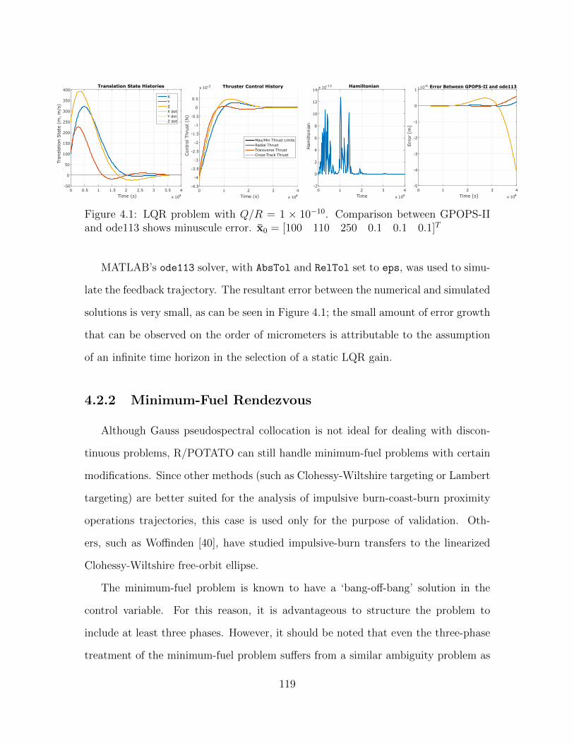
0 0.5 1 1.5 2 2.5 3 3.5 4

Time (s) x 104

-50

0

50

100

150

200

250

300

350

400

Tran

slat

ion S

tate

(m

, m

/s)

Translation State Histories

XYZX dotY dotZ dot

0 1 2 3 4

Time (s) x 104

-4.5

-4

-3.5

-3

-2.5

-2

-1.5

-1

-0.5

0

0.5

Con

trol

Thru

st (

N)

x 10-3 Thruster Control History

Max/Min Thrust LimitsRadial ThrustTransverse ThrustCross-Track Thrust

0 1 2 3 4

Time x 104

-2

0

2

4

6

8

10

12

14

Ham

ilton

ian

x 10-13 Hamiltonian

0 1 2 3 4

Time [s] x 104

-5

-4

-3

-2

-1

0

1

Err

or

[m]

x10-6 Error Between GPOPS-II and ode113

Figure 4.1: LQR problem with Q/R = 1 × 10−10. Comparison between GPOPS-IIand ode113 shows minuscule error. x0 = [100 110 250 0.1 0.1 0.1]T

MATLAB’s ode113 solver, with AbsTol and RelTol set to eps, was used to simu-

late the feedback trajectory. The resultant error between the numerical and simulated

solutions is very small, as can be seen in Figure 4.1; the small amount of error growth

that can be observed on the order of micrometers is attributable to the assumption

of an infinite time horizon in the selection of a static LQR gain.

4.2.2 Minimum-Fuel Rendezvous

Although Gauss pseudospectral collocation is not ideal for dealing with discon-

tinuous problems, R/POTATO can still handle minimum-fuel problems with certain

modifications. Since other methods (such as Clohessy-Wiltshire targeting or Lambert

targeting) are better suited for the analysis of impulsive burn-coast-burn proximity

operations trajectories, this case is used only for the purpose of validation. Oth-

ers, such as Woffinden [40], have studied impulsive-burn transfers to the linearized

Clohessy-Wiltshire free-orbit ellipse.

The minimum-fuel problem is known to have a ‘bang-off-bang’ solution in the

control variable. For this reason, it is advantageous to structure the problem to

include at least three phases. However, it should be noted that even the three-phase

treatment of the minimum-fuel problem suffers from a similar ambiguity problem as

119

the minimum-time problem: the first ‘bang’ phase will be as long as required for

the limiting coordinate’s pulse, but pulses for the non-limiting coordinates need not

last the entire length of the phase. Essentially, the solver struggles when the optimal

control trajectory on a given phase includes both extremal and null control, so it can

be difficult to structure the problem with phase boundaries that are robust.

For simple validation and to avoid scheduling ambiguity, the chaser’s initial con-

dition will be set as follows:

x0 = [0m −5000m 0m 0m/s 0m/s 0m/s]T

This initial condition represents the linearized ‘string-of-pearls’ scenario, where

the chaser is initially 5 kilometers behind the target (but is assumed to be along the

target’s orbital trajectory). The single-period minimum-fuel strategy for the chaser

is to apply two burns (as impulsively as possible), one which lowers perigee to phase

forward in the direction of the target, and the other which circularizes near the

terminus. This is also known as Hohmann phasing.

From basic orbital mechanics, one can calculate the magnitude of each burn’s

symmetrical ∆V:

Vtgt = (42 164 137m)(7.29212× 10−5rev/s) = 3 074.661m/s

∆T =5 000m

3 074.661m/s= 1.626s

Tphasing = Ttgt −∆T = 86162.364s ∴ aphasing = 42 163 606.48m

∆V = Vtgt − Vphasingapo = 3 074.661m/s−√µ

(2

atgt− 1

aphasing

)= 0.01934 m/s

To pose this problem to R/POTATO, set the above initial conditions along with

120

the following flags in the Instantiation Shell:

Incl_Att_Dynamics = 0

Min_Fuel = 1

Three_Phase = 1

Bang_Width = 10

Target_Point = 1

Nonlinear = 0

Max_Time = 86400

HallEffectThrust = 1

It greatly alleviates computation time to manually fix the control bounds to max-

imum or minimum thrust for the duration of the initial and terminal phases of the

problem, and to fix the control bounds at zero for the coasting phase. This tech-

nique leverages the known solution form of the minimum-fuel trajectory to reduce

the problem to a simple burn-time optimization problem for the solver. This is more

easily done with simpler optimization tools, and for this reason, R/POTATO is not

recommended for use on the minimum-fuel problem. The result is shown below:

121

1 2 3 4 5 6 7

Time (s)

-0.06

-0.05

-0.04

-0.03

-0.02

-0.01

0

0.01

0.02

0.03

Tran

slat

ion S

tate

(m

, m

/s)

Translation State Histories (Phase 1)

XYZX dotY dotZ dot

X: 3.872Y: -0.01936

0 1 2 3 4 5

Time (s)

-0.5

-0.4

-0.3

-0.2

-0.1

0

0.1

0.2

0.3

0.4

0.5

Con

trol

Thru

st (

N)

Control History (Phase 1)

0 2 4

Time

-0.9975

-0.997

-0.9965

-0.996

-0.9955

-0.995

-0.9945

-0.994

-0.9935

Ham

ilton

ian

Hamiltonian (Phase 1)

8.63958.63968.63978.63988.6399 8.64

Time (s) x 104

-0.5

-0.4

-0.3

-0.2

-0.1

0

0.1

0.2

0.3

0.4

0.5

Control History (Phase 3)

8.6396 8.6398 8.64

Time x 104

0.996

0.997

0.998

0.999

1

1.001

1.002

1.003

1.004

Hamiltonian (Phase 3)

0 1 2 3 4 5 6 7 8

Time (s) x 104

-6000

-5000

-4000

-3000

-2000

-1000

0

1000

Tran

slat

ion S

tate

(m

, m

/s)

Translation State Histories

XYZX dotY dotZ dot

Transverse Thrust

Phase Separation Marker

Max/Min Thrust LimitsRadial Thrust

Cross-Track Thrust

Figure 4.2: 6-Thruster Min-Time w/ Attitude: x0 = [10 11 25 0.1 0.1 0.1]T

It can be seen from the state history that the expected phasing trajectory is the

minimum-fuel result. The solver determined that the required on-time for the thruster

was 3.872 seconds, which produces a ∆V of 0.01936 m/s - only slightly more than

was calculated above, likely because a small amount less than a sidereal day was

allotted for the maneuver. The result from this minimum-fuel problem shows that

R/POTATO returns the expected trajectory with about the same ∆V that can easily

be calculated from orbit mechanical equations. The total amount of fuel used for this

trajectory was 7.744 normalized fuel units (calculated as the integral sum of control

variable magnitudes, and abbreviated NFU from this point forward. Multiplying this

value by the maximum thrust force yields the total impulse of the maneuver in N·s).

122

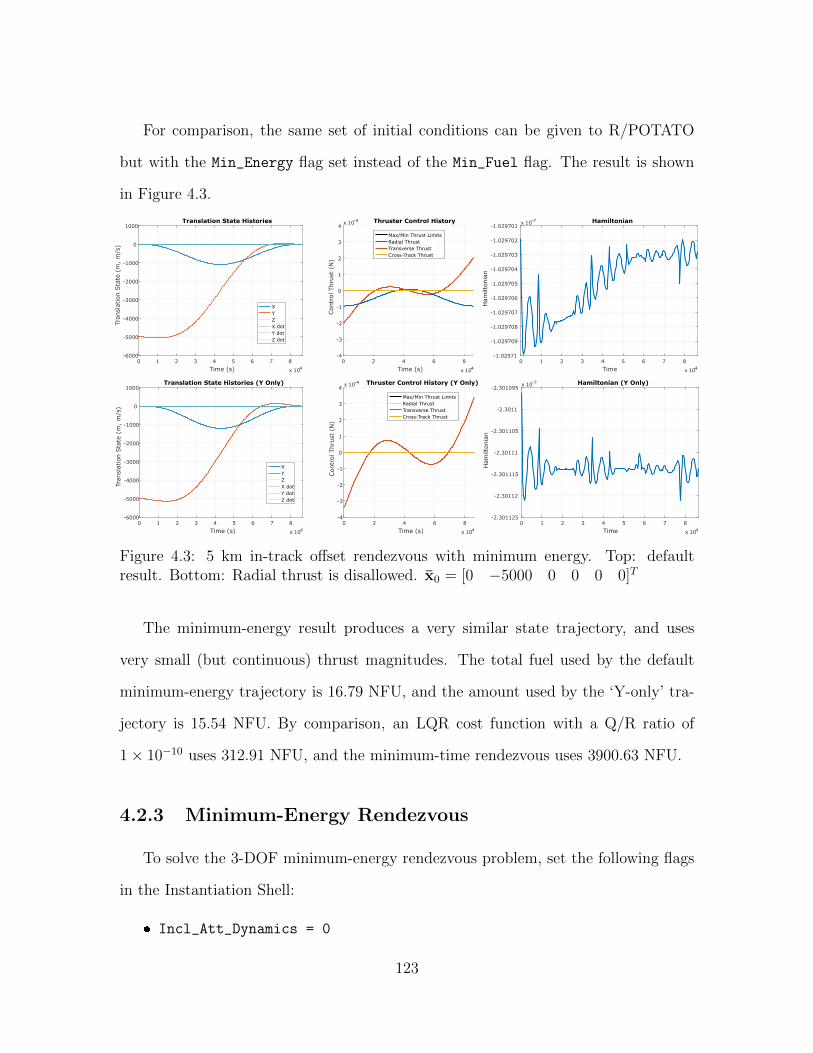
For comparison, the same set of initial conditions can be given to R/POTATO

but with the Min_Energy flag set instead of the Min_Fuel flag. The result is shown

in Figure 4.3.

0 1 2 3 4 5 6 7 8

Time (s) x 104

-6000

-5000

-4000

-3000

-2000

-1000

0

1000

Tran

slat

ion S

tate

(m

, m

/s)

Translation State Histories

XYZX dotY dotZ dot

0 2 4 6 8

Time (s) x 104

-4

-3

-2

-1

0

1

2

3

4

Con

trol

Thru

st (

N)

x 10-4 Thruster Control History

Max/Min Thrust LimitsRadial ThrustTransverse ThrustCross-Track Thrust

0 1 2 3 4 5 6 7 8

Time x 104

-1.02971

-1.029709

-1.029708

-1.029707

-1.029706

-1.029705

-1.029704

-1.029703

-1.029702

-1.029701

Ham

ilton

ian

x 10-7 Hamiltonian

0 1 2 3 4 5 6 7 8

Time (s) x 104

-6000

-5000

-4000

-3000

-2000

-1000

0

1000

Tran

slat

ion S

tate

(m

, m

/s)

Translation State Histories (Y Only)

XYZX dotY dotZ dot

0 2 4 6 8

Time (s) x 104

-4

-3

-2

-1

0

1

2

3

4

Con

trol

Thru

st (

N)

x 10-4 Thruster Control History (Y Only)

Max/Min Thrust LimitsRadial ThrustTransverse ThrustCross-Track Thrust

0 1 2 3 4 5 6 7 8

Time x 104

-2.301125

-2.30112

-2.301115

-2.30111

-2.301105

-2.3011

-2.301095

Ham

ilton

ian

x 10-7 Hamiltonian (Y Only)

Figure 4.3: 5 km in-track offset rendezvous with minimum energy. Top: defaultresult. Bottom: Radial thrust is disallowed. x0 = [0 −5000 0 0 0 0]T

The minimum-energy result produces a very similar state trajectory, and uses

very small (but continuous) thrust magnitudes. The total fuel used by the default

minimum-energy trajectory is 16.79 NFU, and the amount used by the ‘Y-only’ tra-

jectory is 15.54 NFU. By comparison, an LQR cost function with a Q/R ratio of

1× 10−10 uses 312.91 NFU, and the minimum-time rendezvous uses 3900.63 NFU.

4.2.3 Minimum-Energy Rendezvous

To solve the 3-DOF minimum-energy rendezvous problem, set the following flags

in the Instantiation Shell:

Incl_Att_Dynamics = 0

123

Min_Energy = 1

Target_Point = 1

Nonlinear = 0

HallEffectThrust = 1

GEO = 1

It was shown in Section 3.1 that the solution to the minimum-energy rendezvous

problem consists of sinusoid sections in the control wherever permissible. Also, the

Hamiltonian should be constant for all time while on a truly energy-optimal trajectory.

The result of implementation in R/POTATO is shown in Figures 4.4 and 4.5 below.

GPOPS-II’s pseudospectral collocation method is very well-suited to this problem in

particular due to the smoothness of the state and control trajectories; the problem

can be solved in seconds to the specified mesh tolerance.

0 2 4 6 8

Time (s) #104

-6000

-5000

-4000

-3000

-2000

-1000

0

1000

2000

Tran

slat

ion S

tate

(m

, m

/s)

Translation State Histories

XYZX dotY dotZ dot

0 2 4 6 8

Time (s) x 104

-1.5

-1

-0.5

0

0.5

1

Con

trol

Thru

st (

N)

#10-3 Thruster Control History

Max/Min Thrust LimitsRadial ThrustTransverse ThrustCross-Track Thrust

0 2 4 6 8

Time x 104

-1.0491576

-1.0491574

-1.0491572

-1.049157

-1.0491568

-1.0491566

-1.0491564

-1.0491562

-1.049156

-1.0491558

-1.0491556

Ham

ilton

ian

x 10-6 Hamiltonian

Figure 4.4: Minimum Energy: 24 hours, Hall effect thruster, with initial condition:[100, 110, 250, 0.1, 0.1, 0.1]

124

-2000

-1000

0

1000

2000

3000

4000

Rad

ial [m

]

-6000-5000-4000-3000-2000-10000

In-Track [m]

24-hr HET Min-Energy: Orbital Plane Trajectory

Optimal Rendezvous TrajectoryInitial PositionFinal PositionUnforced Trajectory

Figure 4.5: Minimum-energy trajectory in the orbital plane. Thrust is graduallyapplied to achieve the rendezvous trajectory that is the ‘path of least resistance’ tonatural motion in a 24-hour time limit.

These results indicate control histories which are sinusoid sections and a Hamil-

tonian which is very nearly constant. This corroborates the expectation for the

minimum-energy solution. The minimum-time and minimum-fuel problems are less

straightforward to analyze with this tool, however.

4.2.4 Minimum-Time Rendezvous

To solve the minimum-time problem without any strategy to mitigate scheduling

ambiguity, set the following flags in the Instantiation Shell:

Incl_Att_Dynamics = 0

Min_Time = 1

Sched_Pol = 0

Hybrid_Opt = 0

Target_Point = 1

Nonlinear = 0

125

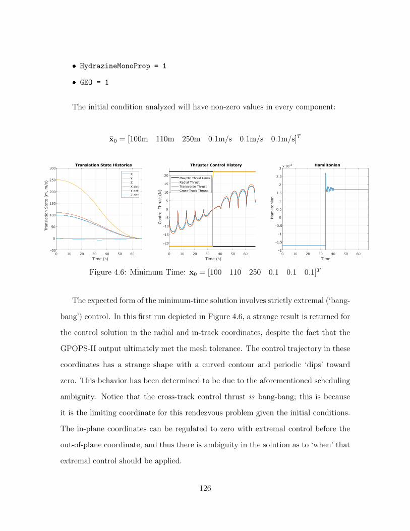
HydrazineMonoProp = 1

GEO = 1

The initial condition analyzed will have non-zero values in every component:

x0 = [100m 110m 250m 0.1m/s 0.1m/s 0.1m/s]T

0 10 20 30 40 50 60

Time (s)

-50

0

50

100

150

200

250

300

Tran

slat

ion S

tate

(m

, m

/s)

Translation State Histories

XYZX dotY dotZ dot

0 10 20 30 40 50 60

Time (s)

-20

-15

-10

-5

0

5

10

15

20

Con

trol

Thru

st (

N)

Thruster Control History

Max/Min Thrust Limits

Radial ThrustTransverse ThrustCross-Track Thrust

0 10 20 30 40 50 60

Time

-2

-1.5

-1

-0.5

0

0.5

1

1.5

2

2.5

3

Ham

ilton

ian

x 10-3 Hamiltonian

Figure 4.6: Minimum Time: x0 = [100 110 250 0.1 0.1 0.1]T

The expected form of the minimum-time solution involves strictly extremal (‘bang-

bang’) control. In this first run depicted in Figure 4.6, a strange result is returned for

the control solution in the radial and in-track coordinates, despite the fact that the

GPOPS-II output ultimately met the mesh tolerance. The control trajectory in these

coordinates has a strange shape with a curved contour and periodic ‘dips’ toward

zero. This behavior has been determined to be due to the aforementioned scheduling

ambiguity. Notice that the cross-track control thrust is bang-bang; this is because

it is the limiting coordinate for this rendezvous problem given the initial conditions.

The in-plane coordinates can be regulated to zero with extremal control before the

out-of-plane coordinate, and thus there is ambiguity in the solution as to ‘when’ that

extremal control should be applied.

126

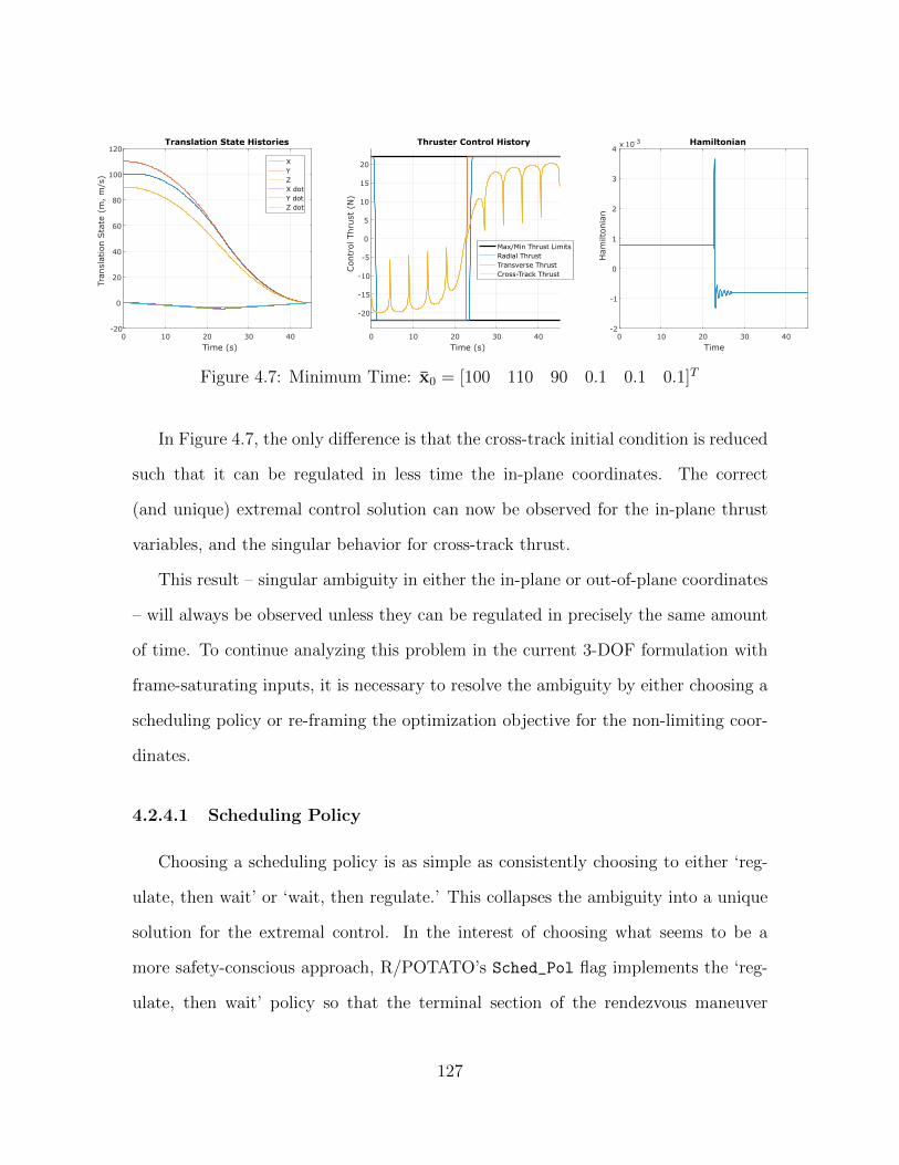
0 10 20 30 40

Time (s)

-20

0

20

40

60

80

100

120

Tran

slat

ion S

tate

(m

, m

/s)

Translation State Histories

XYZX dotY dotZ dot

0 10 20 30 40

Time (s)

-20

-15

-10

-5

0

5

10

15

20

Con

trol

Thru

st (

N)

Thruster Control History

Max/Min Thrust LimitsRadial ThrustTransverse ThrustCross-Track Thrust

0 10 20 30 40

Time

-2

-1

0

1

2

3

4

Ham

ilton

ian

x 10-3 Hamiltonian

Figure 4.7: Minimum Time: x0 = [100 110 90 0.1 0.1 0.1]T

In Figure 4.7, the only difference is that the cross-track initial condition is reduced

such that it can be regulated in less time the in-plane coordinates. The correct

(and unique) extremal control solution can now be observed for the in-plane thrust

variables, and the singular behavior for cross-track thrust.

This result – singular ambiguity in either the in-plane or out-of-plane coordinates

– will always be observed unless they can be regulated in precisely the same amount

of time. To continue analyzing this problem in the current 3-DOF formulation with

frame-saturating inputs, it is necessary to resolve the ambiguity by either choosing a

scheduling policy or re-framing the optimization objective for the non-limiting coor-

dinates.

4.2.4.1 Scheduling Policy

Choosing a scheduling policy is as simple as consistently choosing to either ‘reg-

ulate, then wait’ or ‘wait, then regulate.’ This collapses the ambiguity into a unique

solution for the extremal control. In the interest of choosing what seems to be a

more safety-conscious approach, R/POTATO’s Sched_Pol flag implements the ‘reg-

ulate, then wait’ policy so that the terminal section of the rendezvous maneuver

127

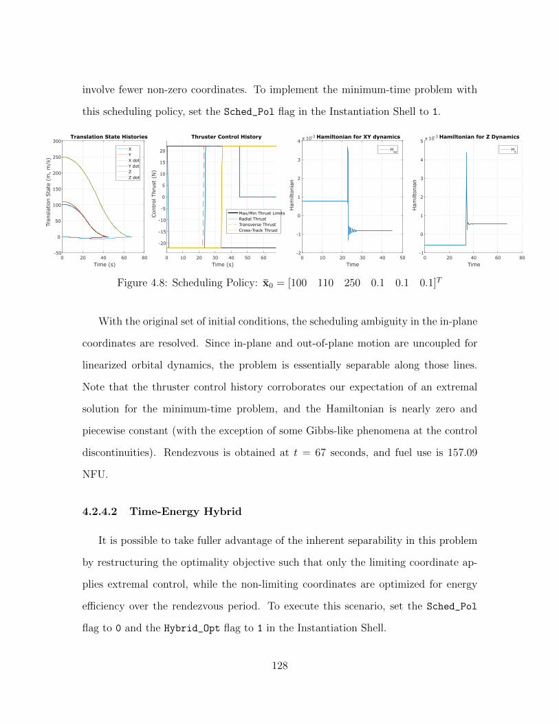
involve fewer non-zero coordinates. To implement the minimum-time problem with

this scheduling policy, set the Sched_Pol flag in the Instantiation Shell to 1.

0 20 40 60 80

Time (s)

-50

0

50

100

150

200

250

300

Tran

slat

ion S

tate

(m

, m

/s)

Translation State Histories

XYX dotY dotZZ dot

0 10 20 30 40 50 60

Time (s)

-20

-15

-10

-5

0

5

10

15

20Con

trol

Thru

st (

N)

Thruster Control History

Max/Min Thrust LimitsRadial ThrustTransverse ThrustCross-Track Thrust

0 10 20 30 40 50

Time

-2

-1

0

1

2

3

4

Ham

ilton

ian

x 10-3 Hamiltonian for XY dynamics

Hxy

0 20 40 60 80

Time

-1

0

1

2

3

4

5

Ham

ilton

ian

x 10-3 Hamiltonian for Z Dynamics

Hz

Figure 4.8: Scheduling Policy: x0 = [100 110 250 0.1 0.1 0.1]T

With the original set of initial conditions, the scheduling ambiguity in the in-plane

coordinates are resolved. Since in-plane and out-of-plane motion are uncoupled for

linearized orbital dynamics, the problem is essentially separable along those lines.

Note that the thruster control history corroborates our expectation of an extremal

solution for the minimum-time problem, and the Hamiltonian is nearly zero and

piecewise constant (with the exception of some Gibbs-like phenomena at the control

discontinuities). Rendezvous is obtained at t = 67 seconds, and fuel use is 157.09

NFU.

4.2.4.2 Time-Energy Hybrid

It is possible to take fuller advantage of the inherent separability in this problem

by restructuring the optimality objective such that only the limiting coordinate ap-

plies extremal control, while the non-limiting coordinates are optimized for energy

efficiency over the rendezvous period. To execute this scenario, set the Sched_Pol

flag to 0 and the Hybrid_Opt flag to 1 in the Instantiation Shell.

128

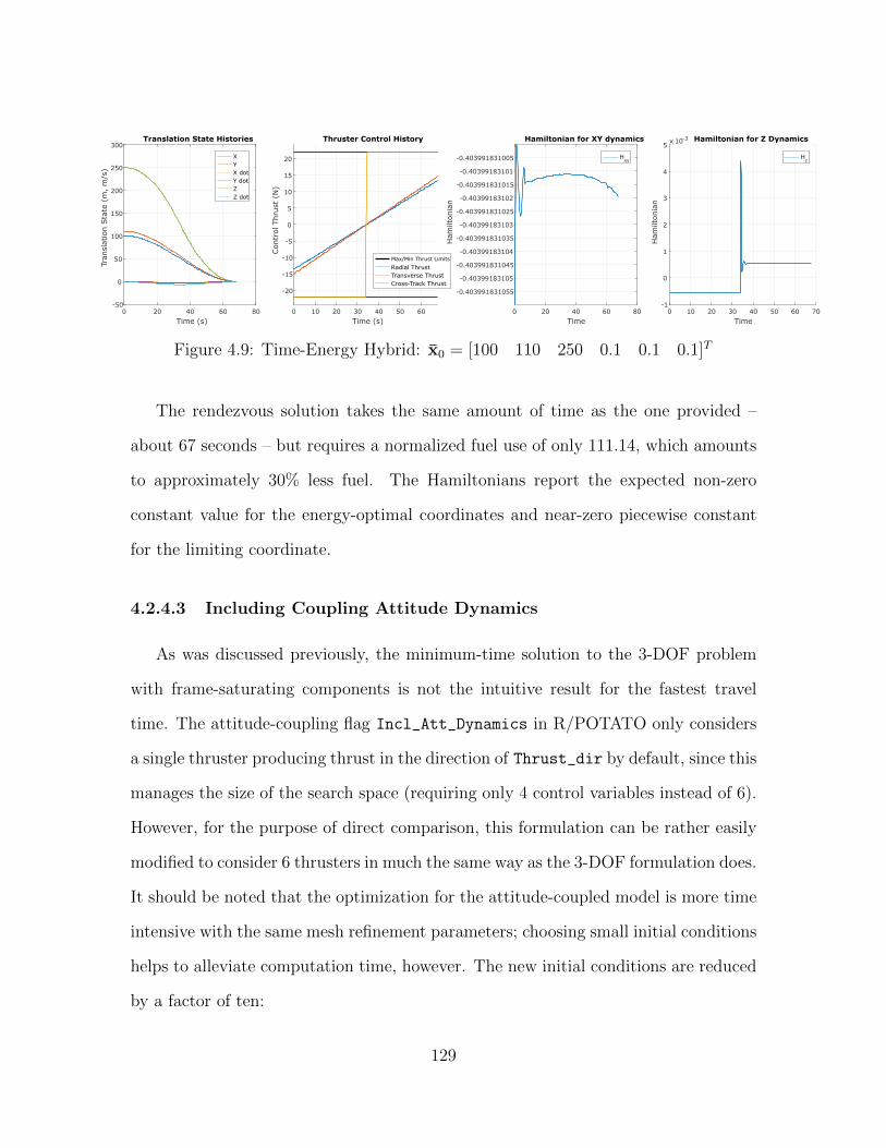
0 20 40 60 80

Time (s)

-50

0

50

100

150

200

250

300

Tran

slat

ion S

tate

(m

, m

/s)

Translation State Histories

XYX dotY dotZZ dot

0 10 20 30 40 50 60

Time (s)

-20

-15

-10

-5

0

5

10

15

20

Con

trol

Thru

st (

N)

Thruster Control History

Max/Min Thrust Limits

Radial ThrustTransverse ThrustCross-Track Thrust

0 20 40 60 80

Time

-0.403991831055

-0.40399183105

-0.403991831045

-0.40399183104

-0.403991831035

-0.40399183103

-0.403991831025

-0.40399183102

-0.403991831015

-0.40399183101

-0.403991831005

Ham

ilton

ian

Hamiltonian for XY dynamics

Hxy

0 10 20 30 40 50 60 70

Time

-1

0

1

2

3

4

5

Ham

ilton

ian

x 10-3 Hamiltonian for Z Dynamics

Hz

Figure 4.9: Time-Energy Hybrid: x0 = [100 110 250 0.1 0.1 0.1]T

The rendezvous solution takes the same amount of time as the one provided –

about 67 seconds – but requires a normalized fuel use of only 111.14, which amounts

to approximately 30% less fuel. The Hamiltonians report the expected non-zero

constant value for the energy-optimal coordinates and near-zero piecewise constant

for the limiting coordinate.

4.2.4.3 Including Coupling Attitude Dynamics

As was discussed previously, the minimum-time solution to the 3-DOF problem

with frame-saturating components is not the intuitive result for the fastest travel

time. The attitude-coupling flag Incl_Att_Dynamics in R/POTATO only considers

a single thruster producing thrust in the direction of Thrust_dir by default, since this

manages the size of the search space (requiring only 4 control variables instead of 6).

However, for the purpose of direct comparison, this formulation can be rather easily

modified to consider 6 thrusters in much the same way as the 3-DOF formulation does.

It should be noted that the optimization for the attitude-coupled model is more time

intensive with the same mesh refinement parameters; choosing small initial conditions

helps to alleviate computation time, however. The new initial conditions are reduced

by a factor of ten:

129

x0 = [10m 11m 25m 0.1m/s 0.1m/s 0.1m/s]T

The 3-DOF min-time problem with these initial conditions, using the scheduling

policy technique, has the following solution:

0 5 10 15 20 25

Time (s)

-5

0

5

10

15

20

25

30

Tran

slat

ion S

tate

(m

, m

/s)

Translation State Histories

XYX dotY dotZZ dot

0 5 10 15 20

Time (s)

-20

-15

-10

-5

0

5

10

15

20

Con

trol

Thru

st (

N)

Thruster Control History

Max/Min Thrust LimitsRadial ThrustTransverse ThrustCross-Track Thrust

0 5 10 15

Time

-8

-6

-4

-2

0

2

4

6

Ham

ilton

ian

x 10-3 Hamiltonian for XY dynamics

Hxy

0 5 10 15 20 25

Time

-3

-2

-1

0

1

2

3

4

5

6

7

Ham

ilton

ian

x 10-3Hamiltonian for Z Dynamics

Hz

Figure 4.10: Scheduling Policy: x0 = [10 11 25 0.1 0.1 0.1]T

The rendezvous occurs in 21.8 seconds, and all thrusters show extremal control,

with the cross-track coordinate limiting the solution time. Coupling attitude dynam-

ics with the same thruster geometry produces the following solution:

0 5 10 15 20

Time (s)

-10

0

10

20

30

Tran

slat

ion

Sta

te(m

,m

/s)

Translation State HistoriesXYZX dotY dotZ dot

0 5 10 15 20

Time (s)

-1

-0.5

0

0.5

1

Quat

ernio

n M

agnitude Quaternion Histories

q1q2q3q4

0 5 10 15 20

Time (s)

-0.2

-0.1

0

0.1

0.2

Rot

atio

n R

ates

(ra

d/s

) Rotation Rate Histories

wxwywz

0 5 10 15 20

Time (s)

-20

-10

0

10

20

Con

trol

Thru

st (

N)

Thruster Control History

Max/Min Thrust LimitsBody X ThrustBody Y ThrustBody Z Thrust

0 5 10 15 20

Time (s)

-1

-0.5

0

0.5

1

Con

trol

Tor

que

(N-m

) Reaction Wheel Torque History

Max/Min TorqueTxTyTz

0 5 10 15 20

Time

-2

-1

0

1

2

Ham

ilton

ian

x 10-3 Hamiltonian

Figure 4.11: 6-Thruster Min-Time w/ Attitude: x0 = [10 11 25 0.1 0.1 0.1]T

with q0 = [0 0 0 1]T and ω0 = [0 0 0]T

This time, rendezvous occurs at approximately 18 seconds. Interestingly, the

130

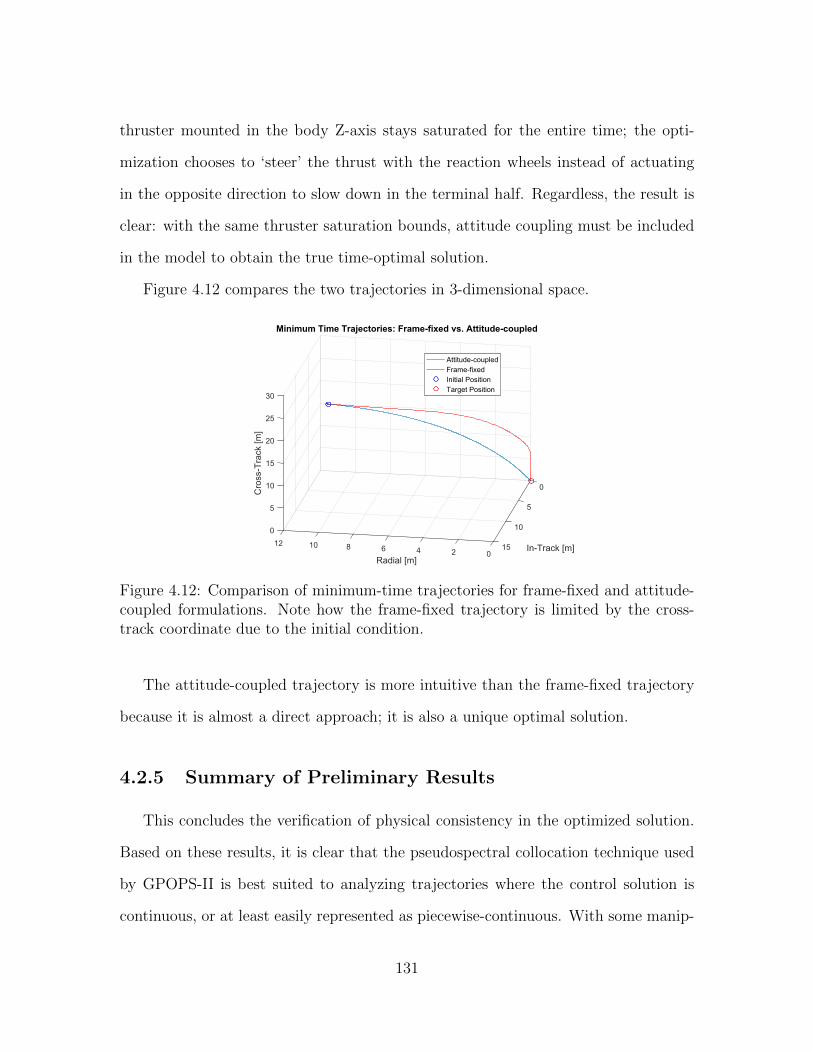
thruster mounted in the body Z-axis stays saturated for the entire time; the opti-

mization chooses to ‘steer’ the thrust with the reaction wheels instead of actuating

in the opposite direction to slow down in the terminal half. Regardless, the result is

clear: with the same thruster saturation bounds, attitude coupling must be included

in the model to obtain the true time-optimal solution.

Figure 4.12 compares the two trajectories in 3-dimensional space.

Figure 4.12: Comparison of minimum-time trajectories for frame-fixed and attitude-coupled formulations. Note how the frame-fixed trajectory is limited by the cross-track coordinate due to the initial condition.

The attitude-coupled trajectory is more intuitive than the frame-fixed trajectory

because it is almost a direct approach; it is also a unique optimal solution.

4.2.5 Summary of Preliminary Results

This concludes the verification of physical consistency in the optimized solution.

Based on these results, it is clear that the pseudospectral collocation technique used

by GPOPS-II is best suited to analyzing trajectories where the control solution is

continuous, or at least easily represented as piecewise-continuous. With some manip-

131

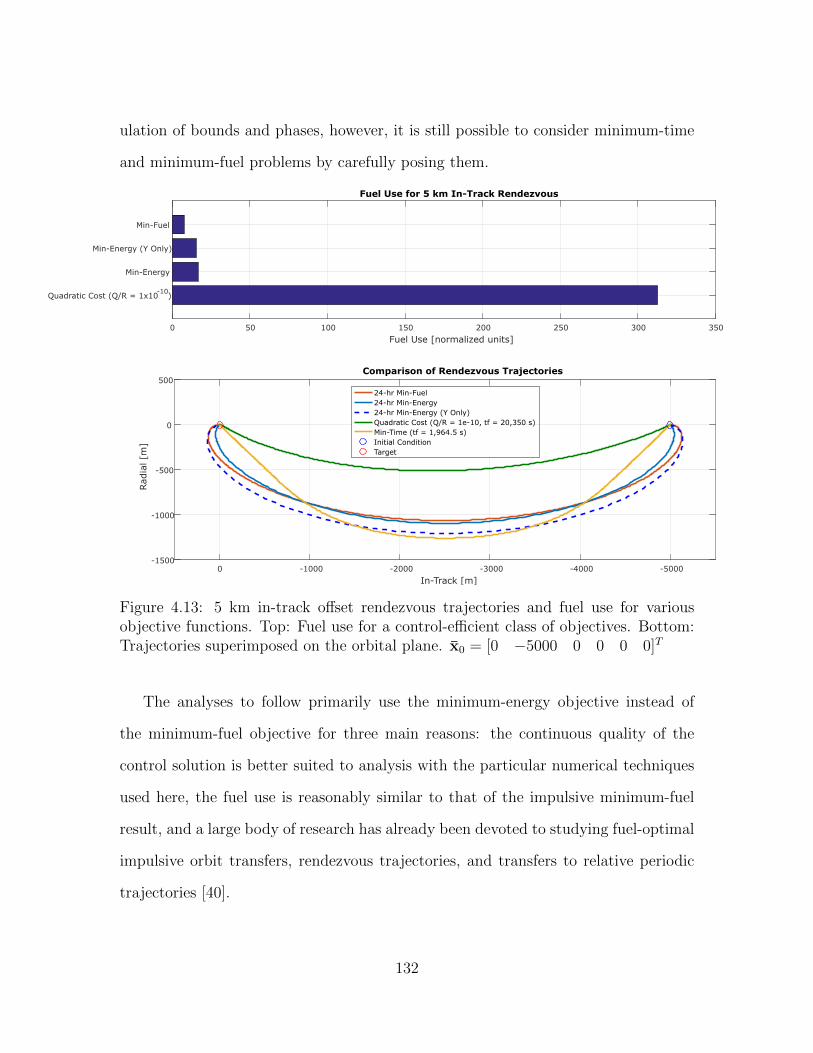
ulation of bounds and phases, however, it is still possible to consider minimum-time

and minimum-fuel problems by carefully posing them.

-1500

-1000

-500

0

500

Rad

ial [m

]

-5000-4000-3000-2000-10000

In-Track [m]

24-hr Min-Fuel24-hr Min-Energy24-hr Min-Energy (Y Only)Quadratic Cost (Q/R = 1e-10, tf = 20,350 s)Min-Time (tf = 1,964.5 s)Initial ConditionTarget

0 50 100 150 200 250 300 350

Fuel Use [normalized units]

Min-Fuel

Min-Energy

Min-Energy (Y Only)

Quadratic Cost (Q/R = 1x10-10

)

Fuel Use for 5 km In-Track Rendezvous

Comparison of Rendezvous Trajectories

Figure 4.13: 5 km in-track offset rendezvous trajectories and fuel use for variousobjective functions. Top: Fuel use for a control-efficient class of objectives. Bottom:Trajectories superimposed on the orbital plane. x0 = [0 −5000 0 0 0 0]T

The analyses to follow primarily use the minimum-energy objective instead of

the minimum-fuel objective for three main reasons: the continuous quality of the

control solution is better suited to analysis with the particular numerical techniques

used here, the fuel use is reasonably similar to that of the impulsive minimum-fuel

result, and a large body of research has already been devoted to studying fuel-optimal

impulsive orbit transfers, rendezvous trajectories, and transfers to relative periodic

trajectories [40].

132

4.3 Demonstration of Path Constraints, Phasing,

and Nonlinear Dynamics

This section reports results from implementations of more interesting problems in

R/POTATO that serve to demonstrate its versatility and build toward the analysis

of efficient, long-duration proximity operations. Implementation of path constraints

is explored in the No-Fly Zone Avoidance problem, where the chaser’s trajectory

must avoid a geometric region of the relative space around the target. Nonlinear dy-

namics and endpoint constraints are put to the test in the Optimal Period Matching

problem, where the chaser must null its secular drift under various scenarios. Fi-

nally, the implementation of the Keplerian relative acceleration model as well as the

true anomaly look-up technique for pre-solving Kepler’s problem is evaluated in the

Highly-Eccentric Rendezvous problem.

4.3.1 No-Fly Zone Avoidance

Path constraints are implemented by specifying the value of the constraint in

Continuous and placing bounds on it in Main. The constraint may be any function of

the states, controls, integrals, or parameters. To demonstrate the usefulness of being

able optimize proximity operations trajectories with path constraints, consider the

minimum-energy rendezvous problem where it is desired to avoid a conical field-of-

view region in the nadir direction of the target.

This problem can be formulated as a normal minimum-energy rendezvous problem

with one path constraint: the chaser’s trajectory must be outside of the no-fly region.

The path value can be encoded as a geometrical function of the state variables as

follows:

133

cFOV = x+

√(y2 + z2) cot2

θFOV + θbuffer2

Where cFOV is the path value which must be strictly positive for locations outside of

a nadir cone that has angular width θFOV . Because this is a numerical tool which

terminates the solution search after the mesh tolerance has been met, an additional

buffer width θbuffer is implemented to guarantee compliance.

The 5-kilometer in-track offset initial condition will be used again in this case

because it is known that the unconstrained minimum-energy solution takes the tra-

jectory directly through the nadir FOV of the target. In addition to the usual flags

for the minimum-energy problem, set Avoid_FOV = 1, FOV = 60, and FOV_buff =

30. The result is shown in Figure 4.14 below.

-2000

-1500

-1000

-500

0

500

Cro

ss-T

rack

[m

]

0

1000

1500

1000

2000

-1000

In-Track [m]

-2000-3000

5000-4000 -500

Radial [m]

-1000-1500-5000 -2000-2500

Target

No-Fly Zone

Min-Energy

Min-Energy with Path Enforcement

0 1 2 3 4 5 6 7 8

Time(s) x 104

-1000

0

1000

2000

3000

4000

5000

6000

7000

8000

9000

Rad

ial D

ispla

cem

ent

from

FO

V C

one

(m)

No-Fly Path Enforcement Comparison

Min-Energy with Path EnforcementMin-EnergyCone BoundaryNo-Fly Violation

3D Relative Trajectory Comparison

Figure 4.14: Avoidance of 60° nadir target field-of-view cone with minimum controlenergy objective. x0 = [0 −5000 0 0 0 0]T

134

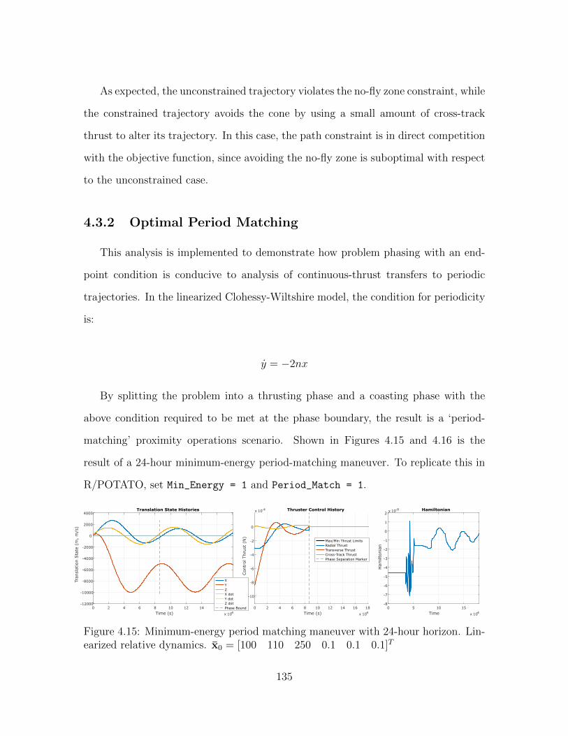
As expected, the unconstrained trajectory violates the no-fly zone constraint, while

the constrained trajectory avoids the cone by using a small amount of cross-track

thrust to alter its trajectory. In this case, the path constraint is in direct competition

with the objective function, since avoiding the no-fly zone is suboptimal with respect

to the unconstrained case.

4.3.2 Optimal Period Matching

This analysis is implemented to demonstrate how problem phasing with an end-

point condition is conducive to analysis of continuous-thrust transfers to periodic

trajectories. In the linearized Clohessy-Wiltshire model, the condition for periodicity

is:

y = −2nx

By splitting the problem into a thrusting phase and a coasting phase with the

above condition required to be met at the phase boundary, the result is a ‘period-

matching’ proximity operations scenario. Shown in Figures 4.15 and 4.16 is the

result of a 24-hour minimum-energy period-matching maneuver. To replicate this in

R/POTATO, set Min_Energy = 1 and Period_Match = 1.

0 2 4 6 8 10 12 14 16 18

Time (s) x 104

-12000

-10000

-8000

-6000

-4000

-2000

0

2000

4000

Tran

slat

ion S

tate

(m

, m

/s)

Translation State Histories

XYZX dotY dotZ dotPhase Bound 0 2 4 6 8 10 12 14 16 18

Time (s) x 104

-10

-8

-6

-4

-2

0

Con

trol

Thru

st (

N)

x 10-4 Thruster Control History

Max/Min Thrust LimitsRadial ThrustTransverse ThrustCross-Track ThrustPhase Separation Marker

0 5 10 15

Time x 104

-8

-7

-6

-5

-4

-3

-2

-1

0

1

2

Ham

ilton

ian

x 10-8 Hamiltonian

Figure 4.15: Minimum-energy period matching maneuver with 24-hour horizon. Lin-earized relative dynamics. x0 = [100 110 250 0.1 0.1 0.1]T

135

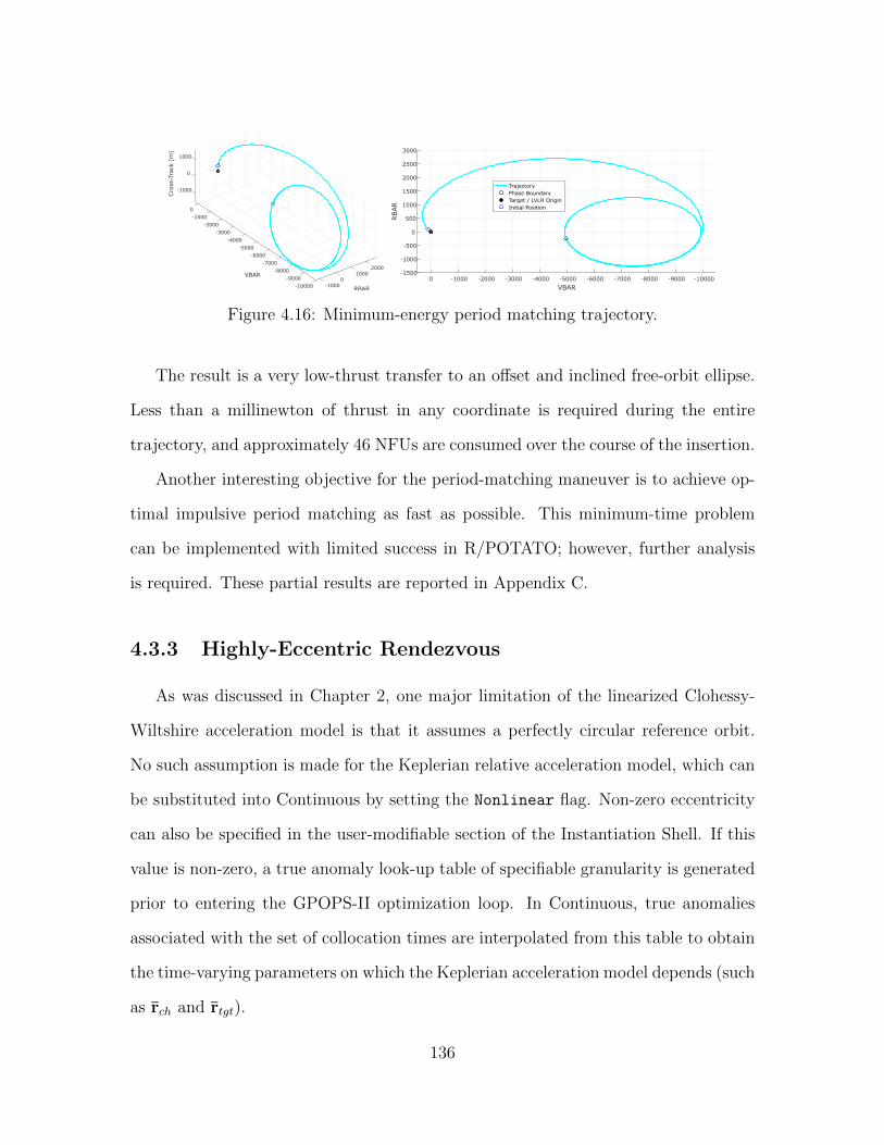
-1500

-1000

-500

0

500

1000

1500

2000

2500

3000

RBAR

-10000-9000-8000-7000-6000-5000-4000-3000-2000-10000

VBAR

TrajectoryPhase BoundaryTarget / LVLH OriginInitial Position

-1000

0

0Cro

ss-T

rack

[m

]

1000

-1000

-2000

-3000

-4000

VBAR

-5000

-6000

-70002000-8000

RBAR

1000-9000 0

-1000-10000

Figure 4.16: Minimum-energy period matching trajectory.

The result is a very low-thrust transfer to an offset and inclined free-orbit ellipse.

Less than a millinewton of thrust in any coordinate is required during the entire

trajectory, and approximately 46 NFUs are consumed over the course of the insertion.

Another interesting objective for the period-matching maneuver is to achieve op-

timal impulsive period matching as fast as possible. This minimum-time problem

can be implemented with limited success in R/POTATO; however, further analysis

is required. These partial results are reported in Appendix C.

4.3.3 Highly-Eccentric Rendezvous

As was discussed in Chapter 2, one major limitation of the linearized Clohessy-

Wiltshire acceleration model is that it assumes a perfectly circular reference orbit.

No such assumption is made for the Keplerian relative acceleration model, which can

be substituted into Continuous by setting the Nonlinear flag. Non-zero eccentricity

can also be specified in the user-modifiable section of the Instantiation Shell. If this

value is non-zero, a true anomaly look-up table of specifiable granularity is generated

prior to entering the GPOPS-II optimization loop. In Continuous, true anomalies

associated with the set of collocation times are interpolated from this table to obtain

the time-varying parameters on which the Keplerian acceleration model depends (such

as rch and rtgt).

136

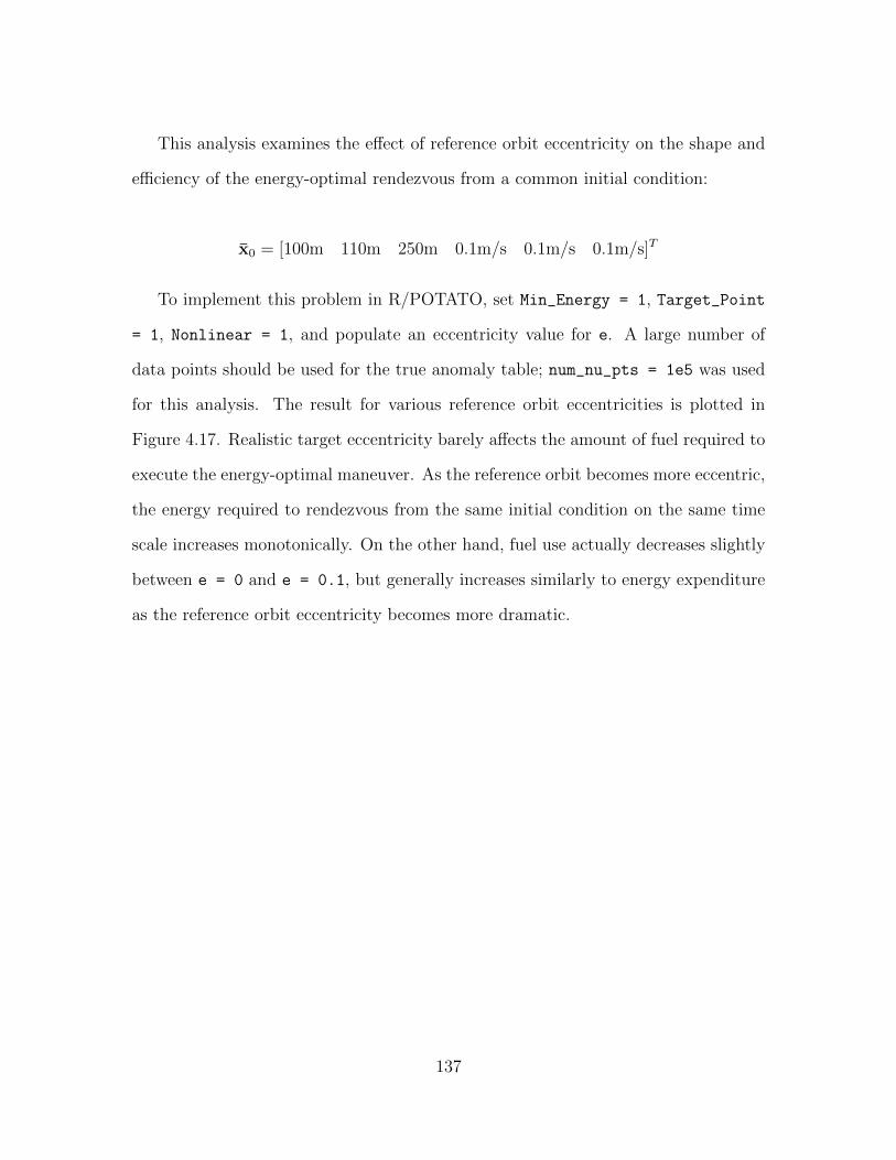
This analysis examines the effect of reference orbit eccentricity on the shape and

efficiency of the energy-optimal rendezvous from a common initial condition:

x0 = [100m 110m 250m 0.1m/s 0.1m/s 0.1m/s]T

To implement this problem in R/POTATO, set Min_Energy = 1, Target_Point

= 1, Nonlinear = 1, and populate an eccentricity value for e. A large number of

data points should be used for the true anomaly table; num_nu_pts = 1e5 was used

for this analysis. The result for various reference orbit eccentricities is plotted in

Figure 4.17. Realistic target eccentricity barely affects the amount of fuel required to

execute the energy-optimal maneuver. As the reference orbit becomes more eccentric,

the energy required to rendezvous from the same initial condition on the same time

scale increases monotonically. On the other hand, fuel use actually decreases slightly

between e = 0 and e = 0.1, but generally increases similarly to energy expenditure

as the reference orbit eccentricity becomes more dramatic.

137

-500

0

500

0

1000

-1000

Min-Energy Trajectories with Different Target Eccentricities

-2000

VBAR

-3000

-4000 1000

RBAR

0-5000-1000

-6000

Initial PositionTargete = 0.000e = 0.005e = 0.100e = 0.300e = 0.500e = 0.700

-1500

-1000

-500

0

500

1000

1500

RBAR

-6000-5000-4000-3000-2000-10000

VBAR

Cro

ss-T

rack

[m

]

0 0.005 0.1 0.3 0.5 0.7

Reference Orbit Eccentricity

0.02

0.04

0.06

0.08

0.1

0.12

0.14

0.16

0.18

0.2

Ener

gy

Exp

enditure

[N

FU2]

100

110

120

130

140

150

160

170

180

Fuel

Use

[N

FU]

Min-Energy Trajectory Efficiency vs. Target Eccentricity

Figure 4.17: Energy-optimal 24-hour rendezvous trajectories from the same initialcondition (left) and fuel and energy expenditure on the energy-optimal trajectory(right) for a range of target eccentricities.

This result (together with the result from the previous analysis on minimum-

fuel trajectories) indicates that while fuel use and energy expenditure are sometimes

comparable as measures of efficiency along the trajectory, an energy-optimal result

can be somewhat less than fuel-optimal. Although the control force is very small, fuel

use grows as a result of integrating over long time periods. This may be a fortuitous

trade for electric propulsion, for which electrical power consumption may overshadow

concerns of fuel capacity.

R/POTATO handles this minimum-energy analysis with nonlinear Keplerian rel-

ative dynamics relatively easily. GPOPS-II and IPOPT are able to determine the

138

24-hour energy-optimal solution in several seconds, even for highly-eccentric targets.

0 2 4 6 8

Time (s) x 104

-6000

-4000

-2000

0

2000

Tran

slat

ion S

tate

(m

,m

/s)

Translation State Histories

XYZX dotY dotZ dot

0 2 4 6 8

Time (s) x 104

-2

-1

0

1

2

Con

trol

Thru

st (

N)

x 10-3 Control History (e = 0.1)Max/Min Thrust LimitsRadial ThrustTransverse ThrustCross-Track Thrust

0 2 4 6 8

Time x 104

-1.5

-1

-0.5

0

Ham

ilton

ian

x 10-6 Hamiltonian

0 2 4 6 8

Time (s) x 104

-6000

-4000

-2000

0

2000

Tran

slat

ion S

tate

(m

, m

/s)

0 2 4 6 8

Time (s) x 104

-2

-1

0

1

2

Con

trol

Thru

st (

N)

x 10-3 Control History (e = 0.3)

0 2 4 6 8

Time x 104

-4

-2

0

2

4

6

Ham

ilton

ian

x 10-6

0 2 4 6 8

Time (s) x 104

-6000

-4000

-2000

0

2000

Tran

slat

ion S

tate

(m

, m

/s)

0 2 4 6 8

Time (s) x 104

-2

-1

0

1

2

Con

trol

Thru

st (

N)

x 10-3 Control History (e = 0.5)

0 2 4 6 8

Time x 104

-1

0

1

2

3

Ham

ilton

ian

x 10-5

0 2 4 6 8

Time (s) x 104

-8000

-6000

-4000

-2000

0

2000

Tran

slat

ion S

tate

(m

, m

/s)

0 2 4 6 8

Time (s) #104

-2

-1

0

1

2

Con

trol

Thru

st (

N)

x 10-3 Control History (e = 0.7)

0 2 4 6 8

Time x 104

-1

0

1

2

3

Ham

ilton

ian

x 10-4

Figure 4.18: Evolution of the energy-optimal control as reference orbit eccentricity isincreased. x0 = [100 110 250 0.1 0.1 0.1]T

Note how the energy-optimal solution changes as reference orbit eccentricity in-

creases: the solution appears to be a sinusoid section in the circular case, but gradually

becomes distorted in a way that mirrors eccentric state trajectories (as can be seen

in Figure 2.15 or B.1, for example). Although the dynamics are no longer LTI, the

139

control still enters linearly into the acceleration model, and thus the optimal control is

still a linear function of the costate solution (which can be thought of as a dual set of

dynamics to the state). In other words, the optimal control policy obtained as the re-

sult of the analysis in subsection 3.1.1.1 is exactly the same in this case, although the

costate solution is obtained as the result of a much more difficult-to-analyze two-point

boundary value problem.

4.3.4 Summary of Intermediate Results

The analyses in this section built upon the foundation of the first section by imple-

menting path constraints, multiple phases, endpoint dynamics, and nonlinear kine-

matics. Each scenario demonstrated a piece of this advanced level of implementation

in a stepping-stone approach to the main scenario of interest in this thesis, which is

long-duration proximity operations. Based on the results from these first two sections,

the best outcome is expected from posing this as a multiple-phase minimum-energy

problem.

4.4 Long-Duration Proximity Operations

In this section, results from the implementation of minimum-energy trajectories

including circumnavigating free-orbit sections are presented. In the first subsection,

methods for specifying the size and orientation of the free-orbit trajectory based on

the techniques explored in Chapter 2 are presented as endpoint constraints for both

the linearized Clohessy-Wiltshire dynamics and the nonlinear Keplerian dynamics. In

the second subsection, a final ‘cost of linearization’ analysis is performed where fuel

use is characterized for a chaser attempting to enforce the geometry of a Clohessy-

Wiltshire ellipse in a Keplerian relative acceleration model.

140

4.4.1 Free-Orbit Trajectory Design

4.4.1.1 Clohessy-Wiltshire Relative Dynamics

Chapter 2 describes the various ways that free-orbit trajectories can be sized in

oriented in the LVLH frame. For close-range proximity operations, linearization error

may be tolerable and the HCW model a desirable tool for on-line computations. For

this reason, it is helpful to be able to analyze and parameterize periodic trajectories

in this model. Under the linearizing assumptions of the Clohessy-Wiltshire model, all

periodic trajectories project a 2-by-1 ellipse onto the orbital plane and are symmetric

about the in-track axis. The center of the ellipse need not be coincident with the

LVLH origin, and in fact may be offset anywhere along the in-track axis. The ellipse

can also be inclined in the cross-track coordinate about this axis.

The user may specify Target_Ellipse to analyze a trajectory with an insertion

phase and a free-orbit phase. The size of the free-orbit ellipse can be specified as

alpha, which is the desired semimajor axis of the relative trajectory. The cross-track

inclination of the trajectory can be specified as zeta. The nodal azimuth of the local

ascending node can be specified as gamma. The location of the ellipse’s center can be

specified with Vbar_Offset. These design parameters can either be encoded in the

Endpoint function as constraints on the LVLH state variables at the terminus of the

transfer phase, or as path constraints which are enforced for the duration of the free-

orbit phase; this can be chosen by setting the flag coast. If it is set to 1, endpoint

constraints are activated while prohibiting thrust in the second phase, otherwise the

path constraint approach is used.

The following results can be obtained by setting Target_Ellipse = 1, alpha =

1000, zeta = 0, gamma = 0, VbarOffset = 0, and coast = 1. Three stationary

initial conditions are analyzed: a 5-kilometer offset purely in the in-track, radial, and

141

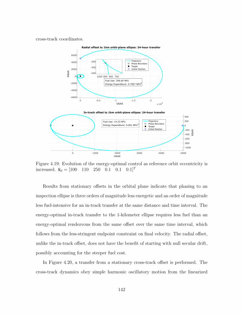
cross-track coordinates.

-6000

-4000

-2000

0

2000

4000

6000

RBAR

-2-1.5-1-0.50

VBAR x 104

Radial offset to 1km orbit-plane ellipse: 24-hour transfer

TrajectoryPhase BoundaryTargetInitial Position

-400

-300

-200

7008009001000

Fuel Use: 356.60 NFU

Energy Expenditure: 0.7857 NFU2

-1000

-800

-600

-400

-200

0

200

400

RBAR

-5000-4000-3000-2000-10000

VBAR

In-track offset to 1km orbit-plane ellipse: 24-hour transfer

TrajectoryPhase BoundaryTargetInitial Position

Fuel Use: 14.23 NFU

Energy Expenditure: 0.001 NFU2

Figure 4.19: Evolution of the energy-optimal control as reference orbit eccentricity isincreased. x0 = [100 110 250 0.1 0.1 0.1]T

Results from stationary offsets in the orbital plane indicate that phasing to an

inspection ellipse is three orders of magnitude less energetic and an order of magnitude

less fuel-intensive for an in-track transfer at the same distance and time interval. The

energy-optimal in-track transfer to the 1-kilometer ellipse requires less fuel than an

energy-optimal rendezvous from the same offset over the same time interval, which

follows from the less-stringent endpoint constraint on final velocity. The radial offset,

unlike the in-track offset, does not have the benefit of starting with null secular drift,

possibly accounting for the steeper fuel cost.

In Figure 4.20, a transfer from a stationary cross-track offset is performed. The

cross-track dynamics obey simple harmonic oscillatory motion from the linearized

142

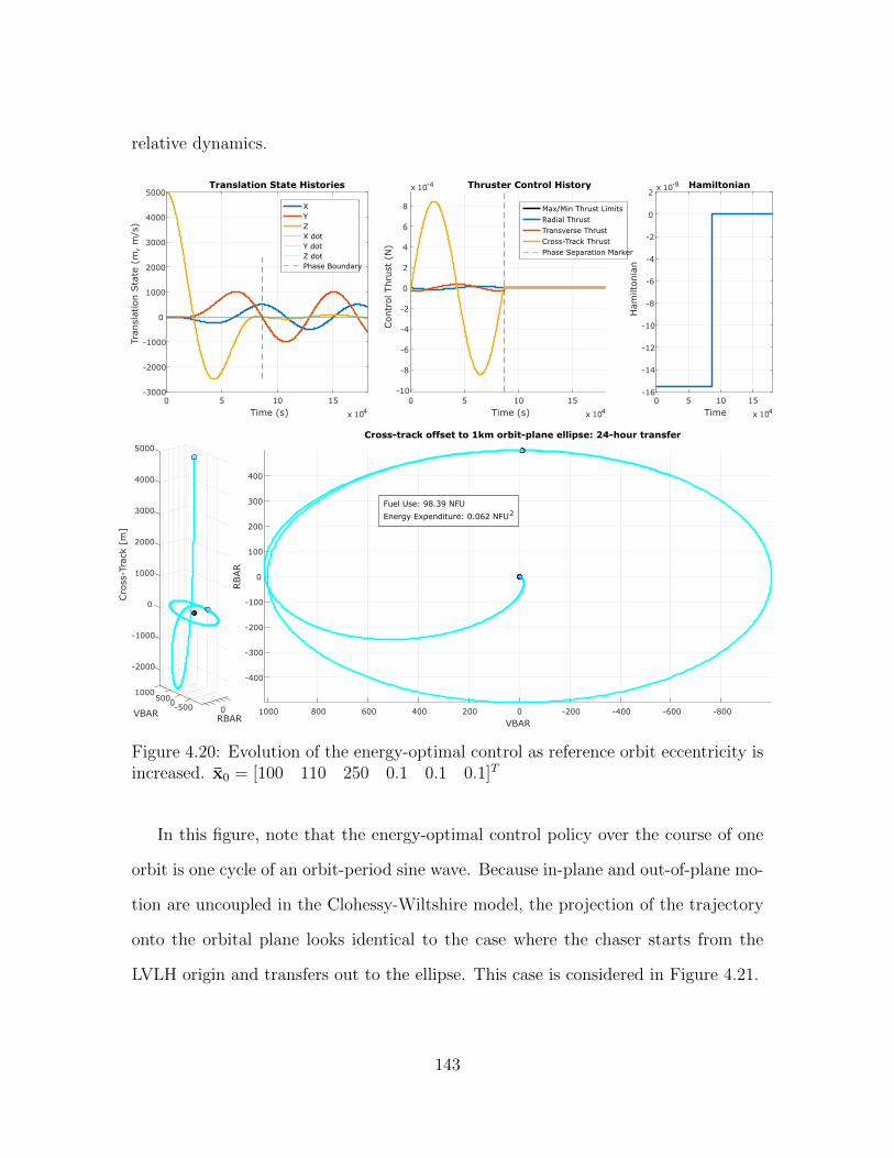
relative dynamics.

-2000

1000

-1000

500

0

VBAR

1000

0

RBAR

2000

Cro

ss-T

rack

[m

]

-500 0

3000

4000

5000

-400

-300

-200

-100

0

100

200

300

400

RBAR

-800-600-400-20002004006008001000

VBAR

Fuel Use: 98.39 NFU

Energy Expenditure: 0.062 NFU2

0 5 10 15

Time (s) x 104

-3000

-2000

-1000

0

1000

2000

3000

4000

5000

Tran

slat

ion S

tate

(m

, m

/s)

Translation State Histories

XYZX dotY dotZ dotPhase Boundary

0 5 10 15

Time (s) x 104

-10

-8

-6

-4

-2

0

2

4

6

8

Con

trol

Thru

st (

N)

x 10-4 Thruster Control History

Max/Min Thrust LimitsRadial ThrustTransverse ThrustCross-Track ThrustPhase Separation Marker

0 5 10 15

Time x 104

-16

-14

-12

-10

-8

-6

-4

-2

0

2

Ham

ilton

ian

x 10-8 Hamiltonian

Cross-track offset to 1km orbit-plane ellipse: 24-hour transfer

Figure 4.20: Evolution of the energy-optimal control as reference orbit eccentricity isincreased. x0 = [100 110 250 0.1 0.1 0.1]T

In this figure, note that the energy-optimal control policy over the course of one

orbit is one cycle of an orbit-period sine wave. Because in-plane and out-of-plane mo-

tion are uncoupled in the Clohessy-Wiltshire model, the projection of the trajectory

onto the orbital plane looks identical to the case where the chaser starts from the

LVLH origin and transfers out to the ellipse. This case is considered in Figure 4.21.

143

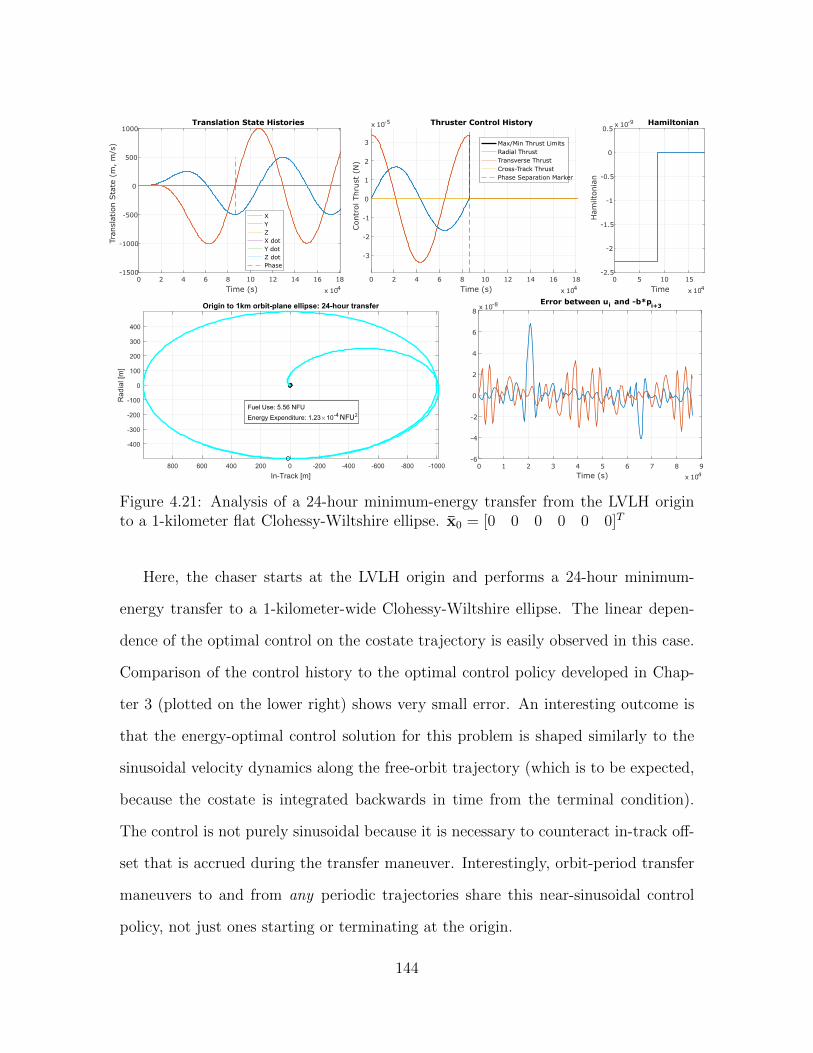
0 1 2 3 4 5 6 7 8 9Time (s) x 104

-6

-4

-2

0

2

4

6

8x 10-8 Error between ui and -b*p

i+3

0 2 4 6 8 10 12 14 16 18

Time (s) x 104

-1500

-1000

-500

0

500

1000

Tran

slat

ion S

tate

(m

, m

/s)

Translation State Histories

XYZX dotY dotZ dotPhase

0 2 4 6 8 10 12 14 16 18

Time (s) x 104

-3

-2

-1

0

1

2

3

Con

trol

Thru

st (

N)

x 10-5 Thruster Control History

Max/Min Thrust LimitsRadial ThrustTransverse ThrustCross-Track ThrustPhase Separation Marker

0 5 10 15

Time x 104

-2.5

-2

-1.5

-1

-0.5

0

0.5

Ham

ilton

ian

x 10-9 Hamiltonian

NFU2

Figure 4.21: Analysis of a 24-hour minimum-energy transfer from the LVLH originto a 1-kilometer flat Clohessy-Wiltshire ellipse. x0 = [0 0 0 0 0 0]T

Here, the chaser starts at the LVLH origin and performs a 24-hour minimum-

energy transfer to a 1-kilometer-wide Clohessy-Wiltshire ellipse. The linear depen-

dence of the optimal control on the costate trajectory is easily observed in this case.

Comparison of the control history to the optimal control policy developed in Chap-

ter 3 (plotted on the lower right) shows very small error. An interesting outcome is

that the energy-optimal control solution for this problem is shaped similarly to the

sinusoidal velocity dynamics along the free-orbit trajectory (which is to be expected,

because the costate is integrated backwards in time from the terminal condition).

The control is not purely sinusoidal because it is necessary to counteract in-track off-

set that is accrued during the transfer maneuver. Interestingly, orbit-period transfer

maneuvers to and from any periodic trajectories share this near-sinusoidal control

policy, not just ones starting or terminating at the origin.

144

0 5 10 15

Time (s) x 104

-15000

-10000

-5000

0

5000Tr

ansl

atio

n S

tate

(m

, m

/s) Translation State Histories

XYZX dotY dotZ dotPhase Boundary

0 5 10 15

Time (s) x 104

-3

-2

-1

0

1

2

3

Con

trol

Thru

st (

N)

x 10-4 Thruster Control HistoryMax/Min Thrust LimitsRadial ThrustTransverse ThrustCross-Track ThrustPhase Marker

0 5 10 15

Time x 104

-1.795

-1.794

-1.793

-1.792

-1.791

Ham

ilton

ian

x 10-7 Hamiltonian

-4000

-3000

-2000

-1000

0

1000

2000

3000

4000

5000

Rad

ial [m

]

-10000-8000-6000-4000-200002000400060008000

In-Track [m]

Fuel Use: 50.065 NFU

Energy Expenditure: 0.0100 NFU2

Figure 4.22: 24-hour transfer from a 10-kilometer ellipse to a 1-kilometer ellipse.Note the similarity in the control history to the origin-to-1-kilometer ellipse transfer.x0 = [100 110 250 0.1 0.1 0.1]T

This concept is demonstrated in Figure 4.22, where the chaser starts from the

maximum radial offset in a 10-kilometer ellipse, and must transfer to a 1-kilometer

ellipse over the course of one orbit. The energy-optimal result involves thrust in the

hundreds of micronewtons following a similar control policy, which is approximately

sinusoidal and proportional to the difference in the velocity dynamics between the

same angular locations on the initial and final trajectories. If in-track offset in the

resulting trajectory is tolerable, it may be desirable to use simple sinusoids in the

control policy for the sake of simplicity and the minuscular and slowly-changing thrust

required to execute it, making it ideal for formation fliers using electric propulsion.

Using MATLAB and Simulink, it can be shown that open-loop simple-sinusoid control

actuated at the appropriate times consistently results in a periodic transfer maneuver.

145

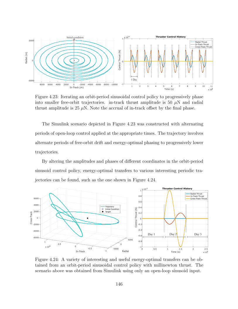
-5000

0

5000

Rad

ial (m

)

-10000-8000-6000-4000-200002000400060008000

In-Track (m)

Initial condition

x

1 2 3 4 5 6 7 8 9 10 11

Time (s) x 105

-1

0

1

Con

trol

Thru

st (

N)

x 10-4 Thruster Control History

Radial ThrustIn-Track ThrustCross-Track Thrust

1 Day

Figure 4.23: Iterating an orbit-period sinusoidal control policy to progressively phaseinto smaller free-orbit trajectories. in-track thrust amplitude is 50 µN and radialthrust amplitude is 25 µN. Note the accrual of in-track offset by the final phase.

The Simulink scenario depicted in Figure 4.23 was constructed with alternating

periods of open-loop control applied at the appropriate times. The trajectory involves

alternate periods of free-orbit drift and energy-optimal phasing to progressively lower

trajectories.

By altering the amplitudes and phases of different coordinates in the orbit-period

sinusoid control policy, energy-optimal transfers to various interesting periodic tra-

jectories can be found, such as the one shown in Figure 4.24.

-60005000

-4000

-2000

0

Cro

ss-T

rack

2000

1

4000

6000

Radial

0.5 0x 104

In-Track

0-0.5 -5000

-1

TrajectoryInitial ConditionTarget

0 0.5 1 1.5 2 2.5

Time (s) x 105

-1

-0.8

-0.6

-0.4

-0.2

0

0.2

0.4

0.6

0.8

1

Con

trol

Thru

st (

N)

x 10-3 Thruster Control History

Radial ThrustIn-Track ThrustCross-Track Thrust

Day 1 Day 2 Day 3

Figure 4.24: A variety of interesting and useful energy-optimal transfers can be ob-tained from an orbit-period sinusoidal control policy with millinewton thrust. Thescenario above was obtained from Simulink using only an open-loop sinusoid input.

146

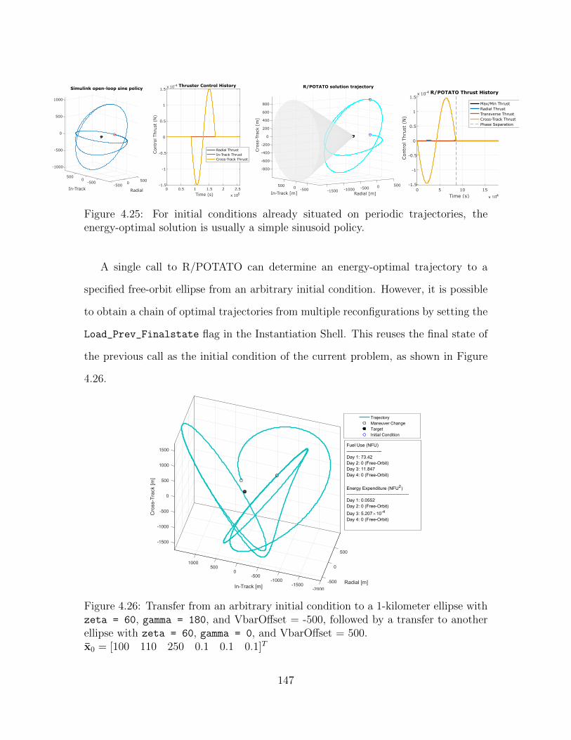
-1000

-500

0

500

1000

500

Simulink open-loop sine policy

In-Track

0 500

Radial

-500 0-500

0 0.5 1 1.5 2 2.5

Time (s) x 105

-1.5

-1

-0.5

0

0.5

1

1.5

Con

trol

Thru

st (

N)

x 10-4 Thruster Control History

Radial ThrustIn-Track ThrustCross-Track Thrust

0 5 10 15

Time (s) x 104

-1.5

-1

-0.5

0

0.5

1

1.5

Con

trol

Thru

st (

N)

x 10-4 R/POTATO Thrust History

Max/Min ThrustRadial ThrustTransverse ThrustCross-Track ThrustPhase Separation

-800

-600

-400

-200

0

200

400

600

800

Cro

ss-T

rack

[m

]

R/POTATO solution trajectory

500500 00

In-Track [m]-500

Radial [m]-1000-500 -1500

Figure 4.25: For initial conditions already situated on periodic trajectories, theenergy-optimal solution is usually a simple sinusoid policy.

A single call to R/POTATO can determine an energy-optimal trajectory to a

specified free-orbit ellipse from an arbitrary initial condition. However, it is possible

to obtain a chain of optimal trajectories from multiple reconfigurations by setting the

Load_Prev_Finalstate flag in the Instantiation Shell. This reuses the final state of

the previous call as the initial condition of the current problem, as shown in Figure

4.26.

Figure 4.26: Transfer from an arbitrary initial condition to a 1-kilometer ellipse withzeta = 60, gamma = 180, and VbarOffset = -500, followed by a transfer to anotherellipse with zeta = 60, gamma = 0, and VbarOffset = 500.x0 = [100 110 250 0.1 0.1 0.1]T

147

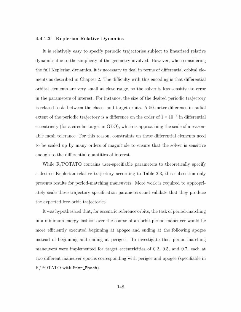
4.4.1.2 Keplerian Relative Dynamics

It is relatively easy to specify periodic trajectories subject to linearized relative

dynamics due to the simplicity of the geometry involved. However, when considering

the full Keplerian dynamics, it is necessary to deal in terms of differential orbital ele-

ments as described in Chapter 2. The difficulty with this encoding is that differential

orbital elements are very small at close range, so the solver is less sensitive to error

in the parameters of interest. For instance, the size of the desired periodic trajectory

is related to δe between the chaser and target orbits. A 50-meter difference in radial

extent of the periodic trajectory is a difference on the order of 1× 10−6 in differential

eccentricity (for a circular target in GEO), which is approaching the scale of a reason-

able mesh tolerance. For this reason, constraints on these differential elements need

to be scaled up by many orders of magnitude to ensure that the solver is sensitive

enough to the differential quantities of interest.

While R/POTATO contains user-specifiable parameters to theoretically specify

a desired Keplerian relative trajectory according to Table 2.3, this subsection only

presents results for period-matching maneuvers. More work is required to appropri-

ately scale these trajectory specification parameters and validate that they produce

the expected free-orbit trajectories.

It was hypothesized that, for eccentric reference orbits, the task of period-matching

in a minimum-energy fashion over the course of an orbit-period maneuver would be

more efficiently executed beginning at apogee and ending at the following apogee

instead of beginning and ending at perigee. To investigate this, period-matching

maneuvers were implemented for target eccentricities of 0.2, 0.5, and 0.7, each at

two different maneuver epochs corresponding with perigee and apogee (specifiable in

R/POTATO with Mnvr_Epoch).

148

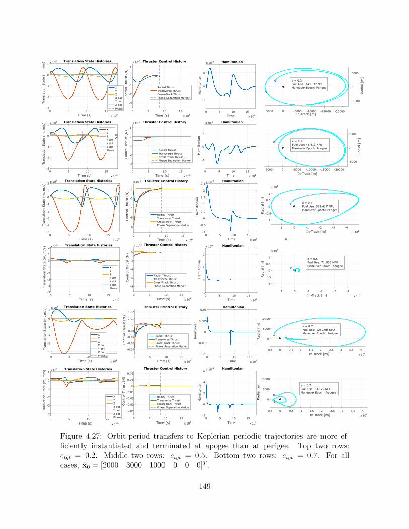
0 5 10 15

Time (s) x 104

-5

-4

-3

-2

-1

0

1

2

Tran

slat

ion S

tate

(m

, m

/s)

x 104 Translation State Histories

0 5 10 15

Time (s) x 104

-8

-6

-4

-2

0

Con

trol

Thru

st (

N)

x 10-3 Thruster Control History

Radial ThrustTransverse ThrustCross-Track ThrustPhase Separation Marker

0 5 10 15

Time x 104

-1

-0.5

0

0.5

1

1.5

2

2.5

Ham

ilton

ian

x 10-4 Hamiltonian

-1

-0.5

0

0.5

1

Rad

ial [m

]

x 104

-4-3-2-101

In-Track [m] x 104

e = 0.5Fuel Use: 382.617 NFUManeuver Epoch: Perigee

0 5 10 15

Time (s) x 104

-5

-4

-3

-2

-1

0

1

2

Tran

slat

ion S

tate

(m

, m

/s) x 104 Translation State Histories

XYZX dotY dotZ dotPhase

0 5 10 15

Time (s) x 104

-8

-6

-4

-2

0

Con

trol

Thru

st (

N)

x 10-3 Thruster Control History

Radial ThrustTransverse ThrustCross-Track ThrustPhase Separation Marker

0 5 10 15

Time x 104

-1

0

1

2

Ham

ilton

ian

x 10-4 Hamiltonian

-1

-0.5

0

0.5

1

Rad

ial [m

]

x 104

-4-3-2-101

In-Track [m] x 104

e = 0.5Fuel Use: 71.836 NFUManeuver Epoch: Apogee

0 5 10 15

Time (s) x 104

-4

-3

-2

-1

0

1

Tran

slat

ion S

tate

(m

, m

/s) x 104 Translation State Histories

XYZX dotY dotZ dotPhase 0 5 10 15

Time (s) x 104

-0.04

-0.03

-0.02

-0.01

0

0.01

0.02

Con

trol

Thru

st (

N)

Thruster Control History

Radial ThrustTransverse ThrustCross-Track ThrustPhase Separation Marker

0 5 10 15

Time x 104

-0.01

-0.005

0

0.005

0.01

Ham

ilton

ian

Hamiltonian

0

5000

10000

Rad

ial [m

]

-4-3.5-3-2.5-2-1.5-1-0.500.5

In-Track [m] x 104

e = 0.7Fuel Use: 1280.96 NFUManeuver Epoch: Perigee

0 5 10 15

Time (s) x 104

-4

-3

-2

-1

0

1

Tran

slat

ion S

tate

(m

, m

/s) x 104 Translation State Histories

XYZX dotY dotZ dotPhase 0 5 10 15

Time (s) x 104

-0.04

-0.03

-0.02

-0.01

0

0.01

0.02

Con

trol

Thru

st (

N)

Thruster Control History

Radial ThrustTransverse ThrustCross-Track ThrustPhase Separation Marker

0 5 10 15

Time (s) x 104

-3

-2

-1

0

1

Tran

slat

ion S

tate

(m

, m

/s) x 104 Translation State Histories

XYZX dotY dotZ dotPhase

0 5 10 15

Time (s) x 104

-3

-2

-1

0

1

Con

trol

Thru

st (

N)

x 10-3 Thruster Control History

Radial ThrustTransverse ThrustCross-Track ThrustPhase Separation Marker

0 5 10 15

Time x 104

-5

0

5

Ham

ilton

ian

x 10-6 Hamiltonian

-15000-10000

Rad

ial [m

]

5000

0

05000In-Track [m]

-5000

-5000

-20000

e = 0.2Fuel Use: 143.837 NFUManeuver Epoch: Perigee

0 5 10 15

Time (s) x 104

-3

-2

-1

0

1

Tran

slat

ion S

tate

(m

, m

/s) x 104 Translation State Histories

XYZX dotY dotZ dotPhase

0 5 10 15

Time (s) x 104

-3

-2

-1

0

1Con

trol

Thru

st (

N)

x 10-3 Thruster Control History

Radial ThrustTransverse ThrustCross-Track ThrustPhase Separation Marker

0 5 10 15

Time x 104

-5

0

5

Ham

ilton

ian

#10-6 Hamiltonian

-5000

0

5000

Rad

ial [m

]

-20000-15000-10000-500005000

In-Track [m]

e = 0.2Fuel Use: 45.413 NFUManeuver Epoch: Apogee

0 5 10 15

Time x 104

-2

0

2

4

6

Ham

ilton

ian

x 10-4 Hamiltonian

0

5000

10000

Rad

ial [m

]

-4-3.5-3-2.5-2-1.5-1-0.500.5

In-Track [m] x 104

e = 0.7Fuel Use: 63.129 NFUManeuver Epoch: Apogee

Figure 4.27: Orbit-period transfers to Keplerian periodic trajectories are more ef-ficiently instantiated and terminated at apogee than at perigee. Top two rows:etgt = 0.2. Middle two rows: etgt = 0.5. Bottom two rows: etgt = 0.7. For allcases, x0 = [2000 3000 1000 0 0 0]T .

149

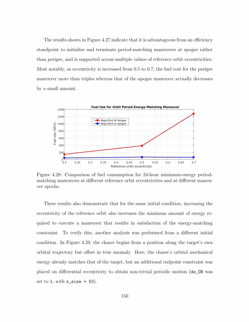
The results shown in Figure 4.27 indicate that it is advantageous from an efficiency

standpoint to initialize and terminate period-matching maneuvers at apogee rather

than perigee, and is supported across multiple values of reference orbit eccentricities.

Most notably, as eccentricity is increased from 0.5 to 0.7, the fuel cost for the perigee

maneuver more than triples whereas that of the apogee maneuver actually decreases

by a small amount.

0.2 0.25 0.3 0.35 0.4 0.45 0.5 0.55 0.6 0.65 0.7

Reference orbit eccentricity

0

200

400

600

800

1000

1200

1400

Fuel

Use

(N

FU)

Fuel Use for Orbit Period Energy-Matching Maneuver

Begin/End at PerigeeBegin/End at Apogee

Figure 4.28: Comparison of fuel consumption for 24-hour minimum-energy period-matching maneuvers at different reference orbit eccentricities and at different maneu-ver epochs.

These results also demonstrate that for the same initial condition, increasing the

eccentricity of the reference orbit also increases the minimum amount of energy re-

quired to execute a maneuver that results in satisfaction of the energy-matching

constraint. To verify this, another analysis was performed from a different initial

condition. In Figure 4.29, the chaser begins from a position along the target’s own

orbital trajectory but offset in true anomaly. Here, the chaser’s orbital mechanical

energy already matches that of the target, but an additional endpoint constraint was

placed on differential eccentricity to obtain non-trivial periodic motion (de_ON was

set to 1, with x_size = 50).

150

0 5 10 15

Time (s) x 104

-2

-1.5

-1

-0.5

0

0.5

1

1.5

Tran

slat

ion S

tate

(m

, m

/s) x 104 Translation State Histories

XYZX dotY dotZ dotPhase 0 5 10 15

Time (s) x 104

-6

-4

-2

0

2

Con

trol

Thru

st (

N)

x 10-3 Thruster Control History

Radial ThrustTransverse ThrustCross-Track ThrustPhase Separation Marker

0 5 10 15

Time x 104

-1.5

-1

-0.5

0

0.5

1

1.5

2

Ham

ilton

ian

x 10-3 Hamiltonian

-5000

0

5000

Rad

ial [m

]

-1.5-1-0.500.51

In-Track [m] x 104

e = 0.7Fuel Use: 198.6571 NFU

0 5 10 15

Time (s) x 104

-6000

-4000

-2000

0

2000

4000

Tran

slat

ion S

tate

(m

, m

/s) Translation State Histories

0 5 10 15

Time (s) x 104

-1

-0.5

0

0.5

1

1.5

Con

trol

Thru

st (

N)

x 10-4 Thruster Control History

Radial ThrustTransverse ThrustCross-Track ThrustPhase Separation Marker

0 5 10 15

Time x 104

-1.5

-1

-0.5

0

0.5

1

Ham

ilton

ian

x 10-7 Hamiltonian

-2000

-1000

0

1000

Rad

ial [m

]

-5000-4000-3000-2000-10000100020003000

In-Track [m]

e = 0.1Fuel Use: 15.8248 NFU

Figure 4.29: Transfers to Keplerian periodic trajectories. Top: etgt = 0.1. Bottom:etgt = 0.7. For both cases, x0 = [−0.0351 −5000 0 0 0 0]T

This analysis from a different initial condition corroborates the previous one, show-

ing greater fuel use to period-match in the case of higher eccentricity.

4.4.2 Cost of Linearization Revisited

The final analysis performed with R/POTATO re-examines the ‘cost of lineariza-

tion’ investigation from Chapter 2, but from the standpoint of fuel use. In this

scenario, the chaser’s objective function is an LQR-like function of position error and

control energy expenditure, with relative weighting that is control-averse.

J =1

2

∫ tf

t0

1× 10−6 ·(x2 + y2 + z2

)+ (u2x + u2y + u2z) dt

Position errors x, y, and z are measured with respect to a pre-defined Clohessy-

Wiltshire free-orbit ellipse. Because the scenario is subject to nonlinear Keplerian

relative dynamics, the chaser must expend formation-keeping control effort to main-

tain the linearized elliptical trajectory. Although the objective is control-averse, an

151

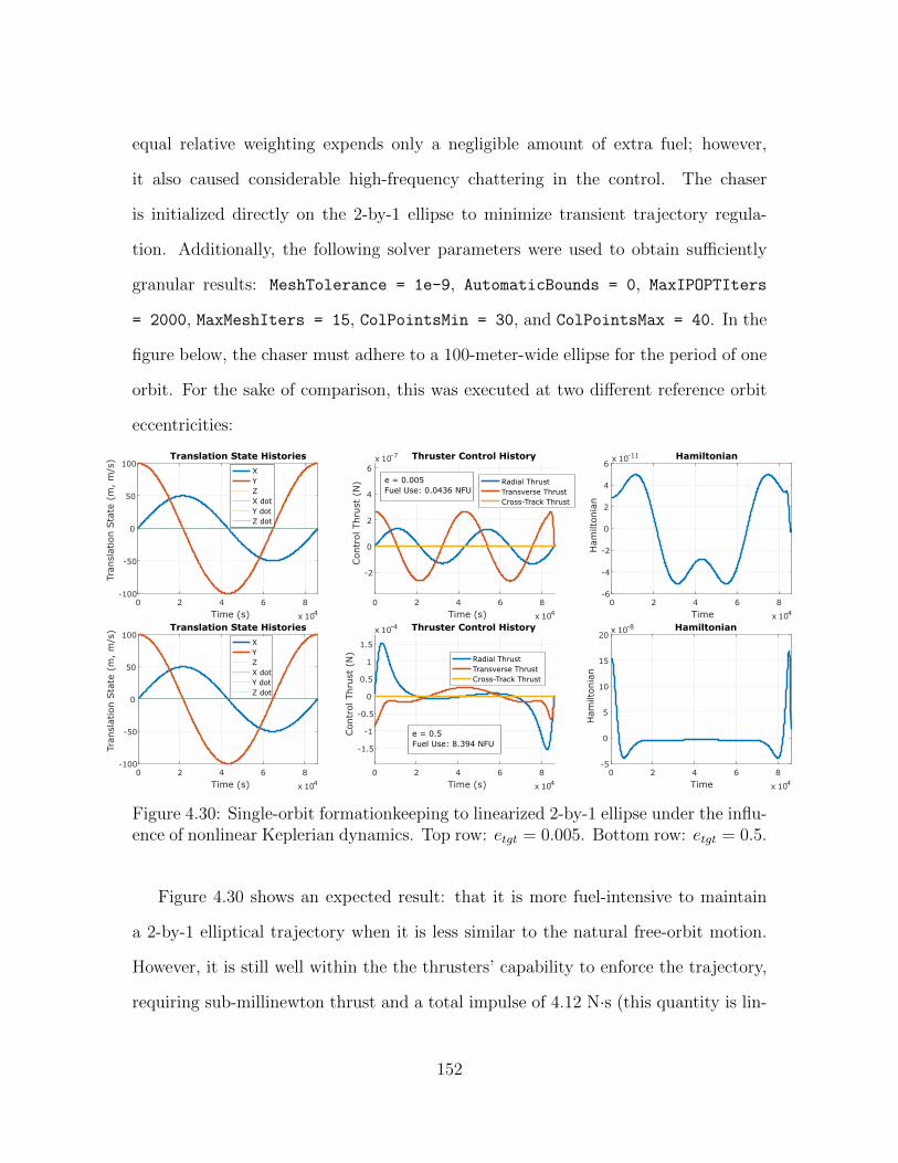
equal relative weighting expends only a negligible amount of extra fuel; however,

it also caused considerable high-frequency chattering in the control. The chaser

is initialized directly on the 2-by-1 ellipse to minimize transient trajectory regula-

tion. Additionally, the following solver parameters were used to obtain sufficiently

granular results: MeshTolerance = 1e-9, AutomaticBounds = 0, MaxIPOPTIters

= 2000, MaxMeshIters = 15, ColPointsMin = 30, and ColPointsMax = 40. In the

figure below, the chaser must adhere to a 100-meter-wide ellipse for the period of one

orbit. For the sake of comparison, this was executed at two different reference orbit

eccentricities:

0 2 4 6 8

Time (s) x 104

-100

-50

0

50

100

Tran

slat

ion S

tate

(m

, m

/s) Translation State Histories

XYZX dotY dotZ dot

0 2 4 6 8

Time (s) x 104

-2

0

2

4

6

Con

trol

Thru

st (

N)

x 10-7 Thruster Control History

Radial ThrustTransverse ThrustCross-Track Thrust

0 2 4 6 8

Time x 104

-6

-4

-2

0

2

4

6

Ham

ilton

ian

x 10-11 Hamiltonian

e = 0.005Fuel Use: 0.0436 NFU

0 2 4 6 8

Time (s) x 104

-100

-50

0

50

100

Tran

slat

ion S

tate

(m

, m

/s) Translation State Histories

XYZX dotY dotZ dot

0 2 4 6 8

Time (s) x 104

-1.5

-1

-0.5

0

0.5

1

1.5

Con

trol

Thru

st (

N)

x 10-4 Thruster Control History

Radial ThrustTransverse ThrustCross-Track Thrust

0 2 4 6 8

Time x 104

-5

0

5

10

15

20

Ham

ilton

ian

x 10-8 Hamiltonian

e = 0.5Fuel Use: 8.394 NFU

Figure 4.30: Single-orbit formationkeeping to linearized 2-by-1 ellipse under the influ-ence of nonlinear Keplerian dynamics. Top row: etgt = 0.005. Bottom row: etgt = 0.5.

Figure 4.30 shows an expected result: that it is more fuel-intensive to maintain

a 2-by-1 elliptical trajectory when it is less similar to the natural free-orbit motion.

However, it is still well within the the thrusters’ capability to enforce the trajectory,

requiring sub-millinewton thrust and a total impulse of 4.12 N·s (this quantity is lin-

152

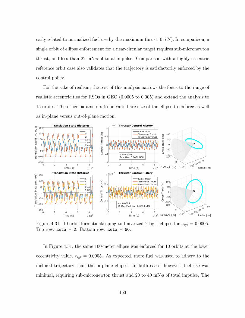
early related to normalized fuel use by the maximum thrust, 0.5 N). In comparison, a

single orbit of ellipse enforcement for a near-circular target requires sub-micronewton

thrust, and less than 22 mN·s of total impulse. Comparison with a highly-eccentric

reference orbit case also validates that the trajectory is satisfactorily enforced by the

control policy.

For the sake of realism, the rest of this analysis narrows the focus to the range of

realistic eccentricities for RSOs in GEO (0.0005 to 0.005) and extend the analysis to

15 orbits. The other parameters to be varied are size of the ellipse to enforce as well

as in-plane versus out-of-plane motion.

0 2 4 6 8

Time (s) x 105

-150

-100

-50

0

50

100

150

Tran

slat

ion S

tate

(m

, m

/s) Translation State Histories

XYZX dotY dotZ dot

0 2 4 6 8

Time (s) x 105

-1

-0.5

0

0.5

1

Con

trol

Thru

st (

N)

x 10-7 Thruster Control History

Radial ThrustTransverse ThrustCross-Track Thrust

-100100

-50

0

Cro

ss-T

rack

[m

]0

50

In-Track [m]

0

Radial [m]

-50

100

-100-150-100

e = 0.0005Fuel Use: 0.0436 NFU

0 2 4 6 8

Time (s) x 105

-150

-100

-50

0

50

100

150

Tran

slat

ion S

tate

(m

, m

/s) Translation State Histories

XYZX dotY dotZ dot

0 2 4 6 8

Time (s) x 105

-1

-0.5

0

0.5

1

Con

trol

Thru

st (

N)

x 10-7 Thruster Control History

Radial ThrustTransverse ThrustCross-Track Thrust

-100100

-50

50

0

Cro

ss-T

rack

[m

]

0

50

In-Track [m]

0

Radial [m]

-50

100

-100-150-100

e = 0.000510-Day Fuel Use: 0.0815 NFU

Figure 4.31: 10-orbit formationkeeping to linearized 2-by-1 ellipse for etgt = 0.0005.Top row: zeta = 0. Bottom row: zeta = 60.

In Figure 4.31, the same 100-meter ellipse was enforced for 10 orbits at the lower

eccentricity value, etgt = 0.0005. As expected, more fuel was used to adhere to the

inclined trajectory than the in-plane ellipse. In both cases, however, fuel use was

minimal, requiring sub-micronewton thrust and 20 to 40 mN·s of total impulse. The

153

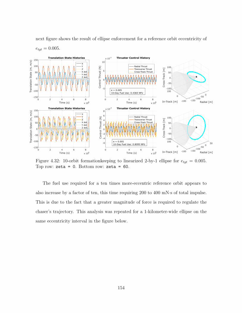
next figure shows the result of ellipse enforcement for a reference orbit eccentricity of

etgt = 0.005.

0 2 4 6 8

Time (s) x 105

-150

-100

-50

0

50

100

150

Tran

slat

ion S

tate

(m

, m

/s)

Translation State Histories

XYZX dotY dotZ dot

0 2 4 6 8

Time (s) x 105

-5

0

5

10

Con

trol

Thru

st (

N)

x 10-7 Thruster Control History

Radial ThrustTransverse ThrustCross-Track Thrust

-100100

-50

0

Cro

ss-T

rack

[m

]

0

50

In-Track [m]

0

Radial [m]

-50

100

-100-150-100

e = 0.00510-Day Fuel Use: 0.4365 NFU

0 2 4 6 8

Time (s) x 105

-150

-100

-50

0

50

100

150

Tran

slat

ion S

tate

(m

, m

/s)

Translation State Histories

XYZX dotY dotZ dot

0 2 4 6 8

Time (s) x 105

-6

-4

-2

0

2

4

6

8

Con

trol

Thru

st (

N)

x 10-7 Thruster Control History

Radial ThrustTransverse ThrustCross-Track Thrust

-100100

-50

50

0

Cro

ss-T

rack

[m

]

0

50

In-Track [m]

0

Radial [m]

-50

100

-100-150-100

e = 0.00510-Day Fuel Use: 0.8095 NFU

Figure 4.32: 10-orbit formationkeeping to linearized 2-by-1 ellipse for etgt = 0.005.Top row: zeta = 0. Bottom row: zeta = 60.

The fuel use required for a ten times more-eccentric reference orbit appears to

also increase by a factor of ten, this time requiring 200 to 400 mN·s of total impulse.

This is due to the fact that a greater magnitude of force is required to regulate the

chaser’s trajectory. This analysis was repeated for a 1-kilometer-wide ellipse on the

same eccentricity interval in the figure below.

154

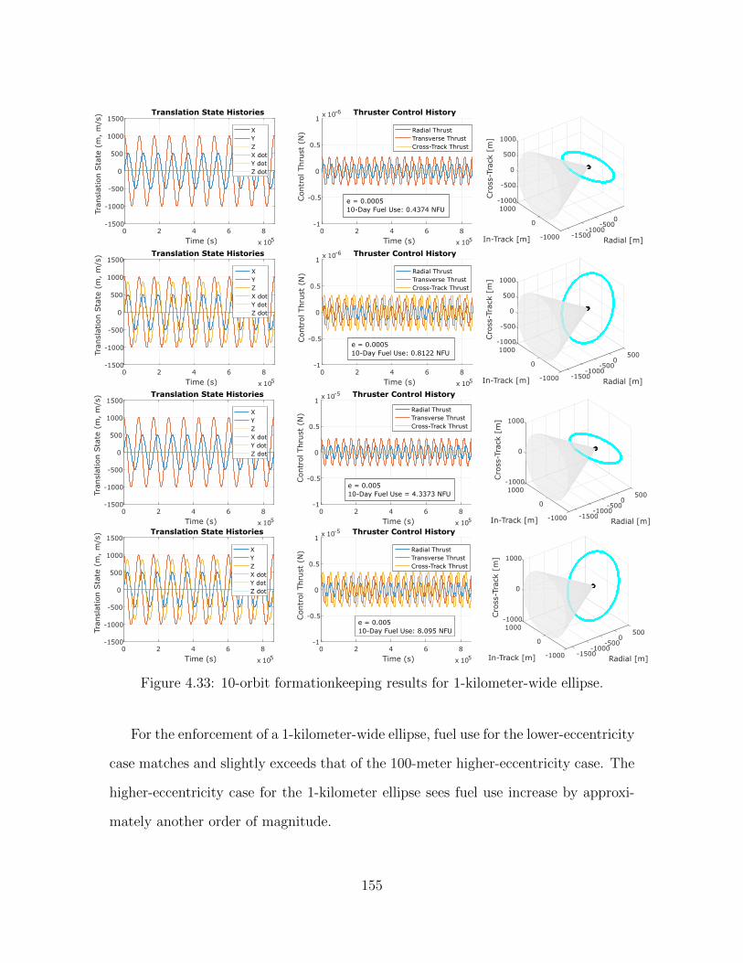
0 2 4 6 8

Time (s) x 105

-1500

-1000

-500

0

500

1000

1500

Tran

slat

ion S

tate

(m

, m

/s) Translation State Histories

XYZX dotY dotZ dot

0 2 4 6 8

Time (s) x 105

-1

-0.5

0

0.5

1

Con

trol

Thru

st (

N)

x 10-6 Thruster Control History

Radial ThrustTransverse ThrustCross-Track Thrust

-10001000

-500

0

Cro

ss-T

rack

[m

]

0

500

In-Track [m]

0

Radial [m]

-500

1000

-1000-1500-1000

e = 0.000510-Day Fuel Use: 0.4374 NFU

0 2 4 6 8

Time (s) x 105

-1500

-1000

-500

0

500

1000

1500

Tran

slat

ion S

tate

(m

, m

/s) Translation State Histories

XYZX dotY dotZ dot

0 2 4 6 8

Time (s) x 105

-1

-0.5

0

0.5

1

Con

trol

Thru

st (

N)

x 10-6 Thruster Control History

Radial ThrustTransverse ThrustCross-Track Thrust

-10001000

-500

500

0

Cro

ss-T

rack

[m

]

0

500

In-Track [m]

0

Radial [m]

-500

1000

-1000-1500-1000

e = 0.000510-Day Fuel Use: 0.8122 NFU

0 2 4 6 8

Time (s) x 105

-1500

-1000

-500

0

500

1000

1500

Tran

slat

ion S

tate

(m

, m

/s) Translation State Histories

XYZX dotY dotZ dot

0 2 4 6 8

Time (s) x 105

-1

-0.5

0

0.5

1

Con

trol

Thru

st (

N)

x 10-5 Thruster Control History

Radial ThrustTransverse ThrustCross-Track Thrust

-10001000

500

0

Cro

ss-T

rack

[m

]0

In-Track [m]

0

Radial [m]

-500

1000

-1000-1500-1000

e = 0.00510-Day Fuel Use = 4.3373 NFU

0 2 4 6 8

Time (s) x 105

-1500

-1000

-500

0

500

1000

1500

Tran

slat

ion S

tate

(m

, m

/s) Translation State Histories

XYZX dotY dotZ dot

0 2 4 6 8

Time (s) x 105

-1

-0.5

0

0.5

1

Con

trol

Thru

st (

N)

x 10-5 Thruster Control History

Radial ThrustTransverse ThrustCross-Track Thrust

-10001000

500

0

Cro

ss-T

rack

[m

]

0

In-Track [m]

0

Radial [m]

-500

1000

-1000-1500-1000

e = 0.00510-Day Fuel Use: 8.095 NFU

Figure 4.33: 10-orbit formationkeeping results for 1-kilometer-wide ellipse.

For the enforcement of a 1-kilometer-wide ellipse, fuel use for the lower-eccentricity

case matches and slightly exceeds that of the 100-meter higher-eccentricity case. The

higher-eccentricity case for the 1-kilometer ellipse sees fuel use increase by approxi-

mately another order of magnitude.

155

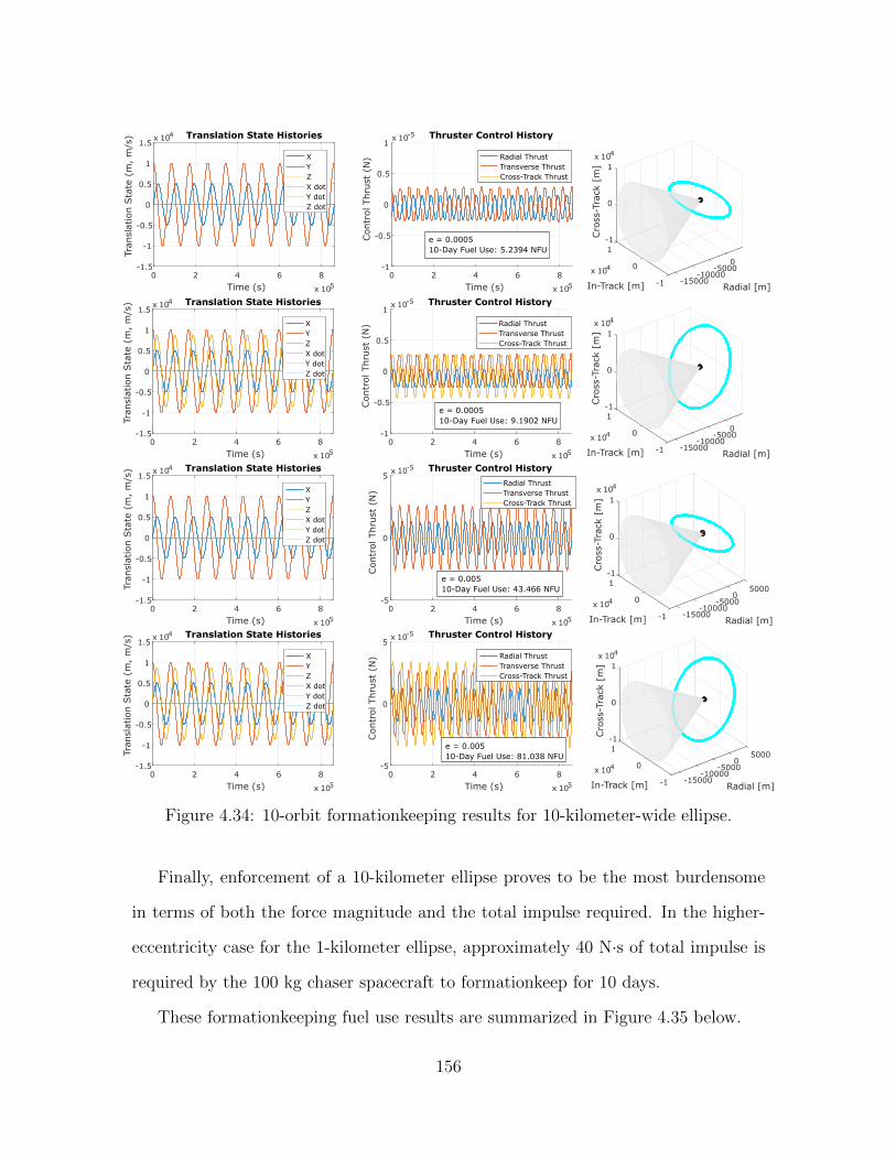
0 2 4 6 8

Time (s) x 105

-1.5

-1

-0.5

0

0.5

1

1.5

Tran

slat

ion S

tate

(m

, m

/s) x 104 Translation State Histories

XYZX dotY dotZ dot

0 2 4 6 8

Time (s) x 105

-1

-0.5

0

0.5

1

Con

trol

Thru

st (

N)

x 10-5 Thruster Control History

Radial ThrustTransverse ThrustCross-Track Thrust

-11

0

Cro

ss-T

rack

[m

]

x 104

0

In-Track [m]

x 104 0

Radial [m]

-5000

1

-10000-15000-1

e = 0.000510-Day Fuel Use: 5.2394 NFU

0 2 4 6 8

Time (s) x 105

-1.5

-1

-0.5

0

0.5

1

1.5

Tran

slat

ion S

tate

(m

, m

/s) x 104 Translation State Histories

XYZX dotY dotZ dot

0 2 4 6 8

Time (s) x 105

-1

-0.5

0

0.5

1

Con

trol

Thru

st (

N)

x 10-5 Thruster Control History

Radial ThrustTransverse ThrustCross-Track Thrust

-11

0

x 104

Cro

ss-T

rack

[m

]

0

In-Track [m]

x 104 0

Radial [m]

-5000

1

-10000-15000-1

e = 0.000510-Day Fuel Use: 9.1902 NFU

0 2 4 6 8

Time (s) x 105

-1.5

-1

-0.5

0

0.5

1

1.5

Tran

slat

ion S

tate

(m

, m

/s) x 104 Translation State Histories

XYZX dotY dotZ dot

0 2 4 6 8

Time (s) x 105

-5

0

5

Con

trol

Thru

st (

N)

x 10-5 Thruster Control History

Radial ThrustTransverse ThrustCross-Track Thrust

-11

5000

0

x 104

Cro

ss-T

rack

[m

]0

x 104

In-Track [m]

0

Radial [m]

-5000

1

-10000-15000-1

e = 0.00510-Day Fuel Use: 43.466 NFU

0 2 4 6 8

Time (s) x 105

-1.5

-1

-0.5

0

0.5

1

1.5

Tran

slat

ion S

tate

(m

, m

/s) x 104 Translation State Histories

XYZX dotY dotZ dot

0 2 4 6 8

Time (s) x 105

-5

0

5

Con

trol

Thru

st (

N)

x 10-5 Thruster Control History

Radial ThrustTransverse ThrustCross-Track Thrust

-11

5000

0

Cro

ss-T

rack

[m

]

x 104

0x 104

In-Track [m]

0

Radial [m]

-5000

1

-10000-15000-1

e = 0.00510-Day Fuel Use: 81.038 NFU

Figure 4.34: 10-orbit formationkeeping results for 10-kilometer-wide ellipse.

Finally, enforcement of a 10-kilometer ellipse proves to be the most burdensome

in terms of both the force magnitude and the total impulse required. In the higher-

eccentricity case for the 1-kilometer ellipse, approximately 40 N·s of total impulse is

required by the 100 kg chaser spacecraft to formationkeep for 10 days.

These formationkeeping fuel use results are summarized in Figure 4.35 below.

156

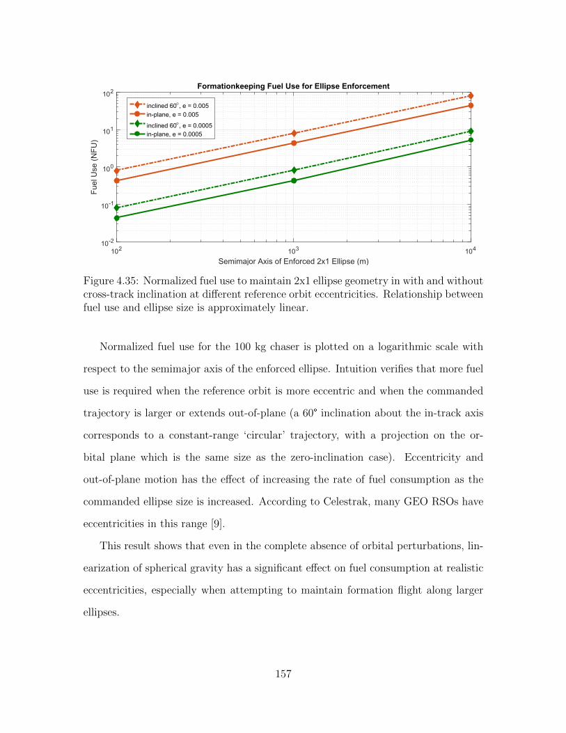
Figure 4.35: Normalized fuel use to maintain 2x1 ellipse geometry in with and withoutcross-track inclination at different reference orbit eccentricities. Relationship betweenfuel use and ellipse size is approximately linear.

Normalized fuel use for the 100 kg chaser is plotted on a logarithmic scale with

respect to the semimajor axis of the enforced ellipse. Intuition verifies that more fuel

use is required when the reference orbit is more eccentric and when the commanded

trajectory is larger or extends out-of-plane (a 60° inclination about the in-track axis

corresponds to a constant-range ‘circular’ trajectory, with a projection on the or-

bital plane which is the same size as the zero-inclination case). Eccentricity and

out-of-plane motion has the effect of increasing the rate of fuel consumption as the

commanded ellipse size is increased. According to Celestrak, many GEO RSOs have

eccentricities in this range [9].

This result shows that even in the complete absence of orbital perturbations, lin-

earization of spherical gravity has a significant effect on fuel consumption at realistic

eccentricities, especially when attempting to maintain formation flight along larger

ellipses.

157

4.5 Summary of Results

This chapter presented results from the analysis of proximity operations using the

pseudospectral collocation numerical optimization suite GPOPS-II [30] within the

contributed proximity operations analysis framework called R/POTATO.

The first section presented preliminary results on the implementation of simple

minimum-time, minimum-energy, minimum-fuel, and linear quadratic state regula-

tion in the Clohessy-Wiltshire dynamics. Solutions to these optimization problems

conformed to the expected behavior. A minimum-fuel in-track rendezvous was val-

idated mathematically for ∆V as a Hohmann phasing problem, proving that the

acceleration model and state evolution are consistent with linearized Keplerian or-

bital mechanics. The optimization performance of the tool was validated by posing

a state regulation problem with a quadratic cost function and comparing the result

with a precise simulation of full-state feedback control with an analytically-obtained

infinite-horizon LQR gain, where the error in the solution trajectory was observed to

be less than 1× 10−6 meters for a 12-hour rendezvous from hundreds of meters away.

Finally, scheduling ambiguity was shown to exist in the minimum-time problem when

thrust inputs are introduced linearly and saturate independently in each LVLH coor-

dinate (frame-component saturation), while an attitude-coupled acceleration model

for independently-saturating thrusters was shown to resolve this ambiguity and pro-

vide a more-optimal solution. The previous chapter’s claim was duly verified: an

optimal control solution with an uncoupled acceleration model is only physically con-

sistent with thruster saturation and geometry if it is assumed that a thrust-mixing

technique is used to produce the correct component forces, and that the control policy

never requires any thrusters to saturate. Such a control policy can be solutions to the

minimum-energy and control-averse LQR problems. For this reason, further analysis

158

of proximity operations were carried out using the minimum-energy objective for the

sake of reducing computational complexity.

The second section presented intermediate results, demonstrating the implementa-

tion of path constraints, phasing, endpoint constraints, and the Keplerian acceleration

model with large reference orbit eccentricity. Compliance with a geometric no-fly zone

in the shape of a 60° nadir-facing field of view cone was demonstrated for a minimum-

energy trajectory that was known to have normally violated the region. Phasing and

endpoint constraints were demonstrated in the context of a period-matching maneu-

ver for both a minimum-energy formulation (with partially satisfactory results for

an attitude-coupled minimum-time formulation provided in Appendix C). Various

24-hour minimum-energy trajectories from the same initial condition were computed

for reference orbits of various eccentricities, with major efficiency penalties only ob-

served for relatively large eccentricities (greater than 0.1). Additionally, the fact that

the shape of the control solution changes similarly to the costate as eccentricity in-

creases constitutes a qualitative validation of minimum-energy performance with the

Keplerian model.

The third section presents results from the analysis of long-duration proximity op-

erations trajectories consisting of a transfer phase and a free-orbit phase. Design of

the size, position, and orientation of the periodic trajectory was demonstrated in the

form of endpoint constraints on the terminal state of the first phase. This was first

demonstrated for Clohessy-Wiltshire dynamics and the 2-by-1 free-orbit ellipse. It was

discovered that orbit-period transfers between circumnavigating free-orbit ellipses are

relatively energy-efficient and have control policies resembling simple sinusoids that

are linearly dependent on the difference in the velocity state at corresponding angu-

lar locations on the initial and final trajectories. Implementation of simple sinusoid

control of this form results in successful ellipse phasing, but at the cost of in-track

159

offset in the destination trajectory accrued during the maneuver. R/POTATO fixes

the specified destination dynamics as the phase endpoint conditions, which avoids

this problem. Minimum-energy period matching was demonstrated under nonlinear

Keplerian relative dynamics, and it was shown that maneuvers with apogee epochs

are more fuel-efficient than maneuvers at perigee epochs as eccentricity grows. Fi-

nally, an analysis of the fuel cost of maintaining a 2-by-1 elliptical trajectory under

Keplerian relative dynamics showed that linearization has a non-trivial impact on

long-duration efficiency when realistic eccentricities are considered and when confor-

mity to kilometer-scale ellipses is enforced. These results neglect all orbital pertur-

bations, purely examining the cost of using the Clohessy Wiltshire model to linearize

Keplerian dynamics.

160

Chapter 5

Conclusions

5.1 Thesis Summary

The objective of this thesis was to explore the medium- to close-range proximity

operations problem from the standpoint of maximizing efficiency for long-duration

operations and formation flight that do not necessarily terminate in rendezvous and

docking. In the first chapter, the need for this analysis was motivated by the needs

of national defense in the orbital environment as well as the desire to maximize the

operational lifetime of future on-orbit inspection and servicing satellites.

The second chapter explored the orbital mechanics of proximity operations. It

developed the full Keplerian relative dynamics from basic kinematics, and carefully

noted each step taken to linearize and simplify them to arrive at the common Hill-

Clohessy-Wiltshire LTI dynamics and their closed-form solutions. The error asso-

ciated with this linearization was repeatedly analyzed to determine qualities such

as periodicity and magnitude at various ranges, orbital altitudes, and with small

amounts of eccentricity in the target orbit. Thrust-free periodic trajectories in the

relative frame were analyzed for both linearized and nonlinear relative dynamics,

with conditions for periodicity that can be expressed in terms of equality constraints

on the LVLH position and velocity variables. The chapter went on identify more

161

constraints which could specify the size, location, and orientation of periodic trajec-

tories in terms of the LVLH state variables; these could be obtained trigonometrically

for the Clohessy-Wiltshire 2-by-1 ellipse, but were less straightforward to obtain for

Keplerian relative trajectories. An approach using differential orbital elements and

local-frame vectors was proposed for the Keplerian case, but more work is required

to validate these. Finally, the effects of orbit perturbations on relative motion were

briefly discussed, but due to the stochastic nature of the dominating external forces,

it was determined that disturbance rejection is best dealt with using feedback control

instead of optimal control.

The third chapter introduced an optimal control formulation of the proximity op-

erations problem with an MIMO LTI thrust-saturating dynamical model. Solution

forms for problems with the common optimization objective functions minimizing

maneuver time, fuel use, and energy expenditure were developed with Pontryagin’s

Minimum Principle. The possibility of the existence of singular arcs in the prob-

lem was explored, with the conclusion that a degenerate class of singular solutions

exists for the minimum-time problem. It was determined that this was essentially

a ‘scheduling ambiguity’ that only arises when thrust control inputs are introduced

linearly and saturate independently in each coordinate, and could be mitigated in

several ways. A 13-state attitude-coupled dynamical model that respects the satura-

tion bounds of each propulsion device was introduced as one technique to resolve the

ambiguity; however, it was determined that the simpler 6-state model was still phys-

ically consistent under the assumption that thrust mixing is used and thrusters need

not saturate, as is often true in the minimum-energy problem. Last, the Rendezvous

/ Proximity Operations Trajectory Analysis Tool was introduced, and the numerical

optimization technique of GPOPS-II was briefly described and justified as a suitable

technique for obtaining smooth, energy-optimal trajectories for highly customizable

162

proximity operations problems.

The fourth chapter presented results obtained from the implementation of various

proximity operations problems in R/POTATO. Each section incrementally validated

the tool, beginning with simple rendezvous problems under various cost functions and

eventually adding nonlinear dynamics as well as path and endpoint constraints. In

the last section, transfers to specifiable Clohessy Wiltshire ellipses were demonstrated

from arbitrary initial conditions as well as from other periodic trajectories. It was

found that a class of energy-optimal trajectories for phasing between linearized el-

lipses consisted of orbit-period sinusoid control policies which result in a small amount

of in-track drift but cause the chaser to terminate along periodic trajectories. Period-

matching maneuvers subject to nonlinear Keplerian relative dynamics were demon-

strated, where an analysis with R/POTATO showed that orbit-period maneuvers are

more efficiently executed from apogee to apogee than from perigee to perigee, espe-

cially for more eccentric target orbits. Finally, the cost of linearization was revisited

for fuel use required to enforce various sizes of 2-by-1 ellipses for reference orbits with

eccentricities representative of existing RSOs in the GEO regime.

5.2 List of Contributions

The contributions made by this thesis are as follows:

A ‘cost of linearization’ analysis of the prolonged use of linearized relative dy-

namics in satellite proximity operations in terms of error in position and rate

of circumnavigation, as well as fuel use to enforce linearized trajectories.

A full list of constraints on relative position and velocities which completely

specify the size, location, and orientation of linearized periodic trajectories.

163

A proposed list of constraints on relative position and velocities to specify the

size, location, and orientation of Keplerian periodic trajectories.

An investigation of the singular class of solutions associated with the minimum-

time optimization using the 3-DOF dynamical model formulated with frame-

component saturation, accompanied by a 13-state attitude-coupled formulation

as a technique to resolve it.

A simulated demonstration of energy-optimal orbit-period simple-sinusoid con-

trol policies for uncomplicated phasing between linearized ellipses.

An analysis of energy-optimal continuous-thrust period-matching maneuvers for

both linearized and nonlinear highly-eccentric scenarios.

The Rendezvous / Proximity Operations Trajectory Analysis Tool (R/POTATO),

which can be obtained via an online repository and used with valid MATLAB

and GPOPS-II licensing.

5.3 Conclusions

The Clohessy-Wiltshire equations of relative motion were developed to be an ac-

ceptably accurate linearization of relative orbital dynamics for the terminal phases of

satellite rendezvous, where relative ranges and timescales are assumed to be small.

When conducting long-duration proximity operations for inspection and servicing of

RSOs, however, the ‘terminal phase’ may be significantly delayed or may not ever

occur. For these situations, especially at extended range and with realistic target

eccentricities, higher-fidelity relative acceleration models should be chosen instead.

Otherwise, the mission life of proximity operations platforms could be artificially

164

shortened by fuel use wasted due to the linearization of Keplerian gravity. It is im-

portant that proximity controllers use dynamics that are as consistent with nature as

possible in order to extend the mission life of formation fliers, on-orbit servicers, and

national defense assets.

It is expected that future on-orbit inspectors and servicers will make use of so-

lar electric propulsion to maximize their efficacy and lifespan. These devices exert

very low thrust over long periods of time and require prudent power management.

Best-suited to spacecraft needs in this scenario is minimum-energy optimization of

proximity operations trajectories that make use of natural thrust-free periodic motion.

This thesis does not imply that R/POTATO or GPOPS-II should be used as

an open-loop optimal trajectory planner for actual missions. Instead, they should

be used to explore the rich problem of proximity operations trajectory optimization

across multiple phases and subject to fairly complex dynamics and constraints. Gauss

pseudospectral collocation is especially useful for the types of minimum-energy opti-

mization that is apt to be carried out for future satellites equipped with solar electric

propulsion.

5.4 Future Work

5.4.1 Improvements to R/POTATO

R/POTATO stands to benefit substantially from better integration with GPOPS-

II. To start, different parts of the proximity operations problem should be scaled

appropriately based on the expected ranges of their values; for example, position

states may vary by tens of kilometers, but the endpoint constraint which matches

the chaser’s energy to the target’s must be met to high precision. Additionally,

165

better guesses and bounds can be chosen to improve the performance of the numerical

optimization.

Consideration of attitude coupling can be toggled in the Instantiation Shell, but

only limited results for small-scale minimum-time rendezvous were obtained. More

complex scenarios, such as minimum-time period-matching with an endpoint con-

straint, yielded non-ambiguous results when the cost function was reformulated to

include reaction wheel energy expenditure penalties (see Appendix C). Robust han-

dling of arbitrary initial conditions for minimum-fuel maneuvers might also be possible

with a thoughtfully structured treatment of problem phasing, but this complexity il-

lustrates why pseudospectral collocation methods are best reserved for formulations

with continuous-control solutions.

R/POTATO could also be improved as a docking simulation by enforcing end-

point constraints on the final attitude and orientation of the chaser with respect to

the target, in a similar way to that which was formulated by Boyarko, et al. This

would be relatively straightforward to accomplish for the minimum-energy case, since

the thrust-mixing assumption could allow decoupling between position and attitude

dynamics. The minimum-time case might be much more difficult to implement due

to the requirement of attitude-coupled acceleration inputs. Other docking-focused

improvements could be made, such as a requirement that the chaser refrain from con-

taminating the target with exhaust in a rendezvous scenario by enforcing off-limits

relative attitudes at close range.

Satisfaction of the Keplerian periodic trajectory specification constraints proposed

in Table 2.3 proved to be problematic for R/POTATO. More analysis to scale these

quantities correctly is likely required to obtain the desired specification control over

terminal dynamics.

R/POTATO could also be made more realistic by including perturbing effects,

166

such as J2 or third-body gravitation, in the acceleration model within the Continuous

function. Additionally, endpoint constraints aimed toward mitigating these perturba-

tions could be implemented in Endpoint (e.g., investigation of first-order J2-invariance

as described by Schaub, et al. [32] to verify the existence of Bevilacqua’s unexpected

J2-invariant inclination at 49.11° for PCO formations [4]). In theory, the dynamical

model could be made arbitrarily accurate. Effects that are purely stochastic, however,

should not be included in R/POTATO; the solver attempts to produce an end-to-end

optimal trajectory that is ideally a global minimum over a range of deterministic dy-

namics. The optimal solution inherently lacks robustness, since it must be in contact

with feasibility boundaries. Mitigation of unpredictable effects due to noisiness in the

acceleration model is better left to reference-tracking and feedback control.

5.4.2 Graphical Model Approach for On-Orbit State Estima-

tion

The assumption made in this thesis that a chaser spacecraft in GEO has full access

to its state in the LVLH frame is a significant departure from reality. Active relative

state estimation techniques such as LiDAR may be used to obtain somewhat accurate

range information, but only within close range of the target. Outside of active-range-

capable space, optical angles-only navigation can be used, but common practice is to

rely on the global state estimate provided by mean orbital element estimation from

ground station tracking. In the interest of collision avoidance, many RPO missions

limit minimum range to remain beyond a safety sphere around the target, with size

determined by the error variance of the global state estimate.

Proximity operations in LEO benefit from good access to GPS signals. Carrier-

phase differential GPS techniques can provide precise relative navigation measure-

167

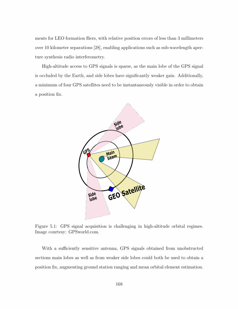
ments for LEO formation fliers, with relative position errors of less than 3 millimeters

over 10 kilometer separations [28], enabling applications such as sub-wavelength aper-

ture synthesis radio interferometry.

High-altitude access to GPS signals is sparse, as the main lobe of the GPS signal

is occluded by the Earth, and side lobes have significantly weaker gain. Additionally,

a minimum of four GPS satellites need to be instantaneously visible in order to obtain

a position fix.

Main

beam

GEO Satellite

GPS

Side lobe

Side

lobe

Figure 5.1: GPS signal acquisition is challenging in high-altitude orbital regimes.Image courtesy: GPSworld.com.

With a sufficiently sensitive antenna, GPS signals obtained from unobstructed

sections main lobes as well as from weaker side lobes could both be used to obtain a

position fix, augmenting ground station ranging and mean orbital element estimation.

168

This global estimate could be further improved by using more than one satellite.

Unlike a single monolithic chaser, a ‘chaser formation’ could cooperatively range

between themselves using LiDAR, incorporate carrier-phase differential GPS relative

state estimation, and obtain multiple independent global position estimates from the

GPS formation. The resulting joint probability distribution would have, in principle,

less error variance than a single chaser using only ground station measurements, and

could enable more ambitious proximity operations.

It is proposed that a graphical model framework be studied for incorporating

disparate types and frequencies of measurements between multiple satellites, similar

to ones described by Sanchez [31] or Setterfield [33]. This analysis should discern

whether it is feasible to perform optimal estimation of the chaser formation’s global

state in GEO, and the magnitude by which the state estimate can be improved.

169

170

Appendix A

Keplerian Orbital Mechanics

This appendix provides a brief description of fundamental orbital mechanics and

the associated equations used extensively in Chapter 2. The bulk of this material was

distilled from the texts by Vallado [38] and Bate, Mueller, and White [3]. Although

this information can be readily found in orbital mechanics textbooks, the reason it is

included here is to maintain consistency in nomenclature as well as for the reader’s

convenience.

For as long as humans have looked up at the night sky, we have been trying to

understand the motion of the orbs and lights that glide across the heavens. Aristotle

taught that these heavenly bodies, unfettered by the confines of the Earth, should

follow what was - in his mind - the only perfect natural motion: a circle. This

view went unchallenged in its basic premise for nearly two millennia; most agreed

that the planets followed circular trajectories, or combinations of circular sections.

It wasn’t until 1606 that Johannes Kepler succeeded in fitting the precise celestial

measurements of Tycho Brahe to the ellipse, and subsequently published his famous

first law in 1609: The orbit of each planet is an ellipse, with the sun at one focus.

This idea was expounded upon by Isaac Newton, who casually remarked to Edmund

Halley that if the sun pulled the planets with a force proportional to the inverse

square of their distances, their paths ought to be elliptical, and that he had written a

171

proof of it some twenty years previously. Halley pushed Newton to publish his work

in what would be known as the Principia, in what many consider to be the birth of

modern science.

Newton’s law of universal gravitation proscribes orbits to follow trajectories best

described as conic sections; usually ellipses or hyperbolae, with circles and parabolae

as respective marginally stable cases. It takes the following form when describing the

gravitational attraction between Earth and an orbiting satellite:

Fg = −Gm⊕msat

r2

(r

r

)Where m⊕ is the mass of the Earth, assumed to be much larger than the mass

of the satellite; G is the gravitational constant, also called Newton’s constant, and

is approximately equal to 6.674× 10−11m3·kg−1·s−2. The gravitational force is repre-

sented as a vector, Fg, and the distance between the Earth’s center of mass and the

satellite’s center of mass is represented as both a magnitude r and a vector r.

If the vector r can be expressed in a non-accelerating reference frame originat-

ing from the Earth’s center of mass, the following differential equation describes its

motion:

¨r = −G(m⊕ +msat)

r2

(r

r

)Of course, there is no Earth-centered reference frame that can be described as

non-accelerating or ‘inertial,’ because the Earth is itself orbiting the Sun, and thus

accelerating. The sun, too, is accelerating with respect to the center of the Milky

Way galaxy, and so on. Thus, the equation above is always an oversimplification

because it does not account for the acceleration of the reference frame in which r

is expressed. However, the period of Earth’s orbit around the sun is slow enough

172

(and the sun’s galactic orbit many orders of magnitude slower) compared to an Earth

satellite’s orbital dynamics of interest that the other, missing terms are considered to

be of negligible magnitude for pedagogical purposes.

Since the quantities G and m⊕ are constant for analysis of an Earth satellite, and

the quantity msat is so small compared to m⊕, the equation of motion is often reduced

to:

¨r = −µ⊕r2

(r

r

)Where µ⊕ represents the product Gm⊕ and is called the ‘gravitational parameter’

of Earth. This is known as the ‘Two-Body Equation of Motion,’ and is a fairly

simple representation of an orbiting body’s motion which makes several simplifying

assumptions. Summarized, they are:

The reference frame in which r is expressed is an Earth-centered and inertial

reference frame.

The ratio of the satellite’s mass to the Earth’s mass is approximately zero.

Both the satellite and the Earth are either point masses, or perfectly spherical

and uniformly dense such that they can be mathematically treated as point

masses.

There are no other external forces acting on the satellite or the Earth, to include

gravitation from a third body, no collision with particles or other momentum

transfer events, no structural heating or flexing or other mechanical energy

transfer events, etc.

It is from this equation that the six classical orbital elements (COEs), sometimes

called the six Keplerian elements, can be derived. Using these, a satellite’s orbital

173

trajectory can be fully parameterized. A brief description of each, with some useful

formulas, are provided here. For an excellent development of each of these, and as

authoritative references on basic astrodynamics in general, Vallado’s text [38] as well

as the text by Bate, Mueller, and White [3] are recommended.

A.1 The Classical Orbital Elements

Semi-major Axis. The Two-Body Equation of Motion describes an orbital tra-

jectory that can be characterized as a conic section. Every conic section is bilaterally

symmetric about two perpendicular axes, a minor axis and a major axis. For an

ellipse, which characterizes the dominant set of captured satellite orbits, the major

axis is the longer of the two; the gravitational body is located on this line at one focus

of the ellipse. The semi-major axis (a) is exactly half the length of the major axis.

Unlike the magnitude r, this parameter is constant for an orbit, and is thus a better

(yet still vague) descriptor of its ‘size.’ For a circular orbit, the semi-major axis and

the radius are equivalent. While the term ‘size’ is not descriptive enough for talking

about orbits, the semi-major axis does precisely specify a more useful quantity, the

orbit’s period:

T = 2π

√a3

µ

For circular orbits, the orbital rate n is constant and can be expressed as the

reciprocal of the orbital period T .

Another relevant quantity to mention here is the orbit’s specific mechanical energy

(ξ), a constant quantity that represents the aggregate of the satellite’s specific kinetic

energy and specific potential energy, which are constantly fluctuating between maxima

174

and minima throughout the satellite’s orbit (unless it happens to be circular). The

‘vis-viva’ equation enforces conservation of mechanical energy over the course of the

orbit:

ξ =v2

2− µ

r= − µ

2a

Eccentricity. The eccentricity of an ellipse (e) is a measure of the ‘flatness’ of

an ellipse, and varies between 0 for a circular orbit, between 0 and 1 for an elliptical

orbit, 1 for a parabolic trajectory, greater than 1 for hyperbolae, and∞ for a straight

line. Together with the semi-major axis, a more cogent understanding of an orbit’s

size can be formed. For example, the orbital radius at its smallest (periapsis, or

perigee when describing an Earth orbit) and at its largest (apoapsis or apogee) can

both be determined as follows:

rp = a(1− e)

ra = a(1 + e)

Eccentricity is also sometimes represented in vector form, emanating from the

origin of the reference frame and pointing directly toward the orbit’s periapsis. Its

magnitude is equal to the scalar value introduced above:

e =v × h

µ− r

r=

1

µ

[(v2 − µ

r

)r− (r · v)v

]While not itself an orbital element, the specific angular momentum vector

(h)

is

also an illustrative parameter of orbits. It is the cross product of the position and

velocity vectors of the orbiting satellite at any point in time, with direction parallel

to the orbit normal unit vector.

175

h = r× v

Its magnitude can also be obtained uniquely from the semi-major axis and eccen-

tricity via the semi-latus rectum, p:

p = a(1− e2) =h2

µ

∴ h =√µp

The magnitude of the satellite’s velocity can be obtained directly from its cur-

rent orbital radius and the specific mechanical energy by manipulating the vis-viva

equation:

v2 =

√2(µr

+ ξ)

=

√2(µr− µ

2a

)The angle between the velocity vector and the local horizontal (which is always

perpendicular to the radius vector) is called the flight path angle Φ.

cos Φ =h

rv

It should be noted that for elliptical orbits, the velocity’s direction is tangent to

the orbit trajectory only at perigee and apogee. For circular orbits, the satellite’s

velocity is constant and perpetually tangent to the orbit trajectory, and Φ is always

zero. Velocity has magnitude given by:

vcirc =

õ

r

Inclination. An orbit’s inclination (i) is the angle between the angular momen-

176

tum vector (or orbit normal vector) and the Earth’s north pole. This angle may vary

between 0° for an equatorial prograde orbit (orbit’s angular rate is the same sign as

Earth’s rotation rate), to 90° for a polar orbit, and 180° for an equatorial retrograde

orbit (orbit’s angular rate is the opposite sign as Earth’s rotation rate).

Right Ascension of the Ascending Node. This quantity, commonly abbrevi-

ated as RAAN or represented symbolically (Ω), is the clockwise angular displacement

of the point at which the satellite crosses from the southern hemisphere into the north-

ern hemisphere in its orbit (the ‘ascending node’) from the vernal equinox direction

(one of the axes of an Earth-centered inertial reference frame). Often, it depicted as

a vector emanating from the reference frame origin and pointing towards the orbit’s

ascending node. It may vary between 0° and 360°, but is undefined for equatorial

orbits.

Argument of Perigee. The argument of perigee (ω) is the angular displacement

from the ascending node to the orbit’s nearest approach to the gravitating body, or

periapsis, measured in the direction of the spacecraft’s motion. Together with RAAN

and inclination, the argument of perigee fully describes the orientation of the orbital

trajectory in 3-dimensional space.

True Anomaly. This quantity is the angular displacement of the satellite’s

position along its orbital trajectory from the orbit’s perigee, also measured in the

direction of the satellite’s motion. It is written symbolically in a number of ways by

different authors, but in this thesis, it will be denoted by ν. This final orbital element

places the satellite itself unambiguously at a point in 3-dimensional space along its

trajectory. With this quantity, along with the semi-major axis and eccentricity, the

satellite’s instantaneous orbit radius magnitude can be determined using the following

formula:

177

r =p

1 + e cos(ν)

The magnitude of the derivative of the radius vector can also be expressed as a

function of true anomaly:

r =rνe sin ν

1 + e cos ν

It is important to note that this quantity is not equivalent to the magnitude of the

velocity vector, however. The expression requires the time derivative of true anomaly,

which is:

ν =h

r2

We can use both r and ν to differentiate true anomaly again while simplifying:

ν =−2rν

r=

−2h2e sin ν

r4(1 + e cos ν)

A.2 Describing Angular Motion

Since all captured orbits can be described as ellipses, it is useful to be able to

describe locations of objects on elliptical trajectories. The equation in cartesian

coordinates of any ellipse centered at (x0, y0) is given by:

(x− x0)2a2

+(y − y0)2

b2= 1

Where the quantities a and b represent the lengths of the semi-major and the

semi-minor axes, respectively. The area of the entire ellipse is given by the product

178

ab. The ratio of the semi-minor axis to the semi-major axis is also related to the

eccentricity of the ellipse as follows:

√1− e2 =

b

a

Determining the time-of-flight of an object in an eccentric orbit requires a multi-

step computation that takes no fewer than three angular parameters into account:

true anomaly (ν, which was described above and can be obtained from an instan-

taneous orbit radius measurement for an orbit of known period and eccentricity),

eccentric anomaly (E), and mean anomaly (M). The true anomaly is the angular

measure from the periapsis vector to the orbit radius vector, and thus the vertex of

the angle is situated at a major focus of the ellipse. Eccentric anomaly, however, is

an angle with its vertex at the ellipse’s center; it requires the circumscription of an

auxiliary circle with radius equal to the orbit’s semi-major axis. Eccentric anomaly is

the angle of a point on the auxiliary circle that is collinear with the satellite’s position

on a line perpendicular to the major axis of the ellipse. It can be determined from

true anomaly and eccentricity using the following equation:

cos (ν) =cos (E)− e

1− e cos (E)

Mean anomaly is the one-to-one matching of two ratios: the amount of time

elapsed since periapsis to the duration of the orbital period, and a fraction of 2π.

Mean anomaly is always constant over the course of any orbit. It is given by:

M = n(t− t0)

Where t0 is the time at perigee, and n is the ‘mean motion,’ or average angular

179

rate, of the orbit:

n =

õ

a3

Using Kepler’s Second Law, which states that objects in orbit sweep out equal

areas in equal times, the following geometric relationship can be obtained between

mean anomaly and eccentric anomaly:

M = E − e sin (E)

While mean anomaly can be obtained from eccentric anomaly in one step, de-

termining eccentric anomaly from mean anomaly requires the use of an iterative

numerical root-finding technique such as the Newton-Raphson method. It is typical

to provide the current mean anomaly as an “initial guess” for these root-finding al-

gorithms, since it is close in value to eccentric anomaly for orbits of relatively small

eccentricity.

A.3 Orbital Perturbations

As was alluded to above, what is gained in the mathematical simplicity of the Two-

Body Equation of Motion is lost from the realism of an actual Earth satellite’s motion.

While the Two-Body Equation is useful in defining the ideal conic section trajectory

of an orbit, true orbits experience various perturbations (basically, external forces)

which alter certain parameters of its orbit in different ways. These disturbances are

often time-varying, difficult to predict and measure, and can be periodic or secular

in nature. Some of the most prominent perturbations, as well as how they affect an

orbit (encoded as changes in the orbital elements) are described here. In general, these

180

descriptions follow from the texts of Vallado [38] and Bate, Mueller, and White [3].

Drag. A discrete transition between the Earth’s atmosphere below and the vac-

uum of space above does not exist. Instead, the transition is gradual. For this reason,

Earth satellites experience a slight air drag force which acts in a direction opposite

to the orbit velocity vector. The force of air drag is increased as a satellite descends

lower in its orbit toward the Earth, and also increases with the cross-sectional surface

area of the satellite. The effect that drag has on orbits is to reduce the semi-major

axis and the eccentricity. The intuition for this comes from imagining the effect

of reducing the maximum kinetic energy of the satellite as it flies through perigee;

this causes the total mechanical energy of the orbit to fall, which is taken from the

maximum potential energy at apogee.

Oblate Earth (J2). The Earth’s oblateness refers to the equatorial bulge of

the planet. The planet’s radius at the equator is 21 kilometers larger than its polar

radii, which is likely due to centrifugal flexion over its lifetime. One effect that this

has on orbits is to ‘pull down’ their inclination, making them closer to equatorial.

This effect can be imagined by considering the gravitational torque that the extra

equatorial mass exerts on the satellite as it passes through its maximum and minimum

latitudes [3]. This torque in turn causes the orbit to precess, acting the same way

a top or a gyroscope would under the exertion of a similar torque. This precession

causes the ascending node to move westward with respect to the Earth, and is called

‘nodal regression.’ The magnitude of nodal regression decreases with altitude. A

third effect of Earth’s oblateness is ‘apsidal rotation,’ which describes the rotation of

the major axis of an eccentric orbit in the direction of motion of the satellite; it is a

function of orbital altitude, eccentricity, and inclination. Interestingly, orbits with an

inclination of exactly 63.4° experience no apsidal rotation, as this is the point along

the continuum of inclinations at which the apsidal rotation effect changes sign.

181

Third Body Effects. Gravitation due to other celestial bodies, such as from

Earth’s moon and the sun, have a non-negligible effect on satellites. Unlike drag and

oblate Earth effects, which are secular, third body effects become more dramatic at

higher altitudes, and are non-secular. However, this periodicity does not make it easy

to analyze or plan for; these effects are often treated stochastically. In interplane-

tary missions, orbit propagators increase the granularity of their computations as a

trajectory nears other attracting bodies.

Photon Pressure. Satellites that have a low mass-to-area ratio are especially

susceptible to momentum transfer from solar radiation. Although photons are mass-

less particles, they still impart momentum on incident surfaces, whether they are

reflected or absorbed. This perturbation is also non-secular, and the magnitude of

the disturbance force depends on the surface properties of the satellite. The direction

of the force, however, varies with orbital period, as would be expected.

Other Perturbations. There are several other perturbative forces which af-

fect satellites, including interaction with Earth’s magnetic field, momentum transfer

from thrusters or out-gassing substances, relativistic effects, and zonal and sectorial

harmonic irregularities of the distribution of Earth’s mass, to name a few. Though

not explicitly associated with orbit-changing perturbations, gravitational tidal forces

cause satellites to torque until their major body axis aligns with the radius vector,

often called ‘gravity gradient’ torque.

182

Appendix B

Nonlinear Solver Error Analysis

This appendix details the choice of nonlinear solver used to integrate the full

nonlinear equations of relative motion and produce the results from Chapter 2, and

an analysis of its accuracy compared to results from AGI’s Systems Tool Kit (formerly

Satellite Tool Kit) [36]. Unlike GPOPS-II, this solver is a built-in MATLAB function,

so these results can be reproduced using only a standard MATLAB license.

For tolerances, the quantity eps is used. Due to limited floating-point resolution

in MATLAB, there is no double-precision number between 1 and (1+eps). Thus, it

is not useful to specify absolute tolerance any smaller than the quantity eps, here

denoted ε, which is equal to 2.2204e-16. Relative tolerance is set to the lowest value

permitted by ode113 given the absolute tolerance.

The following statistics are produced for both ode113 and ode45 using the same

tolerances when attempting to numerically integrate the nonlinear Keplerian equa-

tions of relative motion for the 10-orbit, arbitrary initial condition problem from

Chapter 2. The solutions from both solvers were found to agree to within a frac-

tion of a millimeter. In comparison, ode113 obtains the solutions with the desired

precision faster and with fewer function evaluations. According to the MATLAB doc-

umentation, ode113 is better at solving problems with both smooth solution curves

and stringent error tolerances, as commonly occur in orbital dynamics problems.

183

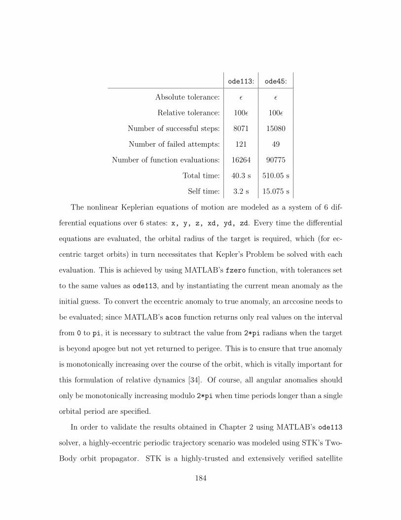
ode113: ode45:

Absolute tolerance: ε ε

Relative tolerance: 100ε 100ε

Number of successful steps: 8071 15080

Number of failed attempts: 121 49

Number of function evaluations: 16264 90775

Total time: 40.3 s 510.05 s

Self time: 3.2 s 15.075 s

The nonlinear Keplerian equations of motion are modeled as a system of 6 dif-

ferential equations over 6 states: x, y, z, xd, yd, zd. Every time the differential

equations are evaluated, the orbital radius of the target is required, which (for ec-

centric target orbits) in turn necessitates that Kepler’s Problem be solved with each

evaluation. This is achieved by using MATLAB’s fzero function, with tolerances set

to the same values as ode113, and by instantiating the current mean anomaly as the

initial guess. To convert the eccentric anomaly to true anomaly, an arccosine needs to

be evaluated; since MATLAB’s acos function returns only real values on the interval

from 0 to pi, it is necessary to subtract the value from 2*pi radians when the target

is beyond apogee but not yet returned to perigee. This is to ensure that true anomaly

is monotonically increasing over the course of the orbit, which is vitally important for

this formulation of relative dynamics [34]. Of course, all angular anomalies should

only be monotonically increasing modulo 2*pi when time periods longer than a single

orbital period are specified.

In order to validate the results obtained in Chapter 2 using MATLAB’s ode113

solver, a highly-eccentric periodic trajectory scenario was modeled using STK’s Two-

Body orbit propagator. STK is a highly-trusted and extensively verified satellite

184

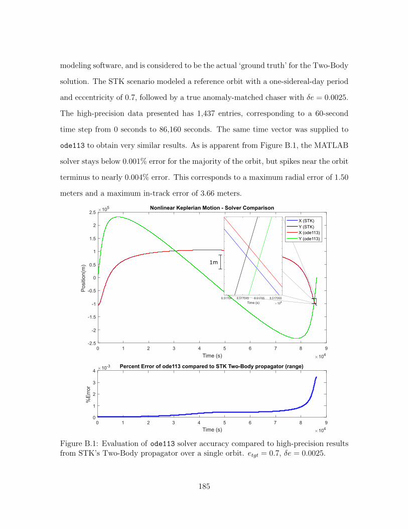
modeling software, and is considered to be the actual ‘ground truth’ for the Two-Body

solution. The STK scenario modeled a reference orbit with a one-sidereal-day period

and eccentricity of 0.7, followed by a true anomaly-matched chaser with δe = 0.0025.

The high-precision data presented has 1,437 entries, corresponding to a 60-second

time step from 0 seconds to 86,160 seconds. The same time vector was supplied to

ode113 to obtain very similar results. As is apparent from Figure B.1, the MATLAB

solver stays below 0.001% error for the majority of the orbit, but spikes near the orbit

terminus to nearly 0.004% error. This corresponds to a maximum radial error of 1.50

meters and a maximum in-track error of 3.66 meters.

0 1 2 3 4 5 6 7 8 9

Time (s) 104

0

1

2

3

4

%E

rro

r

10-3 Percent Error of ode113 compared to STK Two-Body propagator (range)

0 1 2 3 4 5 6 7 8 9

Time (s) 104

-2.5

-2

-1.5

-1

-0.5

0

0.5

1

1.5

2

2.5

Pos

ition

(m)

105 Nonlinear Keplerian Motion - Solver Comparison

8.51704 8.517045 8.51705 8.517055

Time (s) 104

1m

X (STK)

Y (STK)X (ode113)

Y (ode113)

Figure B.1: Evaluation of ode113 solver accuracy compared to high-precision resultsfrom STK’s Two-Body propagator over a single orbit. etgt = 0.7, δe = 0.0025.

185

To investigate the error spike from the propagation of a single orbit, the same

comparison was extended to ten orbits with the same step size. The result is shown

in Figure B.2 below: range error spikes periodically around orbit perigee, where the

states are evolving quickly. Also, the baseline error slowly grows over time, with a

small bump in error at apogee beginning to form. Interestingly, there is an error spike

associated with every perigee except the initial one (at time t = 0), which seems to

further indicate that the discrepancy is primarily attributable to propagation. At the

end of ten orbits in this highly-eccentric reference orbit, absolute range error stays

belows 0.04%, the maximum radial error was 14.89 meters, and the maximum in-track

error was 36.55 meters.

0 1 2 3 4 5 6 7 8 9

Time (s) 105

-2.5

-2

-1.5

-1

-0.5

0

0.5

1

1.5

2

2.5

Pos

ition

(m

)

105 Nonlinear Keplerian Motion - Solver Comparison (10 orbits)

0 1 2 3 4 5 6 7 8 9

Time (s) 105

0

0.01

0.02

0.03

0.04

%E

rro

r

Percent Error of ode113 compared to STK Two-Body propagator (range) (10 orbits)

Figure B.2: Evaluation of ode113 solver accuracy compared to high-precision resultsfrom STK’s Two-Body propagator over ten orbits. etgt = 0.7, δe = 0.0025.

186

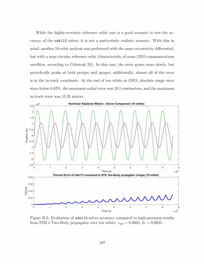
While the highly-eccentric reference orbit case is a good scenario to test the ac-

curacy of the ode113 solver, it is not a particularly realistic scenario. With this in

mind, another 10-orbit analysis was performed with the same eccentricity differential,

but with a near-circular reference orbit (characteristic of some GEO communications

satellites, according to Celestrak [9]). In this case, the error grows more slowly, but

periodically peaks at both perigee and apogee; additionally, almost all of the error

is in the in-track coordinate. At the end of ten orbits at GEO, absolute range error

stays below 0.02%, the maximum radial error was 19.1 centimeters, and the maximum

in-track error was 15.33 meters.

0 1 2 3 4 5 6 7 8 9

Time (s) 105

-2.5

-2

-1.5

-1

-0.5

0

0.5

1

1.5

2

2.5

Pos

ition

(m

)

105 Nonlinear Keplerian Motion - Solver Comparison (10 orbits)

0 1 2 3 4 5 6 7 8 9

Time (s) 105

0

0.01

0.02

0.03

0.04

%E

rro

r

Percent Error of ode113 compared to STK Two-Body propagator (range) (10 orbits)

Figure B.3: Evaluation of ode113 solver accuracy compared to high-precision resultsfrom STK’s Two-Body propagator over ten orbits. etgt = 0.0005, δe = 0.0025.

187

The following MATLAB function demonstrates how ode113 was used to produce

the results in Chapter 2.

1 function ProxOpsDemo()2 % This function is a demonstration of how to obtain3 % high-precision relative orbital trajectories using4 % MALTAB's ode113 solver to integrate the nonlinear5 % Two-Body Keplerian dynamics describing relative motion.6 % Z. Funke, 20177

8 clear yd0;9 syms yd0;

10

11 Re = 6378.137 * 1000; % Earth's mean equatorial radius [m]12 mu = 3.986004419e14; % Earth's grav. parameter [mˆ3/sˆ2]13 alt GEO = 35786 * 1000; % GEO altitude [m]14 alt LEO = 200 * 1000; % LEO altitude [m]15 alt ISS = 400 * 1000; % ISS altitude [m]16

17 % Begin user-modifiable section -------------------------------------18 a = Re + alt GEO; % Reference orbit semimajor axis [m]19 e = 0.7; % Reference orbit eccentricity20 t0 = 0; % Target's time ahead of perigee [s]21 de = 0.0025; % Differential eccentricity of chaser22 % Set y0 = 0 for target-centered trajectory.23 y0 = 0.5*a*de; % Initial in-track position of chaser24 % Set z0 = zd0 = 0 for coplanar trajectory.25 z0 = -0.5*a*de; % Initial cross-track pos of chaser26 zd0 = 20; % Initial cross-track vel of chaser27 num orbits = 1; % Number of orbits to propagate28 % End user-modifiable section --------------------------------------29

30 n = sqrt(mu/(aˆ3)); % Target mean motion31 P = 2*pi/n; % Target period32 tspan = [0 num orbits*P]; % Solver timespan33

34 % Instantiate target based on t0 by solving Kepler's Problem35 M 0 = mod(n*t0,2*pi);36 E 0 = fzero(@(E 0) E 0-e*sin(E 0)-M 0, M 0, ...37 optimset('Display','off','TolFun',eps,'TolX',eps));38 if E 0 < pi39 nu 0 = acos((cos(E 0)-e)/(1-e*cos(E 0)));40 else41 nu 0 = 2*pi - acos((cos(E 0)-e)/(1-e*cos(E 0)));42 end%if43 r tgt 0 = (a*(1-eˆ2))/(1+e*cos(nu 0));44 h tgt = sqrt(mu * a*(1-eˆ2));45 nu dot 0 = h tgt/(r tgt 0ˆ2);

188

46 nu ddot 0 = (-2*h tgtˆ2*e*sin(nu 0))/(r tgt 0ˆ4*(1+e*cos(nu 0)));47 rd tgt 0 = (r tgt 0*nu dot 0*e*sin(nu 0))/(1+e*cos(nu 0));48

49 % Chaser's initial position50 x0 = -a*de;51 %y0 set by user52 %zo set by user53 xd0 = 0;54 %yd0 set below to match energy55 %zd0 set by user56

57 r ch 0 = sqrt((r tgt 0+x0)ˆ2 + y0ˆ2 + z0ˆ2);58 % Solve vis-viva equation for yd0 that matches orbit energies59 yd0s = vpa(solve(-mu/(2*a) == ...60 0.5*((rd tgt 0 + xd0-nu dot 0*y0)ˆ2 + ...

(yd0+nu dot 0*(r tgt 0+x0))ˆ2 + zd0ˆ2) - mu/r ch 0,yd0));61 yd0 = double(yd0s(2));62

63 ICs = [x0; y0; z0; xd0; yd0; zd0];64

65 % Call ode113 nonlinear solver66 options = odeset('RelTol',1e2*eps,'AbsTol',eps, 'Stats','on');67 [T OUT,SOL OUT] = ode113(@Kepler fun,tspan, ICs,options);68 X NLEM = SOL OUT(:,1);69 Y NLEM = SOL OUT(:,2);70 Z NLEM = SOL OUT(:,3);71 XD NLEM = SOL OUT(:,4);72 YD NLEM = SOL OUT(:,5);73 ZD NLEM = SOL OUT(:,6);74

75 %---------- ODE function ---------76 function OUT = Kepler fun(t,input)77 x = input(1);78 y = input(2);79 z = input(3);80 xd = input(4);81 yd = input(5);82 zd = input(6);83 M = mod(n*(t + t0),2*pi);84 E = fzero(@(E) E-e*sin(E)-M, M, ...85 optimset('Display','off','TolFun',eps,'TolX',eps));86 if E < pi87 nu = acos((cos(E)-e)/(1-e*cos(E)));88 else89 nu = 2*pi - acos((cos(E)-e)/(1-e*cos(E)));90 end%if91 r tgt = (a*(1-eˆ2))/(1+e*cos(nu));92 nu dot = h tgt/(r tgtˆ2);93 rd tgt = (r tgt*nu dot*e*sin(nu))/(1+e*cos(nu));94 nu ddot = -2*rd tgt*nu dot/(r tgt);95 r ch = sqrt((r tgt+x)ˆ2 + yˆ2 + zˆ2);

189

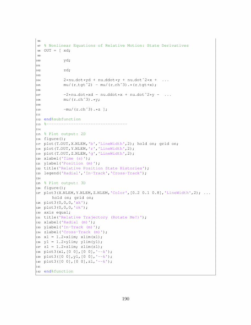
96

97 % Nonlinear Equations of Relative Motion: State Derivatives98 OUT = [ xd;99

100 yd;101

102 zd;103

104 2*nu dot*yd + nu ddot*y + nu dotˆ2*x + ...105 mu/(r tgtˆ2) - mu/(r chˆ3).*(r tgt+x);106

107 -2*nu dot*xd - nu ddot*x + nu dotˆ2*y - ...108 mu/(r chˆ3).*y;109

110 -mu/(r chˆ3).*z ];111

112 end%subfunction113 %---------------------------------114

115 % Plot output: 2D116 figure();117 plot(T OUT,X NLEM,'b','LineWidth',2); hold on; grid on;118 plot(T OUT,Y NLEM,'r','LineWidth',2);119 plot(T OUT,Z NLEM,'g','LineWidth',2);120 xlabel('Time (s)');121 ylabel('Position (m)');122 title('Relative Position State Histories');123 legend('Radial','In-Track','Cross-Track');124

125 % Plot output: 3D126 figure();127 plot3(X NLEM,Y NLEM,Z NLEM,'Color',[0.2 0.1 0.8],'LineWidth',2); ...

hold on; grid on;128 plot3(0,0,0,'xk');129 plot3(0,0,0,'ok');130 axis equal;131 title('Relative Trajectory (Rotate Me!)');132 xlabel('Radial (m)');133 ylabel('In-Track (m)');134 zlabel('Cross-Track (m)');135 xl = 1.2*xlim; xlim(xl);136 yl = 1.2*ylim; ylim(yl);137 zl = 1.2*zlim; zlim(zl);138 plot3(xl,[0 0],[0 0],'--k');139 plot3([0 0],yl,[0 0],'--k');140 plot3([0 0],[0 0],zl,'--k');141

142 end%function

190

Appendix C

Quaternion Convention

C.1 Quaternion Convention for R/POTATO

Many aerospace systems use quaternions to describe attitude for a variety of

reasons. Unlike roll-pitch-yaw attitude interpretations, quaternions are continuous

and avoid problems such as gimbal-lock. Also, it is computationally straightforward to

calculate transformations with them and to propagate them over time. Additionally,

their dynamics are continuous and devoid of singularities. However, whenever using

quaternions it is essential to clearly describe which convention is used, as there are

various in common use.

A quaternion is a mathematical representation of a three dimensional orientation

and is comprised of both a three-dimensional vector part and one scalar component,

as shown below.

q =

~qq4

=

q1

q2

q3

q4

The convention used in this thesis is to place the vector component along the first

191

three elements of the quaternion and the scalar component as the fourth and final

element. When representing attitude, the unit quaternion is always used, such that

the norm |q| =√

q21 + q2

2 + q23 + q2

4 = 1. In essence, the quaternion is a rotation

operator that specifies the rotation of one reference frame to another. Though quater-

nions are somewhat less intuitive than roll-pitch-yaw angles to visualize, the easiest

way to understand them is to consider the rotation from one frame to the other as a

single rotation about some Euler axis (a three-dimensional unit vector). This can be

represented mathematically as follows:

q =

~e sin(θ/2)

cos(θ/2)

where e is the unit Euler axis and θ is the angle of rotation about the Euler axis

to rotate from one frame to the other.

There are at least twelve different ways to define a quaternion convention (hence the

dedication of an appendix to a thorough explanation). They are differentiated from

one another by answering the following questions:

Scalar component is first or last?

Coordinate system is left-handed or right-handed?

Quaternion operation is active (alibi) or passive (alias)?

if passive, quaternion transforms global-to-local or local-to-global?

It was mentioned previously that the convention in use places the scalar compo-

nent last in the quaternion. Like most quaternion conventions, this thesis uses a

right-handed coordinate system (though there are notable exceptions, such as the Jet

Propulsion Laboratory who use a left-handed convention for visual-inertial odometry,

192

SLAM, etc. [35]).

R/POTATO uses a ‘passive’ interpretation of the quaternion operator, which is

the most nuanced concept to understand about quaternion conventions. Often, this

is referred to as the ‘function’ of the quaternion operator: whether it performs a

rotation (active) or a transformation (passive). Mathematically, this function is the

following operation:

q⊗ v ⊗ q∗

That is, if q is an active quaternion, the vector v is rotated into a new reference frame;

on the other hand, if the quaternion is passive, the vector v is resolved into a new

reference frame. The above formula can be thought of as the ‘default operation’ of the

quaternion. To perform this operation, it is important to realize that the ⊗ operator

denotes quaternion multiplication, q∗ denotes the conjugate of the quaternion, and

the vector v must be represented as a 4-vector v by appending a zero where the scalar

component of a quaternion would be located (however, it is not necessary that v be

normalized). To illustrate the difference, consider being an inertially-fixed observer

looking at the 3-vector v. It has three components expressed in some reference frame

called A. There is some other reference frame of interest, B, that is oriented differently

than A. Then, there is an active quaternion q which rotates v from A to B, where

it is now a completely different vector w. To you, the vector’s orientation appears

to have actively changed. Contrast this with a vector transformation, where the

main difference is that the vector v would not appear to change at all. Instead, the

transformation simply assigns new component magnitudes to v based on its position

with respect to B instead of A; in effect, the vector vA is simply renamed to vB. A

good visualization of this description is shown in Figure 1A on the next page. Another

way to describe the difference between active and passive rotation is to simply say

193

that an active quaternion rotates the vector, whereas a passive quaternion rotates

the reference frame. These are effectively opposite actions. Thus, active and passive

quaternions are complex conjugates of each other (they denote rotations of opposite

signs about the same axis). Note that if both the vector and the frame are rotated,

this ‘undoes’ the operation; the resulting vector has the same components in Frame

B as it did in Frame A, and there is no longer a relationship between the frames.

xA

yA

zA

xB

yB

zB

Coordinate Frame A Coordinate Frame B

xA

yA

zA

vA

wA wB

xB

yB

zB

vB

Vector vA in Frame A Vector vB in Frame B

xA

yA

zA

xB

yB

zB

Vector wA in Frame A Vector wB in Frame B

Figure C.1: The difference between vector rotation (lower left) and vector resolution(middle right). If both are performed (lower right), the result is not meaningful whencompared to the original (middle left).

For a more in-depth discussion of active and passive rotations, further explanation

accompanied with examples can be found in Karsten’s paper. [15]

194

For completeness, it should also be mentioned that quaternion representations

are a so-called ‘double-cover’ of attitude, meaning that for every possible orientation,

there are exactly two distinct quaternions that describe it: namely q and −q. Simu-

lations, software, and kinematic propagators make no preference for one or the other.

However, −q is not to be confused with the quaternion conjugate q∗, in which only

the vector part is negated; the conjugate does correspond with a different rotation,

specifically the rotation opposite that described by q.

The kinematic equation for propagating quaternions is a function of the angular

rate of both the body and the global frames. For the convention used in this thesis,

it is:

q =1

2(q⊗ ωL − ωG ⊗ q) (5A)

Where ωL and ωG are the angular rate vectors of the local and global reference

frames, respectively, and are quaternion-multiplied by appending a zero in the scalar

position. The global rate vector is often taken to be zero for many formulations, in

which case the equation assumes its more commonly-seen form where the second term

is omitted. A word of caution: this equation may change when different conventions

are used. The other forms are given in [13]. Unfortunately, many of the differences in

quaternion conventions amount to simple inversions due to individual differences such

as passive or active function, and much confusion can arise when even numbers of

these inversions make two very different interpretations behave in a mathematically

identical fashion. The best policy is to always thoroughly understand the convention

in use and validate it in as many ways as needed to resolve any ambiguity.

An excellent and comprehensive reference on quaternions, conventions for using

them, and describing attitude kinematics with them can be found in [35].

195

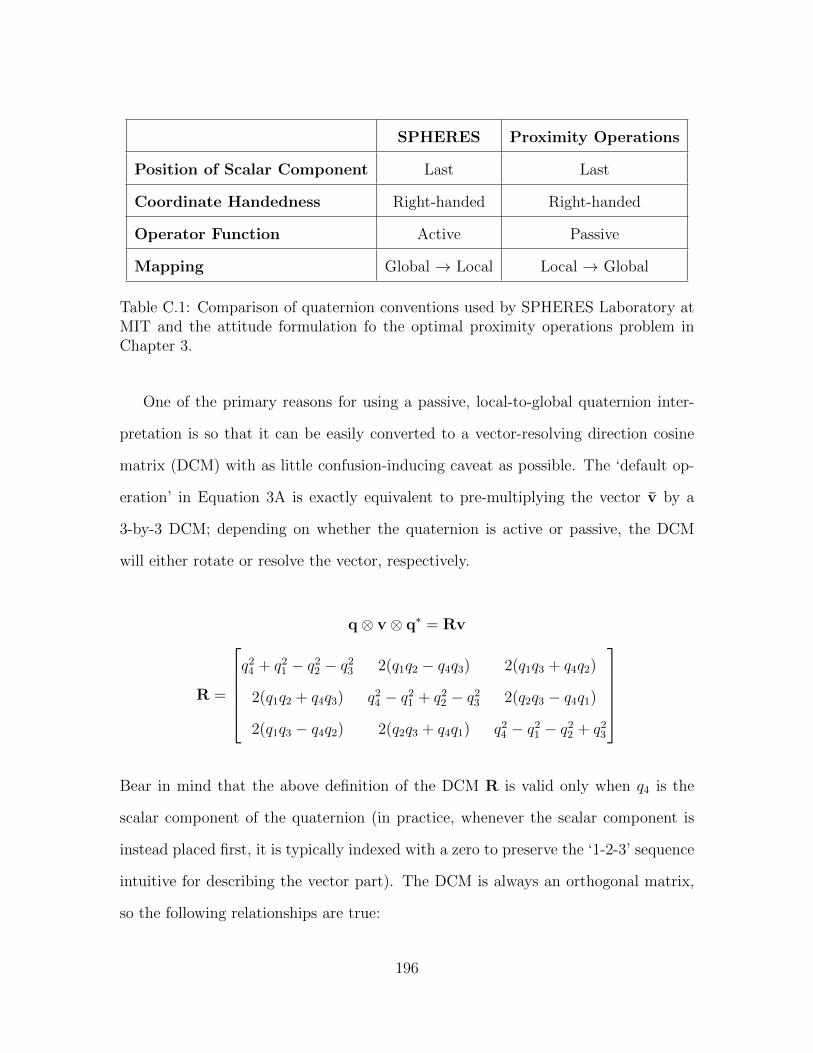
SPHERES Proximity Operations

Position of Scalar Component Last Last

Coordinate Handedness Right-handed Right-handed

Operator Function Active Passive

Mapping Global → Local Local → Global

Table C.1: Comparison of quaternion conventions used by SPHERES Laboratory atMIT and the attitude formulation fo the optimal proximity operations problem inChapter 3.

One of the primary reasons for using a passive, local-to-global quaternion inter-

pretation is so that it can be easily converted to a vector-resolving direction cosine

matrix (DCM) with as little confusion-inducing caveat as possible. The ‘default op-

eration’ in Equation 3A is exactly equivalent to pre-multiplying the vector v by a

3-by-3 DCM; depending on whether the quaternion is active or passive, the DCM

will either rotate or resolve the vector, respectively.

q⊗ v ⊗ q∗ = Rv

R =

q24 + q21 − q22 − q23 2(q1q2 − q4q3) 2(q1q3 + q4q2)

2(q1q2 + q4q3) q24 − q21 + q22 − q23 2(q2q3 − q4q1)

2(q1q3 − q4q2) 2(q2q3 + q4q1) q24 − q21 − q22 + q23

Bear in mind that the above definition of the DCM R is valid only when q4 is the

scalar component of the quaternion (in practice, whenever the scalar component is

instead placed first, it is typically indexed with a zero to preserve the ‘1-2-3’ sequence

intuitive for describing the vector part). The DCM is always an orthogonal matrix,

so the following relationships are true:

196

qactive = q∗passive

Ractive = R−1passive = RTpassive

So, the fact that the quaternion used for proximity operations is ‘passive’ and

‘local-to-global’ means that it will resolve a body-frame vector into the LVLH frame

when that vector is pre-multiplied by the DCM. This interpretation is straightforward

for describing the dynamics of the attitude-coupled problem, where it is important

to resolve the chaser’s thrust vector into the LVLH reference frame.

The quaternion product with the angular rate vector in the quaternion kinematic

equation is more commonly expressed as a matrix product between a skew-symmetric

4-by-4 matrix and the quaternion. This skew-symmetric matrix may take one of two

forms, depending on whether there needs to be a pre- or post-multiplication of angular

rate in the quaternion product. For clarity, both forms are shown below.

Pre-Multiplying Post-Multiplying

by Angular Rate by Angular Rate

12ω ⊗ q 1

2q⊗ ω

= 12Ωpreq = 1

2Ωpostq

Ωpre =

0 −ω3 ω2 ω1

ω3 0 −ω1 ω2

−ω2 ω1 0 ω3

−ω1 −ω2 −ω3 0

Ωpost =

0 ω3 −ω2 ω1

−ω3 0 ω1 ω2

ω2 −ω1 0 ω3

−ω1 −ω2 −ω3 0

Table C.2: Comparison of skew-symmetric angular rate matrices for quaternion kine-matics, differing based on ordering of the quaternion product.

197

C.2 Partial Results from Minimum-Time Period

Matching

The intermediate results section of Chapter 4 explored the optimal period-matching

results for a fixed-final-time minimum-energy objective function. This section presents

partial results from the implementation of an attitude-coupled minimum-time period

matching maneuver. Because the minimum-time result is desired, it is necessary to

use the attitude-coupled acceleration model to respect thruster saturation. The re-

sult of the attitude-coupled minimum-time period matching analysis is shown in the

figures below, and was obtained by setting InclAttDynamics = 1 and MinTime = 1

along with PeriodMatch = 1.

In Figure C.2, the objective function used is J =∫ tft0

1 dt. The result is unex-

pected because the thruster does not execute extremal control, instead staying nearly

constant at an intermediate value. The reaction wheels appear to re-orient the thrust

vector in a half-rotation over the course of the thrusting phase. However, the reaction

wheel torque history exhibits ‘singular-like’ behavior similar to the previous control

solutions which contained ambiguity. This result is more likely the result of an ill-

posed problem than solver error.

198

0 2 4 6 8

Time (s) x 104

-6000

-4000

-2000

0

2000

Tran

slat

ion S

tate

(m

, m

/s) Translation State Histories

XYZX dotY dotZ dot

0 2 4 6 8

Time (s) x 104

-1

-0.5

0

0.5

1

Quat

ernio

n M

agnitude

Quaternion Histories

q1q2q3q4Phase

0 2 4 6 8

Time (s) x 104

-1

-0.5

0

0.5

1

Rot

atio

n R

ates

(ra

d/s

)

Rotation Rate Histories

wxwywzPhase Boundary

0 2 4 6 8

Time (s) x 104

0

0.1

0.2

0.3

0.4

0.5

Con

trol

Thru

st (

N)

Thruster Control History

Max/Min Thrust LimitsThrustPhase Boundary

0 2 4 6 8

Time (s) x 104

-1

-0.5

0

0.5

1

Con

trol

Tor

que

(N-m

)

Reaction Wheel Torque History

Max/Min Torque LimitsTxTyTzPhase Boundary

0 2 4 6 8

Time x 104

0.999999999

0.9999999992

0.9999999994

0.9999999996

0.9999999998

1

1.0000000002

Ham

ilton

ian

Hamiltonian

0 20 40 60-1

0

1

0 20 40 60-1

-0.5

0

0.5

1

0 20 40 600 20 40 60

0

0.1

0.2

0.3

0.4

0.5

0 20 40 60

-1

-0.5

0

0.5

1

Figure C.2: Minimum-time period matching result. Intermediate thrust and reactionwheel torque are unexpected results for a minimum-time problem, possibly indicatingthat the problem was ill-posed for GPOPS-II. x0 = [100 110 250 0.1 0.1 0.1]T

-1500

-1000

-500

0

500

1000

RBAR

-5000-4500-4000-3500-3000-2500-2000-1500-1000-5000

VBAR

TrajectoryPhase BoundaryTarget / LVLH OriginInitial Position

1500

95

100

105

110

105110115120

Figure C.3: Minimum-time period matching trajectory.

199

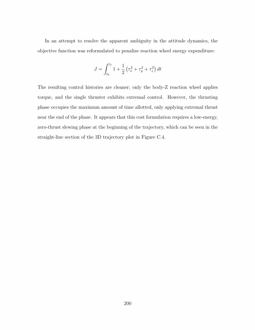
In an attempt to resolve the apparent ambiguity in the attitude dynamics, the

objective function was reformulated to penalize reaction wheel energy expenditure:

J =

∫ tf

t0

1 +1

2

(τ 2x + τ 2y + τ 2z

)dt

The resulting control histories are cleaner; only the body-Z reaction wheel applies

torque, and the single thruster exhibits extremal control. However, the thrusting

phase occupies the maximum amount of time allotted, only applying extremal thrust

near the end of the phase. It appears that this cost formulation requires a low-energy,

zero-thrust slewing phase at the beginning of the trajectory, which can be seen in the

straight-line section of the 3D trajectory plot in Figure C.4.

200

0 50 100 150

Time (s)

-1

-0.5

0

0.5

1

Quat

ernio

n M

agnitude

Quaternion Histories

q1q2q3q4Phase

0 50 100 150

Time (s)

-0.03

-0.02

-0.01

0

Rot

atio

n R

ates

(ra

d/s

)

Rotation Rate Histories

wxwywzPhase

0 50 100 150

Time (s)

0

0.1

0.2

0.3

0.4

0.5

Con

trol

Thru

st (

N)

Thruster Control History

Max/Min ThrustThrustPhase

0 50 100 150

Time (s)

-0.01

-0.005

0

0.005

0.01

Con

trol

Tor

que

(N-m

)

Control Torque History

TxTyTzPhase

Figure C.4: Attitude-coupled period-matching trajectory for chaser with one +Xthruster, objective function J =

∫ tft0

1 + 12

(τ 2x + τ 2y + τ 2z

)dt, and initial condition

x0 = [100 110 250 0.1 0.1 0.1]T

If the thruster bounds are modified to allow bidirectional thrust (simulating two

opposing thrusters along the body X axis), the result is slightly different. Instead

of an initial slewing phase, the thruster is always saturated, but switches direction

201

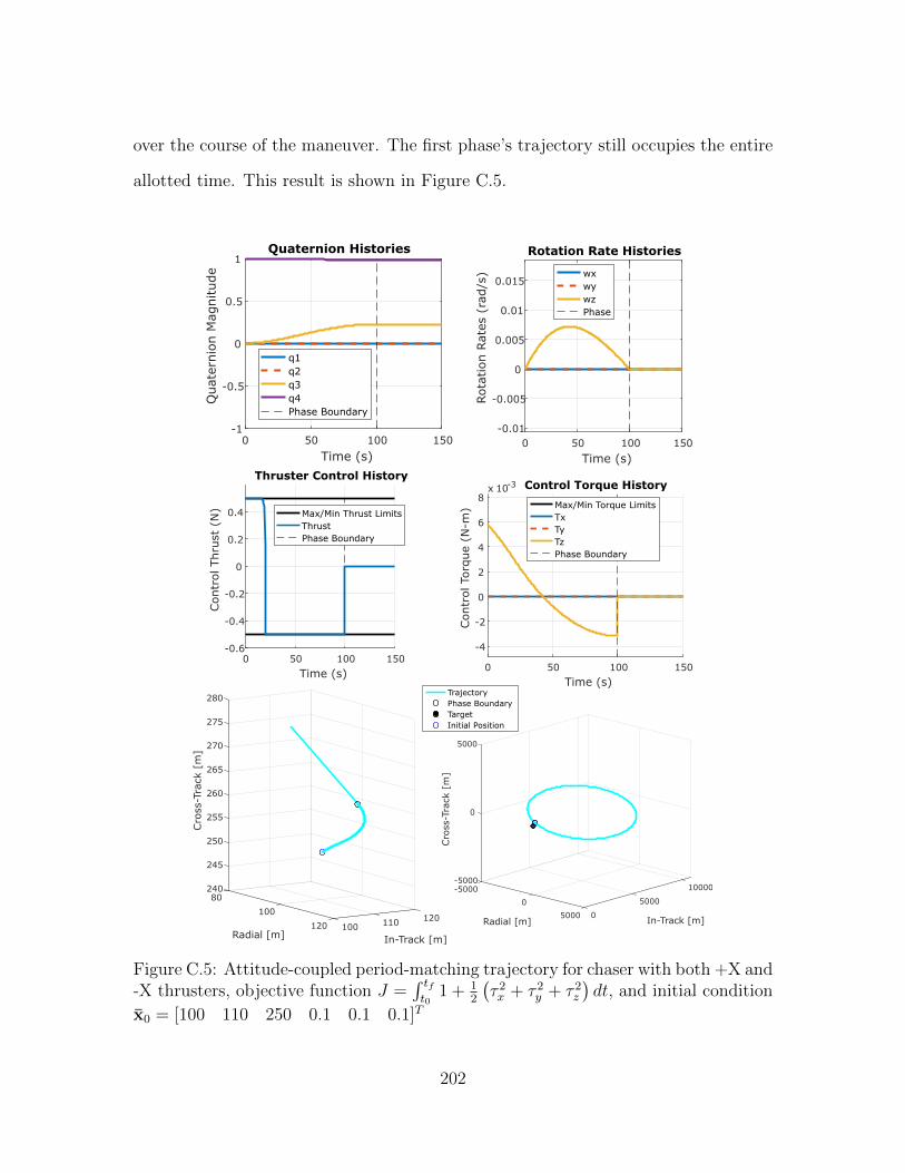
over the course of the maneuver. The first phase’s trajectory still occupies the entire

allotted time. This result is shown in Figure C.5.

0 50 100 150

Time (s)

-1

-0.5

0

0.5

1

Quat

ernio

n M

agnitude

Quaternion Histories

q1q2q3q4Phase Boundary

0 50 100 150

Time (s)

-0.01

-0.005

0

0.005

0.01

0.015

Rot

atio

n R

ates

(ra

d/s

)

Rotation Rate Histories

wxwywzPhase

0 50 100 150

Time (s)

-0.6

-0.4

-0.2

0

0.2

0.4

Con

trol

Thru

st (

N)

Thruster Control History

Max/Min Thrust LimitsThrustPhase Boundary

0 50 100 150

Time (s)

-4

-2

0

2

4

6

8

Con

trol

Tor

que

(N-m

)

x 10-3 Control Torque History

Max/Min Torque LimitsTxTyTzPhase Boundary

TrajectoryPhase BoundaryTargetInitial Position

240

245

250

255

260

80

265

270

Cro

ss-T

rack

[m

]

275

280

Radial [m]

100120

In-Track [m]

110120 100

-500010000-5000

0

Cro

ss-T

rack

[m

]

5000

In-Track [m]Radial [m]

50000

05000

Figure C.5: Attitude-coupled period-matching trajectory for chaser with both +X and-X thrusters, objective function J =

∫ tft0

1 + 12

(τ 2x + τ 2y + τ 2z

)dt, and initial condition

x0 = [100 110 250 0.1 0.1 0.1]T

202

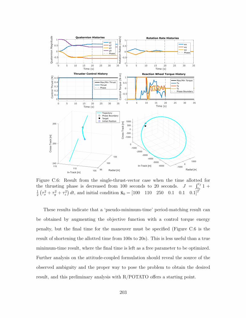
0 5 10 15 20 25 30 35

Time (s)

-1

-0.5

0

0.5

1

Quat

ernio

n M

agnitude Quaternion Histories

q1q2q3q4Phase

0 5 10 15 20 25 30 35

Time (s)

-1

-0.5

0

0.5

1

Rot

atio

n R

ates

(ra

d/s

)

Rotation Rate Histories

wxwywzPhase

0 5 10 15 20 25 30 35

Time (s)

0

0.1

0.2

0.3

0.4

0.5

Con

trol

Thru

st (

N)

Thruster Control History

Max/Min ThrustThrustPhase

0 5 10 15 20 25 30 35

Time (s)

-1

-0.5

0

0.5

1

Con

trol

Tor

que

(N-m

) Reaction Wheel Torque History

Max/Min TorqueTxTyTzPhase Boundary

TrajectoryPhase BoundaryTargetInitial Position

Figure C.6: Result from the single-thrust-vector case when the time allotted forthe thrusting phase is decreased from 100 seconds to 20 seconds. J =

∫ tft0

1 +12

(τ 2x + τ 2y + τ 2z

)dt, and initial condition x0 = [100 110 250 0.1 0.1 0.1]T

These results indicate that a ‘pseudo-minimum-time’ period-matching result can

be obtained by augmenting the objective function with a control torque energy

penalty, but the final time for the maneuver must be specified (Figure C.6 is the

result of shortening the allotted time from 100s to 20s). This is less useful than a true

minimum-time result, where the final time is left as a free parameter to be optimized.

Further analysis on the attitude-coupled formulation should reveal the source of the

observed ambiguity and the proper way to pose the problem to obtain the desired

result, and this preliminary analysis with R/POTATO offers a starting point.

203

204

Appendix D

List of R/POTATOUser-Specifiable Parameters

This appendix provides a table of flags and parameters that were designed to beuser-modifiable in the Instantiation Shell of R/POTATO. The tool can be downloadedat the following URL: https://github.com/zfunke7/R-POTATO.

Incl_Att_Dynamics Uses the attitude-coupled 6-DOF dynamics (3-DOF is default)

Min_Time Sets the objective function to minimize maneuver timeSched_Pol If MinTime is set, this enforces a ‘regulate, then wait’ policy to

resolve scheduling ambiguity for 3-DOF problemHybrid_Opt If MinTime is set, determine time to regulate limiting coordinate,

and optimize non-limiting coordinates for minimum energy on thattime interval (alternative to SchedPol for 3-DOF problem)

Min_Fuel Sets the objective function to minimize fuel expenditureOne_Phase Attempts to solve Min Fuel problem in one phaseThree_Phase Allocates three phases (bang-off-bang) for Min Fuel problemBang_Width Specifies max width of ‘bang’ periods for ThreePhase Min FuelDecoup_Bang Decouples bang on-times for in-plane vs. out-of-plane coordinates

Quadratic_Cost Sets the objective function to an LQR-like function of the stateand control inputs

Q_R_ratio Numeric value specifying the relative weighting of state regulationversus control energy expenditure

Min_Energy Sets the objective function to minimize control energy expenditure

Max_Time Specifies the maximum maneuver time for the first phase (MinEn-ergy and MinFuel only)

Table D.1: List of user-modifiable parameters specifying the objective function to beoptimized along the trajectory.

205

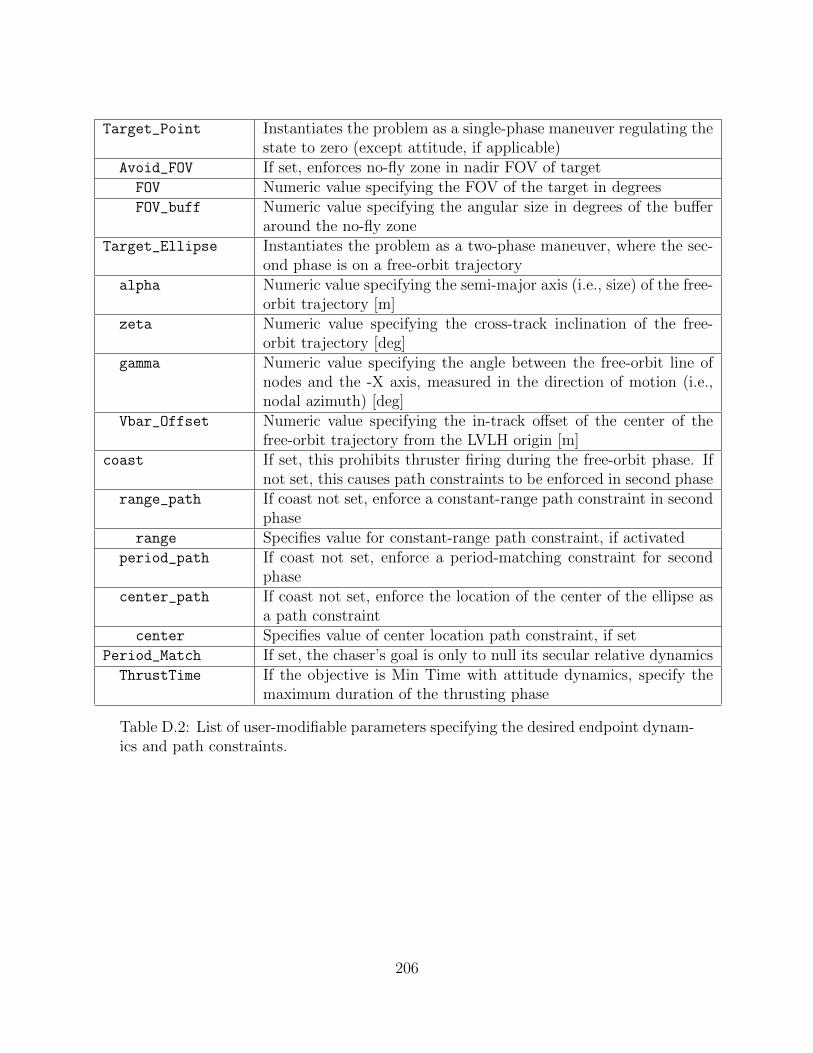
Target_Point Instantiates the problem as a single-phase maneuver regulating thestate to zero (except attitude, if applicable)

Avoid_FOV If set, enforces no-fly zone in nadir FOV of targetFOV Numeric value specifying the FOV of the target in degreesFOV_buff Numeric value specifying the angular size in degrees of the buffer

around the no-fly zoneTarget_Ellipse Instantiates the problem as a two-phase maneuver, where the sec-

ond phase is on a free-orbit trajectoryalpha Numeric value specifying the semi-major axis (i.e., size) of the free-

orbit trajectory [m]zeta Numeric value specifying the cross-track inclination of the free-

orbit trajectory [deg]gamma Numeric value specifying the angle between the free-orbit line of

nodes and the -X axis, measured in the direction of motion (i.e.,nodal azimuth) [deg]

Vbar_Offset Numeric value specifying the in-track offset of the center of thefree-orbit trajectory from the LVLH origin [m]

coast If set, this prohibits thruster firing during the free-orbit phase. Ifnot set, this causes path constraints to be enforced in second phase

range_path If coast not set, enforce a constant-range path constraint in secondphase

range Specifies value for constant-range path constraint, if activatedperiod_path If coast not set, enforce a period-matching constraint for second

phasecenter_path If coast not set, enforce the location of the center of the ellipse as

a path constraintcenter Specifies value of center location path constraint, if set

Period_Match If set, the chaser’s goal is only to null its secular relative dynamicsThrustTime If the objective is Min Time with attitude dynamics, specify the

maximum duration of the thrusting phase

Table D.2: List of user-modifiable parameters specifying the desired endpoint dynam-ics and path constraints.

206

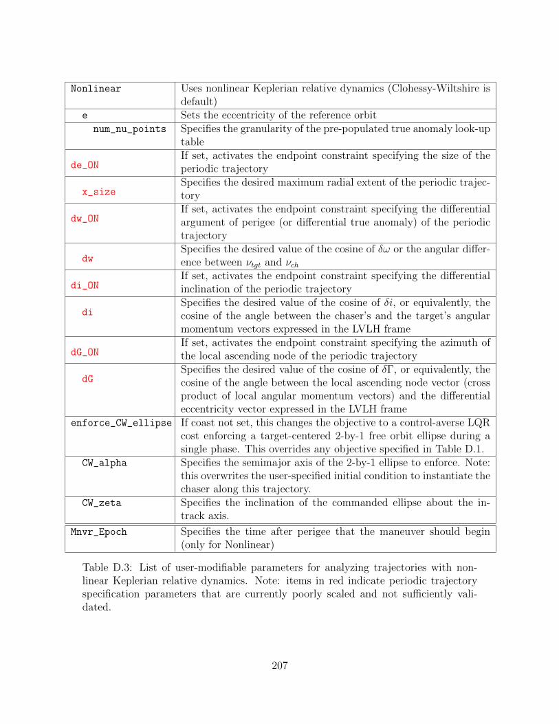
Nonlinear Uses nonlinear Keplerian relative dynamics (Clohessy-Wiltshire isdefault)

e Sets the eccentricity of the reference orbitnum_nu_points Specifies the granularity of the pre-populated true anomaly look-up

table

de_ONIf set, activates the endpoint constraint specifying the size of theperiodic trajectory

x_sizeSpecifies the desired maximum radial extent of the periodic trajec-tory

dw_ONIf set, activates the endpoint constraint specifying the differentialargument of perigee (or differential true anomaly) of the periodictrajectory

dwSpecifies the desired value of the cosine of δω or the angular differ-ence between νtgt and νch

di_ONIf set, activates the endpoint constraint specifying the differentialinclination of the periodic trajectory

diSpecifies the desired value of the cosine of δi, or equivalently, thecosine of the angle between the chaser’s and the target’s angularmomentum vectors expressed in the LVLH frame

dG_ONIf set, activates the endpoint constraint specifying the azimuth ofthe local ascending node of the periodic trajectory

dGSpecifies the desired value of the cosine of δΓ, or equivalently, thecosine of the angle between the local ascending node vector (crossproduct of local angular momentum vectors) and the differentialeccentricity vector expressed in the LVLH frame

enforce_CW_ellipse If coast not set, this changes the objective to a control-averse LQRcost enforcing a target-centered 2-by-1 free orbit ellipse during asingle phase. This overrides any objective specified in Table D.1.

CW_alpha Specifies the semimajor axis of the 2-by-1 ellipse to enforce. Note:this overwrites the user-specified initial condition to instantiate thechaser along this trajectory.

CW_zeta Specifies the inclination of the commanded ellipse about the in-track axis.

Mnvr_Epoch Specifies the time after perigee that the maneuver should begin(only for Nonlinear)

Table D.3: List of user-modifiable parameters for analyzing trajectories with non-linear Keplerian relative dynamics. Note: items in red indicate periodic trajectoryspecification parameters that are currently poorly scaled and not sufficiently vali-dated.

207

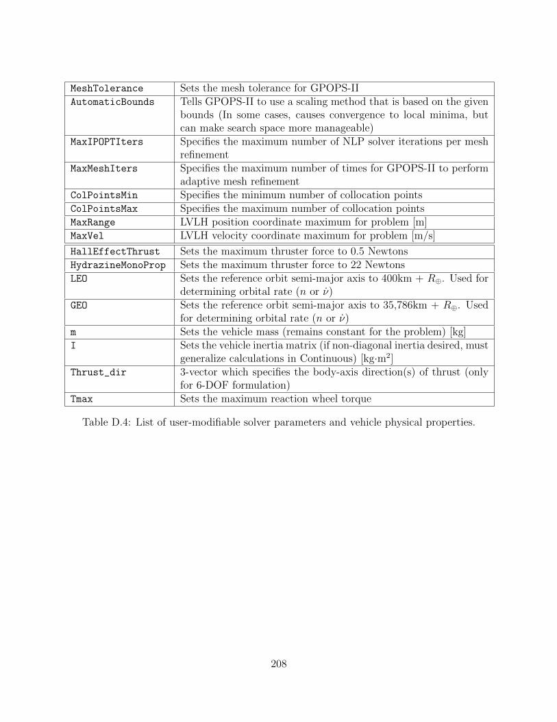
MeshTolerance Sets the mesh tolerance for GPOPS-IIAutomaticBounds Tells GPOPS-II to use a scaling method that is based on the given

bounds (In some cases, causes convergence to local minima, butcan make search space more manageable)

MaxIPOPTIters Specifies the maximum number of NLP solver iterations per meshrefinement

MaxMeshIters Specifies the maximum number of times for GPOPS-II to performadaptive mesh refinement

ColPointsMin Specifies the minimum number of collocation pointsColPointsMax Specifies the maximum number of collocation pointsMaxRange LVLH position coordinate maximum for problem [m]MaxVel LVLH velocity coordinate maximum for problem [m/s]

HallEffectThrust Sets the maximum thruster force to 0.5 NewtonsHydrazineMonoProp Sets the maximum thruster force to 22 NewtonsLEO Sets the reference orbit semi-major axis to 400km + R⊕. Used for

determining orbital rate (n or ν)GEO Sets the reference orbit semi-major axis to 35,786km + R⊕. Used

for determining orbital rate (n or ν)m Sets the vehicle mass (remains constant for the problem) [kg]I Sets the vehicle inertia matrix (if non-diagonal inertia desired, must

generalize calculations in Continuous) [kg·m2]Thrust_dir 3-vector which specifies the body-axis direction(s) of thrust (only

for 6-DOF formulation)Tmax Sets the maximum reaction wheel torque

Table D.4: List of user-modifiable solver parameters and vehicle physical properties.

208

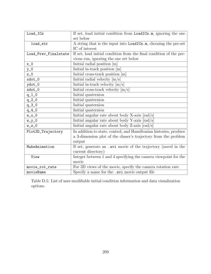
Load_ICs If set, load initial condition from LoadICs.m, ignoring the oneset below

load_str A string that is the input into LoadICs.m, choosing the pre-setIC of interest

Load_Prev_Finalstate If set, load initial condition from the final condition of the pre-vious run, ignoring the one set below

x_0 Initial radial position [m]y_0 Initial in-track position [m]z_0 Initial cross-track position [m]xdot_0 Initial radial velocity [m/s]ydot_0 Initial in-track velocity [m/s]zdot_0 Initial cross-track velocity [m/s]q_1_0 Initial quaternionq_2_0 Initial quaternionq_3_0 Initial quaternionq_4_0 Initial quaternionw_x_0 Initial angular rate about body X-axis [rad/s]w_y_0 Initial angular rate about body Y-axis [rad/s]w_z_0 Initial angular rate about body Z-axis [rad/s]

Plot3D_Trajectory In addition to state, control, and Hamiltonian histories, producea 3-dimension plot of the chaser’s trajectory from the problemoutput

MakeAnimation If set, generate an .avi movie of the trajectory (saved in thecurrent directory)

View Integer between 1 and 4 specifying the camera viewpoint for themovie

movie_rot_rate For 3D views of the movie, specify the camera rotation ratemovieName Specify a name for the .avi movie output file

Table D.5: List of user-modifiable initial condition information and data visualizationoptions.

209

210

Bibliography

[1] K. T. Alfriend, S. R. Vadali, P. Gurfil, J. How, and L. Breger. Spacecraft For-mation Flying: Dynamics, Control, and Navigation. Butterworth-Heinemann,November 2009.

[2] B. Barbee, R. Carpenter, S. Heatwole, F. L. Markley, M. Moreau, B. J. Naasz,and J. Van Eepoel. Guidance and Navigation for Rendezvous and Proximity Op-erations with a Non-Cooperative Spacecraft at Geosynchronous Orbit. Journalof Astronautical Sciences, 58(3), July 2011.

[3] R. R. Bate, D. D. Mueller, and J. E. White. Fundametals of Astrodynamics.Dover Publications, Inc., New York, 1971.

[4] R. Bevilacqua. Optimization Techniques for Satellites Proximity Maneuvers.PhD thesis, Sapienza University of Rome, 2006.

[5] A. D. Biria and R. P. Russell. Periodic Orbits in the Elliptical Relative Mo-tion Problem with Space Surveillance Applications. In AAS/AIAA SpaceflightMechanics Meeting, volume 152, January 2014.

[6] G. Boyarko, O. Yakimenko, and M. Romano. Optimal Rendezvous Trajectoriesof a Controlled Spacecraft and a Tumbling Object. Journal of Guidance, Control,and Dynamics, 34(4), August 2011.

[7] G. A. Boyarko. Spacecraft Guidance Strategies for Proximity Maneuvering andClose Approach With a Tumbling Target. PhD thesis, Naval Postgraduate School,March 2010.

[8] A. E. Bryson and Y.-C. Ho. Applied Optimal Control. Hemisphere PublishingCorporation, revised printing edition, 1975.

[9] NORAD Two-Line Element Sets: Geostationary Communications Satellites,March 2017. https://celestrak.com/NORAD/elements/geo.txt.

[10] W. Clohessy and R. Wiltshire. Terminal Guidance System for Satellite Ren-dezvous. Journal of the Aerospace Sciences, 27(5):653–658, 674, 1960.

211

[11] R. Epenoy. Fuel optimization for continuous-thrust orbital rendezvous with col-lision avoidance constraint. Journal of Guidance, Control, and Dynamics, 34(2),March 2011.

[12] W. Fehse. Automated Rendezvous and Docking of Spacecraft. Cambridge Uni-versity Press, 2003.

[13] Z. Funke. Introduction to Quaternions. Technical report, MIT Space SystemsLab, 2016.

[14] G. Gaias, S. D’Amico, and J.-S. Ardaens. Angles-only navigation to a nonco-operative satellite using relative orbital elements. Journal of Guidance, Control,and Dynamics, 37(2), March 2014.

[15] K. Großekatthoffer and Z. Yoon. Introduction into quaternions for spacecraftattitude representation. Technical University of Berlin, 2012.

[16] G. Gugliotta. Nominee Backs a Review of NASA’s Hubble Decision. The Wash-ington Post, April 2005.

[17] P. Gurfil. Relative Motion Between Elliptic Orbits: Generalized BoundednessConditions and Optimal Formationkeeping. Journal of Guidance, Control, andDynamics, 28(4), July 2005.

[18] S. R. Hall. 16.323 Lecture 8: GPOPS-II Optimization Software. MassachusettsInstitute of Technology, March 2016.

[19] J. P. How and M. Tillerson. Analysis of the Impact of Sensor Noise on FormationFlying Control. In Proceedings of The American Control Conference, June 2001.

[20] G. Inalhan, M. Tillerson, and J. P. How. Relative Dynamics and Control ofSpacecraft Formations in Eccentric Orbits. Journal of Guidance, Control, andDynamics, 25(1), January 2002.

[21] D. Izzo and M. Sabatini. Magic (Special) Inclinations for Formation Flying.Technical report, 2008.

[22] C. M. Jewison. Guidance and Control for Multi-stage Rendezvous and DockingOperations in the Presence of Uncertainties. PhD thesis, Massachusetts Instituteof Technology, June 2017.

[23] M. H. Kaplan. Modern Spacecraft Dynamics and Control. New York, John Wileyand Sons, Inc., 1976. 427 p., 1976.

[24] C. D. Karlgaard. Second-Order Relative Motion Equations. Master’s thesis,Virginia Polytechnic Institute and State University, July 2001.

212