Lolina Alvarez Alonso - cms.dm.uba.arcms.dm.uba.ar/.../Distribution-Theory-Lolina.pdf · solutions of partial differential equations and further incorporated the methods of functional

DISTRIBUTION THEORY AND FOURIER TRANSFORM

(A USER'S MANUAL)

Lolina Alvarez Alonso

Department of Mathematics

New Mexico State University

Las Cruces, NM 88003-8001

USA

E-mail address: [email protected]

ISSN N° 0326-5641

Buenos Aires, Argentina

Prohibida su reproducción total o parcial.

IMPRESO EN ARGENTINA

Se terminó de imprimir en octubre de 2000 en los Talleres Gráficos RED OLIMPICA Santa Fe 3312 9°, Buenos Aires, Argentina

Introduction

The theory of distributions is considered one of the great achievements of mathematical analysis in the twentieth century. This theory fits in many ways within the framework of mathematical analysis and mathematical physics, among other subjects. Indeed, his development provided a rigorous setting in which formal objects such as the Dirac function were fully justified. It augmented the bank of initial data and solutions of partial differential equations and further incorporated the methods of functional analysis into the study of differential operators. It rounded up the theory of Fourier transform, bringing in another great development of the twentieth century, namely the Lebesgue integral. With the theory of distributions a whole array of spaces appeared that became the foremost examples in the theory of topological vector spaces. The article by John Synowiec [5] provides a good account of sorne of these achievements. It mentions also more i;ecent uses in microlocal analysis and wavelets. For specific applications of distribution theory to the theory of partial differential equations we refer to the article by Frarn;ois Treves [ 6].

Although there are quite a few hints at the theory of distributions prior to the work of Laurent Schwartz, it is his work that definitely put the theory in its present form, and made the essential connections with the Fourier transform and the theory of partial differential equations. This blend of theories is one of the reasons why the theory of distributions has become part of mainstream mathematics. To be sure, this has not been always the case. Lars Hiirmander relates in [1] how his mentor reproached him for using distributions in his doctoral dissertation. John Synowiec reproduces in [5] the following conversation with severa! of his professors during his years as graduate student "Distribution? You mean probability distribution.- No, a Schwartz distribution.-Oh .. .if you are interested in that sort of thing you'll have to talk to somebody else. I don't have much use for them in my work."

1

2 Distribution theory and Fourier Transform

These reticencies are in the past now. As an evidence of the position that the theory of distributions enjoys at present, we can recall the words of Jeffrey Rauch in [4], " ... Distribution Theory has become so ubiquitous in analysis and geometry that one of the good things that a course in Partial Differential Equations <loes is to familiarize students with this subject."

Let me repeat that as it is the case with most theories, the theory of distributions <lid not spring full flesh from Schwartz's forehead. In his classical book, Schwartz himself provides a thorough account of many prior insights and open problems that inspired his work. Another good source is the article by John Horváth [2].

To understand how and why a piece of mathematics has become what it is now, it is very useful to learn about its historical development. It is surprising and even amusing to see how rooted in common sense and human needs are the origins of practically any piece of mathematics, regardless of the leve! of abstraction that it may have today. The theory of distributions is no exception. An account of its very intere~ting historical development can be found in the book by Jesper Lützen [3]. This book also exemplifies many applications where the need arose for a generalized notion of function.

We must mention that Laurent Schwartz's work is not the only attempt to extend the concept of function, although it is probably fair to say that Schwartz's approach has proved to be the most successful and most widely used.

The article by Jeffrey Rauch [3] ends with an extensive bibliography on the theory of distributions, including presentations of the theory a la Schwartz as well as presentations following other approaches.

It is clear then that anyone wanting to become familiar with the theory of distributions can choose from a great variety of possibilities.

I hope that still these notes serve the purpose that originated them in the first place.

Namely, to provide an efficient mathematical presentation of the theory of distributions a la Schwartz. The emphasis is on "getting the hands dirty" with sorne of the calculations that are the bread and butter of a harmonic analyst or PDE practitioner. Except for a few remarks, we do not dwell on the topoloiical structures that make things the way they are in this theory. To put it bluntly, in our presentation we choose whenever possible to do a calculation over citing a theorem. To be sure, this is not always possible, showing that the theory of topological vector spaces have a sure footing in the

Introduction 3

foundation of distribution theory. Probably the best feature of these notes is the presentation of the Fourier transform, both the classical V theory and the theory in the sense of distributions. Another good feature is the list of problems found at the end of each chapter. It has been said that mathematics is not a spectator's sport. These problems are aimed at getting you to play the game. Do not overlook them.

Shortly after these notes were written in the mid 70's, Professor Calderón read them over and expressed to me his satisfaction. This is the best assurance I can offer to a potential reader. Professor Calderón was a master in tailoring the tools he used to the scope of the results he wanted to obtain.

It is with great admiration that I dedícate this reprint to his memory.

I thank my friends of many years at the PEMA for this wonderful opportunity to renew my relationship with them and with the mathematicians on the make in Santa Fe and elsewhere.

I have tried hard, probably unsuccessfully, to weed out mistakes and misprints. I welcome any comments that the potential readers of these notes may want to send me.

Las Cruces, July 2000


Works Cited in the Introduction

[1] Hormander, Lars, "On local integrability of fundamental solutions", Ark. Mat. 37 (1999) 121-140.

[2] Horváth, John, "An introduction to distributions", Amer. Math. Monthly 77 (1970) 227-240.

[3] Lützen, Jesper, The prehistory ofthe theory of distributions, Springer (1983).

[4] Rauch, Jeffrey, "Book review", Bulletin Amer. Math. Soc. 37 (2000) 363-367.

[5] Synowiec, John, "Book review", Amer. Math. Monthly 103 (1996) 435-440.

[6] 'lleves, Frarn;ois, "Applications of distributions to PDE theory", Amer. Math. Monthly 77 (1970) 241-248.

Introduction 5

I first put together these notes in 1976 to serve asan introduction to the course that Prof. Alberto P. Calderón was going to teach on Partial Differential Equations, at the School of Sciences of the University of Buenos Aires.

Besides translating them, I have done very little on the way of revision. Particularly, I have kept the same set of references, only adding a few.

None of the concepts and very little of the presentation are mine. I borrowed from many sources and I tried to give fair credit whenever possible. However, I failed to do so in the original version with the presentation of the Fourier transform. I vaguely remember using sorne borrowed notes, but beyond that, I do not recall.

The intention of these notes, as hinted by the title, is to be used as a nontechnical introduction to the subject. For those seeking a deeper understanding ofthe theory, sorne ofthe references, mainly [1] and [2], contain a complete presentation of the matter. The original reference [1] has long ago been translated into English.

Las Cruces, July 1992

Contents

Introduction 1

Chapter l. The spaces 1J and 1)' 9

Chapter 2. The spaces S S' E E' vCmJ and 7JCmJ1

' ' ' ' 23

Chapter 3. The derivative of a distribution 35

Chapter 4. Tensor product, convolution product and multiplicative product of distributions 43

Chapter 5. The L1 and L2 theories of the Fourier transform (Preliminaries) 57

Chapter 6. The Fourier transform in the spaces S and S' 65

Chapter 7. The L1 and L 2 theories of the Fourier transform ( Conclusion) 73

Chapter 8. The action of Fourier transform on convolution products and multiplicative products. 77

Chapter 9. The Hausdorff - Young theorem 81

Bibliography 89

7

8 CONTENTS

Notation

We will denote (jj the space of complex numbers.

Given x E IRn, with lxl we will indicate the euclidean norm of x,

( 2 2)1/2 X1 + ... +xn .

However, given a= (a1,··· ,an) E INn, with lal we will denote a1 + · · · + °'n· The distintion between lxl and lal should be clear in the context.

We will also denote a!= a1! a2! · · · an!

Now, given a, f3 E IN", a;::: f3 will mean that O<j ;::: f3j , V j=l, ... ,n .

Given a, f3 E IN", if a ;::: /3, the symbol ( ~ ) will denote the product

($:)···($:)· Given X E mn' a E INn' we will denote x"' = X~1

••• X~".

Given x, ( E IR" , x.( is the dot product, a scaler product x1( 1 + · · · + Xn(n·

al"'I Given a E INn , D"' will denote

0 "''

0 .

X1 ... x~n

When it is important to indicate the order in which the derivatives are

taken, we will use the notation D;', ... rk or Dr,···rk to mean 0

ak 0

. Xr1 • • • Xrk

CHAPTER 1

The spaces V and V'

Definition 1.1: Let cp: íl -+ a:, íl e mn open. The support of cp, denoted supp ( cp), is the closure in íl of the set { x E íl / cp( x) i= O}.

A continuous function with continuous derivatives of all orders, will be called infinitely smooth .

Definition 1.2: Let

V = { cp : mn -+ a: 1 cp is infinitely smooth and supp ( cp) is compact} .

We will consider on V the following notion of convergence: The sequence {cpj} converges to <pin V if supp(cpj), supp(cp) are

contained in a fixed compact set and for each a E INn, D"cpj-+ D°'cp uniformly in mn.

Example 1.1: The function

p(x) = { 1

e - 1-1·1" lxl < 1 O lxl 2: 1

belongs to the class 'D and supp(p) = {x E mnj lxl S 1}. The function p shows that the class 'D <loes not reduce to zero;

moreover, we will use this function frequently and for reasons that will be clear la ter, we will call it a regularizing function.

Definition 1.3: A linear map T : 'D -+ a: is called a distribution if it is continuous in the following sense:

whenever 'Pj-+ o in v.

The value T ( <p) is usually denoted (T, <p ); thus, we can write the continuity condition as

(T, 'Pi) -+O whenever <pj-+ O in V.

9


The functions in the space V are called testing functions. We will use again this name in §2 applied to new function spaces.

Remark 1.1: When talking about the continuity of a map defined between two spaces, the usual approach is first to define topological structures. This is not what we have done in Definition 1.1, at least explicitly. This situation deserves some comments. Given K e llr compact, let

V (K) = {rp E V/supp (rp) e K}.

We can define on V (K) a structure of topological vector space by means of the family of seminorms

Na (rp) = supxE.IR" IDª<p (x)j,

It can be proved that the notion of convergence given in Definition 1.2 corresponds to this topological structure. Moreover, the topology in V(K) can be obtained from a metric compatible with the vector structure. Thus, the space V(K) is a metric space, which is also complete. In view of these properties, we can rewrite Definition 1.3 in the following way:

A map T : V --+ <V is a distribution if it is linear and its restriction to each space V(K) is continuous.

The explanation above tries to clarify Definition l. 3 without going into the heart of the matter. Indeed, the space V has a topological structure induced in some way by the spaces V(K). This topological structure is such that continuity can be described in terms of sequences. However, the existence of the topology allows us to think of the complex vector space of distributions as the topological dual, 1J', of V (For a detailed presentation of these topological matters, see [l], [2]).

In dealing with continuity on V or on other function spaces to be introduced later, we will always work with sequences.

Definition 1.4: A sequence {Tj} e V' converges to T in V' if for each <p E D,

(Tj, rp) --+ (T, rp).

This type of convergence, defined without any reference to the topology of the space D, is called weak convergence. However, it can

1. The spaces 'D and V' 11

be proved that this is the notion of convergence associated to the "strong topology" in JJ', (cf. [1], [2]).

Given an operator h : JJ' -+ JJ', we will say that h is continuous if it preserves weak convergence. In other words, if (h (T¡), cp) -+ (h (t), cp) for each <p E JJ, whenever (Tj, cp)-+ (T, cp) for each <p E JJ.

Examples 1.2:

i) Given 1 :S p :S oo, !et

Lfoc = {f: mn-+ <t/ f.xK E LP for each K e mn compact}

where XK denotes the characteristic function of K. We consider in Lf

0c the topology defined by the family of seminorms

Since it suffices to consider a countable compact covering of mn, we can deduce that Lf

0c is a complete metric space where the convergence

is described as fj -+ f in Lfoc if fj·XK -+ f.xK, for each K e mn compact.

We can say that Lfoc is a Fréchet space, as well as 1J (K), (cf [2]).

Given f E Lloc> we can define a distribution, denoted Ti> or some-times f_, as -

(T¡,cp) = j f(x) cp(x) dx, <p E JJ.

The map

f-+ T¡

is one-to-one. This is a very important result, which will be proved la ter.

We will often say that a distribution T is a function, meaning that :l f E Lloc such that T coincides with T¡. That is to say, (T, cp) = J f(x) cp(x) dx , 'ef <p E JJ.

ii) Given a E IRn, m E IN, we define the operator

(T!,cp) = (a~1) m cp(a)' <p E JJ.


It is not difficult to see that T;;,, is a distribution. When m = O, T0 is called the Dirac distribution or Dirac measure and it is usually denoted Óa.

The Dirac measure is the simplest example of a distribution that is not a function, in the sense defined above. In fact let us assume that :3 f E Lf0 c such that J f(x) <p(x) dx = <p(O), \/ <p E 'D.

Particularly, let us take

j = 1, 2,3, ...

where pis the function defined in Example 1.1. We have

j f(x) p(jx) dx=p(O), j = 1,2,3, ...

Taking the limit as j --+ oo we obtain p (O) =O, which contradicts the definition of the function p.

To prove that Óa is not a function for any a E JRn, it suffices to apply the proof above to jnp (j (x - a)).

We will analyze further these examples of distributions in §2. Particularly, it will be clear then the name measure, given to the Dirac distribution.

Definition 1.5: Given f, g : IRn -t <C we define formally the product of convolution, denoted f * g, as

j f(x-y) g(y) dy.

It is clear that not for any pair of functions f, g the product of convolution will be defined. However, we have the following result:

Theorem 1.1: (Young) (cf. [3], volume 2)

Given f E L1 , g E Il' , 1 :::; p :::; oo , the product of convolution

f * g belongs to Il' . Moreover, we have the inequality, usually called Young's inequality,

Remark 1.2: The result above shows that the product of convolution defines in L1 an structure of commutative Banach algebra, (cf. [4]). However, it can be proved that the product of convolution does not

1. The spaces 'D and 1J' 13

have a unit in L1 . In other words, Jjf E L1 such that f * g = g, V g E L1, (cf. Problem 1.3).

The product of convolution will be a very useful too! in severa! important results.

Theorem 1.2: Given K e mn compact and given E > O, 3 'P E 'D such that

os 'P(x) s 1 , V X E mn

lfJ(X) = 1 , V X E K

supp ('P) e € - neighborhood (K) = {x E mn /d (x, K) <E}.

Proof: Given the function p defined in Exarnple 1.1, we consider for each j = 1, 2, 3, ...

Pj(x)= j: p(jx), where e= J p(x) dx.

It is not difficult to show that Pj E 'D,

supp (pj) = {x E fil"/ lxl S 1/j} j Pj (x) dx =l.

Let X (x) be the characteristic function ofthe set K, = ~-neighborhood(K). We set

l{Jj (x) =(X*Pj)(x)= J pj(x-y) dy= K,

= j; J x(x-y) p(jy) dy. IYl9/j

We claim that 3 j0 E IN such that 'Pjo satisfies all the properties we are looking for. Indeed, 'P (x) is well defined for any x E mn. Moreover,

OS l{Jj (x) S j pj(x-y)dy =l.

Since it is valid to differentiate under the integral sign, l{Jj is infinitely smooth. Now, given x E K, y E mn, we have

d (x - y, K) S d (x - y, x) = IYI. Thus, 3 jo E IN such that x -y E K, if x E K and jyj S 1/jo.


Then given x E K

</)j0 (x) = J X (x - y) Pjo (y) dy = J Pj0 (y) dy =l.

[y[:<;l/jo

Concerning the support of 'Pjo, since given Z¡, Z2 E mn we have

Id (z1, K) - d (z2, K)I '.S: lz1 - z2I,

if x tf. 23' - neighborhood (K), is

2E E E d(x-y,K) 2: d(x,K)- IYI > 3-3 = 3·

Thus, X (x -y)= O when x r/:. ~' -neighborhood (K), IYI '.S: l/jo. Or 'Pio (x) =O. This shows that supp(<p10 ) C E-neighborhood (K).

This completes the proof of Theorem 1.2. #

Remarks 1.3: i) Theorem 1.2 remains true with essentially the same proof when instead of working in IRn, we work in an open subset.

ii) The proof of Theorem 1.2 shows the effect of taking the convolution with the function Pi: It smooths the discontinuous function x, to obtain an infinitely smooth function, which is "almost" a characteristic. This effect explains why we called p a regularizing function. We will apply the same process to distributions in §4.

Theorem 1.3: 'D is dense in V, 1 '.S: p < oo.

Proof: It suffices to approximate functions with compact support, since it is known that these functions form a dense subset of V.

Thus, given f E IJ' with compact support, we consider

where Pi is the function defined in the proof of Theorem 1.2. We can show as in Theorem 1.2 that Íi E 'D. It remains to prove that ÍJ-+ f in V.

Let us first assume that f is a continuous function. Since it has compact support, it is uniformly continuous. Thus,

lf (x - y) - f (x)I <E if IYI < l/j,

l. The spaces D and 'D' 15

for j 2 jo (E), independently of X E mn. Then,

lh (x) - 1 (x)I S j 11 (x - y) - 1 (x)I Pí (y) dy <E if j 2 jo.

This shows that {1í} converges to 1 uniformly on IRn. But from the definition of fj it is not difficult to see that the supports of ali the functions 1í are contained in a fixed neighborhood of supp(f). Thus, since 1í and 1 vanish outside a fixed compact set, uniform convergence implies convergence in lJ'.

Now, given any function 1 in lJ' with compact support and given E > O, 3 a continuous function g with compact support such that 111 - gllLP < E •

Then, if we write gj = g * pj, we have

llh - 111LP s 111j - gjllLP + llgj - gllLP + llg 111LP · Since 1í - gj = (f - g) * pj, we can use Young's inequality to get

111J - gjllLP S 111 - gllLP llPJllv = 111 gllLP · Thus,

111J - 111LP s 2111 - gllLP + llg - gjllLP · This shows the convergence of 1í to 1 in lJ' . Then, the proof of

Theorem 1.3 is completed. #

Remarks 1.4: i) As a consequence of Theorem 1.3, we can prove that given 1 E LP, the sequence 1í = 1 * Pí will converge to 1 in V.

In fact, Jet 1R be the truncation of 1,

{ 1(x) lxlSR

1R (x) = O otherwise R = l, 2' ···

111 1í11LP s 111 - 1RllLP + 111R - 1R * PJllLP

+ 111R * Pí 1JllLP s 2111 1RllLP + 111R - 1R * PíllLP. Observe that although fj will be an infinitely smooth function, it

will not have in general compact support. The fact that 1 * PJ --+ 1 in lJ' justifies the name approximate iden

tity, given to the function PJ, (cf. Problem 1.3).

ii) With the notation of i), given E > O 3 j R E IN such that

111R * Pí 1 llLP < E.


In fact,

Theorem 1.4: The map

Lfoc-+ 1)'

f-+ T¡

is injective.

Proof: We have to prove that

j f (x) <p(x) dx =O V <p E 1J implies f =O a.e.

Given <p E 7J, Jet us consider the function

(f 'P) * Pj (X) = J f (y) 'P (y) pj (X - y) dy.

If we fue X E JRn, the function

y-+ <p(y) Pj (x-y)

belongs to 1J. Thus, (f <p) * pj (x) =O . According to Remark 1.4 i), the sequence {(f <p) * PJ} converges

tof<pinL1.

Thus, f<p =O a.e. Since <pis any function in 1J, we conclude that f =O a.e.

This completes the proof of Theorem 1.4. #

Definition l. 6: A distribution T E 1J' vanishes in the open set n e IRn if (T, <p) = O, V 'P E 1J with supp( <p) e n. It is denoted Tln = O.

For instance, the Dirac distribution 80 vanishes in any open set that does not include a.

Given distributions T1, T2 E 7J', we will say that they coincide on the open set n if (T1 - T2) In =O.

The concept of distribution can also be defined in an open set ne mn.

In fact, if 1J (il) denotes the subspace of al! functions <p E 1J with supp( <p) e n, a distribution on 1J ( n) will be a linear operator T : 1J (il) -+ <V such that the restriction of T to each space 1J (il; K) is

1. The spaces D and D' 17

continuous. With 1J (!1; K) we denote the space of functions in 1J (!1) with support contained in the fixed compact set K e !1.

We will denote 1J' ( !1) the space of such linear, continuous operators T.

Theorem 1.4 remains valid with an almost identical proof in 1)' ( !1). The function ~ 1. V', (cf. Problem 1.2 a) ), but ~ E 1)' (!1), for

any open set !1 e IR such that O 1. !l.

We have seen briefly what it means to restrict a distribution to an open set. We now want to consider the problem of extending a distribution. More concretely, we have distributions T1 , T2 with Ti E 1>' (!li), i = 1, 2 and with the property that T1 and T2 coincide in !11 n!12. Is there a distribution TE 1J' (!11 U !12) such that Tlo, = T;?

The answer to this question is yes even in a more general form. To show this, we first need to state the following result:

Theorem 1.5, (cf. [1]' volume 1): Given !1 e mn open, !et {!li};EJ be an open covering of !1 . Then 3 functions ai : !1 -+ <V infinitely smooth, such that

ai(x) 2: O 'V x E !1,

supp(ai) e !li.

For each compact set K e !1 at most a finite number of functions a; are not identically zero in K.

For each x E !1,

Definition l. 7: A family of functions satisfying the conditions of Theorem 1.5 is called a partition of unity associated to the covering { !li}.

The following simple example in the real line,

18 Distributíon theory and Fourier Transform

l

n,

shows that if we want to have one function <Xi per open set ni, then the function <Xi will not have compact support. However, if we allow more than one function °'i per set ni, we can construct them with compact support:

11 ••• . ....

n,

In other words, the statement in Theorem 1.5 can be rephrased in the following way: Given n e mn open, !et {n};EI be an open covering of n. Then, ::¡ functions <Xj : n--+ C, j E J such that

'ef X E n, for each j E J, ::¡ i E I such that <Xj E 1J (ni),

for each compact set K e n at most a finite number of functions <Xj

are not identically zero in K, for each x E n, ¿:; °'J (x) =l. jEJ

Now we are ready to solve the extension problem we mentioned abo ve

Theorem 1.6: Let {ni};EI be a family of open subsets of mn. For each !1;, !et T; E 1J' (!1;) such that T; coincides with Tj in ninnj, whenever this intersection is not empty.

1. The spaces V and V' 19

Then, if n = LJ ni, :J! distribution T E 1>' (n) such that Tln, coiEI

incides with T;, for each i E J.

Proof: Given <p E 'D (n), we can write

where { CXj} JEJ is a partition of unity associated to the open covering {ni}iEI of n, with °'J having compact support. It is understood that only a finite number of terms in the series above is not identically zero.

Now, for each j, :Ji = i (j) E I such that aj E 'D (ni)· Then, we define the map

T ( 'P) = L ('Ii(j), CXj<p) . j

It is clear that T is a linear map. We claim that it is also continuous. In fact, if 'Pe-+ O in 'D (n), particularly, supp ('Pe) is contained in a fixed compact set K e n, V f. Then, we can write as before

'Pe = L °'J 'Pe jEJ

where the number of non identically zero terms has a finite upper bound independent of f.

If aj E 1> (ni) for sorne i = i (j) E I, we can say that °'J <pe -+ O as f-+ oo, in 1> (ni)· Thus,

('Ii(J),cxJ 'Pe)-+ O as f-+ oo

because by hypothesis 'Ii(J) E D' ( ni(j)). Then, (T, <pe) -+ O as f -+ oo. This shows that TE D' (n). Let us now prove that Tln, coincides

with Ti, for each i E J. In fact, given (niJ for any i0 E I fixed, we can write again

'P = L CXj 'P· jEJ

As we said before, given °'J' :J i = i (j) E I such that (ni)· Thus, the product CXj'P has support contained in the intersection nin niº· Since we have defined (T,<p) = ¿:.: ('IicJl'°'j'P) and we know that

jEJ

20 Distribution theory and Fourier Transforrn

T;(j) coincides with 1';0

in 1J (r!i n r!ioJ, we can write the sum above as

L (Ti0 , O<j<p) = (Ti0 , L O<j<p) = (1'; 0 , 'P) · jEJ jEJ

So, we have proved that T coincides with T; in 1J ([!,;), for each i E J.

It only remains to show that there is only one distribution T E 1J' (r!) such that Tln, = T;, for each i E I .

Indeed, let T, S be distributions in 7J' ( [!) both satisfying the property above. Then, given <p E 1J (r!), we can write as before <p =:E aj 'P·

as

Using the linearity of T we obtain (T, cp) =:E (T, O<j<p). j

Since O<j'P E 1J ( r!i(j)) and TJn,c;l = T;Ul, we can write the above

j ,

But also SJn,cn = Ti(j)· So the sum we just obtained is equal to

~ (S, °'j'P) = ( S, ~ aj<p) = (S, cp).

Thus, T=S. This completes the proof of Theorem 1.6. #

Remark 1.5: If we apply Theorem 1.6 to the case T; = O for every i E J, we obtain the following important conclusion: Given a family of open sets and given a distribution that vanishes on each set of the family, the distribution also vanishes on the union of the sets.

This remark justifies the following definition:

Definition 1.8: Given TE 7J' the support of T, denoted supp(T), is the complement of the largest open set where T vanishes. In other words,

supp(T) = IRn\ U{í! e mn¡ TJn =O}.

For example, supp(óa) ={a}. In §2 we will consider the subspace of 1J' that consists of distribu

tions with compact support.

1. The spaces D and D' 21

PROBLEMS

1.1 Show the existence of the following continuous strict inclusions

1 :S q <p'.S OO.

1.2 a) Show that the function x _, ~ does not define a distribution. b) Given E X

and that this correspondence defines a distribution. This distribution is called the principal value of l and it is deno-

1 X ted p.v. ;:·

e) For each j = 1, 2, 3, ... consider the function

{ l if lxl > l

fj ( x) = O otherwis~ Prove that Tt; _, p.v.~ as j _, oo.

1.3 Show that ,a f E L 1, such that f * g = g, V g E L 1

.

H int : Suppose that such f exists and take as g the characteristic function of cubes.

1.4 a) Given T E 'D' show that x E supp (T) ~ for each open neighborhood V of x, 3 <p E 'D (V) such that (T, <p) f O.

b) LetTE'D', <pE'Dbesuchthatsupp(T)nsupp(cp)0

0. Show that (T, <p) = O.

e) Given a continuous function J: mn _,<V, prove that supp (f) = supp (T¡) . What can be said when f E Lfoc is not continuous?

1.5 Given <p E 'D, show that

supp (cp (x +y)) C { (x, y) E JR,2n jx +y E supp (cp)}.

CHAPTER 2

The spaces S S' E E' V(m) and V(m)i ' ' ' '

We will introduce in this chapter severa! spaces of testing functions. These spaces will determine, by duality, subspaces of the space D'.

We will see later the reasons for introducing these new spaces.

Definition 2.1: Let[= {cp: IRn-+ W/cp is infinitely smooth}. Weconsider in E the following notion of convergence.

The sequence { cpj} converges to cp in E if for each a E INn, the sequence D°'cpj converges to D"'cp, uniformly on each compact subset of mn.

Definition 2.2: We say that an infinitely smooth function cp : IRn -+ <J) is rapidly decreasing at infinity with ali its derivatives if for each a, f3 E INn, :J C = C (a, f3) >O such that

sup lx°'D,Bcp(x)I :S C. xEfiln

We will denote with S the vector space of all the functions rapidly decreasing at infinity with all its derivatives.

We consider in S the following notion of convergence: The sequence { C¡:>j} converges to cp in S if for each a, f3 E INn, the

sequence x°' D.8 cpj converges to x°' D.8 cp, uniformly in IRn.

Theorem 2.1: We have the following continuous and dense inclusions:

1J '-+ S '-+ E.

Proof: It is clear that as sets, 1J is contained in S and S is contained in E.

It is clear also that the convergence in 1J is stronger than the convergence in S and that this one is stronger than the convergence in E.

It only remains then to prove that each space is dense in the next one. Let us see that 1J is dense in S.

23


Let 1/JE V be a function satisfying:

O "'5.1/l(x) "'5_ l,

1/;(x)={~ if !xi -:;_ 1 if lxl "'5. 2

Theorem 1.2 shows the existence of such a function. Set

1/;j (x) = 1f; (x/j).

Given <p ES, we claim that the sequence {<p1f;j} e V, converges to <p in S.

To prove this claim, we need to show that given a, f3 E !Nn, the sequence { x" DJ3 ['P (1/;j l)J} converges to zero, uniformly in JH:'. In fact, if f3 # O, using Leibniz rule, ( cf. Problem 2.3), we can write

x"DJ3 [<p(1/;j -1)] (x) = (1/lj -1) (x) x"DJ3<p(x)

+ '¿,0<'Y:S/3 C'Yx" DJ3-'Y'P (x) (y y'YI (D'Y1f;) (y).

If /3 = O, we only have the first term in the expression above. So, it suffices to study the case f3 # O.

Each term in the sum can be estimated as

with the constant C not depending on j. Thus, the second term converges to zero, uniformly in mn as j

goes to infinity. Let us consider the first term. Since <p is rapidly decreasing with all its derivatives, exists

lim lx" DJ3 (x)I =O. On the other hand, 1 -1/;j (x) =O if !xi -:;. j. lxl-400

Then,

sup 1 [1 -1/Jj (x)] x" D¡3j

Thus, we have proved that V is dense in S. To prove that S is dense in E it suffices to show that V is dense in E. Given <p E E, we

2. ThespacesS,S',é.,é.1 ,D(m) and vCm)t 25

claim that the same sequence { <f"IPÚ e 'D we considered in the first part, will converge to r.p in & as j --+ oo.

Indeed, given any compact subset K of IRn, 3 j 0 = j 0 (K) such that 1/Jj (x) = 1 on a neighborhood of K, V j ::'.'. j 0 .

This shows that far any a E JN7', the sequence D°' ( r.p'l/Jj) will converge unifarmly to Dªr.p on K, in a trivial way.

This completes the proof of Theorem 2.1.#

Definition 2.3: A linear operator T : S --+ <V is called a temperate distribution if it is continuous in the usual way. N amely,

whenever in S.

The vector space of ali temperate distribution will be denoted with S'. The operators in S' are indeed distributions in the sense of Definition 1.3. In fact, given TE S', since according to Theorem 2.1 there is a continuous inclusion 'D '-+ S, the restriction of T to 'D will be long to 'D'. Thus, in the sense of this restriction, S' is contained in 'D'. We will see in §3 a reason far the name temperate.

Definition 2.4: We denote with &' the space of ali the linear and continuous operators T : & --+ <V. By restriction, the operators in &' will define distributions which are temperate. However, we cango further in describing the space &'-. In fact,

Theorem 2.2: &' can be identified with the subspace of V' of ali the distributions with compact support.

Proof: Let K ={TE 'D'/ supp(T) is compact} we consider the restriction map

&' .:::_, V'

T --+ T/'D

We will show that this map is a bijection of &' onto K. In fact, given T E &', Jet T1 = T/'D. We claim that T1 E K.

Indeed, if supp(T1) is not compact, then given k = 1, 2, ... , 3 'Pk E 'D with supp(r.p) e {x E mn¡ lxl ::'.'. k} and (T1 ,r.pk) #O. We can assume (T1,cpk) =l. Since the sequence {r.pk} converges trivially to zero in&, we deduce that (T, 'Pk) = (T1, 'Pk) should converge to zero as k --+ oo. Thus, T1 E K .

26 Distribution theory and Fourier Thansform

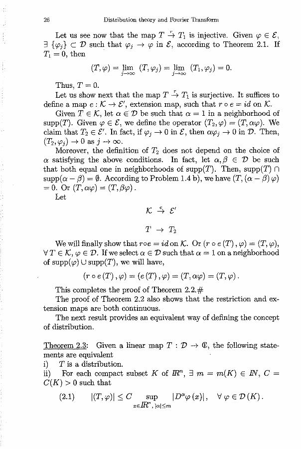
Let us see now that the map T -0 T1 is injective. Given <p E E, 3 {'Pj} e V such that <{Jj --+ <pin E, according to Theorem 2.1. If T1 =O, then

Thus, T =O. Let us show next that the map T -0 T1 is surjective. It suffices to

define a map e : K --+ E', extension map, su ch that r o e = id on K. Given T E K, !et a E V be such that a = 1 in a neighborhood of

supp(T). Given <p E E, we define the operator (T2,<p) = (T,a<p). We claim that T2 E E'. In fact, if 'Pj--+ O in E, then a<pj --+O in V. Then, (T2, '/)j) --+ o as j --+ OO.

Moreover, the definition of T2 does not depend on the choice of a satisfying the above conditions. In fact, !et a, (3 E V be such that both equal one in neighborhoods of supp(T). Then, supp(T) n supp(a - (3) = ©. According to Problem 1.4 b), we have (T, (a - (3) <p) =O. Or (T, a<p) = (T, (3<p).

Let

K -é+ E'

T --+ T2

We will finally show that roe = id on K. Or ( r o e (T) , <p) = (T, <p ), V T E K, <p E V. If we select a E V such that a = 1 on a neighborhood of supp(<p) U supp(T), we will have,

(roe(T),<p) = (e(T),<p) = (T,a<p) = (T,<p).

This completes the proof of Theorem 2. 2. # The proof of Theorem 2.2 also shows that the restriction and ex

tension maps are both continuous. The next result provides an equivalent way of defining the concept

of distribution.

Theorem 2.3: Given a linear map T : V --+ <U, the following statements are equivalent i) T is a distribution. ii) For each compact subset K of IR', 3 m = m(K) E IN, C = C(K) > O such that

(2.1) [(T, <p)[ ::; C sup [D°'O, m E IN, 3 cp E D(K) such that

l(T, cp)I > e sup ID°'cp (x)I. xEfil",lal'.':m

Particularly, we can pick C = m. Then, 3 'lj;m E D(K) such that

l(T, 'lj;m)I > m sup ID"'lj;m (x)I. xEfil",lal'.':m

L 'lj;m

et 'Pm = (T, 'lj;m) Given /3 E INn, if m ::'.:: l/31, we have

1 sup ID13cpm (x)I ::; sup IDªcpm (x)I < -.

mn mn m XE.Ln, XE.Ln, i jal$m

Thus, 'Pm -+ O in D, as m -+ oo. However, by construction, we have (T, 'Pm) = 1 V m . This shows that T cannot be a distribution.

ii)==?i) Let { cpJ} e D such that 'Pj -+ O in D. Then, particularly, cpj E D(K) for sorne compact subset K e mn. Moreover each derivative Dªcpj will converge to zero, uniformly on mn.

Thus,

l(T, 'Pj)I ::; e sup IDªcpj (x)I -+o as j-+ OO.

xEfil",lal'.':m


Definition 2.5: When the number m in condition (2.1) can be picked independent of the compact set K, we say that the distribution T has finite order ::; m. Otherwise, we will say that T has infinite order.

We will denote D1(m) the subspace of D' of all the distributions of finite order ::; m.

Roughly speaking, the number m is an upper bound for the number of derivatives of the testing function that we need, to check that the operator is continuous.

Definition 2.6: Given m E IN, !et

D(m) = {cp: mn-+ ©/cp is continuous, it has continuous derivatives of order ::; m and supp ( cp) is compact}.


In V(m) a sequence { 'PJ} will converge to <p if 3 K C IRn compact such that supp(cpJ) e K 'ef j and

Dª'PJ-+ Dªcp uniformly on IRn, for each lal :::; m.

It is clear that V e vm and that the inclusion is continuous. Using a regularizing sequence {pJ}, we can also prove that the inclusion is dense, (cf. Problem 2.8).

We will denote with V(m)i the space of ali linear and continuous ftmctionals T : v<m) -+ <C. Dueto the continuous inclusion V '-+ V(m),

the operators in V(m)i define by restriction, distributions in V 1•

However, we can say more:

Theorem 2.4: The spaces V(m)i and V 1(m) can be identified.

Proof: The proof of this result is similar to the proof of Theorem 2.2. We will show that the restriction map r : v<mJi -+ V 1 is a bijection

from V(m)! onto V 1(m). Indeed, given TE V(m)i the restriction rT = T1

belongs to V 1 because V'-+ V(m). Moreover, we claim that T1 satisfies conditibn (2.1), for this number m, independent of K. In fact, if that were not true, we could find a compact set K e mn and a sequence { 'PJ} e V (K) such that, as in the proof of Theorem 2.3,

1 = l(Ti, 'PJ)I > j sup IDª'PJ (x)I. xEIRn, jaj:Sm

From this inequality we conclude that 'PJ -+ O in v<mJ. However, (T1, 'PJ) f+ O. Thus, T1 E V 1Cm).

Let us see now that the map r is bijective: That the map is injective follows from the dense inclusion V' '-+ v<ml. Again, to prove that it is surjective it suffices to construct an extension map e : vr(m) -+ V(m)r

such that r o e. = id on vi(m).

Given TE 'D'(ml, by definition T satisfies condition (2.1) with this number m independent of K. Now, given <p E vCml, !et {'PJ} e V be a sequence such that 'PJ-+ <pin vi(m). Condition (2.1) shows that the sequence { (T, 'PJ)} is a Cauchy sequence in <C. Now, we define the operator e( T) as

(e(T), cp) = .lim (T, 'PJ). J-'>00

This definition does not depend on the sequence used to approximate <p E V(m). Indeed, if 'PJ -+ <p, and also '1/JJ -+ <p, then,

(T, 'PJ - 'ifJJ) -+ O as j -+ oo.

2. The spaces S,S',EiE'i vCm) and vC=) 1 29

Moreover, e (T) belongs to 1J(ml1• In fact, the linearity is clear, by

definition. Now if '{Jj--+ cp in 1J(m), 'h E 1>, condition (2.1) will read

l(T,cpj)I::; e sup ID"cpj (x)I xEfiln, l<>l:Sm

with C, m independent of j. Thus, taking the limitas j --+ oo, we conclude that T(e) is continuous on 1J(m). Or T(e) E 1J(ml1• Finally we will see that ro e (T) =T. In fact, if cp E 1>, we can take 'Pj = cp V j, to approximate cp. Thus,

(roe(T),cp) = (e(T),cp) = (T,cp), V cp E 1>.


Remarks 2.1: i) The proof of Theorem 2.4 shows that a linear map T: 1J(m) --+<V will belong to 1J(mJi '* given K e mn compact, :J C = C(K) > O

such that

l(T,rp)I::; e sup ID"rp(x)I, V 'PE 1J(m).

xEfil", jal:Sm

ii) We can also deduce from Theorem 2.4 that the distributions of order zero are exactly the operations that extend to linear and continuous maps from 1J(o) to <V. According to the F. Riesz representation theorem, (cf. [3], volume 1), these maps are in a bijective correspondence with the Radon measures. That is to say, given T E 1J(0 l1

, :J! Radon measure µ with complex values, such that

(T, cp) = J cpdµ

This is the way set measures are introduced in 1>', by means of identification with the distributions of order zero. Thus, in this context the word measure means both the set functions and the linear and continuous functionals on 1)(0

).

Going back to Examples 1.2, it is clear that ºª is a distribution of order zero. This is why it is called Dirac measure. The distribution 00 is associated to the real, positive and finite Radon measure,

if a E B otherwise

30 Distribution theory and Fourier 'Ifansform

where B is any Borel set in IRn. Given f E Lfoc , it is also clear that the distribution T¡ has order zero. However, the distribution associated to locally integrable functions are a special subset within the space of measures. In fact they correspond to those Radon measures that are absolutely continuous with respect to the Lebesgue measure. Since µ0 is singular with respect to the Lebesgue measure, 80 cannot have associated a locally integrable density.

Roughly speaking, the distribution 80 is the simplest example of a measure that it is not a function.

On the other hand, when m # O, the distribution T;;, defined in Examples 1.2 ii) are not measures. Indeed, r;:; has order ::::; m but it does not have order ::::; m - l.

2. ThespacesS,S1,f,f11 D(=) and v(=)' 31

PROBLEMS

2.1 i) Show that the distribution pv~ belongs to 'D1C1l. X

ii) Given p E m, p < n + 1 and given a E 'D such that a = 1 in a neighborhood of zero, show that the formula.

j lxl-p [cp (x) - a (x) cp (O)] dx, cp E 'D

IR,"

defines a distribution with order ~ l.

2.2 Show that the map

'P --+ :E 'P(j) (j) j?:O

where cp E 'D (IR,) , is a distribution with infinite order.

2.3 Given cp, 'l/; E E and a E Jl'r, show that

Dª (cp'l/;) = L ( ª) D/3cpDª-/3'l/;. f3Sa f3

[This is the Leibniz rule for the derivative of a product J .

2.4 i) Given cp E E, prove that the following statements are equivalent. a) cpES. b) For each f3 E INn and each polynomial P E ([; [x], 3 C -C ((3, P) > O such that

sup jD13 [P(x) cp(x)]j ~C. xEfiln

e) Given k E IR,, f3 E J/'r, 3 C = C (k, (3) >O such that

sup" 1(1 + lxl2)k D13cp(x)I ~C. xEJR,

ii) Using the equivalent statements given in i), obtain other ways of describing the convergence in S.

32 Distribution theory and Fourier 'fransform

iii) Show that there is a continuous inclusion S Y V', 1 :S p :S oo. Also, show that this inclusion is dense when p < oo.

2.5 i) Given r E fil, show that

[This inequality is called Peetre's lemma] .

ii) Show that the convolution product

is well defined and continuous from S x Sto S. Conclude that the convolution product defines in S an algebra structure compatible with its topology. Is there a unit?

iii) The same as ii), with respect to the multiplicative product

(rp.'lf;) (x) = rp (x) .'lf; (x).

2.6 i) Show that e-1flxl' E S and that

J e-1flxl' dx = l.

IR"

ii) Show that the function e-lxl' eiexp(lxl') is rapidly decreasing, but not its derivatives.

iii) Show that the inclusions

vese& V'::::> S' ::::> &'

are strict. Hint: Given f = elxl', ,z:J TES' such that Tlv = T¡.

iv) Show that there is a continuous inclusion V' Y S', 1 :S p :S oo. Is the same true about Lf

0c?

2. The spaces S)S',E,E', vCm) and vcm>1 33

v) A function f : JIC ---+ <V is said to be slowly increasing if 3 k E IN, C = C(k) >O such that

sup f(x) k ::;c. xEfil" (1 + lxl2

) -

Show that every measurable, slowly increasing function defines a temperate distribution.

vi) Given T E S', show that T is uniquely defined by its restriction to D.

2. 7 Show that every distribution in t:1 has finite order and that

sup { order of T /T E t:1} = oo.

2.8 Using a regularizing sequence, show that 'D is dense in 'D(m), \;/

m?: O.

2.9 Show that the space <V [x] of complex polynomials is a dense subspace of t:.

Hint: Given 'P E E, it suffices to approximate 'P with entire functions, ( cf. [5]). Consider

2.10 Change of variable in distributions:

Let !11, !12 be open subsets of mn and let </> : !11 ---+ !12 an infinitely smooth map that is proper. That is to say, for each K compact subset of !12 , .p-1 (K) is a compact subset of !11•

Then given TE 'D1 (!11), show that the operator

(Tq,, 'P) = (T, iP o 'P), 'PE 'D (!12)

defines a distribution in 'D1 (!12). What can be said about the order of Tq,, knowing that the distribution T has order ::; m?

CHAPTER 3

The derivative of a distribution

Given a distribution TE V', we want to definen distributions, called the n partial derivatives of T with respect to the variables Xi, ... , Xn

We will do this in a way that extends the usual notion of partía] derivative of a function. In other words if T = T¡ with f E 0 1

, then the distribution "jth-partial derivative of T" will be the distribution Ti:!¡ ¡ i:lx; . Let us start with this case and let us take, for simplicity in the notation, j =l. Then, given <p E 'D,

(T&¡ /i:lxp'P) = J :~ (x)cp(x)dx. IRn

If we write x = (x1, x'), x' E mn-1, and use integration by parts

in the variable x 1 , the above integral becomes,

That is to say, the integrated term is zero because the function <p vanishes outside a compact set. Thus, we can write,

(T&¡ /&x,, cp) = - (T¡, ocp /8x1).

If instead of T¡ we consider now any distribution T E 'D', we observe

V --+ <D

'P --+ - ( T, :~) is well defined and it is linear. Moreover, if 'Pk--+ O in 'D, it will also be true that ocpk/ OXj --+ O in V and then, (T, &cpk/ OXj) -+ O as k --+ oo. This shows that the map above is a distribution in V'.

35


Definition 3.1: Given T E 1Y, the distribution

'P -+ - (r, acp ) axj

is called the partial derivative of T with respect to the variable xi and it will be denoted J:, .

This process of computing partial derivatives of any given distribution can be iterated indefinitely. Thus, distributions are in this sense infinitely smooth. Moreover, since given <p E D, it is true that

az'P az'P 'ef 1 ~ j, k ~ n -

8xj8Xk 8xk8Xj'

the result of differentiating a distribution <loes not depend on the order in which the derivatives are computed.

Thus, given a E !Nn, we can write

(DªT,cp) = (-1)1ª1 (T,D°'), a E D.

In a completely analogous way we define the derivatives of distributions in S' and E'.

Example 3.1: The distribution T;;,, introduced in Examples 1.2 ii),

coincides with the distribution ( -1 )m ( 8~ 1 ) m Óa.

Theorem 3.1: If A denotes any of the spaces D', S' or E', the operator Dª is linear and continuous from A into itself. Moreover, given TE D', supp(DªT) e supp(T).

Proof: We will work in the case A= S', the other cases being the same.

If T E S', the distribution D°'T will also belong to S', because Dª'Pi-+ O in S whenever '{Jj-+ O in S.

The linearity of the operator D"' is clear. Finally it is also continuous from S' into itself. Indeed, if Tj -+ O in S', then the sequence {D"'TJ} will also converge to zero in S', because .given <p ES,

as j-+ oo.

Now, given TE D' and given <p E D with supp(cp) C 1Rn\supp (T), we have

3. The derivative of a distribution 37

because supp(D"(f)) e supp((f)). This completes the proof of Theorem 3.1.#

That a function f admits a partial derivative with respect to Xj at the point x, means that the following pointwise limit exists

l. f (xi, ... , Xj-l, Xj + hj, Xj+i, ... , Xn) - f (x) 1m .

h;->0 hj

Now, if h =(O, ... , hj, ... ,O) and Lh denotes the translation operator, (r_h f) (x) = f (x + h), we can write the limit above as

lim (r_h f) (x)- f(x) = 8f (x). h-+O hj 8xJ

It is possible to obtain a similar result for a distribution, if we extend the above notation.

In fact, the operator Lh is easily seem to be linear and continuous from D into itself. Thus, we can define the translation operator on D' as

(f) E D, TED'

which is a simple change of variables, if T = Tf, and we also obtain that ThT E D, the map T -+ ThT being also linear and continuous from D' to itself.

Thus, we can now prove the following result:

Theorem 3.2: There exists

l. T_hT-T [)T IID =-,

h-+O hJ [)xJ

meaning that for each (f) E D, there exits

l~ (r_h~J-T,(f)) = -(T, :~).

Proof: Since we have the equality

( L1i~j-T' (f)) = (T, Th~; (f))

it suffices to show that the "sequence" { 7 "'f::;"'} converges to -1!; in

D, as h-+ O.


First of all, supp ( <p(x-~,-<p(x)) will be contained in a compact

subset of IRn not dependent on h, if we assume, for instance, that o < lhl :s: l.

On the other hand, since

D~<.p (x - h) - D~<.p (x) hj

it suffices to show that <p(x-~-<p(x) converges to --i¡f (x), uniformly on J J mn, as h---+ o.

This is proved by applying twice the Mean Value Theorem,

l <p(x-1~-<p(x) + 8<.p (x)I = _ 8<.p (~) + 8<.p (x)I J 8xJ 8xJ 8xJ

- ~~ (r¡)l lx - ~I where the intermediate points ~ and r¡ belong, respectively, to the intervals with end points x, x h and x, ~·

Thus, we have showed that

1

8<.p () i.p(x-h) sup" 8x· X + h·

xElR J J

as h---+ O.


A main purpose in defining the concept of distribution, it is to be able to differentiate in sorne way, continuous functions. The definition given in this chapter can indeed be applied not only to continuous functions, but also to merely locally integrable functions. However, the following result, which we will not prove, shows that we are not too far off from our initial goal.

Theorem 3.3: (Cf. [1], volume 1): Given TE D' and given any open bounded set Q e IRn, there exists a continuous function F : Q---+ <C anda number m = m (!1) E IN such that, in the sense of distributions,

8mn T =

8 m

8 m F, in Q.

X1 .•• Xn

Remark 3.1: Theorem 3.3 shows that any distribution restricted to a bounded open set has finite order. Thus, Problem 2.2 shows that


the restriction "O bounded" cannot be eliminated.

We will now state, also without proof, another representation theorem, which explains why distributions in S' are called temperate.

Theorem 3.4: (Cf. [1], volume 2):

Given T E S', ::J a continuous, slowly increasing function F ( cf. Problem 2.6 iv)), and an n-tuple a E INn such that, in the sense of distributions, T = Dª F.

Remarks 3.2: i) Theorem 3.4 shows that every temperate distribution has finite order.

ii) It is possible to relate the usual derivatives of a function with its derivatives in the sense of distributions (cf. [1], volume 1).

iii) We will prove in Chapter 4 a representation theorem for distribution with compact support, using Theorem 3.3.


PROBLEMS

3.1 i) Show that the operator D" is continuous from yy(m) to 1J'(m+lal).

ii) Show that any series of distributions convergent in D' can be differentiated term by term, without altering its convergence.

iii) Show that the translation operator Th maps S' into itself.

3.2 Compute in the sense of distributions: d d2

i) dx In [x[ dxZ In [x[ .

ii) H ( x) being the so called Heaviside function

H(x)={~ X1 2: Ü, ... 1 Xn 2: Ü

otherwise

3.3 Derivatives of a piecewise infinitely smooth function

Given a function f we say that it is piecewise infinitely smooth if 3 a family of open intervals (xn_ 1, Xn), n E LZ, such that

Xn -+ oo as n -+ oo,

Xn -+ -00 as n -+ -001

the function f is infinitely smooth in the classical sense in each interval (xn-l, Xn), the function f and each of its derivatives have finite limits from left and right at each point Xn·

Let s;:i be the jump of the usual kth - derivative, j(k), at Xn. That is to say,

s~k) = lim J(k)x - lim f(k) (x). x...+x;t x4x.;;:-

Then, show that the following equality holds in the sense of distributions

p-1

(T¡ )(p) = L L s;:l15;r,.-k-l) + T¡(p)

nELZ k=O


for each p = 1,2, ...

3.4 Given TE E', show that the following statements are equivalent. a) T is concentrated in the point x0 E mn. That is to say, supp(T) = {xo}. b) 3! m E IN, e°' E <V, such that

T = '""' e 8(°'). ~ a xo

lal:Sm

Hint: Given m.

xo)) ds (x - xo)°'.

3.5 If r = (xi+ ... + x;;,)112 and Á denotes the Laplace operator,

A 82 82

• h f d. "b • u= ,, 2 + ... + "2°' compute m t e sense o 1stn ut1ons uX1 uXn

if n = 1 if n = 2 if n2'.3

3.6 Existence of primitives in IR,

Given TE JJ', show that 3 infinitely many distributions

S E JJ'

S' = T.

Hint: Consider the space

Prove that

such that


1-l = { '1jJ E 'D/ _l '1fa(t)dt = 0}. This last description of 1-l shows that it is a hyperplane in 'D. Thus, given 1fa E 1-l, define

(S,1ji) = - (T,cp).

CHAPTER 4

Tensor product, convolution product and multiplicative product of distributions

The goal of this chapter is to define these products on distributions in such a way that they will coincide with the usual definitions, when dealing with functions.

Tensor product

Definition 4.1: Given f = f (x) : mn ---+ <U, g = g (y) : mm ---+ <U the pointwise product f (x) .g (y) defines a new function, h = h (x, y) : mn+m---+ <U, called tensor product and denoted f 0 g.

It is important to clearly state the variable we are working with, so we will denote 'Dx, 'Dy, 'Dx Y' the spaces of infinitely smooth functions with compact support defined on mn, mm and mn+ m, respectively.

With 'D~, 'D~, 'D~ Y we will denote the corresponding space of distributions.

If we assume that the functions f and g are locally integrable, the tensor product f 0 g will also be locally integrable, on mn+ m.

Thus, given r.p E 'Dx y, we have

(f 0 g, r.p) = J f (x) g (y) r.p (x, y) dx dy = J f (x) [g (y) r.p (x, y) dy] dx = J g(y) [f f (x)r.p(x,y)dx] dy.

In order to write these integrals in the sense of distributions,

(4.1) (f 0 g, r.p) = (f (x), (g (y), r.p (x, y)))

= (g (y), (f (x), r.p (x, y)))

we need to show that the functions

1/J (x) = (g (y), r.p (x, y)),

belong to 'D x and 'D y, respectively.

43

>.(y)= (f (x) ,r.p(x,y))


This can be done directly, however, we will obtain this result as a consequence of a more general statement which we will see later, (cf. Theorem 4.1 below).

Let us observe now that when the function 'P has separated variables, in other words, 'P (x,y) =a (x) (3 (y), witha E Dxand(3 E Dy, we have

(f 0 g, <p) = (f, a) (g, (3).

Now, let us consider T E 7J~, S E 1J~. We want to define its tensor product W, in such a way that when the testing functions 'P has separated variables, 'P =a (x) .(3 (y), we have

(4.2) (W, 'P) = (T, a). (S, (3).

We can extend (4.2) by linearity to the space of ali functions of the form ¿;,,1 Oij (x) (3j (y), where a E Dx, (3 E Dy.

Next we want to extend the definition of W to the whole space Dx y· The viability of such extension is provided by the following result, which also justifies ( 4.1).

Theorem 4.1: Let T E 1J~, S E 1J~. Then,

i) Given 'PE Dx y, the function 'ljJ (x) = (Sy, 'P (x, y)) belongs to Dx. ii) The map

'P-+ (Tx, (Sy,'P (x, y))), 'PE Dxy

belongs to 1J~ y·

Proof: i) The support of the function 'ljJ is contained in the projection on IIC of supp(.<p) and, thus, it is compact. Moreover, we can show as in Theorem 3.2, that 'ljJ is a continuous function. Next, we need to prove that there exists Dr,. .... r. 'lj;, for any 1 :S r¡, ..... , rk :S n and that we have the equality:

Dr1 •.••..•. r.'lj;(x) = (Sy,Dxr1 ... r.'P(x,y)).

We will prove this statement using induction on k: If k = 1, it means that Dr1 ..... rk = 8~., for sorne 1 :S j :S n. Given

J

x E IRn fixed, using the notation introduced above, we can write

Lh¡/J(x)-?j;(x) = (s T"_h<p(x,y)-<p(x,y)) h· Y> h·

J J

where T"_h indicates that the translation operator is acting on the variable x.

J

4. Products 45

We will have proved our result for k = 1 if we show that there exits

l. T"_hcp (x, y) - cp (x, y)

1. cp (x + h, y) - cp (x, y)

im =1m . h-+o hj h-+o hj

This is proved, again, using an argument similar to the one used in Theorem 3.2.

If we assume now that our statement is true for Dri. .... ..rk' we have

to prove it for n[) Dr1 ..... ..rk = n[) Dk. UXj VXj

But using our k = 1 assertion, we can say that there exists

l. Dk'lj;(x+h)-Dk'l/J(x) _

1. (s D'f,cp(x+h,y)-D'í,cp(x,y))

lill - lill y, h-+o hj li-+o hj

= (sy, 0~j D'í, cp(x,y)) = 0~j Dk'lj;(x).

This completes the proof of part i).

ii) The proof of part i) shows that the map

cp---+ (Tx, (Sy, cp (x, y)))

is well defined. It is clear that it is also linear. To show that it is a distribution in 'D~ Y' it only remains to show that it is continuous. According to Theorem 2.3, it suffices to show that this map satisfies condition (2.1). That is to say, that given K e mn+m compact, 3 C = (K) > O and l = l (K) E IN, such that

l(Tx, (Sy, cp (x, y)))I ::::: e sup ID~Dtcp (x, y)¡, Vcp E 'Dx y (K). (x,y)EJR," ,jo+/31:5: l

In fact, let K 1 be the projection of K over mn. According to i) given cp E 'Dxy (K) the function 'lj; (x) = (Sy, cp (x, y)) belongs to 'Dx (K1). Since T E 'D~, we know that 3 l¡ = l¡ (K1) E IN, C = C (K1) >O such that

l(T, 'lj; (x))I::::: e sup IDª 'lj; (x)I. xEfiln, lal::; l1

We also proved in i) that Dª'lj;(x) = (Sy,D~cp(x,y)).


For x E IRn fixed, the function D~ O such that

IDª 'l/l(x)I = l(Sy,D~ <p(x,y))I se sup IDi D~ <p(x,y)¡. yEJRm, l/Jl:S lz

Thus, we have proved part ii). This completes the proof of Theorem 4.1.#

Remark 4.1: Theorem 4.1 generalizes to distributions classical results concerning taking a limit under the integral sign.

Theorem 4.1 will allow us to complete the definition of the tensor product of two distributions.

Indeed, we can write,

(4.3) (W,<p(x,y)) = (Tx, (Sy,<p(x,y))), V<p E Dxy·

Theorem 4.1 shows that the map W defined in this way belongs to 1J~ y· Moreover, when <p has separated variables, it is clear that (4.3) coincides with ( 4.2).

It only remains to show that ( 4.3) is the only way of extending to a distribution in 1)~ Y' the map defined by (4.2). This uniqueness result is a consequence of the following theorem.

Theorem 4.2: The subspace of finite linear combinations of functions with separated variables, is dense in Dx y·

Proof: Given 3 { Pj (x, y)}, sequence of polynomials, converging to <pin Ex,y, (cf. Problem 2.9).

Let a E Dx, (3 E Dy be functions equal to one on the projections of supp ( <p) on IRn and mm, respectively. Then, the sequence {a(x) .(3(y)Pj (x,y)} belongs to the subspace and it converges to <p in Dx y·


Now, we can state the following result:

Theorem 4.3: Given T E 7J~, S E 7J~, 3! distribution W E 7J~ Y such that

(W,a(x).(3(y))=(T,a).(S,(3), VaEDx, (3E1Jy.

4. Products 47

Proof: It follows immediately from Theorems 4.1 and 4.2.#

Definition 4.2: The distribution W is called the tensor product of the distributions T and S and it is denoted T@ S.

Remark 4.2: Since the distribution W1 defined as

(W¡,<p(x,y)) = (Sy,(Tx,<p(x,y)))

also satisfies (4.2), we deduce that W = W1 .

Thus, we have a version of Fubini's theorem for distributions, which asserts that the "iterated integrals" are always equal. Namely,

(Tx, (By, <p (x, y)))= (Sy, (Tx, <p (x, y))), V<p E 'Dx y·

Theorem 4.4: Given T E V~, S E V~, we have

supp (T 0 S) = supp (T) x supp (S).

Moreover, given a E INn, f3 E IN"", it is

D~De (T 0 S) = D~T 0 Des.

Proof: If x E supp (T), y E supp (S), and U is any open neighborhood of (x, y) E mn+m, 3 open neighborhoods U1 and U2 of X

and y, respectively and functions a E 'Dx (U1), f3 E 'Dy (U2) such that U1 x U2 e U and (T,a) i= O, (S,/3) i= O.

Thus, (T 0 S, a (x) .f3 (y)) i= O. Conversely, if given (x, y) E mn+m, X 1:: supp(T) for instance, =:JU,

open neighborhood of x in mn such that (T, a) = O, V a E Dx (U) . Now, u X mm is a neighborhood of (x, y) in mn+m. Given <p E

Vx y(U X mm), we can write.

(T 0 S, <p) =(By, (Tx, <p (x, y)))= O,

because (Tx,<p(x,y)) =O, for ali y E mm. The second part of theorem follows from Theorem 4.1 i). This completes the proof of Theorem 4.4.#


Convolution product

According to Young's theorem, given f,g E L1, we also have f * g E L1

.

Thus, given cp E D, we can write:

(f*g,cp) =J [JJ(x-y)g(y)dy]cp(x)dx = J f (x - y) g (y) cp (x) dy dx = J f(x)g(y)cp(x+y)dy dx.

According to Definition 4.1, we can write,

U*g,cp) = (f 0g,cp(x+y)).

Thus, given distributions T, S E 'D', it would be natural to define

(4.4) (T*S,cp) = (T@S,cp(x+y)).

However, (4.4) is not well defined in D', since the function (x, y)-+ cp ( x + y) will have compact support only when cp is identically zero. lndeed,

supp (cp (x +y)) :JUª"' (a) ,<o { (x, y) E mn+m jx +y= a}.

The formula (4.4) will make sense if, for instance, we know that supp(T 0 S) and supp(cp (x +y)) intersect in a compact set.

This is true for any cp E 'D if at least one of the distributions T or S have compact support. In fact.

Theorem 4.5: Given TE 'D', SE f', (4.4) defines a distributions in '[)' with support contained in supp(T) + supp(S).

Proof: It is clear that ( 4.4) is well defined 'efcp E 'D and it is linear. We claim that it is also continuous.

In fact, if 'Pj -+ O in 'D, !et K e IR2n be a fixed compact set

containing

[supp (cpj (x +y))] n [supp (T) x supp (S)], V j ::'.'.: l.

Also, !et X E 'Dxy be a function, X (x, y)= 1 in a neighborhood of K. Then,

(T@ S,cpj (x+y)) = (T@ S, X(x,y).cpj (x+y)).

The sequence {X.cpj (x +y)} converges to zero in 'Dx y· Thus,

(T@S,cpj (x+y))-+ O as j-+ oo.

Next, !et us prove that supp (T * S) e supp(T) + supp(S).

4. Products 49

In fact, let U = mn \ (supp (T) + supp (8)). The set U is open because supp(T) is compact. Given <p E 1) (U), far a suitable function X E Vx y, we can write:

(T*S,<p) = (T08,X.<p(x+y)).

We claim that supp (T 0 S) n supp (X.<p (x +y))= 0. lndeed, according to Problem 1.5,

supp (<p (x +y)) C UaEU { (x,y) E fil2n /x +y= a}.

Thus, if there is a point ( x, y) in the intersection above, we would have x E supp(T), y E supp(S) and x +y E U, which is not possible. Thus, (T * S, <p) =O.


Definition 4.2: Given T, SE'])', one of them with compact support, the distribution in V'

<p-+ (T@S,<p(x+y))

is called the convolution product of T and S and it is denoted T *S.

Remark 4.3: According to its definition, the convolution product is commutative. That is to say,

lterating the process above, we can define the convolution product of severa! distributions, provided that, except at most one, all of them have compact support, (cf. Problem 4.1 ii)).

When T and S E E', the convolution product T * S also belongs to E', because the sum of two compact sets is compact. Then, we can say that the convolution product defines on E' an algebra. Moreover, this algebra has a unit. In fact, it is not difficult to see that ó * T = T, for all T E V', where ó denotes the Dirac measure supported in the origin.

We will now consider the convolution product of a distribution with an infinitely smooth function, assuming that at least one of them has compact support.

Theorem 4.6: Let T E V' and let a be an infinitely smooth function. Let us assume that at least one of them has compact support. Then, the convolution product T * a is a function fJ infinitely smooth, given


by

f3 (x) = (Ty, a (x - y)).

The proof of this theorem uses the following two results, which are interesting on their own.

Theorem 4.7: Given T E E' and given any open, bounded neighborhood U of support of T, there exists a finite family of continuous functions fa, a E IN", with supp(fa) e U, such that

Proof: Let W E 1J (U) such that W = 1 on a neighborhood of supp(T). Then, by definition (T, cp) = (T, Wcp), 'efcp E E.

On the other hand, according to Theorem 3.3 there exists a continuous function F: U--+ O:: andan n-tuple f3 E INn, such that

T = Df3F on U.

Since supp(1J!cp) e U, we can write

(T,'1!cp) = (DflF,'1!cp) = (F,(-l)l/l1Dfl(1J!.cp)).

Using the Leibniz rule, (cf. Problem 2.3), we can write the above expression as

(F,(-1)1131Dfl(1J!.<p)) = (F,~ ( ~) (-1)1131Dfl-a WD"cp)

= L ( ~) (-l)lo+/ll (D" (F Df3-a w) ,cp). a5,{3

Thus, we have

T = L (-1) 1"+f3I ( ~) D" (FD ¡J-a w). c.5,¡J .


Theorem 4.8: Given T E E', the map

cp--+ (T, J cp (x +y) dy) , cp E 'D

4. Products 51

defines a distribution in V'. Moreover,

(T, J cp(x+y)dy) = J (Tx,cp(x+y))dy.

Proof: Differentiating under the integral sign, we can show that the function

x--+ j cp(x+y)dy

is infinitely smooth. Moreover, if <¡?j --+ O in V, then

j 'Pj (x+y)dy--+ O in E.

Thus, given BE V, B = 1 in a neighborhood of supp(T), the map the theorem refers to, will be a distribution in V', defined as

(T,B(x) j cp(x+y)dy).

Moreover, according to Theorem 4.7, we can represent Tas L Dª fa, a

with each fa a continuous function having compact support in a given neighborhood of supp(T).

Thus, we can write:

(T,a(x) J cp(x+y)dy) = L (Dªfa,B(x) J cp(x+y)dy)' "

= L(-1) 1"

1 (fa,f D~(B(x)cp(x+y))dy) "

= L (-1) 1ª 1 J fa (x) D~ (B (x) cp (x +y)) dy dx " = J (Tx, cp (x +y)) dy.

This completes de proof of Theorem 4.8.#

Proof of Theorem 4.6: Let us suppose that T E E', a E E, the other case being similar.

Given cp E V, we can write

(T*a,cp) = (Tx©a(y),cp(x+y)) = (T,f a(y)cp(x+y)dy) = (T,f a(z x)cp(z)dz) = J (Tx,a (z - x)) cp (z) dz = ((Tx,a (z - x)) ,cp)

where the function (Tx, a (z - x)) is infinitely smooth according to Theorem 4.1 i).



Remarks 4.4: i) The function f3 (x) defined in Theorem 4.6 is called a regularization of the distribution T.

ii) According to the proof of Theorem 4.1, we can write

v-r (T *a) = D-Yf3 = (Ty, DJ,a (x -y)) = T * D-ra, V¡ E JNn

where all the derivatives are in the classical sense.

Theorem 4.9: We have the continuous and dense inclusions:

t: y 1)'

1) y t:'

Proof: , It is clear that the inclusions above are well defined and continuous. Let us prove the density of the first one, the second being similar to prove.

Given T E 7J', let us consider the function f3j = T * pj, where pj is the function introduced in Theorem 1.2. According to the Theorem 4.6, this function f3j belong to t:. Moreover, it is easy to show that pj converges to 8 in t:' as j --+ oo. Thus, f3j converges to T in 7J', ( cf. Problem 4.2 i)).


Multiplicative product

We would like to define a product T.S, given T, S E 7J', in such a way that it would coincide with the pointwise multiplication f (x) .g (x), when T and S are locally integrable functions.

However, this is not possible in general. In fact, already in the case of two locally integrable functions, the pointwise multiplication will not always define another locally integrable function. Thus, it could not define a distribution.

Definition 4.3: Given T E D', a E t:, we can define the multiplicative product a.T as

(a.T, <p) = (T, a<p), 'i<p E 7J.

4. Products

lt is clear that with this definition, a.T is a distribution in 1J'. For instance, for any a E <D, we have

ax.ó =O.

53

L. Schwartz has proved in [6] that it is not possible to define a bilinear associative map on 1)' x 1J', coinciding with the pointwise multiplication on continuous functions, having the function 1 as unit and satisfying

1 x.pv- = 1, x.ó =O.

X

Closely related to the multiplicative product is the possibility of dividing two distributions. In other words, given T, S E 1J', is there a distribution X E 1J' such that

X.T=S?

This is a problem of interest in the theory of partía! differential equations. We will comment on this in §6.

lt is clear that when T is an infinitely smooth function that never vanishes, the one and only one solution of the division problem is

s X=T.

For the case in which the function T vanishes in sorne points, see [1]; volume l.


PROBLEMS

4.1 i) Given T E 1J~, S E 1J~, R E 1J~, define the tensor product (T@ S)@ R and show that it coincides with T@ (S@ R).

ii) Deduce from i) that the convolution of severa! distributions is associative, assuming that all the supports, except at most one, are compact.

iii) Show that the inclusions supp (T * S) e supp (T) + supp (S) can be strict.

4.2 i) Given TE 1J', show that the map

E -+ 1J'

is continuous.

ii) Show that the map

S -+ S*T

(S, T) -+ S * T E' X S' -+ S'

is well defined and continuous.

Hint: See Theorem 3.4 and Problem 2.5 i).

4.3 i) Compute xk .oCll, given k, l E .nv.

ii) Given T E 1J' (m) and a E 1J(P), p;::: m, show that the formula

(a.T, cp) = (T, a cp),

defines a distribution in 1J' (m) with support contained in supp(a) nsupp(T).

Show an example in which ord (aT) < ord (T). Also, show that the support inclusion can be strict.

iii) Prove that the map

4. Products

(a, T) __, a. T

D(P) X D(m)' __, D(m)'

is continuous in each variable.

55

m:::; p

4.4 Given a E f, TE D' and given an n-tuple f3 E JN7', show that

D 13 (a.T) = L ( ~ ) DZ Df3-'! T. '( 5J3

[ Generalization to distributions of the Leibniz rule (cf. Problem 2.3)].

4.5 We consider the following Linear differential operator of order :5,m,

P(x,D)= L a,,(x)Dª. lal :<:;m

i) Impose suitable conditions on the functions a,, (x), so that P (x, D) maps continuously V' into V'.

ii) Study the case in which P (x, D) acts on distributions of a fixed, finite order.

4.6 Show that the multiplicative product of severa! distributions is associative and commutative, provided that al! the distributions, except at most one, are infinitely smooth functions.

4.7 Let OM = {f: IRn __, (f,j f E E and for each a E JNn, Dª f

is an slowly increasing function}.

(cf. Problem 2.6 iv)). Show that the multiplicative product

(f,T) __, f.T ()M X S' __, S'

is well defined.

4.8 Given T E D~, B E D~, a E fx, /3 E fy, prove that

a (x) ./3 (y) [Tx 0 By]= [a (x) .Tx) 0 [/3 (y) By).


4.9 Using truncation and regularization, show that 1J is dense in 1J'.

4.10 Given a, b E IR, find all the distributions TE 1J' (IR) such that

(x-a) .T = ób.

CHAPTER 5

The L1 and L2 theories of the Fourier transform (Preliminaries)

The goal of this chapter is to introduce the definition and the basic properties of the Fourier transform on the spaces L 1 and L 2, and to state sorne results that show the difference between both theories.

Definition 5.1: Given f E L1, the Fourier transfonn of f, denoted :F [f] or f, is defined as

:F [f] (~) = J e2" i t,x f (x) dx.

IR"

Theorem 5.1 (Lebesgue): :F [f] is a continuous function vanishing at infinity. That is to say, 3 lim :F [f] (~) = O.

lfr-+oo

Proof: Fix fo E IRn and consider any sequence { ~j} C IRn converging to ~o as j -+ oo.

Since e2'/f i f.;.x f (x)-+ e2

'/f i fo.x f (x) pointwise as j-+ oo and also le2"if.;.x¡(x)I = lf(x)I, we can use Lebesgue dominated convergence theorem to deduce that

f(~j)-+ f(fo).

This shows the continuity of f. Now, using the definition off, we can see that

lf(~)1 :S 11 f llv, V~ E IRn.

Thus, f is a bounded function and we have the estimate

11~1 00 :S llfllv · That is to say, the Fourier transform maps L1 convergent sequences

into uniformly convergent sequences. Thus, to show that f (~)-+O as

57


l~I -+ oo, it suffices to find a sequence {fil converging to fin L 1 and such that Jj vanishes at infinity for all j.

To find such a sequence, we use the fact that linear combinations of characteristic functions of "rectangles" form a dense subset of L 1 .

Then, let {fj} be a sequence of such functions, with fj -+ f in L 1.

By a direct computation, we can see that for each j, Jj (~) -+ O as l~I -+ oo, (cf. Problem 5.2 i)).

Then, if we fue~ E !Rn, we can write

11(~)1::; IU- ht (~)J + IJ; (01::; 11 f - fjllL 1 + IJj (~)1. Now, given E > O, there exists j 0 E IN such that if j 2: j 0 we have llf - Íillu < fr.

If we fue above j =jo, we can write

Now1 3 M = M(E) >O such that lho (~)1<frif1~12: M. This completes the proof of Theorem 5.1.#

Remarks 5.1: i) Every function that is continuous and vanishes at infinity, is uniformly continuous.

ii) It can be showed that not every continuous function that vanishes at infinity is the Fourier transform of an L 1 function, ( cf. [3], volume 2). Thus, Theorem 5.1 is not enough to characterize F [L1

].

Theorem 5.2: i) Suppose that the function f belongs to L1 and it has integrable and continuous derivatives up to the order k 2: l. Then for each (3 E wn, lf31 :;::: k, we have

(5.1) F [Dfl f] (~) = (-2?ri~)/J F [!] (~).

ii) Suppose that the functions f and lxlk .f are integrable, for sorne k E IN, k 2: l. Then, f has continuous derivatives up to the order k. Moreover, for each (3 E INn, lf31 :;::: k, we have

(5.2) Dflf(~) =F [(2?rix)/J !] (~). Proof: i) Using induction on the order k, it suffices to show that (5.1) holds for k = 1, that is, when Dfl = º~i, for sorne 1 :;::: j :;::: n.

5. Fourier transform: L 1 , L 2 theories (Preliminaries) 59

To simplify the notation, we will assume that j = l. Then, by definition, we can write

:F [aj](~)= J e21íi i;.x aj (x) dx. ax1 ax1

JRn

Now, Jet {am}, {bm} be sequences ofreal numbers such that

am ';,, -oo, bm /' OO.

Also, !et Um = (am, bm) X mn-l, assuming that ªm < bm which will be true for m large enough.

The integral above can then be written as

lim J e2" i i;.x i!f (x) dx m-;.oo 8x1

Um

= Iim J e2" i <' .x' { Jbm e2" i i;,.x, .!!l.. (x1, x') dx1 dx'} m-;.oo am 8x1 mn-l

where we set X= (x1, x'), x' E JRn-l. Let us now integrate by parts in xi, with m fixed. We obtain:

J e21íif,'.x' { e2-rríbm·<1 j (bm, x') e21íiam·<1 j ( am, x') mn-1

bm } - 27ri6 a! e2"ix, .i;, j (x) dx1 dx'

= J e2-rrif,'.x' e2"ii;, .bm j (bm, x') dx' mn-1 J e2"if,'.x' e2"iªm·<1 j (am, x') dx' - 27ri6 J e-21íiJ;.x j (x) dx.

mn-l u=

The Iast term converges to -27ri6 f (~) as m-+ oo, for any pair of sequences {am}, {bm} under the above conditions.

We will now show that the first two terms will converge to zero as m -+ oo for particular sequences { am} , {bm} .

Let

F (z) = j lj (z, x')I dx'.

mn-1 According to F'ubini's theorem, the function F (z) is defined a.e.

and it is integrable in IR. Then, for each m = 1, 2 ... fixed, { z > O/ F (b) > ;, } has finite measure.

Then, 3 a sequence {bm} such that bm /' oo and F (bm) :::; ;, .


If we now consider {z < O/F(a) > ,!J, we can find in the same 1

way a sequence {am}, such that am '\¡-oo and F(am) :S:: -.

ii) Given any e E IN, k ¿ e, we have

e { lf(x)I !xi lf (x)I :S:: lxlk lf (x)I

if !xi :S:: 1 if !xi ¿ 1

Thus, the function lxle lf (x)I is also integrable.

m

Given now any partial derivative, D<,1

.••• D<;h, of order e :S:: k, we can write:

D<,1

•••• D<," [ e2"i<.x f (x)] = 27riXi1 •••• 27riXih f (x) .

The absolute value of the function above can be estimated with (27r)e lxle lf (x)!, which we know is an integrable function. Thus, we can differentiate under the integral sign.


Theorem 5.3: Given f E L1

, h E IRn and k E IR, k #O, we have

.F[Th f] (~) = e2"i<.hf(0.

1 ~(~) .F [f (kx)](~) = Tkrf k .

Proof: The proof of this result is a straightforward computation, which we will omit.#

Definition 5.2: Given f E L1, its conjugate Fourier transform is de

fined as

.F [f] (~) = { e-2" i <x f (x) dx. Jmn V

If we denote f (~) = f (-0, then V

.F[f] =f. Or

.F [! l = .F [1]

5. Fourier transform: L 1, L2 theories (Preliminaries) 61

where J denotes the complex conjugate. From these simple observations, we can conclude that :F satisfies the properties stated in Theorem 5.1. Also,

:F [D13f] (~) = (27r i~) 13 :F[f] (~) DP :F [!](~) = :F [(-27r ix)13 f] (~)

under the hypothesis of Theorem 5.2 and with the same proof. We will now state two main results, which will be proved in Chap

ter 7.

Theorem 5.4: If f and Jbelong to L1, then

:F [~ = f a.e.

Theorem 5.5: The linear map

:F: L 1 -+ :F [L1]

is invertible, in the sense that given g E :F [L1] , :3 f E L 1 uniquely

determined a.e. such that

:F [f] = g a.e.

Remarks 5.2: i) If f is a integrable function that is not continuous and vanishes at infinity, we can deduce from Theorem 5.4 that the function J cannot be integrable. Thus, :F [L1

] <t. L1, ( cf. Problem 5.2 i) ).

ii) Since :F [L1] <t. L1

, the inverse map, ;:-1 : :F [L1] -+ L1, only coincideswith:Fon:F[L1]nL1, (cf. Problem 7.1).

We will consider now the Fourier transform in the space L2•

Definition 5.1 will not apply to every function in L 2• We would like to define the Fourier transform in L2 in such a way that it will be given by Definition 5.1, when f E L 1 n L 2 • We will use the following extension principle:

Let X be a normed space, let Y be a Banach space and !et X 1 be a dense subspace of X.

Suppose that Ti : X 1 -+ Y is a linear and continuous operator. Then :3! T : X -+ Y linear and continuous such that Tlx, = Ti and


Proof of the extension principie: Given x E X !et {xi} e X 1 be a sequence such that Xj---+ x. Since llT1 (xi) -Ti (x1)ll ::; llT1ll llxi - xdl, we conclude that the sequence {T1 (xi)} is Cauchy and then it is convergent in Y. If we define T (x) = .lim T1 (xi) it is not difficult to

J _, 00

show that T (x) does not dependent on the sequence { xú used to approximate x.

Also, the corresponden ce x ---+ T ( x) satisfies ali the conditions in the statement of the principie.

This completes the proof of the extension principie.#

This principie was already used, implicitly, in the proof of Theorem 2.4 ii).

Theorem 5.6: Given f ES e L 1 nL2, its Fourier transform given by

Definition 5.1 belongs to L 2 and it satisfies.

11111L' = 11 j llu · We will prove this theorem in Chapter 7. However, if we accept

Theorem 5.6, we can complete the definition of the Fourier transform in L2 , using the extension principie. Indeed, since S is dense in L 2 the Fourier transform in L 2 is the only linear and continuous extension of the operator

Moreover, if we also denote by :F this extension, we have

ll:F [j] llu = llJllL2 · This equality is called the Parseval identity. In the same way we can obtain the extension of the conjugate

Fourier transform. We will also have

:F [f] = :F [!] . It can be proved that given f E L 1 nL2 , the definition of its Fourier

transform according to the L 1 theory will coincide with the definition using the L 2 theory, (cf. Problem 7.1).

The Parseval identity shows that the Fourier transform is an isometry of L 2 into itself. Moreover,

5. Fourier transform: L 11 L2 theories (Preliminaries) 63

Theorem 5.7 (Plancherel): The operators :F and :F are inverse isomorphisms of L 2 into itself that preserve the scalar product. That is to say, given f,, f2 E L2 , we have the identity, called Plancherel identity:

(f1,Í2)u = j Ji (x) Í2 (x)dx = j J; (E) h (E)dE = (li,h) L2

with a similar identity for :F. Theorem 5.7 will be proved also in Chapter 7.

Remarks 5.3: i) We will ignore that :F maps in fact L~ into L~ and we will always identify the variables x and E·

ii) From the result we just stated, we can say that the L 1 theory of the Fourier transform is more direct from the point of view of the definition. However, presents the difficulty of how to characterize its image and how to compute its inverse.

On the other hand, the L 2 theory does not present any of these problems. In that respect, we can say that it is a more "elegant" theory. Moreover its definition is not as direct as the definition by means of the integral.

Laurent Schwartz discovered that the space S (cf. Definition 2.2), which he defined, is a "natural" domain for the Fourier transform, enjoying all the good features of both, the L 1 and the L 2 theories, without any of the inconveniences.

Schwartz also observed that the L 1 and L 2 theories, as well 0

as in general the Il' theory, 1 ::; p ::; oo, of the Fourier transform, can be seen as part of the theory of the Fourier transform in the space S' of temperate distributions, ( cf. Definition 2.3).

In the next Chapter we will study the Fourier transform in the spaces S and S'.


PROBLEMS

5.1 i) Show that L1 n L2 is a proper subspace of both L1 and L2 •

ii) Given f E L1 and given an invertible linear transformation A : m,n --+ m,n, express :F [f (Ax)] in terms of f

iii) Given f E L1, radial function, show that f is also a radial func

tion. Hint: Use ii).

5.2 i) Compute the Fourier transform of the characteristic function of a "rectangle" [a1 ,b1] x · · · x [an, bn] in m,n.

ii) Show that

a) 'f" [ -rr " lx12] - " - •1<12 ~e =a2ea,

b) :F [e-2"" lxl] _ r((n+l)/2) a • - ,.-(n+l)/2 (a2+1<'1)(n+l)/ 2

where a > O and x , ~ E m,n. 00

Hint: r(s)=fxs-1e-"dx, Re(s)>O. o

f3 >o.

5.3 Let {>..j} be a sequence of real numbers such that ¡>..ji --+ oo. Then show that the set of real numbers t such that { ei ' >.;} has limit, is a null set.

[ This is Lemma 7, page 24 7 in "Ondelettes et opérateurs, 2" by I. Meyer, Hermann, (1990)].

CHAPTER 6

The Fourier transform in the spaces S and S'

Since we want to study the Fourier transform from the point of view of distribution theory, we will first see that we will need to consider a space of testing functions other than V.

In fact, if we fix f E L1 , we know that f is a continuous function, thus it defines a distribution in V'. Now, given rp E V, we can write:

(T¡,rp)= fmnrp(~){je2rri<x¡ (x)dx}c4;.

Since the function rp has compact support, the integral

r e2" i <x f (x) rp (~) dx d~ J IR," xm"

exists and then, according to Fubini's theorem, we can write:

(T¡ ,rp) = fm" f (x) íp(x) dx.

This equality suggests the possibility of defining the Fourier transform of a distribution T E V' as

( T, rp) = (T, r¡;) .

To see if this definition is possible in the sense of the space V', we need to study the Fourier transform of testing functions.

If in the definition of r¡; ( x) for rp E V,

r¡; (x) = r e21rix.<rp(~)c4; Jmn ' we substitute x by a complex variable z = x + i y E c¡;n, the new· integral

r e2" i (x+ i y) < rp (~) c4; }m,n

still exists, because the fact that the function rp has compact support implies that the real exponential function e2" Y·< <loes not affect the

65


integrability. Furtherrnore, with sarne the argurnent, it can be showed that it is possible to differentiate in z under the integral sign. Thus, the function ¡O ( x) can be extended to a:;n as an entire function. Of course, we could have arrived to the sarne conclusion using the power series expansion for the exponential e2" i z.<. In any case, we deduce that ¡O ( x) , x E IRn, will not ha ve cornpact support, unless the function <p is identically zero.

So, the proposed definition <loes not work in V 1•

The results that follow will show that this definition is correct in the space S of ternperate distributions.

Theorern 6.1: The Fourier transforrn rnaps the spaces S into itself.

Proof: According to Problern 2.4 iii), the spaces S is contained in L1. Thus, given <p E S, its Fourier transforrn can be defined explicitly. Moreover, given a, fJ E INn, the function Dª [ xi3 <p] is also integrable. Thus, according to Theorern 5.2, ¡O belongs to E.

Mor~over,

Thus, according to Theorern 5.1, the function ~ª Di3ép is bounded. Then, ¡O belongs to S, according to Definition 2.2.

This completes the proof of Theorern 6.1.#

It is clear frorn the proof of the theorern above that also the conjugate Fourier transforrn F rnaps S into itself.

Theorern 6.2: The operators F and F are continuous isornorphisrns frorn S into itself, satisfying

FF (cp) = FF (cp) = <p, Vcp E S.

Proof: If we assurne that F is continuous frorn S into itself, we deduce irnrnediately that F will also be continuous because

and the cornplex conjugation is a continuous operation on S.

6. The Fourier transform in the spaces S and S1 67

Ifwe assume that :F:F(<p) = <p, 'ef<p ES, then,

:F:F ['P] = :F :F ['P] = :F:F ['P] = <p, 'ef<p E S.

Then, !et us prove that :F is continuous from S into itself. Given <p ES, we can write

C" suIRp" 1(1 + lxl 2f+i D°' [(21rix)¡3<p(x)]1 ÍIR" (l + ix¡2)-n-i dx. xE

According to Problem 2.4 ii), this shows the continuity of :F from S into itself.

Let us finally prove that

:F:F(<p)=<p, 'ef<pES.

This equality is called the inversion formula for the Fourier transform.

If we write this inversion formula explicitly, what we need to show is that 'ef<p E S, 'ef y E !Rn,

'P (y) = J IR" e2tr i Y< ij5 (~)dí,

= ÍIR" Um" e27r i (x-y).t; 'P (x) dx] dí,.

It is clear, that in this last expression, we cannot change the order of integration.

However, given any '¡/;ES, the double integral

(6.1) J e2tr i (x-y)I; 'P (x) '¡/; (J) dx dí,

exists for each j = 1, 2, 3, ... and equals

V With the change of variables~= ju, x = -: +y the integral (6.1)

J becomes


That is to say, we have obtained the equality

j e2" i Y·< ?(()1/J (J) d( = j 'P (y +y) ;j(v)dv.

Since cp, 1f; E S, using the Lebesgue Dominated Convergence Theorem, we can take limit as j -+ oo to obtain

1f;(O)F F[cp] (y)= cp(y) j ;f (v)dv.

Thus, we will have proved the inversion formula if we exhibit a function 1f; ES such that 1f; (O)= 1, J ;j(v) dv = F F(1f;) (O)= l.

Problem 2.6 i) shows that a possible 1f; would be 1f; (x) =e-" (x)',

if we prove that ;j = 1f;. We can prove this equality directly, ( cf. Problem 5.2 ii)), or in the following amusing way.

Set g (() = e"l<I' ;¡; ((). Since g (O) = 1, we only need to prove that gis a constant function.

For that, it suffices to show that -i{; O, \il ::::; j ::::; n. Inde!Od,

fJg ¡ ¡2 fJ ~ 2 ~ 2 [ 81/J] 11

- = e"< -1/J + 27r(jerrl<I 1f; = e"l<I 27rí Xj1/1 + í- = O. fJ(j fJ(j fJx J


Definition 6.1: Given TE S, we define

(F [T], cp) = (T, F [cp]), \icp E S.

According to Theorems 6.1 and 6.2, this equality is well defined and gives a distribution in S', called the Fourier transform of T and also denoted T.

The conjugate Fourier transform, F [T], is defined in a similar way.

Theorem 6.3: The operators F and F are continuous isomorphisms from S' into itself, satisfying

FF[T] = T = FF[T], \iT ES'.

Proof: It is a straightforward application of Theorem 6.2 and Definition 6.1 and it will be omitted.#

Theorem 6.4: Given a distribution T with compact support, we have in the sense of S',

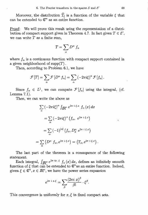
6. The Fourier transform in the spaces S and S' 69

Moreover, the distribution T< is a function of the variable ~ that can be extended to (Un as an entire function.

Proof: We will prove this result using the representation of a distribution of compact support given in Theorem 4.7. In fact given TE[', we can write T as a finite sum,

where fa is a continuous function with compact support contained in a given neighborhood of supp(T) .

Then, according to Problem 6.1, we have

.F [T] = L .F [Dª Ía] = L (-21fi~)"' .F [Ja]·

Sin ce fa E L1, we can compute .F [fa] using the integral, ( cf. Lemma 7.1).

Then, we can write the above as

E (-21fi~)"' Jm: e2" i <x fa (x) dx a

=E (-21fi~)"' (fa, e2" i <x) a

= E(-l)lal (fa,D'; e2"i<.x) a

=E (Dª fa, e2" i <·x) = (Tx, e2" i <·x). a

The last part of the theorem is a consequence of the following statement.

Each integral, Jmn e2" ix. < fa (x) dx, defines an infinitely smooth function of ~ that can be extended to (Unas an entire function. Indeed, given ~ E (i)n, x E IRn, we ha ve the power series expansion

2,,. i x.< = ""(27ri X )l'l . c/3 e ~ ~ ~ .

/3

This convergence is uniformly for x, ~ in fixed compact sets.


Since fa is a continuous function with compact support, we can integrate the series term by term, obtaining:

r e2" i x< Ía (x) dx = "'~ r Ía (x) (27ri x)13 dx t;,13

} JRn L¡- ¡3! } JRn

for every f;, E cvn. This completes the proof of theorem 6.4.#

Remarks 6.1: i) Theorem 6.4 gives part of the following result, called Paley-Wiener

Theorem, (cf. [1], volume 2):

l. Given TES', the following statements are equivalent: a) TE 'D, supp(T) C {x E JRn/lxl ::O: A}. b) f extends to cvn as an entire function and for each N > O,

3 C = C(N) > O such that

if(z)I ::; C (1 lzltN e2"AII=(zJI.

2. 0 Given TES', the following statements are equivalent: a) TE E', supp(T) e {x E JRn/lxl::; A} b) T extends to cvn as an entire function and 3 C, N > O such that

if(z)I ::; C (1 + lzl)N e2"AII=(zJI.

ii) In Chapter 4 we mentioned the possibility of dividing distributions and that this fact would be of interest in the theory of partial differential equations.

Indeed, !et us consider a linear differential operator with constant coefficients,

p (D) = L ª" D", ª" E <V. 1<>1:5 m

Given TES', we can consider

.r [P (D) T] = L ª" (-27rif;,)" .r [T]. 1<>1:5 m

Then, if we denote P (-27rif;,) the polynomial I;1,,1::; m a,, (-27rif;,)", the expression

T=F[ S ] p ( - 27rif;,)

will be a formal solution of the differential equation P (D) T = S.

6. The Fourier transform in the spaces S and S' 71

Laurent Schwartz conjectured, (cf. [1], volmne 2), that every temperate distribution can be divided by any polynomial not identically zero and that the division has at least one result which is also a temperate distribution. This statement was proved by Leon Ehrenpreis, ( cf. [7]).

This implies that the equation P (D) T = S will always have at least one temperate solution, given SES'.

iii) In this Chapter we defined the Fourier transform on S'. However, there are functions, like the exponential elxl, which grow at infinity too fast and thus, do not define temperate distributions. However, using a new space of testing functions, it is possible to define, in the sense of distributions, the Fourier transform of functions that grow rapidly, like elxJ ( cf. [8]).


PROBLEMS

6.1 Given TES', show that

F [(2irix)" T] = Dª F [T].

F[DªT] = (-2iri~)" F[T].

F [T1iT] = e2"t;.h F [T] .

6.2 i) Compute the Fourier transform of the Dirac measure Óa-

ii) Prove that the distributions In lxl and p.v.l belong to S'. Com-x

pute the Fourier transform of p.v.~. How is this Fourier transform related to F [In lxlJ? (cf. Problem 3.2 i)).

iii) Given n/2 < k < n, prove that F [ 1~k] is a function propor-

t . 1 t' 1 10na O ¡i;¡n-k .

Hint: Given a E V, a = 1 on a neighborhood of zero, consider 1 1 1

lxlk = a(x) lxlk + (l - a(x)) lxlk"

6.3 Given TE E', show that the function F [T] belongs to OM, (cf. Problem 4.7). Also, show that its extension to q:n is a function of exponential type.

6.4 Given f ES, show that 3 a constant C >O, only depending on the dimension n of mn' such that

11 f llv ~ C L llnª~lv · l«l~n+l

j,

CHAPTER 7

The L1 and L2 theories of the Fourier transform ( Conclusion)

In this Chapter we will complete the results stated without proof in Chapter 5.

Lemma 7.1: Given f E L1 , we have in the sense of S'

:F [T¡] = T¡

with a similar result for :F.

Proof: Both sides of the equality we want to prove belong to S'. Then, given <p ES, we can write

And also,

(:F[T¡], <p) = j f(x){(J(x)dx.

Thus, we need to show that

J r J e21fix( f (x) dx] 'P (~) d~ = J f (x) [ J e2

1fix<'P (~) d~] dx.

IEC !Jn IR" IR"

But, since the double integral,

J J e21fix.< f (x) 'P (~) dx ~ IRn IR"

exists, Fubini's theorem implies that the iterated integrals coincide. This completes the proof of Lemma 7.1.#

Proof of Theorem 5.4: Given f E L1, we assume that g = :F [f] E

L1. Then, according to Lemma 7.1, we have, using the inversion

73


formula for the Fourier transform in S',

Ty¡9¡ = F[T9 ] = F [r¡] = FF[T¡] = T¡.

Then, according to Theorem 1.4, we conclude that F [g] = f a.e. This completes the proof of Theorem 5.4.#

~oof of Theorem 5.5: We will show that given f E L1 such that f = O a.e., then also f = O a.e.

In fact, using again the above lemma and the inversion formula, we have

T¡=FF[T¡]=F[r¡] =0.

Thus, Theorem 1.4 implies that f = O a.e. This completes the proof of Theorem 5.5.#

Proof of Theorem 5.6: Given <p ES, we know that rp E L2• We want

to show that

110llL2 = ll'PllL' · If we accept that given any <p, 1/; E S we have

(7.1)

then, using (7.1) with 1/; = rp and using the inversion formula for the Fourier transform in S, we obtain

([j5, rp)L' = (<p, .r[rpl)L' = (<p, 'P)L'.

Now, let us prove (7.1).

J ( J e2"ix.<<p(x)dx) 1/;(f;)d!; IR:' IRn

= J 'P (x) { J e-2rrii;.x"I/;(!;) df;)dx. JRn \¡kn

= J e2rrii;.x<p(x)-;¡J(f;)dx df; IR"


Lemma 7.2 : Given f E L2, we have in the sense of S',

F [T¡] = T¡

with a similar result for F.

7. Fourier transform: L1, L2 theories (Conclusion) 75

Proof : Both sides of the equality we want to prove belong to S'. Now, let {cpJ} e S be a sequence such that cpJ·-+ fin L2 as j-+ oo. Then, given cp ES, we have

= lim (Tt¡;,, cp) = lim J <íi;(~)cp(~)d~ = J-+00 J-+00 mn

= lim J 'PJ (x) i;? (x) dx = .lim (T"'f' <;?) = ;-+oo mn J->oo

= (T¡, i;?) = (F [T¡], cp).

This completes the proof of Lemma 7.2.#

Proof of Theorem 5. 7 : It is similar to the proof of Theorem 5.4, but this time we will use Lemma 7.2.

Given f E L 2, let g = ? Then,

Ty¡gj = .r [Tg] = .r [rr] = .r.r [T¡] = T¡.

We can prove in the same way that

.r .r [!] =f.

Now, to show Plancherel identity, we will use (7.1).

Let { 7,b2} e S be a sequence converging to h in L 2. Then, F ['l/;2] -+ f2 in L 2•

Thus, from

(cp, .F['l/;Jl)L' = (<;?, 'l/;j)L' j = 1,2, ...

taking limit as j -+ oo, we obtain

(cp, Í2)L' = (¡p, h) L', 'i 'PE S.

Now, let us considera sequence {'PJ} e S converging to fi in L 2 •

We have

j = 1,2, ...

Thus, ta.king again limit as j -+ oo, we get

(ji, f2)L' = (J;, h) L'.

This proves Plancherel identity, and completes the proof of Theorem 5.7.#

76 Distribution theory and Fourier 'fransform

PROBLEMS

7.1 Given f E L1 n L 2 , show that its Fourier transform computed in the L1 sense, coincides with its Fourier transform computed in the L 2 sense.

7.2 Given f E L1, show that

!= lim r e-2 7rix< f(~) d~ R->oo jl<IS R

in the sense of S'.

CHAPTER 8

The action of Fourier transform on convolution products and multiplicative products.

We know already that the space S is an algebra with both, the convolution product and the multiplicative product, (cf. Problems 2.5). We will now show that the Fourier transform maps one structure into the other.

Lemma 8.1: Given <p,'lj; E S we have

(8.1) :F ['P :F ['lf;l] = :F [cp] * 'lj; and also

(8.2)

Proof: We will prove the fust equality, the proof for the second one being the same.

:F[<p:F['lf;l] =Je2><iz<cp(~) [f c2><ii;x'lj;(x) dx] d~

= J [J e2" i(z-x){ 'P (~) 'lj; (x) dx] d~.

Since the double integral exists, because 'P (~) 'lj; (x) E L1 (mn X mn), we can exchange the order of integration, to obtain

j 'tf;(x) [! e2"i(z-x)i; <p(~)d~] dx=:F(<p) *'lj;.


Remarks 8.1: · i) If we substitute in (8.1) 'lj; by :F ('tf;), we obtain

:F [<p.'lj;] = :F [cp] * :F ['lf;].

Substituting in (8.2) 'lj; by :F ['lf;], we obtain

:F [<p.'lj;] = :F ['P] * :F ['lf;].

ii) If we substitute in (8.2) <p by :F [<p], we obtain

77


Taking the Fourier transform on both sides we get

F ['P * ,,P] = F [<p] · F [,,P].

Ifwe substitute in (8.1) <p by F[<p], we have

F [F [<p] · F [,,Pl] = <p *,P.

Taking this time the conjugate Fourier transform on both sides, we obtain

Theorem 8.1: Given f, g E L1, we have

(8.3) · F[f * g] = F[f] · F [g].

Analogously for F.

Proof: We just proved (8.3) when f, g E S. Now, if f, g E L1, we can find sequences {'Pj}, {,,P;} e S such that

'Pj -+ f and ,,Pj -+ g in L 1 as j -+ oo. Young's Theorem shows that then

'Pj * ,,Pj -+ f * g in L 1 as j -+ oo.

Finally, using Theorem 5.1, we have

F [f * g] (.;) = lim F ['Pj * ,,Pj] (.;) J-->OO

= lim éh (.;);¡Jj (.;) = J(.;) · ?(0, J-->OO

where the limits are uniform limits. This completes the proof of Theorem 8.1.#

Remark 8.2: Theorem 8.1 shows that the Fourier transform is a homomorphism ofthe algebra (L1, *) into the algebra (Co, ·) where Co = {f : IRn -+ (]) / f is continuous and vanishes at infinity} and · denotes the pointwise multiplication.

According to Remarks 5.1 ii), the image of this homomorphism is a proper subalgebra of Co· Moreover, it can be shown that it is a dense

8. Action of Fourier transform on products 79

subalgebra, ( cf. [3], volume 2).

Given distributions T E t:', S E S', the convolution product T * S is well defined as a tempera te distribution, ( cf. Problem 4.2 ii)). Furthermore,

Theorem 8.2: Given T E t:', S E S', we have

(8.4) F[T * S] = F[T] · F[S]

in the sense of S'.

Proof: According to Problems 4. 7 and 6.3, the multiplicative product in the right hand side of ( 8.4) is well defined.

Using now the representation formulas given in Theorems 3.4 and 4.7, we can write

S = Dllg, with g a continuous function slowly increasing. T = '¿; D°' fa, with each fa a continuous function with compact

support. Thus, in the sense of S' we have

F [T * S] = L (-21fi~)"+/J F [T¡0 * Tg].

Now, given <p E S, we can write

(F [T¡0 * T9 ], cp) = j (!fa (y) g (x -y) dy) cp(x) dx.

Since the double integral exists we have, with the change of variable X =y+z,

J fa(y)g(z) cp (y+z)dy dz = = J fa (y) g (z) F [e2

" i x·y <p (x)] (z) dy dz = J Ía(Y) (F[T9 ] (x), e2"ixy cp(x))dy.

Using the commutativity of the tensor product we can write the expression above as

(.r [T9] (x), j fa (y) e2" i x·y dy cp (x)) = (J:. T9 , cp) .

Thus, we conclude that (T * sy = T. s. This concludes the proof of Theorem 8.2.#


PROBLEMS

8.1 Given TE S~, S E S~ , show that T 03 belongs S~ Y and that

F[T0 S] = F[T] 0 F[S]

in the sense of S~ y·

Hint: Use Theorem 3.4.

CHAPTER 9

The Hausdorff - Young theorem

According to what we have seen in Chapters 5 and 7, the Fourier transform is a continuous operator from L1 to L''° and from L 2 onto itself.

On the other hand, we know that V e S', V 1 :S: p :S: oo, (cf. Problem 2.6 iv)). Thus, the Fourier transform is well defined on every V space, 1 :S: p :S: oo, in the sense of S'. Furthermore, the result known as Hausdorff-Young theorem shows that given f E V, 1 :S: p :S: 2, its Fourier transform J in the S' sense , is indeed a function in the space Lq, where ~ + ~ = l. This result is optima!, in the sense that given p > 2, it is possible to find f E V such that its Fourier transform does not belong to Lq, (cf. [9], p. 263).

Theorem 9.1: (Hausdorff-Young): Given f E V, 1 :S: p :S: 2, its Fourier transform J in the sense of S', is a function in the space Lª, l + l = l. Moreover, p q

Befare proving this theorem, we will state and prove two auxiliary results.

Lemma 9.1: (Lindeloff principie): Given a,b E IR, a< b, !et B = {z E©/ a:<; Re z :<; b} and !et 8B be the boundary of B. Then, given any function F (z) bounded and analytic on B, we have

sup IF (z)I = sup IF (z)I. zEB &B

Proof: Given n E IN, n > lal, lbl, !et Fn (z) - :_(~. Then the function Fn is analytic on B. Moreover, since

n IFn (z)I :S: I I sup IF (z)I,

n + Z zEB ZE B

81

' 1

82 Distribution theory and Fouríer Transform

we deduce that

JFn (z)I-+ O as lzl-+ oo, z E B.

Let

Mn = sup JFn (z)I. zEB

Then, exists Nn > O such that

1

Mn JFn (z) ::; 2

Thus, given z E B we have

IFn (z)I ::; sup IFn (z)I ::; sup JFn (z)J. zEB zEB1 ]Jm z¡:::; Nn

Using the maximum principie in the compact domain

En= {z E B/IImzl::; Nn},

the above will be equal to

sup IFn (z)I = sup IFn (z)J zE&Bn zE&Bn, Re z=a orRez=b

::; n-m:Clal,lbll zs~IJ, IFn (z)I.

In the end, we have obtained the estímate n

IFn (z)J ::; (I I lbl) sup IF (z)I n - max a , zEiJB

for any z E B. Thus, taking the limitas n-+ oo, we obtain

s.up IF (z)I ::; sup IF (z)J. zEB zEOB


To state our second auxiliary result, we need to precise the notion of step function.

A function will be called a step function if it can be written as

LAj XP; j=l

where Aj E <V, XP; denotes the characteristic function of an n-dimensional "rectangle" Pj and the family {Pj} is disjoint.

9. The Hausdorff - Young theorem 83

Lemma 9.2: Let f E Lqloc' 1 < q :S oo, and let ~ + ~ = l. Then, the following statements are equivalent

i) f E Lq.

ii) sup J f(x)g(x)dx < oo gES, ll9llLP =l JRn

where s = {g : mn --+ (f, / g is a step function}.

Proof : i) =? ii) Let us consider the linear and continuous map L,

V+--"° S.!+ (f,

g--+ J f(x)g(x)dx.

According to the Hahn - Banach theorem the functional L can be extended to V without changing the norm. Furthermore, the topological dual of IJ' can be identified with Lq, meaning that given any linear and continuous form L on IJ', it can be represented as

L (g) = j f(x)g(x)dx JRn

for sorne f E Lq. Moreover the map

L--+ f

is an onto isometry. Thus, in our case, we will have

Slip ¡r nf(x)g(x)dxl=llfllL,<oo. gES, ll9lb =l ÍJR

ii)=? i) Given k = 1, 2, ... , Jet Bk = { x E !Rn / 11 xll 00 :S k} and Jet Xk be the characteristic function of B k.

Then, there exists 1

lim ( { lxk(x) f (x)l9 dx) ;¡ = 11 f llL, · k -+oo }m,n

We want to show that the limit above is finite. Let us consider again S = {g : !Rn --+ <r, / g is a step function} . Let

us consider for each k = 1, 2, ... the map Lk,

V +--"° S !:!+ (f,

g --+ f mn f (x) Xk (x) g (x) dx.


Holder's inequality shows that this is a continuous functional on S. Again, the Hahn-Banach theorem implies that this functional can be extended to IJ' without changing the norm.

The same duality result mentioned above, gives that

11 ÍXkllL, = 11 Lkll = sup IJ f (x) Xk (x) g (x) dxl. gES, 11 gilLP = 1

Given a step function g, with ll9llLP = 1, we can write by definition,

l

Xk (X) 9 (X) = L Aj XP; n Bk (X) . j=l

This is again a step function. Moreover, l l

11 Xk 9llip = L J.>.jlp IPj n Bkl :::: L J.>.jlp IPjl = L j=l j=l

Thus,

IJ f (x) Xk (x) g (x) dx[ :S: IJ f (x) ~~~x~u~:)dxl

:::; sup IJ f (x) g (x) dx[. gES, !191\cP =1

Since this supremum is finite by hypothesis, we conclude that 3 e > o such that

11 f XkllL, :S: C, V k = 1,2, ...

Thus, f E Lq. This completes the proof of Lemma 9. 2.#

Remark 9.1: As a consequence of the proof of Lemma 9.2, we have

JIJIJLP = sup 1 { "f (x) g (x) dx/. gES, ll9lb =1 J IR

Proof of Theorem 9.1: We will first prove the theorem assuming that the function f is a step function. A density argument will then extend the result to any function in IJ'.

If f is a step function, then f E L1 and its Fourier transform is defined by the integral. According to Lemma 9.2, the function f will

9. The Hausdorff - Young theorem

belong to Lq and 11 J llL,:::; 11 f llLP if we can show that

sup 11 J (x) g (x) dxl :::; 11 f llLP. gES, 11 glb =1

Given z = a + i/3 E <V, we consider the function

Íz = 1 flpz eiArg f,

85

where Arg f denotes the function y --+principal argument of the complex number f (y) when f (y)=/= O and y--+ O if f (y)= O.

The function fz is measurable. Moreover, since lfzl = IJIP", we also have that fz E L1

. Then,

Jz (x) = { e2" ix·y lf (y)lpz ei Argf (y)dy. ÍJR"

l

Since f = E Aj XP;, with { P;} disjoint, we have j=l

l

IJlpz = L IAJlpz XP;,

j=l

which is well defined because 1Aj1 > O, 'ef j. Thus,

l

1z (x) = L IAjlpz J, n e2" ix·y ei Argf (y)XP; (y) dy. j=l IR

From this representation for Jz, we deduce that the function z --+ Jz ( x) is en tire, for each x E IRn fixed.

Given now any step function g with llgllLP = 1, we also consider the function

s

9z = lglpz ei Arg g = L lµrlpz XQ, . ei Arg g. r =l

Now, let

<I?(z) = fJR" Jz (x)gz (x)dx = l s

= E E IAjlpz lµrlpz fq, é Arg g (x) fpj e2" ix·y ei Argf (Yldydx. J=l r =l

This representation shows that <I? is entire function.


Moreover, since l (z)I SI:; IAjlpz lµrlpz IQrl IP;I, where IQrl, IP,I j, r

denote volume, we can deduce that the function (z) is bounded on any region B = {a+i/3 E <r/a S a S b}.

On other hand, when z = ~' fz coincides with f and 9z coincides with g.

When 1 S p S 2, the variable z will belong to the region

B = {a+ if3 E <r / ~ S a S 1} . Now suppose we show that when Re z = ~ and when Re z = 1

the function (z) satisfiesl (z)I S llJllLP. Then, according to Lemma 9.1, we can conclude that l(x)I <

11 f llLP for any z with ~ S Re z S l. Particularly, if 1 S p S 2, we will have

11 f (x)g(x)dxl = l (~)! S 11 f llLP

which is the result we want for a step function f. Thus, !et us show that l (z)I S 11 f llLP if Re z = ~ and if Re

z =l. Suppose first that Re z = ~. Then, we have lfzl = lfl~, l9zl =

lgl ~. Thus, Schwarz inequality and Parseval identity, ( cf. Chapter 5), imply that

1

l (z)I S 11 izllu 119zllu=11 fzllu 11 9zllu = (J lf (y)IP dx) 2

.

Analogously, if Re z = 1, we have 1 fzl = 1 JIP and l9zl = lglP·

Moreover, l.Tzl (x) S f lf(y)IPdy. Thus,

l (z)I S J liz (x)l l9z (x)I dx S J lf (y)IP dy · J lg (x)PI dx

= J lf (y)lp dy.

If we now suppose that 11 f llLP = 1, we have l (z)I S 1 for Re z = ~ and Re z = 1 and thus,

!J J(x) g (x) dxl = l (~) 1 S l.

Finally, if f is any non identically zero step function, we have

9. The Hausdorff - Young theorem 87

Let us now consider any function f E IY and let {fj} be a sequence of step functions such that fj -+ f in V as j -+ oo .

We have,

11 Jj - IillM :S 11 fj - fdlLP-+ Ü as j, l-+ OO.

Then, 3 FE Lq such that Jj-+ Fin Lq. We claim that in the sense of S', F coincides with f. Indeed, since J;P '-+ S', 'ef 1 :S p :S oo, (cf. Problem 2.6 iv)), given

<p E S, we can write

(F, ip) = lim (Jj, ip) = lim (fj, ij5) = (!, ij5). J-+00 ]400

Concerning the norm inequality,

11 .fil = 11 FllL, = lim 11 J;ll :S lim 11 fjllLv = 11 JllLP · I 1 Lq J-+OO L9 J-+oo


Bibliography

[l J Schwartz, L.: "Théorie des distributions, 1,2". Hermann, {1951).

[2] Garvoux, J.: "Espaces vectoriels topologiques et distributions". Dunod, {1963).

[3] Cotlar, M. and Cignoli, R.: "Nociones de espacios normados, 1,2,". Editorial Universitaria de Buenos Aires, (1961).

[4] Bachman, G. and Narici, L.: "Functional Analysis". Academic Press, {1966}.

[5] Gnnning, R. and Rossi, H.: "Analytic functions of severa] complex variables". Prentice-Hall, {1965 ).

[6] Schwartz, L.: "Sur l' impossibilité de la multiplication des distributions". C. R. Acad. Sci. Paris 239, {1954), 841-848.

[7] Ehrenpreis, L.: "Solutions of sorne problems of division". Am. J. Math. 16, {1954), 883-903.

[8] Guelfand, I. and Chilov, G.: "Les distributions". Dunod, {1962).

[9] Donoghue, W. F.: "Distributions and Fourier transforms". Academic Press, (1969}.

89

Documents

Lolina Alvarez Alonso - cms.dm.uba.arcms.dm.uba.ar/.../Distribution-Theory-Lolina.pdf · solutions of partial differential equations and further incorporated the methods of functional