LOKENATH BABA Some Network Optimization Models under

LOKENATH BABA

Some Network Optimization Models under Diverse

Uncertain Environments

A thesis submitted for partial fulfilment of the requirements for the degree of

Doctor of Philosophy

in

Computer Science and Engineering

by

Saibal Majumder

Roll No.: 15/CSE/1101, FT, PhD

Registration No.: NITD/PhD/CS/2016/00742

Under the joint supervision of

Tandra Pal

Professor, Department of Computer Science and Engineering

National Institute of Technology Durgapur, India

and

Samarjit Kar

Professor, Department of Mathematics

National Institute of Technology Durgapur, India

Department of Computer Science and Engineering

National Institute of Technology Durgapur

Durgapur 713209, India

March, 2019

ii

User

Text Box

iii

Dedicated To

My parents, who brought me up and without whom I would not

have come this far.

My respected professors, whose constant guidance motivated me

to remain focused on achieving my goal.

Millions of poor and downtrodden people of my country, whose

sacrifice and tolerance paved the royal road of my education.

User

Text Box

iv

User

Text Box

v

National Institute of Technology

Durgapur

CERTIFICATE

It is certified that the work contained in the thesis entitled “Some Network

Optimization Models under Diverse Uncertain Environments”, has been carried out

by Saibal Majumder (Roll No.: 15/CSE/1101, FT, PhD and Registration No.:

NITD/PhD/CS/2016/00742) under the guidance of Prof. Tandra Pal and Prof.

Samarjit Kar, the data reported herein is original and this work has not been submitted

elsewhere for any other Degree or Diploma.

--------------------------------------

Saibal Majumder (Candidate)

Place: ………………………….

Date: …………………………..

This is to certify that the above declaration is true.

--------------------------------------- ----------------------------------------

Prof. Tandra Pal Prof. Samarjit Kar

Place: …………………………. Place: ………………………….

Date: ………………………….. Date: …………………………..

User

Text Box

vi

User

Text Box

vii

Acknowledgement

Firstly, I pay deep reverence to the Almighty to have bestowed on me, courage and

zeal, to cope up with the challenges in my research. I take this opportunity to express

my deep sense of gratitude and respectful regards to all of those people without whose

support; the thesis would never have been possible. Since it is impossible to name all

of these wonderful people, I will only attempt to mention here a handful of them.

I feel privileged and honour to express my sincere and deepest gratitude to my

supervisors, Prof. Tandra Pal and Prof. Samarjit Kar for their invaluable guidance and

incessant support during my doctoral research endeavour for the past five years. They

have gone beyond their duties to elucidate my doubts, concerns and anxieties, and have

helped me to foster the knowledge required for me. I feel fortunate having them as my

supervisors.

My heartfelt thank goes to the members of my Doctoral Scrutiny Committee including

Prof. G. Sanyal, Prof. S. Roy, Dr. S. Mukhopadhyay and Prof. S. Nandi for providing

me insightful comments and timely directions. My earnest thank also goes to all other

faculty members of the Department of Computer Science and Engineering, National

Institute of Technology Durgapur, for their kind supports throughout my PhD tenure.

The support and cooperation which I have received from my friends are invaluable. I

greatly appreciate and acknowledge the necessary support provided by the departments

of Computer Science and Engineering and Mathematics, National Institute of

Technology Durgapur, to carry out my research work. I extend my thanks to the

academic staffs of the institution for their kind cooperation. A special mention of thanks

is due to Dr. Pradip Kundu, Dr. Sujit Das, Dr. Prasenjit Dey, Dr. Mohuya B. Kar and

Mr. Haresh Sharma for their limitless mental support and cooperation throughout the

course. I am extremely thankful to Dr. Kaustuv Nag for his important suggestion which

is instrumental in my study.

Being an INSPIRE fellow (DST/INSPIRE Fellowship/2015/IF150410), I am indebted

to the Department of Science & Technology (DST), Government of India, for providing

me financial support for my PhD work.

A special thanks to my younger brother Bidyut for his love, affection and active

support.

Finally, I acknowledge my parents and my aunt for giving me the liberty to select what

I desired, and inspiring me to work hard for those I aspire to achieve. I salute you all

User

Text Box

viii

for giving me unconditional love and the sacrifice you did during the journey to fulfil

my dream and aspiration.

Date: Saibal Majumder

Roll No.: 15/CSE/1101, FT, PhD

Registration No.: NITD/PhD/CS/2016/00742

Department of Computer Science and Engineering

National Institute of Technology Durgapur

West Bengal-713209, India

ix

Table of Contents

CERTIFICATE ............................................................................................................. v

Acknowledgement ....................................................................................................... vii

Table of Contents ......................................................................................................... ix

List of Tables ............................................................................................................. xiii

List of Figures ........................................................................................................... xvii

List of Abbreviations .................................................................................................. xix

Abstract ....................................................................................................................... xxi

Chapter 1 Introduction ................................................................................................. 1

1.1 Literature Study ................................................................................................ 5

1.2 Research Motivation and Objectives .............................................................. 14

1.2.1 Motivation.............................................................................................. 14

1.2.2 Objectives .............................................................................................. 16

1.3 Preliminary Concepts ..................................................................................... 17

1.3.1 Fuzzy Set ............................................................................................... 17

1.3.2 Possibility, Necessity and Credibility Measures ................................... 20

1.3.3 Type-2 Fuzzy Set ................................................................................... 23

1.3.4 Type-2 Fuzzy Variable .......................................................................... 25

1.3.5 Random Fuzzy Variable ........................................................................ 26

1.3.6 Rough Set .............................................................................................. 27

1.3.7 Rough Variable ...................................................................................... 28

1.3.8 Trust Measure of Rough Variable ......................................................... 30

1.3.9 Optimistic and Pessimistic Values of Rough Variable .......................... 31

1.3.10 Rough Fuzzy Variable ......................................................................... 32

1.3.11 Uncertainty Theory .............................................................................. 34

1.3.12 Ordered Weighted Averaging (OWA) Operator ................................. 39

1.3.13 Single objective Optimization ............................................................. 40

1.3.14 Multi-objective Optimization (MOP) .................................................. 40

1.3.15 Classical Multi-objective Solution Techniques ................................... 41

1.3.15.1 Linear Weighted Method .............................................................. 41

1.3.15.2 Epsilon-constraint Method ............................................................ 42

User

Text Box

x

1.3.15.3 Goal Attainment Method .............................................................. 42

1.3.15.4 Fuzzy Programming Method ........................................................ 43

1.3.15.5 Global Criterion Method ............................................................... 43

1.3.16 Genetic Algorithms .............................................................................. 44

1.3.16.1 Nondominated Sorting Genetic Algorithm II (NSGA-II) ............. 46

1.3.16.2 Multi-objective Cross Generational Elitist Selection,

Heterogeneous Recombination and Cataclysmic Mutation

(MOCHC) ...................................................................................... 47

1.3.17 Performance Metrics ............................................................................ 48

1.3.17.1 Hypervolume................................................................................. 48

1.3.17.2 Spread ........................................................................................... 48

1.3.17.3 Generational Distance ................................................................... 49

1.3.17.4 Inverted Generational Distance..................................................... 49

1.4 Scope of the Thesis......................................................................................... 50

1.4.1 Introduction............................................................................................ 50

1.4.2 Linear Programming Model with Interval Type-2 Fuzzy Parameters and

its Application to some Network Problems ............................................ 50

1.4.3 Genetic Algorithm with Varying Population for Random Fuzzy

Maximum Flow Problem ........................................................................ 50

1.4.4 Multi-criteria Shortest Path Problem on Rough Graph ......................... 51

1.4.5 Uncertain Multi-objective Multi-item Fixed Charge Solid

Transportation Problem with Budget Constraint .................................... 51

1.4.6 Multi-objective Rough Fuzzy Quadratic Minimum Spanning Tree

Problem ................................................................................................... 52

1.4.7 Conclusion and Future Scope ................................................................ 52

Part-I............................................................................................................................ 53

Chapter 2 Linear Programming Model with Interval Type-2 Fuzzy Parameters and

its Application to some Network Problems................................................................. 55

2.1 Introduction .................................................................................................... 57

2.2 Credibility Measure on Generalized Trapezoidal Fuzzy Variable ................. 59

2.3 Chance-constrained Model (CCM) to Solve LPP .......................................... 60

2.3.1 Chance-constrained Model with Interval Type-2 Fuzzy Constraints .... 61

2.3.2 Chance-constrained Model with Interval Type-2 Fuzzy Objective ....... 63

2.4 Formulation of CCM for STP with Availabilities, Demands and Conveyance

Capacities as IT2FVs ...................................................................................... 65

2.5 Formulation of CCM for SPP and MSTP with Interval Type-2 Fuzzy

Parameters....................................................................................................... 68

2.5.1 CCM for SPP with Interval Type-2 Fuzzy Parameters ......................... 68

xi

2.5.2 CCM for MSTP with Interval Type-2 Fuzzy Parameters ...................... 70

2.6 Numerical Illustrations ................................................................................... 72

2.6.1 STP with Availabilities, Demands and Conveyance Capacities as

IT2FVs .................................................................................................... 72

2.6.2 SPP with Interval Type-2 Fuzzy Parameters ......................................... 75

2.6.3 MSTP with Interval Type-2 Fuzzy Parameters ..................................... 78

2.7 Conclusion ...................................................................................................... 80

Chapter 3 Genetic Algorithm with Varying Population for Random Fuzzy

Maximum Flow Problem ............................................................................................ 83

3.1 Introduction .................................................................................................... 85

3.2 Maximum Flow Problem................................................................................ 87

3.2.1 Problem Formulation ............................................................................. 87

3.2.2 Expected Value Model (EVM) .............................................................. 87

3.2.3 Chance-constrained Model (CCM)........................................................ 88

3.3 Crisp Equivalents of EVM and CCM............................................................. 89

3.4 Proposed Genetic Algorithm .......................................................................... 94

3.4.1 Chromosome Representation ................................................................. 96

3.4.2 Population Initialization......................................................................... 96

3.4.3 Fitness Evaluation .................................................................................. 96

3.4.4 Age and Lifetime of Chromosome ........................................................ 98

3.4.5 Crossover ............................................................................................... 99

3.4.6 Mutation ............................................................................................... 101

3.4.7 Selection .............................................................................................. 101

3.4.8 Elitist Selection .................................................................................... 101

3.4.9 Stopping Criteria .................................................................................. 101

3.5 Results and Discussion ................................................................................. 102

3.5.1 Crisp Instances ..................................................................................... 103

3.5.2 Random Fuzzy Instances ..................................................................... 111

3.6 Conclusion .................................................................................................... 116

Part-II ........................................................................................................................ 119

Chapter 4 Multi-criteria Shortest Path Problem on Rough Graph ........................ 121

4.1 Introduction .................................................................................................. 123

4.2 Proposed Modified Rough Dijkstra’s (MRD) Algorithm ............................ 125

4.3 Proposed Multi-criteria Rough Chance-constrained Shortest Path Problem

(MRCCSPP) ................................................................................................. 129

4.4 Numerical Illustration................................................................................... 133


xii

4.6 Conclusion .................................................................................................... 140

Chapter 5 Uncertain Multi-objective Multi-item Fixed Charge Solid Transportation

Problem with Budget Constraint .............................................................................. 143

5.1 Introduction .................................................................................................. 145

5.2 Problem Definition ....................................................................................... 148

5.2.1 Expected Value Model ........................................................................ 151

5.2.2 Chance-constrained Model .................................................................. 152

5.2.3 Dependent Chance-constrained Model (DCCM) ................................ 153

5.3 Crisp Equivalents of the Models .................................................................. 153

5.4 Methodologies for Crisp Equivalence .......................................................... 155

5.4.1 Linear Weighted Method ..................................................................... 155

5.4.2 Global Criterion Method...................................................................... 156

5.4.3 Fuzzy Programming Method ............................................................... 157


5.6 Conclusion .................................................................................................... 163

Chapter 6 Multi-objective Rough Fuzzy Quadratic Minimum Spanning Tree

Problem...................................................................................................................... 165

6.1 Introduction .................................................................................................. 167

6.2 Multi-objective Model with Rough Fuzzy Coefficients............................... 170

6.3 Quadratic Minimum Spanning Tree Problem with Rough Fuzzy Coefficients

...................................................................................................................... 175

6.4 Numerical Illustration................................................................................... 177


6.6 Case Study .................................................................................................... 184

6.7 Conclusion .................................................................................................... 187

Chapter 7 Conclusion and Future Scope ................................................................. 189

7.1 Conclusion .................................................................................................... 191

7.2 Future Scope ................................................................................................. 192

Appendix A ................................................................................................................ 195

Appendix B ................................................................................................................ 199

Appendix C ................................................................................................................ 201

Appendix D ................................................................................................................ 209

Appendix E ................................................................................................................ 213

References ................................................................................................................. 217

List of Publications ................................................................................................... 241

xiii

List of Tables

Table 2.1 Transportation cost of the product from source 𝑖 to destination 𝑗 via

conveyance 𝑘............................................................................................................ 72

Table 2.2 Availability of the product at different sources represented by IT2FV ...... 72

Table 2.3 Demand of the product at different destinations represented by IT2FV .... 72

Table 2.4 Capacity of different types of conveyances represented by IT2FV ............ 73

Table 2.5 Compromise solution generated by the model (2.38) ................................. 74

Table 2.6 Compromise cost of the STP at different predetermined confidence levels

.................................................................................................................................. 75

Table 2.7 Interval type-2 fuzzy edge costs of the WCDN 𝐺 ...................................... 76

Table 2.8 Results generated by models (2.28), (2.30) and (2.31) for the WCDN 𝐺 .. 77

Table 2.9 Compromise cost of the proposed SPP for the WCDN 𝐺 at different

credibility levels ....................................................................................................... 78

Table 2.10 Interval type-2 fuzzy edge costs of the WCUN 𝐻 .................................... 79

Table 2.11 Results generated by models (2.33), (2.34) and (2.35) for the WCUN 𝐻

.................................................................................................................................. 80

Table 2.12 Compromise cost of the proposed MSTP for the WCUN 𝐻 at different

credibility levels ....................................................................................................... 81

Table 3.1 Uncertain rule base for crossover probability 𝜉𝑝𝑐 ..................................... 100

Table 3.2 Parameter setting for experimentation of the algorithms .......................... 104

Table 3.3 𝑚𝑎𝑥 𝑓𝑖𝑡𝑛𝑒𝑠𝑠, 𝑚𝑒𝑎𝑛 𝑓𝑖𝑡𝑛𝑒𝑠𝑠 with 𝑠𝑑 and 𝑚𝑒𝑎𝑛 𝑒𝑥𝑒𝑐𝑢𝑡𝑖𝑜𝑛 𝑡𝑖𝑚𝑒 for the

six instances of maximum flow problem ............................................................... 104

Table 3.4 Performances of the proposed VPGAwIC on the instance 𝑚𝑓𝑙𝑜𝑤_102_290

at different values of 𝑃𝑜𝑝𝑆𝑖𝑧𝑒𝑇ℎ .......................................................................... 105


at different values of 𝜌 ........................................................................................... 106


at different values of 𝑚𝑎𝑥𝐿𝑇 ................................................................................. 106

Table 3.7 Comparison of results for the proposed VPGAwIC with different allocation

strategies for the six instances of maximum flow problem.................................... 107

Table 3.8 Median of maximum fitness of the six instances of maximum flow problem

for the MFGA and proposed VPGAwIC .................................................................. 110

User

Text Box

xiv


for the VPGAwIC-bLAS and VPGAwIC-iLAS ......................................................... 111

Table 3.10 Random fuzzy capacities expressed as TrRFV of the instance

𝑚𝑓𝑙𝑜𝑤_𝑇𝑟𝑅𝐹_10_15 ............................................................................................. 112

Table 3.11 Random fuzzy capacities expressed as GRFV of the instance

𝑚𝑓𝑙𝑜𝑤_𝐺𝑅𝐹_10_15 ............................................................................................... 113

Table 3.12 Comparison of results for crisp equivalents of the EVM and the CCM

.............................................................................................................................. ..113

Table 3.13 Solutions of the model (3.9) at different confidence levels of 𝐶𝑟 and 𝑃𝑟 for

the random fuzzy maximum flow instance 𝑚𝑓𝑙𝑜𝑤_𝑇𝑟𝑅𝐹_10_15 ....................... 115

Table 3.14 Solutions of the model (3.10) at different confidence levels of 𝐶𝑟 and 𝑃𝑟

for the random fuzzy maximum flow instance 𝑚𝑓𝑙𝑜𝑤_𝐺𝑅𝐹_10_15..................... 116

Table 4.1 Edge weights of the WCDN 𝐺: distance, cost and time represented by rough

variable ................................................................................................................... 134

Table 4.2 Pessimistic and optimistic shortest paths of the WCDN 𝐺 when solved by

MRD algorithm ...................................................................................................... 135

Table 4.3 Optimum values for pessimistic models 𝑀5, 𝑀6, 𝑀7 and optimistic models

𝑀11, 𝑀12, 𝑀13 for the WCDN 𝐺 at different trust levels of 𝑇𝑚 ............................ 136

Table 4.4 Optimum results for the models 𝑀′and 𝑀′′ for the WCDN 𝐺 ................. 138

Table 4.5 Compromise objective vectors of the WCDN 𝐺 at different trust levels of

𝑇𝑚 .......................................................................................................................... 138

Table 4.6 Comparisons of results obtained by MRD algorithm and MRCCSPP for the

WCDN 𝐺 ................................................................................................................

Table 4.7 Computation time for MRD algorithm for larger WCDNs with rough

parameters .............................................................................................................. 140

Table 4.8 Statistical measures of 𝐻𝑉 after 15 runs of NSGA-II on the pessimistic

model (4.4) of the WCDNs 𝐺 and 𝑅 ..................................................................... 140

Table 4.9 Statistical measures of 𝐻𝑉 after 15 runs of NSGA-II on the optimistic model

(4.6) of the WCDNs 𝐺 and 𝑅 ................................................................................

Table 4.10 Statistical measures of Δ after 15 runs of NSGA-II on the pessimistic model

(4.4) of the WCDNs 𝐺 and 𝑅 ................................................................................ 141

Table 4.11 Statistical measures of Δ after 15 runs of NSGA-II on the optmistic model

(4.6) of the WCDNs 𝐺 and 𝑅 ................................................................................ 141

Table 4.12 Statistical measures of execution time after 15 runs of NSGA-II on the

pessimistic model (4.4) of the WCDNs 𝐺 and 𝑅 .................................................. 142

141

139

xv


optimistic model (4.6) of the WCDNs 𝐺 and 𝑅 .................................................... 142

Table 5.1 Some recent studies on variants of transportation problem under diverse

uncertain frameworks ............................................................................................. 147

Table 5.2 Optimum results of EVM and CCM for zigzag and normal uncertain

variables using linear weighted method ................................................................. 161

Table 5.3 Comparative results of three different solution methodologies ................ 161

Table 5.4 Optimal transportation plan of the EVM and CCM for normal uncertain

variables using three different solution methodologies ......................................... 162

Table 5.5 Results of DCCM for zigzag and normal uncertain variables .................. 163

Table 5.6 Optimal transportation plan for DCCM for normal uncertain variables... 163

Table 5.7 Results for CCM for zigzag and normal uncertain variables at different

chance levels of 𝛼1 and 𝛼2 ..................................................................................... 164

Table 6.1 Rough fuzzy linear weights of the WCUN 𝐺 ........................................... 178

Table 6.2 Rough fuzzy quadratic weights of the WCUN 𝐺 ..................................... 179

Table 6.3 Solutions of models (6.8) and (6.9) of the WCUN 𝐺 ............................. 179

Table 6.4 Mean and sd of 𝐻𝑉, Δ, 𝐺𝐷 and 𝐼𝐺𝐷 after 100 runs of NSGA-II and MOCHC

on each of the five rough fuzzy instances of QMST at predetermined confidence

levels, 𝛼 = 0.9 and 𝛽 = 0.4 ................................................................................... 183

Table 6.5 Median and 𝐼𝑄𝑅 of 𝐻𝑉, Δ, 𝐺𝐷 and 𝐼𝐺𝐷 after 100 runs of NSGA-II and

MOCHC on each of the five rough fuzzy instances of QMST at predetermined

confidence levels, 𝛼 = 0.9 and 𝛽 = 0.4 ................................................................ 183

Table 6.6 Mean and 𝑠𝑑 of 𝐻𝑉, Δ, 𝐺𝐷 and 𝐼𝐺𝐷 after 100 runs of NSGA-II and MOCHC

on each of the five rough fuzzy instances of QMST at predetermined confidence

levels, 𝛼 = 0.9 and 𝛽 = 0.8 ................................................................................... 184

Table 6.7 Median and 𝐼𝑄𝑅 of 𝐻𝑉, Δ, 𝐺𝐷 and 𝐼𝐺𝐷 after 100 runs of NSGA-II and


confidence levels, 𝛼 = 0.9 and 𝛽 = 0.8 ................................................................ 185

Table 6.8 A compromise solution of the model (6.9) for the WCUN 𝑊 ................ 186

Table A.1 Edge costs of 𝑆 estimated by experts ....................................................... 195

Table A.2 Edge weights of 𝑅: distance, cost and time represented by rough variable

................................................................................................................................ 196

Table D.1 Unit purchase costs of items 1 and 2 at two different sources ................. 209

Table D.2 Unit selling prices of items 1 and 2 at three different destinations .......... 209

xvi

Table D.3 Transportation cost for item 1 and item 2 represented by zigzag and normal

uncertain variables ................................................................................................. 209

Table D.4 Fixed charge cost for item 1 and item 2 represented by zigzag and normal


Table D.5 Transportation time for item 1 and item 2 represented by zigzag and normal


Table D.6 Available amounts of item 1 and item 2 represented by zigzag and normal


Table D.7 Demand for item 1 and item 2 represented by zigzag and normal uncertain

variables ................................................................................................................. 211

Table D.8 Transportation capacities of two conveyances expressed as zigzag and

normal uncertain variables ..................................................................................... 211

Table D.9 Budget availability at destinations represented by zigzag and normal


Table E.1 The rough fuzzy linear weights representing the possible costs to the

company while providing the air service between a pair of cities ......................... 213

Table E.2 The rough fuzzy quadratic weights of a pair of adjacent edges representing

the possible discount on the total flight fare of two consecutive flights ................ 214

Table E.3 Continuation of Table E.2 ........................................................................ 215

xvii

List of Figures

Figure 1.1 Membership function of the TrFN 휁 = 𝒯𝑟(4,6,9,11) ............................... 18

Figure 1.2 Membership function of the TFN 휂 = 𝒯(6,8,10) ..................................... 19

Figure 1.3 Membership function of the GFN 𝜉 = 𝒩(5, 2) ........................................ 19

Figure 1.4 Interval type-2 fuzzy set �� ......................................................................... 24

Figure 1.5 Graphical interpretation of the TrIT2FV �� ............................................... 25

Figure 1.6 A rough set 𝑆 ............................................................................................. 28

Figure 1.7 Trust distribution of a rough event 휁 ≤ 𝑟 .................................................. 33

Figure 1.8 Trust distribution of a rough event 휁 ≥ 𝑟 ................................................. 34

Figure 1.9 Linear uncertain distribution of ℒ(6,14) .................................................. 35

Figure 1.10 Zigzag uncertain distribution of 𝒵(10,12,17) ....................................... 36

Figure 1.11 Normal uncertain distribution of 𝒩(10,2) ............................................ 36

Figure 1.12 𝐻𝑉 for different optimized fronts 𝑆1 and 𝑆2 with respect to a reference

solution 𝑅. (a) The front 𝑆1 is closer to PF than 𝑆2, hence shall have higher 𝐻𝑉 (b)

The front 𝑆2 is more diversely spread than 𝑆1, hence shall have higher 𝐻𝑉 .......... 49

Figure 2.1 Compromise transportation cost for the proposed STP generated by solving

model (2.25) at different confidence levels.............................................................. 74

Figure 2.2 A WCDN 𝐺 with interval type-2 fuzzy edge costs ................................... 75

Figure 2.3 Compromise cost of the WCDN 𝐺 generated by solving model (2.31) at

different confidence levels ....................................................................................... 77

Figure 2.4 A WCUN 𝐻 with interval type-2 fuzzy edge costs ................................... 79

Figure 2.5 Compromise cost of the WCUN 𝐻 generated by solving model (2.35) at

different confidence levels ....................................................................................... 81

Figure 3.1 Uncertainty distributions of chromosome’s age ........................................ 99

Figure 3.2 Uncertainty distributions of crossover probability 𝜉𝑝𝑐 ............................ 100

Figure 3.3 Convergence plots of MFGA, VPGAwIC-bLAS and VPGAwIC-iLAS for the

maximum flow instances: (a) 𝑚𝑓𝑙𝑜𝑤_102_290 (b) 𝑚𝑓𝑙𝑜𝑤_902_2670 and (c)

𝑚𝑓𝑙𝑜𝑤_2502_7450 ............................................................................................... 108

Figure 3.4 Boxplots of the maximum flow instances: (a)

𝑚𝑓𝑙𝑜𝑤_11_22 (b) 𝑚𝑓𝑙𝑜𝑤_25_49 (c) 𝑚𝑓𝑙𝑜𝑤_20_300 (d) 𝑚𝑓𝑙𝑜𝑤_102_290 (e)

𝑚𝑓𝑙𝑜𝑤_902_2670 and (f) 𝑚𝑓𝑙𝑜𝑤_2502_7450 ................................................... 110

User

Text Box

xviii

Figure 3.5 A directed connected network 𝐺 ............................................................. 112

Figure 3.6 Convergence plot of the proposed VPGAwIC for the random fuzzy

maximum flow instances: (a) 𝑚𝑓𝑙𝑜𝑤_𝑇𝑟𝑅𝐹_10_15 using model (3.7)

(b) 𝑚𝑓𝑙𝑜𝑤_𝑇𝑟𝑅𝐹_10_15 using model (3.9) (c) 𝑚𝑓𝑙𝑜𝑤_𝐺𝑅𝐹_10_15 using

model (3.8) (d) 𝑚𝑓𝑙𝑜𝑤_𝐺𝑅𝐹_10_15 using model (3.10) ................................... 115

Figure 4.1 A weighted connected directed network 𝐺 .............................................. 134

Figure 4.2 Nondominated solutions of the WCDN 𝐺 by solving the corresponding (a)

pessimistic shortest path model (4.4) at 0.45 trust level (b) optimistic shortest path

model (4.6) at 0.45 trust level (c) pessimistic shortest path model (4.4) at 0.85 trust

level (d) optimistic shortest path model (4.6) at 0.85 trust level ........................... 137

Figure 5.1 Graphical representation of UMMFSTPwB: from model formulation to

solution techniques ................................................................................................. 151

Figure 5.2 Uncertainty distribution of CCM at different chance levels of 𝛼1 and 𝛼2, for

(a) zigzag uncertain variables (b) normal uncertain variables ............................... 164

Figure 6.1 A weighted connected undirected network 𝐺 .......................................... 178

Figure 6.2 A rough fuzzy quadratic minimum spanning tree of the WCUN 𝐺 with 𝛼 =

0.9 and 𝛽 = 0.4 ...................................................................................................... 180

Figure 6.3 A rough fuzzy quadratic minimum spanning tree of the WCUN 𝐺 with 𝛼 =

0.9 and 𝛽 = 0.8 ...................................................................................................... 180

Figure 6.4 Nondominated solutions of the model (6.8) for the WCUN 𝐺 at

predetermined confidence levels, 𝛼 = 0.9 and 𝛽 = 0.4 when solved by the epsilon-

constraint method, and (a) NSGA-II and (b) MOCHC .......................................... 181




Figure 6.6 A weighted connected undirected network 𝑊 ........................................ 185

Figure 6.7 Nondominated solutions of the model (6.9) for the WCUN 𝑊 at

predetermined confidence levels, 𝛼 = 0.9 and 𝛽 = 0.8, when solved by the epsilon-


Figure 6.8 A possible flight schedule for the compromise solution of the WCUN 𝑊 as

reported in Table 6.8 .............................................................................................. 187

Figure A.1 A WCDN 𝑆 with associated edge weights represented by rough variable

................................................................................................................................ 195

Figure A.2 A WCDN 𝑅 with associated edge weights represented by rough variable

................................................................................................................................ 197

xix

List of Abbreviations

Table 0.1 test

bLAS Bilinear allocation strategy

b-RFQMSTP bi-objective rough fuzzy quadratic minimum

spanning tree problem

b-SPP bi-objective shortest path problem

CCM Chance-constrained model

CHC Cross generational, elitist selection,

heterogeneous recombination and cataclysmic

mutation

DCCM Dependent chance-constrained model

DCM Dependent-chance model

DM Decision maker

EA Evolutionary algorithm

EVM Expected value model

FOU Footprint of uncertainty

FTP Fixed charge transportation problem

GA Genetic algorithm

𝐺𝐷 Generational distance

GFN Gaussian fuzzy number

GRFV Gaussian random fuzzy variable

GTrFV Generalized trapezoidal fuzzy variable

𝐻𝑉 Hypervolume

𝐼𝐺𝐷 Inverted generational distance

iLAS Improved lifetime allocation strategy

IQR Interquartile range

IT2FS Interval type-2 fuzzy set

IT2FV Interval type-2 fuzzy variable

𝑘-SPP 𝑘-shortest path problem

LMF Lower membership function

LPP Linear programming problem

MCDM Multi-criteria decision making

MFGA Maximum flow genetic algorithm

MFP Maximum flow problem

MMFSTPwB Multi-objective multi-item fixed charge solid

transportation problem with budget constraint

MOCHC Multi-objective cross generational, elitist

selection, heterogeneous recombination and

cataclysmic mutation

MOGA Multi-objective genetic algorithm

MOP Multi-objective optimization problem

User

Text Box

xx

MP Mathematical programming

MRCCSPP Multi-criteria rough chance-constrained shortest

path problem

MRD Modified rough Dijkstra’s

𝑚𝑠 Milliseconds

MSPP Multi-criteria shortest path problem

MST Minimum spanning tree

MSTP Minimum spanning tree problem

NSGA-II Nondominated sorting genetic algorithm II

OSPF Open shortest path first

OWA Ordered weighted averaging

PF Pareto front

PS Pareto set

PSO Particle swarm optimization

QMST Quadratic minimum spanning tree

QMSTP Quadratic minimum spanning tree problem

RCCP Rough chance-constrained programming

RFCCP Rough fuzzy chance-constrained programming

RFMFP Random fuzzy maximum flow problem

RFMOP Rough fuzzy multi-objective problem

𝑠𝑑 Standard deviation

SIFN Symmetrical intuitionistic fuzzy number

SOOP Single objective optimization problem

SPP Shortest path problem

STP Solid transportation problem

T1FS Type-1 fuzzy set

T1FV Type-1 fuzzy variable

T2FS Type-2 fuzzy set

T2FV Type-2 fuzzy variable

TFN Triangular fuzzy number

TP Transportation problem

TrFN Trapezoidal fuzzy number

TrIT2FV Trapezoidal interval type-2 fuzzy variable

TrRFV Trapezoidal random fuzzy variable

UMF Upper membership function

UMMFSTPwB Uncertain multi-objective multi-item fixed

charge solid transportation problem with budget

constraint

VPGAwIC Varying population genetic algorithm with

indeterminate crossover

WCDN Weighted connected directed network

WCN Weighted connected network

WCUN Weighted connected undirected network

xxi

Abstract

Network models provide an efficient way to represent many real-life problems

mathematically. In the last few decades, the field of network optimization has witnessed

an upsurge of interest among researchers and practitioners. The network models

considered in this thesis are broadly classified into four types: (i) transportation

problem, (ii) shortest path problem, (iii) minimum spanning tree problem and (iv)

maximum flow problem.

Quite often, we come across situations, when the decision parameters of network

optimization problems are not precise and characterized by various forms of

uncertainties arising from the factors, like insufficient or incomplete data, lack of

evidence, inappropriate judgements and randomness. Considering the

crisp/deterministic environment, there exist several studies on network optimization

problems. However, in the literature, not many investigations on single and multi-

objective network optimization problems are observed under diverse uncertain

frameworks. This thesis proposes seven different network models under different

uncertain paradigms. Among those, four network models are formulated as single

objective optimization problems and the remaining three network models as multi-

objective optimization problems. To formulate all these network models, we have

considered type-2 fuzzy, random fuzzy, rough, uncertainty theory and rough fuzzy

uncertain environments. Mainly, among the four single objective network models, the

solid transportation problem, the shortest path problem, and the minimum spanning tree

problem are modelled under type-2 fuzzy environment, and the maximum flow problem

is presented under random fuzzy uncertain paradigm. Among the three multi-objective

problems, the multi-objective shortest path problem, the multi-objective multi-item

fixed charge solid transportation problem with budget constraints and the multi-

objective quadratic spanning tree problem are respectively, modelled under rough,

uncertainty theory and rough fuzzy uncertain paradigms. In this thesis, the uncertain

programming techniques used to formulate the uncertain network models are (i)

expected value model, (ii) chance-constrained model and (iii) dependent chance-

constrained model. Subsequently, the corresponding crisp equivalents of the uncertain

network models are solved using different solution methodologies.

The solution methodologies used in this thesis can be broadly categorized as classical

methods and evolutionary algorithms. The classical methods, used in this thesis, are

Dijkstra’s and Kruskal’s algorithms, modified rough Dijkstra’s algorithm, goal

attainment method, linear weighted method, global criterion method, epsilon-constraint

method and fuzzy programming method. Whereas, among the evolutionary algorithms,

we have proposed the varying population genetic algorithm with indeterminate

crossover and considered two multi-objective evolutionary algorithms:

User

Text Box

xxii

(i) nondominated sorting genetic algorithm II and (ii) multi-objective cross generational

elitist selection, heterogeneous recombination, and cataclysmic mutation.

To illustrate the proposed network models, suitable numerical examples are provided

in this thesis. Moreover, the corresponding results of the proposed uncertain network

models are compared and analyzed.

Keywords: Single objective optimization ⋅ Multi-objective optimization ⋅ Expected

value model ⋅ Chance-constrained model ⋅ Dependent chance-constrained model ⋅

Genetic algorithm ⋅ Multi-objective evolutionary algorithm ⋅ Shortest path problem ⋅

Minimum spanning tree problem ⋅ Transportation problem ⋅ Quadratic minimum

spanning tree problem.

1

Chapter 1

Introduction

User

Text Box

2

User

Text Box

3

Chapter 1

Introduction

Network optimization is one of the most frequently encountered class of optimization

techniques which deals with the optimization of several real-life network problems. A

rich contribution in network optimization can be observed in the contemporary fields

of operations research, engineering and management. Most of the problems in these

fields, including communication systems, electrical networks, computer networks,

scheduling problems, shortest paths, maximal flow, shortest tour, supply and demand

problems, etc., can be modelled and solved using graph theory techniques. The genesis

of network optimization has a connection with the famous Königsberg bridge problem

(L. Euler 1736) in graph theory. Network optimization has received remarkable

attention among researchers and practitioners after the appearance of the first book on

graph theory by D. König (1936). In 1941, F.L. Hitchcock presented the first algorithm

to solve the transportation problem. Subsequently, Jr. J.B. Kruskal (1956) proposed the

minimum spanning tree algorithm. In the same year, the first algorithm to solve the

maximum flow problem (Ford and Fulkerson 1956) in a network was proposed. Moving

forward, there has been steady progress in the solution methodologies of network

problems due to the technological advancement of the computer system and the

development of many efficient algorithms. The acceptability of the network

optimization as well as the theoretical significance in the context of complexity theory,

which deals with the analysis of algorithms (D. Jungnickel 1999) have been increased.

Considering the practical relevance of the network applications, several researchers

have contributed to different types of network optimization problems (R.C. Prim 1957;

E.W. Dijkstra 1959; S.E. Dreyfus 1969; Bhatia et al. 1976). All these problems are

usually investigated with deterministic problem parameters. Nevertheless, in many

real-world network problems, the associated parameters are not always exact or precise.

Bellman and Zadeh (1970) mentioned that “Much of the decision making in the real-

world takes place in an environment in which the goals, the constraints and the

consequences of possible actions are not known precisely.” The reasons behind the

existence of uncertainty in the problem parameters are the availability of insufficient

information, lack of evidence, uncertainty in judgment, etc. Therefore, a proper

representation of the uncertain parameters is necessary while modelling real-world

problems. In order to process and represent the imprecise data, many researchers have

proposed different theories, like probability theory, fuzzy set (L.A. Zadeh 1965), type-

2 fuzzy set (L.A. Zadeh 1975a, b), rough set (Z. Pawlak 1982) and uncertainty theory

User

Text Box

4

(B. Liu 2007). In this thesis, while developing different network models, we have used

interval type-2 fuzzy variable (T.-Y. Chen 2013, 2014), random fuzzy variable (B. Liu

2002), rough variable (B. Liu 2002), rough fuzzy variable (B. Liu 2002) and uncertain

variable (B. Liu 2007) to represent the related parameters of different models.

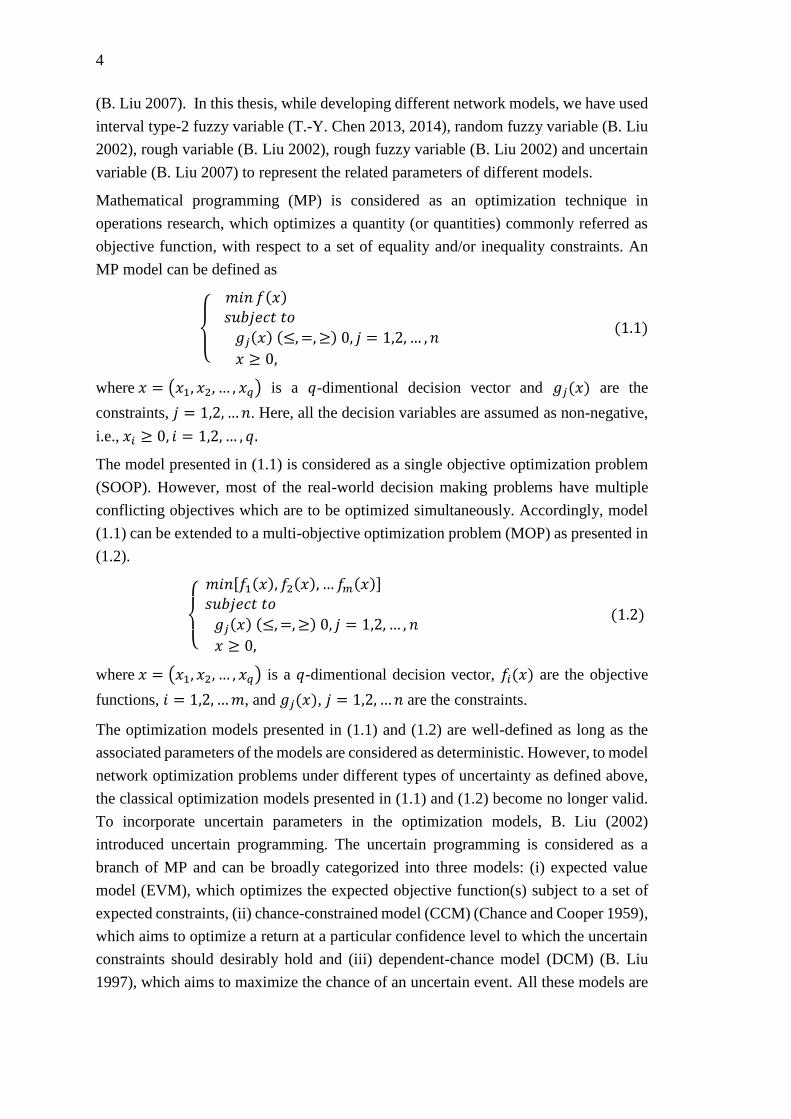
Mathematical programming (MP) is considered as an optimization technique in

operations research, which optimizes a quantity (or quantities) commonly referred as

objective function, with respect to a set of equality and/or inequality constraints. An

MP model can be defined as

{

𝑚𝑖𝑛 𝑓(𝑥) 𝑠𝑢𝑏𝑗𝑒𝑐𝑡 𝑡𝑜

𝑔𝑗(𝑥) (≤,=,≥) 0, 𝑗 = 1,2, … , 𝑛

𝑥 ≥ 0,

(1.1)

where 𝑥 = (𝑥1, 𝑥2, … , 𝑥𝑞) is a 𝑞-dimentional decision vector and 𝑔𝑗(𝑥) are the

constraints, 𝑗 = 1,2, …𝑛. Here, all the decision variables are assumed as non-negative,

i.e., 𝑥𝑖 ≥ 0, 𝑖 = 1,2, … , 𝑞.

The model presented in (1.1) is considered as a single objective optimization problem

(SOOP). However, most of the real-world decision making problems have multiple

conflicting objectives which are to be optimized simultaneously. Accordingly, model

(1.1) can be extended to a multi-objective optimization problem (MOP) as presented in

(1.2).

{

𝑚𝑖𝑛[𝑓1(𝑥), 𝑓2(𝑥), … 𝑓𝑚(𝑥)] 𝑠𝑢𝑏𝑗𝑒𝑐𝑡 𝑡𝑜

𝑔𝑗(𝑥) (≤,=,≥) 0, 𝑗 = 1,2, … , 𝑛

𝑥 ≥ 0,

(1.2)

where 𝑥 = (𝑥1, 𝑥2, … , 𝑥𝑞) is a 𝑞-dimentional decision vector, 𝑓𝑖(𝑥) are the objective

functions, 𝑖 = 1,2, …𝑚, and 𝑔𝑗(𝑥), 𝑗 = 1,2, … 𝑛 are the constraints.

The optimization models presented in (1.1) and (1.2) are well-defined as long as the

associated parameters of the models are considered as deterministic. However, to model

network optimization problems under different types of uncertainty as defined above,

the classical optimization models presented in (1.1) and (1.2) become no longer valid.

To incorporate uncertain parameters in the optimization models, B. Liu (2002)

introduced uncertain programming. The uncertain programming is considered as a

branch of MP and can be broadly categorized into three models: (i) expected value

model (EVM), which optimizes the expected objective function(s) subject to a set of

expected constraints, (ii) chance-constrained model (CCM) (Chance and Cooper 1959),

which aims to optimize a return at a particular confidence level to which the uncertain

constraints should desirably hold and (iii) dependent-chance model (DCM) (B. Liu

1997), which aims to maximize the chance of an uncertain event. All these models are

5

the possible strategies that a decision maker (DM) can adopt while modelling network

problems as uncertain single objective or multi-objective optimization problems.

In the field of optimization, the classical search and optimization techniques are based

on single point search, where a solution is improved with iteration. Some studies on the

classical approaches used to solve single objective network problems (G.B. Dantzig

1951; Ford and Fulkerson 1956; R.C. Prim 1957; E.W. Dijkstra 1959) can be observed

in the literature. Several classical techniques for multi-objective problems, such as

linear weighted method (R.T. Eckenrode 1965), epsilon-constraint method (Haimes et

al. 1971), goal attainment method (F.W.Gembicki 1974), fuzzy programming method

(H.-J. Zimmermann 1978) and global criterion method (S.S. Rao 2006) are observed in

the literature. Sutcliffe et al. (1984), Gupta and Warburton (1987) and Pulat et al. (1992)

have applied some of these techniques on multi-objective network problems. In the

field of optimization, over the last few decades, significant progress in optimization

technique has been observed which are based on evolutionary techniques. An

evolutionary technique is a population based stochastic optimization technique, which

imitates the evolutionary phenomena of nature while driving its search towards

optimality. Unlike classical methods, it generates a set of solutions at each iteration. If

an optimization problem has a single optimum, then all the population members of the

evolutionary methods converge at that optimum. For multiple objectives, it provides

multiple optima in its final population. The inimitable characteristic of evolutionary

techniques to search multiple solutions in a single execution, essentially makes them

unique alternatives to solve MOPs.

In this thesis, we have mainly concentrated on modelling different single and multi-

objective network optimization problems under various uncertain paradigms using

uncertain programming techniques. These problems are then transformed to their crisp

equivalents and are eventually solved using different solutions methodologies, using

both classical and evolutionary algorithms.

1.1 Literature Study

In this section, we present a survey on the studies related to four network optimization

problems: (i) transportation problem, (ii) shortest path problem, (iii) minimum spanning

tree problem and (iv) maximum flow problem, which broadly categorize the

contributions in our thesis. Here, we have also provided brief discussion of the

investigations done on different variants of these network problems. It is to be

mentioned that, this survey, by no means, encompasses all the related researches in the

literature. However, some studies having significant contributions to these network

problems are reviewed below.

6

Transportation problem (TP)

With the development of economic globalization, transportation problem has emerged

as one of the important combinatorial optimization problems and becomes very relevant

to the ever-expanding worldwide market. TP determines an optimal distribution of the

products from each of the sources to various destinations to minimize the total

transportation cost. The problem is first introduced by F.L. Hitchcock (1941) and

subsequently improved by T.C. Koopmans (1949). Following the contributions of their

studies, G.M. Appa (1973) discussed different cases of the unboundedness and

infeasibility of the models of TP. C.S. Ramakrishnan (1988) revisited the problem and

proposed an improved Vogel’s approximation method (Reinfeld and Vogel 1958) as a

solution technique of the TP. Arsham and Kahn (1989) proposed an algorithm for TP,

which is faster than simplex (G.B. Dantzig 1951), more general than stepping-stone

method (W. Shih 1987) and simpler than both. S.I. Gass (1990) analyzed different

facets of solution methodologies of TP. Vignaux and Michalewicz (1991) proposed a

genetic algorithm as a new solution approach to the problem. Considering multi-

objective TP, Aneja and Nair (1979) proposed a parametric search method to solve a

bi-objective TP. H. Isermann (1979) proposed an algorithm to determine the

nondominated solutions to the problem. G.K. Tayi (1986) solved a transportation

problem by minimizing transportation cost and deterioration of an item during a

transportation activity. The author developed an approach by explicitly considering

trade-offs between the objectives as stated by a decision maker.

An important extension of a classical transportation problem is fixed charge

transportation problem, first proposed by Hirsch and Dantzig (1968). In practical

applications, the fixed charge problem may include highway toll charges, landing fees

at airports, cost for construction of roads or setup costs in production system (Palekar

et al. 1990). Kennington and Unger (1976) and Barr et al. (1981) solved the fixed charge

TP with branch-and-bound algorithm. Subsequently, different branch-and-bound

algorithms with conditional penalties are employed by Cabot and Erenguc (1984, 1986)

and Lamar and Wallace (1997), as solution methodologies of the problem. Later,

Adlakha and Kowalski (2003) proposed a heuristic algorithm for the problem. Of late,

Lotfi and Tavakkoli-Moghaddan (2013) proposed a genetic algorithm with priority-

based encoding to solve the problem. Further, Kowalski et al. (2014) developed a

simple branching algorithm to generate a global solution of a fixed charge TP.

Subsequently, a local search algorithm and an artificial immune algorithm were

proposed by Buson et al. (2014) and Altassan et al. (2014), respectively, for solving TP.

The solid transportation problem is yet another variant of the traditional TP. Here, apart

from availability and demand constraints, there is one more constraint known as

conveyance constraint. There may be multiple modes of conveyances, available at the

sources for transporting items. Therefore, the conveyances constraint is used to

7

determine an appropriate mode of transportation so that the total transportation cost is

minimized. In this context, K.B. Haley (1962) first introduced the solid TP. The

problem was again addressed by Hadley and Whitin (1963). Ever since, solid TP has

received much attention among researchers. H.L. Bhatia (1981) determined feasible

solutions of a solid TP with indefinite quadratic objective function. Pandian and

Anuradha (2010) proposed a new method using the principle of zero point method

(Pandian and Natarajan 2010) for finding an optimal solution of solid TP.

In classical transportation models, mentioned above, the associated parameters are

considered as deterministic. However, usually there exist some indeterminate factors

like insufficient information, fluctuation in financial market, unstable political situation

and artificial market crisis. In order to deal with such indeterminacy in transportation

problem, A.C. Williams (1963) proposed a TP, where the demands are considered as

random variable. D. Wilson (1975) revisited the same problem and solved it using a

simple approximation technique. Later, Yang and Feng (2007) proposed three uncertain

programming models for bi-objective fixed charge solid TP, where the transportation

cost, fixed charge cost and transportation time between a source and destination are

considered as random variable. Besides, several researchers (Mahapatra et al. 2010;

Romeijn and Sargut 2011; Midya and Roy 2014) contributed to further research on

different variants of TP, under stochastic paradigm.

Considering the fuzzy environment, Chanas et al. (1984) proposed a transportation

problem with fuzzy availabilities and demands, and solved it using parametric

programming technique. Later, Chanas and Kuchta (1996) proposed a transportation

problem with fuzzy transportation cost, crisp availabilities and demands, and proposed

an algorithm to solve it. Jimenez and Verdegay (1998) proposed two uncertain models

of solid TP by considering the parameters, involved in the constraints of the problem,

as intervals as well as fuzzy. Yang and Liu (2007) proposed expected value model,

chance-constrained model and dependent-chance model based on credibility theory to

address a fuzzy fixed charge solid transportation problem. They solved the models with

a hybrid intelligent algorithm based on fuzzy simulation and tabu search. Kaur and

Kumar (2012) proposed a new algorithm to solve the TP, where the transportation costs

are represented by generalized trapezoidal fuzzy numbers. Ojha et al. (2014) proposed

a TP by considering the transportation costs and budget at destinations as fuzzy random

variable. The authors then solved the crisp equivalent of the proposed model with a

genetic algorithm. Besides, Kundu et al. (2014a) addressed a fixed charge

transportation problem, where the associated parameters are represented by generalized

type-2 fuzzy variable, and solve the corresponding crisp transformations using the

optimization software, LINGO. Moreover, Pramanik et al. (2015b) proposed a fixed

charge TP for a two-stage supply chain network, where the transportation costs, fixed

charges, availabilities and demands are considered as Gaussian type-2 fuzzy variables.

In their study, the authors implemented a genetic algorithm (GA) and particle swarm

8

optimization (PSO), as solution methodologies of the proposed problem. Later,

Aggarwal and Gupta (2016) proposed the signed distance of symmetrical intuitionistic

fuzzy numbers (SIFNs) based on which a new ranking of SIFNs was introduced and

employed to solve a solid TP. Under multi-objective domain, Das et al. (1999) solved

the transportation problem by fuzzy programming technique, where the transportation

costs, supply and demand parameters were represented by interval number. Afterwards,

a two-phase fuzzy algorithm was developed by Gao and Liu (2004) to solve a multi-

objective fuzzy TP. Ojha et al. (2009) proposed an entropy-based solid TP which

minimizes both transportation time and cost. Here, the authors implemented the

generalized reduced gradient method to find compromise solution. Kundu et al. (2013c)

presented two different models of fuzzy multi-objective multi-item solid TP and

determined the compromise solutions of the models using fuzzy programming

technique and global criterion method. Pramanik et al. (2015a) proposed a multi-

objective fixed charge solid TP, where the associated parameters are considered as

random fuzzy variables. The authors then solved the equivalent crisp transformation of

the model using the interactive fuzzy satisfaction method (Sakawa et al. 2003).

Consequently, Sinha et al. (2016) proposed an expected value model of profit

maximization and time minimization solid TP, where the associated input parameters

are considered as interval type-2 fuzzy variable, and eventually used the interactive

fuzzy satisfaction method to solve the problem.

Under Liu’s uncertainty theory framework, Sheng and Yao (2012a) proposed an

expected chance model for fixed charge TP, where the direct costs, fixed charges,

availabilities and demands are considered as uncertain variable. Subsequently, Sheng

and Yao (2012b) and Cui and Sheng (2013) employed the expected chance model to

solve the uncertain TP and uncertain solid TP, respectively. Later, Zhang et al. (2016)

proposed a hybrid intelligent algorithm based on uncertainty theory and tabu search to

solve three uncertain programming models of the proposed uncertain fixed charge solid

TP. Considering uncertain multi-objective TP, Mou et al. (2013) proposed a multi-

objective uncertain transportation problem to address emergency scheduling in a

transportation network. Subsequently, Chen et al. (2017) proposed three uncertain goal

programming models for bi-objective solid TP and solved the corresponding

deterministic transformations using an optimization software, LINGO. Recently,

Majumder et al. (2018) proposed three uncertain programming models of multi-

objective multi-item solid fixed charge TP and employed the linear weighted method,

global criterion method and fuzzy programming technique to solve each of the

corresponding crisp equivalents.

Shortest path problem (SPP)

As one of the fundamental and essential problem in network optimization, the shortest

path problem aims to determine a path of minimum cost (distance or time) from a

9

specific source vertex to a specific sink vertex of a network. Since the late 1950s, SPP

has been studied by many researchers, and in this regard, some efficient algorithms,

such as E.W. Dijkstra (1959), R.W. Floyd (1962), S.E. Dreyfus (1969) and Ahuja et al.

(1993) have been proposed. These algorithms are very popular in the context of single

objective SPP. In the multi-objective domain, the problem is first studied by P. Hansen

(1980) for two objectives which is subsequently revisited by M.I. Henig (1986), where

the nondominated paths of a bi-objective shortest path problem (b-SPP) are determined

using dynamic programming. Mote et al. (1991) proposed an algorithmic approach to

solve different non-dominating solutions of the b-SPP. Afterwards, Skriver and

Andersen (2000) proposed an algorithm for b-SPP. Iori et al. (2010) proposed an

algorithm for multi-objective shortest path problem (MSPP) based on weighted sum

aggregated ordering to determine nondominated solutions. Subsequently, Sedeno-Noda

and Raith (2015) generalized Dijkstra’s algorithm to determine the nondominated paths

of b-SPP. Later, Shi et al. (2017b) proposed an exact method for determining the Pareto

optimal paths of a multi-objective constrained SPP.

Several contributions on SPP are also observed in different uncertain paradigms. An

SPP under uncertain framework, considers the associated parameters of a network as

characteristically nondeterministic, which may occur due to different types of

uncertainty like lack of evidence and multiple sources of information from different

experts. Some researchers considered randomness as nondeterministic phenomena.

Therefore, they incorporated probability theory in network optimization problems and

used random variable to represent the non-deterministic characteristics of the problem

parameters. A random network is first presented by Frank and Hakimi (1965). Since

then many researchers (Nie and Wu 2009; Chen et al. 2012; Zockaie et al. 2014) have

significantly contributed to the study of random SPP. However, when the observational

data are insufficient, then the estimated probability distribution is not appropriate to

determine the non-deterministic phenomena (B. Liu 2007; X. Huang 2007a). To

circumvent this problem, the most feasible and economic way to estimate data is to

consider the opinions of experts. In this regard, the fuzzy set theory is considered as

one of the approaches to tackle imprecision. In the literature, there are several studies

on fuzzy SPP. Dubois and Prade (1980) first addressed SPP under fuzzy environment.

C.M. Klein (1991) proposed an algorithm based on dynamic programming to solve

fuzzy SPP models. Okeda and Gen (1994) incorporated Dijkstra’s algorithm to solve

fuzzy SPP, where the edge weights are represented by interval fuzzy number.

Afterwards, S. Okeda (2004) developed a hybridized algorithm to determine the

shortest path of a network, based on the degree of possibility of every fuzzy number

which is associated with each edge. Ji et al. (2007) proposed three different models: (i)

the expected shortest path, (ii) the 𝛼-shortest path and (iii) the most shortest path model.

Moreover, the authors have also proposed a hybrid intelligent algorithm to solve these

models using fuzzy simulation and genetic algorithm. Hernandes et al. (2007a)

10

proposed a fuzzy shortest path algorithm based on generic ranking index for comparing

the fuzzy numbers associated with a network. Mahdavi et al. (2009) proposed a

dynamic programming approach to determine the fuzzy shortest chain problem using a

ranking method. Tajdin et al. (2010) proposed a dynamic programming method to

determine the shortest path in a network with mixed fuzzy edge weights. Subsequently,

T. Hasuike (2010) presented a new risk measure to synthesize the probabilistic

conditional Value at Risk and fuzzy credibility measure to model fuzzy random SPP.

Dou et al. (2012) investigated a fuzzy shortest path problem in a network having

multiple constraints with multi-criteria decision making (MCDM) approach based on

the vague similarity measure. Deng et al. (2012) implement fuzzy Dijkstra’s algorithm

to solve the shortest path of a network, where the edge weights are represented by fuzzy

number. Hassanzadeh et al. (2013) presented a genetic algorithm to solve the fuzzy

shortest path problem. Ebrahimnejad et al. (2015) used particle swarm optimization to

solve the fuzzy shortest path of a network with different types of fuzzy edge weights.

Under type-2 fuzzy environment, Anusuya and Sathya (2014) solved the SPP by

considering the associated weight of each edge as discrete type-2 fuzzy variable. Later,

Kumar et al. (2017) solved the type-2 fuzzy SPP by ranking all the possible paths in a

network. Here, the authors considered the associated parameters as generalized type-2

fuzzy variables. Considering multi-objective fuzzy shortest path problem, Mahdavi et

al. (2011) proposed two algorithms and a dynamic programming approach to solve the

problem. Kumar and Sastry (2013) revisited the problem and proposed an algorithm

which can accept both trapezoidal and triangular fuzzy variables as input parameters.

Under Liu’s uncertainty theory (2007), Y. Gao (2011) proposed two different models

of SPP: (i) 𝛼-shortest path and (ii) most shortest path and solved the crisp equivalents

of these two models using Dijkstra’s algorithm. Subsequently, Zhou et al. (2014a)

addressed an inverse SPP for a network with uncertain edge weights and solved the

corresponding crisp equivalent using linear programming. Later, Sheng and Gao (2016)

considered a two-fold uncertain hybrid environment while addressing the SPP. Here

the authors presented a modified Dijkstra’s algorithm to solve the uncertain random

SPP.

Minimum spanning tree problem (MSTP)

A minimum spanning tree problem is one of the most important problem in

combinatorial optimization which has been studied since the beginning of the last

century. O. Borüvka (1926) first proposed an algorithm to solve a minimum spanning

tree (MST). Since then the problem has been revisited by different researchers including

V. Jarník (1930), Jr. J.B. Kruskal (1956) and R.C. Prim (1957). A more detailed

development of the problem and its solution methodologies can be found in the studies

of Graham and Hell (1985), Karger et al. (1995), Pettie and Ramchandran (2002), and

Nešetřil and Nešetřilová (2012). Besides, different variants of MSTP including 𝑘-

smallest spanning trees (H.N. Gabow 1977), Euclidean MST (Agarwal et al. 1991),

11

quadratic MST (Assad and Xu 1992), maximum spanning tree (McDonald et al. 2005),

capacitated MST (T. Öncan 2007) and degree constrained MST (J.A. Torkestani 2013),

are observed in the literature. All these MSTs mentioned above are developed with the

aim to optimize a single objective.

Under the multi-objective domain, the first algorithm to solve a multi-objective MSTP

(MMSTP) was introduced by Corley (1985), which is based on Prim’s algorithm (R.C.

Prim 1957). Thereafter, there have been various developments on the solution

methodologies of MSTP including the exact algorithms (M. Ehrgott 2005; Steiner and

Radzik 2008; Clímaco and Pascoal 2013; Di Puglia Pugliese et al. 2015), local search

algorithms (Andersen et al. 1996; Maia et al. 2013) as well as evolutionary algorithms

(Zhou and Gen 1999; Han and Wang 2005; Moradkhan and Browne 2006; Li et al.

2013).

All the above mentioned studies on MSTP and its different variants assume the

associated input parameters as deterministic. However, these parameters are not always

deterministic. In that case, to tackle nondeterministic or imprecise characteristic of the

problem parameters, some improved theories like probability theory, fuzzy set theory

and uncertainty theory, are often taken into consideration. In this context, Ishii et al.

(1981) first introduced a stochastic spanning tree problem with random edge weights

whose probability distributions are not known. A.M. Frieze (1985) determined an MST

for a complete graph, where the length of each edge is considered as independent and

identically distributed non-negative random variable. Ishii and Matsutomi (1995)

extended the work of Ishii et al. (1981), where the parameters of probability

distributions are not known in advance, and proposed a polynomial time algorithm to

solve the problem. Dhamdhere et al. (2005) discussed two-stage stochastic MSTP and

presented an approximation algorithm to solve the problem. Later, Torkestani and

Meybodi (2012) proposed a learning automata based heuristic algorithm to determine

an MST of a stochastic network, where the probability distribution of an edge weight

is unknown.

Under the fuzzy environment, Itoh and Ishii (1996) first proposed a chance-constrained

model of an MSTP, where the edge weights of a network are represented by fuzzy

variable. Chang and Lee (1999) addressed the fuzzy MSTP by incorporating the

concept of ranking index (Chang and Lee 1994) in their proposed algorithm. De

Almeida (2005a) proposed an exact algorithm as well as a genetic algorithm to solve

the fuzzy MSTP. Gao and Lu (2005) proposed three programming models: (i) expected

value model, (ii) chance-constrained model and (iii) dependent-chance model of fuzzy

quadratic MSTP and proposed a genetic algorithm to solve the crisp-equivalents of

those models. Janiak and Kasperski (2008) implemented the possibility theory to

characterize the optimality of edges in a network while selecting a spanning tree with

edge costs represented by fuzzy interval. Afterwards, Zhou et al. (2016a) proposed 𝛼-

12

minimum spanning tree problem based on credibility measure (Liu and Liu 2002) of

fuzzy variable and solved the problem with a hybrid intelligent algorithm.

Considering the hybrid environment, where fuzziness and randomness co-exist,

Katagiri et al. (2004) first introduced a fuzzy random MSTP and solved it with a

polynomial time algorithm. Liu and Yang (2007) proposed the expected value model,

chance-constrained model and dependent-chance model for fuzzy random degree

constrained MST and presented a hybrid intelligent algorithm to solve the

corresponding crisp transformations. Later, Katagiri et al. (2012) proposed a decision

making model based on possibility measure and value at risk measure to determine an

MST of a network whose edge weights are represented by random fuzzy variable (B.

Liu 2002).

Under the environment of Liu’s uncertainty, Zhang et al. (2013a) proposed sum-type

and minimax-type uncertain programming models for 𝛼-minimum spanning tree, and

solve the crisp equivalents of the models using classical optimization methods.

Consequently, Zhang et al. (2013b) proposed a chance-constrained model to solve an

inverse spanning tree problem with uncertain edge weights. Again, Zhou et al. (2015)

defined the path optimality conditions of uncertain expected MST and uncertain 𝛼-

MST. Moreover, the authors proposed an uncertain most MST for a network with

uncertain edge weights and established its relation with uncertain 𝛼-MST. Zhou et al.

(2016c) also proposed an ideal uncertain 𝛼-MST by extending the definition of

uncertain 𝛼-MST. Further, the authors also proposed the definition of uncertain

distribution- minimum spanning tree based on the concept of ideal uncertain 𝛼-MST.

Besides, two different variants of MST with uncertain edge weights, i.e., uncertain

quadratic minimum spanning tree problem (Zhou et al. 2014b) and uncertain degree

constrained minimum spanning tree problem (Gao and Jia 2017) are also observed in

the literature. Considering the uncertain random paradigm, the problem of minimum

spanning tree is first proposed by Sheng et al. (2017). Subsequently, Gao et al. (2017)

studied the uncertain random degree constrained minimum spanning tree problem.

Maximum flow problem (MFP)

The maximum flow problem is one of the fundamental problems in network

optimization. MFP aims to determine the maximum permissible quantity to be shipped

from source to sink vertex of a directed network subject to non-violation of capacity

constraints. Several efficient algorithms of MFP are observed in the literature.

Fulkerson and Dantzig (1955) first proposed a computational algorithm based on

simplex algorithm to solve the problem. The solution methods for MFP are broadly

classified as augmenting path based algorithm and preflow based algorithm. An

augmenting path based algorithm pushes a flow along a path from source to sink in a

residual network (Ford and Fulkerson 1956, 1962). In this context, Ford and Fulkerson

(1956) first proposed augmenting flow based algorithm. Subsequently, E.A. Dinic

13

(1970) introduced the concept of shortest path network called layered network and

proposed an algorithm to determine the flow of such network. Edmonds and Karp

(1972) improved the algorithm proposed by Ford and Fulkerson (1956) by introducing

the concept of the shortest augmenting path method. Conversely, a preflow based

algorithm pushes the flow on a single edge instead of an entire augmenting path. A.V.

Karzanov (1974) first proposed the concept of preflow in a layered network. Later,

Trajan (1984) presented a simplified version of Karzanov’s algorithm. Subsequently,

Goldberg and Tarjan (1986) incorporated the concept of distance labels in their

proposed preflow-push algorithm instead of constructing a layered network. Munakata

and Hashier (1993) addressed the MFP using a genetic algorithm, where each solution

is represented by a flow matrix. Ericsson et al. (2001) proposed a genetic algorithm to

solve the open shortest path first (OSPF) weight setting problem, which is an extension

of MFP. Later Gen et al. (2008) proposed a priority based genetic algorithm to solve

the MFP. The authors also presented a multi-objective genetic algorithm to solve

maximum flow minimum cost model.

The researchers of all the studies of MFP as mentioned above considered networks,

where the associated capacities of the edges are represented as deterministic quantity.

However, in practice, a flow capacity of an edge may change over time in

communication or transportation network (Frank and Hakimi 1965; S. Ding 2015). In

this context, Frank and Hakimi (1965) first presented the concept of random network,

where the associated capacity of an edge is represented by a random variable and

determined the probability that a particular flow between a pair of vertices can be

achieved. Further, P. Doulliez (1971) proposed an algorithm to determine the

probability distribution function of the capacity for a multi-terminal network, where the

capacities of the edges are represented by independent random variable and the

demands at different vertices are expressed as increasing function of time. J.R. Evans

(1976) investigated some theoretical aspects of MFP for a random network, where an

edge capacity is represented by a discrete random variable. Carey and Hendrickson

(1984) proposed algorithms to determine the upper and lower bounds of expected

maximum flow and benefits in a capacitated network subject to random link failure.

Moreover, G.S. Fishman (1987) employed a stochastic optimization technique to

estimate the maximum flow distribution of a random network.

Under the fuzzy environment, Kim and Roush (1982) first introduced maximum flow

problem and presented some theoretical results related to maximum admissible flow in

a directed network with fuzzy capacity. Subsequently, the problem is further developed

by the studies of Chanas and Kołodziejczyk (1982, 1984, 1986). Afterwards, Liu and

Kao (2004) proposed MFP with fuzzy edge capacity. Here, the authors incorporated

Yager ranking index (R.R. Yager 1981) for the crisp transformation of the proposed

problem and eventually used linear programming to generate the solution. Later, Ji et

al. (2006) proposed a fuzzy chance-constrained model of the problem based on

14

credibility measure, where the edge capacity is characterized by trapezoidal fuzzy

number. Additionally, Kumar and Kaur (2010) proposed an algorithm to determine the

maximum flow of a fuzzy network, where the edge capacity is represented by

generalized trapezoidal fuzzy number. Further, Kumar and Kaur (2011) formulated a

fuzzy linear programming model of MFP and used a fuzzy ranking method (Liou and

Wang 1992) and fuzzy arithmetic operation (Kaufmann and Gupta 1985) to determine

the corresponding crisp equivalent of the problem.

The maximum flow problem is also studied by several researchers under uncertainty

theory (B. Liu 2007). Han et al. (2014) first considered the maximum flow problem

under the framework of uncertainty theory. Here, the authors employed a 99-method

(B. Liu 2010) to determine the expected maximum flow of an uncertain network. Based

on the chance-constrained model, S. Ding (2015) proposed an 𝛼-maximum flow model

of an uncertain network and solved the corresponding deterministic transformation of

the model with a preflow-push algorithm at different confidence levels of 𝛼.

Considering the two-fold uncertain random network, Sheng and Gao (2014) proposed

an expected value model and a chance-constrained model of MFP, and provided some

related theorems. Recently, Shi et al. (2017a) also developed an expected value model

and a chance-constrained model of uncertain random MFP, and implemented the Ford-

Fulkerson algorithm to solve the corresponding deterministic equivalents of the

proposed models.

1.2 Research Motivation and Objectives

The motivation behind the proposed research works and their objectives are presented

below.

1.2.1 Motivation

Many network optimization problems, such as transportation problem, shortest path

problem and minimum spanning tree problem have captivated researchers due to their

real-life applications in communication, manufacturing, traffic, production, logistics

and so forth. The parameters of such decision making problems are quite often

imprecise or uncertain in nature. Therefore, incorporating the uncertain parameters

while modelling such network problems becomes essential. In this context, a linear

programming problem (LPP) with fuzzy parameters (H.-J. Zimmermann 1978), can be

considered as an effective approach. Application of LPP with type-1 fuzzy set (T1FS)

can be observed in Le and Gogne (2010), Cheng et al. (2013) and Chakraborty et al.

(2014). However, there is a lack of appropriate methods to deal with LPPs involving

interval type-2 fuzzy parameters. J.C. Figueroa-García (2012), and Figueroa-García

and Hernández (2014) implemented fuzzy linear programming, where the associated

parameters are represented under interval type-2 fuzzy paradigm. However, to the best

of our knowledge, there is no investigation on LPP by using the credibility measure of

15

the interval type-2 fuzzy variable (IT2FV). It makes us motivated to formulate an LPP

based on chance-constrained programming technique and credibility measure of the

IT2FV. The proposed LPP is used to formulate three different uncertain network

models with interval type-2 fuzzy parameters: (i) solid transportation problem (STP),

(ii) shortest path problem (SPP) and (iii) minimum spanning tree problem (MSTP).

The maximum flow problem (MFP) is an important network optimization problem,

which aims to maximize the amount of flow between the two specified nodes of a

network. Compared to some popular network problems, like TP, SPP and MSTP, MFP

has been studied less under uncertain framework. Kim and Roush (1982) first proposed

MFP with fuzzy capacities. Later, Hernandes et al. (2007b) modified the algorithm of

Ford and Fulkerson (1962) under fuzzy environment. Considering the two-fold

uncertain environment, B. Liu (2002) presented the idea of random fuzzy variable,

where the parameters of a random variable are considered as fuzzy. Later, different

optimization problems, such as project selection (X. Huang 2007a), facility location-

allocation problem (Wen and Iwamura 2008) and MSTP (Katagiri et al. 2012) are

developed and solved under random fuzzy environment. However, to the best of our

knowledge, a random fuzzy MFP is yet to be studied in the literature. Therefore, we are

motivated to conduct a study on random fuzzy MFP.

Most of the real-world problems are naturally recognized with multiple conflicting

objectives, which are to be optimized simultaneously. Solving MOPs is a challenge to

the researchers. In addition, if the multi-objective problems (MOPs) are to be

formulated under uncertain framework, modelling of such problems becomes more

complex. In the literature, there exist very few investigations of network models with

multiple objectives under uncertain environment.

One of the important network optimization problems, the fuzzy shortest path problem

was first studied by Dubois and Prade (1980). Since then, there are very few research

works in the field of multi-objective fuzzy SPP. Mahdavi et al. (2011) proposed two

algorithms and a dynamic programming model to solve the bi-objective fuzzy SPP.

Later, Kumar and Sastry (2013) presented an algorithm to find Pareto optimal solutions

of a fuzzy bi-objective shortest path problem. However, to the best of our knowledge,

any investigation on SPP with multiple objectives under rough environment has not yet

investigated. Therefore, we have been motivated to study multi-objective shortest path

problem (MSPP) of a weighted connected directed network (WCDN), whose edge

weights are represented by rough variable (B. Liu 2002).

The notion of a classical transportation problem (TP) is to determine an optimal solution

(transportation plan) such that the transportation cost is minimized. F.L. Hitchcock

(1941) introduced transportation problem by modelling it as a conventional two

dimensional optimization problem with respect to supply and demand. Since then,

several developments of TP can be observed under different uncertain environments

16

(Kaur and Kumar 2012; Sheng and Yao 2012a,b; Kundu et al. 2014a; Liu et al. 2017).

In addition, several studies on uncertain multi-objective TP can also be observed in the

literature (Gen et al. 1995; Mou et al. 2013; Kundu et al. 2013a, b; H. Dalman 2016).

In spite of all the studies on TP, to the best of our knowledge, none has considered a

multi-objective multi-item profit maximization and time minimization fixed charge

STP model with budget constraint. It motivates us to study on uncertain multi-objective

multi-item fixed charge solid transportation problem with budget constraint

(UMMFSTPwB) at destinations under the framework of uncertainty theory (B. Liu

2007).

A quadratic minimum spanning tree problem (QMSTP) is a variant of MSTP, which is

NP-hard in nature. The problem is first proposed by Assad and Xu (1992). There are

two more significant investigations in the literature on QMSTP under uncertain

environment. Gao and Lu (2005) defined a fuzzy QMSTP and solved the problem using

genetic algorithm (GA). Later, Zhou et al. (2014b) defined a chance-constrained model

for a QMSTP under the framework of uncertainty theory, and solve the problem using

an optimization software, LINGO. In decision making, consideration of hybrid

uncertain environment is also significant, where fuzziness and roughness co-exist. In

this context, the concepts of rough fuzzy sets and fuzzy rough sets, introduced by

Dubois and Prade (1990), play an important role. The authors combined the fuzzy set

and rough set with an aim to fulfil two different purposes. The first one is to determine

the lower and upper approximations of the fuzzy set, and the second one is to replace

the equivalence relation of the rough set with the fuzzy similarity relation. Motivated

by the study of Dubois and Prade (1990), B. Liu (2002) introduced the concept of rough

fuzzy variable, which is defined as a measurable function form the possibility space to

a set of rough variables. The application of rough fuzzy variable is not yet observed in

any optimization problem. Further, a multi-objective QMSTP under any uncertain

framework is not yet considered. It has motivated us to study the bi-objective QMSTP

by considering the associated parameters as rough fuzzy variable.

1.2.2 Objectives

This thesis provides an empirical study on some network optimization problems for

developing and solving different single and multi-objective network models under

various uncertain frameworks using different classical and evolutionary algorithms.

The main objectives of the thesis are summarized below:

To develop some single and multi-objective network models which are

broadly classified under four different network problem: (i) transportation

problem, (ii) shortest path problem, (iii) minimum spanning tree problem and (iv)


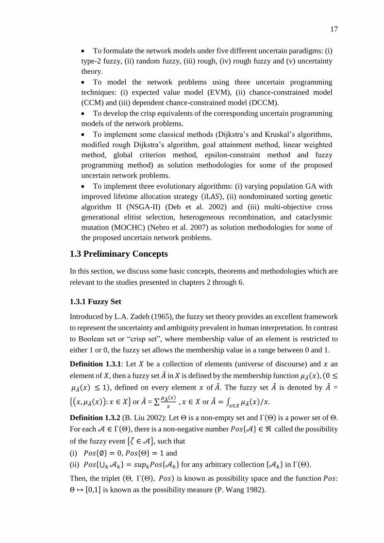
17

To formulate the network models under five different uncertain paradigms: (i)

type-2 fuzzy, (ii) random fuzzy, (iii) rough, (iv) rough fuzzy and (v) uncertainty

theory.

To model the network problems using three uncertain programming

techniques: (i) expected value model (EVM), (ii) chance-constrained model

(CCM) and (iii) dependent chance-constrained model (DCCM).

To develop the crisp equivalents of the corresponding uncertain programming

models of the network problems.

To implement some classical methods (Dijkstra’s and Kruskal’s algorithms,

modified rough Dijkstra’s algorithm, goal attainment method, linear weighted

method, global criterion method, epsilon-constraint method and fuzzy

programming method) as solution methodologies for some of the proposed

uncertain network problems.

To implement three evolutionary algorithms: (i) varying population GA with

improved lifetime allocation strategy (iLAS), (ii) nondominated sorting genetic

algorithm II (NSGA-II) (Deb et al. 2002) and (iii) multi-objective cross

generational elitist selection, heterogeneous recombination, and cataclysmic

mutation (MOCHC) (Nebro et al. 2007) as solution methodologies for some of

the proposed uncertain network problems.

1.3 Preliminary Concepts

In this section, we discuss some basic concepts, theorems and methodologies which are

relevant to the studies presented in chapters 2 through 6.

1.3.1 Fuzzy Set

Introduced by L.A. Zadeh (1965), the fuzzy set theory provides an excellent framework

to represent the uncertainty and ambiguity prevalent in human interpretation. In contrast

to Boolean set or “crisp set”, where membership value of an element is restricted to

either 1 or 0, the fuzzy set allows the membership value in a range between 0 and 1.

Definition 1.3.1: Let 𝑋 be a collection of elements (universe of discourse) and 𝑥 an

element of 𝑋, then a fuzzy set �� in 𝑋 is defined by the membership function 𝜇��(𝑥), (0 ≤

𝜇��(𝑥) ≤ 1), defined on every element 𝑥 of ��. The fuzzy set �� is denoted by �� =

{(𝑥, 𝜇��(𝑥)): 𝑥 ∈ 𝑋} or �� = ∑𝜇��(𝑥)

𝑥 , 𝑥 ∈ 𝑋 or �� = ∫ 𝜇��(𝑥)/𝑥.𝑥∈𝑋

Definition 1.3.2 (B. Liu 2002): Let Θ is a non-empty set and Γ(Θ) is a power set of Θ.

For each 𝒜 ∈ Γ(Θ), there is a non-negative number 𝑃𝑜𝑠{𝒜} ∈ ℜ called the possibility

of the fuzzy event {휁 ∈ 𝒜}, such that

(i) 𝑃𝑜𝑠{∅} = 0, 𝑃𝑜𝑠{Θ} = 1 and

(ii) 𝑃𝑜𝑠{⋃ 𝒜𝑘𝑘 } = 𝑠𝑢𝑝𝑘𝑃𝑜𝑠{𝒜𝑘} for any arbitrary collection {𝒜𝑘} in Γ(Θ).

Then, the triplet (Θ, Γ(Θ), 𝑃𝑜𝑠) is known as possibility space and the function 𝑃𝑜𝑠:

Θ ↦ [0,1] is known as the possibility measure (P. Wang 1982).

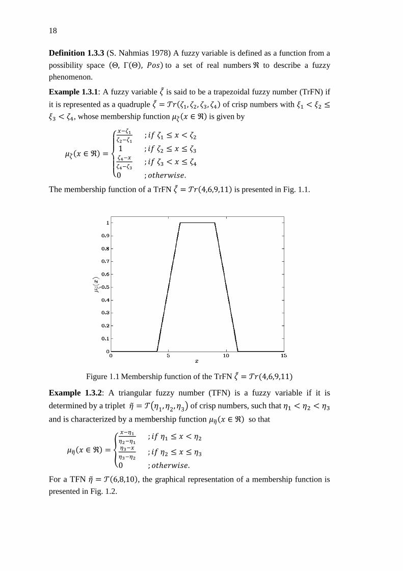
18

Definition 1.3.3 (S. Nahmias 1978) A fuzzy variable is defined as a function from a

possibility space (Θ, Γ(Θ), 𝑃𝑜𝑠) to a set of real numbers ℜ to describe a fuzzy

phenomenon.

Example 1.3.1: A fuzzy variable 휁 is said to be a trapezoidal fuzzy number (TrFN) if

it is represented as a quadruple 휁 = 𝒯𝑟(휁1, 휁2, 휁3, 휁4) of crisp numbers with 𝜉1 < 𝜉2 ≤

𝜉3 < 휁4, whose membership function 𝜇��(𝑥 ∈ ℜ) is given by

𝜇��(𝑥 ∈ ℜ) =

{

𝑥−𝜁1

𝜁2−𝜁1 ; 𝑖𝑓 휁1 ≤ 𝑥 < 휁2

1 ; 𝑖𝑓 휁2 ≤ 𝑥 ≤ 휁3 𝜁4−𝑥

𝜁4−𝜁3 ; 𝑖𝑓 휁3 < 𝑥 ≤ 휁4

0 ; 𝑜𝑡ℎ𝑒𝑟𝑤𝑖𝑠𝑒.

The membership function of a TrFN 휁 = 𝒯𝑟(4,6,9,11) is presented in Fig. 1.1.

= 𝒯𝑟(4,6,9,11)

Example 1.3.2: A triangular fuzzy number (TFN) is a fuzzy variable if it is

determined by a triplet 휂 = 𝒯(휂1, 휂2, 휂3) of crisp numbers, such that 휂1 < 휂2 < 휂3

and is characterized by a membership function 𝜇��(𝑥 ∈ ℜ) so that

𝜇��(𝑥 ∈ ℜ) = {

𝑥−𝜂1

𝜂2−𝜂1 ; 𝑖𝑓 휂1 ≤ 𝑥 < 휂2

𝜂3−𝑥

𝜂3−𝜂2 ; 𝑖𝑓 휂2 ≤ 𝑥 ≤ 휂3


For a TFN 휂 = 𝒯(6,8,10), the graphical representation of a membership function is

presented in Fig. 1.2.

Figure 1.1 Membership function of the TrFN 휁

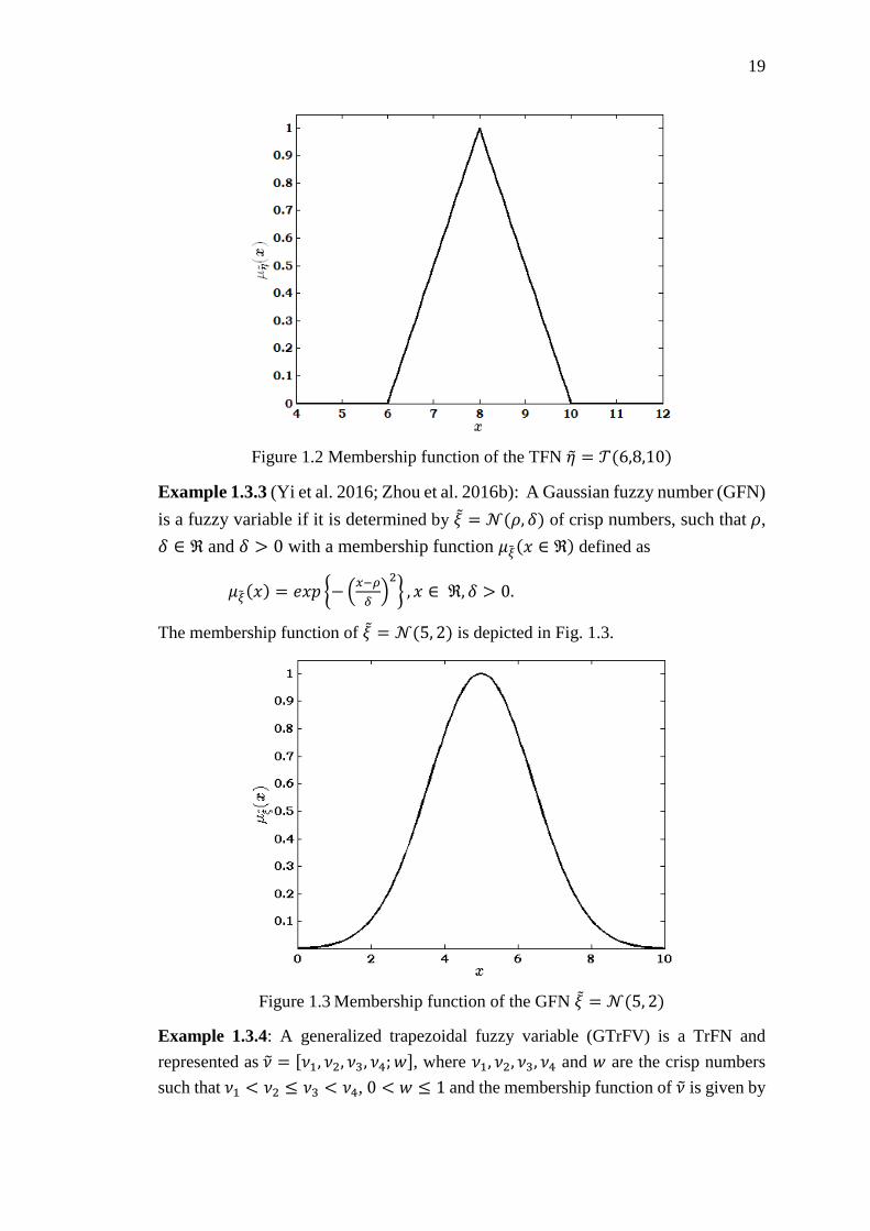
19

Figure 1.2 Membership function of the TFN 휂 = 𝒯(6,8,10)

Example 1.3.3 (Yi et al. 2016; Zhou et al. 2016b): A Gaussian fuzzy number (GFN)

is a fuzzy variable if it is determined by 𝜉 = 𝒩(𝜌, 𝛿) of crisp numbers, such that 𝜌,

𝛿 ∈ ℜ and 𝛿 > 0 with a membership function 𝜇��(𝑥 ∈ ℜ) defined as

𝜇��(𝑥) = 𝑒𝑥𝑝 {− (𝑥−𝜌

𝛿)2

} , 𝑥 ∈ ℜ, 𝛿 > 0.

The membership function of 𝜉 = 𝒩(5, 2) is depicted in Fig. 1.3.

Figure 1.3 Membership function of the GFN 𝜉 = 𝒩(5, 2)

Example 1.3.4: A generalized trapezoidal fuzzy variable (GTrFV) is a TrFN and

represented as 𝜈 = [𝜈1, 𝜈2, 𝜈3, 𝜈4; 𝑤], where 𝜈1, 𝜈2, 𝜈3, 𝜈4 and 𝑤 are the crisp numbers

such that 𝜈1 < 𝜈2 ≤ 𝜈3 < 𝜈4, 0 < 𝑤 ≤ 1 and the membership function of 𝜈 is given by

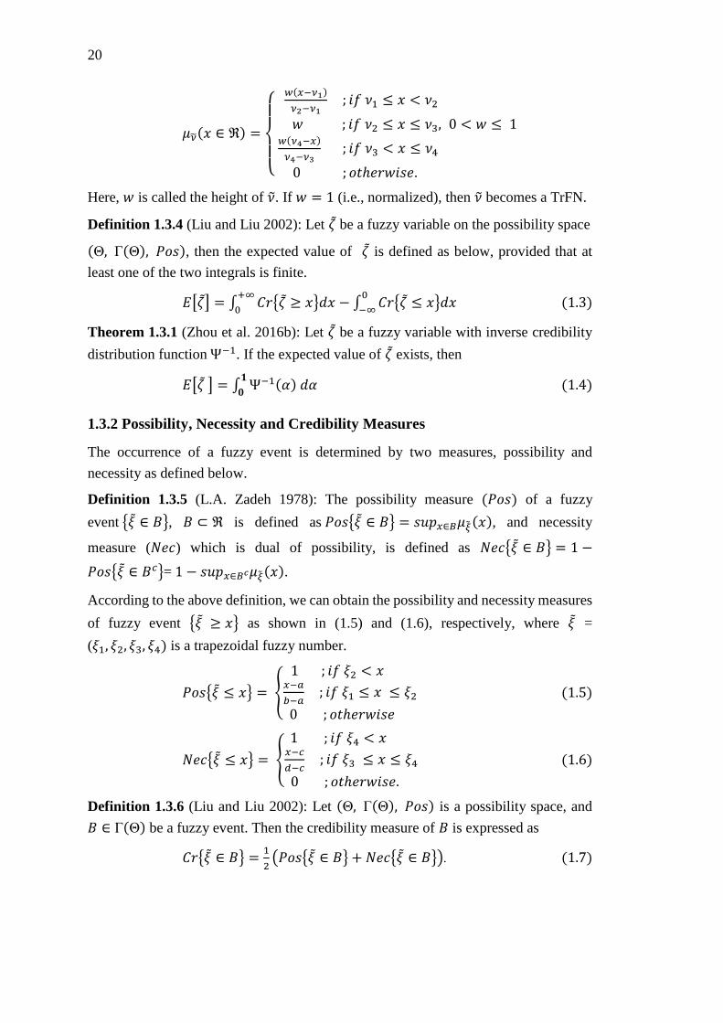
20

𝜇��(𝑥 ∈ ℜ) =

{

𝑤(𝑥−𝜈1)

𝜈2−𝜈1 ; 𝑖𝑓 𝜈1 ≤ 𝑥 < 𝜈2

𝑤 ; 𝑖𝑓 𝜈2 ≤ 𝑥 ≤ 𝜈3, 0 < 𝑤 ≤ 1

𝑤(𝜈4−𝑥)

𝜈4−𝜈3 ; 𝑖𝑓 𝜈3 < 𝑥 ≤ 𝜈4


Here, 𝑤 is called the height of 𝜈. If 𝑤 = 1 (i.e., normalized), then 𝜈 becomes a TrFN.

Definition 1.3.4 (Liu and Liu 2002): Let 휁 be a fuzzy variable on the possibility space

(Θ, Γ(Θ), 𝑃𝑜𝑠), then the expected value of 휁 is defined as below, provided that at

least one of the two integrals is finite.

𝐸[휁] = ∫ 𝐶𝑟{휁 ≥ 𝑥}𝑑𝑥+∞

0− ∫ 𝐶𝑟{휁 ≤ 𝑥}𝑑𝑥

0

−∞ (1.3)

Theorem 1.3.1 (Zhou et al. 2016b): Let 휁 be a fuzzy variable with inverse credibility

distribution function Ψ−1. If the expected value of 휁 exists, then

𝐸[휁 ] = ∫ Ψ−1(𝛼) 𝑑𝛼𝟏

𝟎 (1.4)

1.3.2 Possibility, Necessity and Credibility Measures

The occurrence of a fuzzy event is determined by two measures, possibility and

necessity as defined below.

Definition 1.3.5 (L.A. Zadeh 1978): The possibility measure (𝑃𝑜𝑠) of a fuzzy

event {𝜉 ∈ 𝐵}, 𝐵 ⊂ ℜ is defined as 𝑃𝑜𝑠{𝜉 ∈ 𝐵} = 𝑠𝑢𝑝𝑥∈𝐵𝜇��(𝑥), and necessity

measure (𝑁𝑒𝑐) which is dual of possibility, is defined as 𝑁𝑒𝑐{𝜉 ∈ 𝐵} = 1 −

𝑃𝑜𝑠{𝜉 ∈ 𝐵𝑐}= 1 − 𝑠𝑢𝑝𝑥∈𝐵𝑐𝜇��(𝑥).

According to the above definition, we can obtain the possibility and necessity measures

of fuzzy event {𝜉 ≥ 𝑥} as shown in (1.5) and (1.6), respectively, where 𝜉 =

(𝜉1, 𝜉2, 𝜉3, 𝜉4) is a trapezoidal fuzzy number.

𝑃𝑜𝑠{𝜉 ≤ 𝑥} = {

1 ; 𝑖𝑓 𝜉2 < 𝑥 𝑥−𝑎

𝑏−𝑎 ; 𝑖𝑓 𝜉1 ≤ 𝑥 ≤ 𝜉2

0 ; 𝑜𝑡ℎ𝑒𝑟𝑤𝑖𝑠𝑒

(1.5)

𝑁𝑒𝑐{𝜉 ≤ 𝑥} = {

1 ; 𝑖𝑓 𝜉4 < 𝑥 𝑥−𝑐

𝑑−𝑐 ; 𝑖𝑓 𝜉3 ≤ 𝑥 ≤ 𝜉4


(1.6)

Definition 1.3.6 (Liu and Liu 2002): Let (Θ, Γ(Θ), 𝑃𝑜𝑠) is a possibility space, and

𝐵 ∈ Γ(Θ) be a fuzzy event. Then the credibility measure of 𝐵 is expressed as

𝐶𝑟{𝜉 ∈ 𝐵} =1

2(𝑃𝑜𝑠{𝜉 ∈ 𝐵} + 𝑁𝑒𝑐{𝜉 ∈ 𝐵}). (1.7)

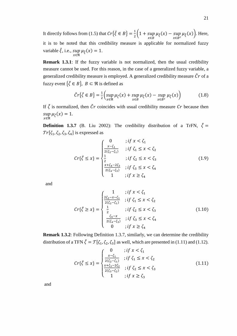
21

It directly follows from (1.5) that 𝐶𝑟{𝜉 ∈ 𝐵} =1

2(1 + 𝑠𝑢𝑝

𝑥∈𝐵𝜇��(𝑥) − 𝑠𝑢𝑝

𝑥∈𝐵𝑐𝜇��(𝑥)). Here,

it is to be noted that this credibility measure is applicable for normalized fuzzy

variable 𝜉, i.e., 𝑠𝑢𝑝𝑥∈ℜ

𝜇��(𝑥) = 1.

Remark 1.3.1: If the fuzzy variable is not normalized, then the usual credibility

measure cannot be used. For this reason, in the case of a generalized fuzzy variable, a

generalized credibility measure is employed. A generalized credibility measure ��𝑟 of a

fuzzy event {휁 ∈ 𝐵}, 𝐵 ⊂ ℜ is defined as

��𝑟{휁 ∈ 𝐵} =1

2(𝑠𝑢𝑝𝑥∈ℜ

𝜇��(𝑥) + 𝑠𝑢𝑝𝑥∈𝐵

𝜇��(𝑥) − 𝑠𝑢𝑝𝑥∈𝐵𝑐

𝜇��(𝑥)) (1.8)

If 휁 is normalized, then ��𝑟 coincides with usual credibility measure 𝐶𝑟 because then

𝑠𝑢𝑝𝑥∈ℜ

𝜇��(𝑥) = 1.

Definition 1.3.7 (B. Liu 2002): The credibility distribution of a TrFN, 휁 =

𝒯𝑟[휁1, 휁2, 휁3, 휁4] is expressed as

𝐶𝑟{휁 ≤ 𝑥} =

{

0 ; 𝑖𝑓 𝑥 < 휁1 𝑥−𝜁1

2(𝜁2−𝜁1) ; 𝑖𝑓 휁1 ≤ 𝑥 < 휁2

1

2 ; 𝑖𝑓 휁2 ≤ 𝑥 < 휁3𝑥+𝜁4−2𝜁3

2(𝜁4−𝜁3) ; 𝑖𝑓 휁3 ≤ 𝑥 < 휁4

1 ; 𝑖𝑓 𝑥 ≥ 휁4

(1.9)

and

𝐶𝑟{휁 ≥ 𝑥} =

{

1 ; 𝑖𝑓 𝑥 < 휁1 2𝜁2−𝑥−𝜁1

2(𝜁2−𝜁1) ; 𝑖𝑓 휁1 ≤ 𝑥 < 휁2

1

2 ; 𝑖𝑓 휁2 ≤ 𝑥 < 휁3𝜁4−𝑥

2(𝜁4−𝜁3) ; 𝑖𝑓 휁3 ≤ 𝑥 < 휁4

0 ; 𝑖𝑓 𝑥 ≥ 휁4

(1.10)

Remark 1.3.2: Following Definition 1.3.7, similarly, we can determine the credibility

distribution of a TFN 휁 = 𝒯[휁1, 휁2, 휁3] as well, which are presented in (1.11) and (1.12).

𝐶𝑟{휁 ≤ 𝑥} =

{

0 ; 𝑖𝑓 𝑥 < 휁1 𝑥−𝜁1

2(𝜁2−𝜁1) ; 𝑖𝑓 휁1 ≤ 𝑥 < 휁2

𝑥+𝜁3−2𝜁2

2(𝜁3−𝜁2) ; 𝑖𝑓 휁2 ≤ 𝑥 < 휁3

1 ; 𝑖𝑓 𝑥 ≥ 휁3

(1.11)

and

22

𝐶𝑟{휁 ≥ 𝑥} =

{

1 ; 𝑖𝑓 𝑥 < 휁1 2𝜁2−𝜁1−𝑥

2(𝜁2−𝜁1) ; 𝑖𝑓 휁1 ≤ 𝑥 < 휁2

𝜁3−𝑥

2(𝜁3−𝜁2) ; 𝑖𝑓 휁2 ≤ 𝑥 < 휁3

0 ; 𝑖𝑓 𝑥 ≥ 휁3

(1.12)

Theorem 1.3.2 (Gao and Lu 2005): Let 휁 = 𝒯𝑟[휁1, 휁2, 휁3, 휁4] is a TrFN and 𝛼 is the

predetermined confidence level, then

(i) while 𝛼 ∈ (0,0.5], 𝐶𝑟{𝜉 ≤ 𝑥 } ≥ 𝛼 if and only if 𝑥 ≥ (1 − 2𝛼)𝜉1 + 2𝛼𝜉2

(ii) while 𝛼 ∈ (0.5,1], 𝐶𝑟{𝜉 ≤ 𝑥 } ≥ 𝛼 if and only if 𝑥 ≥ (2 − 2𝛼)𝜉3 + (2𝛼 − 1)𝜉4.

Remark 1.3.3: If 휁 = 𝒯[휁1, 휁2, 휁3] is a TFN with a predetermined confidence level 𝛼,

then

(i) while 𝛼 ∈ (0,0.5], 𝐶𝑟{𝜉 ≤ 𝑥 } ≥ 𝛼 if and only if 𝑥 ≥ (1 − 2𝛼)𝜉1 + 2𝛼𝜉2

(ii) while 𝛼 ∈ (0.5,1], 𝐶𝑟{𝜉 ≤ 𝑥 } ≥ 𝛼 if and only if 𝑥 ≥ (2 − 2𝛼)𝜉2 + (2𝛼 − 1)𝜉3.

Lemma 1.3.1: Let 휁 = 𝒯𝑟[휁1, 휁2, 휁3, 휁4] be a TrFN and 𝛼(∈ [0,1]) is the given

confidence level, then

(i) if 𝛼 ≤1

2, then 𝐶𝑟{휁 ≥ 𝑥} ≥ 𝛼 if and only if, (1 − 2 𝛼)휁4 + 2𝛼휁3 ≥ 𝑥

(ii) if 𝛼 >1

2, then 𝐶𝑟{휁 ≥ 𝑥} ≥ 𝛼 if and only if, (2 − 2 𝛼)휁2 + (2𝛼 − 1)휁1 ≥ 𝑥.

Proof:

(i) When 𝛼 ≤1

2 and 𝐶𝑟{휁 ≥ 𝑥} ≥ 𝛼, then we have either 휁3 ≤ 𝑥 < 휁4 or {

𝜁4−𝑥

2(𝜁4−𝜁3)} ≥

𝛼. Considering, {𝜁4−𝑥

2(𝜁4−𝜁3)} ≥ 𝛼 ⇔ (1 − 2 𝛼)휁4 + 2𝛼휁3 ≥ 𝑥. Again, (1 − 2 𝛼)휁4 +

2𝛼휁3 ≥ 𝑥 holds good for 휁2 ≤ 𝑥 < 휁3 since 𝛼 ≤1

2. Conversely, when 휁3 ≤ 𝑥, then

𝐶𝑟{휁 ≥ 𝑥} ≥ 𝛼 if 𝐶𝑟{휁 ≥ 𝑥} is at least 1

2. Therefore, (1 − 2 𝛼)휁4 + 2𝛼휁3 ≥ 𝑥 ⇔

{𝜁4−𝑥

2(𝜁4−𝜁3)} ≥ 𝛼 ⇔ 𝐶𝑟{휁 ≥ 𝑥} ≥ 𝛼.

(ii) When 𝛼 >1

2 and 𝐶𝑟{휁 ≥ 𝑥} ≥ 𝛼, then we observe that either 𝑥 ≤ 휁1 or {

2𝜁2−𝑥−𝜁1

2(𝜁2−𝜁1)} ≥

𝛼. Considering, each of the observed cases, we have (2 − 2 𝛼)휁2 + (2𝛼 − 1)휁1 ≥ 𝑥.

Conversely, when 𝑥 < 휁1then 𝐶𝑟{휁 ≥ 𝑥} = 1 ≥ 𝛼. Now (2 − 2 𝛼)휁2 + (2𝛼 − 1)휁1 ≥

𝑥 ⇔ {2𝜁2−𝑥−𝜁1

2(𝜁2−𝜁1)} ≥ 𝛼, which eventually means 𝐶𝑟{휁 ≥ 𝑥} ≥ 𝛼.

Definition 1.3.8 (Zhou et al. 2016b): The credibility distribution of a GFN 휁 = 𝒩(ρ, 𝛿)

is represented as

𝐶𝑟{휁 ≤ 𝑥} = {

1

2𝑒𝑥𝑝 {−(

𝜌−𝑥

𝛿)2

} ; 𝑖𝑓 𝑥 ≤ 𝜌

1 −1

2𝑒𝑥𝑝 {− (

𝑥−𝜌

𝛿)2

} ; 𝑖𝑓 𝑥 > 𝜌 (1.13)

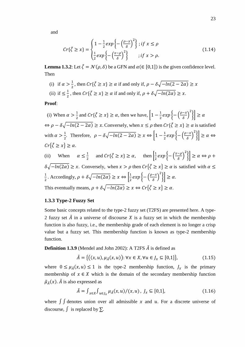
23

and

𝐶𝑟{휁 ≥ 𝑥} = {1 −

1

2𝑒𝑥𝑝 {− (

𝜌−𝑥

𝛿)2

} ; 𝑖𝑓 𝑥 ≤ 𝜌

1

2𝑒𝑥𝑝 {−(

𝑥−𝜌

𝛿)2

} ; 𝑖𝑓 𝑥 > 𝜌. (1.14)

Lemma 1.3.2: Let 휁 = 𝒩(𝜌, 𝛿) be a GFN and 𝛼(∈ [0,1]) is the given confidence level.

Then

(i) if 𝛼 >1

2 , then 𝐶𝑟{휁 ≥ 𝑥} ≥ 𝛼 if and only if, 𝜌 − 𝛿√−𝑙𝑛(2 − 2𝛼) ≥ 𝑥

(ii) if ≤1

2 , then 𝐶𝑟{휁 ≥ 𝑥} ≥ 𝛼 if and only if, 𝜌 + 𝛿√−𝑙𝑛(2𝛼) ≥ 𝑥.

Proof:

(i) When 𝛼 >1

2 and 𝐶𝑟{휁 ≥ 𝑥} ≥ 𝛼, then we have, [1 −

1

2𝑒𝑥𝑝 {−(

𝜌−𝑥

𝛿)2

}] ≥ 𝛼

⇔ 𝜌 − 𝛿√−𝑙𝑛(2 − 2𝛼) ≥ 𝑥. Conversely, when 𝑥 ≤ 𝜌 then 𝐶𝑟{휁 ≥ 𝑥} ≥ 𝛼 is satisfied

with 𝛼 >1

2. Therefore, 𝜌 − 𝛿√−𝑙𝑛(2 − 2𝛼) ≥ 𝑥 ⇔ [1 −

1

2𝑒𝑥𝑝 {−(

𝜌−𝑥

𝛿)2

}] ≥ 𝛼 ⇔

𝐶𝑟{휁 ≥ 𝑥} ≥ 𝛼.

(ii) When 𝛼 ≤1

2 and 𝐶𝑟{휁 ≥ 𝑥} ≥ 𝛼, then [

1

2𝑒𝑥𝑝 {−(

𝑥−𝜌

𝛿)2

}] ≥ 𝛼 ⇔ 𝜌 +

𝛿√−𝑙𝑛(2𝛼) ≥ 𝑥. Conversely, when 𝑥 > 𝜌 then 𝐶𝑟{휁 ≥ 𝑥} ≥ 𝛼 is satisfied with 𝛼 ≤

1

2 . Accordingly, 𝜌 + 𝛿√−𝑙𝑛(2𝛼) ≥ 𝑥 ⇔ [

1

2𝑒𝑥𝑝 {−(

𝜌−𝑥

𝛿)2

}] ≥ 𝛼.

This eventually means, 𝜌 + 𝛿√−𝑙𝑛(2𝛼) ≥ 𝑥 ⇔ 𝐶𝑟{휁 ≥ 𝑥} ≥ 𝛼.

1.3.3 Type-2 Fuzzy Set

Some basic concepts related to the type-2 fuzzy set (T2FS) are presented here. A type-

2 fuzzy set �� in a universe of discourse 𝑋 is a fuzzy set in which the membership

function is also fuzzy, i.e., the membership grade of each element is no longer a crisp

value but a fuzzy set. This membership function is known as type-2 membership

function.

Definition 1.3.9 (Mendel and John 2002): A T2FS �� is defined as

�� = {((𝑥, 𝑢), 𝜇��(𝑥, 𝑢)): ∀𝑥 ∈ 𝑋, ∀𝑢 ∈ 𝐽𝑥 ⊆ [0,1]}, (1.15)

where 0 ≤ 𝜇��(𝑥, 𝑢) ≤ 1 is the type-2 membership function, 𝐽𝑥 is the primary

membership of 𝑥 ∈ 𝑋 which is the domain of the secondary membership function

𝜇��(𝑥). �� is also expressed as

�� = ∫𝑥∈𝑋

∫𝑢∈𝐽𝑥

𝜇��(𝑥, 𝑢) (𝑥, 𝑢)⁄ , 𝐽𝑥 ⊆ [0,1], (1.16)

where ∫ ∫ denotes union over all admissible 𝑥 and 𝑢. For a discrete universe of

discourse, ∫ is replaced by ∑.

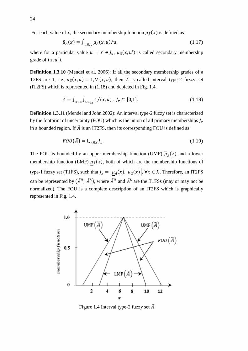
24

For each value of 𝑥, the secondary membership function 𝜇��(𝑥) is defined as

𝜇��(𝑥) = ∫𝑢∈𝐽𝑥𝜇��(𝑥, 𝑢) 𝑢⁄ , (1.17)

where for a particular value 𝑢 = 𝑢′ ∈ 𝐽𝑥, 𝜇��(𝑥, 𝑢′) is called secondary membership

grade of (𝑥, 𝑢′).

Definition 1.3.10 (Mendel et al. 2006): If all the secondary membership grades of a

T2FS are 1, i.e., 𝜇��(𝑥, 𝑢) = 1, ∀ (𝑥, 𝑢), then �� is called interval type-2 fuzzy set

(IT2FS) which is represented in (1.18) and depicted in Fig. 1.4.

�� = ∫𝑥∈𝑋

∫𝑢∈𝐽𝑥

1 (𝑥, 𝑢)⁄ , 𝐽𝑥 ⊆ [0,1]. (1.18)

Definition 1.3.11 (Mendel and John 2002): An interval type-2 fuzzy set is characterized

by the footprint of uncertainty (FOU) which is the union of all primary memberships 𝐽𝑥

in a bounded region. If �� is an IT2FS, then its corresponding FOU is defined as

𝐹𝑂𝑈(��) = ⋃ 𝐽𝑥𝑥∈𝑋 . (1.19)

The FOU is bounded by an upper membership function (UMF) 𝜇��(𝑥) and a lower

membership function (LMF) 𝜇��(𝑥), both of which are the membership functions of

type-1 fuzzy set (T1FS), such that 𝐽𝑥 = [𝜇��(𝑥), 𝜇��(𝑥)], ∀𝑥 ∈ 𝑋. Therefore, an IT2FS

can be represented by (��𝑈, ��𝐿), where ��𝑈 and ��𝐿 are the T1FSs (may or may not be

normalized). The FOU is a complete description of an IT2FS which is graphically

represented in Fig. 1.4.

Figure 1.4 Interval type-2 fuzzy set ��

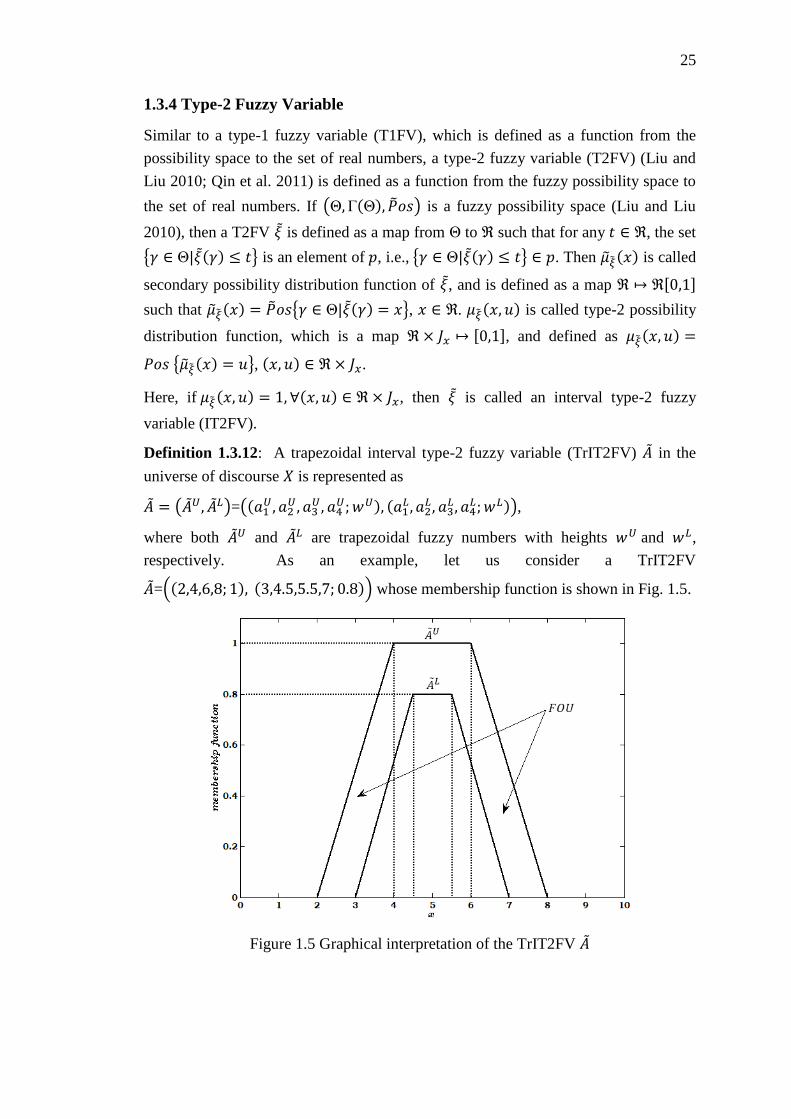
25

1.3.4 Type-2 Fuzzy Variable

Similar to a type-1 fuzzy variable (T1FV), which is defined as a function from the

possibility space to the set of real numbers, a type-2 fuzzy variable (T2FV) (Liu and

Liu 2010; Qin et al. 2011) is defined as a function from the fuzzy possibility space to

the set of real numbers. If (Θ,Γ(Θ), ��𝑜𝑠) is a fuzzy possibility space (Liu and Liu

2010), then a T2FV 𝜉 is defined as a map from Θ to ℜ such that for any 𝑡 ∈ ℜ, the set

{𝛾 ∈ Θ|𝜉(𝛾) ≤ 𝑡} is an element of 𝑝, i.e., {𝛾 ∈ Θ|𝜉(𝛾) ≤ 𝑡} ∈ 𝑝. Then 𝜇��(𝑥) is called

secondary possibility distribution function of 𝜉, and is defined as a map ℜ ↦ ℜ[0,1]

such that 𝜇��(𝑥) = ��𝑜𝑠{𝛾 ∈ Θ|𝜉(𝛾) = 𝑥}, 𝑥 ∈ ℜ. 𝜇��(𝑥, 𝑢) is called type-2 possibility

distribution function, which is a map ℜ × 𝐽𝑥 ↦ [0,1], and defined as 𝜇��(𝑥, 𝑢) =

𝑃𝑜𝑠 {��(𝑥) = 𝑢}, (𝑥, 𝑢) ∈ ℜ × 𝐽𝑥.

Here, if 𝜇��(𝑥, 𝑢) = 1, ∀(𝑥, 𝑢) ∈ ℜ × 𝐽𝑥, then 𝜉 is called an interval type-2 fuzzy

variable (IT2FV).

Definition 1.3.12: A trapezoidal interval type-2 fuzzy variable (TrIT2FV) �� in the

universe of discourse 𝑋 is represented as

�� = (��𝑈, ��𝐿)=((𝑎1𝑈, 𝑎2

𝑈, 𝑎3𝑈, 𝑎4

𝑈; 𝑤𝑈), (𝑎1𝐿 , 𝑎2

𝐿 , 𝑎3𝐿 , 𝑎4

𝐿; 𝑤𝐿)),

where both ��𝑈 and ��𝐿 are trapezoidal fuzzy numbers with heights 𝑤𝑈 and 𝑤𝐿,

respectively. As an example, let us consider a TrIT2FV

��=((2,4,6,8; 1), (3,4.5,5.5,7; 0.8)) whose membership function is shown in Fig. 1.5.

Figure 1.5 Graphical interpretation of the TrIT2FV ��

26

1.3.5 Random Fuzzy Variable

B. Liu (2001) introduced the concept of a random fuzzy variable, which is a fuzzy

variable on the universal set of random variables. In this section, we present some

definitions related to the random fuzzy variable.

Definition 1.3.13 (B. Liu 2001, 2002): A random fuzzy variable is a function from

possibility space (Θ, Γ(Θ), 𝑃𝑜𝑠) to a set of random variables ℛ.

Definition 1.3.14 (B. Liu 2001, 2002): Let 휁𝑖 be random fuzzy variables defined on the

possibility spaces (Θ𝑖, Γ(Θ𝑖), 𝑃𝑜𝑠𝑖), 𝑖 = 1,2,3… , 𝑛, respectively, and 𝑓: ℜ𝑛 ↦ ℜ a

measurable function. Then, 휁 = (휁1, 휁2, … , 휁𝑛) is a random fuzzy variable on the

product possibility space (Θ, Γ(Θ), 𝑃𝑜𝑠), defined as

휁(휃1, 휃2, … , 휃𝑛) = 𝑓 (휁1(휃1), 휁2(휃2), … , 휁𝑛(휃𝑛)) (1.20)

for all (휃1, 휃2, … , 휃𝑛) ∈ Θ.

Definition 1.3.15 (B. Liu 2002; Liu and Liu 2003): Let 휁 be a random fuzzy variable

defined on the possibility space (Θ, Γ(Θ), 𝑃𝑜𝑠). Then the expected value 𝐸 [휁] of 휁 is

defined by

𝐸 [휁] = ∫ 𝐶𝑟 {휃 ∈ Θ|𝐸 [휁(휃)] ≥ 𝑥} 𝑑𝑥 − ∫ 𝐶𝑟 {휃 ∈ Θ|𝐸 [휁(휃)] ≤ 𝑥} 𝑑𝑥0

−∞

+∞

0 (1.21)

provided that one of the two integrals is finite.

Remark 1.3.4 (B. Liu 2002): If the random fuzzy variable 휁 degenerates to a random

variable, then the expected value operator becomes

𝐸 [휁] = ∫ 𝑃𝑟 {휁 ≥ 𝑥} 𝑑𝑥 − ∫ 𝑃𝑟 {휁 ≤ 𝑥} 𝑑𝑥0

−∞

+∞

0. (1.22)

Remark 1.3.5 (B. Liu 2002): If the random fuzzy variable 휁 degenerates to a fuzzy

variable, then the expected value operator becomes

𝐸 [휁] = ∫ 𝐶𝑟 {휁 ≥ 𝑥} 𝑑𝑥 − ∫ 𝐶𝑟 {휁 ≤ 𝑥} 𝑑𝑥0

−∞

+∞

0. (1.23)

Definition 1.3.16 (B. Liu 2001, 2002): Let 휁 = (휁1, 휁2, … , 휁𝑛) be a random fuzzy vector

on the possibility space (Θ, Γ(Θ), 𝑃𝑜𝑠), and 𝑓𝑝: ℜ𝑛 ↦ ℜ be continuous

functions, 𝑝 = 1,2, … , 𝑘. Then the primitive chance at predetermined confidence labels

𝛼 and 𝛽, for a random fuzzy event characterized by 𝑓𝑝 (휁) ≤ 0, 𝑝 = 1,2, … , 𝑘 is a

function from [0,1] to [0,1] and is defined below in (1.24).

27

𝐶ℎ {𝑓𝑝 (휁) ≤ 0, 𝑝 = 1,2, … , 𝑘} (𝛼)=𝑠𝑢𝑝 {𝛽|𝑃𝑜𝑠 {휃 ∈ 𝛩| 𝑃𝑟 {𝑓𝑝(��(𝜃))≤0

𝑝=1,2,…,𝑘} ≥ 𝛽} ≥ 𝛼}

(1.24)

Remark 1.3.6: In this thesis, the random fuzzy chance-constrained programming

model has been developed using the definition of the primitive chance as defined in

(1.25), where a random fuzzy event is measured with a credibility measure and a

probability measure, which are represented as 𝐶𝑟 and 𝑃𝑟, respectively.

𝐶ℎ {𝑓𝑝 (휁) ≤ 0, 𝑝 = 1,2, … , 𝑘} (𝛼)=𝑠𝑢𝑝 {𝛽|𝐶𝑟 {휃 ∈ 𝛩| 𝑃𝑟 {𝑓𝑝(��(𝜃))≤0

𝑝=1,2,…,𝑘} ≥ 𝛽} ≥ 𝛼}

(1.25)

1.3.6 Rough Set

Rough set theory, introduced by Z. Pawlak (1982), is a mathematical approach to model

imperfect knowledge. The rudimentary conjecture in rough set theory is to recognize

every object in the universe on the basis of information (data, knowledge). Rough set

models vagueness in a different way altogether. Unlike fuzzy set, rough set expresses

the vagueness in terms of boundary region of a set. A rough set is represented by using

two approximation sets, the lower approximation set and the upper approximation set.

Let 𝑋 be the universe of discourse of non-empty finite set of objects and 𝐴 be the non-

empty finite set of attributes, then the pair 𝑆 = (𝑋, 𝐴) is said to be an information

system. For any 𝐵 ⊆ 𝐴, there exists an indiscernibility (similarity) relation 𝑅(𝐵) such

that 𝑅(𝐵) = {(𝑥, 𝑦) ∈ 𝑋 × 𝑋| ∀𝑎 ∈ 𝐵, 𝑎(𝑥) = 𝑎(𝑦)}, where 𝑎(𝑥) denote the value of

an attribute 𝑎 for the element 𝑥. 𝑅(𝐵) is called the 𝐵-indiscernibility relation having

equivalence classes [𝑥]𝑅. We define the lower approximation and the upper

approximation of the set 𝑋 in order to classify the elements of set 𝑋.

An information system 𝑆 = (𝑋, 𝐴), 𝐵 ⊆ 𝐴, 𝑇 ⊆ 𝑋 can be approximated based on the

information of 𝐵 into 𝐵-lower approximation and 𝐵-upper approximation (Z. Pawlak

1982) of 𝑇, which are defined as

𝐵(𝑇) = {𝑥|[𝑥]𝐵 ⊆ 𝑇}

and

𝐵(𝑇) = {𝑥|[𝑥]𝐵: [𝑥]𝐵⋂𝑇 ≠ ∅}.

Note that the objects in 𝐵(𝑇) become the certain members of 𝑇, whereas objects in

𝐵(𝑇) become the possible members of 𝑇. The 𝐵 −boundary region of 𝑇 is defined as

𝐵𝑁𝐵(𝑇) = 𝐵(𝑇) − 𝐵(𝑇).

Fig. 1.6 depicts a schematic representation of a rough set 𝑆, which is defined on

equivalence classes. The equivalence classes are determined by the small squares in the

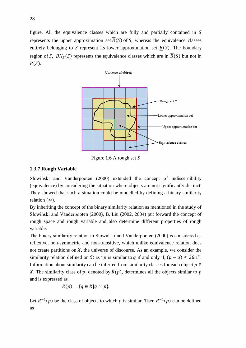
28

figure. All the equivalence classes which are fully and partially contained in 𝑆

represents the upper approximation set 𝐵(𝑆) of 𝑆, whereas the equivalence classes

entirely belonging to 𝑆 represent its lower approximation set 𝐵(𝑆). The boundary

region of 𝑆, 𝐵𝑁𝐵(𝑆) represents the equivalence classes which are in 𝐵(𝑆) but not in

𝐵(𝑆).

Figure 1.6 A rough set 𝑆

1.3.7 Rough Variable

Słowiński and Vanderpooten (2000) extended the concept of indiscernibility

(equivalence) by considering the situation where objects are not significantly distinct.

They showed that such a situation could be modelled by defining a binary similarity

relation (≃).

By inheriting the concept of the binary similarity relation as mentioned in the study of

Słowiński and Vanderpooten (2000), B. Liu (2002, 2004) put forward the concept of

rough space and rough variable and also determine different properties of rough

variable.

The binary similarity relation in Słowiński and Vanderpooten (2000) is considered as

reflexive, non-symmetric and non-transitive, which unlike equivalence relation does

not create partitions on 𝑋, the universe of discourse. As an example, we consider the

similarity relation defined on ℜ as “𝑝 is similar to 𝑞 if and only if, (𝑝 − 𝑞) ≤ 26.1”.

Information about similarity can be inferred from similarity classes for each object 𝑝 ∈

𝑋. The similarity class of 𝑝, denoted by 𝑅(𝑝), determines all the objects similar to 𝑝

and is expressed as

𝑅(𝑝) = {𝑞 ∈ 𝑋|𝑞 ≃ 𝑝}.

Let 𝑅−1(𝑝) be the class of objects to which 𝑝 is similar. Then 𝑅−1(𝑝) can be defined

as

29

𝑅−1(𝑝) = {𝑞 ∈ 𝑋| 𝑝 ≃ 𝑞}.

The lower and upper approximations of the set based on binary similarity relation 𝑅,

proposed by Słowiński and Vanderpooten (2000), are defined as follows.

Definition 1.3.17 (Słowiński and Vanderpooten 2000): Considering 𝑈 ⊆ 𝑋 and a

binary similarity relation 𝑅 defined on 𝑋, the lower approximation of 𝑈, denoted by 𝑈,

is defined as

𝑈 = {𝑥 ∈ 𝑋|𝑅−1(𝑥) ⊆ 𝑈},

while the upper approximation of 𝑈, denoted by 𝑈, is defined as

𝑈 = ⋃ 𝑅(𝑥)𝑥∈𝑈 .

Thus, the lower approximation is a subset containing the objects which surely belong

to the set 𝑈, whereas the upper approximation is a superset containing the objects which

possibly belong to 𝑈.

Theorem 1.3.3 (Słowiński and Vanderpooten 2000): Consider a subset 𝑈 ⊆ 𝑋 and a

binary similarity relation 𝑅 defined on 𝑋, then, 𝑈 ⊆ 𝑈 ⊆ 𝑈.

Example 1.3.5: We consider a set of products which are sequentially arranged in

decreasing order of their respective prices. We define the similarity relation ≃ on ℜ,

such that the cost of product 𝑝 ≃ cost of product 𝑞 if and only if 𝑐(𝑝) − 𝑐(𝑞) ≤ $10,

where 𝑐(⋅) is the manufacturing cost of a product. The cost of a product may vary over

a time interval due to the fluctuation in cost of raw materials and transportation costs.

The existence of such factors directly influences the fluctuation of the manufacturing

cost of the product. In order to capture such fluctuation, 𝑐(⋅) can be represented by

intervals. If the cost of the product is around $80 which is estimated by an expert as the

set [60, 90], then the corresponding lower and upper approximations with respect to

‘≃’ are [60, 90] = [70, 80] and [60, 90] = [50, 100], respectively.

B. Liu (2004) defined some axioms and certain definitions, which are stated below,

while introducing the concept of rough variable.

Let Ʌ be a non-empty set, 𝒜 be a 𝜎-algebra of subsets of Ʌ, ∆ be an element in 𝒜 and

𝜌 be the non-negative real-valued additive set function on 𝒜, then the axioms are as

follows.

Axiom 1: 𝜌{Ʌ} < +∞

Axiom 2: 𝜌{∆ } > 0

Axiom 3: 𝜌{A} ≥ 0 for any A ∈ 𝒜

Axiom 4: For every countable sequence of mutually disjoint events {A𝑖}𝑖=1∞ , we have,

𝜌{⋃ A𝑖∞𝑖=1 } = ∑ 𝜌{A𝑖}

∞𝑖=1 .

Definition 1.3.18 (B. Liu 2002): Let Ʌ be a non-empty set, 𝒜 a 𝜎-algebra of subsets of

Ʌ, ∆ be an element in 𝒜 and 𝜌 be the non-negative real-valued additive set function on

30

𝒜 satisfying Axiom 1 through Axiom 4. Then the quadruple (Ʌ, ∆,𝒜, 𝜌) is called a

rough space.

Definition 1.3.19 (B. Liu 2002): A rough variable 𝜉 on a rough space (Ʌ, ∆,𝒜, 𝜌) is a

measurable function from Ʌ to the set of real numbers ℜ such that for every Borel

set ℬ of ℜ we have, { ∈ Ʌ|휁() ∈ ℬ} ∈ 𝒜. Then the lower and upper approximations

of the rough variable 휁 are represented as follow.

휁 = {휁()| ∈ ∆}

and

휁 = {휁()| ∈ Ʌ}

Since ∆ ⊂ Ʌ, it becomes obvious that 휁 ⊂ 휁. The extreme cases for ∆ are ∆ =

∅ and ∆ = Ʌ. If ∆ = ∅, then 휁 will be a null set. If ∆ = Ʌ, then 휁 = 휁, and 휁 becomes

an ordinary set.

Example 1.3.6: Let Ʌ = {𝑥|0 ≤ 𝑥 ≤ 80} and ∆= {𝑥|20 ≤ 𝑥 ≤ 50}, then the function,

휁(𝑥) = 𝑥|(𝑥 𝑚𝑜𝑑 6) = 0 is a rough variable defined on (Ʌ, ∆,𝒜, 𝜌).

Example 1.3.7: Let us consider a rough variable 휁 = ([𝑎, 𝑏], [𝑐, 𝑑]), c ≤ 𝑎 ≤ 𝑏 ≤ 𝑑,

defined on the rough space (Ʌ, ∆,𝒜, 𝜌), where [𝑎, 𝑏] and [𝑐, 𝑑] are lower and upper

approximations of 휁, respectively. This eventually means that the representing elements

of [𝑎, 𝑏] are certainly the members of 휁 and that belonging to [𝑐, 𝑑] are the possible

members of 휁. Here Ʌ = {𝑥|𝑐 ≤ 𝑥 ≤ 𝑑}, ∆= {𝑥|𝑎 ≤ 𝑥 ≤ 𝑏} and 휁(𝑥) = 𝑥, ∀𝑥 ∈ Ʌ. 𝒜

is the 𝜎-algebra on Ʌ and 𝜌 is the Lebesgue measure.

1.3.8 Trust Measure of Rough Variable

Definition 1.3.20 (B. Liu 2002): Let 휁 be a rough vector on a rough space (Ʌ,

∆,𝒜, 𝜌) and 𝜏𝑘: ℜ𝑛 → ℜ be the continuous function, 𝑘 = 1,2, … ,𝑚. Then the upper

trust measure and the lower trust measure of the rough event, represented by 𝜏𝑘(휁) ≤

0, 𝑘 = 1,2, … ,𝑚, are defined as follows.

𝑇𝑟{𝜏𝑘(ζ) ≤ 0, 𝑘 = 1,2, … ,𝑚} =𝜌{ ∈ Ʌ|𝜏𝑘(ζ()) ≤ 0, 𝑘 = 1,2, … ,𝑚}

𝜌{Ʌ}.

(1.26)

𝑇𝑟{𝜏𝑘(ζ) ≤ 0, 𝑘 = 1,2, … ,𝑚} =𝜌{ ∈ ∆|𝜏𝑘(ζ()) ≤ 0, 𝑘 = 1,2, … ,𝑚}

𝜌{∆}.

(1.27)

If 𝜌(∆) = 0, then 𝑇𝑟{𝜏𝑘(휁) ≤ 0, 𝑘 = 1,2, … , 𝑚} ≡ 𝑇𝑟{𝜏𝑘(ζ) ≤ 0, 𝑘 = 1,2, … ,𝑚}.

The trust measure of a rough event is defined as the mean of lower and upper trusts as

given below.

31

𝑇𝑟{𝜏𝑘(ζ) ≤ 0, 𝑘 = 1,2, … ,𝑚}

=(𝑇𝑟{𝜏𝑘(ζ) ≤ 0, 𝑘 = 1,2, … ,𝑚} + 𝑇𝑟{𝜏𝑘(ζ) ≤ 0, 𝑘 = 1,2, … ,𝑚})

2.

(1.28)

Remark 1.3.7 (B. Liu 2002): The value of upper trust, lower trust and trust of a rough

event, characterized by { 𝜏𝑘(휁) ≤ 0, 𝑘 = 1,2, … ,𝑚}, are within [0,1]. A rough event

must hold if its trust is 1 and it fails when its trust is 0.

For a given value 𝑟 and a rough variable 휁 = ([𝑎, 𝑏], [𝑐, 𝑑]), 𝑐 ≤ 𝑎 ≤ 𝑏 ≤ 𝑑, define on

a rough space (Ʌ, ∆,𝒜, 𝜌), the trust distribution (B. Liu 2002) of 휁 ≤ 𝑟 and 휁 ≥ 𝑟 are

defined in (1.29) and (1.30), respectively.

𝑇𝑟{ζ ≤ 𝑟} =

{

0 ; 𝑖𝑓 𝑟 ≤ 𝑐𝑟−𝑐

2(𝑑−𝑐) ; 𝑖𝑓 𝑐 ≤ 𝑟 ≤ 𝑎

1

2(𝑟−𝑎

𝑏−𝑎+

𝑟−𝑐

𝑑−𝑐) ; 𝑖𝑓 𝑎 ≤ 𝑟 ≤ 𝑏

1

2(1 +

𝑟−𝑐

𝑑−𝑐) ; 𝑖𝑓 𝑏 ≤ 𝑟 ≤ 𝑑

1 ; 𝑖𝑓 𝑟 ≥ 𝑑.

(1.29)

𝑇𝑟{ζ ≥ 𝑟} =

{

0 ; 𝑖𝑓 𝑟 ≥ 𝑑𝑑−𝑟

2(𝑑−𝑐) ; 𝑖𝑓 𝑏 ≤ 𝑟 ≤ 𝑑

1

2(𝑑−𝑟

𝑑−𝑐+

𝑏−𝑟

𝑏−𝑎) ; 𝑖𝑓 𝑎 ≤ 𝑟 ≤ 𝑏

1

2(1 +

𝑑−𝑟

𝑑−𝑐) ; 𝑖𝑓 𝑐 ≤ 𝑟 ≤ 𝑎

1 ; 𝑖𝑓 𝑟 ≤ 𝑐.

(1.30)

Remark 1.3.8 (B. Liu 2002): If the rough variable 휁 degenerates to an interval number

[𝑎, 𝑏], then the trust distributions of 휁 ≤ 𝑟 and 휁 ≥ 𝑟 are shown respectively in (1.31)

and (1.32).

𝑇𝑟{ζ ≤ 𝑟} = {

0 ; 𝑖𝑓 𝑟 ≤ 𝑎 𝑟−𝑎

𝑏−𝑎 ; 𝑖𝑓 𝑎 ≤ 𝑟 ≤ 𝑏

1 ; 𝑖𝑓 𝑏 ≤ 𝑟.

(1.31)

𝑇𝑟{ζ ≥ 𝑟} = {

0 ; 𝑖𝑓 𝑏 ≤ 𝑟𝑏−𝑟

𝑏−𝑎 ; 𝑖𝑓 𝑎 ≤ 𝑟 ≤ 𝑏

1 ; 𝑖𝑓 𝑟 ≤ 𝑎.

(1.32)

Example 1.3.8: For a rough variable 휁 = [6,10], [2,14] the distribution of the trust

measures 𝑇𝑟{휁 ≤ 𝑟} and 𝑇𝑟{휁 ≥ 𝑟} are displayed respectively in Fig. 1.7 and Fig. 1.8.

1.3.9 Optimistic and Pessimistic Values of Rough Variable

Definition 1.3.21 (B. Liu 2002): Let 휁 be a rough variable defined on a rough space (Ʌ,

∆,𝒜, 𝜌) and 𝛼 ∈ (0,1], then 𝛼-optimistic and 𝛼-pessimistic values of 휁, denoted by

휁𝑠𝑢𝑝(𝛼) and 휁𝑖𝑛𝑓(𝛼) are respectively, defined as

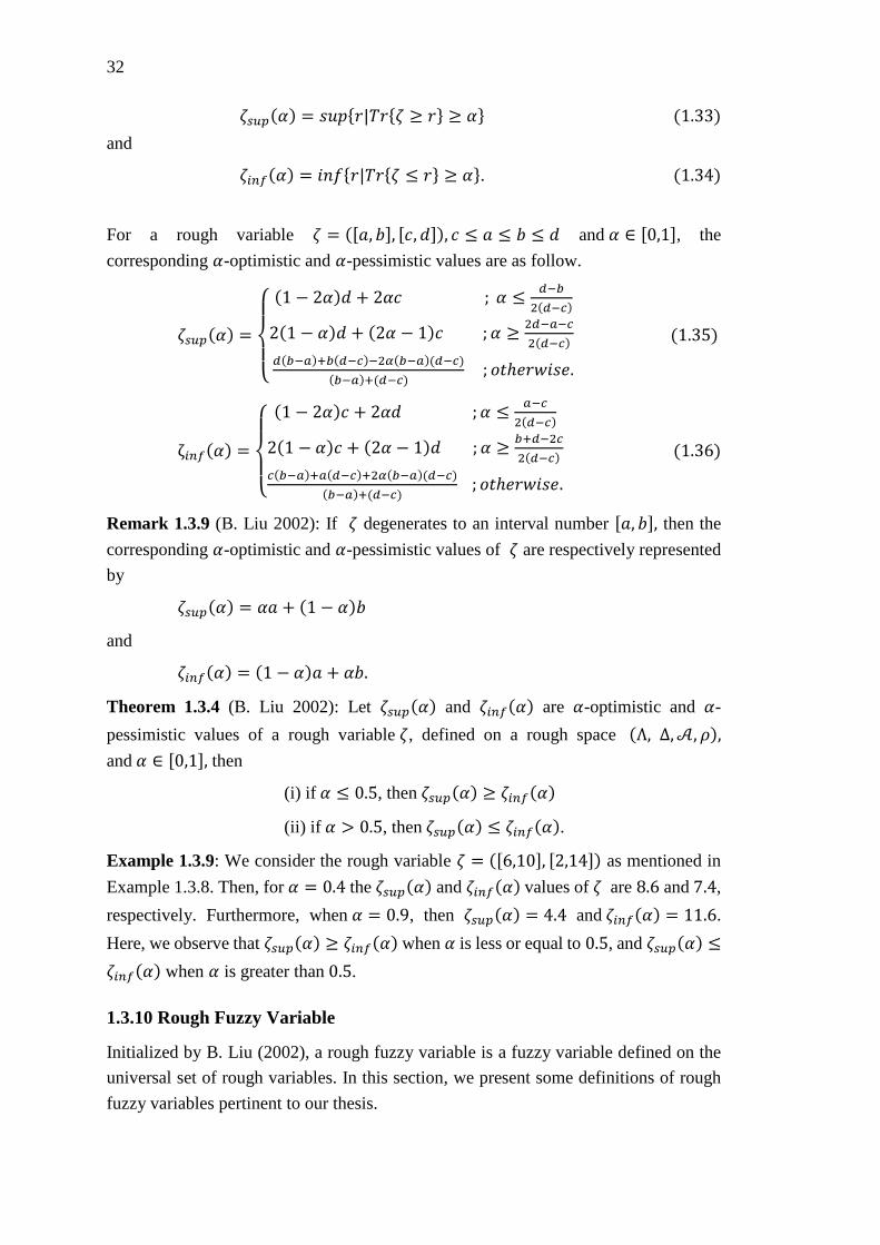
32

휁𝑠𝑢𝑝(𝛼) = 𝑠𝑢𝑝{𝑟|𝑇𝑟{휁 ≥ 𝑟} ≥ 𝛼} (1.33)

and

휁𝑖𝑛𝑓(𝛼) = 𝑖𝑛𝑓{𝑟|𝑇𝑟{휁 ≤ 𝑟} ≥ 𝛼}. (1.34)

For a rough variable 휁 = ([𝑎, 𝑏], [𝑐, 𝑑]), 𝑐 ≤ 𝑎 ≤ 𝑏 ≤ 𝑑 and 𝛼 ∈ [0,1], the

corresponding 𝛼-optimistic and 𝛼-pessimistic values are as follow.

휁𝑠𝑢𝑝(𝛼) =

{

(1 − 2𝛼)𝑑 + 2𝛼𝑐 ; 𝛼 ≤

𝑑−𝑏

2(𝑑−𝑐)

2(1 − 𝛼)𝑑 + (2𝛼 − 1)𝑐 ; 𝛼 ≥2𝑑−𝑎−𝑐

2(𝑑−𝑐)

𝑑(𝑏−𝑎)+𝑏(𝑑−𝑐)−2𝛼(𝑏−𝑎)(𝑑−𝑐)

(𝑏−𝑎)+(𝑑−𝑐) ; 𝑜𝑡ℎ𝑒𝑟𝑤𝑖𝑠𝑒.

(1.35)

ζ𝑖𝑛𝑓(𝛼) =

{

(1 − 2𝛼)𝑐 + 2𝛼𝑑 ; 𝛼 ≤

𝑎−𝑐

2(𝑑−𝑐)

2(1 − 𝛼)𝑐 + (2𝛼 − 1)𝑑 ; 𝛼 ≥𝑏+𝑑−2𝑐

2(𝑑−𝑐)

𝑐(𝑏−𝑎)+𝑎(𝑑−𝑐)+2𝛼(𝑏−𝑎)(𝑑−𝑐)

(𝑏−𝑎)+(𝑑−𝑐) ; 𝑜𝑡ℎ𝑒𝑟𝑤𝑖𝑠𝑒.

(1.36)

Remark 1.3.9 (B. Liu 2002): If 휁 degenerates to an interval number [𝑎, 𝑏], then the

corresponding 𝛼-optimistic and 𝛼-pessimistic values of 휁 are respectively represented

by

휁𝑠𝑢𝑝(𝛼) = 𝛼𝑎 + (1 − 𝛼)𝑏

and

휁𝑖𝑛𝑓(𝛼) = (1 − 𝛼)𝑎 + 𝛼𝑏.

Theorem 1.3.4 (B. Liu 2002): Let 휁𝑠𝑢𝑝(𝛼) and 휁𝑖𝑛𝑓(𝛼) are 𝛼-optimistic and 𝛼-

pessimistic values of a rough variable 휁, defined on a rough space (Ʌ, ∆,𝒜, 𝜌),

and 𝛼 ∈ [0,1], then

(i) if 𝛼 ≤ 0.5, then 휁𝑠𝑢𝑝(𝛼) ≥ 휁𝑖𝑛𝑓(𝛼)

(ii) if 𝛼 > 0.5, then 휁𝑠𝑢𝑝(𝛼) ≤ 휁𝑖𝑛𝑓(𝛼).

Example 1.3.9: We consider the rough variable 휁 = ([6,10], [2,14]) as mentioned in

Example 1.3.8. Then, for 𝛼 = 0.4 the 휁𝑠𝑢𝑝(𝛼) and 휁𝑖𝑛𝑓(𝛼) values of 휁 are 8.6 and 7.4,

respectively. Furthermore, when 𝛼 = 0.9, then 휁𝑠𝑢𝑝(𝛼) = 4.4 and 휁𝑖𝑛𝑓(𝛼) = 11.6.

Here, we observe that 휁𝑠𝑢𝑝(𝛼) ≥ 휁𝑖𝑛𝑓(𝛼) when 𝛼 is less or equal to 0.5, and 휁𝑠𝑢𝑝(𝛼) ≤

휁𝑖𝑛𝑓(𝛼) when 𝛼 is greater than 0.5.

1.3.10 Rough Fuzzy Variable

Initialized by B. Liu (2002), a rough fuzzy variable is a fuzzy variable defined on the

universal set of rough variables. In this section, we present some definitions of rough

fuzzy variables pertinent to our thesis.

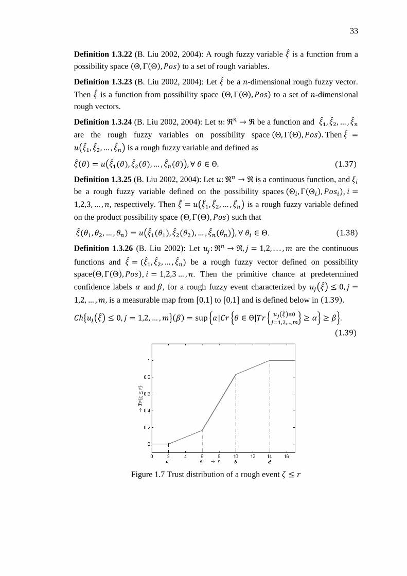
33

Definition 1.3.22 (B. Liu 2002, 2004): A rough fuzzy variable 𝜉 is a function from a

possibility space (Θ,Γ(Θ), 𝑃𝑜𝑠) to a set of rough variables.

Definition 1.3.23 (B. Liu 2002, 2004): Let 𝜉 be a 𝑛-dimensional rough fuzzy vector.

Then 𝜉 is a function from possibility space (Θ,Γ(Θ), 𝑃𝑜𝑠) to a set of 𝑛-dimensional

rough vectors.

Definition 1.3.24 (B. Liu 2002, 2004): Let 𝑢: ℜ𝑛 → ℜ be a function and 𝜉1, 𝜉2, … , 𝜉𝑛

are the rough fuzzy variables on possibility space (Θ,Γ(Θ), 𝑃𝑜𝑠). Then 𝜉 =

𝑢(𝜉1, 𝜉2, … , 𝜉𝑛) is a rough fuzzy variable and defined as

𝜉(휃) = 𝑢(𝜉1(휃), 𝜉2(휃), … , 𝜉𝑛(휃)), ∀ 휃 ∈ Θ. (1.37)

Definition 1.3.25 (B. Liu 2002, 2004): Let 𝑢: ℜ𝑛 → ℜ is a continuous function, and 𝜉𝑖

be a rough fuzzy variable defined on the possibility spaces (Θ𝑖,Γ(Θ𝑖), 𝑃𝑜𝑠𝑖), 𝑖 =

1,2,3, … , 𝑛, respectively. Then 𝜉 = 𝑢(𝜉1, 𝜉2, … , 𝜉𝑛) is a rough fuzzy variable defined

on the product possibility space (Θ,Γ(Θ), 𝑃𝑜𝑠) such that

𝜉(휃1, 휃2, … , 휃𝑛) = 𝑢(𝜉1(휃1), 𝜉2(휃2),… , 𝜉𝑛(휃𝑛)), ∀ 휃𝑖 ∈ Θ. (1.38)

Definition 1.3.26 (B. Liu 2002): Let 𝑢𝑗: ℜ𝑛 → ℜ, 𝑗 = 1,2, . . . , 𝑚 are the continuous

functions and 𝜉 = (𝜉1, 𝜉2, … , 𝜉𝑛) be a rough fuzzy vector defined on possibility

space(Θ,Γ(Θ), 𝑃𝑜𝑠), 𝑖 = 1,2,3… , 𝑛. Then the primitive chance at predetermined

confidence labels 𝛼 and 𝛽, for a rough fuzzy event characterized by 𝑢𝑗(𝜉) ≤ 0, 𝑗 =

1,2, … ,𝑚, is a measurable map from [0,1] to [0,1] and is defined below in (1.39).

𝐶ℎ{𝑢𝑗(𝜉) ≤ 0, 𝑗 = 1,2, … ,𝑚}(𝛽) = sup {𝛼|𝐶𝑟 {휃 ∈ Θ|𝑇𝑟 {𝑢𝑗(��)≤0

𝑗=1,2,…,𝑚} ≥ 𝛼} ≥ 𝛽}.

(1.39)

Figure 1.7 Trust distribution of a rough event 휁 ≤ 𝑟

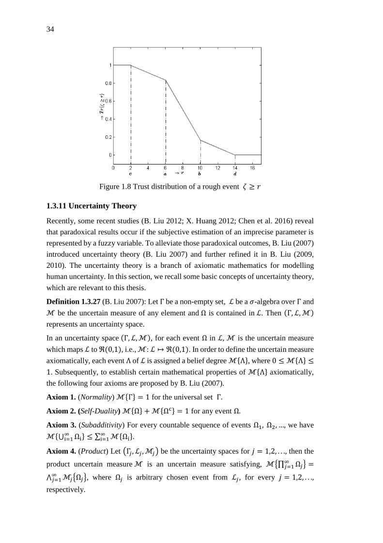
34

Figure 1.8 Trust distribution of a rough event 휁 ≥ 𝑟

1.3.11 Uncertainty Theory

Recently, some recent studies (B. Liu 2012; X. Huang 2012; Chen et al. 2016) reveal

that paradoxical results occur if the subjective estimation of an imprecise parameter is

represented by a fuzzy variable. To alleviate those paradoxical outcomes, B. Liu (2007)

introduced uncertainty theory (B. Liu 2007) and further refined it in B. Liu (2009,

2010). The uncertainty theory is a branch of axiomatic mathematics for modelling

human uncertainty. In this section, we recall some basic concepts of uncertainty theory,

which are relevant to this thesis.

Definition 1.3.27 (B. Liu 2007): Let Γ be a non-empty set, ℒ be a 𝜎-algebra over Γ and

ℳ be the uncertain measure of any element and Ω is contained in ℒ. Then (Γ, ℒ,ℳ)

represents an uncertainty space.

In an uncertainty space (Γ, ℒ,ℳ), for each event Ω in ℒ, ℳ is the uncertain measure

which maps ℒ to ℜ(0,1), i.e., ℳ: ℒ ↦ ℜ(0,1). In order to define the uncertain measure

axiomatically, each event Λ of ℒ is assigned a belief degree ℳ{Λ}, where 0 ≤ ℳ{Λ} ≤

1. Subsequently, to establish certain mathematical properties of ℳ{Λ} axiomatically,

the following four axioms are proposed by B. Liu (2007).

Axiom 1. (Normality) ℳ{Γ} = 1 for the universal set Γ.

Axiom 2. (Self-Duality) ℳ{Ω} +ℳ{Ωc} = 1 for any event Ω.

Axiom 3. (Subadditivity) For every countable sequence of events Ω1, Ω2, …, we have

ℳ{⋃ Ωi∞i=1 } ≤ ∑ ℳ{Ωi}.

∞i=1

Axiom 4. (Product) Let (Γ𝑗 , ℒ𝑗 ,ℳ𝑗) be the uncertainty spaces for 𝑗 = 1,2, . . ., then the

product uncertain measure ℳ is an uncertain measure satisfying, ℳ{∏ Ω𝑗∞𝑗=1 } =

⋀ ℳ𝑗{Ω𝑗}∞𝑗=1 , where Ω𝑗 is arbitrary chosen event from ℒ𝑗 , for every 𝑗 = 1,2, . . .,

respectively.

35

Definition 1.3.28 (B. Liu 2007): An uncertain variable ζ is a function from an

uncertainty space (Γ, ℒ,ℳ) to a set of real numbers ℜ, i.e., for any Borel set ℬ of ℜ

the set {ζ ∈ ℬ} in (1.40) is an event.

{ζ ∈ ℬ} = {γ ∈ Γ|ζ(γ) ∈ ℬ} (1.40)

Definition 1.3.29 (B. Liu 2007): An uncertain variable 휁 is said to be linear uncertain

variable if 휁 follows a linear uncertainty distribution as defined below.

Φ(𝑥) = {

0 ; 𝑖𝑓 𝑥 < 𝑎 𝑥−𝑎

𝑏−𝑎 ; 𝑖𝑓 𝑎 ≤ 𝑥 < 𝑏

1 ; 𝑖𝑓 𝑥 ≥ 𝑏,

(1.41)

where 휁 is denoted by ℒ(𝑎, 𝑏) such that 𝑎 < 𝑏 and 𝑎, 𝑏 ∈ ℜ.

Example 1.3.10: The uncertainty distribution of linear uncertainty variable ℒ(6,14) is

depicted in Fig. 1.9.

Figure 1.9 Linear uncertain distribution of ℒ(6,14)

Definition 1.3.30 (B. Liu 2007): An uncertain variable 휁 is said to be zigzag uncertain

variable if 휁 follows a zigzag uncertainty distribution as discussed in (1.42).

Φ(𝑥) =

{

0 ; 𝑖𝑓 𝑥 < 𝑎 𝑥−𝑎

2(𝑏−𝑎) ; 𝑖𝑓 𝑎 ≤ 𝑥 < 𝑏

(𝑥+𝑐−2𝑏)

2(𝑐−𝑏) ; 𝑖𝑓 𝑏 ≤ 𝑥 < 𝑐

1 ; 𝑖𝑓 𝑥 ≥ 𝑐,

(1.42)

where 휁 is denoted by 𝒵(𝑎, 𝑏, 𝑐) such that 𝑎 < 𝑏 < 𝑐 and 𝑎, 𝑏, 𝑐 ∈ ℜ.

Example 1.3.11: The uncertainty distribution of zigzag uncertain variable 𝒵(10,12,17)

is shown in Fig. 1.10.

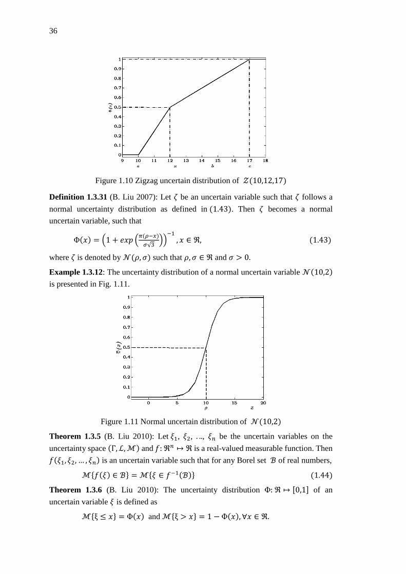
36

Figure 1.10 Zigzag uncertain distribution of 𝒵(10,12,17)

Definition 1.3.31 (B. Liu 2007): Let 휁 be an uncertain variable such that 휁 follows a

normal uncertainty distribution as defined in (1.43). Then 휁 becomes a normal

uncertain variable, such that

Φ(𝑥) = (1 + 𝑒𝑥𝑝 (𝜋(𝜌−𝑥)

𝜎√3))

−1

, 𝑥 ∈ ℜ, (1.43)

where 휁 is denoted by 𝒩(𝜌, 𝜎) such that 𝜌, 𝜎 ∈ ℜ and 𝜎 > 0.

Example 1.3.12: The uncertainty distribution of a normal uncertain variable 𝒩(10,2)

is presented in Fig. 1.11.

Figure 1.11 Normal uncertain distribution of 𝒩(10,2)

Theorem 1.3.5 (B. Liu 2010): Let 𝜉1, 𝜉2, . .., 𝜉𝑛 be the uncertain variables on the

uncertainty space (Γ, ℒ,ℳ) and 𝑓: ℜ𝑛 ↦ ℜ is a real-valued measurable function. Then

𝑓(𝜉1, 𝜉2, … , 𝜉𝑛) is an uncertain variable such that for any Borel set ℬ of real numbers,

ℳ{𝑓(𝜉) ∈ ℬ} = ℳ{𝜉 ∈ 𝑓−1(ℬ)} (1.44)

Theorem 1.3.6 (B. Liu 2010): The uncertainty distribution Φ: ℜ ↦ [0,1] of an

uncertain variable 𝜉 is defined as

ℳ{ξ ≤ 𝑥} = Φ(𝑥) and ℳ{ξ > 𝑥} = 1 − Φ(𝑥), ∀𝑥 ∈ ℜ.

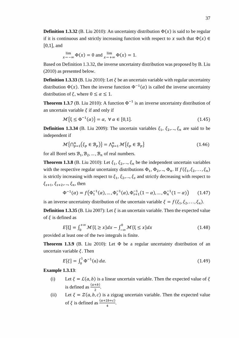
37

Definition 1.3.32 (B. Liu 2010): An uncertainty distribution Φ(𝑥) is said to be regular

if it is continuous and strictly increasing function with respect to 𝑥 such that Φ(𝑥) ∈

[0,1], and

lim

𝑥→ −∞Φ(𝑥) = 0 and

lim𝑥→ +∞

Φ(𝑥) = 1.

Based on Definition 1.3.32, the inverse uncertainty distribution was proposed by B. Liu

(2010) as presented below.

Definition 1.3.33 (B. Liu 2010): Let 𝜉 be an uncertain variable with regular uncertainty

distribution Φ(𝑥). Then the inverse function Φ−1(𝛼) is called the inverse uncertainty

distribution of 𝜉, where 0 ≤ 𝛼 ≤ 1.

Theorem 1.3.7 (B. Liu 2010): A function Φ−1 is an inverse uncertainty distribution of

an uncertain variable 𝜉 if and only if

ℳ{ξ ≤ Φ−1(𝛼)} = 𝛼, ∀ 𝛼 ∈ [0,1]. (1.45)

Definition 1.3.34 (B. Liu 2009): The uncertain variables 𝜉1, 𝜉2,. .., 𝜉𝑛 are said to be

independent if

ℳ{⋂ (𝜉𝑝 ∈ ℬ𝑝)𝑛𝑝=1 } = ⋀ ℳ{𝜉𝑝 ∈ ℬ𝑝}

𝑛𝑝=1 (1.46)

for all Borel sets ℬ1, ℬ2, … , ℬ𝑛 of real numbers.

Theorem 1.3.8 (B. Liu 2010): Let 𝜉1, 𝜉2,. .., 𝜉𝑛 be the independent uncertain variables

with the respective regular uncertainty distributions Φ1, Φ2,. .., Φ𝑛. If 𝑓(𝜉1, 𝜉2, . . . , 𝜉𝑛)

is strictly increasing with respect to 𝜉1, 𝜉2,. .., 𝜉𝑠 and strictly decreasing with respect to

𝜉𝑠+1, 𝜉𝑠+2,. .., 𝜉𝑛, then

Φ−1(𝛼) = 𝑓(Φ1−1(𝛼),… ,Φ𝑠

−1(𝛼),Φ𝑠+1−1 (1 − 𝛼),… ,Φ𝑛

−1(1 − 𝛼)) (1.47)

is an inverse uncertainty distribution of the uncertain variable 𝜉 = 𝑓(𝜉1, 𝜉2, . . . , 𝜉𝑛).

Definition 1.3.35 (B. Liu 2007): Let 𝜉 is an uncertain variable. Then the expected value

of 𝜉 is defined as

𝐸[ξ] = ∫ ℳ{ξ ≥ 𝑥}𝑑𝑥+∞

0− ∫ ℳ{ξ ≤ 𝑥}𝑑𝑥

0

−∞ (1.48)

provided at least one of the two integrals is finite.

Theorem 1.3.9 (B. Liu 2010): Let Φ be a regular uncertainty distribution of an

uncertain variable 𝜉. Then

𝐸[𝜉] = ∫ Φ−1(α)1

0𝑑𝛼. (1.49)

Example 1.3.13:

(i) Let 𝜉 = ℒ(𝑎, 𝑏) is a linear uncertain variable. Then the expected value of 𝜉

is defined as (𝑎+𝑏)

2.

(ii) Let 𝜉 = 𝒵(𝑎, 𝑏, 𝑐) is a zigzag uncertain variable. Then the expected value

of 𝜉 is defined as (𝑎+2𝑏+𝑐)

4.

38

(iii) Let 𝜉 = 𝒩(𝑚, 𝜎) is a normal uncertain variable. Then the expected value

of 𝜉 is defined as 𝑚.

Theorem 1.3.10 (B. Liu 2010): Let 𝜉1 and 𝜉2 are the independent uncertain variables

with finite expected values. Then for any real numbers 𝑎 and 𝑏, we have

𝐸[𝑎𝜉1 + 𝑏𝜉2] = 𝑎𝐸[𝜉1] + 𝑏𝐸[𝜉2]. (1.50)

Theorem 1.3.11 (Liu and Ha 2010): Let 𝜉1, 𝜉2,. .., 𝜉𝑛 be the independent uncertain

variables with the respective regular uncertainty distributions Φ1, Φ2,. .., Φ𝑛. If 𝜉 =

𝑓(𝜉1, 𝜉2, . . . , 𝜉𝑛) is strictly increasing with respect to 𝜉1, 𝜉2,. .., 𝜉𝑠 and strictly decreasing

with respect to 𝜉𝑠+1, 𝜉𝑠+2,. .., 𝜉𝑛, then

𝐸[𝜉] = ∫ 𝑓(Φ1−1(𝛼),… ,Φ𝑠

−1(𝛼),Φ𝑠+1−1 (1 − 𝛼),… ,Φ𝑛

−1(1 − 𝛼))𝑑𝛼1

0 (1.51)

is the expected value of the uncertain variable 𝜉 = 𝑓(𝜉1, 𝜉2, . . . , 𝜉𝑛).

Definition 1.3.36 (B. Liu 2007): Let 휁 be an uncertain variable and 𝛼 ∈ (0,1] be the

confidence level, then 휁𝑠𝑢𝑝(𝛼) and 휁𝑖𝑛𝑓(𝛼) are the respective 𝛼-optimistic and 𝛼-

pessimistic values of 휁 such that

휁𝑠𝑢𝑝(𝛼) = 𝑠𝑢𝑝{𝑡|ℳ{휁 ≥ 𝑡} ≥ 𝛼} (1.52)

and

휁𝑖𝑛𝑓(𝛼) = 𝑖𝑛𝑓{𝑡|ℳ{휁 ≤ 𝑡} ≥ 𝛼} (1.53)

Example 1.3.14

(i) Let 휁 be a linear uncertain variable ℒ(𝑎, 𝑏), then the corresponding 𝛼-optimistic

and 𝛼-pessimistic values of 휁 are respectively

휁𝑠𝑢𝑝(𝛼) = 𝛼𝑎 + (1 − 𝛼)𝑏

and

휁𝑖𝑛𝑓(𝛼) = (1 − 𝛼)𝑎 + 𝛼𝑏.

(ii) Let 휁 be a zigzag uncertain variable 𝒵(𝑎, 𝑏, 𝑐), then 𝛼-optimistic and 𝛼-

pessimistic values are respectively

휁𝑠𝑢𝑝(𝛼) = {2𝛼𝑏 + (1 − 2𝛼)𝑐 ; 𝑖𝑓 𝛼 < 0.5(2𝛼 − 1)𝑎 + (2 − 2𝛼)𝑏 ; 𝑖𝑓 𝛼 ≥ 0.5

and

휁𝑖𝑛𝑓(𝛼) = {(1 − 2𝛼)𝑎 + 2𝛼𝑏 ; 𝑖𝑓 𝛼 < 0.5(2 − 2𝛼)𝑏 + (2𝛼 − 1)𝑐 ; 𝑖𝑓 𝛼 ≥ 0.5.

(iii) Let 휁 be a normal uncertain variable 𝒩(𝜌, 𝜎) then the respective 𝛼-optimistic

and 𝛼-pessimistic values of 휁 are respectively

휁𝑠𝑢𝑝(𝛼) = 𝜌 −𝜎√3

𝜋𝑙𝑛

𝛼

1−𝛼

and

39

휁𝑖𝑛𝑓(𝛼) = 𝜌 +𝜎√3

𝜋𝑙𝑛

𝛼

1−𝛼·

1.3.12 Ordered Weighted Averaging (OWA) Operator

In this section, we present the concept of ordered weighted averaging operator and one

of its variant, the argument-dependent approach of OWA operator.

Definition 1.3.37 (R.R. Yager 1988): An OWA operator of dimension 𝑛 is a mapping,

OWA: ℜ𝑛 ↦ ℜ, which has an associated weight vector, (=

[1,2, … ,𝑛]𝑇) ∀𝑖∈[0,1] and ∑ 𝑖 = 1.

𝑛𝑖=1

Moreover, OWA(𝑏1, 𝑏2, … , 𝑏𝑛) = ∑ 𝑖𝑏𝜋(𝑖),𝑛𝑖=1

where (𝑏1, 𝑏2, … , 𝑏𝑛) is the collection of 𝑛 arguments and {𝜋(1), 𝜋(2),… , 𝜋(𝑛)} is a

permutation of {1,2, … , 𝑛} such that 𝑏𝜋(𝑖−1) ≥ 𝑏𝜋(𝑖) ∀𝑖 ∈ {2,3, … , 𝑛}.

Argument-dependent approach for 𝐎𝐖𝐀 Weights

Z. Xu (2006) proposed an argument-dependent approach to determine the OWA

weights which are defined as follows.

For an argument list 𝐵 = (𝑏1, 𝑏2, … , 𝑏𝑛), let 𝜇 (=∑ 𝑏𝑖𝑛𝑖=1

𝑛) be the mean of 𝐵 and

{𝜋(1), 𝜋(2), … , 𝜋(𝑛)} be a permutation of {1,2, … , 𝑛} such that 𝑏𝜋(𝑖−1) ≥ 𝑏𝜋(𝑖) ∀𝑖 ∈

{2,3, … , 𝑛}. Then the similarity degree 𝑠(𝑏𝜋(𝑖), 𝜇) for 𝑖𝑡ℎ largest argument 𝑏𝜋(𝑖) is given

by

𝑠(𝑏𝜋(𝑖), 𝜇) = 1 −|𝑏𝜋(𝑖)−𝜇|

∑ |𝑏𝑖−𝜇|𝑛𝑖=1

∀𝑖 = 1,2, … , 𝑛. (1.54)

If (= [1,2, … ,𝑛]𝑇) is the weight vector of OWA operator then we define each 𝑖

as

𝑖 =𝑠(𝑏𝜋(𝑖),𝜇)

∑ 𝑠(𝑏𝜋(𝑖),𝜇)𝑛𝑖=1

∀𝑖 = 1,2, … , 𝑛. (1.55)

Henceforth,

OWA(𝑏1, 𝑏2, … , 𝑏𝑛) =∑ (𝑠(𝑏𝜋(𝑖),𝜇)×𝑏𝜋(𝑖))𝑛𝑖=1

∑ 𝑠(𝑏𝜋(𝑖),𝜇)𝑛𝑖=1

. (1.56)

Example 1.3.15

Consider an argument list 𝐵 as presented below.

𝐵=[37.9647, 23.5676, 47.90,22.7985,54.2456]

Let {𝜋(1), 𝜋(2), 𝜋(3), 𝜋(4), 𝜋(5)} be a permutation of {1,2,3,4,5} such that 𝑏𝜋(𝑖−1) ≥

𝑏𝜋(𝑖), 𝑖 = 2,3, … ,5 and 𝑏𝜋(𝑖) is an element of 𝐵. Then, arranging the elements of 𝐵

as,𝑏𝜋(1) = 54.2456,𝑏𝜋(2) = 47.90,𝑏𝜋(3) = 37.9647,𝑏𝜋(4) = 23.5676 and 𝑏𝜋(5) =

22.7985. We calculate the mean of the elements of 𝐵 as

40

𝜇 =(37.9647+ 23.5676+ 47.90+22.7985+54.2456)

5= 37.2953.

Now we can find all the 𝑖 of the corresponding weight vector, for 𝐵 following

(1.50) and (1.51) as follows.

So, 𝑠(𝑏𝜋(1), 37.2953) =

1 −|54.2456−37.2953|

(|37.9647−37.2953|+|23.5676−37.2953|+|47.90−37.2953|+|22.7985−37.2953|+|54.2456−37.2953|)

= 0.6997

Similarly, 𝑠(𝑏𝜋(2), 37.2953) = 0.8121, 𝑠(𝑏𝜋(3), 37.2953) = 0.9881,

𝑠(𝑏𝜋(4), 37.2953) = 0.7568 and 𝑠(𝑏𝜋(5), 37.2953) = 0.7432.

Furthermore, 1 =0.6997

(0.6997+0.8121+0.9881+0.7568+0.7432)= 0.1749.

Correspondingly, 2 = 0.2030,3 = 0.2470,4 = 0.1892 and 5 = 0.1858.

Therefore, according to (1.52), OWA(37.9647, 23.5676, 47.90,22.7985,54.2456)

= (0.1749 × 54.2456 + 0.2030 × 47.90 + 0.2470 × 37.9647 + 0.1892 ×

23.5676 + 0.1858 × 22.7985) = 37.2835.

1.3.13 Single objective Optimization

The problem of optimization concerns with the maximization/minimization of an

algebraic or a transcendental function of one or more variables, known as objective

function, under some available resources which are represented as constraints. Such a

problem is called a single objective optimization problem which is formulated as

follows.

{

𝑀𝑖𝑛𝑖𝑚𝑖𝑧𝑒 𝑧(𝑥) 𝑠𝑢𝑏𝑗𝑒𝑐𝑡 𝑡𝑜

𝑔𝑗(𝑥) ≤ 0; 𝑗 = 1, 2, … ,𝑚

ℎ𝑘(𝑥) = 0; 𝑘 = 1, 2, … , 𝑝

𝑥 = (𝑥1, 𝑥2, … , 𝑥𝑛)𝑇 ∈ ℜ𝑛,

(1.57)

where 𝑥 is an 𝑛-dimensional decision vector, 𝑧(𝑥), 𝑔𝑗(𝑥) and ℎ𝑘(𝑥) are respectively

the objective function, set of inequality constraints and equality constraints defined on

𝑥. A decision vector satisfying all the constraints of the above Single objective

optimization problem (SOOP) is called a feasible solution of (1.57). The collection of

all such solutions forms the feasible region. The aim of a SOOP problem is to find a

feasible solution 𝑥∗ such that for each feasible solution, 𝑧(𝑥) ≤ 𝑧(𝑥∗) for maximization

problem and 𝑧(𝑥) ≥ 𝑧( 𝑥∗) for minimization problem. Here, 𝑥∗ is called an optimal

solution of (1.57).

1.3.14 Multi-objective Optimization (MOP)

An MOP optimizes a vector of conflicting objectives, which can be formulated as

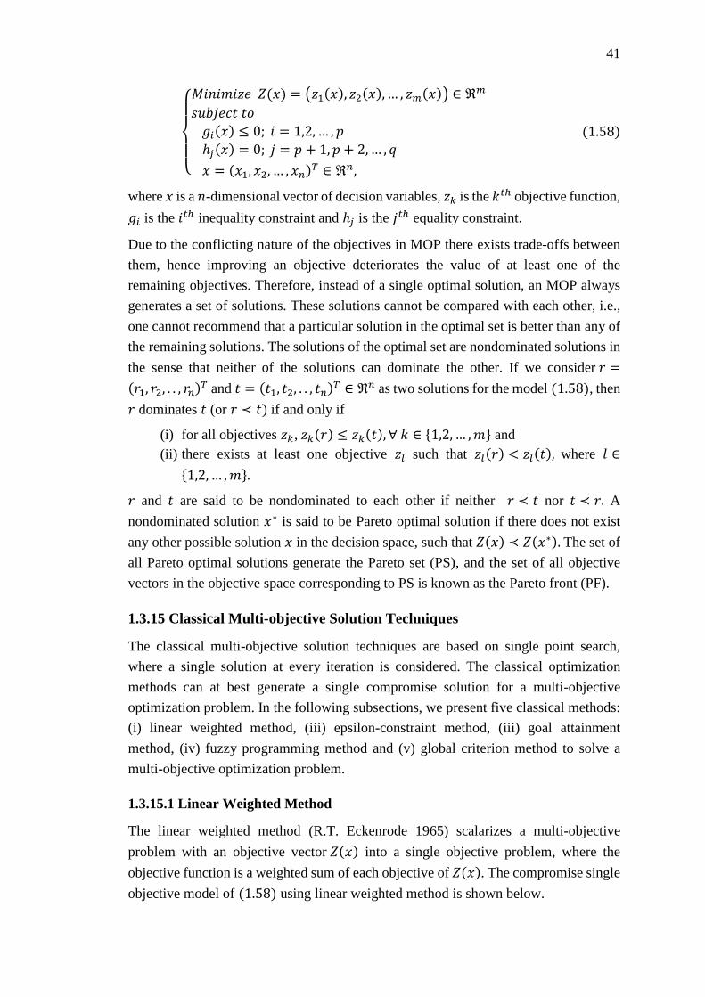
41

{

𝑀𝑖𝑛𝑖𝑚𝑖𝑧𝑒 𝑍(𝑥) = (𝑧1(𝑥), 𝑧2(𝑥),… , 𝑧𝑚(𝑥)) ∈ ℜ

𝑚

𝑠𝑢𝑏𝑗𝑒𝑐𝑡 𝑡𝑜

𝑔𝑖(𝑥) ≤ 0; 𝑖 = 1,2, … , 𝑝

ℎ𝑗(𝑥) = 0; 𝑗 = 𝑝 + 1, 𝑝 + 2,… , 𝑞

𝑥 = (𝑥1, 𝑥2, … , 𝑥𝑛)𝑇 ∈ ℜ𝑛,

(1.58)

where 𝑥 is a 𝑛-dimensional vector of decision variables, 𝑧𝑘 is the 𝑘𝑡ℎ objective function,

𝑔𝑖 is the 𝑖𝑡ℎ inequality constraint and ℎ𝑗 is the 𝑗𝑡ℎ equality constraint.

Due to the conflicting nature of the objectives in MOP there exists trade-offs between

them, hence improving an objective deteriorates the value of at least one of the

remaining objectives. Therefore, instead of a single optimal solution, an MOP always

generates a set of solutions. These solutions cannot be compared with each other, i.e.,

one cannot recommend that a particular solution in the optimal set is better than any of

the remaining solutions. The solutions of the optimal set are nondominated solutions in

the sense that neither of the solutions can dominate the other. If we consider 𝑟 =

(𝑟1, 𝑟2, . . , 𝑟𝑛)𝑇 and 𝑡 = (𝑡1, 𝑡2, . . , 𝑡𝑛)

𝑇 ∈ ℜ𝑛 as two solutions for the model (1.58), then

𝑟 dominates 𝑡 (or 𝑟 ≺ 𝑡) if and only if

(i) for all objectives 𝑧𝑘, 𝑧𝑘(𝑟) ≤ 𝑧𝑘(𝑡), ∀ 𝑘 ∈ {1,2, … ,𝑚} and

(ii) there exists at least one objective 𝑧𝑙 such that 𝑧𝑙(𝑟) < 𝑧𝑙(𝑡), where 𝑙 ∈

{1,2, … ,𝑚}.

𝑟 and 𝑡 are said to be nondominated to each other if neither 𝑟 ≺ 𝑡 nor 𝑡 ≺ 𝑟. A

nondominated solution 𝑥∗ is said to be Pareto optimal solution if there does not exist

any other possible solution 𝑥 in the decision space, such that 𝑍(𝑥) ≺ 𝑍(𝑥∗). The set of

all Pareto optimal solutions generate the Pareto set (PS), and the set of all objective

vectors in the objective space corresponding to PS is known as the Pareto front (PF).

1.3.15 Classical Multi-objective Solution Techniques

The classical multi-objective solution techniques are based on single point search,

where a single solution at every iteration is considered. The classical optimization

methods can at best generate a single compromise solution for a multi-objective

optimization problem. In the following subsections, we present five classical methods:

(i) linear weighted method, (iii) epsilon-constraint method, (iii) goal attainment

method, (iv) fuzzy programming method and (v) global criterion method to solve a

multi-objective optimization problem.

1.3.15.1 Linear Weighted Method

The linear weighted method (R.T. Eckenrode 1965) scalarizes a multi-objective

problem with an objective vector 𝑍(𝑥) into a single objective problem, where the

objective function is a weighted sum of each objective of 𝑍(𝑥). The compromise single

objective model of (1.58) using linear weighted method is shown below.

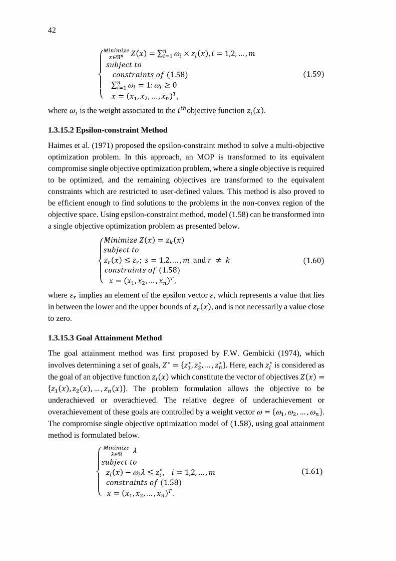
42

{

𝑀𝑖𝑛𝑖𝑚𝑖𝑧𝑒𝑥∈ℜ𝑛

𝑍(𝑥) = ∑ 𝑖 × 𝑧𝑖(𝑥), 𝑖 = 1,2, … ,𝑚 𝑛𝑖=1

𝑠𝑢𝑏𝑗𝑒𝑐𝑡 𝑡𝑜 𝑐𝑜𝑛𝑠𝑡𝑟𝑎𝑖𝑛𝑡𝑠 𝑜𝑓 (1.58)

∑ 𝑖 = 1:𝑖 ≥ 0𝑛 𝑖=1

𝑥 = (𝑥1, 𝑥2, … , 𝑥𝑛)𝑇 ,

(1.59)

where 𝜔𝑖 is the weight associated to the 𝑖𝑡ℎobjective function 𝑧𝑖(𝑥).

1.3.15.2 Epsilon-constraint Method

Haimes et al. (1971) proposed the epsilon-constraint method to solve a multi-objective

optimization problem. In this approach, an MOP is transformed to its equivalent

compromise single objective optimization problem, where a single objective is required

to be optimized, and the remaining objectives are transformed to the equivalent

constraints which are restricted to user-defined values. This method is also proved to

be efficient enough to find solutions to the problems in the non-convex region of the

objective space. Using epsilon-constraint method, model (1.58) can be transformed into

a single objective optimization problem as presented below.

{

𝑀𝑖𝑛𝑖𝑚𝑖𝑧𝑒 𝑍(𝑥) = 𝑧𝑘(𝑥) 𝑠𝑢𝑏𝑗𝑒𝑐𝑡 𝑡𝑜

𝑧𝑟(𝑥) ≤ 휀𝑟; 𝑠 = 1,2, … ,𝑚 and 𝑟 ≠ 𝑘 𝑐𝑜𝑛𝑠𝑡𝑟𝑎𝑖𝑛𝑡𝑠 𝑜𝑓 (1.58)

𝑥 = (𝑥1, 𝑥2, … , 𝑥𝑛)𝑇 ,

(1.60)

where 휀𝑟 implies an element of the epsilon vector 휀, which represents a value that lies

in between the lower and the upper bounds of 𝑧𝑟(𝑥), and is not necessarily a value close

to zero.

1.3.15.3 Goal Attainment Method

The goal attainment method was first proposed by F.W. Gembicki (1974), which

involves determining a set of goals, 𝑍∗ = {𝑧1∗, 𝑧2

∗, … , 𝑧𝑛∗}. Here, each 𝑧𝑖

∗ is considered as

the goal of an objective function 𝑧𝑖(𝑥) which constitute the vector of objectives 𝑍(𝑥) =

{𝑧1(𝑥), 𝑧2(𝑥),… , 𝑧𝑛(𝑥)}. The problem formulation allows the objective to be

underachieved or overachieved. The relative degree of underachievement or

overachievement of these goals are controlled by a weight vector = {1,2, … ,𝑛}.

The compromise single objective optimization model of (1.58), using goal attainment

method is formulated below.

{

𝑀𝑖𝑛𝑖𝑚𝑖𝑧𝑒𝜆∈ℜ

𝜆


𝑧𝑖(𝑥) − 𝑖𝜆 ≤ 𝑧𝑖∗, 𝑖 = 1,2, … ,𝑚

𝑐𝑜𝑛𝑠𝑡𝑟𝑎𝑖𝑛𝑡𝑠 𝑜𝑓 (1.58)

𝑥 = (𝑥1, 𝑥2, … , 𝑥𝑛)𝑇 .

(1.61)

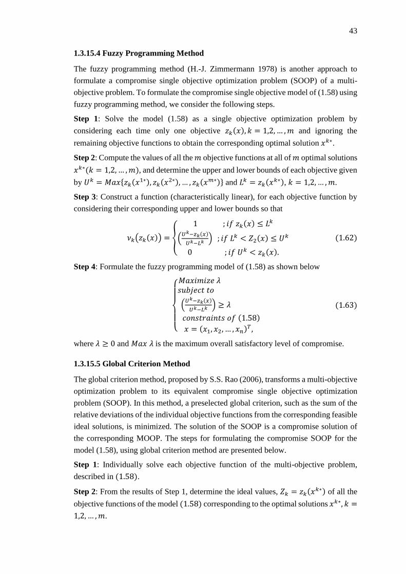
43

1.3.15.4 Fuzzy Programming Method

The fuzzy programming method (H.-J. Zimmermann 1978) is another approach to

formulate a compromise single objective optimization problem (SOOP) of a multi-

objective problem. To formulate the compromise single objective model of (1.58) using

fuzzy programming method, we consider the following steps.

Step 1: Solve the model (1.58) as a single objective optimization problem by

considering each time only one objective 𝑧𝑘(𝑥), 𝑘 = 1,2, … ,𝑚 and ignoring the

remaining objective functions to obtain the corresponding optimal solution 𝑥𝑘∗.

Step 2: Compute the values of all the 𝑚 objective functions at all of 𝑚 optimal solutions

𝑥𝑘∗(𝑘 = 1,2, … ,𝑚), and determine the upper and lower bounds of each objective given

by 𝑈𝑘 = 𝑀𝑎𝑥{𝑧𝑘(𝑥1∗), 𝑧𝑘(𝑥

2∗), … , 𝑧𝑘(𝑥𝑚∗)} and 𝐿𝑘 = 𝑧𝑘(𝑥

𝑘∗), 𝑘 = 1,2, … ,𝑚.

Step 3: Construct a function (characteristically linear), for each objective function by

considering their corresponding upper and lower bounds so that

𝜈𝑘(𝑧𝑘(𝑥)) = {

1 ; 𝑖𝑓 𝑧𝑘(𝑥) ≤ 𝐿𝑘

(𝑈𝑘−𝑧𝑘(𝑥)

𝑈𝑘−𝐿𝑘) ; 𝑖𝑓 𝐿𝑘 < 𝑍2(𝑥) ≤ 𝑈

𝑘

0 ; 𝑖𝑓 𝑈𝑘 < 𝑧𝑘(𝑥).

(1.62)

Step 4: Formulate the fuzzy programming model of (1.58) as shown below

{

𝑀𝑎𝑥𝑖𝑚𝑖𝑧𝑒 𝜆 𝑠𝑢𝑏𝑗𝑒𝑐𝑡 𝑡𝑜

(𝑈𝑘−𝑧𝑘(𝑥)

𝑈𝑘−𝐿𝑘) ≥ 𝜆


𝑥 = (𝑥1, 𝑥2, … , 𝑥𝑛)𝑇 ,

(1.63)

where 𝜆 ≥ 0 and 𝑀𝑎𝑥 𝜆 is the maximum overall satisfactory level of compromise.

1.3.15.5 Global Criterion Method

The global criterion method, proposed by S.S. Rao (2006), transforms a multi-objective

optimization problem to its equivalent compromise single objective optimization

problem (SOOP). In this method, a preselected global criterion, such as the sum of the

relative deviations of the individual objective functions from the corresponding feasible

ideal solutions, is minimized. The solution of the SOOP is a compromise solution of

the corresponding MOOP. The steps for formulating the compromise SOOP for the

model (1.58), using global criterion method are presented below.

Step 1: Individually solve each objective function of the multi-objective problem,

described in (1.58).

Step 2: From the results of Step 1, determine the ideal values, 𝑍𝑘 = 𝑧𝑘(𝑥𝑘∗) of all the

objective functions of the model (1.58) corresponding to the optimal solutions 𝑥𝑘∗, 𝑘 =

1,2, … ,𝑚.

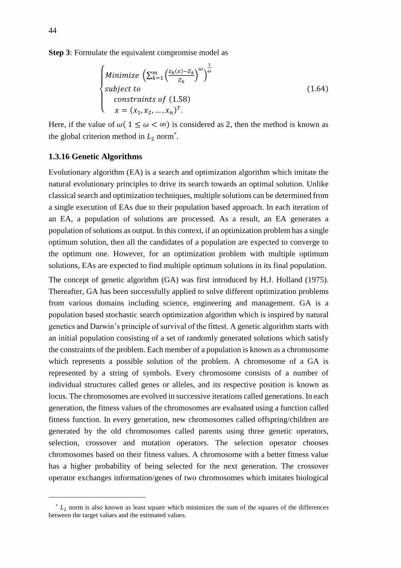
44

Step 3: Formulate the equivalent compromise model as

{

𝑀𝑖𝑛𝑖𝑚𝑖𝑧𝑒 (∑ (

𝑧𝑘(𝑥)−𝑍𝑘

𝑍𝑘)𝜔

𝑚𝑘=1 )

1

𝜔



𝑥 = (𝑥1, 𝑥2, … , 𝑥𝑛)𝑇 .

(1.64)

Here, if the value of 𝜔( 1 ≤ 𝜔 < ∞) is considered as 2, then the method is known as

the global criterion method in 𝐿2 norm*.

1.3.16 Genetic Algorithms

Evolutionary algorithm (EA) is a search and optimization algorithm which imitate the

natural evolutionary principles to drive its search towards an optimal solution. Unlike

classical search and optimization techniques, multiple solutions can be determined from

a single execution of EAs due to their population based approach. In each iteration of

an EA, a population of solutions are processed. As a result, an EA generates a

population of solutions as output. In this context, if an optimization problem has a single

optimum solution, then all the candidates of a population are expected to converge to

the optimum one. However, for an optimization problem with multiple optimum

solutions, EAs are expected to find multiple optimum solutions in its final population.

The concept of genetic algorithm (GA) was first introduced by H.J. Holland (1975).

Thereafter, GA has been successfully applied to solve different optimization problems

from various domains including science, engineering and management. GA is a

population based stochastic search optimization algorithm which is inspired by natural

genetics and Darwin’s principle of survival of the fittest. A genetic algorithm starts with

an initial population consisting of a set of randomly generated solutions which satisfy

the constraints of the problem. Each member of a population is known as a chromosome

which represents a possible solution of the problem. A chromosome of a GA is

represented by a string of symbols. Every chromosome consists of a number of

individual structures called genes or alleles, and its respective position is known as

locus. The chromosomes are evolved in successive iterations called generations. In each

generation, the fitness values of the chromosomes are evaluated using a function called

fitness function. In every generation, new chromosomes called offspring/children are

generated by the old chromosomes called parents using three genetic operators,

selection, crossover and mutation operators. The selection operator chooses

chromosomes based on their fitness values. A chromosome with a better fitness value

has a higher probability of being selected for the next generation. The crossover

operator exchanges information/genes of two chromosomes which imitates biological

* 𝐿2 norm is also known as least square which minimizes the sum of the squares of the differences

between the target values and the estimated values.

45

recombination process between two single chromosome organisms. A mutation

operator randomly changes the allele value(s) of chromosome. Finally, after several

generations, when a termination criterion (maximum generation, unchanged population

for 𝑛 successive generations, etc.) of a GA is reached, the algorithm is expected to

converge to the best chromosome which essentially represents an optimal or sub-

optimal solution of the problem.

A genetic algorithm for a particular optimization problem must have the following six

components.

(i) Genetic representation of the potential solutions to the problem, called

chromosomes.

(ii) A way to generate an initial population of potential solutions by satisfying the

problem constraints, may be randomly generated.

(iii) An objective function to evaluate the fitness of each solution/chromosome.

(iv) The genetic operator (selection) which select the chromosomes with better

fitness values.

(v) The genetic operators (crossover and mutation) which modify the composition

of chromosomes.

(vi) Values of different associated parameters of a genetic algorithm (population

size, crossover probability, mutation probability, etc.).

An algorithm for a simple GA is presented below.

begin

𝑡 = 0; // first generation

Generate (𝑃(0)) // initial population

evaluate (𝑃(𝑡))

while (termination_criterion is not reached) do

𝑅(𝑡) = selection(𝑃(𝑡))

𝑅(𝑡) = crossover(𝑅(𝑡))

𝑅(𝑡) = mutation(𝑅(𝑡))

𝑃(𝑡) = 𝑅(𝑡)

evaluate (𝑃(𝑡)) // evaluate the fitness of the chromosomes in the

// population P(t)

𝑡= 𝑡 + 1

end while

return the best solution

end

In this thesis, we have considered both single and multi-objective GAs for some of our

studies. Specifically, we have used a modified version of a genetic algorithm (GA) as

a solution methodology for a single objective problem (cf. Section 3.4 in Chapter 3).

While, for some multi-objective problems, we have employed two multi-objective

46

genetic algorithms (MOGAs): nondominated sorting genetic algorithm II (NSGA-II)

(Deb et al. 2002) and multi-objective cross generational elitist selection, heterogeneous

recombination and cataclysmic mutation (MOCHC) (Nebro et al. 2007). Accordingly,

the working principles of these MOGAs are discused in subsequent subsections.

1.3.16.1 Nondominated Sorting Genetic Algorithm II (NSGA-II)

The nondominated sorting genetic algorithm II (NSGA-II), proposed by Deb et al.

(2002), is an elitist multi-objective genetic algorithm, which ensures retaining the fittest

candidates in the next population to enhance the convergence. The algorithm starts with

initializing a population 𝑃0 of 𝑁 randomly generated solutions. In a particular

generation 𝑡, the genetic operators, i.e., selection, crossover and mutation are applied

on the individuals of parent population 𝑃𝑡 to generate an offspring population 𝐶𝑡 having

equal number of candidate solutions as parent population. To ensure elitism, the parent

and offspring population are mingled to produce a population 𝑆𝑡 of size 2𝑁. In order to

select 𝑁 best solutions from 𝑆𝑡 for next generation, NSGA-II performs following two

steps.

Sorting based on Rank: It frontifies the individuals of 𝑆𝑡, by assigning a rank to each

individual solution, i.e., a solution 𝑝 is assigned a rank 𝑝𝑟𝑎𝑛𝑘. Based on their ranks, the

solutions in 𝑆𝑡 are frontified to different nondominated fronts 𝑁1, 𝑁2,. .., 𝑁𝑙. Each

𝑁𝑘, 𝑘 ∈ {1,2, … , 𝑙} represents a set of nondominated solutions of rank 𝑘. Solutions with

the same rank value are placed in a nondominated front. Solutions with lower

nondomination ranks is always preferred. In other words, if 𝑝 and 𝑞 are the two

solutions in 𝑆𝑡, and if 𝑝𝑟𝑎𝑛𝑘 < 𝑞𝑟𝑎𝑛𝑘, then 𝑝 is superior to 𝑞. In order to build the next

population 𝑃𝑡+1, the solutions belonging to 𝑁1 are considered first. Here, if the size of

𝑁1 is less than 𝑁, all the solutions of 𝑁1 are inserted in 𝑃𝑡+1. The remaining solutions

of 𝑃𝑡+1 are considered from subsequent nondominated fronts in order of their ranking.

In this way, the solutions of 2nd front, i.e., 𝑁2 are moved next to 𝑃𝑡+1 followed by

solutions of 𝑁3 and so on until all the solutions of a nondominated front 𝑁𝑘 cannot be

fully inserted to 𝑃𝑡+1.

Sorting based on Crowding Distance: If all the solutions of 𝑁𝑘 cannot be

accommodated in 𝑃𝑡+1, the solutions are then sorted in descending order based on their

corresponding values of crowding distance (a solution 𝑖 in 𝑁𝑘 is assigned 𝑖𝑑𝑖𝑠𝑡𝑎𝑛𝑐𝑒) as

proposed by Deb et al. (2002). Particularly, if p and q are the two nondominated

solutions belong to 𝑁𝑘 and 𝑝 has better crowding distance than 𝑞, i.e., if 𝑝𝑟𝑎𝑛𝑘 = 𝑞𝑟𝑎𝑛𝑘

and 𝑝𝑑𝑖𝑠𝑡𝑎𝑛𝑐𝑒 > 𝑞𝑑𝑖𝑠𝑡𝑎𝑛𝑐𝑒, then 𝑝 is preferred over 𝑞 in 𝑁𝑘. Accordingly, the solutions

with higher crowding distance are eventually selected from 𝑁𝑘 to fill the remaining

slots of 𝑃𝑡+1.

47

In this way, as the formation of 𝑃𝑡+1 completes, the individuals of 𝑃𝑡+1 replaces 𝑃𝑡 for

the next generation. This process is continued until the termination condition (i.e.,

maximum function evaluations or generations) is reached.

1.3.16.2 Multi-objective Cross Generational Elitist Selection, Heterogeneous

Recombination and Cataclysmic Mutation (MOCHC)

Nebro et al. (2007) presented MOCHC as a multi-objective version of cross

generational elitist selection, heterogeneous selection and cataclysmic mutation (CHC)

algorithm (L.J. Eshelman 1991). MOCHC begins its execution by randomly generating

an initial population 𝑃0 of size 𝑁. At every subsequent generation 𝑡, a set of solutions

in 𝑃𝑡 is generated by randomly selecting a pair of parent solutions from 𝑃𝑡−1 and

applying recombination operator on them. The selection of solutions for recombination

is done in a way to implement the mechanism of incest prevention, i.e., the mating of

similar solutions is prohibited. In other words, a pair of solutions can only participate

in the recombination process if the Hamming distance between them is greater than a

predetermined threshold value (𝑐𝑜𝑛𝑣𝑒𝑟𝑔𝑒𝑛𝑐𝑒_𝑐𝑜𝑢𝑛𝑡). The genetic operator

commonly used for recombination mechanism in MOCHC is half uniform crossover

(HUX) (L.J. Eshelman 1991). This crossover operator first replicates the common

information shared by the parent solutions to their respective offspring, and then copies

half of the divergent information of the parents to their offspring in a way to achieve

maximum Hamming distance between the offspring and parents. Since no mutation

operator is used to generate offspring population 𝐶𝑡, the maximum Hamming distance

between parents and corresponding offspring ensures the only way to introduce

diversity in 𝐶𝑡.

Once the offspring are generated, the elite 𝑁 nondominated solutions of the new

population 𝑃𝑡+1 are selected from the combination of 𝑃𝑡 and 𝐶𝑡 by using crowding-

comparison operator (Deb et al. 2002). As the execution of the algorithm progresses,

the population also approaches towards the state of homogeneity with generations.

Hence, at any subsequent generation, if the solutions of 𝑃𝑡 and 𝑃𝑡+1 remain unchanged,

the threshold value is then progressively decreased. In this way, when the threshold

value reaches 0 it is assumed that no new diversity is introduced in the population and

the population becomes completely homogeneous. This results in a premature

convergence of the population due to elitism and absence of mutation. At this stage, in

order to introduce new diversity in the population, the restart phase of MOCHC begins.

In this phase, certain percent of best nondominated solutions (usually 5%) of the

present population 𝑃𝑡 are preserved, which are selected by crowded-comparison

operator and the rest of the solutions of 𝑃𝑡 are cataclysmically mutated using bit-flip

mutation with a very high mutation probability (0.35) as suggested by L.J. Eshelman

(1991). High mutation probability is used to introduce new diversity in the population.

Once the restart phase is over, the same recombination and elitism mechanisms are

48

applied to the population with the threshold set to its initial value, and the entire process

continues until the termination criterion is satisfied.

1.3.17 Performance Metrics

In order to provide a quantitative assessment for the performance of MOGAs, some

metrics are taken into consideration. In this thesis, four performance matrices are used

which are discussed below.

1.3.17.1 Hypervolume

As presented by Zitzler and Thiele (1999), Hypervolume (𝐻𝑉) is the volume covered

by the set of all nondominated solutions 𝑁𝐷 in the approximate front (generated by a

MOGA). The hypervolume is the region enclosed by all the solutions of 𝑁𝐷 in the

objective space with respect to the reference solution/point R, where R is a worst

solution in the entire objective space of MOP. 𝐻𝑉 is calculated as

𝐻𝑉 = 𝑣𝑜𝑙𝑢𝑚𝑒(⋃ ℎ𝑒𝑒∈𝑁𝐷 ), (1.65)

where ℎ𝑒 is the hypercube for each 𝑒 ∈ 𝑁𝐷 . Larger values of 𝐻𝑉 is always desirable.

The 𝐻𝑉 metric is used for both the convergence and diversity. More the value of 𝐻𝑉,

closer is the approximate front to the Pareto front (PF), generated by a MOGA.

As an example, let S1 and S2 are the two fronts generated by two different MOGAs for

the same problem as depicted in Fig. 1.12 (a)-(b). In the figures, the Pareto front of the

MOP is represented by PF (red color) in the corresponding objective space. In Fig. 1.12

(a), S1 is more close to PF as well as more diverse compared to S2. As a result, the 𝐻𝑉

for S1 is more than S2 with respect to reference solution R. If solutions of S1 are not

well diverse compare to S2 as depicted in Fig. 1.12 (b), a better 𝐻𝑉 for S2 is obtained

with respect to R, since in this case S2 covers more spectrum of PF compare to S1.

1.3.17.2 Spread

Spread (Δ) determines the diversity of a given nondominated front, generated from a

simulation of the MOGA. This metric was first proposed by Deb et al. (2002) for a

multi-objective problem (MOP) with two objectives. Later, Zhou et al. (2006) extended

the metric for MOPs with more than two objectives. The spread metric is expressed as

Δ =∑ 𝑑(𝑒𝑖,𝑁𝐷)+∑ |𝑑(𝑋,𝑁𝐷)−𝑑|𝑋∈PF𝑚𝑖=1

∑ 𝑑(𝑒𝑖,𝑁𝐷)+|PF|𝑚𝑖=1 ×𝑑

∀ 𝑒𝑖 ∈ PF (1.66)

such that 𝑑(𝑋,𝑁𝐷) =𝑚𝑖𝑛

𝑌∈𝑁𝐷,𝑌≠𝑋‖𝐹(𝑋) − 𝐹(𝑌)‖2 and 𝑑 =

1

|PF|∑ 𝑑(𝑋,𝑁𝐷)𝑋∈PF , where

𝐹 is the set of 𝑚 objectives, 𝑁𝐷 is the set of nondominated solutions in the approximate

front, PF is the set of known Pareto optimal solutions to the problem and 𝑒𝑖(𝑖 =

1,2, … ,𝑚) represents extreme solutions in PF. Less the value of Δ, more diverse will

be the solution set. In the ideal situation, the value of spread is zero.

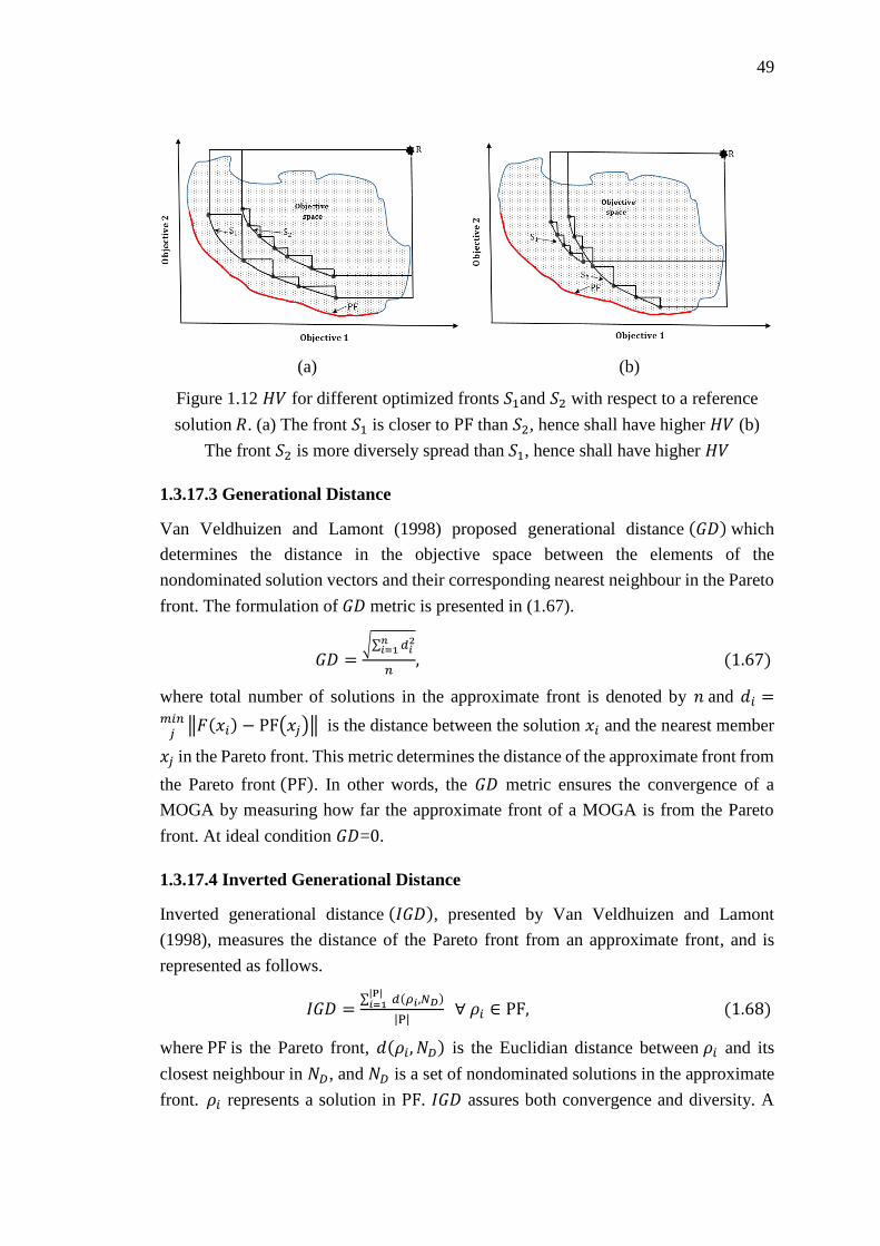
49

(a) (b)

Figure 1.12 𝐻𝑉 for different optimized fronts 𝑆1and 𝑆2 with respect to a reference

solution 𝑅. (a) The front 𝑆1 is closer to PF than 𝑆2, hence shall have higher 𝐻𝑉 (b)

The front 𝑆2 is more diversely spread than 𝑆1, hence shall have higher 𝐻𝑉

1.3.17.3 Generational Distance

Van Veldhuizen and Lamont (1998) proposed generational distance (𝐺𝐷) which

determines the distance in the objective space between the elements of the

nondominated solution vectors and their corresponding nearest neighbour in the Pareto

front. The formulation of 𝐺𝐷 metric is presented in (1.67).

𝐺𝐷 =√∑ 𝑑𝑖

2𝑛𝑖=1

𝑛, (1.67)

where total number of solutions in the approximate front is denoted by 𝑛 and 𝑑𝑖 =𝑚𝑖𝑛𝑗‖𝐹(𝑥𝑖) − PF(𝑥𝑗)‖ is the distance between the solution 𝑥𝑖 and the nearest member

𝑥𝑗 in the Pareto front. This metric determines the distance of the approximate front from

the Pareto front (PF). In other words, the 𝐺𝐷 metric ensures the convergence of a

MOGA by measuring how far the approximate front of a MOGA is from the Pareto

front. At ideal condition 𝐺𝐷=0.

1.3.17.4 Inverted Generational Distance

Inverted generational distance (𝐼𝐺𝐷), presented by Van Veldhuizen and Lamont

(1998), measures the distance of the Pareto front from an approximate front, and is

represented as follows.

𝐼𝐺𝐷 =∑ 𝑑(𝜌𝑖,𝑁𝐷)|P|𝑖=1

|P| ∀ 𝜌𝑖 ∈ PF, (1.68)

where PF is the Pareto front, 𝑑(𝜌𝑖, 𝑁𝐷) is the Euclidian distance between 𝜌𝑖 and its

closest neighbour in 𝑁𝐷, and 𝑁𝐷 is a set of nondominated solutions in the approximate

front. 𝜌𝑖 represents a solution in PF. 𝐼𝐺𝐷 assures both convergence and diversity. A

50

lower value of this metric can only be achieved if the solution set 𝑁𝐷 is close to PF and

nearly covers the spectrum of PF. Therefore, a smaller value of 𝐼𝐺𝐷 is always preferred.

1.4 Scope of the Thesis

In this thesis, we have presented some network optimization problems under various

uncertain environments including type-2 fuzzy, rough, rough fuzzy, random fuzzy and

uncertainty theory. The thesis is composed of seven chapters, among which the main

contribution of the thesis can be observed from Chapter 2 to Chapter 6. These five

chapters are further categorized into two parts, Part-I and Part-II. Part-I consists of

chapters 2 and 3, which deal with uncertain single objective optimization problems.

Whereas, Part-II comprises of chapters 4, 5 and 6, which address uncertain multi-

objective optimization problems. The chapters, presented in the thesis, are discussed

below in brief.

1.4.1 Introduction

In this chapter, we have presented a survey on the studies performed on four different

network optimization problems including transportation problem, shortest path

problem, minimum spanning tree problem and maximum flow problem, and their

variants under different uncertain paradigms. Moreover, some preliminary concepts,

definitions, theorems and methodologies pertinent to the thesis are also provided in this

chapter.

1.4.2 Linear Programming Model with Interval Type-2 Fuzzy Parameters and

its Application to some Network Problems

In this chapter, we propose a chance-constrained model to solve constrained linear

programming model with interval type-2 fuzzy parameters. It is developed using

credibility measure of interval type-2 fuzzy variable. The proposed method is applied

to three network optimization problems: (a) solid transportation problem, (b) shortest

path problem and (c) minimum spanning tree problem. In the solid transportation

problem, the parameters corresponding to the availability at sources, demands at

destinations and capacities of the conveyances are considered as trapezoidal interval

type-2 fuzzy variables (TrIT2FV). For the shortest path and minimum spanning tree

problems, the edge weights of the network are considered as TrIT2FVs. Numerical

examples of those problems are provided to illustrate the proposed method.

1.4.3 Genetic Algorithm with Varying Population for Random Fuzzy

Maximum Flow Problem

In this chapter, we have investigated the uncertain maximum flow problem (MFP) of a

network whose capacities are random fuzzy variables. We have developed the EVM

and CCM for MFP under random fuzzy environment, and formulate their crisp

51

equivalent models. To solve these models, we have proposed a varying population

genetic algorithm with indeterminate crossover (VPGAwIC). In VPGAwIC, selection

of a chromosome depends on its lifetime. For this purpose, we have proposed an

improved lifetime allocation strategy (iLAS). The ages of the chromosomes are defined

linguistically as Young, Middle and Old, which follow the linear and zigzag uncertainty

distributions (B. Liu 2007). The crossover probability is considered as indeterminate

and it depends on the ages of the parents. The crossover probability is defined by an

uncertain rule base. The number of offspring, generated from a population of parents,

is determined by reproduction ratio (Z. Michalewicz 1992), which is assumed to be

fixed. The population is updated in two ways. Firstly, all the chromosomes with ages

greater than their lifetimes are discarded from the population. Secondly, the offspring

are combined with their parents for the next generation. The performance of the

proposed VPGAwIC on MFP has been compared with that of the genetic algorithm

developed by Gen et al. (2008).

1.4.4 Multi-criteria Shortest Path Problem on Rough Graph

Shortest path problem (SPP) in real-world applications has to deal with multiple

criteria/objectives. This chapter is intended to solve a multi-criteria shortest path

problem (MSPP) of a weighted connected directed network (WCDN), where edge

weights are represented by rough variable. We have proposed two different approaches

to determine the optimum path(s) of MSPP. In the first approach, the rough variable

has been incorporated in the Dijkstra’s algorithm, which is named as modified rough

Dijkstra’s (MRD) algorithm. The second approach deals with modelling MSPP using

rough chance-constrained programming technique which is eventually solved by two

different methods: the goal attainment method and NSGA-II. The proposed

methodologies are numerically illustrated for a multi-criteria weighted connected

directed network (WCDN) and the simulated results are analyzed using large instances

of WCDN to show the efficiency of the proposed algorithms.

1.4.5 Uncertain Multi-objective Multi-item Fixed Charge Solid Transportation

Problem with Budget Constraint

Modelling real-world applications requires data as input parameter which represent

information represented in the state of indeterminacy. In this chapter, we have presented

an uncertain multi-objective multi-item fixed charge solid transportation problem with

budget constraint (UMMFSTPwB) at each destination. In the proposed model we have

optimized two objectives: (i) maximization of profit and (ii) minimization of time. In

the proposed UMMFSTPwB, it is considered that items are purchased at different

sources with different prices, and accordingly transported to different destinations using

different types of vehicles having different capacities. The items are sold to the

customers at different selling prices. Here, unit transportation costs, fixed charges,

52

transportation times, supplies at origins, demands at destinations, conveyance

capacities and budgets at destinations are assumed to be uncertain variables. For

UMMFSTPwB, we develop three uncertain programming models: (i) expected value

model (EVM) (ii) chance-constrained model (CCM) and (iii) dependent chance-

constrained model (DCCM). These models are formulated under the framework of

uncertainty theory. Finally, the equivalent deterministic models are formulated which

are solved using three methods: (i) linear weighted method, (ii) global criterion method

and (iii) fuzzy programming method. Suitable numerical examples have been used to

illustrate each of the models.

1.4.6 Multi-objective Rough Fuzzy Quadratic Minimum Spanning Tree

Problem

A quadratic minimum spanning tree problem determines a minimum spanning tree of

a network whose edges are associated with linear and quadratic weights. Linear weights

represent the edge costs, whereas the quadratic weights are the interaction costs

between a pair of edges of the graph. In this study, a bi-objective rough fuzzy quadratic

minimum spanning tree problem (b-RFQMSTP) has been proposed for a connected

graph, where the linear and the quadratic weights are represented by rough fuzzy

variable. The proposed model is formulated by using rough fuzzy chance-constrained

programming technique. Subsequently, three related theorems are also proposed for the

crisp transformation of the proposed model. The crisp equivalent models are solved by

a classical multi-objective solution technique, the epsilon-constraint method and two

multi-objective evolutionary algorithms: (i) NSGA-II and (ii) MOCHC. A numerical

example is provided to illustrate the proposed model when solved by different

methodologies. A sensitivity analysis of the example is also performed at different

confidence levels. The performance of NSGA-II and MOCHC are analyzed on five

randomly generated instances of the proposed model. Finally, a numerical illustration

of an application of the proposed model is also presented in this study.

1.4.7 Conclusion and Future Scope

In this chapter, we summarize the overall contribution of our studies and their possible

future extensions.

53

Part-I

Uncertain Single Objective

Optimization Problems

Chapter 2

Chapter 3

USER

Text Box

54

User

Text Box

55

Chapter 2

Linear Programming Model with

Interval Type-2 Fuzzy Parameters and

its Application to some Network

Problems

User

Text Box

56

User

Text Box

57

Chapter 2

Linear Programming Model with Interval

Type-2 Fuzzy Parameters and its Application

to some Network Problems

2.1 Introduction

In practice, decision making is a problem-solving activity, which is used to identify and

select alternatives based on the information and preferences of the decision makers

(DMs). Making a decision implies that there exist alternative solutions of the given

problem and we identify not only as many alternatives as possible but also choose the

one that best fits our goals, objectives and preferred values (R. Harris 1998).

Uncertainties involved in many decision making problems, in real-life can be broadly

classified into two types: (i) probabilistic and (ii) non-probabilistic. If there is enough

historical evidence, then probability theory is the only legitimate approach to deal with

uncertainty. Conversely, if there is a lack of historical evidence, then we have no option

but to invite some domain experts to evaluate the belief degree of the occurrence of an

event. Representation of uncertainty by evaluating the belief degrees of domain experts

is non-probabilistic. In this regard, type-1 fuzzy set (T1FS) is one of the widely used

and acceptable tool to deal with non-probabilistic uncertainty. Non-probabilistic

uncertainty usually occur due to the existence of uncertainties like scarcity of

information, multiple sources of available data, different perceptions of a concept

provided by multiple experts/decision makers and linguistic information. However, it

may not always be convenient to represent such imprecise information with the exact

membership function of T1FS. In that case, type-2 fuzzy set (T2FS) becomes a useful

tool which provides additional degrees of freedom for modelling uncertainties

compared to T1FS.

T2FS are the fuzzy sets with fuzzy membership functions proposed by L.A. Zadeh

(1975a, b) and developed by Mizumoto and Tanaka (1981), and Mandel and John

(2002, 2006). Motivated by the studies of those authors, Liu and Liu (2010) defined

type-2 fuzzy variable (T2FV), as a function from the fuzzy possibility space to the set

of real numbers. Recently, type-2 fuzzy set has attracted much attention and is applied

in various fields, such as data employment analysis (Qin et al. 2011), neural networks

(Aliev et al. 2011; Enke and Mehdiyev 2013), portfolio selection problem (Wu and Liu

User

Text Box

58

2012), multi-criteria group decision making (T.-Y. Chen 2013), transportation problem

(Liu et al. 2014a; Kundu et al. 2014a; Pramanik et al. 2015b), etc. However, due to the

three-dimensional nature of T2FS, the computational overhead involved in the

operations of T2FS, is very high. In this case, interval type-2 fuzzy sets (IT2FS)

(Mendel et al. 2006; Wu and Mendel 2007) is widely used. IT2FS is a special case of

general T2FS and computationally less complex. As an example of IT2FS, let us

consider the travelling cost between two cities is “around $ 80 − $ 100”. For such an

interval, the point values may not be equipossible or are equally important. Therefore,

it can be difficult to determine the exact membership value of each point in the range

of the travelling cost. To deal with such non-equipossible data, IT2FS can be considered

as an alternative.

Many real-life decision making problems in network optimization involve parameters

which are characteristically imprecise or uncertain. Under such circumstances, several

improved theories like probability theory, fuzzy set theory, rough set theory and

uncertainty theory are used to tackle imprecision. However, in this chapter, we have

confined our discussion, to the studies of three network optimization problem: (i) STP,

(ii) SPP and (iii) MSTP under fuzzy set theory (T1FS or T2FS). Considering fuzzy

environment, several studies can be observed in the literature on transportation problem

(TP) (Ammar and Youness 2005; Jiménez and Verdegay 1999; Kaur and Kumar 2012;

Peidro and Vasant 2011; Ojha et al. 2009), shortest path problem (SPP) (Okada and

Gen 1994; Keshavarz and Khorram 2009; Deng et al. 2012) and minimum spanning

tree problem (MSTP) (Janiak and Kasperski 2008; De Almeida et al. 2005a, b). In this

context, chance-constrained model (CCM) is considered as one of the important

approaches while formulating uncertain network problems. Under fuzzy environment,

CCM is first proposed by Liu and Iwamura (1998). Thereafter, the application of CCM

is observed in fuzzy TP (Yang and Liu 2007; Kundu et al. 2014a; Pramanik et al. 2015a,

c), fuzzy SPP (Ji et al. 2007; Dursun and Bozdağ 2014) and fuzzy MSTP (Itoh and Ishii

1996; Gao and Lu 2005; Zhou et al. 2013, 2016a). All these studies, mentioned above

are done by considering type-1 fuzzy parameters. However, under type-2 fuzzy

environment, relatively few research works have been done for transportation problem,

shortest path problem and minimum spanning tree problem. Considering TP, Kundu et

al. (2014a) first solved the fixed charge transportation problem (FTP) with generalized

triangular and trapezoidal type-2 fuzzy parameters. Consequently, Pramanik et al.

(2015b) addressed FTP in a two-stage supply chain network with generalized Gaussian

type-2 fuzzy parameters. Under interval type-2 fuzzy environment, Figueroa-García

and Hernández (2014) first considered a transportation problem with interval type-2

fuzzy supplies and demands. Subsequently, Sinha et al. (2016) solved an expected value

model (EVM) of profit maximization and time minimization solid transportation

problem (STP) with interval type-2 fuzzy variables. For SPP, Anusuya and Sathya

(2014) first solved the shortest path problem by considering edge weight as discrete

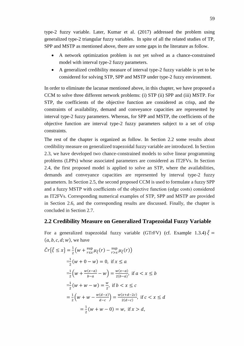
59

type-2 fuzzy variable. Later, Kumar et al. (2017) addressed the problem using

generalized type-2 triangular fuzzy variables. In spite of all the related studies of TP,

SPP and MSTP as mentioned above, there are some gaps in the literature as follow.

A network optimization problem is not yet solved as a chance-constrained

model with interval type-2 fuzzy parameters.

A generalized credibility measure of interval type-2 fuzzy variable is yet to be

considered for solving STP, SPP and MSTP under type-2 fuzzy environment.

In order to eliminate the lacunae mentioned above, in this chapter, we have proposed a

CCM to solve three different network problems: (i) STP (ii) SPP and (iii) MSTP. For

STP, the coefficients of the objective function are considered as crisp, and the

constraints of availability, demand and conveyance capacities are represented by

interval type-2 fuzzy parameters. Whereas, for SPP and MSTP, the coefficients of the

objective function are interval type-2 fuzzy parameters subject to a set of crisp

constraints.

The rest of the chapter is organized as follow. In Section 2.2 some results about

credibility measure on generalized trapezoidal fuzzy variable are introduced. In Section

2.3, we have developed two chance-constrained models to solve linear programming

problems (LPPs) whose associated parameters are considered as IT2FVs. In Section

2.4, the first proposed model is applied to solve an STP, where the availabilities,

demands and conveyance capacities are represented by interval type-2 fuzzy

parameters. In Section 2.5, the second proposed CCM is used to formulate a fuzzy SPP

and a fuzzy MSTP with coefficients of the objective function (edge costs) considered

as IT2FVs. Corresponding numerical examples of STP, SPP and MSTP are provided

in Section 2.6, and the corresponding results are discussed. Finally, the chapter is

concluded in Section 2.7.

2.2 Credibility Measure on Generalized Trapezoidal Fuzzy Variable

For a generalized trapezoidal fuzzy variable (GTrFV) (cf. Example 1.3.4) 𝜉 =

(𝑎, 𝑏, 𝑐, 𝑑; 𝑤), we have

��𝑟{𝜉 ≤ 𝑥} =1

2(𝑤 + sup

𝑟≤𝑥𝜇��(𝑟) −

sup𝑟>𝑥

𝜇��(𝑟))

=1

2(𝑤 + 0 − 𝑤) = 0, if 𝑥 ≤ 𝑎

=1

2(𝑤 +

𝑤(𝑥−𝑎)

𝑏−𝑎− 𝑤) =

𝑤(𝑥−𝑎)

2(𝑏−𝑎), if 𝑎 < 𝑥 ≤ 𝑏

=1

2(𝑤 + 𝑤 −𝑤) =

𝑤

2, if 𝑏 < 𝑥 ≤ 𝑐

=1

2(𝑤 + 𝑤 −

𝑤(𝑑−𝑥)

𝑑−𝑐) =

𝑤(𝑥+𝑑−2𝑐)

2(𝑑−𝑐), if 𝑐 < 𝑥 ≤ 𝑑

=1

2(𝑤 + 𝑤 − 0) = 𝑤, if 𝑥 > 𝑑,

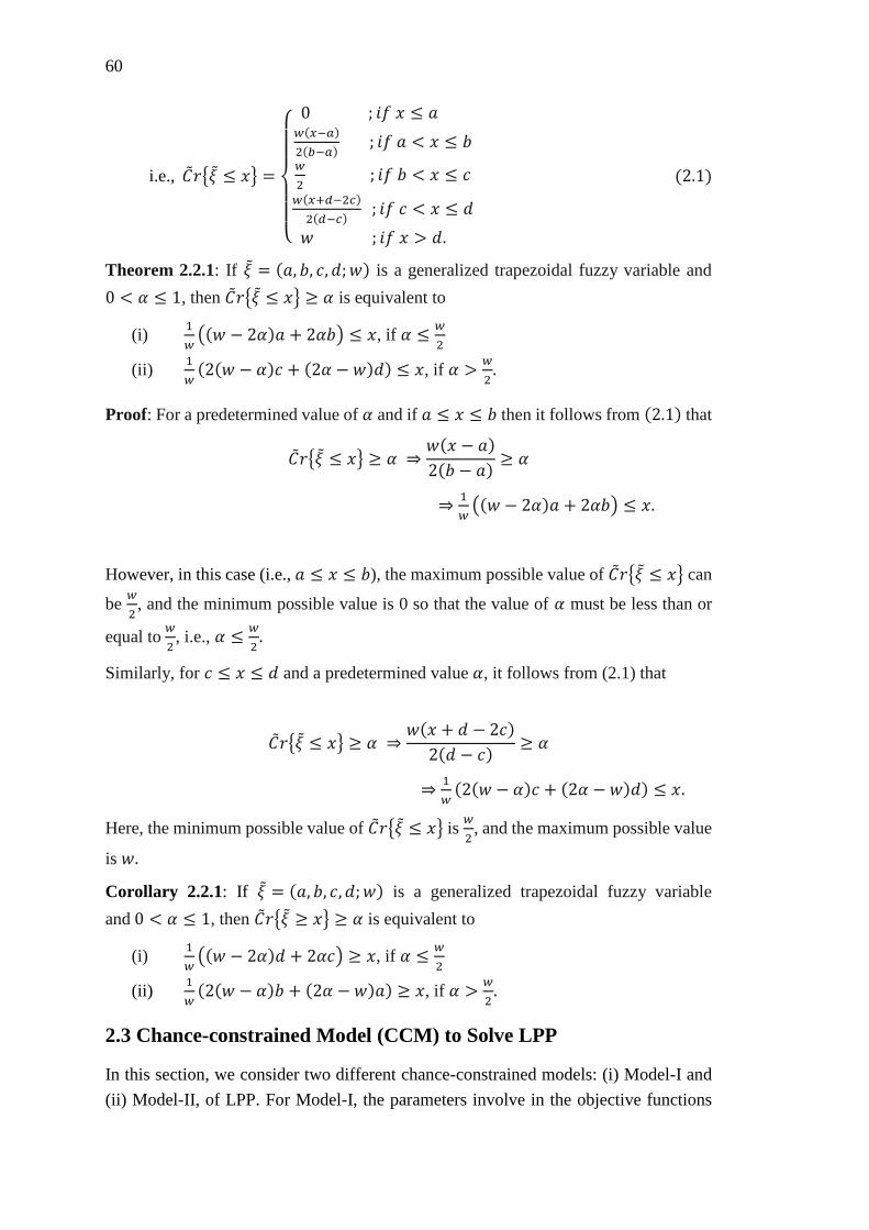
60

i.e., ��𝑟{𝜉 ≤ 𝑥} =

{

0 ; 𝑖𝑓 𝑥 ≤ 𝑎 𝑤(𝑥−𝑎)

2(𝑏−𝑎) ; 𝑖𝑓 𝑎 < 𝑥 ≤ 𝑏

𝑤

2 ; 𝑖𝑓 𝑏 < 𝑥 ≤ 𝑐

𝑤(𝑥+𝑑−2𝑐)

2(𝑑−𝑐) ; 𝑖𝑓 𝑐 < 𝑥 ≤ 𝑑

𝑤 ; 𝑖𝑓 𝑥 > 𝑑.

(2.1)

Theorem 2.2.1: If 𝜉 = (𝑎, 𝑏, 𝑐, 𝑑; 𝑤) is a generalized trapezoidal fuzzy variable and

0 < 𝛼 ≤ 1, then ��𝑟{𝜉 ≤ 𝑥} ≥ 𝛼 is equivalent to

(i) 1

𝑤((𝑤 − 2𝛼)𝑎 + 2𝛼𝑏) ≤ 𝑥, if 𝛼 ≤

𝑤

2

(ii) 1

𝑤(2(𝑤 − 𝛼)𝑐 + (2𝛼 − 𝑤)𝑑) ≤ 𝑥, if 𝛼 >

𝑤

2.

Proof: For a predetermined value of 𝛼 and if 𝑎 ≤ 𝑥 ≤ 𝑏 then it follows from (2.1) that

��𝑟{𝜉 ≤ 𝑥} ≥ 𝛼 ⇒𝑤(𝑥 − 𝑎)

2(𝑏 − 𝑎)≥ 𝛼

⇒1

𝑤((𝑤 − 2𝛼)𝑎 + 2𝛼𝑏) ≤ 𝑥.

However, in this case (i.e., 𝑎 ≤ 𝑥 ≤ 𝑏), the maximum possible value of ��𝑟{𝜉 ≤ 𝑥} can

be 𝑤

2, and the minimum possible value is 0 so that the value of 𝛼 must be less than or

equal to 𝑤

2, i.e., 𝛼 ≤

𝑤

2.

Similarly, for 𝑐 ≤ 𝑥 ≤ 𝑑 and a predetermined value 𝛼, it follows from (2.1) that

��𝑟{𝜉 ≤ 𝑥} ≥ 𝛼 ⇒𝑤(𝑥 + 𝑑 − 2𝑐)

2(𝑑 − 𝑐)≥ 𝛼

⇒1

𝑤(2(𝑤 − 𝛼)𝑐 + (2𝛼 − 𝑤)𝑑) ≤ 𝑥.

Here, the minimum possible value of ��𝑟{𝜉 ≤ 𝑥} is 𝑤

2, and the maximum possible value

is 𝑤.

Corollary 2.2.1: If 𝜉 = (𝑎, 𝑏, 𝑐, 𝑑; 𝑤) is a generalized trapezoidal fuzzy variable

and 0 < 𝛼 ≤ 1, then ��𝑟{𝜉 ≥ 𝑥} ≥ 𝛼 is equivalent to

(i) 1

𝑤((𝑤 − 2𝛼)𝑑 + 2𝛼𝑐) ≥ 𝑥, if 𝛼 ≤

𝑤

2

(ii) 1

𝑤(2(𝑤 − 𝛼)𝑏 + (2𝛼 − 𝑤)𝑎) ≥ 𝑥, if 𝛼 >

𝑤

2.

2.3 Chance-constrained Model (CCM) to Solve LPP

In this section, we consider two different chance-constrained models: (i) Model-I and

(ii) Model-II, of LPP. For Model-I, the parameters involve in the objective functions

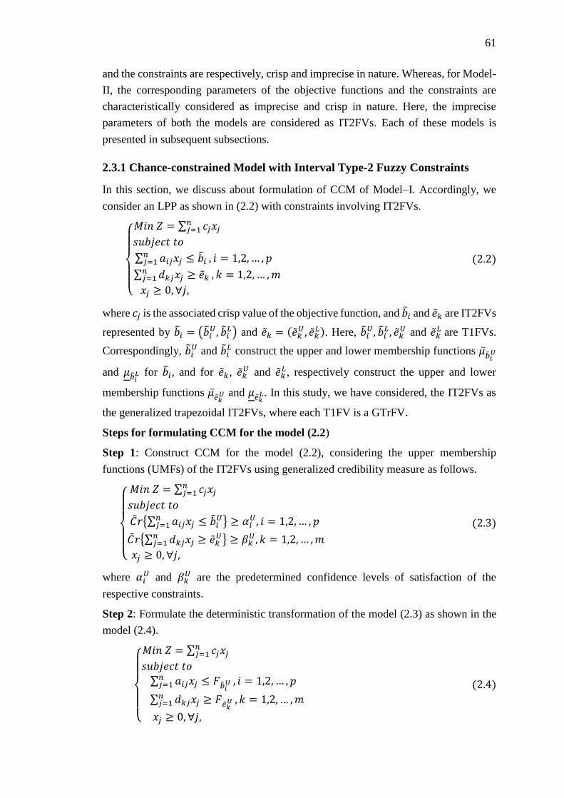
61

and the constraints are respectively, crisp and imprecise in nature. Whereas, for Model-

II, the corresponding parameters of the objective functions and the constraints are

characteristically considered as imprecise and crisp in nature. Here, the imprecise

parameters of both the models are considered as IT2FVs. Each of these models is

presented in subsequent subsections.

2.3.1 Chance-constrained Model with Interval Type-2 Fuzzy Constraints

In this section, we discuss about formulation of CCM of Model–I. Accordingly, we

consider an LPP as shown in (2.2) with constraints involving IT2FVs.

{

𝑀𝑖𝑛 𝑍 = ∑ 𝑐𝑗𝑥𝑗

𝑛𝑗=1


∑ 𝑎𝑖𝑗𝑥𝑗 ≤ ��𝑖𝑛𝑗=1 , 𝑖 = 1,2, … , 𝑝

∑ 𝑑𝑘𝑗𝑥𝑗 ≥ ��𝑘𝑛𝑗=1 , 𝑘 = 1,2, … ,𝑚

𝑥𝑗 ≥ 0, ∀𝑗,

(2.2)

where 𝑐𝑗 is the associated crisp value of the objective function, and ��𝑖 and ��𝑘 are IT2FVs

represented by ��𝑖 = (��𝑖𝑈, ��𝑖

𝐿) and ��𝑘 = (��𝑘𝑈, ��𝑘

𝐿). Here, ��𝑖𝑈, ��𝑖

𝐿 , ��𝑘𝑈 and ��𝑘

𝐿 are T1FVs.

Correspondingly, ��𝑖𝑈 and ��𝑖

𝐿 construct the upper and lower membership functions ��𝑖𝑈

and 𝜇��𝑖𝐿 for ��𝑖, and for ��𝑘, ��𝑘

𝑈 and ��𝑘𝐿, respectively construct the upper and lower

membership functions ��𝑘𝑈 and 𝜇��𝑘

𝐿. In this study, we have considered, the IT2FVs as

the generalized trapezoidal IT2FVs, where each T1FV is a GTrFV.

Steps for formulating CCM for the model (2.2)

Step 1: Construct CCM for the model (2.2), considering the upper membership

functions (UMFs) of the IT2FVs using generalized credibility measure as follows.

{


𝑛𝑗=1


��𝑟{∑ 𝑎𝑖𝑗𝑥𝑗 ≤ ��𝑖𝑈𝑛

𝑗=1 } ≥ 𝛼𝑖𝑈, 𝑖 = 1,2, … , 𝑝

��𝑟{∑ 𝑑𝑘𝑗𝑥𝑗 ≥ ��𝑘𝑈𝑛

𝑗=1 } ≥ 𝛽𝑘𝑈, 𝑘 = 1,2, … ,𝑚

𝑥𝑗 ≥ 0, ∀𝑗,

(2.3)

where 𝛼𝑖𝑈 and 𝛽𝑘

𝑈 are the predetermined confidence levels of satisfaction of the

respective constraints.

Step 2: Formulate the deterministic transformation of the model (2.3) as shown in the

model (2.4).

{


𝑛𝑗=1

𝑠𝑢𝑏𝑗𝑒𝑐𝑡 𝑡𝑜 ∑ 𝑎𝑖𝑗𝑥𝑗 ≤ 𝐹��𝑖

𝑈𝑛𝑗=1 , 𝑖 = 1,2, … , 𝑝

∑ 𝑑𝑘𝑗𝑥𝑗 ≥ 𝐹��𝑘𝑈

𝑛𝑗=1 , 𝑘 = 1,2, … ,𝑚

𝑥𝑗 ≥ 0, ∀𝑗,

(2.4)

62

where the deterministic transformations of the two constraints of model (2.4) are

obtained by following Corollary 2.2.1 and Theorem 2.2.1, respectively. 𝐹��𝑖𝑈 and 𝐹��𝑘

𝑈

are the resulting defuzzified values corresponding to the GTrFVs ��𝑖𝑈 and ��𝑘

𝑈.

Step 3: Solve model (2.4) and suppose after solving we have 𝑀𝑖𝑛 𝑍 = 𝑍′.

Step 4: Construct CCM for the model (2.2), considering the lower membership

functions (LMFs) of the IT2FVs using generalized credibility measure as follows.

{


𝑛𝑗=1


��𝑟{∑ 𝑎𝑖𝑗𝑥𝑗 ≤ ��𝑖𝐿𝑛

𝑗=1 } ≥ 𝛼𝑖𝐿 , 𝑖 = 1,2, … , 𝑝

��𝑟{∑ 𝑑𝑘𝑗𝑥𝑗 ≥ ��𝑘𝐿𝑛

𝑗=1 } ≥ 𝛽𝑘𝐿 , 𝑘 = 1,2, … ,𝑚

𝑥𝑗 ≥ 0, ∀𝑗,

(2.5)

where 𝛼𝑖𝐿 and 𝛽𝑘

𝐿 are the predetermined confidence levels of satisfaction of the

respective constraints.

Step 5: Formulate the deterministic transformation of the model (2.5) as follows.

{


𝑛𝑗=1

𝑠𝑢𝑏𝑗𝑒𝑐𝑡 𝑡𝑜 ∑ 𝑎𝑖𝑗𝑥𝑗 ≤ 𝐹��𝑖

𝐿𝑛𝑗=1 , 𝑖 = 1,2, … , 𝑝

∑ 𝑑𝑘𝑗𝑥𝑗 ≥ 𝐹��𝑘𝐿

𝑛𝑗=1 , 𝑘 = 1,2, … ,𝑚

𝑥𝑗 ≥ 0, ∀𝑗,

(2.6)

where the deterministic transformation of the two constraints of the model (2.6) are

obtained in the same way as mentioned in Step 2, and 𝐹��𝑖𝐿 and 𝐹��𝑘

𝐿 are respectively,

the resulting defuzzified values of ��𝑖𝐿 and ��𝑘

𝐿.

Step 6: Solve model (2.6) and suppose after solving we have 𝑀𝑖𝑛 𝑍 = 𝑍′′.

Step 7: Let us denote 𝑍𝑚𝑖𝑛 = 𝑀𝑖𝑛(𝑍′, 𝑍′′), 𝑍𝑚𝑎𝑥 = 𝑀𝑎𝑥(𝑍′, 𝑍′′),

𝐹��𝑖𝑚𝑖𝑛 = 𝑀𝑖𝑛 (𝐹��𝑖

𝑈 , 𝐹��𝑖𝐿), 𝐹��𝑖

𝑚𝑎𝑥 = 𝑀𝑎𝑥 (𝐹��𝑖𝑈 , 𝐹��𝑖

𝐿), 𝐹��𝑘𝑚𝑖𝑛 = 𝑀𝑖𝑛 (𝐹��𝑘

𝑈 , 𝐹��𝑘𝐿) and

𝐹��𝑘𝑚𝑎𝑥 = 𝑀𝑎𝑥 (𝐹��𝑘

𝑈 , 𝐹��𝑘𝐿). Here, in order to determine a compromise solution within the

interval [𝑍𝑚𝑖𝑛, 𝑍𝑚𝑎𝑥], we use fuzzy programming method (H.-J. Zimmermann 1978).

Accordingly, we determine the following membership function (for the minimization

problem).

𝜇(𝑍) = {

1 ; 𝑖𝑓 𝑍 ≤ 𝑍𝑚𝑖𝑛 𝑍𝑚𝑎𝑥−𝑍

𝑍𝑚𝑎𝑥−𝑍𝑚𝑖𝑛 ; 𝑖𝑓 𝑍𝑚𝑖𝑛 < 𝑍 < 𝑍𝑚𝑎𝑥

0 ; 𝑖𝑓 𝑍 ≥ 𝑍𝑚𝑎𝑥 .

Here, maximum 𝜇(𝑍) means a better solution for a minimization problem. Now to

obtain a compromise solution by ensuring the maximum possible satisfaction of the

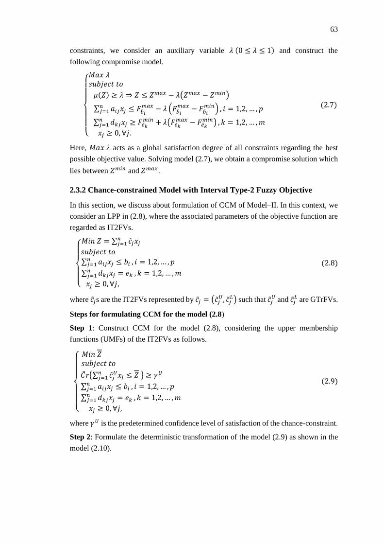
63

constraints, we consider an auxiliary variable 𝜆 (0 ≤ 𝜆 ≤ 1) and construct the

following compromise model.

{

𝑀𝑎𝑥 𝜆 𝑠𝑢𝑏𝑗𝑒𝑐𝑡 𝑡𝑜

𝜇(𝑍) ≥ 𝜆 ⇒ 𝑍 ≤ 𝑍𝑚𝑎𝑥 − 𝜆(𝑍𝑚𝑎𝑥 − 𝑍𝑚𝑖𝑛)

∑ 𝑎𝑖𝑗𝑥𝑗 ≤ 𝐹��𝑖𝑚𝑎𝑥 − 𝜆 (𝐹��𝑖

𝑚𝑎𝑥 − 𝐹��𝑖𝑚𝑖𝑛)𝑛

𝑗=1 , 𝑖 = 1,2, … , 𝑝

∑ 𝑑𝑘𝑗𝑥𝑗 ≥ 𝐹��𝑘𝑚𝑖𝑛 + 𝜆(𝐹��𝑘

𝑚𝑎𝑥 − 𝐹��𝑘𝑚𝑖𝑛)𝑛

𝑗=1 , 𝑘 = 1,2, … ,𝑚

𝑥𝑗 ≥ 0, ∀𝑗.

(2.7)

Here, 𝑀𝑎𝑥 𝜆 acts as a global satisfaction degree of all constraints regarding the best

possible objective value. Solving model (2.7), we obtain a compromise solution which

lies between 𝑍𝑚𝑖𝑛 and 𝑍𝑚𝑎𝑥.

2.3.2 Chance-constrained Model with Interval Type-2 Fuzzy Objective

In this section, we discuss about formulation of CCM of Model–II. In this context, we

consider an LPP in (2.8), where the associated parameters of the objective function are

regarded as IT2FVs.

{

𝑀𝑖𝑛 𝑍 = ∑ ��𝑗𝑥𝑗

𝑛𝑗=1

𝑠𝑢𝑏𝑗𝑒𝑐𝑡 𝑡𝑜 ∑ 𝑎𝑖𝑗𝑥𝑗 ≤ 𝑏𝑖𝑛𝑗=1 , 𝑖 = 1,2, … , 𝑝

∑ 𝑑𝑘𝑗𝑥𝑗 = 𝑒𝑘𝑛𝑗=1 , 𝑘 = 1,2, … ,𝑚

𝑥𝑗 ≥ 0, ∀𝑗,

(2.8)

where ��𝑗s are the IT2FVs represented by ��𝑗 = (��𝑗𝑈, ��𝑗

𝐿) such that ��𝑗𝑈 and ��𝑗

𝐿 are GTrFVs.

Steps for formulating CCM for the model (2.8)

Step 1: Construct CCM for the model (2.8), considering the upper membership

functions (UMFs) of the IT2FVs as follows.

{

𝑀𝑖𝑛 𝑍 𝑠𝑢𝑏𝑗𝑒𝑐𝑡 𝑡𝑜

��𝑟{∑ ��𝑗𝑈𝑥𝑗

𝑛𝑗=1 ≤ 𝑍 } ≥ 𝛾𝑈

∑ 𝑎𝑖𝑗𝑥𝑗 ≤ 𝑏𝑖𝑛𝑗=1 , 𝑖 = 1,2, … , 𝑝

∑ 𝑑𝑘𝑗𝑥𝑗 = 𝑒𝑘𝑛𝑗=1 , 𝑘 = 1,2, … ,𝑚

𝑥𝑗 ≥ 0, ∀𝑗,

(2.9)

where 𝛾𝑈 is the predetermined confidence level of satisfaction of the chance-constraint.


model (2.10).

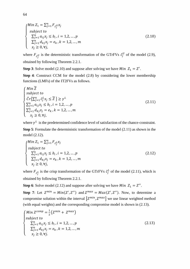
64

{

𝑀𝑖𝑛 𝑍1 = ∑ 𝐹𝑐��

𝑈𝑥𝑗𝑛𝑗=1


∑ 𝑑𝑘𝑗𝑥𝑗 = 𝑒𝑘𝑛𝑗=1 , 𝑘 = 1,2, … ,𝑚

𝑥𝑗 ≥ 0, ∀𝑗,

(2.10)

where 𝐹𝑐��𝑈 is the deterministic transformation of the GTrFVs ��𝑗

𝑈 of the model (2.9),

obtained by following Theorem 2.2.1.

Step 3: Solve model (2.10) and suppose after solving we have 𝑀𝑖𝑛 𝑍1 = 𝑍′.

Step 4: Construct CCM for the model (2.8) by considering the lower membership

functions (LMFs) of the IT2FVs as follows.

{


��𝑟{∑ ��𝑗𝐿𝑥𝑗

𝑛𝑗=1 ≤ 𝑍 } ≥ 𝛾𝐿

∑ 𝑎𝑖𝑗𝑥𝑗 ≤ 𝑏𝑖𝑛𝑗=1 , 𝑖 = 1,2, … , 𝑝

∑ 𝑑𝑘𝑗𝑥𝑗 = 𝑒𝑘𝑛𝑗=1 , 𝑘 = 1,2, … ,𝑚

𝑥𝑗 ≥ 0, ∀𝑗,

(2.11)

where 𝛾𝐿 is the predetermined confidence level of satisfaction of the chance-constraint.


model (2.12).

{

𝑀𝑖𝑛 𝑍1 = ∑ 𝐹𝑐��

𝐿𝑥𝑗𝑛𝑗=1


∑ 𝑑𝑘𝑗𝑥𝑗 = 𝑒𝑘𝑛𝑗=1 , 𝑘 = 1,2, … ,𝑚

𝑥𝑗 ≥ 0, ∀𝑗,

(2.12)

where 𝐹𝑐��𝐿 is the crisp transformation of the GTrFVs ��𝑗

𝐿 of the model (2.11), which is

obtained by following Theorem 2.2.1.

Step 6: Solve model (2.12) and suppose after solving we have 𝑀𝑖𝑛 𝑍1 = 𝑍′′.

Step 7: Let 𝑍𝑚𝑖𝑛 = 𝑀𝑖𝑛(𝑍′, 𝑍′′) and 𝑍𝑚𝑎𝑥 = 𝑀𝑎𝑥(𝑍′, 𝑍′′). Now, to determine a

compromise solution within the interval [𝑍𝑚𝑖𝑛, 𝑍𝑚𝑎𝑥] we use linear weighted method

(with equal weights) and the corresponding compromise model is shown in (2.13).

{

𝑀𝑖𝑛 𝑍

𝑐𝑜𝑚𝑝 =1

2(𝑍𝑚𝑖𝑛 + 𝑍𝑚𝑎𝑥)


∑ 𝑑𝑘𝑗𝑥𝑗 = 𝑒𝑘𝑛𝑗=1 , 𝑘 = 1,2, … ,𝑚

𝑥𝑗 ≥ 0, ∀𝑗.

(2.13)

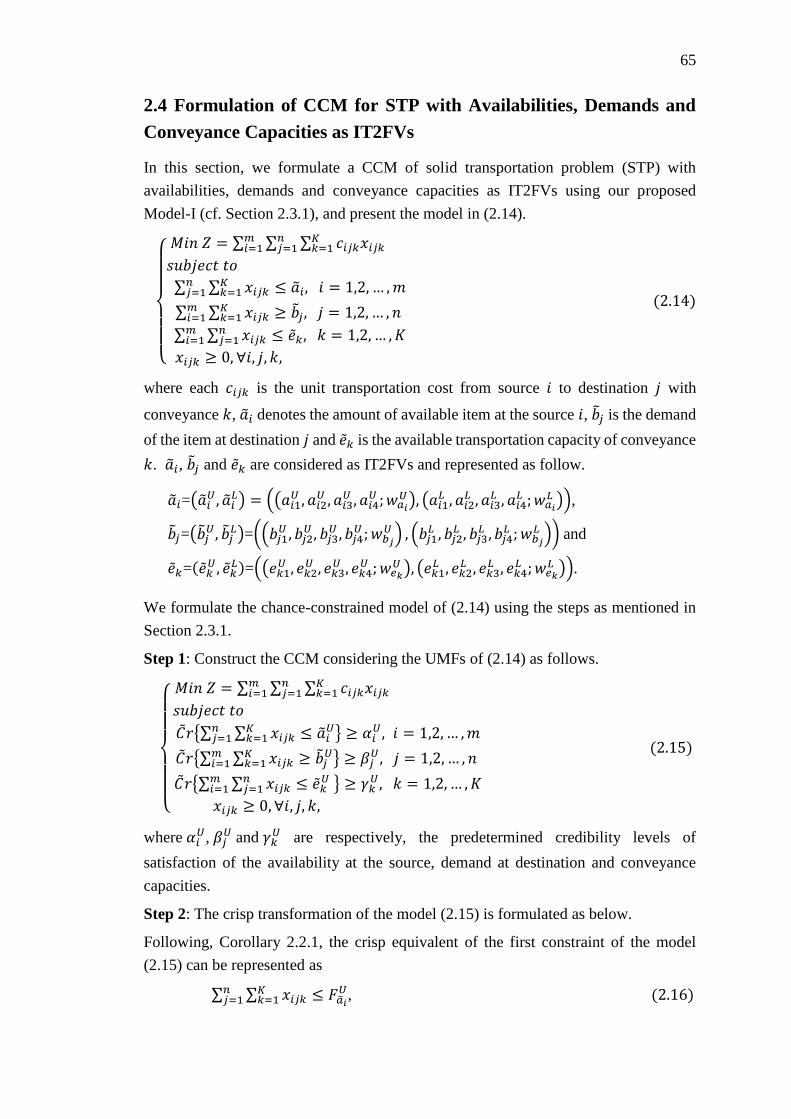
65

2.4 Formulation of CCM for STP with Availabilities, Demands and

Conveyance Capacities as IT2FVs

In this section, we formulate a CCM of solid transportation problem (STP) with

availabilities, demands and conveyance capacities as IT2FVs using our proposed

Model-I (cf. Section 2.3.1), and present the model in (2.14).

{

𝑀𝑖𝑛 𝑍 = ∑ ∑ ∑ 𝑐𝑖𝑗𝑘𝑥𝑖𝑗𝑘

𝐾𝑘=1

𝑛𝑗=1

𝑚𝑖=1


∑ ∑ 𝑥𝑖𝑗𝑘 ≤ ��𝑖, 𝑖 = 1,2, … ,𝑚𝐾𝑘=1

𝑛𝑗=1

∑ ∑ 𝑥𝑖𝑗𝑘 ≥ ��𝑗, 𝑗 = 1,2, … , 𝑛𝐾𝑘=1

𝑚𝑖=1

∑ ∑ 𝑥𝑖𝑗𝑘 ≤ ��𝑘, 𝑘 = 1,2, … , 𝐾𝑛𝑗=1

𝑚𝑖=1

𝑥𝑖𝑗𝑘 ≥ 0, ∀𝑖, 𝑗, 𝑘,

(2.14)

where each 𝑐𝑖𝑗𝑘 is the unit transportation cost from source 𝑖 to destination 𝑗 with

conveyance 𝑘, ��𝑖 denotes the amount of available item at the source 𝑖, ��𝑗 is the demand

of the item at destination 𝑗 and ��𝑘 is the available transportation capacity of conveyance

𝑘. ��𝑖, ��𝑗 and ��𝑘 are considered as IT2FVs and represented as follow.

��𝑖=(��𝑖𝑈, ��𝑖

𝐿) = ((𝑎𝑖1𝑈 , 𝑎𝑖2

𝑈 , 𝑎𝑖3𝑈 , 𝑎𝑖4

𝑈 ; 𝑤𝑎𝑖𝑈), (𝑎𝑖1

𝐿 , 𝑎𝑖2𝐿 , 𝑎𝑖3

𝐿 , 𝑎𝑖4𝐿 ; 𝑤𝑎𝑖

𝐿 )),

��𝑗=(��𝑗𝑈, ��𝑗

𝐿)=((𝑏𝑗1𝑈 , 𝑏𝑗2

𝑈 , 𝑏𝑗3𝑈 , 𝑏𝑗4

𝑈 ; 𝑤𝑏𝑗𝑈 ) , (𝑏𝑗1

𝐿 , 𝑏𝑗2𝐿 , 𝑏𝑗3

𝐿 , 𝑏𝑗4𝐿 ; 𝑤𝑏𝑗

𝐿 )) and

��𝑘=(��𝑘𝑈, ��𝑘

𝐿)=((𝑒𝑘1𝑈 , 𝑒𝑘2

𝑈 , 𝑒𝑘3𝑈 , 𝑒𝑘4

𝑈 ; 𝑤𝑒𝑘𝑈 ), (𝑒𝑘1

𝐿 , 𝑒𝑘2𝐿 , 𝑒𝑘3

𝐿 , 𝑒𝑘4𝐿 ; 𝑤𝑒𝑘

𝐿 )).

We formulate the chance-constrained model of (2.14) using the steps as mentioned in

Section 2.3.1.

Step 1: Construct the CCM considering the UMFs of (2.14) as follows.

{


𝐾𝑘=1

𝑛𝑗=1

𝑚𝑖=1


��𝑟{∑ ∑ 𝑥𝑖𝑗𝑘 ≤ ��𝑖𝑈𝐾

𝑘=1𝑛𝑗=1 } ≥ 𝛼𝑖

𝑈, 𝑖 = 1,2, … ,𝑚

��𝑟{∑ ∑ 𝑥𝑖𝑗𝑘 ≥ ��𝑗𝑈𝐾

𝑘=1𝑚𝑖=1 } ≥ 𝛽𝑗

𝑈, 𝑗 = 1,2, … , 𝑛

��𝑟{∑ ∑ 𝑥𝑖𝑗𝑘 ≤ ��𝑘𝑈𝑛

𝑗=1𝑚𝑖=1 } ≥ 𝛾𝑘

𝑈, 𝑘 = 1,2, … , 𝐾

𝑥𝑖𝑗𝑘 ≥ 0, ∀𝑖, 𝑗, 𝑘,

(2.15)

where 𝛼𝑖𝑈, 𝛽𝑗

𝑈 and 𝛾𝑘𝑈 are respectively, the predetermined credibility levels of

satisfaction of the availability at the source, demand at destination and conveyance

capacities.

Step 2: The crisp transformation of the model (2.15) is formulated as below.

Following, Corollary 2.2.1, the crisp equivalent of the first constraint of the model

(2.15) can be represented as

∑ ∑ 𝑥𝑖𝑗𝑘 ≤ 𝐹��𝑖𝑈𝐾

𝑘=1𝑛𝑗=1 , (2.16)

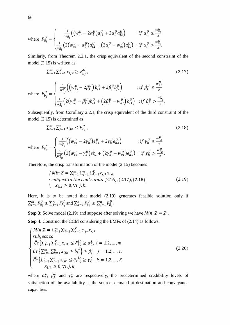
66

where 𝐹��𝑖𝑈 =

{

1

𝑤𝑎𝑖𝑈 ((𝑤𝑎𝑖

𝑈 − 2𝛼𝑖𝑈)𝑎𝑖4

𝑈 + 2𝛼𝑖𝑈𝑎𝑖3

𝑈 ) ; 𝑖𝑓 𝛼𝑖𝑈 ≤

𝑤𝑎𝑖𝑈

2

1

𝑤𝑎𝑖𝑈 (2(𝑤𝑎𝑖

𝑈 − 𝛼𝑖𝑈)𝑎𝑖2

𝑈 + (2𝛼𝑖𝑈 − 𝑤𝑎𝑖

𝑈)𝑎𝑖1𝑈 ) ; 𝑖𝑓 𝛼𝑖

𝑈 >𝑤𝑎𝑖𝑈

2.

Similarly, from Theorem 2.2.1, the crisp equivalent of the second constraint of the

model (2.15) is written as

∑ ∑ 𝑥𝑖𝑗𝑘 ≥ 𝐹��𝑗𝑈𝐾

𝑘=1𝑚𝑖=1 , (2.17)

where 𝐹��𝑗𝑈 =

{

1

𝑤𝑏𝑗𝑈 ((𝑤𝑏𝑗

𝑈 − 2𝛽𝑗𝑈) 𝑏𝑗1

𝑈 + 2𝛽𝑗𝑈𝑏𝑗2

𝑈) ; 𝑖𝑓 𝛽𝑗𝑈 ≤

𝑤𝑏𝑗𝑈

2

1

𝑤𝑎𝑖𝑈 (2(𝑤𝑏𝑖

𝑈 − 𝛽𝑗𝑈)𝑏𝑗3

𝑈 + (2𝛽𝑗𝑈 − 𝑤𝑏𝑗

𝑈 ) 𝑏𝑗4𝑈) ; 𝑖𝑓 𝛽𝑗

𝑈 >𝑤𝑏𝑗𝑈

2.

Subsequently, from Corollary 2.2.1, the crisp equivalent of the third constraint of the

model (2.15) is determined as

∑ ∑ 𝑥𝑖𝑗𝑘 ≤ 𝐹��𝑘𝑈𝑛

𝑗=1𝑚𝑖=1 , (2.18)

where 𝐹��𝑘𝑈 =

{

1

𝑤𝑒𝑘𝑈 ((𝑤𝑒𝑘

𝑈 − 2𝛾𝑘𝑈)𝑒𝑘4

𝑈 + 2𝛾𝑘𝑈𝑒𝑘3

𝑈 ) ; 𝑖𝑓 𝛾𝑘𝑈 ≤

𝑤𝑒𝑘𝑈

2

1

𝑤𝑒𝑘𝑈 (2(𝑤𝑒𝑘

𝑈 − 𝛾𝑘𝑈)𝑒𝑘2

𝑈 + (2𝛾𝑘𝑈 − 𝑤𝑒𝑘

𝑈 )𝑒𝑘1𝑈 ) ; 𝑖𝑓 𝛾𝑘

𝑈 >𝑤𝑒𝑘𝑈

2.

Therefore, the crisp transformation of the model (2.15) becomes

{

𝑀𝑖𝑛 𝑍 = ∑ ∑ ∑ 𝑐𝑖𝑗𝑘𝑥𝑖𝑗𝑘𝐾𝑘=1

𝑛𝑗=1

𝑚𝑖=1

𝑠𝑢𝑏𝑗𝑒𝑐𝑡 𝑡𝑜 𝑡ℎ𝑒 𝑐𝑜𝑛𝑡𝑟𝑎𝑖𝑛𝑡𝑠 (2.16), (2.17), (2.18)𝑥𝑖𝑗𝑘 ≥ 0, ∀𝑖, 𝑗, 𝑘.

(2.19)

Here, it is to be noted that model (2.19) generates feasible solution only if

∑ 𝐹��𝑖𝑈 ≥ ∑ 𝐹��𝑗

𝑈𝑛𝑗=1

𝑚𝑖=1 and ∑ 𝐹��𝑘

𝑈 ≥ ∑ 𝐹��𝑗𝑈𝑛

𝑗=1𝐾𝑘=1 .

Step 3: Solve model (2.19) and suppose after solving we have 𝑀𝑖𝑛 𝑍 = 𝑍′.

Step 4: Construct the CCM considering the LMFs of (2.14) as follows.

{


𝐾𝑘=1

𝑛𝑗=1

𝑚𝑖=1


��𝑟{∑ ∑ 𝑥𝑖𝑗𝑘 ≤ ��𝑖𝐿𝐾

𝑘=1𝑛𝑗=1 } ≥ 𝛼𝑖

𝐿 , 𝑖 = 1,2, … ,𝑚

��𝑟 {∑ ∑ 𝑥𝑖𝑗𝑘 ≥ ��𝑗𝐾𝑘=1

𝑚𝑖=1

𝐿} ≥ 𝛽𝑗

𝐿 , 𝑗 = 1,2, … , 𝑛

��𝑟{∑ ∑ 𝑥𝑖𝑗𝑘 ≤ ��𝑘𝑛𝑗=1

𝐿𝑚𝑖=1 } ≥ 𝛾𝑘

𝐿 , 𝑘 = 1,2, … , 𝐾

𝑥𝑖𝑗𝑘 ≥ 0, ∀𝑖, 𝑗, 𝑘,

(2.20)

where 𝛼𝑖𝐿, 𝛽𝑗

𝐿 and 𝛾𝑘𝐿 are respectively, the predetermined credibility levels of

satisfaction of the availability at the source, demand at destination and conveyance

capacities.

67

Step 5: The crisp transformation of model (2.20) is formulated below.

Similar to Step 2, following the Theorem 2.2.1 and Corollary 2.2.1, the crisp equivalent

of the first, second and third constraints of the model (2.20) are respectively, shown in

(2.21), (2.22) and (2.23).

∑ ∑ 𝑥𝑖𝑗𝑘 ≤ 𝐹��𝑖𝐿𝐾

𝑘=1𝑛𝑗=1 (2.21)

∑ ∑ 𝑥𝑖𝑗𝑘 ≥ 𝐹��𝑗𝐿𝐾

𝑘=1𝑚𝑖=1 (2.22)

∑ ∑ 𝑥𝑖𝑗𝑘 ≤ 𝐹��𝑘𝐿𝑛

𝑗=1𝑚𝑖=1 , (2.23)

where

𝐹��𝑖𝐿 =

{

1

𝑤𝑎𝑖𝐿((𝑤𝑎𝑖

𝐿 − 2𝛼𝑖𝐿)𝑎𝑖4

𝐿 + 2𝛼𝑖𝐿𝑎𝑖3

𝐿 ) ; 𝑖𝑓 𝛼𝑖𝐿 ≤

𝑤𝑎𝑖𝐿

2

1

𝑤𝑎𝑖𝐿(2(𝑤𝑎𝑖

𝐿 − 𝛼𝑖𝐿)𝑎𝑖2

𝐿 + (2𝛼𝑖𝐿 − 𝑤𝑎𝑖

𝐿 )𝑎𝑖1𝐿 ) ; 𝑖𝑓 𝛼𝑖

𝐿 >𝑤𝑎𝑖𝐿

2,

𝐹��𝑗𝐿 =

{

1

𝑤𝑏𝑗𝐿 ((𝑤𝑏𝑗

𝐿 − 2𝛽𝑗𝐿) 𝑏𝑗1

𝐿 + 2𝛽𝑗𝐿𝑏𝑗2

𝐿 ) ; 𝑖𝑓 𝛽𝑗𝐿 ≤

𝑤𝑏𝑗𝐿

2

1

𝑤𝑎𝑖𝐿 (2(𝑤𝑏𝑖

𝐿 − 𝛽𝑗𝐿)𝑏𝑗3

𝐿 + (2𝛽𝑗𝐿 − 𝑤𝑏𝑗

𝐿 ) 𝑏𝑗4𝐿 ) ; 𝑖𝑓 𝛽𝑗

𝐿 >𝑤𝑏𝑗𝐿

2

and

𝐹��𝑘𝐿 =

{

1

𝑤𝑒𝑘𝐿 ((𝑤𝑒𝑘

𝐿 − 2𝛾𝑘𝐿)𝑒𝑘4

𝐿 + 2𝛾𝑘𝐿𝑒𝑘3

𝐿 ) ; 𝑖𝑓 𝛾𝑘𝐿 ≤

𝑤𝑒𝑘𝐿

2

1

𝑤𝑒𝑘𝐿 (2(𝑤𝑒𝑘

𝐿 − 𝛾𝑘𝐿)𝑒𝑘2

𝐿 + (2𝛾𝑘𝐿 − 𝑤𝑒𝑘

𝐿 )𝑒𝑘1𝐿 ) ; 𝑖𝑓 𝛾𝑘

𝐿 >𝑤𝑒𝑘𝐿

2.

Consequently, the crisp transformation of the model (2.20) becomes

{

𝑀𝑖𝑛 𝑍 = ∑ ∑ ∑ 𝑐𝑖𝑗𝑘𝑥𝑖𝑗𝑘𝐾𝑘=1

𝑛𝑗=1

𝑚𝑖=1

𝑠𝑢𝑏𝑗𝑒𝑐𝑡 𝑡𝑜 𝑡ℎ𝑒 𝑐𝑜𝑛𝑡𝑟𝑎𝑖𝑛𝑡𝑠 (2.21), (2.22), (2.23)𝑥𝑖𝑗𝑘 ≥ 0, ∀𝑖, 𝑗, 𝑘.

(2.24)

Model (2.24) generates feasible solution only if ∑ 𝐹��𝑖𝐿 ≥ ∑ 𝐹��𝑗

𝐿𝑛𝑗=1

𝑚𝑖=1 and ∑ 𝐹��𝑘

𝐿 ≥𝐾𝑘=1

∑ 𝐹��𝑗𝐿𝑛

𝑗=1 .

Step 6: Solve model (2.24) and suppose after solving we have 𝑀𝑖𝑛 𝑍 = 𝑍′′.

Step 𝟕: Let 𝑍𝑚𝑖𝑛 = 𝑀𝑖𝑛(𝑍′, 𝑍′′), 𝑍𝑚𝑎𝑥 = 𝑀𝑎𝑥(𝑍′, 𝑍′′), 𝐹��𝑖𝑚𝑖𝑛 =

𝑀𝑖𝑛(𝐹��𝑖𝑈 , 𝐹��𝑖

𝐿 ), 𝐹��𝑖𝑚𝑎𝑥 = 𝑀𝑖𝑛(𝐹��𝑖

𝑈 , 𝐹��𝑖𝐿 ), 𝐹��𝑗

𝑚𝑖𝑛 = 𝑀𝑖𝑛 (𝐹��𝑗𝑈 , 𝐹��𝑗

𝐿 ), 𝐹��𝑗𝑚𝑎𝑥 =

𝑀𝑖𝑛 (𝐹��𝑗𝑈 , 𝐹��𝑗

𝐿 ), 𝐹��𝑘𝑚𝑖𝑛 = 𝑀𝑖𝑛(𝐹��𝑘

𝑈 , 𝐹��𝑘𝐿 ) and 𝐹��𝑘

𝑚𝑎𝑥 = 𝑀𝑖𝑛(𝐹��𝑘𝑈 , 𝐹��𝑘

𝐿 ).

In order to determine a compromise solution within the interval [𝑍𝑚𝑖𝑛, 𝑍𝑚𝑎𝑥], we use

fuzzy programming method (H.-J. Zimmermann 1978) as mentioned in Step 7 of

Section 2.3.1. Accordingly, we construct the following compromise model.

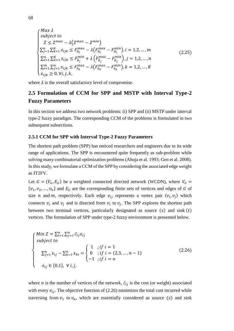
68

{


𝑍 ≤ 𝑍𝑚𝑎𝑥 − 𝜆(𝑍𝑚𝑎𝑥 − 𝑍𝑚𝑖𝑛)

∑ ∑ 𝑥𝑖𝑗𝑘𝐾𝑘=1

𝑛𝑗=1 ≤ 𝐹��𝑖

𝑚𝑎𝑥 − 𝜆(𝐹��𝑖𝑚𝑎𝑥 − 𝐹��𝑖

𝑚𝑖𝑛), 𝑖 = 1,2, … ,𝑚

∑ ∑ 𝑥𝑖𝑗𝑘𝐾𝑘=1

𝑛𝑖=1 ≤ 𝐹��𝑗

𝑚𝑖𝑛 + 𝜆 (𝐹��𝑗𝑚𝑎𝑥 − 𝐹��𝑗

𝑚𝑖𝑛) , 𝑗 = 1,2, … , 𝑛

∑ ∑ 𝑥𝑖𝑗𝑘𝑛𝑗=1

𝑚𝑖=1 ≤ 𝐹��𝑘

𝑚𝑎𝑥 − 𝜆(𝐹��𝑘𝑚𝑎𝑥 − 𝐹��𝑘

𝑚𝑖𝑛), 𝑘 = 1,2, … , 𝐾

𝑥𝑖𝑗𝑘 ≥ 0, ∀𝑖, 𝑗, 𝑘,

(2.25)

where 𝜆 is the overall satisfactory level of compromise.

2.5 Formulation of CCM for SPP and MSTP with Interval Type-2

Fuzzy Parameters

In this section we address two network problems: (i) SPP and (ii) MSTP under interval

type-2 fuzzy paradigm. The corresponding CCM of the problems is formulated in two

subsequent subsections.

2.5.1 CCM for SPP with Interval Type-2 Fuzzy Parameters

The shortest path problem (SPP) has enticed researchers and engineers due to its wide

range of applications. The SPP is encountered quite frequently as sub-problem while

solving many combinatorial optimization problems (Ahuja et al. 1993; Gen et al. 2008).

In this study, we formulate a CCM of the SPP by considering the associated edge weight

as IT2FV.

Let 𝐺 = (𝑉𝐺 , 𝐸𝐺) be a weighted connected directed network (WCDN), where 𝑉𝐺 =

{𝑣1, 𝑣2, … , 𝑣𝑛} and 𝐸𝐺 are the corresponding finite sets of vertices and edges of 𝐺 of

size 𝑛 and 𝑚, respectively. Each edge 𝑒𝑖𝑗 represents a vertex pair ⟨𝑣𝑖, 𝑣𝑗⟩ which

connects 𝑣𝑖 and 𝑣𝑗 and is directed from 𝑣𝑖 to 𝑣𝑗 . The SPP explores the shortest path

between two terminal vertices, particularly designated as source (𝑠) and sink (𝑡)

vertices. The formulation of SPP under type-2 fuzzy environment is presented below.

{

𝑀𝑖𝑛 𝑍 = ∑ ∑ ��𝑖𝑗𝑥𝑖𝑗

𝑛𝑗=1

𝑛𝑖=1


∑ 𝑥𝑖𝑗𝑛𝑗=1 − ∑ 𝑥𝑘𝑖

𝑛𝑘=1 = {

1 ; 𝑖𝑓 𝑖 = 1

0 ; 𝑖𝑓 𝑖 = (2,3, … , 𝑛 − 1)

−1 ; 𝑖𝑓 𝑖 = 𝑛

𝑥𝑖𝑗 ∈ {0,1}, ∀ 𝑖, 𝑗,

(2.26)

where 𝑛 is the number of vertices of the network, ��𝑖𝑗 is the cost (or weight) associated

with every 𝑒𝑖𝑗. The objective function of (2.26) minimizes the total cost incurred while

traversing from 𝑣1 to 𝑣𝑛, which are essentially considered as source (𝑠) and sink

69

(𝑡) vertices of 𝐺, respectively. The only constraint of (2.26) satisfies the flow

conservation law at all the vertices except 𝑠 and 𝑡. Every decision variable 𝑥𝑖𝑗 of (2.26)

accepts either 0 or 1. If 𝑥𝑖𝑗 = 1 then the corresponding edge 𝑒𝑖𝑗 is included in the

shortest path from 𝑠 to 𝑡, whereas if 𝑥𝑖𝑗 = 0, 𝑒𝑖𝑗 is excluded from the shortest path.

Here, each ��𝑖𝑗 associated with an edge 𝑒𝑖𝑗 is considered as an IT2FV and represented as

��𝑖𝑗 = (𝑐𝑖𝑗𝑈 , 𝑐𝑖𝑗

𝐿 ) = ((𝑐𝑖𝑗1𝑈 , 𝑐𝑖𝑗2

𝑈 , 𝑐𝑖𝑗3𝑈 , 𝑐𝑖𝑗4

𝑈 ; 𝑤𝑐𝑖𝑗𝑈 ) , (𝑐𝑖𝑗1

𝐿 , 𝑐𝑖𝑗2𝐿 , 𝑐𝑖𝑗3

𝐿 , 𝑐𝑖𝑗4𝐿 ; 𝑤𝑐𝑖𝑗

𝐿 )).

We formulate the chance-constrained model of the (2.26) following the steps as

mentioned in Section 2.3.2.

Step 1: Construct CCM for the model (2.26), considering the UMFs of the IT2FVs as

follows.

{


��𝑟{∑ ∑ ��𝑖𝑗𝑈𝑥𝑖𝑗

𝑛𝑗=1

𝑛𝑖=1 ≤ 𝑍 } ≥ 𝛿𝑈

𝑐𝑜𝑛𝑠𝑡𝑟𝑎𝑖𝑛𝑡𝑠 𝑜𝑓 (2.26),

(2.27)

where 𝛿𝑈 is the predetermined confidence level of the chance-constraint.

Step 2: Since ��𝑖𝑗𝑈 is a generalized trapezoidal fuzzy variable and 𝑥𝑖𝑗 is a binary variable,

so according to Theorem 2.2.1, the constraint ��𝑟{∑ ∑ ��𝑖𝑗𝑈𝑥𝑗

𝑛𝑗=1

𝑛𝑖=1 ≤ 𝑍 } ≥ 𝛿𝑈

equivalently becomes ∑ ∑ 𝐹𝑐��𝑗𝑈𝑥𝑖𝑗

𝑛𝑗=1

𝑛𝑖=1 ≤ 𝑍, where 𝐹𝑐��𝑗

𝑈 is given by

𝐹𝑐��𝑗𝑈 =

{

1

𝑤𝑐𝑖𝑗𝑈 ((𝑤𝑐𝑖𝑗

𝑈 − 2𝛿𝑈) 𝑐𝑖𝑗1𝑈 + 2𝛿𝑈𝑐𝑖𝑗2

𝑈 ) ; 𝑖𝑓 𝛿𝑈 ≤𝑤𝑐𝑖𝑗𝑈

2

1

𝑤𝑐𝑖𝑗𝑈 (2 (𝑤𝑐𝑖𝑗

𝑈 − 𝛿𝑈) 𝑐𝑖𝑗3𝑈 + (2𝛿𝑈 − 𝑤𝑐𝑖𝑗

𝑈 ) 𝑐𝑖𝑗4𝑈 ) ; 𝑖𝑓 𝛿𝑈 >

𝑤𝑐𝑖𝑗𝑈

2 .


{

𝑀𝑖𝑛 𝑍1 = ∑ ∑ 𝐹𝑐��𝑗𝑈𝑥𝑖𝑗

𝑛𝑗=1

𝑛𝑖=1


𝑐𝑜𝑛𝑠𝑡𝑟𝑎𝑖𝑛𝑡𝑠 𝑜𝑓 (2.26).

(2.28)

Step 3: Solve model (2.28) and suppose after solving we have 𝑀𝑖𝑛 𝑍1 = 𝑍′.

Step 4: Formulate CCM for the model (2.26), considering the LMFs of the IT2FVs as

follows.

{


��𝑟{∑ ∑ ��𝑖𝑗𝐿 𝑥𝑖𝑗

𝑛𝑗=1

𝑛𝑖=1 ≤ 𝑍 } ≥ 𝛿𝐿


(2.29)

where 𝛿𝐿 is the predetermined confidence level of the chance-constraint.

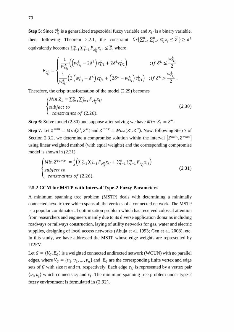
70

Step 5: Since ��𝑖𝑗𝐿 is a generalized trapezoidal fuzzy variable and 𝑥𝑖𝑗 is a binary variable,

then, following Theorem 2.2.1, the constraint ��𝑟{∑ ∑ ��𝑖𝑗𝐿 𝑥𝑗

𝑛𝑗=1

𝑛𝑖=1 ≤ 𝑍 } ≥ 𝛿𝐿

equivalently becomes ∑ ∑ 𝐹𝑐��𝑗𝐿 𝑥𝑖𝑗

𝑛𝑗=1

𝑛𝑖=1 ≤ 𝑍, where

𝐹𝑐��𝑗𝐿 =

{

1

𝑤𝑐𝑖𝑗𝐿((𝑤𝑐𝑖𝑗

𝐿 − 2𝛿𝐿) 𝑐𝑖𝑗1𝐿 + 2𝛿𝐿𝑐𝑖𝑗2

𝐿 ) ; 𝑖𝑓 𝛿𝐿 ≤𝑤𝑐𝑖𝑗𝐿

2

1

𝑤𝑐𝑖𝑗𝐿(2 (𝑤𝑐𝑖𝑗

𝐿 − 𝛿𝐿) 𝑐𝑖𝑗3𝐿 + (2𝛿𝐿 − 𝑤𝑐𝑖𝑗

𝐿 ) 𝑐𝑖𝑗4𝐿 ) ; 𝑖𝑓 𝛿𝐿 >

𝑤𝑐𝑖𝑗𝐿

2 .


{

𝑀𝑖𝑛 𝑍1 = ∑ ∑ 𝐹𝑐��𝑗𝐿 𝑥𝑖𝑗

𝑛𝑗=1

𝑛𝑖=1



(2.30)

Step 6: Solve model (2.30) and suppose after solving we have 𝑀𝑖𝑛 𝑍1 = 𝑍′′.

Step 7: Let 𝑍𝑚𝑖𝑛 = 𝑀𝑖𝑛(𝑍′, 𝑍′′) and 𝑍𝑚𝑎𝑥 = 𝑀𝑎𝑥(𝑍′, 𝑍′′). Now, following Step 7 of

Section 2.3.2, we determine a compromise solution within the interval [𝑍𝑚𝑖𝑛, 𝑍𝑚𝑎𝑥]

using linear weighted method (with equal weights) and the corresponding compromise

model is shown in (2.31).

{

𝑀𝑖𝑛 𝑍𝑐𝑜𝑚𝑝 =1

2(∑ ∑ 𝐹𝑐��𝑗

𝑈𝑥𝑖𝑗𝑛𝑗=1

𝑛𝑖=1 + ∑ ∑ 𝐹𝑐��𝑗

𝐿𝑥𝑖𝑗𝑛𝑗=1

𝑛𝑖=1 )



(2.31)

2.5.2 CCM for MSTP with Interval Type-2 Fuzzy Parameters

A minimum spanning tree problem (MSTP) deals with determining a minimally

connected acyclic tree which spans all the vertices of a connected network. The MSTP

is a popular combinatorial optimization problem which has received colossal attention

from researchers and engineers mainly due to its diverse application domains including

roadways or railways construction, laying of utility networks for gas, water and electric

supplies, designing of local access networks (Ahuja et al. 1993; Gen et al. 2008), etc.

In this study, we have addressed the MSTP whose edge weights are represented by

IT2FV.

Let 𝐺 = (𝑉𝐺 , 𝐸𝐺) is a weighted connected undirected network (WCUN) with no parallel

edges, where 𝑉𝐺 = {𝑣1, 𝑣2, … , 𝑣𝑛} and 𝐸𝐺 are the corresponding finite vertex and edge

sets of 𝐺 with size 𝑛 and 𝑚, respectively. Each edge 𝑒𝑖𝑗 is represented by a vertex pair

⟨𝑣𝑖 , 𝑣𝑗⟩ which connects 𝑣𝑖 and 𝑣𝑗 . The minimum spanning tree problem under type-2

fuzzy environment is formulated in (2.32).

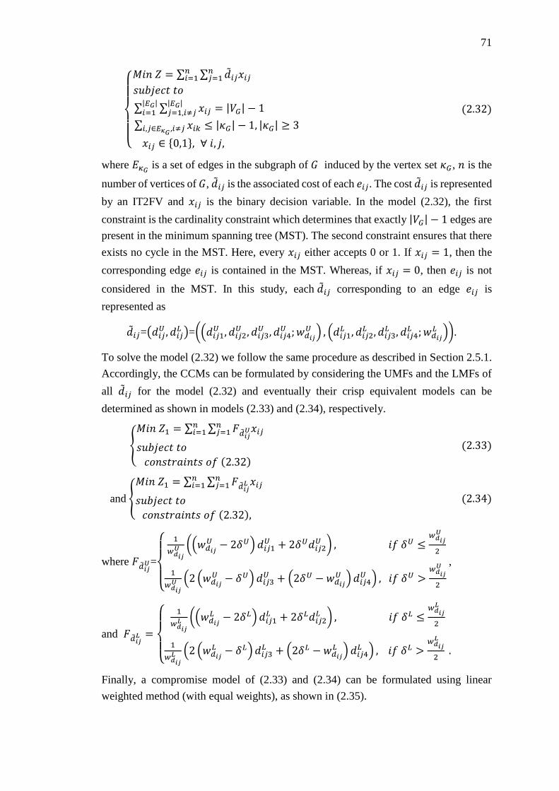
71

{

𝑀𝑖𝑛 𝑍 = ∑ ∑ ��𝑖𝑗𝑥𝑖𝑗

𝑛𝑗=1

𝑛𝑖=1


∑ ∑ 𝑥𝑖𝑗|𝐸𝐺|𝑗=1,𝑖≠𝑗

|𝐸𝐺|𝑖=1 = |𝑉𝐺| − 1

∑ 𝑥𝑖𝑘 ≤ |𝜅𝐺| − 1,𝑖,𝑗∈𝐸𝜅𝐺 ,𝑖≠𝑗|𝜅𝐺| ≥ 3

𝑥𝑖𝑗 ∈ {0,1}, ∀ 𝑖, 𝑗,

(2.32)

where 𝐸𝜅𝐺 is a set of edges in the subgraph of 𝐺 induced by the vertex set 𝜅𝐺 , 𝑛 is the

number of vertices of 𝐺, ��𝑖𝑗 is the associated cost of each 𝑒𝑖𝑗. The cost ��𝑖𝑗 is represented

by an IT2FV and 𝑥𝑖𝑗 is the binary decision variable. In the model (2.32), the first

constraint is the cardinality constraint which determines that exactly |𝑉𝐺| − 1 edges are

present in the minimum spanning tree (MST). The second constraint ensures that there

exists no cycle in the MST. Here, every 𝑥𝑖𝑗 either accepts 0 or 1. If 𝑥𝑖𝑗 = 1, then the

corresponding edge 𝑒𝑖𝑗 is contained in the MST. Whereas, if 𝑥𝑖𝑗 = 0, then 𝑒𝑖𝑗 is not

considered in the MST. In this study, each ��𝑖𝑗 corresponding to an edge 𝑒𝑖𝑗 is

represented as

��𝑖𝑗=(𝑑𝑖𝑗𝑈 , 𝑑𝑖𝑗

𝐿 )=((𝑑𝑖𝑗1𝑈 , 𝑑𝑖𝑗2

𝑈 , 𝑑𝑖𝑗3𝑈 , 𝑑𝑖𝑗4

𝑈 ; 𝑤𝑑𝑖𝑗𝑈 ) , (𝑑𝑖𝑗1

𝐿 , 𝑑𝑖𝑗2𝐿 , 𝑑𝑖𝑗3

𝐿 , 𝑑𝑖𝑗4𝐿 ; 𝑤𝑑𝑖𝑗

𝐿 )).

To solve the model (2.32) we follow the same procedure as described in Section 2.5.1.

Accordingly, the CCMs can be formulated by considering the UMFs and the LMFs of

all ��𝑖𝑗 for the model (2.32) and eventually their crisp equivalent models can be

determined as shown in models (2.33) and (2.34), respectively.

{

𝑀𝑖𝑛 𝑍1 = ∑ ∑ 𝐹��𝑖𝑗𝑈𝑥𝑖𝑗

𝑛𝑗=1

𝑛𝑖=1



(2.33)

and {

𝑀𝑖𝑛 𝑍1 = ∑ ∑ 𝐹��𝑖𝑗𝐿 𝑥𝑖𝑗

𝑛𝑗=1

𝑛𝑖=1



(2.34)

where 𝐹��𝑖𝑗𝑈=

{

1

𝑤𝑑𝑖𝑗𝑈 ((𝑤𝑑𝑖𝑗

𝑈 − 2𝛿𝑈) 𝑑𝑖𝑗1𝑈 + 2𝛿𝑈𝑑𝑖𝑗2

𝑈 ) , 𝑖𝑓 𝛿𝑈 ≤𝑤𝑑𝑖𝑗𝑈

2

1

𝑤𝑑𝑖𝑗𝑈 (2 (𝑤𝑑𝑖𝑗

𝑈 − 𝛿𝑈) 𝑑𝑖𝑗3𝑈 + (2𝛿𝑈 − 𝑤𝑑𝑖𝑗

𝑈 )𝑑𝑖𝑗4𝑈 ) , 𝑖𝑓 𝛿𝑈 >

𝑤𝑑𝑖𝑗𝑈

2

,

and 𝐹��𝑖𝑗𝐿 =

{

1

𝑤𝑑𝑖𝑗𝐿 ((𝑤𝑑𝑖𝑗

𝐿 − 2𝛿𝐿)𝑑𝑖𝑗1𝐿 + 2𝛿𝐿𝑑𝑖𝑗2

𝐿 ) , 𝑖𝑓 𝛿𝐿 ≤𝑤𝑑𝑖𝑗𝐿

2

1

𝑤𝑑𝑖𝑗𝐿 (2 (𝑤𝑑𝑖𝑗

𝐿 − 𝛿𝐿)𝑑𝑖𝑗3𝐿 + (2𝛿𝐿 − 𝑤𝑑𝑖𝑗

𝐿 ) 𝑑𝑖𝑗4𝐿 ) , 𝑖𝑓 𝛿𝐿 >

𝑤𝑑𝑖𝑗𝐿

2 .

Finally, a compromise model of (2.33) and (2.34) can be formulated using linear

weighted method (with equal weights), as shown in (2.35).

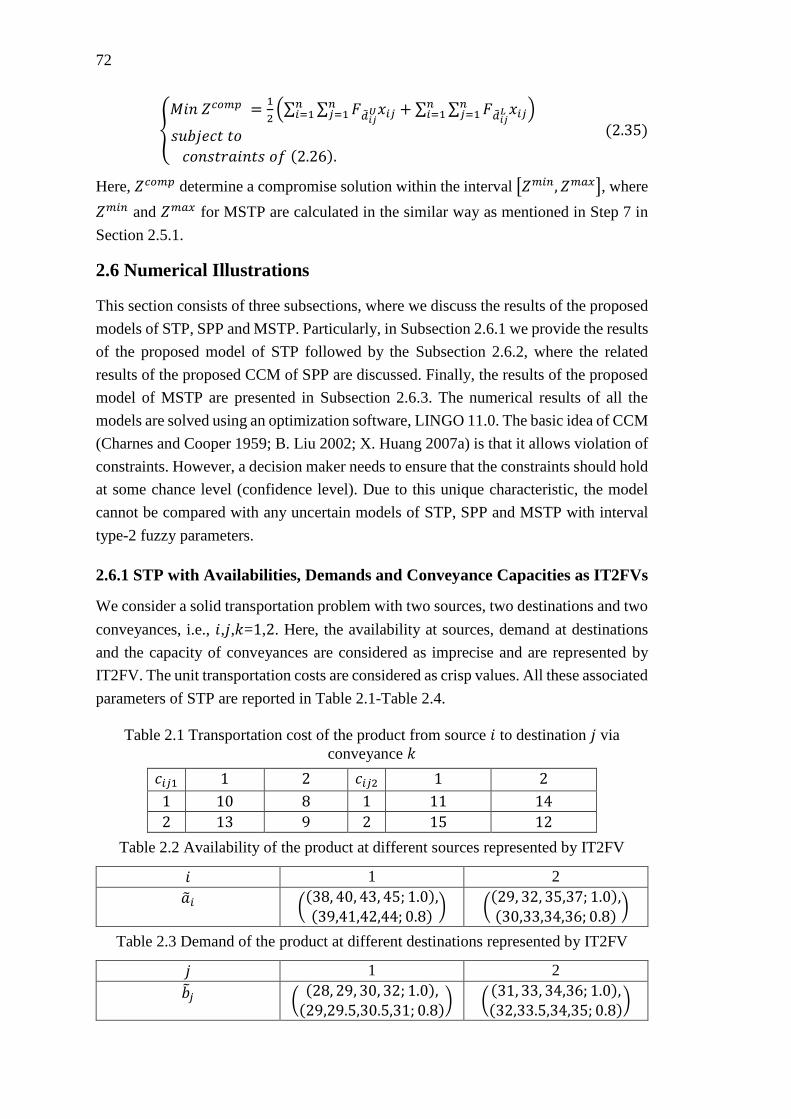
72

{

𝑀𝑖𝑛 𝑍𝑐𝑜𝑚𝑝 =1

2(∑ ∑ 𝐹��𝑖𝑗

𝑈𝑥𝑖𝑗𝑛𝑗=1

𝑛𝑖=1 + ∑ ∑ 𝐹��𝑖𝑗

𝐿 𝑥𝑖𝑗𝑛𝑗=1

𝑛𝑖=1 )



(2.35)

Here, 𝑍𝑐𝑜𝑚𝑝 determine a compromise solution within the interval [𝑍𝑚𝑖𝑛, 𝑍𝑚𝑎𝑥], where

𝑍𝑚𝑖𝑛 and 𝑍𝑚𝑎𝑥 for MSTP are calculated in the similar way as mentioned in Step 7 in

Section 2.5.1.

2.6 Numerical Illustrations

This section consists of three subsections, where we discuss the results of the proposed

models of STP, SPP and MSTP. Particularly, in Subsection 2.6.1 we provide the results

of the proposed model of STP followed by the Subsection 2.6.2, where the related

results of the proposed CCM of SPP are discussed. Finally, the results of the proposed

model of MSTP are presented in Subsection 2.6.3. The numerical results of all the

models are solved using an optimization software, LINGO 11.0. The basic idea of CCM

(Charnes and Cooper 1959; B. Liu 2002; X. Huang 2007a) is that it allows violation of

constraints. However, a decision maker needs to ensure that the constraints should hold

at some chance level (confidence level). Due to this unique characteristic, the model

cannot be compared with any uncertain models of STP, SPP and MSTP with interval

type-2 fuzzy parameters.

2.6.1 STP with Availabilities, Demands and Conveyance Capacities as IT2FVs

We consider a solid transportation problem with two sources, two destinations and two

conveyances, i.e., 𝑖,𝑗,𝑘=1,2. Here, the availability at sources, demand at destinations

and the capacity of conveyances are considered as imprecise and are represented by

IT2FV. The unit transportation costs are considered as crisp values. All these associated

parameters of STP are reported in Table 2.1-Table 2.4.

Table 2.1 Transportation cost of the product from source 𝑖 to destination 𝑗 via

conveyance 𝑘

𝑐𝑖𝑗1 1 2 𝑐𝑖𝑗2 1 2

1 10 8 1 11 14

2 13 9 2 15 12

Table 2.2 Availability of the product at different sources represented by IT2FV

𝑖 1 2

��𝑖 ((38, 40, 43, 45; 1.0),(39,41,42,44; 0.8)

) ((29, 32, 35,37; 1.0),(30,33,34,36; 0.8)

)

Table 2.3 Demand of the product at different destinations represented by IT2FV

𝑗 1 2

��𝑗 ((28, 29, 30, 32; 1.0),(29,29.5,30.5,31; 0.8)

) ((31, 33, 34,36; 1.0),(32,33.5,34,35; 0.8)

)

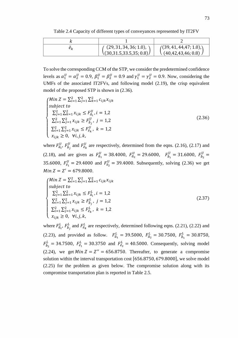
73

Table 2.4 Capacity of different types of conveyances represented by IT2FV

𝑘 1 2

��𝑘 ((29, 31, 34, 36; 1.0),(30,31.5,33.5,35; 0.8)

) ((39, 41, 44,47; 1.0),(40,42,43,46; 0.8)

)

To solve the corresponding CCM of the STP, we consider the predetermined confidence

levels as 𝛼1𝑈 = 𝛼2

𝑈 = 0.9, 𝛽1𝑈 = 𝛽2

𝑈 = 0.9 and 𝛾1𝑈 = 𝛾2

𝑈 = 0.9. Now, considering the

UMFs of the associated IT2FVs, and following model (2.19), the crisp equivalent

model of the proposed STP is shown in (2.36).

{


2𝑘=1

2𝑗=1

2𝑖=1


∑ ∑ 𝑥𝑖𝑗𝑘 ≤ 𝐹��𝑖𝑈2

𝑘=12𝑗=1 , 𝑖 = 1,2

∑ ∑ 𝑥𝑖𝑗𝑘 ≥ 𝐹��𝑗𝑈2

𝑗=1 , 𝑗 = 1,22𝑖=1

∑ ∑ 𝑥𝑖𝑗𝑘 ≤ 𝐹��𝑘𝑈2

𝑗=1 , 𝑘 = 1,22𝑖=1

𝑥𝑖𝑗𝑘 ≥ 0, ∀𝑖, 𝑗, 𝑘,

(2.36)

where 𝐹��𝑖𝑈, 𝐹��𝑗

𝑈 and 𝐹��𝑘𝑈 are respectively, determined from the eqns. (2.16), (2.17) and

(2.18), and are given as 𝐹��1𝑈 = 38.4000, 𝐹��2

𝑈 = 29.6000, 𝐹��1𝑈 = 31.6000, 𝐹��2

𝑈 =

35.6000, 𝐹��1𝑈 = 29.4000 and 𝐹��2

𝑈 = 39.4000. Subsequently, solving (2.36) we get

𝑀𝑖𝑛 𝑍 = 𝑍′ = 679.8000.

{


2𝑘=1

2𝑗=1

2𝑖=1


∑ ∑ 𝑥𝑖𝑗𝑘 ≤ 𝐹��𝑖𝐿2

𝑘=12𝑗=1 , 𝑖 = 1,2

∑ ∑ 𝑥𝑖𝑗𝑘 ≥ 𝐹��𝑗𝐿2

𝑗=1 , 𝑗 = 1,22𝑖=1

∑ ∑ 𝑥𝑖𝑗𝑘 ≤ 𝐹��𝑘𝐿2

𝑗=1 , 𝑘 = 1,22𝑖=1

𝑥𝑖𝑗𝑘 ≥ 0, ∀𝑖, 𝑗, 𝑘,

(2.37)

where 𝐹��𝑖𝐿 , 𝐹��𝑗

𝐿 and 𝐹��𝑘𝐿 are respectively, determined following eqns. (2.21), (2.22) and

(2.23), and provided as follow. 𝐹��1𝐿 = 39.5000, 𝐹��2

𝐿 = 30.7500, 𝐹��1𝐿 = 30.8750,

𝐹��2𝐿 = 34.7500, 𝐹��1

𝐿 = 30.3750 and 𝐹��2𝐿 = 40.5000. Consequently, solving model

(2.24), we get 𝑀𝑖𝑛 𝑍 = 𝑍′′ = 656.8750. Thereafter, to generate a compromise

solution within the interval transportation cost [656.8750, 679.8000], we solve model

(2.25) for the problem as given below. The compromise solution along with its

compromise transportation plan is reported in Table 2.5.

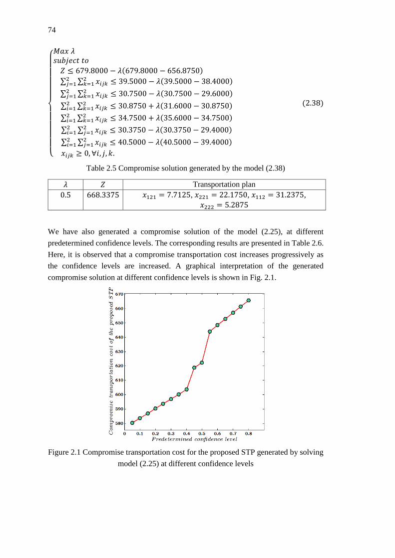
74

{


𝑍 ≤ 679.8000 − 𝜆(679.8000 − 656.8750)

∑ ∑ 𝑥𝑖𝑗𝑘2𝑘=1

2𝑗=1 ≤ 39.5000 − 𝜆(39.5000 − 38.4000)


2𝑗=1 ≤ 30.7500 − 𝜆(30.7500 − 29.6000)


2𝑖=1 ≤ 30.8750 + 𝜆(31.6000 − 30.8750)


2𝑖=1 ≤ 34.7500 + 𝜆(35.6000 − 34.7500)

∑ ∑ 𝑥𝑖𝑗𝑘2𝑗=1

2𝑖=1 ≤ 30.3750 − 𝜆(30.3750 − 29.4000)

∑ ∑ 𝑥𝑖𝑗𝑘2𝑗=1

2𝑖=1 ≤ 40.5000 − 𝜆(40.5000 − 39.4000)

𝑥𝑖𝑗𝑘 ≥ 0, ∀𝑖, 𝑗, 𝑘.

(2.38)

Table 2.5 Compromise solution generated by the model (2.38)

𝜆 𝑍 Transportation plan

0.5 668.3375 𝑥121 = 7.7125, 𝑥221 = 22.1750, 𝑥112 = 31.2375,

𝑥222 = 5.2875

We have also generated a compromise solution of the model (2.25), at different

predetermined confidence levels. The corresponding results are presented in Table 2.6.

Here, it is observed that a compromise transportation cost increases progressively as

the confidence levels are increased. A graphical interpretation of the generated

compromise solution at different confidence levels is shown in Fig. 2.1.

Figure 2.1 Compromise transportation cost for the proposed STP generated by solving

model (2.25) at different confidence levels

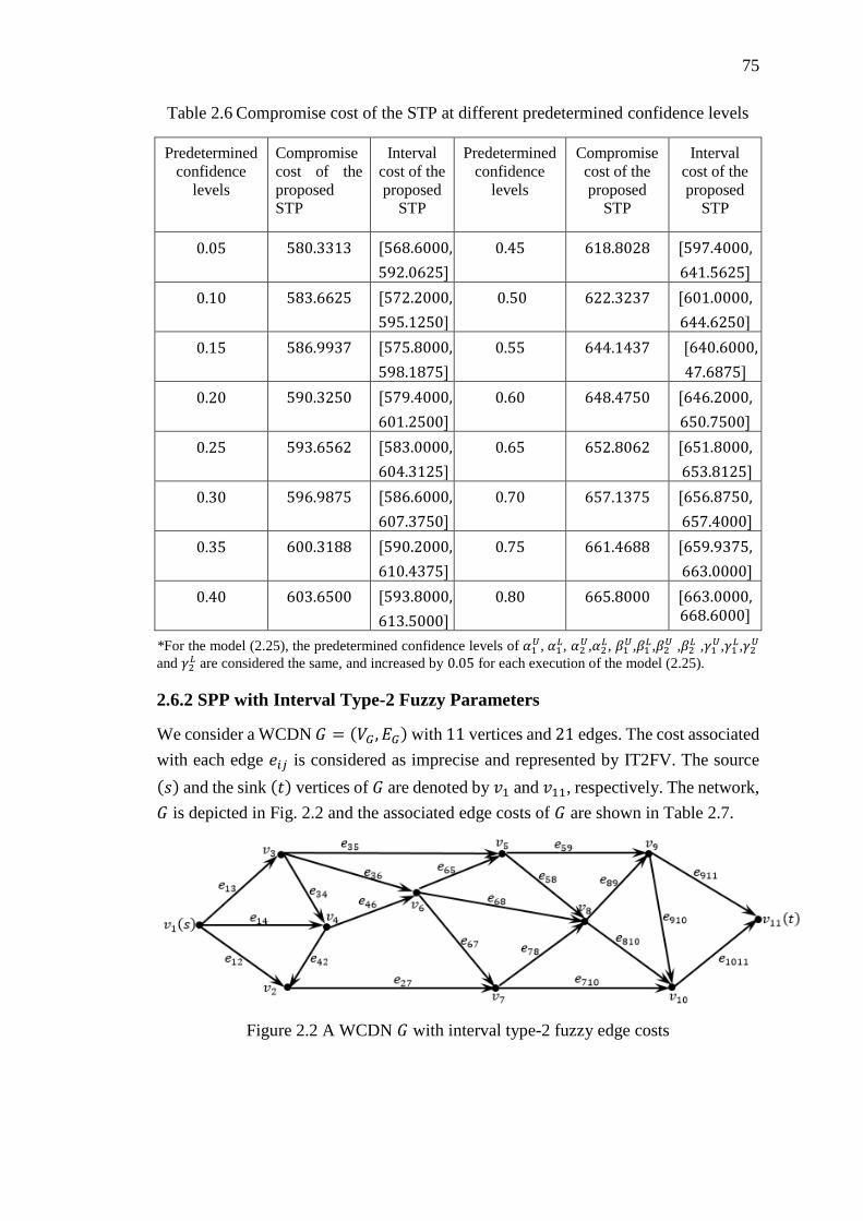
75

Table 2.6 Compromise cost of the STP at different predetermined confidence levels

Predetermined

confidence

levels

Compromise

cost of the

proposed

STP

Interval

cost of the

proposed

STP

Predetermined

confidence

levels

Compromise

cost of the

proposed

STP

Interval

cost of the

proposed

STP

0.05 580.3313 [568.6000,

592.0625]

0.45 618.8028 [597.4000,

641.5625]

0.10 583.6625 [572.2000,

595.1250]

0.50 622.3237 [601.0000,

644.6250]

0.15 586.9937 [575.8000,

598.1875]

0.55 644.1437 [640.6000,

47.6875]

0.20 590.3250 [579.4000,

601.2500]

0.60 648.4750 [646.2000,

650.7500]

0.25 593.6562 [583.0000,

604.3125]

0.65 652.8062 [651.8000,

653.8125]

0.30 596.9875 [586.6000,

607.3750]

0.70 657.1375 [656.8750,

657.4000]

0.35 600.3188 [590.2000,

610.4375]

0.75 661.4688 [659.9375,

663.0000]

0.40 603.6500 [593.8000,

613.5000]

0.80 665.8000 [663.0000, 668.6000]

*For the model (2.25), the predetermined confidence levels of 𝛼1𝑈, 𝛼1

𝐿, 𝛼2𝑈,𝛼2

𝐿, 𝛽1𝑈,𝛽1

𝐿,𝛽2𝑈 ,𝛽2

𝐿 ,𝛾1𝑈,𝛾1

𝐿,𝛾2𝑈

and 𝛾2𝐿 are considered the same, and increased by 0.05 for each execution of the model (2.25).

2.6.2 SPP with Interval Type-2 Fuzzy Parameters

We consider a WCDN 𝐺 = (𝑉𝐺 , 𝐸𝐺) with 11 vertices and 21 edges. The cost associated

with each edge 𝑒𝑖𝑗 is considered as imprecise and represented by IT2FV. The source

(𝑠) and the sink (𝑡) vertices of 𝐺 are denoted by 𝑣1 and 𝑣11, respectively. The network,

𝐺 is depicted in Fig. 2.2 and the associated edge costs of 𝐺 are shown in Table 2.7.

Figure 2.2 A WCDN 𝐺 with interval type-2 fuzzy edge costs

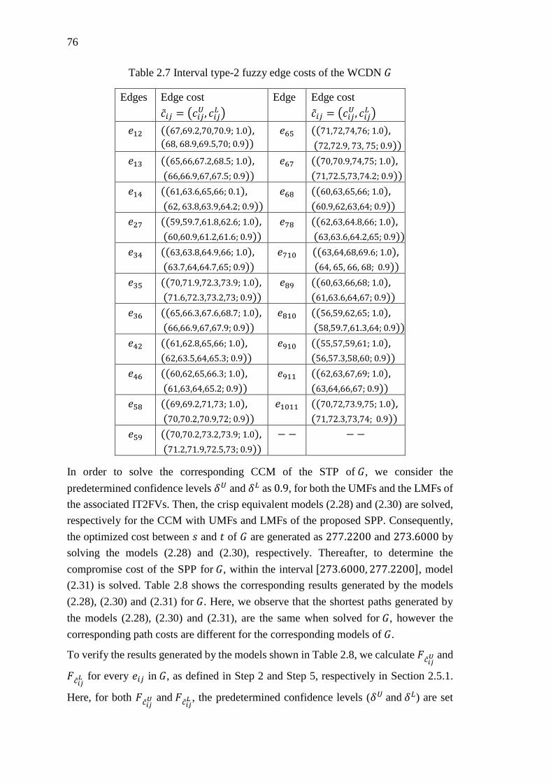
76

Table 2.7 Interval type-2 fuzzy edge costs of the WCDN 𝐺

Edges Edge cost


𝐿 )

Edge Edge cost


𝐿 )

𝑒12 ((67,69.2,70,70.9; 1.0), (68, 68.9,69.5,70; 0.9))

𝑒65 ((71,72,74,76; 1.0),

(72,72.9, 73, 75; 0.9))

𝑒13 ((65,66,67.2,68.5; 1.0),

(66,66.9,67,67.5; 0.9))

𝑒67 ((70,70.9,74,75; 1.0),

(71,72.5,73,74.2; 0.9))

𝑒14 ((61,63.6,65,66; 0.1),

(62, 63.8,63.9,64.2; 0.9))

𝑒68 ((60,63,65,66; 1.0),

(60.9,62,63,64; 0.9))

𝑒27 ((59,59.7,61.8,62.6; 1.0),

(60,60.9,61.2,61.6; 0.9))

𝑒78 ((62,63,64.8,66; 1.0),

(63,63.6,64.2,65; 0.9))

𝑒34 ((63,63.8,64.9,66; 1.0),

(63.7,64,64.7,65; 0.9))

𝑒710 ((63,64,68,69.6; 1.0),

(64, 65, 66, 68; 0.9))

𝑒35 ((70,71.9,72.3,73.9; 1.0),

(71.6,72.3,73.2,73; 0.9))

𝑒89 ((60,63,66,68; 1.0),

(61,63.6,64,67; 0.9))

𝑒36 ((65,66.3,67.6,68.7; 1.0),

(66,66.9,67,67.9; 0.9))

𝑒810 ((56,59,62,65; 1.0),

(58,59.7,61.3,64; 0.9))

𝑒42 ((61,62.8,65,66; 1.0),

(62,63.5,64,65.3; 0.9))

𝑒910 ((55,57,59,61; 1.0),

(56,57.3,58,60; 0.9))

𝑒46 ((60,62,65,66.3; 1.0),

(61,63,64,65.2; 0.9))

𝑒911 ((62,63,67,69; 1.0),

(63,64,66,67; 0.9))

𝑒58 ((69,69.2,71,73; 1.0),

(70,70.2,70.9,72; 0.9))

𝑒1011 ((70,72,73.9,75; 1.0),

(71,72.3,73,74; 0.9))

𝑒59 ((70,70.2,73.2,73.9; 1.0),

(71.2,71.9,72.5,73; 0.9))

−− −−

In order to solve the corresponding CCM of the STP of 𝐺, we consider the

predetermined confidence levels 𝛿𝑈 and 𝛿𝐿 as 0.9, for both the UMFs and the LMFs of

the associated IT2FVs. Then, the crisp equivalent models (2.28) and (2.30) are solved,

respectively for the CCM with UMFs and LMFs of the proposed SPP. Consequently,

the optimized cost between 𝑠 and 𝑡 of 𝐺 are generated as 277.2200 and 273.6000 by

solving the models (2.28) and (2.30), respectively. Thereafter, to determine the

compromise cost of the SPP for 𝐺, within the interval [273.6000, 277.2200], model

(2.31) is solved. Table 2.8 shows the corresponding results generated by the models

(2.28), (2.30) and (2.31) for 𝐺. Here, we observe that the shortest paths generated by

the models (2.28), (2.30) and (2.31), are the same when solved for 𝐺, however the

corresponding path costs are different for the corresponding models of 𝐺.

To verify the results generated by the models shown in Table 2.8, we calculate 𝐹𝑐��𝑗𝑈 and

𝐹𝑐��𝑗𝐿 for every 𝑒𝑖𝑗 in 𝐺, as defined in Step 2 and Step 5, respectively in Section 2.5.1.

Here, for both 𝐹𝑐��𝑗𝑈 and 𝐹𝑐��𝑗

𝐿 , the predetermined confidence levels (𝛿𝑈 and 𝛿𝐿) are set

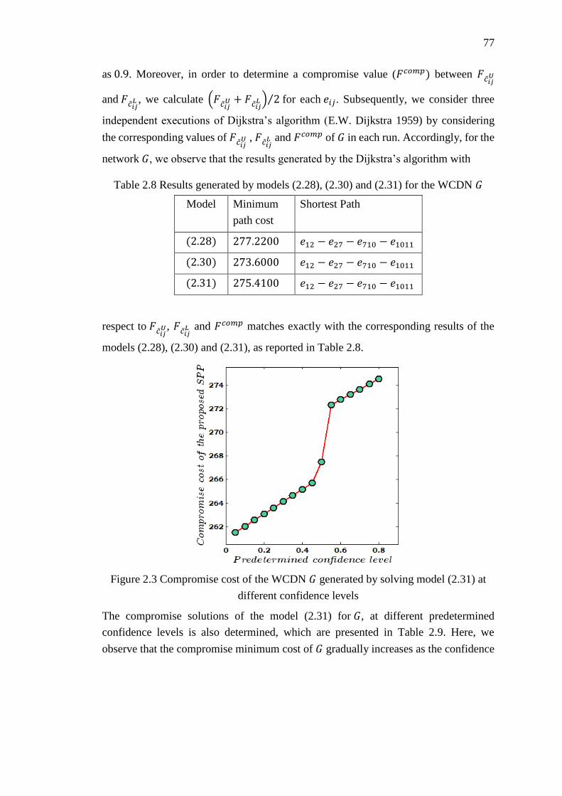
77

as 0.9. Moreover, in order to determine a compromise value (𝐹𝑐𝑜𝑚𝑝) between 𝐹𝑐��𝑗𝑈

and 𝐹𝑐��𝑗𝐿 , we calculate (𝐹𝑐��𝑗

𝑈 + 𝐹𝑐��𝑗𝐿 ) 2⁄ for each 𝑒𝑖𝑗. Subsequently, we consider three

independent executions of Dijkstra’s algorithm (E.W. Dijkstra 1959) by considering

the corresponding values of 𝐹𝑐��𝑗𝑈 , 𝐹𝑐��𝑗

𝐿 and 𝐹𝑐𝑜𝑚𝑝 of 𝐺 in each run. Accordingly, for the

network 𝐺, we observe that the results generated by the Dijkstra’s algorithm with

Table 2.8 Results generated by models (2.28), (2.30) and (2.31) for the WCDN 𝐺

Model Minimum

path cost

Shortest Path

(2.28) 277.2200 𝑒12 − 𝑒27 − 𝑒710 − 𝑒1011

(2.30) 273.6000 𝑒12 − 𝑒27 − 𝑒710 − 𝑒1011

(2.31) 275.4100 𝑒12 − 𝑒27 − 𝑒710 − 𝑒1011

respect to 𝐹𝑐��𝑗𝑈, 𝐹𝑐��𝑗

𝐿 and 𝐹𝑐𝑜𝑚𝑝 matches exactly with the corresponding results of the

models (2.28), (2.30) and (2.31), as reported in Table 2.8.

Figure 2.3 Compromise cost of the WCDN 𝐺 generated by solving model (2.31) at

different confidence levels

The compromise solutions of the model (2.31) for 𝐺, at different predetermined

confidence levels is also determined, which are presented in Table 2.9. Here, we

observe that the compromise minimum cost of 𝐺 gradually increases as the confidence

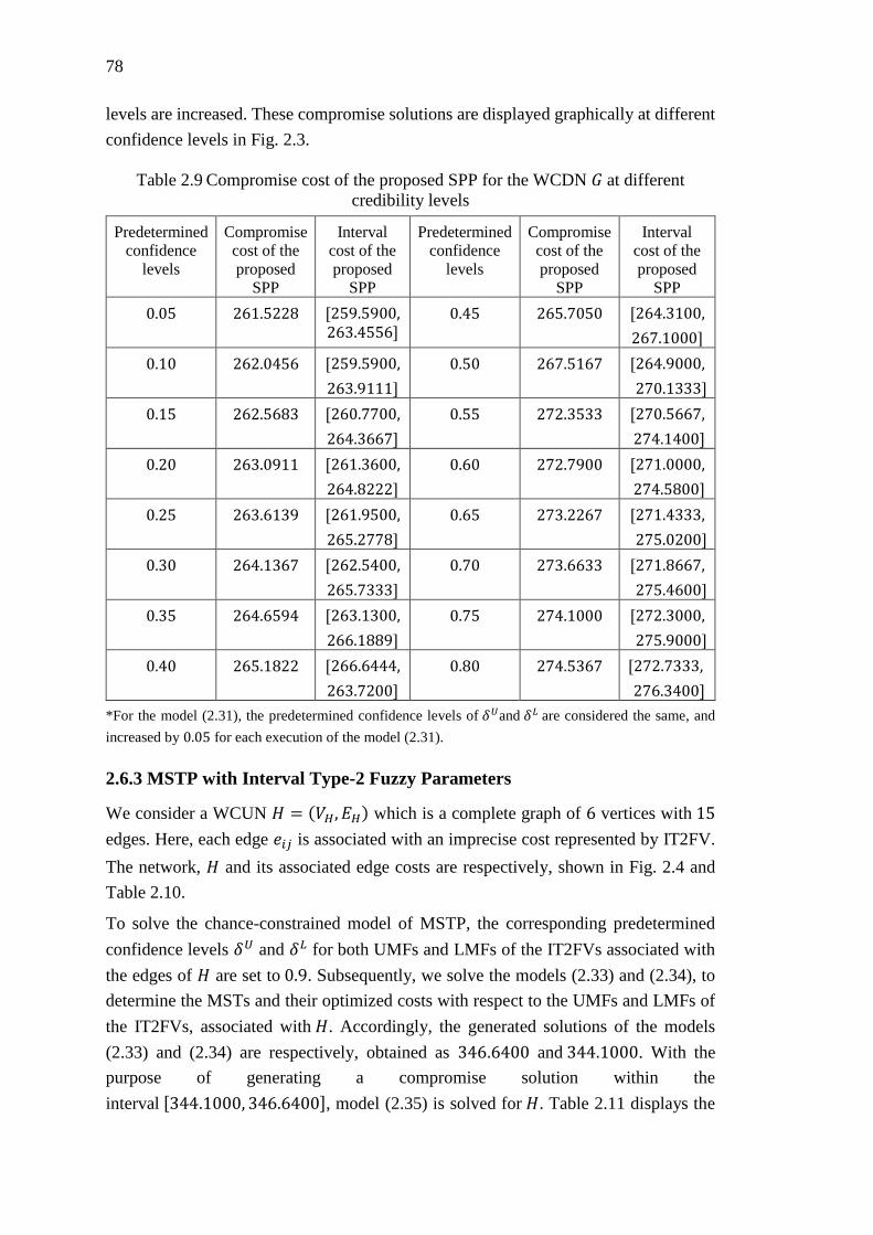
78

levels are increased. These compromise solutions are displayed graphically at different

confidence levels in Fig. 2.3.

Table 2.9 Compromise cost of the proposed SPP for the WCDN 𝐺 at different

credibility levels

Predetermined

confidence

levels

Compromise

cost of the

proposed

SPP

Interval

cost of the

proposed

SPP

Predetermined

confidence

levels

Compromise

cost of the

proposed

SPP

Interval

cost of the

proposed

SPP

0.05 261.5228 [259.5900, 263.4556]

0.45 265.7050 [264.3100,

267.1000]

0.10 262.0456 [259.5900,

263.9111]

0.50 267.5167 [264.9000,

270.1333]

0.15 262.5683 [260.7700,

264.3667]

0.55 272.3533 [270.5667,

274.1400]

0.20 263.0911 [261.3600,

264.8222]

0.60 272.7900 [271.0000,

274.5800]

0.25 263.6139 [261.9500,

265.2778]

0.65 273.2267 [271.4333,

275.0200]

0.30 264.1367 [262.5400,

265.7333]

0.70 273.6633 [271.8667,

275.4600]

0.35 264.6594 [263.1300,

266.1889]

0.75 274.1000 [272.3000,

275.9000]

0.40 265.1822 [266.6444,

263.7200]

0.80 274.5367 [272.7333,

276.3400]

*For the model (2.31), the predetermined confidence levels of 𝛿𝑈and 𝛿𝐿 are considered the same, and

increased by 0.05 for each execution of the model (2.31).

2.6.3 MSTP with Interval Type-2 Fuzzy Parameters

We consider a WCUN 𝐻 = (𝑉𝐻, 𝐸𝐻) which is a complete graph of 6 vertices with 15

edges. Here, each edge 𝑒𝑖𝑗 is associated with an imprecise cost represented by IT2FV.

The network, 𝐻 and its associated edge costs are respectively, shown in Fig. 2.4 and

Table 2.10.

To solve the chance-constrained model of MSTP, the corresponding predetermined

confidence levels 𝛿𝑈 and 𝛿𝐿 for both UMFs and LMFs of the IT2FVs associated with

the edges of 𝐻 are set to 0.9. Subsequently, we solve the models (2.33) and (2.34), to

determine the MSTs and their optimized costs with respect to the UMFs and LMFs of

the IT2FVs, associated with 𝐻. Accordingly, the generated solutions of the models

(2.33) and (2.34) are respectively, obtained as 346.6400 and 344.1000. With the

purpose of generating a compromise solution within the

interval [344.1000, 346.6400], model (2.35) is solved for 𝐻. Table 2.11 displays the

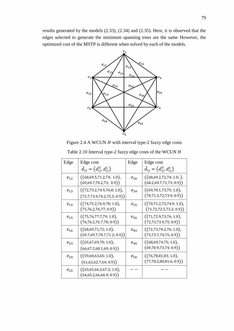
79

results generated by the models (2.33), (2.34) and (2.35). Here, it is observed that the

edges selected to generate the minimum spanning trees are the same However, the

optimized cost of the MSTP is different when solved by each of the models.

Figure 2.4 A WCUN 𝐻 with interval type-2 fuzzy edge costs

Table 2.10 Interval type-2 fuzzy edge costs of the WCUN 𝐻

Edge Edge cost

��𝑖𝑗 = (𝑑𝑖𝑗𝑈 , 𝑑𝑖𝑗

𝐿 )

Edge Edge cost

��𝑖𝑗 = (𝑑𝑖𝑗𝑈 , 𝑑𝑖𝑗

𝐿 )

𝑒12 ((68,69.5,71.2,74; 1.0), (69,69.7,70.2,73; 0.9))

𝑒26 ((68,69.2,72,74; 1.0; ), (68.2,69.7,71,73; 0.9))

𝑒13 ((72,73.2,74.9,76.8; 1.0),

(72.7,73.9,74.2,75.5; 0.9))

𝑒34 ((69,70.1,73,75; 1.0), (70,71.3,72,73.9; 0.9))

𝑒14 ((74,75.2,76.9,78; 1.0), (75,76.2,76,77; 0.9))

𝑒35 ((70,71.2,73,74.9; 1.0), (71,72,72.5,73.2; 0.9))

𝑒15 ((75,76,77.7,79; 1.0), (76,76.2,76.7,78; 0.9))

𝑒36 ((71,72.9,73,76; 1.0), (72,73,73.9,75; 0.9))

𝑒16 ((68,69,71,72; 1.0), (69.7,69.7,70.7,71.2; 0.9))

𝑒45 ((72,73,74.2,76; 1.0), (73,73.7,74,75; 0.9))

𝑒23 ((65,67,69,70; 1.0),

(66,67.2,68.1,69; 0.9))

𝑒46 ((68,69,74,75; 1.0), (69,70.9,73,74; 0.9))

𝑒24 ((59,60,63,65; 1.0),

(61,62,62.7,64; 0.9))

𝑒56 ((76,78,81,83; 1.0), (77,78.2,80,81.6; 0.9))

𝑒25 ((63,65,66.2,67.2; 1.0), (64,65.2,66,66.9; 0.9))

−− −−

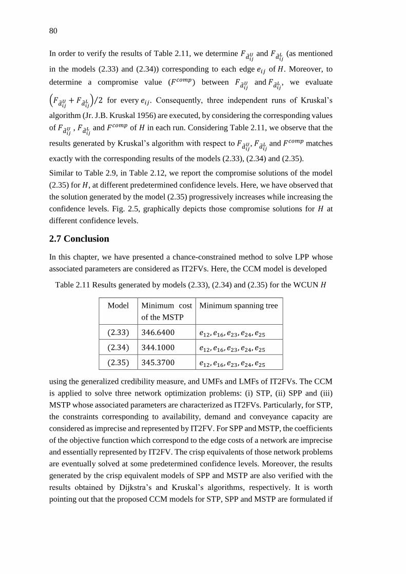
80

In order to verify the results of Table 2.11, we determine 𝐹��𝑖𝑗𝑈 and 𝐹��𝑖𝑗

𝐿 (as mentioned

in the models (2.33) and (2.34)) corresponding to each edge 𝑒𝑖𝑗 of 𝐻. Moreover, to

determine a compromise value (𝐹𝑐𝑜𝑚𝑝) between 𝐹��𝑖𝑗𝑈 and 𝐹��𝑖𝑗

𝐿 , we evaluate

(𝐹��𝑖𝑗𝑈 + 𝐹��𝑖𝑗

𝐿 ) 2⁄ for every 𝑒𝑖𝑗. Consequently, three independent runs of Kruskal’s

algorithm (Jr. J.B. Kruskal 1956) are executed, by considering the corresponding values

of 𝐹��𝑖𝑗𝑈 , 𝐹��𝑖𝑗

𝐿 and 𝐹𝑐𝑜𝑚𝑝 of 𝐻 in each run. Considering Table 2.11, we observe that the

results generated by Kruskal’s algorithm with respect to 𝐹��𝑖𝑗𝑈 , 𝐹��𝑖𝑗

𝐿 and 𝐹𝑐𝑜𝑚𝑝 matches

exactly with the corresponding results of the models (2.33), (2.34) and (2.35).

Similar to Table 2.9, in Table 2.12, we report the compromise solutions of the model

(2.35) for 𝐻, at different predetermined confidence levels. Here, we have observed that

the solution generated by the model (2.35) progressively increases while increasing the

confidence levels. Fig. 2.5, graphically depicts those compromise solutions for 𝐻 at

different confidence levels.

2.7 Conclusion

In this chapter, we have presented a chance-constrained method to solve LPP whose

associated parameters are considered as IT2FVs. Here, the CCM model is developed

Table 2.11 Results generated by models (2.33), (2.34) and (2.35) for the WCUN 𝐻

Model Minimum cost

of the MSTP

Minimum spanning tree

(2.33) 346.6400 𝑒12, 𝑒16, 𝑒23, 𝑒24, 𝑒25

(2.34) 344.1000 𝑒12, 𝑒16, 𝑒23, 𝑒24, 𝑒25

(2.35) 345.3700 𝑒12, 𝑒16, 𝑒23, 𝑒24, 𝑒25

using the generalized credibility measure, and UMFs and LMFs of IT2FVs. The CCM

is applied to solve three network optimization problems: (i) STP, (ii) SPP and (iii)

MSTP whose associated parameters are characterized as IT2FVs. Particularly, for STP,

the constraints corresponding to availability, demand and conveyance capacity are

considered as imprecise and represented by IT2FV. For SPP and MSTP, the coefficients

of the objective function which correspond to the edge costs of a network are imprecise

and essentially represented by IT2FV. The crisp equivalents of those network problems

are eventually solved at some predetermined confidence levels. Moreover, the results

generated by the crisp equivalent models of SPP and MSTP are also verified with the

results obtained by Dijkstra’s and Kruskal’s algorithms, respectively. It is worth

pointing out that the proposed CCM models for STP, SPP and MSTP are formulated if

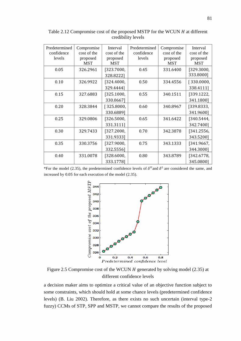
81

Table 2.12 Compromise cost of the proposed MSTP for the WCUN 𝐻 at different

credibility levels

*For the model (2.35), the predetermined confidence levels of 𝛿𝑈and 𝛿𝐿 are considered the same, and

increased by 0.05 for each execution of the model (2.35).

Figure 2.5 Compromise cost of the WCUN 𝐻 generated by solving model (2.35) at

different confidence levels

a decision maker aims to optimize a critical value of an objective function subject to

some constraints, which should hold at some chance levels (predetermined confidence

levels) (B. Liu 2002). Therefore, as there exists no such uncertain (interval type-2

fuzzy) CCMs of STP, SPP and MSTP, we cannot compare the results of the proposed

Predetermined

confidence

levels

Compromise

cost of the

proposed

MST

Interval

cost of the

proposed

MST

Predetermined

confidence

levels

Compromise

cost of the

proposed

MST

Interval

cost of the

proposed

MST

0.05 326.2961 [323.7000,

328.8222]

0.45 331.6400 [329.3000,333.8000]

0.10 326.9922 [324.4000,

329.4444]

0.50 334.4556 [ 330.0000,

338.4111]

0.15 327.6883 [325.1000,

330.0667]

0.55 340.1511 [339.1222,

341.1800]

0.20 328.3844 [ 325.8000,

330.6889]

0.60 340.8967 [339.8333,

341.9600]

0.25 329.0806 [326.5000,

331.3111]

0.65 341.6422 [340.5444,

342.7400]

0.30 329.7433 [327.2000,

331.9333]

0.70 342.3878 [341.2556,

343.5200]

0.35 330.3756 [327.9000,

332.5556]

0.75 343.1333 [341.9667,

344.3000]

0.40 331.0078 [328.6000,

333.1778]

0.80 343.8789 [342.6778,

345.0800]

82

models in the process of decision making. The usage of the model is solely dependent

on the decision maker’s preference.

In future, we would like to apply the proposed CCM to different optimization problems

including portfolio selection, inventory management and supply chain management. In

addition, the proposed CCM model can be modified for the generalized T2FVs to solve

the different single and multi-objective optimization problems.

83

Chapter 3

Genetic Algorithm with Varying

Population for Random Fuzzy

Maximum Flow Problem

User

Text Box

84

User

Text Box

85

Chapter 3

Genetic Algorithm with Varying Population

for Random Fuzzy Maximum Flow Problem

3.1 Introduction

Maximum flow problem (MFP) is one of the popular network optimization problems

which has captivated many researchers due to its wide application domains including

VLSI design, electrical power distribution system, logistic network, transportation

network, computer network, etc. The genesis of MFP has its connection with the Soviet

railway project which was underway in Eastern Europe (Harris and Ross 1955). The

first algorithm to solve the maximum flow problem is presented by Ford and Fulkerson

(1956). Subsequently, the MFP is further investigated by Ford and Fulkerson (1962).

Thereafter, various researchers (E.A. Dinic 1970; Edmonds and Karp 1972; A.V.

Karzanov 1974; R.E. Tarjan 1984; Goldberg and Tarjan 1986; Ahuja and Orlin 1989;

Hachtel and Somenzi 1997) put forward different efficient maximum flow algorithms.

Of late, Gu and Xu (2007) have extended the maximal flow algorithms of H.N. Gabow

(1985) and A.V. Karzanov (1974) on symbolic graphs. In the study of Munakata and

Hashier (1993), the same problem is addressed by using a genetic algorithm, where

each solution is represented by a flow matrix. Later, a priority based GA is presented

by Gen et al. (2008) to solve the MFP.

In practice, the network capacities are usually uncertain in nature. There are many

articles in the literature, where the network capacities are considered as random or fuzzy

variables. A random network is first studied by Frank and Hakimi (1965), where the

stochastic phenomenon, involved in the capacities of a communication network, are

modelled. Later, Nawathe and Rao (1980) determined the maximum flow of a

probabilistic communication network. Besides, contributions of different authors (R.

Hall 1986; Fu and Rilett 1998) on random networks also exist in the literature.

In various decision making problems, quite frequently we encounter situations, where

the input parameters are imprecise due to the ambiguity of expert’s judgment. Fuzzy

mathematical programming becomes one of the alternatives to model such imprecision,

which has been effectively used by some researchers (B. Bilgen 2010; Sadjadi et al.

2010) to solve various decision making problems. Considering the fuzzy maximum

flow problem, Kim and Roush (1982) introduced MFP with fuzzy capacities for the

first time. Since then, Chanas and Kołodzijczyk (1982, 1984, 1986) revisited the

User

Text Box

86

problem. Later, Hernandes et al. (2007b) modify the algorithm of Ford and Fulkerson

(1962) by considering the capacities of the network as fuzzy parameters.

The decision makers in certain decision making problems may need to take decisions,

where both randomness and fuzziness co-exist. In this context, the fuzzy random

variable is introduced by H. Kwakernaak (1978), and developed by Puri and Ralescu

(1985), Liu and Liu (2000), etc. Here, the parameters associated with a fuzzy variable

are assumed to be random. However, B. Liu (2001) incorporated a new scenario, where

the parameters associated with a random variable are fuzzy. For example, the price of

an item may depend on its demand which can be regarded as a random variable

following the normal distribution with expected value 𝜇 and standard deviation 𝜎. Such

a conclusion may be drawn, since there can be historical evidence about the demand

for an item varying due to the seasonal impact. Again, 𝜇 can be imprecise, since the

demand of an item depends on the expense related to its manufacturing and

transportation which possibly fluctuate over a period of time. Therefore, in such

situations, the price of an item can be represented by a random fuzzy variable. In the

literature, some studies (Liu and Liu 2003; X. Huang 2007b; Katagiri et al. 2012) on

the application of random fuzzy variables on different optimization problems can be

observed.

In spite of several contributions on MFP, there are some gaps in the literature which are

listed below.

A maximum flow problem for a network in random fuzzy environment is yet to

be studied in the literature.

A varying population GA with an improved lifetime allocation strategy (iLAS)

and uncertain crossover probability is not yet considered as a solution methodology

for MFP.

To alleviate these lacunas, in our study we have formulated the expected value model

(EVM) and chance-constrained model (CCM) for MFP in random fuzzy environment.

The crisp transformations of each of these models are solved using the proposed varying

population genetic algorithm with indeterminate crossover (VPGAwIC). The crossover

probability used in VPGAwIC is indeterminate and defined as a function of parent’s

linguistic age under the framework of uncertainty theory (B. Liu 2007). The results of

the proposed VPGAwIC are compared with Gen et al. (2008).

The remaining part of the chapter is organized as follows. The EVM and the CCM for

random fuzzy maximum flow problem are formulated in Section 3.2. The

corresponding crisp equivalent models are proposed in Section 3.3. The proposed

VPGAwIC is presented in Section 3.4. Results of VPGAwIC for both crisp and random

fuzzy instances of MFP are provided in Section 3.5. Finally, the study is concluded in

Section 3.6.

87

3.2 Maximum Flow Problem

The maximum flow problem (MFP) deals with maximization of a feasible flow from

source node to sink node in a network. The MFP with random fuzzy capacities is

discussed in the following subsections.

3.2.1 Problem Formulation

Let 𝐺 = (𝑉𝐺 , 𝐸𝐺) be the directed connected network, where 𝑉𝐺 = {𝑣1, 𝑣2, … , 𝑣𝑛} and

𝐸𝐺 are respectively, the sets of 𝑛 nodes (vertices) and 𝑚 edges of 𝐺. A pair of

nodes ⟨𝑣𝑖 , 𝑣𝑗⟩, represents an edge 𝑒𝑖𝑗 directed from 𝑣𝑖 to 𝑣𝑗 . Each edge 𝑒𝑖𝑗 is associated

with a non-negative finite quantity, known as the capacity of 𝑒𝑖𝑗. The capacity of an

edge 𝑒𝑖𝑗 indicates the maximum amount of an item that can flow from 𝑣𝑖 to 𝑣𝑗 . In our

study, we formulate random fuzzy maximum flow problem (RFMFP) in (3.1) by

considering the capacity 휁𝐶𝑖𝑗 of each 𝑒𝑖𝑗 as a random fuzzy variable.

{

𝑀𝑎𝑥𝑖𝑚𝑖𝑧𝑒 𝑍 = 𝑓 𝑠𝑢𝑏𝑗𝑒𝑐𝑡 𝑡𝑜

∑ 𝑥𝑖𝑗𝑛𝑗=1 −∑ 𝑥𝑘𝑖

𝑛𝑘=1 = {

𝑓 ; 𝑖𝑓 𝑖 = 1

0 ; 𝑖𝑓 𝑖 = (2,3, … , 𝑛 − 1)

−𝑓 ; 𝑖𝑓 𝑖 = 𝑛

0 ≤ 𝑥𝑖𝑗 ≤ 휁𝐶𝑖𝑗 , 𝑖, 𝑗 = 1,2, … , 𝑛,

(3.1)

where the first constraint determines that for a particular node 𝑣𝑖, the total inward flow

must be equal to the total outward flow except for the source node 𝑣1 and sink node 𝑣𝑛.

There are only outward flow from 𝑣1 and inward flow to 𝑣𝑛. The decision variable 𝑥𝑖𝑗

in the second constraint of (3.1) indicates that the flow through each edge 𝑒𝑖𝑗 should

not exceed the capacity 휁𝐶𝑖𝑗 . A feasible flow of a network satisfies both the constraints

of (3.1), and has a net flow of 𝑓.

3.2.2 Expected Value Model (EVM)

In EVM (Liu and Liu 2002), the expected value of the objective function is optimized

with respect to a set of expected constraints. The EVM of a constrained optimization

problem with uncertain parameters is defined below in (3.2).

{

𝑀𝑎𝑥𝑖𝑚𝑖𝑧𝑒𝑥∈ℜ𝑝

𝐸 [𝑓(휁 , 𝑥)]


𝐸 [𝑔𝑗 (휁 , 𝑥)] ≤ 0, 𝑗 = 1,2, … , 𝑙,

(3.2)

where 𝑥 = (𝑥1, 𝑥2, … , 𝑥𝑝) is a 𝑝-dimensional decision vector, 휁 = (휁1, 휁2, … , 휁𝑞) is a

𝑞-dimensional random fuzzy vector, 𝐸 [𝑓 (휁 , 𝑥)] is the expected value of the objective

88

function 𝑓(휁, 𝑥) and 𝐸 [𝑔𝑗 (휁 , 𝑥) ≤ 0] is the expected value of the 𝑗𝑡ℎ constraint

𝑔𝑗 (휁 , 𝑥) ≤ 0, 𝑗 = 1,2, … , 𝑙.

Definition 3.2.1 (Liu and Liu 2002): A solution 𝑥 is said to be a feasible solution

of (3.2), if 𝐸 [𝑔𝑗 (휁 , 𝑥)] ≤ 0, 𝑗 = 1,2, … , 𝑙.

Definition 3.2.2 (Liu and Liu 2002): A feasible solution 𝑥∗ in (3.2) is said to be an

optimal solution, if 𝐸 [𝑓 (휁 , 𝑥∗)] ≥ 𝐸 [𝑓(휁 , 𝑥)] for any feasible solution x.

In the proposed RFMFP, defined in (3.1), if the flow of the network is maximized with

respect to the expected values of the random fuzzy capacities of the network, then the

corresponding EVM of (3.1) is defined as follows.

{

𝑀𝑎𝑥𝑖𝑚𝑖𝑧𝑒 𝑓 𝑠𝑢𝑏𝑗𝑒𝑐𝑡 𝑡𝑜


𝑛𝑘=1 = {

𝑓 ; 𝑖𝑓 𝑖 = 1 0 ; 𝑖𝑓 𝑖 = (2,3, … , 𝑛 − 1)

−𝑓 ; 𝑖𝑓 𝑖 = 𝑛

0 ≤ 𝐸 [𝑥𝑖𝑗 ≤ 휁𝐶𝑖𝑗 ] , 𝑖, 𝑗 = 1,2, … , 𝑛.

(3.3)

In (3.3), the decision variable 𝑥𝑖𝑗 in the second constraint determines the flow through

𝑒𝑖𝑗 which will not exceed its corresponding expected capacity value.

3.2.3 Chance-constrained Model (CCM)

Chance-constrained model, introduced by Charnes and Cooper (1959), is another

approach to model uncertainty in optimization problems. A CCM corresponding to an

optimization problem with uncertain parameters is formulated in (3.4).

{

𝑀𝑎𝑥𝑖𝑚𝑖𝑧𝑒 𝑍 𝑠𝑢𝑏𝑗𝑒𝑐𝑡 𝑡𝑜

𝐶ℎ {𝑓 (휁 , 𝑥) ≥ 𝑍} (휂) ≥ 𝜏

𝐶ℎ {𝑔𝑗 (휁 , 𝑥) ≤ 0} (𝛼𝑗) ≥ 𝛽𝑗, 𝑗 = 1,2, … , 𝑙,

(3.4)

where 휂, 𝜏, 𝛼𝑗, 𝛽𝑗 are the predetermined confidence levels, 𝑗 = 1,2, … , 𝑙.

If the associated uncertain parameters in (3.4) are random fuzzy variable, then

following Definition 1.3.16 and Remark 1.3.6, definitions 3.2.3 and 3.2.4 are defined

as follow.

Definition 3.2.3: A solution 𝑥 is said to be a feasible solution of (3.4) if and only if the

credibility measure of a fuzzy event {휃 ∈ Θ| 𝐶𝑟 {𝑔𝑗 (휁, 𝑥) ≤ 0} ≥ 𝛽𝑗} is at least 𝛼𝑗

for 𝑗 = 1,2, … , 𝑙.

89

Definition 3.2.4: A feasible solution 𝑥∗ is said to be optimal to (3.4) if for any feasible

solution 𝑥, [𝐶𝑟 {휃 ∈ Θ| 𝑃𝑟 {𝑓 (휁, 𝑥∗ ) ≥ 𝑍} ≥ 𝜏} ≥ 휂] ≥ [𝐶𝑟 {휃 ∈ Θ| 𝑃𝑟 {𝑓 (휁,

𝑥 ) ≥ 𝑍} ≥ 𝜏} ≥ 휂].

If a decision maker prefers to optimize RFMFP under chance constraints, then the

corresponding CCM of the model (3.1) is formulated below in (3.5).

{

𝑀𝑎𝑥𝑖𝑚𝑖𝑧𝑒 𝑓 𝑠𝑢𝑏𝑗𝑒𝑐𝑡 𝑡𝑜


𝑛𝑘=1 = {

𝑓 ; 𝑖𝑓 𝑖 = 1 0 ; 𝑖𝑓 𝑖 = (2,3, … , 𝑛 − 1)

−𝑓 ; 𝑖𝑓 𝑖 = 𝑛

0 ≤ 𝐶𝑟 {휃 ∈ Θ| 𝑃𝑟 {𝑥𝑖𝑗 ≤ 휁𝐶𝑖𝑗(휃)} ≥ 𝛼𝑖𝑗} ≥ 𝛽𝑖𝑗, 𝑖, 𝑗 = 1,2, … , 𝑛,

(3.5)

where 𝛼𝑖𝑗 and 𝛽𝑖𝑗 are the predetermined confidence levels.

3.3 Crisp Equivalents of EVM and CCM

To solve the corresponding EVM and CCM for RFMFP, formulated above in (3.3)

and (3.5), we need to transform the models to their respective crisp equivalents. These

crisp equivalent models are presented below in theorems 3.3.1 and 3.3.2.

Theorem 3.3.1: Let 휁𝐶𝑖𝑗 be a random fuzzy variable which represents the capacity of

an edge 𝑒𝑖𝑗 for a network. Further, if each 휁𝐶𝑖𝑗 is characterized as 휁𝐶𝑖𝑗(θ) =

𝒩 (휁𝐶𝑖𝑗(휃), 𝜎𝐶𝑖𝑗), such that the mean 휁𝐶𝑖𝑗(휃) is a fuzzy variable with variance 𝜎𝐶𝑖𝑗 .

Then the crisp equivalent of (3.3) can be defined as follows.

{



𝑛𝑘=1 = {

𝑓 ; 𝑖𝑓 𝑖 = 1 0 ; 𝑖𝑓 𝑖 = (2,3, … , 𝑛 − 1)

−𝑓 ; 𝑖𝑓 𝑖 = 𝑛

0 ≤ 𝑥𝑖𝑗 ≤ 𝐸 [휁𝐶𝑖𝑗(휃) ] , 𝑖, 𝑗 = 1,2, … , 𝑛,

(3.6)

where

(a) 𝐸 [휁𝐶𝑖𝑗(휃) ] =1

4(𝜌𝑖𝑗

1 + 𝜌𝑖𝑗2 + 𝜌𝑖𝑗

3 + 𝜌𝑖𝑗4 ), if 휁𝐶𝑖𝑗(휃) is a trapezoidal fuzzy

variable which is characterized by 𝒯𝑟[𝜌𝑖𝑗1 , 𝜌𝑖𝑗

2 , 𝜌𝑖𝑗3 , 𝜌𝑖𝑗

4 ], 𝜌𝑖𝑗1 < 𝜌𝑖𝑗

2 ≤ 𝜌𝑖𝑗3 < 𝜌𝑖𝑗

4 with

inverse credibility distribution

𝛹��𝐶𝑖𝑗(𝜃)−1 (𝛽𝑖𝑗) = {

(1 − 2𝛽𝑖𝑗)𝜌𝑖𝑗1 + 2𝛽𝑖𝑗𝜌𝑖𝑗

2 ; 𝑖𝑓 𝛽𝑖𝑗 ≤ 0.5

(2 − 2𝛽𝑖𝑗)𝜌𝑖𝑗3 + (2𝛽𝑖𝑗 − 1)𝜌𝑖𝑗

4 ; 𝑖𝑓 𝛽𝑖𝑗 > 0.5.

90

(b) 𝐸 [휁𝐶𝑖𝑗(휃) ]= 𝜌𝑖𝑗, if 휁𝐶𝑖𝑗(휃) is a Gaussian fuzzy variable which is characterized

by 𝒩(𝜌𝑖𝑗, 𝛿𝑖𝑗) 𝜌𝑖𝑗 , 𝛿𝑖𝑗 > 0 with the following inverse credibility distribution.

𝛹��𝐶𝑖𝑗(𝜃)−1 (𝛽𝑖𝑗)=

{

𝜌𝑖𝑗 − 𝛿𝑖𝑗√− 𝑙𝑛(2𝛽𝑖𝑗) ; 𝑖𝑓 𝛽𝑖𝑗 ≤ 0.5

𝜌𝑖𝑗 + 𝛿𝑖𝑗√− 𝑙𝑛(2 − 2𝛽𝑖𝑗) ; 𝑖𝑓 𝛽𝑖𝑗 > 0.5.

Proof: From the linearity of the expected value operator, model (3.3) can be

represented as

{



𝑛𝑘=1 = {

𝑓 ; 𝑖𝑓 𝑖 = 1 0 ; 𝑖𝑓 𝑖 = (2,3, … , 𝑛 − 1)

−𝑓 ; 𝑖𝑓 𝑖 = 𝑛

0 ≤ 𝑥𝑖𝑗 ≤ 𝐸 [휁𝐶𝑖𝑗(휃) ] , 𝑖, 𝑗 = 1,2, … , 𝑛.

Let 휁𝐶𝑖𝑗 be a random fuzzy variable, then for any 휃 ∈ Θ, 휁𝐶𝑖𝑗(휃) = 𝒩 (휁𝐶𝑖𝑗(휃), 𝜎𝐶𝑖𝑗) is

a random variable when normally distributed around its mean value 휁𝐶𝑖𝑗(휃) with crisp

variance 𝜎𝐶𝑖𝑗. Then

𝐸 [휁𝐶𝑖𝑗(휃)] = ∫ 𝑃𝑟 {휁𝐶𝑖𝑗(휃) ≥ 𝑥𝑖𝑗} 𝑑𝑥𝑖𝑗+∞

0− ∫ 𝑃𝑟 {휁𝐶𝑖𝑗(휃) ≤ 𝑥𝑖𝑗} 𝑑𝑥𝑖𝑗

0

−∞=휁𝐶𝑖𝑗(휃).

For part (a)

If 휁𝐶𝑖𝑗(휃) is considered as a trapezoidal fuzzy variable and represented as 휁𝐶𝑖𝑗(휃) =

𝒯𝑟[𝜌𝑖𝑗1 , 𝜌𝑖𝑗




4 , then from (1.7), the inverse credibility

distribution of 휁𝐶𝑖𝑗(휃) can be defined as

𝛹��𝐶𝑖𝑗(𝜃)−1 (𝛽𝑖𝑗)={

(1 − 2𝛽𝑖𝑗)𝜌𝑖𝑗1 + 2𝛽𝑖𝑗𝜌𝑖𝑗

2 ; 𝑖𝑓 𝛽𝑖𝑗 ≤ 0.5

(2 − 2𝛽𝑖𝑗)𝜌𝑖𝑗3 + (2𝛽𝑖𝑗 − 1)𝜌𝑖𝑗

4 ; 𝑖𝑓 𝛽𝑖𝑗 > 0.5.

Subsequently, following (1.1) and (1.2) we get

𝐸 [휁𝐶𝑖𝑗(휃)] = ∫ 𝐶𝑟 {휁𝐶𝑖𝑗(휃) ≥ 𝑥𝑖𝑗} 𝑑𝑥𝑖𝑗+∞

0− ∫ 𝐶𝑟 {휁𝐶𝑖𝑗(휃) ≤ 𝑥𝑖𝑗} 𝑑𝑥𝑖𝑗

0

−∞

= ∫ [(1 − 2𝛽𝑖𝑗)𝜌𝑖𝑗1 + 2𝛽𝑖𝑗𝜌𝑖𝑗

2 ]𝑑𝛽𝑖𝑗0.5

0+ ∫ [(2 − 2𝛽𝑖𝑗)𝜌𝑖𝑗

3 + (2𝛽𝑖𝑗 − 1)𝜌𝑖𝑗4 ]𝑑𝛽𝑖𝑗

1

0.5

=1

4(𝜌𝑖𝑗


3 + 𝜌𝑖𝑗4 ).

91

For part (b)

Here, we consider 휁𝐶𝑖𝑗(θ) as a Gaussian fuzzy variable which is expressed

as 𝒩(𝜌𝑖𝑗 , 𝛿𝑖𝑗), 𝜌𝑖𝑗 , 𝛿𝑖𝑗 > 0. Accordingly, by following (1.11), the inverse credibility

distribution of 휁𝐶𝑖𝑗(휃) is represented as

𝛹��𝐶𝑖𝑗(𝜃)−1 (𝛽𝑖𝑗) =

{

𝜌𝑖𝑗 − 𝛿𝑖𝑗√− 𝑙𝑛(2𝛽𝑖𝑗) ; 𝑖𝑓 𝛽𝑖𝑗 ≤ 0.5

𝜌𝑖𝑗 + 𝛿𝑖𝑗√− 𝑙𝑛(2 − 2𝛽𝑖𝑗) ; 𝑖𝑓 𝛽𝑖𝑗 > 0.5.

Therefore, from (1.1) and (1.2) we have

𝐸 [휁𝐶𝑖𝑗(휃)] = ∫ 𝐶𝑟 {휁𝐶𝑖𝑗(휃) ≥ 𝑥𝑖𝑗} 𝑑𝑥𝑖𝑗+∞

0− ∫ 𝐶𝑟 {휁𝐶𝑖𝑗(휃) ≤ 𝑥𝑖𝑗} 𝑑𝑥𝑖𝑗

0

−∞

= ∫ [𝜌𝑖𝑗 − 𝛿𝑖𝑗√− 𝑙𝑛(2𝛽𝑖𝑗)]0.5

0𝑑𝛽𝑖𝑗 + ∫ [𝜌𝑖𝑗 + 𝛿𝑖𝑗√− 𝑙𝑛(2 − 2𝛽𝑖𝑗)] 𝑑𝛽𝑖𝑗

1

0.5= 𝜌𝑖𝑗 .

Hence from Theorem 3.3.1, if the mean of the random fuzzy variable is a trapezoidal

fuzzy variable, then (3.7) represents the crisp equivalent of model (3.3) and when the

mean of the random fuzzy variable is Gaussian fuzzy variable, the corresponding crisp

equivalent of model (3.3) is represented in (3.8).

{



𝑛𝑘=1 = {

𝑓 ; 𝑖𝑓 𝑖 = 1 0 ; 𝑖𝑓 𝑖 = (2,3, … , 𝑛 − 1)

−𝑓 ; 𝑖𝑓 𝑖 = 𝑛

0 ≤ 𝑥𝑖𝑗 ≤1

4(𝜌𝑖𝑗


3 + 𝜌𝑖𝑗4 ), 𝑖, 𝑗 = 1,2, … , 𝑛.

(3.7)

{



𝑛𝑘=1 = {

𝑓 ; 𝑖𝑓 𝑖 = 1 0 ; 𝑖𝑓 𝑖 = (2,3, … , 𝑛 − 1)

−𝑓 ; 𝑖𝑓 𝑖 = 𝑛 0 ≤ 𝑥𝑖𝑗 ≤ 𝜌𝑖𝑗 , 𝑖, 𝑗 = 1,2, … , 𝑛.

(3.8)

Theorem 3.3.2: Let, 휁𝐶𝑖𝑗 be a random fuzzy variable which represents the

corresponding capacity of an edge, 𝑒𝑖𝑗 for a network. If, 휁𝐶𝑖𝑗 is characterized

by 휁𝐶𝑖𝑗(휃) = 𝒩 (휁𝐶𝑖𝑗(휃), 𝜎𝐶𝑖𝑗) such that 휁𝐶𝑖𝑗(휃) is normally distributed around fuzzy

mean 휁𝐶𝑖𝑗(휃) and crisp variance 𝜎𝐶𝑖𝑗. Then, if

휁𝐶𝑖𝑗(휃) = 𝒯𝑟[𝜌𝑖𝑗1 , 𝜌𝑖𝑗




4 is a trapezoidal fuzzy variable

which is characterized by the credibility distribution presented below following eq.

(1.8).

92

𝐶𝑟{휁𝐶𝑖𝑗(휃) ≥ 𝑥𝑖𝑗} =

{

1 ; 𝑖𝑓 𝑥𝑖𝑗 < 𝜌𝑖𝑗1

2𝜌𝑖𝑗2−𝜌𝑖𝑗

1−𝑥𝑖𝑗

2(𝜌𝑖𝑗2−𝜌𝑖𝑗

1 ) ; 𝜌𝑖𝑗

1 ≤ 𝑥𝑖𝑗 < 𝜌𝑖𝑗2

1

2 ; 𝑖𝑓 𝜌𝑖𝑗


𝜌𝑖𝑗4−𝑥𝑖𝑗


3 ) ; 𝑖𝑓 𝜌𝑖𝑗


0 ; 𝑖𝑓 𝑥𝑖𝑗 ≥ 𝜌𝑖𝑗4 .

Then considering the model (3.5), we have

𝐶𝑟 {휃 ∈ 𝛩| 𝑃𝑟 {𝑥𝑖𝑗 ≤ 휁𝐶𝑖𝑗(휃)} ≥ 𝛼𝑖𝑗} ≥ 𝛽𝑖𝑗 if and only if

𝑥𝑖𝑗 ≤ {2𝜌𝑖𝑗

2 − 𝜌𝑖𝑗1 − 2𝛽𝑖𝑗(𝜌𝑖𝑗

2 − 𝜌𝑖𝑗1 ) + ℘ ; 𝑖𝑓 𝜌𝑖𝑗

1 ≤ ℬ ≤ 𝜌𝑖𝑗2 , 𝛽𝑖𝑗 > 0.5

𝜌𝑖𝑗4 − 2𝛽𝑖𝑗(𝜌𝑖𝑗

4 − 𝜌𝑖𝑗3 ) + ℘ ; 𝑖𝑓 𝜌𝑖𝑗

3 ≤ ℬ ≤ 𝜌𝑖𝑗4 , 𝛽𝑖𝑗 ≤ 0.5.

휁𝐶𝑖𝑗(휃) = 𝒩(𝜌𝑖𝑗 , 𝛿𝑖𝑗), 𝜌𝑖𝑗 , 𝛿𝑖𝑗 > 0 is a Gaussian fuzzy variable which is characterized

by the credibility distribution shown below following eq. (1.12).

𝐶𝑟{휁𝐶𝑖𝑗(휃) ≥ 𝑥𝑖𝑗} =

{

1 −

1

2𝑒𝑥𝑝 {−(

𝜌𝑖𝑗−𝑥𝑖𝑗

𝛿𝑖𝑗)2

} ; 𝑖𝑓 𝑥𝑖𝑗 ≤ 𝜌𝑖𝑗

1

2𝑒𝑥𝑝 {−(

𝑥𝑖𝑗−𝜌𝑖𝑗

𝛿𝑖𝑗)2

} ; 𝑖𝑓 𝑥𝑖𝑗 > 𝜌𝑖𝑗 .

Then, for the model (3.5) we have, 𝐶𝑟 {휃 ∈ 𝛩| 𝑃𝑟 {𝑥𝑖𝑗 ≤ 휁𝐶𝑖𝑗(휃)} ≥ 𝛼𝑖𝑗} ≥ 𝛽𝑖𝑗 if and

only if

𝑥𝑖𝑗 ≤

{

𝜌𝑖𝑗 − 𝛿𝑖𝑗√−𝑙𝑛(2 − 2𝛽𝑖𝑗) + ℘ ; 𝑖𝑓 ℬ ≤ 𝜌𝑖𝑗 , 𝛽𝑖𝑗 > 0.5

𝜌𝑖𝑗 + 𝛿𝑖𝑗√−𝑙𝑛(2𝛽𝑖𝑗) + ℘ ; 𝑖𝑓 ℬ > 𝜌𝑖𝑗 , 𝛽𝑖𝑗 ≤ 0.5.

Here, ℬ = 𝑥𝑖𝑗 − 𝜑−1(1 − 𝛼𝑖𝑗)√𝜎𝐶𝑖𝑗 , ℘ = 𝜑−1(1 − 𝛼𝑖𝑗)√𝜎𝐶𝑖𝑗 , 𝜑 is a standardized

normal distribution and 𝛼𝑖𝑗, 𝛽𝑖𝑗 ∈ [0,1] are the predetermined chance levels.

Proof: Let for any 휃 ∈ Θ, 휁𝐶𝑖𝑗(휃) is a random variable and normally distributed over

fuzzy mean 휁𝐶𝑖𝑗(휃) with variance 𝜎𝐶𝑖𝑗. Then

𝑃𝑟 {𝑥𝑖𝑗 ≤ 휁𝐶𝑖𝑗(휃)} ≥ 𝛼𝑖𝑗⇔ 𝑃𝑟 {휁𝐶𝑖𝑗(휃) ≥ 𝑥𝑖𝑗} ≥ 𝛼𝑖𝑗 ⇔ 𝑃𝑟 {��𝐶𝑖𝑗

(𝜃)−��𝐶𝑖𝑗(𝜃)

√𝜎𝐶𝑖𝑗

≥

𝑥𝑖𝑗−��𝐶𝑖𝑗(𝜃)

√𝜎𝐶𝑖𝑗

} ≥ 𝛼𝑖𝑗

93

⇔ 1− 𝑃𝑟 {��𝐶𝑖𝑗


√𝜎𝐶𝑖𝑗

≤𝑥𝑖𝑗−��𝐶𝑖𝑗

(𝜃)

√𝜎𝐶𝑖𝑗

} ≥ 𝛼𝑖𝑗 ⇔ 𝑃𝑟 {��𝐶𝑖𝑗


√𝜎𝐶𝑖𝑗

≤𝑥𝑖𝑗−��𝐶𝑖𝑗

(𝜃)

√𝜎𝐶𝑖𝑗

} ≤

1 − 𝛼𝑖𝑗 ⇔ 𝜑 [𝑥𝑖𝑗−��𝐶𝑖𝑗

(𝜃)

√𝜎𝐶𝑖𝑗

] ≤ 1 − 𝛼𝑖𝑗 ⇔ 휁𝐶𝑖𝑗(휃) + 𝜑−1(1 − 𝛼𝑖𝑗)√𝜎𝐶𝑖𝑗 ≥ 𝑥𝑖𝑗 .

Consequently, for given chance levels, 𝛼𝑖𝑗, 𝛽𝑖𝑗 ∈ [0,1], we get

𝐶𝑟 {휃 ∈ Θ|휁𝐶𝑖𝑗(휃) + 𝜑−1(1 − 𝛼𝑖𝑗)√𝜎𝐶𝑖𝑗 ≥ 𝑥𝑖𝑗 } ≥ 𝛽𝑖𝑗 from 𝐶𝑟 {휃 ∈ 𝛩| 𝑃𝑟 {𝑥𝑖𝑗 ≤

휁𝐶𝑖𝑗(휃)} ≥ 𝛼𝑖𝑗} ≥ 𝛽𝑖𝑗 .

For part (a)

We consider 휁𝐶𝑖𝑗(휃) as a trapezoidal fuzzy variable, so that 휁𝐶𝑖𝑗(휃) =

𝒯𝑟[𝜌𝑖𝑗1 , 𝜌𝑖𝑗




4 . Therefore,

𝐶𝑟 {휃 ∈ Θ|휁𝐶𝑖𝑗(휃) + 𝜑−1(1 − 𝛼𝑖𝑗)√𝜎𝐶𝑖𝑗 ≥ 휁𝐶𝑖𝑗(휃) ≥ 𝑥𝑖𝑗} ≥ 𝛽𝑖𝑗

⇔ 𝛽𝑖𝑗 ≤

{

1 ; 𝑖𝑓 ℬ < 𝜌𝑖𝑗1

2𝜌𝑖𝑗2−𝜌𝑖𝑗

1 −ℬ



1 ≤ ℬ < 𝜌𝑖𝑗2

1

2 ; 𝑖𝑓 𝜌𝑖𝑗

2 ≤ ℬ < 𝜌𝑖𝑗3

𝜌𝑖𝑗4−ℬ



3 ≤ ℬ < 𝜌𝑖𝑗4

0 ; 𝑖𝑓 ℬ ≥ 𝜌𝑖𝑗4 .

Moreover, from Lemma 1.3.1 it implies

𝑥𝑖𝑗 ≤ {2𝜌𝑖𝑗


2 − 𝜌𝑖𝑗1 ) + ℘ ; 𝑖𝑓 𝜌𝑖𝑗

1 ≤ ℬ ≤ 𝜌𝑖𝑗2 , 𝛽𝑖𝑗 > 0.5


4 − 𝜌𝑖𝑗3 ) + ℘ ; 𝑖𝑓 𝜌𝑖𝑗

3 ≤ ℬ ≤ 𝜌𝑖𝑗4 , 𝛽𝑖𝑗 ≤ 0.5.

For part (b)

We consider 휁𝐶𝑖𝑗(휃) as a Gaussian fuzzy variable, so that 휁𝐶𝑖𝑗(휃) =

𝒩(𝜌𝑖𝑗, 𝛿𝑖𝑗), 𝜌𝑖𝑗 , 𝛿𝑖𝑗 > 0, then we get

𝐶𝑟 {휃 ∈ Θ|휁𝐶𝑖𝑗(휃) + 𝜑−1(1 − 𝛼𝑖𝑗)√𝜎𝐶𝑖𝑗 ≥ 휁𝐶𝑖𝑗(휃) ≥ 𝑥𝑖𝑗} ≥ 𝛽𝑖𝑗

⇔ 𝛽𝑖𝑗 ≤

{

1 −

1

2𝑒𝑥𝑝 {−(

𝜌𝑖𝑗−ℬ

𝛿𝑖𝑗)2

} ; 𝑖𝑓 ℬ ≤ 𝜌𝑖𝑗

1

2𝑒𝑥𝑝 {−(

ℬ−𝜌𝑖𝑗

𝛿𝑖𝑗)2

} ; 𝑖𝑓 ℬ > 𝜌𝑖𝑗 .

Again, from Lemma 1.3.2 it follows

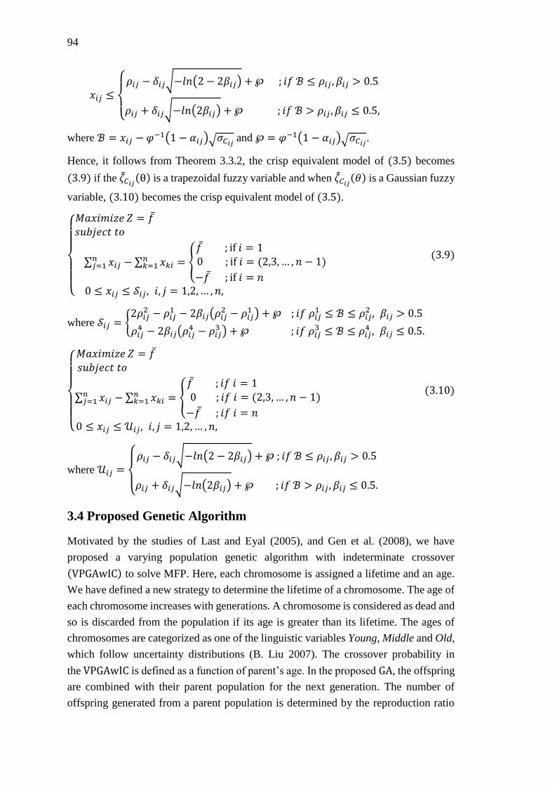
94

𝑥𝑖𝑗 ≤

{


𝜌𝑖𝑗 + 𝛿𝑖𝑗√−𝑙𝑛(2𝛽𝑖𝑗) + ℘ ; 𝑖𝑓 ℬ > 𝜌𝑖𝑗 , 𝛽𝑖𝑗 ≤ 0.5,

where ℬ = 𝑥𝑖𝑗 −𝜑−1(1 − 𝛼𝑖𝑗)√𝜎𝐶𝑖𝑗 and ℘ = 𝜑−1(1 − 𝛼𝑖𝑗)√𝜎𝐶𝑖𝑗.

Hence, it follows from Theorem 3.3.2, the crisp equivalent model of (3.5) becomes

(3.9) if the 휁𝐶𝑖𝑗(θ) is a trapezoidal fuzzy variable and when 휁𝐶𝑖𝑗(휃) is a Gaussian fuzzy

variable, (3.10) becomes the crisp equivalent model of (3.5).

{



𝑛𝑘=1 = {

𝑓 ; if 𝑖 = 1

0 ; if 𝑖 = (2,3, … , 𝑛 − 1)

−𝑓 ; if 𝑖 = 𝑛 0 ≤ 𝑥𝑖𝑗 ≤ 𝒮𝑖𝑗 , 𝑖, 𝑗 = 1,2, … , 𝑛,

(3.9)

where 𝒮𝑖𝑗 = {2𝜌𝑖𝑗


2 − 𝜌𝑖𝑗1 ) + ℘ ; 𝑖𝑓 𝜌𝑖𝑗

1 ≤ ℬ ≤ 𝜌𝑖𝑗2 , 𝛽𝑖𝑗 > 0.5


4 − 𝜌𝑖𝑗3 ) + ℘ ; 𝑖𝑓 𝜌𝑖𝑗

3 ≤ ℬ ≤ 𝜌𝑖𝑗4 , 𝛽𝑖𝑗 ≤ 0.5.

{



𝑛𝑘=1 = {

𝑓 ; 𝑖𝑓 𝑖 = 1 0 ; 𝑖𝑓 𝑖 = (2,3, … , 𝑛 − 1)

−𝑓 ; 𝑖𝑓 𝑖 = 𝑛 0 ≤ 𝑥𝑖𝑗 ≤ 𝒰𝑖𝑗, 𝑖, 𝑗 = 1,2, … , 𝑛,

(3.10)

where 𝒰𝑖𝑗 =

{


𝜌𝑖𝑗 + 𝛿𝑖𝑗√−𝑙𝑛(2𝛽𝑖𝑗) + ℘ ; 𝑖𝑓 ℬ > 𝜌𝑖𝑗 , 𝛽𝑖𝑗 ≤ 0.5.

3.4 Proposed Genetic Algorithm

Motivated by the studies of Last and Eyal (2005), and Gen et al. (2008), we have

proposed a varying population genetic algorithm with indeterminate crossover

(VPGAwIC) to solve MFP. Here, each chromosome is assigned a lifetime and an age.

We have defined a new strategy to determine the lifetime of a chromosome. The age of

each chromosome increases with generations. A chromosome is considered as dead and

so is discarded from the population if its age is greater than its lifetime. The ages of

chromosomes are categorized as one of the linguistic variables Young, Middle and Old,

which follow uncertainty distributions (B. Liu 2007). The crossover probability in

the VPGAwIC is defined as a function of parent’s age. In the proposed GA, the offspring

are combined with their parent population for the next generation. The number of

offspring generated from a parent population is determined by the reproduction ratio

95

(Z. Michalewicz 1992). In a particular generation, the total population size does not

exceed a predetermined threshold.

To describe the proposed algorithm VPGAwIC, the following notations are used.

𝑇: Generation count

𝑎𝑔𝑒: Age of a chromosome in terms to 𝑇

𝑙𝑖𝑓𝑒𝑡𝑖𝑚𝑒: Maximum age, a chromosome can stay alive in terms of 𝑇

𝑃𝑜𝑝(𝑇): Population at generation 𝑇

𝐶(𝑇): Offspring population generated by 𝑃𝑜𝑝(𝑇)

𝐷𝑒𝑎𝑑(𝑇): Set of chromosomes from 𝑃𝑜𝑝(𝑇), whose 𝑎𝑔𝑒 > 𝑙𝑖𝑓𝑒𝑡𝑖𝑚𝑒

𝑔𝑚𝑎𝑥: Maximum generation number

𝜌: Reproduction ratio

𝜉𝑝𝑐: Uncertain crossover probability

𝑝𝑚: Mutation probability

𝑃𝑜𝑝𝑆𝑖𝑧𝑒𝑇ℎ: Maximum number of chromosomes in a generation

𝑀𝑎𝑥𝑓𝑖𝑡𝑇: Maximum fitness of population at 𝑇𝑡ℎ generation

𝑀𝑖𝑛𝑓𝑖𝑡𝑇: Minimum fitness of population at 𝑇𝑡ℎ generation

𝐴𝑣𝑔𝑓𝑖𝑡𝑇: Average fitness value of population at 𝑇𝑡ℎ generation

𝑀𝑎𝑥𝑆𝑎𝑚𝑒𝐶𝑜𝑢𝑛𝑡: Maximum allowed number of consecutive generations with

same 𝐴𝑣𝑔𝑓𝑖𝑡𝑇

𝐶𝑃: Permissible flow of a network path 𝑃

𝑐𝑖𝑗: Maximum capacity of an edge

𝐹𝑅: Fitness value of a chromosome 𝑅 (maximum flow of a chromosome)

𝐶𝑀{𝑐𝑚𝑖𝑗, 𝑖, 𝑗 = 1,2, … , 𝑛}: Capacity matrix of a network, where each element

𝑐𝑚𝑖𝑗 represents the capacity of an edge 𝑒𝑖𝑗

𝐿𝑖: Set of nodes adjacent to node 𝑣𝑖

𝑉𝑖𝑠𝑖𝑡𝑒𝑑𝑚: Determine whether a node 𝑣𝑚 is included in a path 𝑃,

i.e., 𝑉𝑖𝑠𝑖𝑡𝑒𝑑𝑚 = {𝑡𝑟𝑢𝑒 ; if visited, i. e., 𝑣𝑚 ∈ 𝑃 𝑓𝑎𝑙𝑠𝑒 ; if not visited, i. e., 𝑣𝑚 ∉ 𝑃

𝑠: Source node of the network

𝑡: Sink node of the network

𝐿𝑒𝑛: Current length of the generated path 𝑃

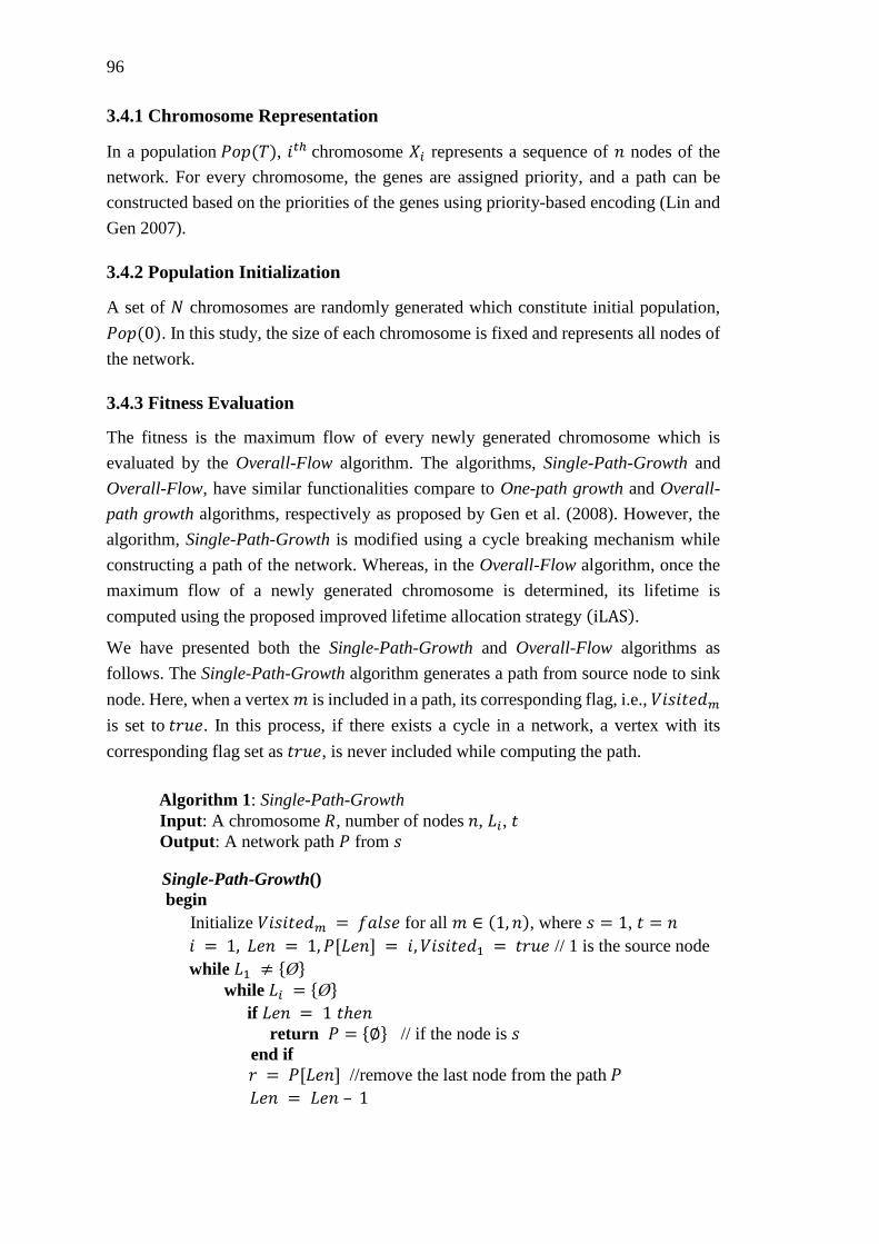
96

3.4.1 Chromosome Representation

In a population 𝑃𝑜𝑝(𝑇), 𝑖𝑡ℎ chromosome 𝑋𝑖 represents a sequence of 𝑛 nodes of the

network. For every chromosome, the genes are assigned priority, and a path can be

constructed based on the priorities of the genes using priority-based encoding (Lin and

Gen 2007).

3.4.2 Population Initialization

A set of 𝑁 chromosomes are randomly generated which constitute initial population,

𝑃𝑜𝑝(0). In this study, the size of each chromosome is fixed and represents all nodes of

the network.

3.4.3 Fitness Evaluation

The fitness is the maximum flow of every newly generated chromosome which is

evaluated by the Overall-Flow algorithm. The algorithms, Single-Path-Growth and

Overall-Flow, have similar functionalities compare to One-path growth and Overall-

path growth algorithms, respectively as proposed by Gen et al. (2008). However, the

algorithm, Single-Path-Growth is modified using a cycle breaking mechanism while

constructing a path of the network. Whereas, in the Overall-Flow algorithm, once the

maximum flow of a newly generated chromosome is determined, its lifetime is

computed using the proposed improved lifetime allocation strategy (iLAS).

We have presented both the Single-Path-Growth and Overall-Flow algorithms as

follows. The Single-Path-Growth algorithm generates a path from source node to sink

node. Here, when a vertex 𝑚 is included in a path, its corresponding flag, i.e., 𝑉𝑖𝑠𝑖𝑡𝑒𝑑𝑚

is set to 𝑡𝑟𝑢𝑒. In this process, if there exists a cycle in a network, a vertex with its

corresponding flag set as 𝑡𝑟𝑢𝑒, is never included while computing the path.

Algorithm 1: Single-Path-Growth

Input: A chromosome 𝑅, number of nodes 𝑛, 𝐿𝑖, 𝑡 Output: A network path 𝑃 from 𝑠

Single-Path-Growth()

begin

Initialize 𝑉𝑖𝑠𝑖𝑡𝑒𝑑𝑚 = 𝑓𝑎𝑙𝑠𝑒 for all 𝑚 ∈ (1, 𝑛), where 𝑠 = 1, 𝑡 = 𝑛

𝑖 = 1, 𝐿𝑒𝑛 = 1, 𝑃[𝐿𝑒𝑛] = 𝑖, 𝑉𝑖𝑠𝑖𝑡𝑒𝑑1 = 𝑡𝑟𝑢𝑒 // 1 is the source node

while 𝐿1 ≠ {Ø} while 𝐿𝑖 = {Ø}

if 𝐿𝑒𝑛 = 1 𝑡ℎ𝑒𝑛

return 𝑃 = {∅} // if the node is 𝑠 end if

𝑟 = 𝑃[𝐿𝑒𝑛] //remove the last node from the path 𝑃

𝐿𝑒𝑛 = 𝐿𝑒𝑛 – 1

97

𝑅[𝑟] = 0 // set the priority of the removed node to 0 so that it

//is not selected again if an intermediate node has no outgoing

//edges from it.

if 𝐿𝑒𝑛 > 1 then 𝑖 = 𝑃[𝐿𝑒𝑛] else

return 𝑃 // if the node is 𝑡 end if

end while

Set 𝑗 ′ = 0

𝑗 ′ = node with highest priority among non-visited nodes of 𝐿𝑖 if 𝑗 ′ > 0 𝑎𝑛𝑑 𝑅[𝑗 ′] ≠ 0

𝐿𝑒𝑛 = 𝐿𝑒𝑛 + 1, 𝑃[𝐿𝑒𝑛] = 𝑗 ′, 𝑖 = 𝑗 ′ // Add 𝑖 to path and

//make 𝑖 to 𝑗 ′

𝑉𝑖𝑠𝑖𝑡𝑒𝑑𝑗′ = 𝑡𝑟𝑢𝑒

else

𝑟 = 𝑃[𝐿𝑒𝑛], 𝐿𝑒𝑛 = 𝐿𝑒𝑛 − 1

𝑉𝑖𝑠𝑖𝑡𝑒𝑑𝑟 = 𝑡𝑟𝑢𝑒

if 𝐿𝑒𝑛 > 1 𝑡ℎ𝑒𝑛

𝑖 = 𝑃[𝐿𝑒𝑛] end if

end if

if 𝑃[L𝑒𝑛] = 𝑡 then

return 𝑃 end if

end while

end

Algorithm 2: Overall-Flow

Input: Capacity matrix (𝐶𝑀 = {𝑐𝑚𝑖𝑗, 𝑖, 𝑗 = 1,2, … , 𝑛}), adjacent list of 𝑖𝑡ℎ node 𝐿𝑖,

population 𝑃𝑜𝑝(𝑇), source node 𝑠, destination node 𝑡 Output: Determine 𝐹𝑅, 𝑙𝑖𝑓𝑒𝑡𝑖𝑚𝑒 of each chromosome 𝑅 in 𝑃𝑜𝑝(𝑇)

Overall-Flow()

begin

for each chromosome 𝑅 in 𝑃𝑜𝑝(𝑇) if 𝐹𝑅 = −1 then

Set 𝑎𝑔𝑒=0

while 𝐿1 ≠ {∅} // 𝐿1 represents the source node 𝑠.

𝑃= Single-Path-Growth () // Evaluate path 𝑃 and determine the

//sink node 𝑎 of 𝑃

if 𝑎 = 𝑡 then

𝐶𝑝= min{𝑐𝑚𝑖𝑗|𝑒𝑖𝑗 ∈ 𝑃}

𝐹𝑅 = 𝐹𝑅 + 𝐶𝑝

98

𝑐𝑚𝑖𝑗 = {𝑐𝑚𝑖𝑗 − 𝐶𝑝 ; 𝑖𝑓 𝑒𝑖𝑗 ∈ 𝑃

𝑐𝑚𝑖𝑗 ; 𝑜𝑡ℎ𝑒𝑟𝑤𝑖𝑠𝑒

if 𝑐𝑚𝑖𝑗 = 0 then

𝐿𝑖 = 𝐿𝑖\𝑣𝑗

end if

else

𝐿𝑖 = 𝐿𝑖\𝑎 ∀ 𝑖 ∈ {1,2, … , 𝑛} // update the set of nodes in 𝐿𝑖

end if

end while

end if

end for

Compute 𝑀𝑎𝑥𝑓𝑖𝑡𝑇, 𝐴𝑣𝑔𝑓𝑖𝑡𝑇 and 𝑀𝑖𝑛𝑓𝑖𝑡𝑇 for 𝑃𝑜𝑝(𝑇)

Compute 𝑙𝑖𝑓𝑒𝑡𝑖𝑚𝑒 to every newly generated chromosome by iLAS.

end

3.4.4 Age and Lifetime of Chromosome

In a generation, the age of a newly born chromosome 𝑋𝑖 is initialized to zero and its

lifetime is computed following the proposed improved lifetime allocation

strategy (iLAS), which is a modified version of the bilinear allocation strategy (bLAS)

(Z. Michalewicz 1992). The iLAS is defined below in (3.11).

𝑙𝑖𝑓𝑒𝑡𝑖𝑚𝑒(𝑋𝑖)

=

{

𝑚𝑖𝑛𝐿𝑇 + 𝜅

𝐹𝑋𝑖 −𝑀𝑖𝑛𝑓𝑖𝑡𝑇

𝐴𝑣𝑔𝑓𝑖𝑡𝑇 −𝑀𝑖𝑛𝑓𝑖𝑡𝑇 ; 𝑖𝑓 𝐴𝑣𝑔𝑓𝑖𝑡𝑇 ≥ 𝐹𝑋𝑖

1

2(𝑚𝑖𝑛𝐿𝑇 +𝑚𝑎𝑥𝐿𝑇) + 𝜅

𝐹𝑋𝑖 +𝑀𝑎𝑥𝑓𝑖𝑡𝑇 − (2 ∗ 𝐴𝑣𝑔𝑓𝑖𝑡𝑇)

2 ∗ (𝑀𝑎𝑥𝑓𝑖𝑡𝑇 − 𝐴𝑣𝑔𝑓𝑖𝑡𝑇) ; 𝑜𝑡ℎ𝑒𝑟𝑤𝑖𝑠𝑒,

(3.11)

where

𝐹𝑋𝑖: Fitness value of a chromosome (solution) of 𝑋𝑖

𝑚𝑎𝑥𝐿𝑇: Maximum lifetime of a chromosome

𝑚𝑖𝑛𝐿𝑇: Minimum lifetime of a chromosome

𝜅 =1

2(𝑚𝑎𝑥𝐿𝑇 −𝑚𝑖𝑛𝐿𝑇) (3.12)

The age of a chromosome increases by one with generation. Once the age of a

chromosome exceeds its lifetime, the chromosome is considered as dead. A

chromosome is 𝑌𝑜𝑢𝑛𝑔, 𝑀𝑖𝑑𝑑𝑙𝑒 or 𝑂𝑙𝑑 according to its age. In this study, the linguistic

variables associated with the age of chromosomes are uncertain variables (B. Liu 2007),

whose uncertainty distributions are depicted in Fig. 3.1. Here, 𝑌𝑜𝑢𝑛𝑔 and 𝑂𝑙𝑑 are

99

represented by linear uncertainty distribution, whereas 𝑀𝑖𝑑𝑑𝑙𝑒 is represented by zigzag

uncertainty distribution (cf. definitions 1.3.29 and 1.3.30 of Section 1.3.11).

Figure 3.1 Uncertainty distributions of chromosome’s age

The average of the lifetimes of the chromosomes is the average lifetime of the

corresponding population. Subsequently, the 𝑟𝑒𝑙𝑎𝑡𝑖𝑣𝑒 𝑎𝑔𝑒 of a chromosome is defined

as the ratio between its age and an average lifetime of the corresponding population.

Thereafter, the relative ages of the chromosomes are normalized, and the age interval

of a chromosome 𝑋𝑖 is essentially determined as an uncertain variable, which is

categorized as 𝑌𝑜𝑢𝑛𝑔, 𝑀𝑖𝑑𝑑𝑙𝑒 or 𝑂𝑙𝑑. In particular, the age interval for 𝑌𝑜𝑢𝑛𝑔 and

𝑂𝑙𝑑 are linear uncertain variables and represented by ℒ(0, 0.275) and ℒ(0.650, 1.0),

respectively. Whereas, 𝑀𝑖𝑑𝑑𝑙𝑒 in represented by a zigzag uncertain

variable 𝒵(0.225, 0.350, 0.675).

3.4.5 Crossover

Crossover between two chromosomes, 𝑋𝑖 and 𝑋𝑗 is performed by following the steps as

discussed below.

(i) Crossover probability (𝜉𝑝𝑐): Once the age intervals of the parents 𝑋𝑖 and 𝑋𝑗

are identified, the corresponding crossover probability 𝜉𝑝𝑐 is estimated as an

uncertain variable (i.e., 𝐿, 𝑀 or 𝐻) using the uncertain rule base as reported in Table

3.1. Here, 𝐿, 𝑀 and 𝐻, respectively represents 𝐿𝑜𝑤, 𝑀𝑒𝑑𝑖𝑢𝑚 and 𝐻𝑖𝑔ℎ. In other

words, the indeterminacy in the crossover probability for a pair of chromosomes

(𝑋𝑖, 𝑋𝑗) can be either 𝐿𝑜𝑤, 𝑀𝑒𝑑𝑖𝑢𝑚 or 𝐻𝑖𝑔ℎ based on the age intervals of 𝑋𝑖

and 𝑋𝑗. Here, we have considered 𝐿 and 𝐻 as linear uncertain variables which are

respectively, ℒ(0, 0.250) and ℒ(0.70,1.0). Whereas, 𝑀 is a zigzag uncertain

variable represented by 𝒵(0.150, 0.350, 0.750). Uncertainty distributions of 𝐿, 𝑀

and 𝐻 are depicted in Fig. 3.2.

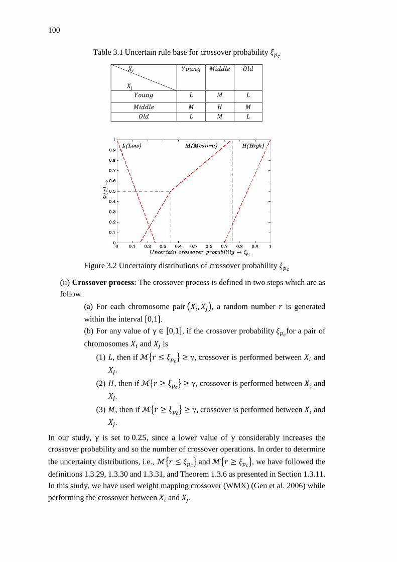
100

Table 3.1 Uncertain rule base for crossover probability 𝜉𝑝𝑐

𝑋𝑖

𝑋𝑗

𝑌𝑜𝑢𝑛𝑔 𝑀𝑖𝑑𝑑𝑙𝑒 𝑂𝑙𝑑

𝑌𝑜𝑢𝑛𝑔 𝐿 𝑀 𝐿

𝑀𝑖𝑑𝑑𝑙𝑒 𝑀 𝐻 𝑀

𝑂𝑙𝑑 𝐿 𝑀 𝐿

Figure 3.2 Uncertainty distributions of crossover probability 𝜉𝑝𝑐

(ii) Crossover process: The crossover process is defined in two steps which are as

follow.

(a) For each chromosome pair (𝑋𝑖, 𝑋𝑗), a random number 𝑟 is generated

within the interval [0,1].

(b) For any value of γ ∈ [0,1], if the crossover probability 𝜉𝑝𝑐for a pair of

chromosomes 𝑋𝑖 and 𝑋𝑗 is

(1) 𝐿, then if ℳ{𝑟 ≤ 𝜉𝑝𝑐} ≥ γ, crossover is performed between 𝑋𝑖 and

𝑋𝑗.

(2) 𝐻, then if ℳ{𝑟 ≥ 𝜉𝑝𝑐} ≥ γ, crossover is performed between 𝑋𝑖 and

𝑋𝑗.

(3) 𝑀, then if ℳ{𝑟 ≥ 𝜉𝑝𝑐} ≥ γ, crossover is performed between 𝑋𝑖 and

𝑋𝑗.

In our study, γ is set to 0.25, since a lower value of γ considerably increases the

crossover probability and so the number of crossover operations. In order to determine

the uncertainty distributions, i.e., ℳ{𝑟 ≤ 𝜉𝑝𝑐} and ℳ{𝑟 ≥ 𝜉𝑝𝑐}, we have followed the

definitions 1.3.29, 1.3.30 and 1.3.31, and Theorem 1.3.6 as presented in Section 1.3.11.

In this study, we have used weight mapping crossover (WMX) (Gen et al. 2006) while

performing the crossover between 𝑋𝑖 and 𝑋𝑗.

101

3.4.6 Mutation

Mutation is performed based on mutation probability 𝑝𝑚. For this purpose, a random

number 𝑞 within the range [0,1] is generated. If 𝑞 < 𝑝𝑚, then the mutation is

performed. Here, we have used insertion mutation (Gen et al. 2008) in VPGAwIC.

3.4.7 Selection

After crossover and mutation are performed on parent population 𝑃𝑜𝑝(𝑇), a total of

⌊𝜌 ∗ |𝑃𝑜𝑝(𝑇)|⌋ individuals are generated in the offspring population 𝐶(𝑇), where ρ is

the reproduction ratio (Z. Michalewicz 1992). In parent population, those solutions with

ages greater than their lifetimes are considered as dead and are rejected. Thus

{𝑃𝑜𝑝(𝑇) − 𝐷𝑒𝑎𝑑(𝑇)} ∪ 𝐶(𝑇) along with two elitist solutions are used for next

generation 𝑃𝑜𝑝(𝑇 + 1). If the population size at 𝑃𝑜𝑝(𝑇 + 1) is greater

than 𝑃𝑜𝑝𝑆𝑖𝑧𝑒𝑇ℎ, we randomly eliminate some chromosomes from 𝑃𝑜𝑝(𝑇 + 1) to

maintain its size. However, this process ensures that the elitist solutions are preserved

in 𝑃𝑜𝑝(𝑇 + 1).

3.4.8 Elitist Selection

From the parent population 𝑃𝑜𝑝(𝑇), two best solutions are selected for crossover to

generate their offspring. This confirms that even if the best solutions in 𝑃𝑜𝑝(𝑇) die

in 𝑃𝑜𝑝(𝑇 + 1), their offspring are preserved in the next generation.

3.4.9 Stopping Criteria

The execution of the algorithm terminates when either or both the following two

conditions are satisfied.

(i) Number of generations reaches 𝑔𝑚𝑎𝑥.

(ii) Number of generations giving the same average fitness values

reaches, 𝑀𝑎𝑥𝑆𝑎𝑚𝑒𝐶𝑜𝑢𝑛𝑡.

Algorithm 3: VPGAwIC

Input: 𝑉, 𝐸 and the capacities associated with all the edges of the given network

Output: Maximum flow of the network 𝐺

𝑽𝑷𝑮𝑨𝒘𝑰𝑪( )

begin

Set 𝑇 = 0, 𝑆𝑎𝑚𝑒𝐶𝑜𝑢𝑛𝑡=0

Generate initial population 𝑃𝑜𝑝(𝑇) by priority based encoding

for each chromosome 𝑅, 𝐹𝑅 = −1 in 𝑃𝑜𝑝(𝑇)

Execute Overall-Flow on 𝑃𝑜𝑝(𝑇) // Determine the maximum flow and

lifetime of every newly generated chromosome in 𝑃𝑜𝑝(𝑇).

102

while 𝑆𝑎𝑚𝑒𝐶𝑜𝑢𝑛𝑡 < 𝑀𝑎𝑥𝑆𝑎𝑚𝑒𝐶𝑜𝑢𝑛𝑡 AND 𝑇 < 𝑔𝑚𝑎𝑥

Determine the normalize relative age for each chromosome in 𝑃𝑜𝑝(𝑇)

Set 𝐶(𝑇) = {∅}

Select two best solutions from 𝑃𝑜𝑝(𝑇), perform WMX crossover on

them and insert their offspring to 𝐶(𝑇).

if ((|𝐶(𝑇)| + |𝑃𝑜𝑝(𝑇)|) ≤ 𝑃𝑜𝑝𝑆𝑖𝑧𝑒𝑇ℎ)

Determine uncertain crossover probability 𝜉𝑝𝑐 for

each selected pair of parents from 𝑃𝑜𝑝(𝑇).

Generate offspring by performing WMX crossover with

probability 𝜉𝑝𝑐

For each offspring, perform insertion mutation with probability 𝑝𝑚

Add newly generated offspring to 𝐶(𝑇)

end if

Set 𝐷𝑒𝑎𝑑(𝑇) = {∅}

For each chromosome in 𝐶(𝑇) set 𝐹𝑅 = −1.

Increment age of each chromosome by 1 in 𝑃𝑜𝑝(𝑇).

Construct 𝐷𝑒𝑎𝑑(𝑇) if 𝑎𝑔𝑒 > 𝑙𝑖𝑓𝑒𝑡𝑖𝑚𝑒 for all chromosomes

of 𝑃𝑜𝑝(𝑇). //Find the set of dead chromosomes

𝑃𝑜𝑝(𝑇 + 1) = {𝑃𝑜𝑝(𝑇) − 𝐷𝑒𝑎𝑑(𝑇)} ∪ 𝐶(𝑇).

Execute Overall-Flow() on 𝑃𝑜𝑝(𝑇 + 1). // Determine the maximum

flow and lifetime of every newly generated chromosome in 𝑃𝑜𝑝(𝑇 + 1).

if 𝐴𝑣𝑔𝑓𝑖𝑡𝑇+1 = 𝐴𝑣𝑔𝑓𝑖𝑡𝑇 𝑡ℎ𝑒𝑛

𝑆𝑎𝑚𝑒𝐶𝑜𝑢𝑛t= 𝑆𝑎𝑚𝑒𝐶𝑜𝑢𝑛t +1

else

𝑆𝑎𝑚𝑒𝐶𝑜𝑢𝑛t = 0

end if

𝑇 = 𝑇 + 1

end while

Return best chromosome of 𝑃𝑜𝑝(𝑇)

end

3.5 Results and Discussion

The performance of the proposed VPGAwIC is tested using six crisp instances of the

maximum flow problem. Those maximum flow instances are named as 𝑚𝑓𝑙𝑜𝑤_𝑣_𝑒,

where 𝑣 and 𝑒 are the number of nodes and edges, respectively. For each of these

instances, the results of the proposed algorithm, VPGAwIC are compared with the

genetic algorithm (GA) proposed by Gen et al. (2008). For comparison purpose, we

have renamed the GA of Gen et al. (2008) as maximum flow genetic algorithm (MFGA).

103

The platform we have used for simulation is a personal computer with Intel (𝑅)

Core(𝑇𝑀) i3 @ 2.93GHz and 4 GB memory. In Section 3.5.1, the results generated by

the algorithms, for the crisp instances are compared. Out of the six maximum flow

instances, the description of 𝑚𝑓𝑙𝑜𝑤_11_22 and 𝑚𝑓𝑙𝑜𝑤_25_49 are given by Gen et al.

(2008). The instance 𝑚𝑓𝑙𝑜𝑤_20_300 is taken from the location:

ftp://dimacs.rutgers.edu/pub/netflow/maxflow/solver-4 which is defined in the

file 𝑤𝑤.𝑚𝑎𝑥. While, the instances 𝑚𝑓𝑙𝑜𝑤_102_290, 𝑚𝑓𝑙𝑜𝑤_902_2670 and

𝑚𝑓𝑙𝑜𝑤_2502_7450 are accessed from the location

ftp://dimacs.rutgers.edu/pub/netflow/maxflow/solver-3. These instances are

maintained, respectively in the files, 𝑚10.𝑚𝑎𝑥, 𝑚30.𝑚𝑎𝑥 and 𝑚50.𝑚𝑎𝑥. While

executing the MFGA on 𝑚𝑓𝑙𝑜𝑤_20_300, Single-Path-Growth mechanism is used

instead of One-path growth (Gen et al. 2008). In 𝑚𝑓𝑙𝑜𝑤_20_300 there exist cycles,

and so a path from source to destination cannot be constructed if One-path growth is

incorporated with the MFGA. In this section, the better experimental results in the tables

are shown in bold. In Section 3.5.2, the results of the VPGAwIC are presented for the

crisp equivalents of the EVM and the CCM for the random fuzzy maximum flow

problem. These results are then compared with that generated by LINGO 11.0. Finally,

a sensitivity analysis is also presented by executing the VPGAwIC at different

confidence levels, for the crisp equivalent of the CCM of RFMFP.

3.5.1 Crisp Instances

In this subsection, the experimental results of the MFGA and the proposed VPGAwIC

are compared for six maximum flow instances. The parameter setting for

experimentation of MFGA and VPGAwIC are presented in Table 3.2. For VPGAwIC, the

initial population size is set to 50, and at subsequent generations, the population varies

with a maximum threshold (𝑃𝑜𝑝𝑆𝑖𝑧𝑒𝑇ℎ) of 5000.

Due to stochastic nature of the algorithms considered in this chapter, to compare the

performances of the existing MFGA and the proposed VPGAwIC, the present study

considers 50 runs for each of the algorithms on every instance. We have computed the

values, 𝑚𝑎𝑥 𝑓𝑖𝑡𝑛𝑒𝑠𝑠, 𝑚𝑒𝑎𝑛 𝑓𝑖𝑡𝑛𝑒𝑠𝑠 with standard deviation (𝑠𝑑) and 𝑚𝑒𝑎𝑛

𝑒𝑥𝑒𝑐𝑢𝑡𝑖𝑜𝑛 𝑡𝑖𝑚𝑒 in milliseconds (𝑚𝑠) for all the instances. These results are reported

in Table 3.3, where it is observed that for the instances, 𝑚𝑓𝑙𝑜𝑤_11_22,

𝑚𝑓𝑙𝑜𝑤_25_49 and 𝑚𝑓𝑙𝑜𝑤_20_300, 𝑚𝑎𝑥 𝑓𝑖𝑡𝑛𝑒𝑠𝑠 and 𝑚𝑒𝑎𝑛 𝑓𝑖𝑡𝑛𝑒𝑠𝑠 (after 50 runs

of the algorithm) do not differ for both the MFGA and VPGAwIC. Therefore, the values

of 𝑠𝑑 for these instances are zero. However, for the maximum flow

instances, 𝑚𝑓𝑙𝑜𝑤_102_290, 𝑚𝑓𝑙𝑜𝑤_902_2670 and 𝑚𝑓𝑙𝑜𝑤_2502_7450,

𝑚𝑎𝑥 𝑓𝑖𝑡𝑛𝑒𝑠𝑠 and 𝑚𝑒𝑎𝑛 𝑓𝑖𝑡𝑛𝑒𝑠𝑠 are better in case of the VPGAwIC as compare to the

MFGA.

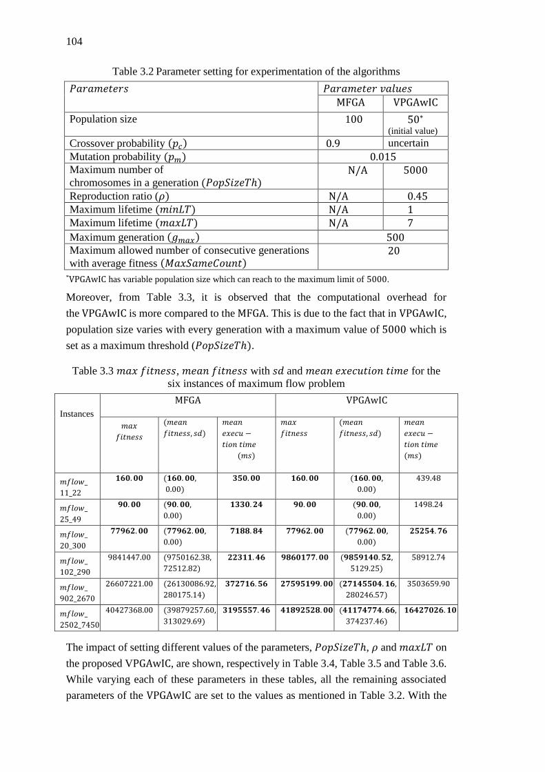
ftp://dimacs.rutgers.edu/pub/netflow/maxflow/solver-4

ftp://dimacs.rutgers.edu/pub/netflow/maxflow/solver-3

104

Table 3.2 Parameter setting for experimentation of the algorithms

𝑃𝑎𝑟𝑎𝑚𝑒𝑡𝑒𝑟𝑠 𝑃𝑎𝑟𝑎𝑚𝑒𝑡𝑒𝑟 𝑣𝑎𝑙𝑢𝑒𝑠 MFGA VPGAwIC

Population size 100 50∗ (initial value)

Crossover probability (𝑝𝑐) 0.9 uncertain

Mutation probability (𝑝𝑚) 0.015

Maximum number of

chromosomes in a generation (𝑃𝑜𝑝𝑆𝑖𝑧𝑒𝑇ℎ) N/A 5000

Reproduction ratio (𝜌) N/A 0.45 Maximum lifetime (𝑚𝑖𝑛𝐿𝑇) N/A 1

Maximum lifetime (𝑚𝑎𝑥𝐿𝑇) N/A 7

Maximum generation (𝑔𝑚𝑎𝑥) 500

Maximum allowed number of consecutive generations

with average fitness (𝑀𝑎𝑥𝑆𝑎𝑚𝑒𝐶𝑜𝑢𝑛𝑡) 20

*VPGAwIC has variable population size which can reach to the maximum limit of 5000.

Moreover, from Table 3.3, it is observed that the computational overhead for

the VPGAwIC is more compared to the MFGA. This is due to the fact that in VPGAwIC,

population size varies with every generation with a maximum value of 5000 which is

set as a maximum threshold (𝑃𝑜𝑝𝑆𝑖𝑧𝑒𝑇ℎ).

Table 3.3 𝑚𝑎𝑥 𝑓𝑖𝑡𝑛𝑒𝑠𝑠, 𝑚𝑒𝑎𝑛 𝑓𝑖𝑡𝑛𝑒𝑠𝑠 with 𝑠𝑑 and 𝑚𝑒𝑎𝑛 𝑒𝑥𝑒𝑐𝑢𝑡𝑖𝑜𝑛 𝑡𝑖𝑚𝑒 for the

six instances of maximum flow problem

Instances

MFGA VPGAwIC

𝑚𝑎𝑥

𝑓𝑖𝑡𝑛𝑒𝑠𝑠

(𝑚𝑒𝑎𝑛

𝑓𝑖𝑡𝑛𝑒𝑠𝑠, 𝑠𝑑)

𝑚𝑒𝑎𝑛

𝑒𝑥𝑒𝑐𝑢 −

𝑡𝑖𝑜𝑛 𝑡𝑖𝑚𝑒

(𝑚𝑠)

𝑚𝑎𝑥


(𝑚𝑒𝑎𝑛


𝑚𝑒𝑎𝑛



(𝑚𝑠)

𝑚𝑓𝑙𝑜𝑤_

11_22

𝟏𝟔𝟎. 𝟎𝟎 (𝟏𝟔𝟎. 𝟎𝟎,

0.00)

𝟑𝟓𝟎. 𝟎𝟎 𝟏𝟔𝟎. 𝟎𝟎 (𝟏𝟔𝟎. 𝟎𝟎,

0.00)

439.48


25_49

𝟗𝟎. 𝟎𝟎 (𝟗𝟎. 𝟎𝟎,

0.00)

𝟏𝟑𝟑𝟎. 𝟐𝟒 𝟗𝟎. 𝟎𝟎 (𝟗𝟎. 𝟎𝟎,

0.00)

1498.24


20_300

𝟕𝟕𝟗𝟔𝟐. 𝟎𝟎 (𝟕𝟕𝟗𝟔𝟐. 𝟎𝟎,

0.00)

𝟕𝟏𝟖𝟖. 𝟖𝟒 𝟕𝟕𝟗𝟔𝟐. 𝟎𝟎 (𝟕𝟕𝟗𝟔𝟐. 𝟎𝟎,

0.00)

𝟐𝟓𝟐𝟓𝟒. 𝟕𝟔


102_290

9841447.00 (9750162.38,

72512.82)

𝟐𝟐𝟑𝟏𝟏. 𝟒𝟔 𝟗𝟖𝟔𝟎𝟏𝟕𝟕. 𝟎𝟎 (𝟗𝟖𝟓𝟗𝟏𝟒𝟎. 𝟓𝟐,

5129.25)

58912.74


902_2670

26607221.00 (26130086.92,

280175.14)

𝟑𝟕𝟐𝟕𝟏𝟔. 𝟓𝟔 𝟐𝟕𝟓𝟗𝟓𝟏𝟗𝟗. 𝟎𝟎 (𝟐𝟕𝟏𝟒𝟓𝟓𝟎𝟒. 𝟏𝟔,

280246.57)

3503659.90


2502_7450

40427368.00 (39879257.60,

313029.69)

𝟑𝟏𝟗𝟓𝟓𝟓𝟕. 𝟒𝟔 𝟒𝟏𝟖𝟗𝟐𝟓𝟐𝟖. 𝟎𝟎 (𝟒𝟏𝟏𝟕𝟒𝟕𝟕𝟒. 𝟔𝟔,

374237.46)

𝟏𝟔𝟒𝟐𝟕𝟎𝟐𝟔. 𝟏𝟎

The impact of setting different values of the parameters, 𝑃𝑜𝑝𝑆𝑖𝑧𝑒𝑇ℎ, 𝜌 and 𝑚𝑎𝑥𝐿𝑇 on

the proposed VPGAwIC, are shown, respectively in Table 3.4, Table 3.5 and Table 3.6.

While varying each of these parameters in these tables, all the remaining associated

parameters of the VPGAwIC are set to the values as mentioned in Table 3.2. With the

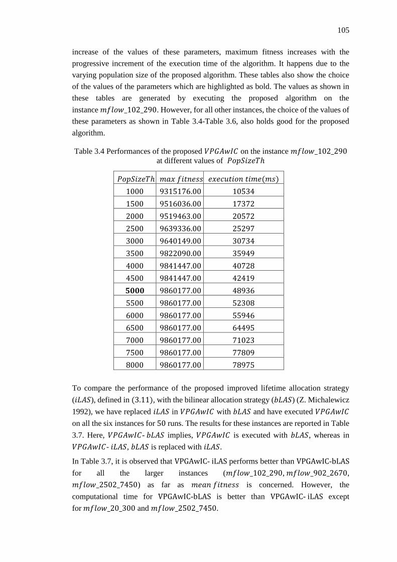
105

increase of the values of these parameters, maximum fitness increases with the

progressive increment of the execution time of the algorithm. It happens due to the

varying population size of the proposed algorithm. These tables also show the choice

of the values of the parameters which are highlighted as bold. The values as shown in

these tables are generated by executing the proposed algorithm on the

instance 𝑚𝑓𝑙𝑜𝑤_102_290. However, for all other instances, the choice of the values of

these parameters as shown in Table 3.4-Table 3.6, also holds good for the proposed

algorithm.

Table 3.4 Performances of the proposed 𝑉𝑃𝐺𝐴𝑤𝐼𝐶 on the instance 𝑚𝑓𝑙𝑜𝑤_102_290

at different values of 𝑃𝑜𝑝𝑆𝑖𝑧𝑒𝑇ℎ

To compare the performance of the proposed improved lifetime allocation strategy

(𝑖𝐿𝐴𝑆), defined in (3.11), with the bilinear allocation strategy (𝑏𝐿𝐴𝑆) (Z. Michalewicz

1992), we have replaced 𝑖𝐿𝐴𝑆 in 𝑉𝑃𝐺𝐴𝑤𝐼𝐶 with 𝑏𝐿𝐴𝑆 and have executed 𝑉𝑃𝐺𝐴𝑤𝐼𝐶

on all the six instances for 50 runs. The results for these instances are reported in Table

3.7. Here, 𝑉𝑃𝐺𝐴𝑤𝐼𝐶- 𝑏𝐿𝐴𝑆 implies, 𝑉𝑃𝐺𝐴𝑤𝐼𝐶 is executed with 𝑏𝐿𝐴𝑆, whereas in

𝑉𝑃𝐺𝐴𝑤𝐼𝐶- 𝑖𝐿𝐴𝑆, 𝑏𝐿𝐴𝑆 is replaced with 𝑖𝐿𝐴𝑆.

In Table 3.7, it is observed that VPGAwIC- iLAS performs better than VPGAwIC-bLAS

for all the larger instances (𝑚𝑓𝑙𝑜𝑤_102_290, 𝑚𝑓𝑙𝑜𝑤_902_2670,

𝑚𝑓𝑙𝑜𝑤_2502_7450) as far as 𝑚𝑒𝑎𝑛 𝑓𝑖𝑡𝑛𝑒𝑠𝑠 is concerned. However, the

computational time for VPGAwIC-bLAS is better than VPGAwIC- iLAS except

for 𝑚𝑓𝑙𝑜𝑤_20_300 and 𝑚𝑓𝑙𝑜𝑤_2502_7450.

𝑃𝑜𝑝𝑆𝑖𝑧𝑒𝑇ℎ 𝑚𝑎𝑥 𝑓𝑖𝑡𝑛𝑒𝑠𝑠 𝑒𝑥𝑒𝑐𝑢𝑡𝑖𝑜𝑛 𝑡𝑖𝑚𝑒(𝑚𝑠)

1000 9315176.00 10534

1500 9516036.00 17372

2000 9519463.00 20572

2500 9639336.00 25297

3000 9640149.00 30734

3500 9822090.00 35949

4000 9841447.00 40728

4500 9841447.00 42419

𝟓𝟎𝟎𝟎 9860177.00 48936

5500 9860177.00 52308

6000 9860177.00 55946

6500 9860177.00 64495

7000 9860177.00 71023

7500 9860177.00 77809

8000 9860177.00 78975

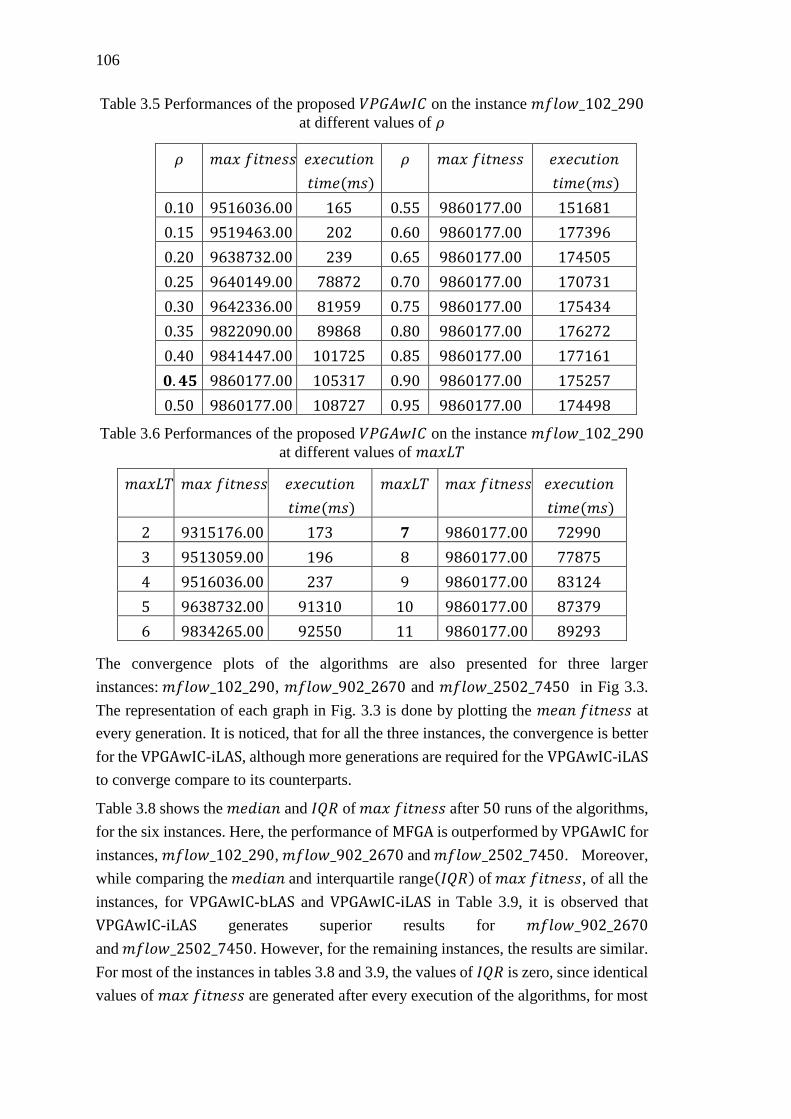
106


at different values of 𝜌


at different values of 𝑚𝑎𝑥𝐿𝑇

The convergence plots of the algorithms are also presented for three larger

instances: 𝑚𝑓𝑙𝑜𝑤_102_290, 𝑚𝑓𝑙𝑜𝑤_902_2670 and 𝑚𝑓𝑙𝑜𝑤_2502_7450 in Fig 3.3.

The representation of each graph in Fig. 3.3 is done by plotting the 𝑚𝑒𝑎𝑛 𝑓𝑖𝑡𝑛𝑒𝑠𝑠 at

every generation. It is noticed, that for all the three instances, the convergence is better

for the VPGAwIC-iLAS, although more generations are required for the VPGAwIC-iLAS

to converge compare to its counterparts.

Table 3.8 shows the 𝑚𝑒𝑑𝑖𝑎𝑛 and 𝐼𝑄𝑅 of 𝑚𝑎𝑥 𝑓𝑖𝑡𝑛𝑒𝑠𝑠 after 50 runs of the algorithms,

for the six instances. Here, the performance of MFGA is outperformed by VPGAwIC for

instances, 𝑚𝑓𝑙𝑜𝑤_102_290, 𝑚𝑓𝑙𝑜𝑤_902_2670 and 𝑚𝑓𝑙𝑜𝑤_2502_7450. Moreover,

while comparing the 𝑚𝑒𝑑𝑖𝑎𝑛 and interquartile range(𝐼𝑄𝑅) of 𝑚𝑎𝑥 𝑓𝑖𝑡𝑛𝑒𝑠𝑠, of all the

instances, for VPGAwIC-bLAS and VPGAwIC-iLAS in Table 3.9, it is observed that

VPGAwIC-iLAS generates superior results for 𝑚𝑓𝑙𝑜𝑤_902_2670

and 𝑚𝑓𝑙𝑜𝑤_2502_7450. However, for the remaining instances, the results are similar.

For most of the instances in tables 3.8 and 3.9, the values of 𝐼𝑄𝑅 is zero, since identical

values of 𝑚𝑎𝑥 𝑓𝑖𝑡𝑛𝑒𝑠𝑠 are generated after every execution of the algorithms, for most

𝜌 𝑚𝑎𝑥 𝑓𝑖𝑡𝑛𝑒𝑠𝑠 𝑒𝑥𝑒𝑐𝑢𝑡𝑖𝑜𝑛

𝑡𝑖𝑚𝑒(𝑚𝑠)

𝜌 𝑚𝑎𝑥 𝑓𝑖𝑡𝑛𝑒𝑠𝑠 𝑒𝑥𝑒𝑐𝑢𝑡𝑖𝑜𝑛


0.10 9516036.00 165 0.55 9860177.00 151681

0.15 9519463.00 202 0.60 9860177.00 177396

0.20 9638732.00 239 0.65 9860177.00 174505

0.25 9640149.00 78872 0.70 9860177.00 170731

0.30 9642336.00 81959 0.75 9860177.00 175434

0.35 9822090.00 89868 0.80 9860177.00 176272

0.40 9841447.00 101725 0.85 9860177.00 177161

𝟎. 𝟒𝟓 9860177.00 105317 0.90 9860177.00 175257

0.50 9860177.00 108727 0.95 9860177.00 174498

𝑚𝑎𝑥𝐿𝑇 𝑚𝑎𝑥 𝑓𝑖𝑡𝑛𝑒𝑠𝑠 𝑒𝑥𝑒𝑐𝑢𝑡𝑖𝑜𝑛


𝑚𝑎𝑥𝐿𝑇 𝑚𝑎𝑥 𝑓𝑖𝑡𝑛𝑒𝑠𝑠 𝑒𝑥𝑒𝑐𝑢𝑡𝑖𝑜𝑛


2 9315176.00 173 𝟕 9860177.00 72990

3 9513059.00 196 8 9860177.00 77875

4 9516036.00 237 9 9860177.00 83124

5 9638732.00 91310 10 9860177.00 87379

6 9834265.00 92550 11 9860177.00 89293

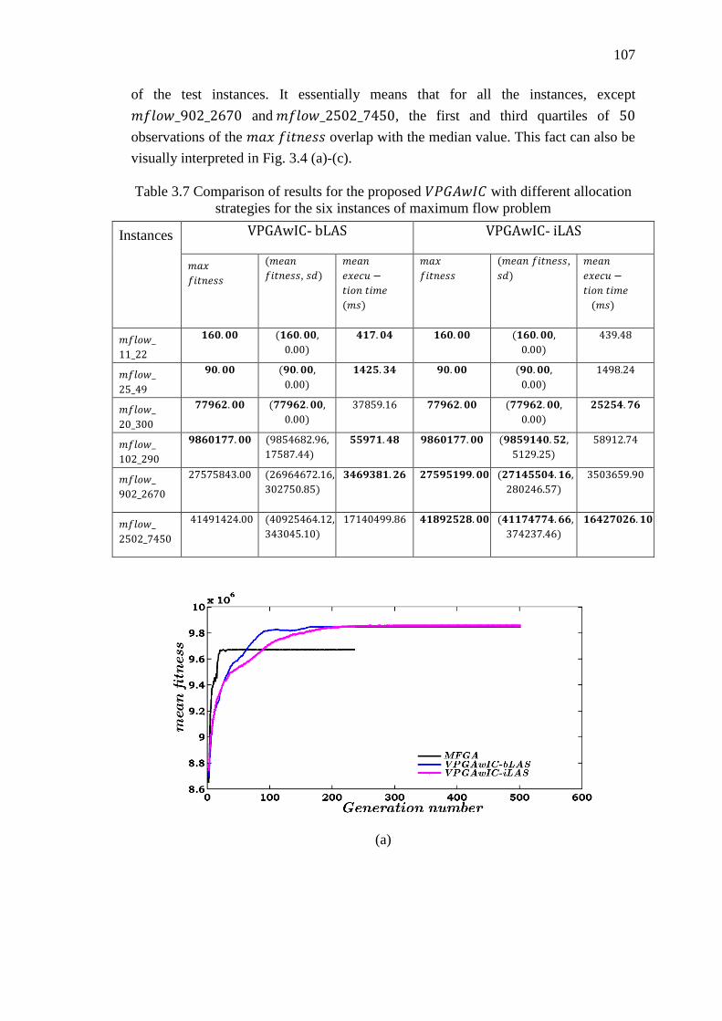
107

of the test instances. It essentially means that for all the instances, except

𝑚𝑓𝑙𝑜𝑤_902_2670 and 𝑚𝑓𝑙𝑜𝑤_2502_7450, the first and third quartiles of 50

observations of the 𝑚𝑎𝑥 𝑓𝑖𝑡𝑛𝑒𝑠𝑠 overlap with the median value. This fact can also be

visually interpreted in Fig. 3.4 (a)-(c).

Table 3.7 Comparison of results for the proposed 𝑉𝑃𝐺𝐴𝑤𝐼𝐶 with different allocation

strategies for the six instances of maximum flow problem

Instances VPGAwIC- bLAS VPGAwIC- iLAS

𝑚𝑎𝑥


(𝑚𝑒𝑎𝑛


𝑚𝑒𝑎𝑛



(𝑚𝑠)

𝑚𝑎𝑥


(𝑚𝑒𝑎𝑛 𝑓𝑖𝑡𝑛𝑒𝑠𝑠,

𝑠𝑑)

𝑚𝑒𝑎𝑛



(𝑚𝑠)


11_22

𝟏𝟔𝟎. 𝟎𝟎 (𝟏𝟔𝟎. 𝟎𝟎,

0.00)

𝟒𝟏𝟕. 𝟎𝟒 𝟏𝟔𝟎. 𝟎𝟎 (𝟏𝟔𝟎. 𝟎𝟎,

0.00)

439.48


25_49

𝟗𝟎. 𝟎𝟎 (𝟗𝟎. 𝟎𝟎,

0.00)

𝟏𝟒𝟐𝟓. 𝟑𝟒 𝟗𝟎. 𝟎𝟎 (𝟗𝟎. 𝟎𝟎,

0.00)

1498.24


20_300

𝟕𝟕𝟗𝟔𝟐. 𝟎𝟎 (𝟕𝟕𝟗𝟔𝟐. 𝟎𝟎,

0.00)

37859.16 𝟕𝟕𝟗𝟔𝟐. 𝟎𝟎 (𝟕𝟕𝟗𝟔𝟐. 𝟎𝟎,

0.00)

𝟐𝟓𝟐𝟓𝟒. 𝟕𝟔


102_290

𝟗𝟖𝟔𝟎𝟏𝟕𝟕. 𝟎𝟎 (9854682.96,

17587.44)

𝟓𝟓𝟗𝟕𝟏. 𝟒𝟖 𝟗𝟖𝟔𝟎𝟏𝟕𝟕. 𝟎𝟎 (𝟗𝟖𝟓𝟗𝟏𝟒𝟎. 𝟓𝟐,

5129.25)

58912.74


902_2670

27575843.00 (26964672.16,

302750.85)

𝟑𝟒𝟔𝟗𝟑𝟖𝟏. 𝟐𝟔 𝟐𝟕𝟓𝟗𝟓𝟏𝟗𝟗. 𝟎𝟎 (𝟐𝟕𝟏𝟒𝟓𝟓𝟎𝟒. 𝟏𝟔,

280246.57)

3503659.90


2502_7450

41491424.00 (40925464.12,

343045.10)

17140499.86 𝟒𝟏𝟖𝟗𝟐𝟓𝟐𝟖. 𝟎𝟎 (𝟒𝟏𝟏𝟕𝟒𝟕𝟕𝟒. 𝟔𝟔,

374237.46)

𝟏𝟔𝟒𝟐𝟕𝟎𝟐𝟔. 𝟏𝟎

(a)

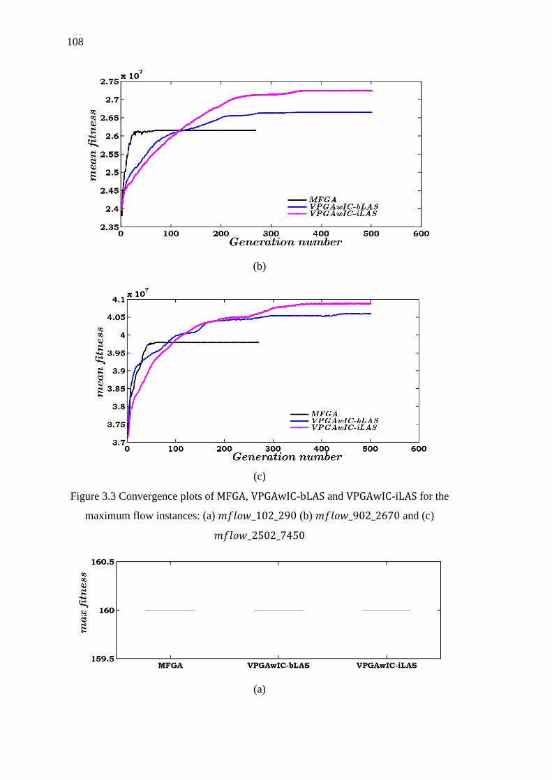
108

(b)

(c)

Figure 3.3 Convergence plots of MFGA, VPGAwIC-bLAS and VPGAwIC-iLAS for the

maximum flow instances: (a) 𝑚𝑓𝑙𝑜𝑤_102_290 (b) 𝑚𝑓𝑙𝑜𝑤_902_2670 and (c)

𝑚𝑓𝑙𝑜𝑤_2502_7450

(a)

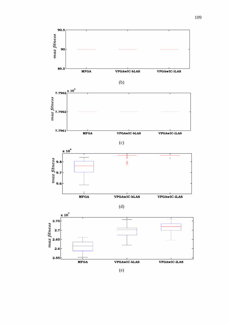
109

(b)

(c)

(d)

(e)

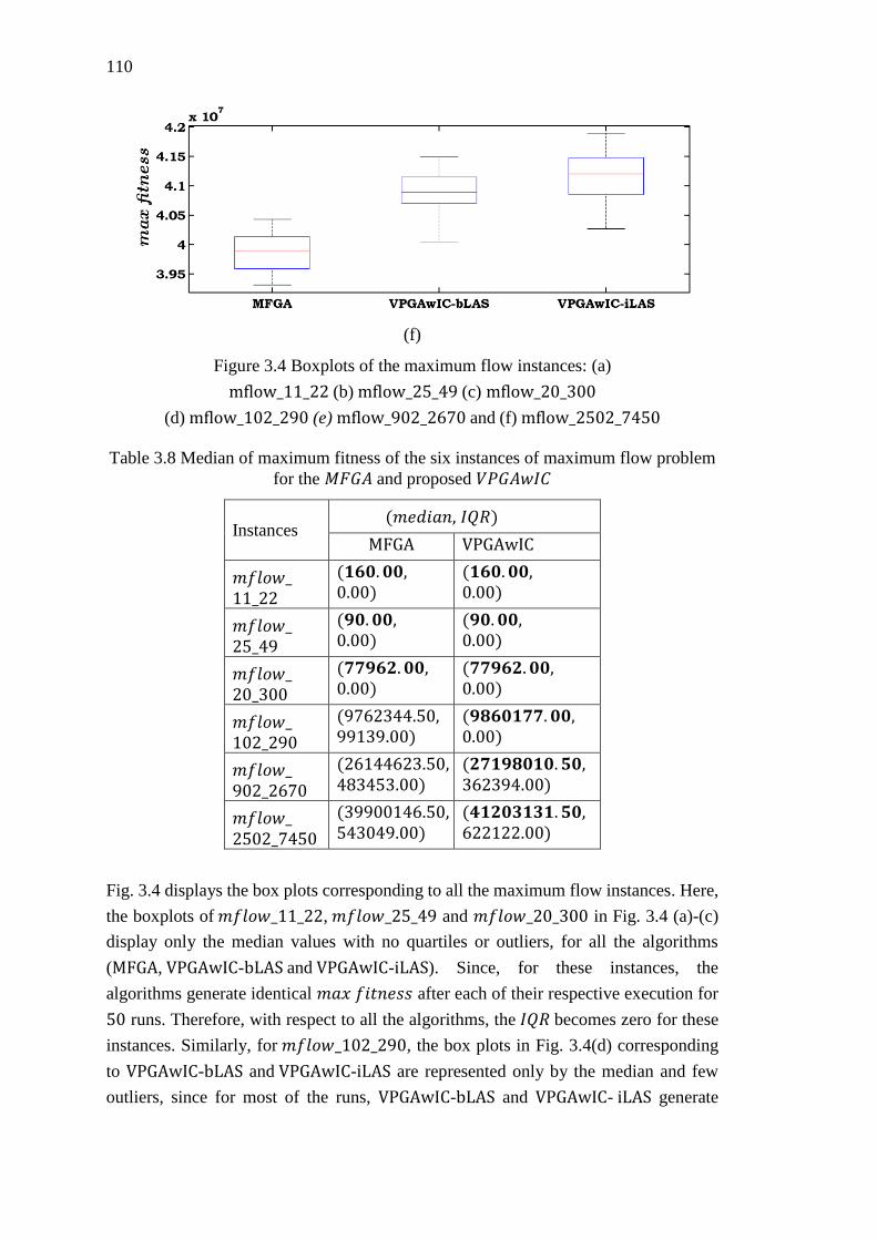
110

(f)

Figure 3.4 Boxplots of the maximum flow instances: (a)

mflow_11_22 (b) mflow_25_49 (c) mflow_20_300

(d) mflow_102_290 (e) mflow_902_2670 and (f) mflow_2502_7450


for the 𝑀𝐹𝐺𝐴 and proposed 𝑉𝑃𝐺𝐴𝑤𝐼𝐶

Fig. 3.4 displays the box plots corresponding to all the maximum flow instances. Here,

the boxplots of 𝑚𝑓𝑙𝑜𝑤_11_22, 𝑚𝑓𝑙𝑜𝑤_25_49 and 𝑚𝑓𝑙𝑜𝑤_20_300 in Fig. 3.4 (a)-(c)

display only the median values with no quartiles or outliers, for all the algorithms

(MFGA, VPGAwIC-bLAS and VPGAwIC-iLAS). Since, for these instances, the

algorithms generate identical 𝑚𝑎𝑥 𝑓𝑖𝑡𝑛𝑒𝑠𝑠 after each of their respective execution for

50 runs. Therefore, with respect to all the algorithms, the 𝐼𝑄𝑅 becomes zero for these

instances. Similarly, for 𝑚𝑓𝑙𝑜𝑤_102_290, the box plots in Fig. 3.4(d) corresponding

to VPGAwIC-bLAS and VPGAwIC-iLAS are represented only by the median and few

outliers, since for most of the runs, VPGAwIC-bLAS and VPGAwIC- iLAS generate

Instances (𝑚𝑒𝑑𝑖𝑎𝑛, 𝐼𝑄𝑅)

MFGA VPGAwIC

𝑚𝑓𝑙𝑜𝑤_ 11_22

(𝟏𝟔𝟎. 𝟎𝟎, 0.00)

(𝟏𝟔𝟎. 𝟎𝟎, 0.00)


(𝟗𝟎. 𝟎𝟎, 0.00)

(𝟗𝟎. 𝟎𝟎, 0.00)

𝑚𝑓𝑙𝑜𝑤_ 20_300

(𝟕𝟕𝟗𝟔𝟐. 𝟎𝟎, 0.00)

(𝟕𝟕𝟗𝟔𝟐. 𝟎𝟎, 0.00)

𝑚𝑓𝑙𝑜𝑤_ 102_290

(9762344.50, 99139.00)

(𝟗𝟖𝟔𝟎𝟏𝟕𝟕. 𝟎𝟎, 0.00)

𝑚𝑓𝑙𝑜𝑤_ 902_2670

(26144623.50, 483453.00)

(𝟐𝟕𝟏𝟗𝟖𝟎𝟏𝟎. 𝟓𝟎, 362394.00)

𝑚𝑓𝑙𝑜𝑤_ 2502_7450

(39900146.50, 543049.00)

(𝟒𝟏𝟐𝟎𝟑𝟏𝟑𝟏. 𝟓𝟎, 622122.00)

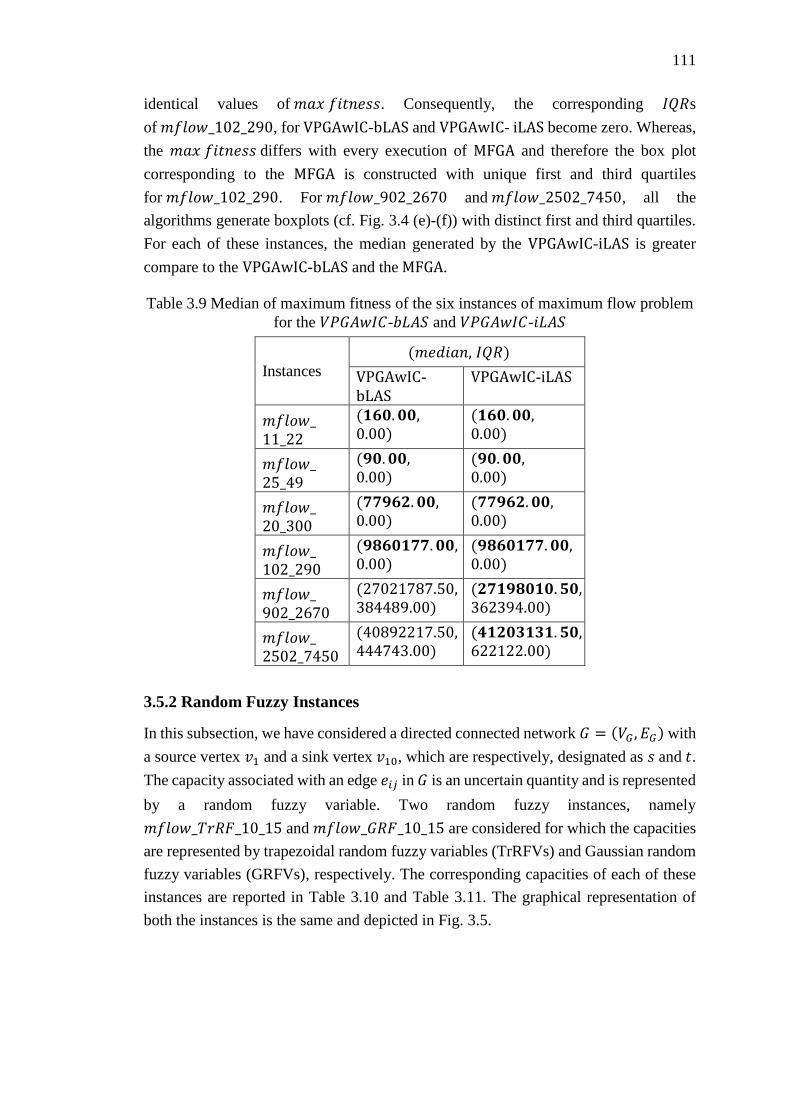
111

identical values of 𝑚𝑎𝑥 𝑓𝑖𝑡𝑛𝑒𝑠𝑠. Consequently, the corresponding 𝐼𝑄𝑅s

of 𝑚𝑓𝑙𝑜𝑤_102_290, for VPGAwIC-bLAS and VPGAwIC- iLAS become zero. Whereas,

the 𝑚𝑎𝑥 𝑓𝑖𝑡𝑛𝑒𝑠𝑠 differs with every execution of MFGA and therefore the box plot

corresponding to the MFGA is constructed with unique first and third quartiles

for 𝑚𝑓𝑙𝑜𝑤_102_290. For 𝑚𝑓𝑙𝑜𝑤_902_2670 and 𝑚𝑓𝑙𝑜𝑤_2502_7450, all the

algorithms generate boxplots (cf. Fig. 3.4 (e)-(f)) with distinct first and third quartiles.

For each of these instances, the median generated by the VPGAwIC-iLAS is greater

compare to the VPGAwIC-bLAS and the MFGA.


for the 𝑉𝑃𝐺𝐴𝑤𝐼𝐶-𝑏𝐿𝐴𝑆 and 𝑉𝑃𝐺𝐴𝑤𝐼𝐶-𝑖𝐿𝐴𝑆

3.5.2 Random Fuzzy Instances

In this subsection, we have considered a directed connected network 𝐺 = (𝑉𝐺 , 𝐸𝐺) with

a source vertex 𝑣1 and a sink vertex 𝑣10, which are respectively, designated as 𝑠 and 𝑡.

The capacity associated with an edge 𝑒𝑖𝑗 in 𝐺 is an uncertain quantity and is represented

by a random fuzzy variable. Two random fuzzy instances, namely

𝑚𝑓𝑙𝑜𝑤_𝑇𝑟𝑅𝐹_10_15 and 𝑚𝑓𝑙𝑜𝑤_𝐺𝑅𝐹_10_15 are considered for which the capacities

are represented by trapezoidal random fuzzy variables (TrRFVs) and Gaussian random

fuzzy variables (GRFVs), respectively. The corresponding capacities of each of these

instances are reported in Table 3.10 and Table 3.11. The graphical representation of

both the instances is the same and depicted in Fig. 3.5.

Instances

(𝑚𝑒𝑑𝑖𝑎𝑛, 𝐼𝑄𝑅)

VPGAwIC-

bLAS

VPGAwIC-iLAS


(𝟏𝟔𝟎. 𝟎𝟎, 0.00)

(𝟏𝟔𝟎. 𝟎𝟎, 0.00)


(𝟗𝟎. 𝟎𝟎, 0.00)

(𝟗𝟎. 𝟎𝟎, 0.00)

𝑚𝑓𝑙𝑜𝑤_ 20_300

(𝟕𝟕𝟗𝟔𝟐. 𝟎𝟎, 0.00)

(𝟕𝟕𝟗𝟔𝟐. 𝟎𝟎, 0.00)

𝑚𝑓𝑙𝑜𝑤_ 102_290

(𝟗𝟖𝟔𝟎𝟏𝟕𝟕. 𝟎𝟎, 0.00)

(𝟗𝟖𝟔𝟎𝟏𝟕𝟕. 𝟎𝟎, 0.00)

𝑚𝑓𝑙𝑜𝑤_ 902_2670

(27021787.50, 384489.00)

(𝟐𝟕𝟏𝟗𝟖𝟎𝟏𝟎. 𝟓𝟎, 362394.00)

𝑚𝑓𝑙𝑜𝑤_ 2502_7450

(40892217.50, 444743.00)

(𝟒𝟏𝟐𝟎𝟑𝟏𝟑𝟏. 𝟓𝟎, 622122.00)

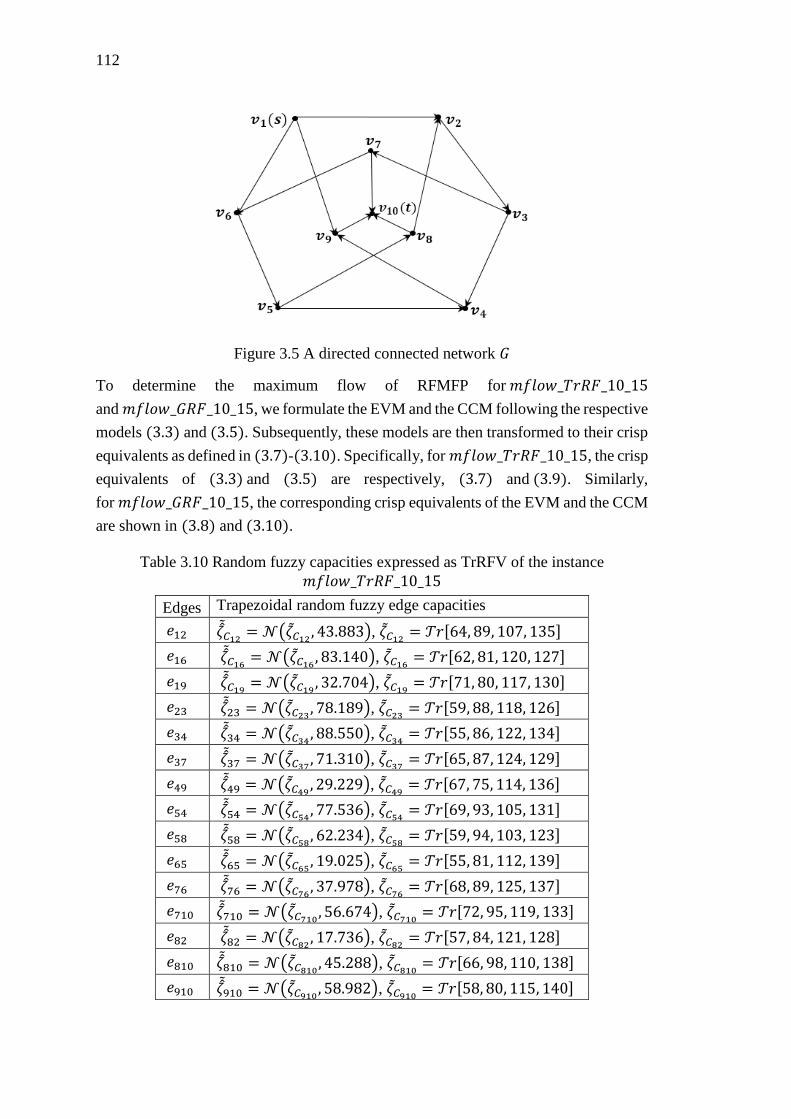
112

Figure 3.5 A directed connected network 𝐺

To determine the maximum flow of RFMFP for 𝑚𝑓𝑙𝑜𝑤_𝑇𝑟𝑅𝐹_10_15

and 𝑚𝑓𝑙𝑜𝑤_𝐺𝑅𝐹_10_15, we formulate the EVM and the CCM following the respective

models (3.3) and (3.5). Subsequently, these models are then transformed to their crisp

equivalents as defined in (3.7)-(3.10). Specifically, for 𝑚𝑓𝑙𝑜𝑤_𝑇𝑟𝑅𝐹_10_15, the crisp

equivalents of (3.3) and (3.5) are respectively, (3.7) and (3.9). Similarly,

for 𝑚𝑓𝑙𝑜𝑤_𝐺𝑅𝐹_10_15, the corresponding crisp equivalents of the EVM and the CCM

are shown in (3.8) and (3.10).

Table 3.10 Random fuzzy capacities expressed as TrRFV of the instance

𝑚𝑓𝑙𝑜𝑤_𝑇𝑟𝑅𝐹_10_15

Edges Trapezoidal random fuzzy edge capacities

𝑒12 휁𝐶12 = 𝒩(휁𝐶12 , 43.883), 휁𝐶12 = 𝒯𝑟[64, 89, 107, 135]

𝑒16 휁𝐶16 = 𝒩(휁𝐶16 , 83.140), 휁𝐶16 = 𝒯𝑟[62, 81, 120, 127]

𝑒19 휁𝐶19 = 𝒩(휁𝐶19 , 32.704), 휁𝐶19 = 𝒯𝑟[71, 80, 117, 130]

𝑒23 휁23 = 𝒩(휁𝐶23 , 78.189), 휁𝐶23 = 𝒯𝑟[59, 88, 118, 126]

𝑒34 휁34 = 𝒩(휁𝐶34 , 88.550), 휁𝐶34 = 𝒯𝑟[55, 86, 122, 134]

𝑒37 휁37 = 𝒩(휁𝐶37 , 71.310), 휁𝐶37 = 𝒯𝑟[65, 87, 124, 129]

𝑒49 휁49 = 𝒩(휁𝐶49 , 29.229), 휁𝐶49 = 𝒯𝑟[67, 75, 114, 136]

𝑒54 휁54 = 𝒩(휁𝐶54 , 77.536), 휁𝐶54 = 𝒯𝑟[69, 93, 105, 131]

𝑒58 휁58 = 𝒩(휁𝐶58 , 62.234), 휁𝐶58 = 𝒯𝑟[59, 94, 103, 123]

𝑒65 휁65 = 𝒩(휁𝐶65 , 19.025), 휁𝐶65 = 𝒯𝑟[55, 81, 112, 139]

𝑒76 휁76 = 𝒩(휁𝐶76 , 37.978), 휁𝐶76 = 𝒯𝑟[68, 89, 125, 137]

𝑒710 휁710 = 𝒩(휁𝐶710 , 56.674), 휁𝐶710 = 𝒯𝑟[72, 95, 119, 133]

𝑒82 휁82 = 𝒩(휁𝐶82 , 17.736), 휁𝐶82 = 𝒯𝑟[57, 84, 121, 128]

𝑒810 휁810 = 𝒩(휁𝐶810 , 45.288), 휁𝐶810 = 𝒯𝑟[66, 98, 110, 138]

𝑒910 휁910 = 𝒩(휁𝐶910 , 58.982), 휁𝐶910 = 𝒯𝑟[58, 80, 115, 140]

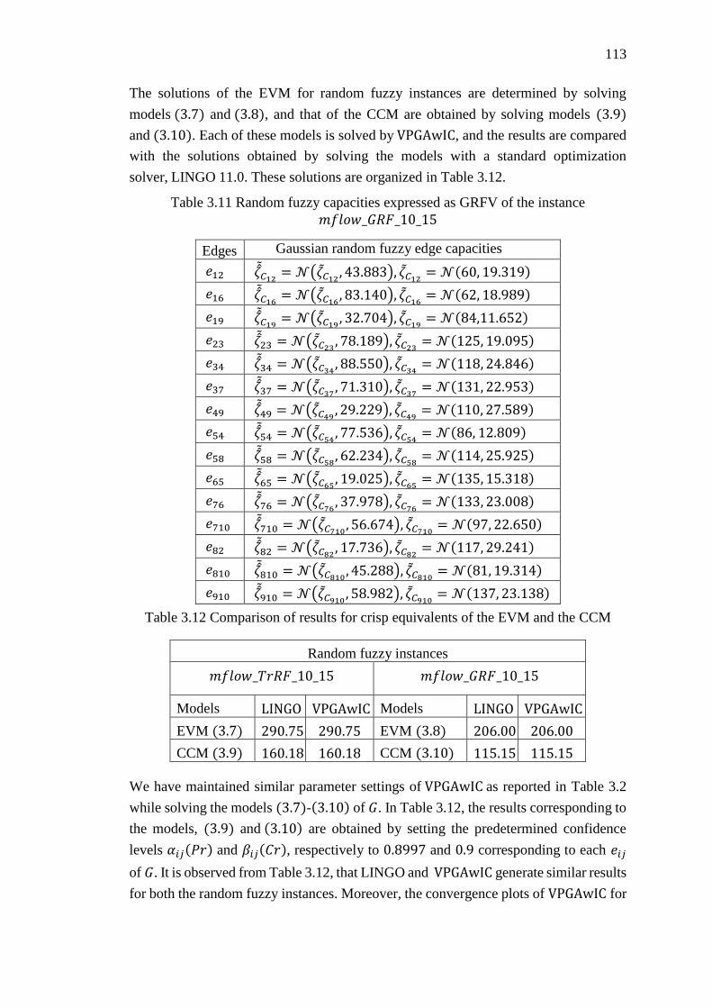
113

The solutions of the EVM for random fuzzy instances are determined by solving

models (3.7) and (3.8), and that of the CCM are obtained by solving models (3.9)

and (3.10). Each of these models is solved by VPGAwIC, and the results are compared

with the solutions obtained by solving the models with a standard optimization

solver, LINGO 11.0. These solutions are organized in Table 3.12.

Table 3.11 Random fuzzy capacities expressed as GRFV of the instance

𝑚𝑓𝑙𝑜𝑤_𝐺𝑅𝐹_10_15

Edges Gaussian random fuzzy edge capacities

𝑒12 휁𝐶12 = 𝒩(휁𝐶12 , 43.883), 휁𝐶12 = 𝒩(60, 19.319)

𝑒16 휁𝐶16 = 𝒩(휁𝐶16 , 83.140), 휁𝐶16 = 𝒩(62, 18.989)

𝑒19 휁𝐶19 = 𝒩(휁𝐶19 , 32.704), 휁𝐶19 = 𝒩(84,11.652)

𝑒23 휁23 = 𝒩(휁𝐶23 , 78.189), 휁𝐶23 = 𝒩(125, 19.095)

𝑒34 휁34 = 𝒩(휁𝐶34 , 88.550), 휁𝐶34 = 𝒩(118, 24.846)

𝑒37 휁37 = 𝒩(휁𝐶37 , 71.310), 휁𝐶37 = 𝒩(131, 22.953)

𝑒49 휁49 = 𝒩(휁𝐶49 , 29.229), 휁𝐶49 = 𝒩(110, 27.589)

𝑒54 휁54 = 𝒩(휁𝐶54 , 77.536), 휁𝐶54 = 𝒩(86, 12.809)

𝑒58 휁58 = 𝒩(휁𝐶58 , 62.234), 휁𝐶58 = 𝒩(114, 25.925)

𝑒65 휁65 = 𝒩(휁𝐶65 , 19.025), 휁𝐶65 = 𝒩(135, 15.318)

𝑒76 휁76 = 𝒩(휁𝐶76 , 37.978), 휁𝐶76 = 𝒩(133, 23.008)

𝑒710 휁710 = 𝒩(휁𝐶710 , 56.674), 휁𝐶710 = 𝒩(97, 22.650)

𝑒82 휁82 = 𝒩(휁𝐶82 , 17.736), 휁𝐶82 = 𝒩(117, 29.241)

𝑒810 휁810 = 𝒩(휁𝐶810 , 45.288), 휁𝐶810 = 𝒩(81, 19.314)

𝑒910 휁910 = 𝒩(휁𝐶910 , 58.982), 휁𝐶910 = 𝒩(137, 23.138)

Table 3.12 Comparison of results for crisp equivalents of the EVM and the CCM

We have maintained similar parameter settings of VPGAwIC as reported in Table 3.2

while solving the models (3.7)-(3.10) of 𝐺. In Table 3.12, the results corresponding to

the models, (3.9) and (3.10) are obtained by setting the predetermined confidence

levels 𝛼𝑖𝑗(𝑃𝑟) and 𝛽𝑖𝑗(𝐶𝑟), respectively to 0.8997 and 0.9 corresponding to each 𝑒𝑖𝑗

of 𝐺. It is observed from Table 3.12, that LINGO and VPGAwIC generate similar results

for both the random fuzzy instances. Moreover, the convergence plots of VPGAwIC for

Random fuzzy instances

𝑚𝑓𝑙𝑜𝑤_𝑇𝑟𝑅𝐹_10_15 𝑚𝑓𝑙𝑜𝑤_𝐺𝑅𝐹_10_15

Models LINGO VPGAwIC Models LINGO VPGAwIC

EVM (3.7) 290.75 290.75 EVM (3.8) 206.00 206.00

CCM (3.9) 160.18 160.18 CCM (3.10) 115.15 115.15

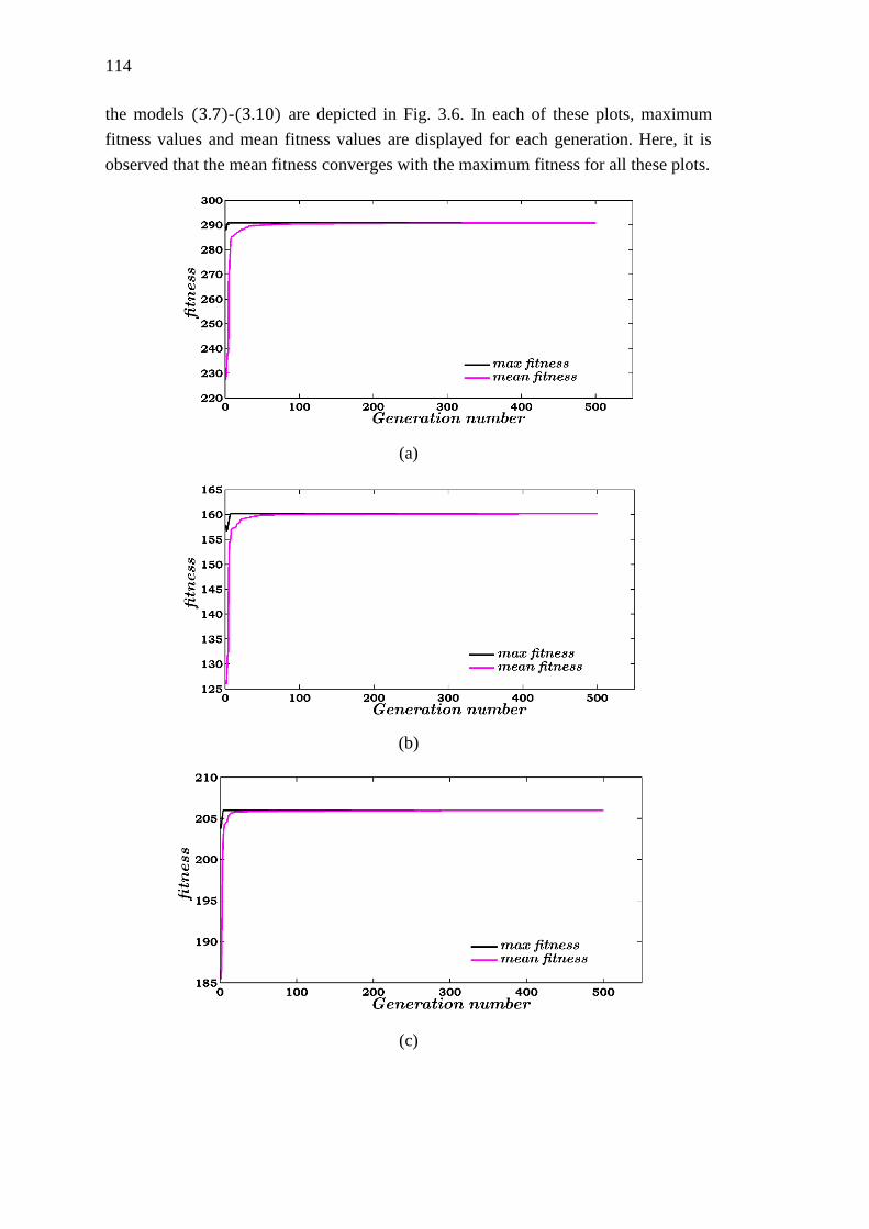
114

the models (3.7)-(3.10) are depicted in Fig. 3.6. In each of these plots, maximum

fitness values and mean fitness values are displayed for each generation. Here, it is

observed that the mean fitness converges with the maximum fitness for all these plots.

(a)

(b)

(c)

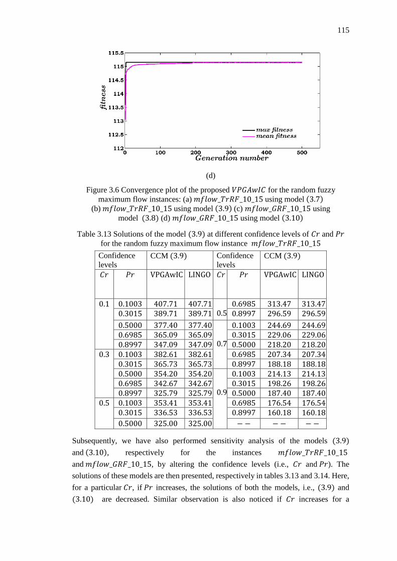
115

(d)

Figure 3.6 Convergence plot of the proposed 𝑉𝑃𝐺𝐴𝑤𝐼𝐶 for the random fuzzy

maximum flow instances: (a) 𝑚𝑓𝑙𝑜𝑤_𝑇𝑟𝑅𝐹_10_15 using model (3.7) (b) 𝑚𝑓𝑙𝑜𝑤_𝑇𝑟𝑅𝐹_10_15 using model (3.9) (c) 𝑚𝑓𝑙𝑜𝑤_𝐺𝑅𝐹_10_15 using

model (3.8) (d) 𝑚𝑓𝑙𝑜𝑤_𝐺𝑅𝐹_10_15 using model (3.10)


for the random fuzzy maximum flow instance 𝑚𝑓𝑙𝑜𝑤_𝑇𝑟𝑅𝐹_10_15

Confidence

levels CCM (3.9) Confidence

levels CCM (3.9)

𝐶𝑟 𝑃𝑟 VPGAwIC

LINGO


LINGO

0.1 0.1003 407.71 407.71

0.5

0.6985 313.47 313.47

0.3015 389.71 389.71 0.8997 296.59 296.59

0.5000 377.40 377.40

0.7

0.1003 244.69 244.69 0.6985 365.09 365.09 0.3015 229.06 229.06 0.8997 347.09 347.09 0.5000 218.20 218.20

0.3 0.1003 382.61 382.61 0.6985 207.34 207.34 0.3015 365.73 365.73 0.8997 188.18 188.18 0.5000 354.20 354.20

0.9

0.1003 214.13 214.13 0.6985 342.67 342.67 0.3015 198.26 198.26 0.8997 325.79 325.79 0.5000 187.40 187.40

0.5 0.1003 353.41 353.41 0.6985 176.54 176.54 0.3015 336.53 336.53 0.8997 160.18 160.18

0.5000 325.00 325.00 −− −− − −

Subsequently, we have also performed sensitivity analysis of the models (3.9)

and (3.10), respectively for the instances 𝑚𝑓𝑙𝑜𝑤_𝑇𝑟𝑅𝐹_10_15

and 𝑚𝑓𝑙𝑜𝑤_𝐺𝑅𝐹_10_15, by altering the confidence levels (i.e., 𝐶𝑟 and 𝑃𝑟). The

solutions of these models are then presented, respectively in tables 3.13 and 3.14. Here,

for a particular 𝐶𝑟, if 𝑃𝑟 increases, the solutions of both the models, i.e., (3.9) and

(3.10) are decreased. Similar observation is also noticed if 𝐶𝑟 increases for a

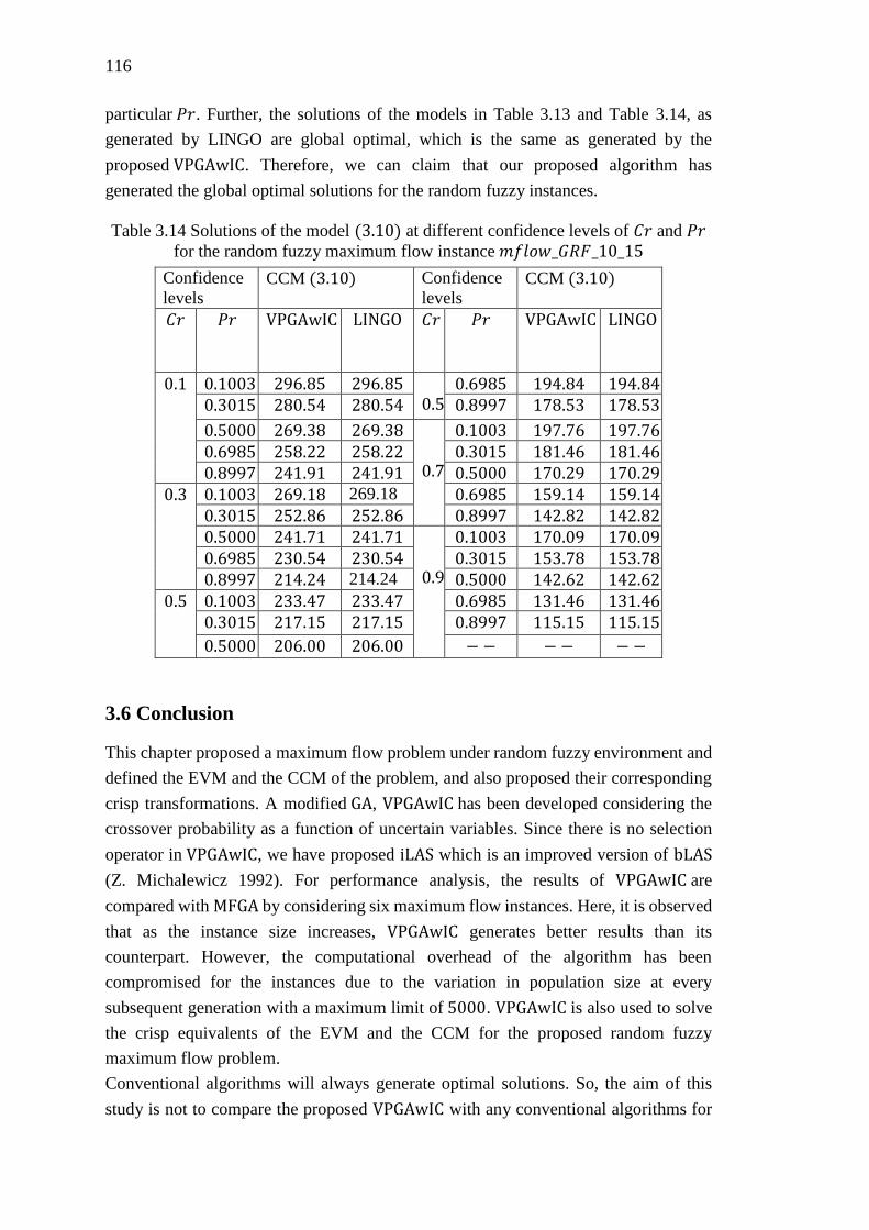
116

particular 𝑃𝑟. Further, the solutions of the models in Table 3.13 and Table 3.14, as

generated by LINGO are global optimal, which is the same as generated by the

proposed VPGAwIC. Therefore, we can claim that our proposed algorithm has

generated the global optimal solutions for the random fuzzy instances.


for the random fuzzy maximum flow instance 𝑚𝑓𝑙𝑜𝑤_𝐺𝑅𝐹_10_15

Confidence

levels CCM (3.10) Confidence

levels CCM (3.10)


LINGO


LINGO

0.1 0.1003 296.85 296.85

0.5

0.6985 194.84 194.84

0.3015 280.54 280.54 0.8997 178.53 178.53

0.5000 269.38 269.38

0.7

0.1003 197.76 197.76 0.6985 258.22 258.22 0.3015 181.46 181.46 0.8997 241.91 241.91 0.5000 170.29 170.29

0.3 0.1003 269.18 269.18 0.6985 159.14 159.14 0.3015 252.86 252.86 0.8997 142.82 142.82 0.5000 241.71 241.71

0.9

0.1003 170.09 170.09 0.6985 230.54 230.54 0.3015 153.78 153.78 0.8997 214.24 214.24 0.5000 142.62 142.62

0.5 0.1003 233.47 233.47 0.6985 131.46 131.46 0.3015 217.15 217.15 0.8997 115.15 115.15

0.5000 206.00 206.00 − − −− −−

3.6 Conclusion

This chapter proposed a maximum flow problem under random fuzzy environment and

defined the EVM and the CCM of the problem, and also proposed their corresponding

crisp transformations. A modified GA, VPGAwIC has been developed considering the

crossover probability as a function of uncertain variables. Since there is no selection

operator in VPGAwIC, we have proposed iLAS which is an improved version of bLAS

(Z. Michalewicz 1992). For performance analysis, the results of VPGAwIC are

compared with MFGA by considering six maximum flow instances. Here, it is observed

that as the instance size increases, VPGAwIC generates better results than its

counterpart. However, the computational overhead of the algorithm has been

compromised for the instances due to the variation in population size at every

subsequent generation with a maximum limit of 5000. VPGAwIC is also used to solve

the crisp equivalents of the EVM and the CCM for the proposed random fuzzy


Conventional algorithms will always generate optimal solutions. So, the aim of this

study is not to compare the proposed VPGAwIC with any conventional algorithms for

117

maximum flow problem. However, many real-life problems can be modelled as

different variants of the maximum flow problem (e.g., maximum flow problem with

minimum quantities (Haugland et al. 2011, Thielen and Westphal 2013), maximum

flow-minimum cost bi-objective problem, etc.), where the complexity of the problem

potentially increases due to additional constraints and/or objectives. In those cases,

genetic algorithms can be designed/redesigned to generate near-optimal solutions of

those problems including their larger instances. However, in this context, conventional

algorithms may not be able to generate the solutions.

In future, this study will provide a base while determining efficient solution procedure

for maximum-flow based combinatorial optimization problems under uncertain

environment. The maximum flow problem can also be extended to maximum flow

minimum cost bi-objective problem under uncertain environment, which can be solved

by considering a multi-objective version of VPGAwIC in future.

118

User

Text Box

114

Part-II

Uncertain Multi-Objective Optimization

Problems

Chapter 4

Chapter 5

Chapter 6

USER

Text Box

120

User

Text Box

121

Chapter 4

Multi-criteria Shortest Path Problem on

Rough Graph

User

Text Box

122

User

Text Box

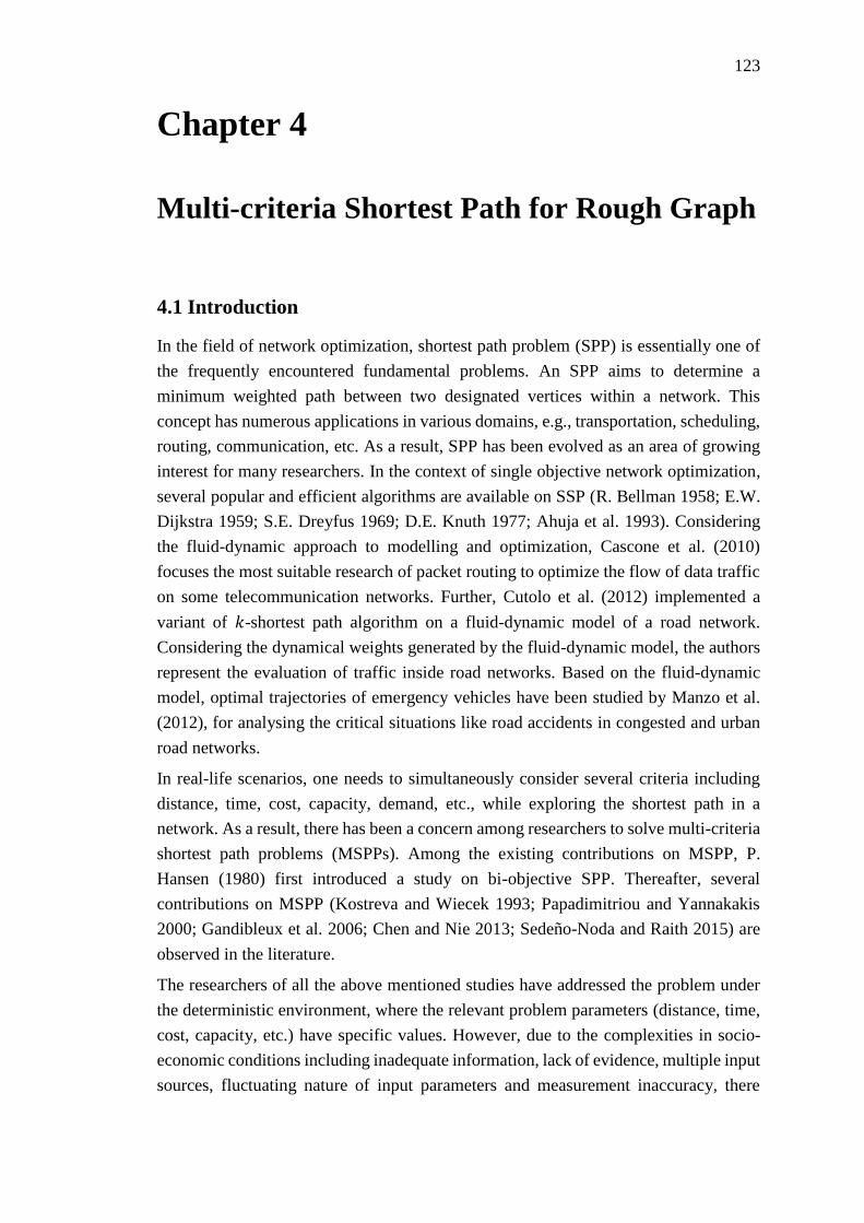
123

Chapter 4

Multi-criteria Shortest Path for Rough Graph

4.1 Introduction

In the field of network optimization, shortest path problem (SPP) is essentially one of

the frequently encountered fundamental problems. An SPP aims to determine a

minimum weighted path between two designated vertices within a network. This

concept has numerous applications in various domains, e.g., transportation, scheduling,

routing, communication, etc. As a result, SPP has been evolved as an area of growing

interest for many researchers. In the context of single objective network optimization,

several popular and efficient algorithms are available on SSP (R. Bellman 1958; E.W.

Dijkstra 1959; S.E. Dreyfus 1969; D.E. Knuth 1977; Ahuja et al. 1993). Considering

the fluid-dynamic approach to modelling and optimization, Cascone et al. (2010)

focuses the most suitable research of packet routing to optimize the flow of data traffic

on some telecommunication networks. Further, Cutolo et al. (2012) implemented a

variant of 𝑘-shortest path algorithm on a fluid-dynamic model of a road network.

Considering the dynamical weights generated by the fluid-dynamic model, the authors

represent the evaluation of traffic inside road networks. Based on the fluid-dynamic

model, optimal trajectories of emergency vehicles have been studied by Manzo et al.

(2012), for analysing the critical situations like road accidents in congested and urban

road networks.

In real-life scenarios, one needs to simultaneously consider several criteria including

distance, time, cost, capacity, demand, etc., while exploring the shortest path in a

network. As a result, there has been a concern among researchers to solve multi-criteria

shortest path problems (MSPPs). Among the existing contributions on MSPP, P.

Hansen (1980) first introduced a study on bi-objective SPP. Thereafter, several

contributions on MSPP (Kostreva and Wiecek 1993; Papadimitriou and Yannakakis

2000; Gandibleux et al. 2006; Chen and Nie 2013; Sedeño-Noda and Raith 2015) are

observed in the literature.

The researchers of all the above mentioned studies have addressed the problem under

the deterministic environment, where the relevant problem parameters (distance, time,

cost, capacity, etc.) have specific values. However, due to the complexities in socio-

economic conditions including inadequate information, lack of evidence, multiple input

sources, fluctuating nature of input parameters and measurement inaccuracy, there

User

Text Box

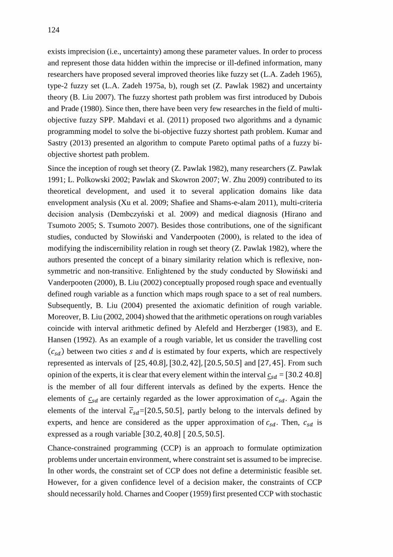
124

exists imprecision (i.e., uncertainty) among these parameter values. In order to process

and represent those data hidden within the imprecise or ill-defined information, many

researchers have proposed several improved theories like fuzzy set (L.A. Zadeh 1965),

type-2 fuzzy set (L.A. Zadeh 1975a, b), rough set (Z. Pawlak 1982) and uncertainty

theory (B. Liu 2007). The fuzzy shortest path problem was first introduced by Dubois

and Prade (1980). Since then, there have been very few researches in the field of multi-

objective fuzzy SPP. Mahdavi et al. (2011) proposed two algorithms and a dynamic

programming model to solve the bi-objective fuzzy shortest path problem. Kumar and

Sastry (2013) presented an algorithm to compute Pareto optimal paths of a fuzzy bi-

objective shortest path problem.

Since the inception of rough set theory (Z. Pawlak 1982), many researchers (Z. Pawlak

1991; L. Polkowski 2002; Pawlak and Skowron 2007; W. Zhu 2009) contributed to its

theoretical development, and used it to several application domains like data

envelopment analysis (Xu et al. 2009; Shafiee and Shams-e-alam 2011), multi-criteria

decision analysis (Dembczyński et al. 2009) and medical diagnosis (Hirano and

Tsumoto 2005; S. Tsumoto 2007). Besides those contributions, one of the significant

studies, conducted by Słowiński and Vanderpooten (2000), is related to the idea of

modifying the indiscernibility relation in rough set theory (Z. Pawlak 1982), where the

authors presented the concept of a binary similarity relation which is reflexive, non-

symmetric and non-transitive. Enlightened by the study conducted by Słowiński and

Vanderpooten (2000), B. Liu (2002) conceptually proposed rough space and eventually

defined rough variable as a function which maps rough space to a set of real numbers.

Subsequently, B. Liu (2004) presented the axiomatic definition of rough variable.

Moreover, B. Liu (2002, 2004) showed that the arithmetic operations on rough variables

coincide with interval arithmetic defined by Alefeld and Herzberger (1983), and E.

Hansen (1992). As an example of a rough variable, let us consider the travelling cost

(𝑐𝑠𝑑) between two cities 𝑠 and 𝑑 is estimated by four experts, which are respectively

represented as intervals of [25, 40.8], [30.2, 42], [20.5, 50.5] and [27, 45]. From such

opinion of the experts, it is clear that every element within the interval 𝑐𝑠𝑑 = [30.2 40.8]

is the member of all four different intervals as defined by the experts. Hence the

elements of 𝑐𝑠𝑑 are certainly regarded as the lower approximation of 𝑐𝑠𝑑. Again the

elements of the interval 𝑐𝑠𝑑=[20.5, 50.5], partly belong to the intervals defined by

experts, and hence are considered as the upper approximation of 𝑐𝑠𝑑. Then, 𝑐𝑠𝑑 is

expressed as a rough variable [30.2, 40.8] [ 20.5, 50.5].

Chance-constrained programming (CCP) is an approach to formulate optimization

problems under uncertain environment, where constraint set is assumed to be imprecise.

In other words, the constraint set of CCP does not define a deterministic feasible set.

However, for a given confidence level of a decision maker, the constraints of CCP

should necessarily hold. Charnes and Cooper (1959) first presented CCP with stochastic

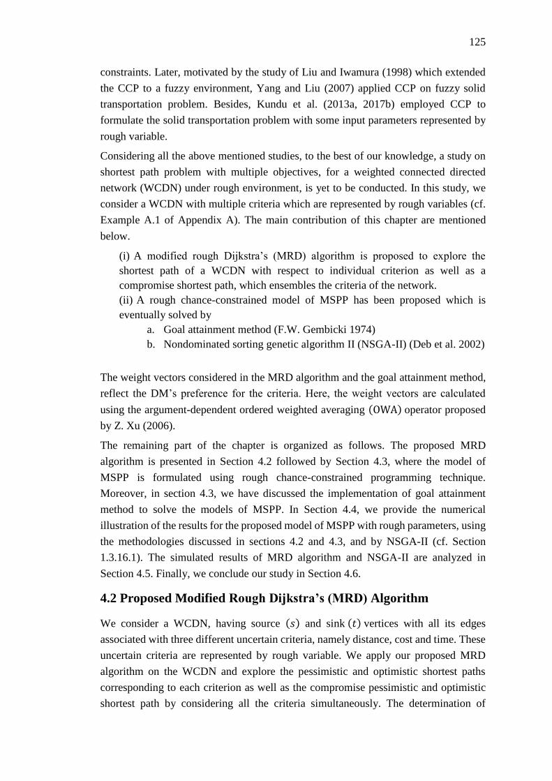
125

constraints. Later, motivated by the study of Liu and Iwamura (1998) which extended

the CCP to a fuzzy environment, Yang and Liu (2007) applied CCP on fuzzy solid

transportation problem. Besides, Kundu et al. (2013a, 2017b) employed CCP to

formulate the solid transportation problem with some input parameters represented by

rough variable.

Considering all the above mentioned studies, to the best of our knowledge, a study on

shortest path problem with multiple objectives, for a weighted connected directed

network (WCDN) under rough environment, is yet to be conducted. In this study, we

consider a WCDN with multiple criteria which are represented by rough variables (cf.

Example A.1 of Appendix A). The main contribution of this chapter are mentioned

below.

(i) A modified rough Dijkstra’s (MRD) algorithm is proposed to explore the

shortest path of a WCDN with respect to individual criterion as well as a

compromise shortest path, which ensembles the criteria of the network.

(ii) A rough chance-constrained model of MSPP has been proposed which is

eventually solved by

a. Goal attainment method (F.W. Gembicki 1974)

b. Nondominated sorting genetic algorithm II (NSGA-II) (Deb et al. 2002)

The weight vectors considered in the MRD algorithm and the goal attainment method,

reflect the DM’s preference for the criteria. Here, the weight vectors are calculated

using the argument-dependent ordered weighted averaging (OWA) operator proposed

by Z. Xu (2006).

The remaining part of the chapter is organized as follows. The proposed MRD

algorithm is presented in Section 4.2 followed by Section 4.3, where the model of

MSPP is formulated using rough chance-constrained programming technique.

Moreover, in section 4.3, we have discussed the implementation of goal attainment

method to solve the models of MSPP. In Section 4.4, we provide the numerical

illustration of the results for the proposed model of MSPP with rough parameters, using

the methodologies discussed in sections 4.2 and 4.3, and by NSGA-II (cf. Section

1.3.16.1). The simulated results of MRD algorithm and NSGA-II are analyzed in

Section 4.5. Finally, we conclude our study in Section 4.6.

4.2 Proposed Modified Rough Dijkstra’s (MRD) Algorithm

We consider a WCDN, having source (𝑠) and sink (𝑡) vertices with all its edges

associated with three different uncertain criteria, namely distance, cost and time. These

uncertain criteria are represented by rough variable. We apply our proposed MRD

algorithm on the WCDN and explore the pessimistic and optimistic shortest paths

corresponding to each criterion as well as the compromise pessimistic and optimistic

shortest path by considering all the criteria simultaneously. The determination of

126

shortest paths is done at two different trust labels 𝑇𝑚1 and 𝑇𝑚2 such that, 0 < 𝑇𝑚1 ≤

0.5 and 0.5 < 𝑇𝑚2 ≤ 1.0. This is due to the fact that, for any rough variable, its

pessimistic value is less or equal to its optimistic value if the trust label is set

within (0,0.5]. Further, if the trust label is within (0.5,1.0], then for a rough variable,

its pessimistic value is greater or equal to its optimistic value. Here, for every edge of

a WCDN, we determine the argument-dependent OWA weights (Z. Xu 2006) with

respect to three uncertain criteria to explore the compromise pessimistic and optimistic

shortest paths.

Let 𝐺(𝑉𝐺 , 𝐸𝐺) be a WCDN, where 𝑉𝐺 and 𝐸𝐺 are the set of vertices and edges of 𝐺. The

weights of each edge 𝑒 (𝑒 ∈ 𝐸𝐺) connecting vertices 𝑣 and 𝑣′ are associated with three

uncertain criteria: distance (𝑃1), cost (𝑃2) and time (𝑃3) which are expressed as rough

variables, where 𝑃𝑘 = ([𝑃2𝑘 , 𝑃3

𝑘], [𝑃1𝑘 , 𝑃4

𝑘]), 𝑃1𝑘 ≤ 𝑃2

𝑘 < 𝑃3𝑘 ≤ 𝑃4

𝑘 ∀𝑘 ∈ {1,2,3}. For

an edge 𝑒, each 𝑃𝑗𝑘 determines an extreme bound of an approximation set of the

representing rough variable of 𝑘𝑡ℎ criterion. Since the associated weights of 𝐺 are

represented by rough variable, these weights are also termed as rough weights. Here,

if 𝑗 = 2,3 ∀𝑘 ∈ {1,2,3}, then 𝑃𝑗𝑘 determines an extreme bound of the lower

approximation set of 𝑃𝑘. Again, if 𝑗 = 1,4 ∀𝑘 ∈ {1,2,3}, then 𝑃𝑗𝑘 determines an

extreme bound of the upper approximation set of 𝑃𝑘. The steps of the MRD algorithm

are outlined below.

Input: A WCDN, 𝐺 with all the edges associated with three criteria, 𝑃1, 𝑃2 and 𝑃3

which are represented by rough variables.

Output:

(i) Pessimistic and optimistic shortest paths and their corresponding path weights

from source (𝑠) to sink (𝑡) vertices with respect to each 𝑃𝑘

(ii) Compromise pessimistic and optimistic shortest paths with their effective

weights.

at trust measures, 𝑇𝑚1and 𝑇𝑚2.

Step 1: Set the values of the trust measure 𝑇𝑚1(∈ (0,0.5]) and 𝑇𝑚2(∈ (0.5,1.0]) for

the rough weights associated with 𝐺.

Step 2: Set the label 𝐿𝑏(𝑠) of the source vertex 𝑠 such that

𝐿𝑏(𝑠)=[(0𝑝𝑒𝑠𝑠𝑖𝑃1 , 𝑠, 0𝑝𝑒𝑠𝑠𝑖

𝑃2 , 𝑠, 0𝑝𝑒𝑠𝑠𝑖𝑃3 , 𝑠, 0𝑝𝑒𝑠𝑠𝑖

𝐶𝑜𝑚𝑝, 𝑠)

𝑇𝑚𝑙,

(0𝑜𝑝𝑡𝑖𝑃1 , 𝑠, 0𝑜𝑝𝑡𝑖

𝑃2 , 𝑠, 0𝑜𝑝𝑡𝑖𝑃3 , 𝑠, 0𝑜𝑝𝑡𝑖

𝐶𝑜𝑚𝑝, 𝑠)

𝑇𝑚𝑙],

where 0𝑝𝑒𝑠𝑠𝑖𝑃𝑘 and 0𝑜𝑝𝑡𝑖

𝑃𝑘 determine the pessimistic and optimistic values of criterion 𝑃𝑘

for a trust measure, 𝑇𝑚𝑙 ∈ {𝑇𝑚1, 𝑇𝑚2} ∀𝑘 ∈ {1,2,3}. Since 𝑠 is the source vertex, then

𝑠 itself becomes its predecessor vertex, and the pessimistic and optimistic shortest paths

127

from the current vertex to its predecessor vertex, i.e., 𝑠, is set to 0𝑝𝑒𝑠𝑠𝑖𝑃𝑘 and 0𝑜𝑝𝑡𝑖

𝑃𝑘 ,

respectively ∀𝑘 ∈ {1,2,3}.

Set the labels of the remaining vertices of 𝐺 as

𝐿𝑏(𝑣𝒊)=[(∞𝑝𝑒𝑠𝑠𝑖

𝑃1 , ___, ∞𝑝𝑒𝑠𝑠𝑖𝑃2 , ___, ∞𝑝𝑒𝑠𝑠𝑖

𝑃3 , ___, ∞𝑝𝑒𝑠𝑠𝑖𝐶𝑜𝑚𝑝

, ___)𝑇𝑚𝑙

,

(∞𝑜𝑝𝑡𝑖𝑃1 , ___, ∞𝑜𝑝𝑡𝑖

𝑃2 , ___, ∞𝑜𝑝𝑡𝑖𝑃3 , ___, ∞

𝑜𝑝𝑡𝑖𝐶𝑜𝑚𝑝

, ___)𝑇𝑚𝑙

], ∀𝑣𝑖 ∈ 𝑉𝐺\{𝑠} and 𝑇𝑚𝑙 ∈

{𝑇𝑚1, 𝑇𝑚2}.

Initially, since the predecessor vertices of all 𝑣𝒊′s are unknown, therefore

The shortest distance from each 𝑣𝒊 to its immediate predecessor vertex is set as

∞𝑝𝑒𝑠𝑠𝑖𝑃𝑘 and ∞𝑜𝑝𝑡𝑖

𝑃𝑘 for pessimistic and optimistic shortest paths, respectively ∀𝑘 ∈

{1,2,3}.

The symbol ‘___’ in 𝐿𝑏(𝑣𝑖) is used to designate the unknown predecessor vertex

of 𝑣𝒊.

Step 3: For a vertex 𝑣 , find its successor vertex set 𝑆𝑟(𝑣) and the set of

edges 𝐸𝑣 𝑣′, ∀𝑣′ ∈ 𝑆𝑟(𝑣), where 𝑆𝑟(𝑣) ⊆ 𝑉𝐺 and 𝐸𝑣 𝑣′ ⊆ 𝐸𝐺 .

Step 4: For a trust label 𝑇𝑚𝑙(∈ {𝑇𝑚1, 𝑇𝑚2}), consider each edge 𝑒 ∈ 𝐸𝑣 𝑣′ to calculate

the 𝑇𝑚𝑙-pessimistic ({𝑒𝑝𝑒𝑠𝑠𝑖𝑃1 , 𝑒𝑝𝑒𝑠𝑠𝑖

𝑃2 , 𝑒𝑝𝑒𝑠𝑠𝑖𝑃3 }) and 𝑇𝑚𝑙-optimistic ({𝑒𝑜𝑝𝑡𝑖

𝑃1 , 𝑒𝑜𝑝𝑡𝑖𝑃2 , 𝑒𝑜𝑝𝑡𝑖

𝑃3 })

values corresponding to its associated edge weight 𝑒𝑃𝑘(𝑘 = {1,2,3}) using Step 4.1 and

Step 4.2, respectively.

Step 4.1:

𝑒𝑖𝑛𝑓(𝑇𝑚𝑙)=

{

(1 − 2𝑇𝑚𝑙)𝑒

𝑃1𝑘+ 2𝑇𝑚𝑙𝑒

𝑃4𝑘 ; 𝑖𝑓 𝑇𝑚𝑙 ≤ (

(𝑒𝑃2𝑘−𝑒𝑃1

𝑘)

2(𝑒𝑃4𝑘−𝑒𝑃1

𝑘))

2(1 − 𝑇𝑚𝑙)𝑒𝑃1𝑘+ (2𝑇𝑚𝑙 − 1)𝑒

𝑃4𝑘 ; 𝑖𝑓 𝑇𝑚𝑙 ≥ (

(𝑒𝑃3𝑘+𝑒𝑃4

𝑘−2𝑒𝑃1

𝑘)


𝑘))

(𝑒𝑃1

𝑘(𝑒𝑃3

𝑘−𝑒𝑃2

𝑘)+𝑒𝑃2

𝑘(𝑒𝑃4

𝑘−𝑒𝑃1

𝑘)+2𝑇𝑚𝑙(𝑒

𝑃3𝑘−𝑒𝑃2

𝑘)(𝑒𝑃4

𝑘−𝑒𝑃1

𝑘)


𝑘)+(𝑒𝑃4

𝑘−𝑒𝑃1

𝑘)

) ; 𝑜𝑡ℎ𝑒𝑟𝑤𝑖𝑠𝑒

Step 4.2:

𝑒𝑠𝑢𝑝(𝑇𝑚𝑙)=

{

(1 − 2𝑇𝑚𝑙)𝑒

𝑃4𝑘+ 2𝑇𝑚𝑙𝑒

𝑃1𝑘 ; 𝑖𝑓 𝑇𝑚𝑙 ≤ (


𝑘)


𝑘))

2(1 − 𝑇𝑚𝑙)𝑒𝑃4𝑘+ (2𝑇𝑚𝑙 − 1)𝑒

𝑃1𝑘 ; 𝑖𝑓 𝑇𝑚𝑙 ≥ (

(2𝑒𝑃4𝑘−𝑒𝑃2

𝑘−𝑒𝑃1

𝑘)


𝑘))

(𝑒𝑃4

𝑘(𝑒𝑃3

𝑘−𝑒𝑃2

𝑘)+𝑒𝑃3

𝑘(𝑒𝑃4

𝑘−𝑒𝑃1

𝑘)−2𝑇𝑚𝑙(𝑒

𝑃3𝑘−𝑒𝑃2

𝑘)(𝑒𝑃4

𝑘−𝑒𝑃1

𝑘)


𝑘)+(𝑒𝑃4

𝑘−𝑒𝑃1

𝑘)

) ; 𝑜𝑡ℎ𝑒𝑟𝑤𝑖𝑠𝑒

128

∀𝑘 ∈ {1,2,3} such that, 𝑒𝑖𝑛𝑓(𝑇𝑚𝑙) ∈ {𝑒𝑝𝑒𝑠𝑠𝑖𝑃1 , 𝑒𝑝𝑒𝑠𝑠𝑖

𝑃2 , 𝑒𝑝𝑒𝑠𝑠𝑖𝑃3 } and 𝑒𝑠𝑢𝑝(𝑇𝑚𝑙) ∈

{𝑒𝑜𝑝𝑡𝑖𝑃1 , 𝑒𝑜𝑝𝑡𝑖

𝑃2 , 𝑒𝑜𝑝𝑡𝑖𝑃3 }.

Step 5: For each edge 𝑒 ∈ 𝐸𝑣 𝑣′ consider in Step 4, we calculate the compromise

weights, 𝑒𝑝𝑒𝑠𝑠𝑖𝐶𝑜𝑚𝑝

and 𝑒𝑜𝑝𝑡𝑖𝐶𝑜𝑚𝑝 for each 𝑇𝑚𝑙 by using argument-dependent OWA weights

(Z. Xu 2006) (cf. Section 1.3.12 and Example 1.3.15), following Step 5.1 through Step

5.5.

Step 5.1: Calculate the means, 𝜇𝑝𝑒𝑠𝑠𝑖 and 𝜇𝑜𝑝𝑡𝑖 corresponding to

pessimistic ({𝑒𝑝𝑒𝑠𝑠𝑖𝑃1 , 𝑒𝑝𝑒𝑠𝑠𝑖

𝑃2 , 𝑒𝑝𝑒𝑠𝑠𝑖𝑃3 }) and optimistic ({𝑒𝑜𝑝𝑡𝑖


𝑃3 }) edge weights.

Step 5.2: Considering the argument lists, {𝑒𝑝𝑒𝑠𝑠𝑖𝑃1 , 𝑒𝑝𝑒𝑠𝑠𝑖

𝑃2 , 𝑒𝑝𝑒𝑠𝑠𝑖𝑃3 } and {𝑒𝑜𝑝𝑡𝑖


𝑃3 },

determine a permutation sequence, (𝜋(1), 𝜋(2), 𝜋(3)) of (1,2,3) such that (𝑒𝒥𝑃𝑘)

𝜋(𝑖−1)

≥(𝑒𝒥𝑃𝑘)

𝜋(𝑖), 𝑖 = 2, 3 and calculate the similarity degree 𝑠 ((𝑒𝒥

𝑃𝑘)𝜋(𝑖)

, 𝜇𝒥) of 𝑖𝑡ℎ largest

(𝑒𝒥𝑃𝑘)

𝜋(𝑖),where 𝑠 ((𝑒𝒥

𝑃𝑘)𝜋(𝑖)

, 𝜇𝒥) = 1 −|(𝑒𝒥

𝑃𝑘)𝜋(𝑖)

−𝜇𝒥|

∑ (|𝑒𝒥𝑃𝑖−𝜇𝒥|)

3𝑖=1

, 𝒥 ∈ {𝑝𝑒𝑠𝑠𝑖, 𝑜𝑝𝑡𝑖} and ∀𝑘 ∈

{1,2,3}.

Step 5.3: Calculate the pessimistic and optimistic weight vectors, (𝒥 =

[(1)𝒥, (2)𝒥, (3)𝒥]𝑇) for 𝒥 ∈ {𝑝𝑒𝑠𝑠𝑖, 𝑜𝑝𝑡𝑖}, such that

(𝑗)𝒥 =𝑠((𝑒𝒥

𝑃𝑘)𝜋(𝑗)

,𝜇𝒥)

∑ 𝑠((𝑒𝒥𝑃𝑘)

𝜋(𝑗),𝜇𝒥)

3𝑗=1

, (𝑗)𝒥 ∈[0,1], ∀𝑘 ∈ {1,2,3}.

Step 5.4: Evaluate the compromise pessimistic and optimistic edge

weights, OWA(𝑒𝒥𝑃1 , 𝑒𝒥

𝑃2 , 𝑒𝒥𝑃3)

𝒥, where OWA(𝑒𝒥

𝑃1 , 𝑒𝒥𝑃2 , 𝑒𝒥

𝑃3)𝒥= ∑ (𝑗)𝒥 ×

3𝑗=1

(𝑒𝒥𝑃𝑘)

𝜋(𝑗), 𝒥 ∈ {𝑝𝑒𝑠𝑠𝑖, 𝑜𝑝𝑡𝑖} and ∀𝑘 ∈ {1,2,3}.

Step 5.5: Set 𝑒𝒥𝐶𝑜𝑚𝑝 = OWA(𝑒𝒥

𝑃1 , 𝑒𝒥𝑃2 , 𝑒𝒥

𝑃3)𝒥, 𝒥 ∈ {𝑝𝑒𝑠𝑠𝑖, 𝑜𝑝𝑡𝑖}.

Step 6: For each edge 𝑒 ∈ 𝐸𝑣 𝑣′ the label of 𝑣 is determined as

𝐿𝑏(𝑣)=[(𝑣𝑝𝑒𝑠𝑠𝑖𝑃1 , 𝑞1, 𝑣𝑝𝑒𝑠𝑠𝑖

𝑃2 , 𝑞2, 𝑣𝑝𝑒𝑠𝑠𝑖𝑃3 , 𝑞3, 𝑣𝑝𝑒𝑠𝑠𝑖

𝐶𝑜𝑚𝑝, 𝑞𝐶𝑜𝑚𝑝)

𝑇𝑚𝑙,

(𝑣𝑜𝑝𝑡𝑖𝑃1 , 𝑟1, 𝑣𝑜𝑝𝑡𝑖

𝑃2 , 𝑟2, 𝑣𝑜𝑝𝑡𝑖𝑃3 , 𝑟3, 𝑣𝑜𝑝𝑡𝑖

𝐶𝑜𝑚𝑝, 𝑟𝐶𝑜𝑚𝑝)

𝑇𝑚𝑙], where 𝑣𝑝𝑒𝑠𝑠𝑖

𝑃1 , 𝑣𝑝𝑒𝑠𝑠𝑖𝑃2 and

𝑣𝑝𝑒𝑠𝑠𝑖𝐶𝑜𝑚𝑝

are the pessimistic path lengths from 𝑠 to 𝑣 and the corresponding paths

incorporate 𝑞1, 𝑞2, 𝑞3 and 𝑞𝐶𝑜𝑚𝑝 as the immediate predecessors of 𝑣 for the trust

measure 𝑇𝑚𝑙. Similarly, 𝑣𝑜𝑝𝑡𝑖𝑃1 , 𝑣𝑜𝑝𝑡𝑖

𝑃2 , 𝑣𝑜𝑝𝑡𝑖𝑃3 and 𝑣𝑜𝑝𝑡𝑖

𝐶𝑜𝑚𝑝 are the optimistic path lengths

from 𝑠 to 𝑣 and 𝑟1, 𝑟2, 𝑟3 and 𝑟𝐶𝑜𝑚𝑝 are the immediate predecessors of 𝑣 for a trust 𝑇𝑚𝑙.

If the label of 𝑣′ is set as

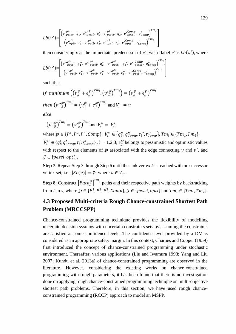
129

𝐿𝑏(𝑣′)=[(𝑣′𝑝𝑒𝑠𝑠𝑖

𝑃1, 𝑞1

′ , 𝑣′𝑝𝑒𝑠𝑠𝑖𝑃2

, 𝑞2′ , 𝑣′𝑝𝑒𝑠𝑠𝑖

𝑃3, 𝑞3

′ , 𝑣′𝑝𝑒𝑠𝑠𝑖𝐶𝑜𝑚𝑝

, 𝑞𝐶𝑜𝑚𝑝′ )

𝑇𝑚𝑙,

(𝑣′𝑜𝑝𝑡𝑖𝑃1

, 𝑟1′, 𝑣′𝑜𝑝𝑡𝑖

𝑃2, 𝑟2

′, 𝑣′𝑜𝑝𝑡𝑖𝑃3

, 𝑟3′, 𝑣′𝑜𝑝𝑡𝑖

𝐶𝑜𝑚𝑝, 𝑟𝐶𝑜𝑚𝑝

′ )𝑇𝑚𝑙

]

then considering 𝑣 as the immediate predecessor of 𝑣′, we re-label 𝑣′as 𝐿𝑏(𝑣′), where

𝐿𝑏(𝑣′)=[(𝑣′′𝑝𝑒𝑠𝑠𝑖

𝑃1, 𝑞1

′′, 𝑣′′𝑝𝑒𝑠𝑠𝑖𝑃2

, 𝑞2′′, 𝑣′′𝑝𝑒𝑠𝑠𝑖

𝑃3, 𝑞3

′′, 𝑣′′𝑝𝑒𝑠𝑠𝑖𝐶𝑜𝑚𝑝

, 𝑞𝐶𝑜𝑚𝑝′′ )

𝑇𝑚𝑙,

(𝑣′′𝑜𝑝𝑡𝑖𝑃1

, 𝑟1′′, 𝑣′′𝑜𝑝𝑡𝑖

𝑃2, 𝑟2

′′, 𝑣′′𝑜𝑝𝑡𝑖𝑃3

, 𝑟3′′, 𝑣′′𝑜𝑝𝑡𝑖

𝐶𝑜𝑚𝑝, 𝑟𝐶𝑜𝑚𝑝

′′ )𝑇𝑚𝑙

]

such that

𝑖𝑓 𝑚𝑖𝑛𝑖𝑚𝑢𝑚 ((𝑣𝒥℘ + 𝑒𝒥

℘)𝑇𝑚𝑙

, (𝑣′𝒥℘)𝑇𝑚𝑙

) = (𝑣𝒥℘ + 𝑒𝒥

℘)𝑇𝑚𝑙

𝑡ℎ𝑒𝑛 (𝑣′′𝒥℘)𝑇𝑚𝑙

= (𝑣𝒥℘ + 𝑒𝒥

℘)𝑇𝑚𝑙

and 𝑉𝑖′′ = 𝑣

𝑒𝑙𝑠𝑒

(𝑣′′𝒥℘)𝑇𝑚𝑙

= (𝑣′𝒥℘)𝑇𝑚𝑙

and 𝑉𝑖′′ = 𝑉𝑖

′,

where ℘ ∈ {𝑃1, 𝑃2, 𝑃3, 𝐶𝑜𝑚𝑝}, 𝑉𝑖′′ ∈ {𝑞𝑖

′′, 𝑞𝐶𝑜𝑚𝑝′′ , 𝑟𝑖

′′, 𝑟𝐶𝑜𝑚𝑝′′ }, 𝑇𝑚𝑙 ∈ {𝑇𝑚1, 𝑇𝑚2},

𝑉𝑖′′ ∈ {𝑞𝑖

′, 𝑞𝐶𝑜𝑚𝑝′ , 𝑟𝑖

′, 𝑟𝐶𝑜𝑚𝑝′ } , 𝑖 = 1,2,3, 𝑒𝒥

℘ belongs to pessimistic and optimistic values

with respect to the elements of ℘ associated with the edge connecting 𝑣 and 𝑣′, and

𝒥 ∈ {𝑝𝑒𝑠𝑠𝑖, 𝑜𝑝𝑡𝑖}.

Step 7: Repeat Step 3 through Step 6 until the sink vertex 𝑡 is reached with no successor

vertex set, i.e., |𝑆𝑟(𝑣)| = ∅, where 𝑣 ∈ 𝑉𝐺.

Step 8: Construct [𝑃𝑎𝑡ℎ𝒥℘]𝑇𝑚𝑙

paths and their respective path weights by backtracking

from 𝑡 to 𝑠, where ℘ ∈ {𝑃1, 𝑃2, 𝑃3, 𝐶𝑜𝑚𝑝}, 𝒥 ∈ {𝑝𝑒𝑠𝑠𝑖, 𝑜𝑝𝑡𝑖} and 𝑇𝑚𝑙 ∈ {𝑇𝑚1, 𝑇𝑚2}.

4.3 Proposed Multi-criteria Rough Chance-constrained Shortest Path

Problem (MRCCSPP)

Chance-constrained programming technique provides the flexibility of modelling

uncertain decision systems with uncertain constraints sets by assuming the constraints

are satisfied at some confidence levels. The confidence level provided by a DM is

considered as an appropriate safety margin. In this context, Charnes and Cooper (1959)

first introduced the concept of chance-constrained programming under stochastic

environment. Thereafter, various applications (Liu and Iwamura 1998; Yang and Liu

2007; Kundu et al. 2013a) of chance-constrained programming are observed in the

literature. However, considering the existing works on chance-constrained

programming with rough parameters, it has been found that there is no investigation

done on applying rough chance-constrained programming technique on multi-objective

shortest path problems. Therefore, in this section, we have used rough chance-

constrained programming (RCCP) approach to model an MSPP.

130

We consider a WCDN, 𝐺(𝑉𝐺 , 𝐸𝐺), where 𝑉𝐺 and 𝐸𝐺 are respectively, the set of vertices

and edges of 𝐺. An edge 𝑒𝑖𝑗 ∈ 𝐸𝐺 , joining a pair of vertices, (𝑣𝑖 , 𝑣𝑗) is associated with

three criteria: distance (𝑃𝑖𝑗1 ), cost (𝑃𝑖𝑗

2) and time (𝑃𝑖𝑗3). Considering these criteria as

rough variables, a model of MSPP is formulated in 𝑀1.

𝑀1:

{

𝑀𝑖𝑛 𝑍1 = ∑ 𝑃𝑖𝑗

1𝑥𝑖𝑗𝑒𝑖𝑗∈𝐸𝐺

𝑀𝑖𝑛 𝑍2 = ∑ 𝑃𝑖𝑗2𝑥𝑖𝑗𝑒𝑖𝑗∈𝐸𝐺

𝑀𝑖𝑛 𝑍3 = ∑ 𝑃𝑖𝑗3𝑥𝑖𝑗𝑒𝑖𝑗∈𝐸𝐺


∑ 𝑥𝑖𝑗 −𝑒𝑖𝑗∈𝐸𝐺∑ 𝑥𝑖𝑗 = {

1 ; 𝑖𝑓 𝑣𝑖 = 𝑠

0 ; 𝑖𝑓 𝑣𝑖 ∉ {𝑠, 𝑡}

−1 ; 𝑖𝑓 𝑣𝑖 = 𝑡 𝑒𝑖𝑗∈𝐸𝐺

𝑥𝑖𝑗 = {1 ; 𝑖𝑓 𝑒𝑖𝑗 ∈ 𝐸𝐺

0 ; 𝑜𝑡ℎ𝑒𝑟𝑤𝑖𝑠𝑒,

(4.1)

where 𝑥𝑖𝑗 is the decision variable, and 𝑠 and 𝑡 are respectively, the source and the sink

vertices of a WCDN. Here, each 𝑃𝑖𝑗𝑘 is expressed as ([𝑃𝑖𝑗

𝑘2, 𝑃𝑖𝑗𝑘3], [𝑃𝑖𝑗

𝑘1, 𝑃𝑖𝑗𝑘4]) such

that 𝑃𝑖𝑗𝑘1 ≤ 𝑃𝑖𝑗

𝑘2 < 𝑃𝑖𝑗𝑘3 ≤ 𝑃𝑖𝑗

𝑘4, 𝑘 = 1,2,3. Since all the criteria: 𝑃𝑖𝑗1 , 𝑃𝑖𝑗

2 and 𝑃𝑖𝑗3 are

considered as rough variables, the objective functions of 𝑀1 shown in (4.1) will also

become rough variables, i.e., 𝑍𝑘 = ([𝑍𝑃𝑘2 , 𝑍

𝑃𝑘3 ], [𝑍

𝑃𝑘1 , 𝑍

𝑃𝑘4 ]), ∀𝑘 ∈ {1, 2, 3}. The

pessimistic and optimistic values of the rough variables are calculated at trust measures

𝑇𝑚1(∈ (0.0,0.5]) and 𝑇𝑚2(∈ (0.5,1.0]) while solving the models of MRCCSPP. The

algorithmic steps to model and solve MRCCSPP by goal attainment method are

presented below.

Input: A WCDN, 𝐺(𝑉𝐺 , 𝐸𝐺), where 𝑉𝐺 and 𝐸𝐺 are the set of vertices and edges such

that for each 𝑣𝑖 , 𝑣𝑗 ∈ 𝑉𝐺 the weights of each edge 𝑒𝑖𝑗 ∈ 𝐸𝐺 are represented by three

criteria: 𝑃𝑖,𝑗1 , 𝑃𝑖,𝑗

2 and 𝑃𝑖,𝑗3 , which are expressed as rough variables, i.e., 𝑃𝑖𝑗

𝑘 =

([𝑃𝑖𝑗𝑘2, 𝑃𝑖𝑗

𝑘3], [𝑃𝑖𝑗𝑘1, 𝑃𝑖𝑗

𝑘4]), 𝑃𝑖𝑗𝑘1 ≤ 𝑃𝑖𝑗


𝑘4, ∀𝑘 = 1,2,3.

Output: Pessimistic and optimistic shortest paths and their corresponding effective

weights with respect to each criterion 𝑃1, 𝑃2 and 𝑃3 of 𝐺, and the compromise

pessimistic and optimistic shortest paths with their corresponding path weights with

respect to all the criteria.

Step 1: Set the trust measure 𝑇𝑚=𝑇𝑚1, where 𝑇𝑚1 ∈ (0.0,0.5].

Step 2: For each criterion 𝑃𝑘 , we formulate and solve the models 𝑀𝑃𝑘𝑟 , 𝑟 = 1,2,3,4,

𝑘 = 1,2,3 as

131

𝑀𝑃𝑘𝑟 :

{

𝑀𝑖𝑛 𝑍𝑃𝑘

𝑟 = ∑ 𝑃𝑖𝑗𝑘𝑟𝑥𝑖𝑗𝑒𝑖𝑗∈𝐸𝐺


𝑐𝑜𝑛𝑠𝑡𝑟𝑎𝑖𝑛𝑡𝑠 𝑜𝑓 (4.1) 𝑘 = 1,2,3, 𝑟 = 1,2,3,4.

(4.2)

Step 3: To find the pessimistic shortest paths and their corresponding path weights,

formulate a rough chance-constrained model of 𝑀1 to minimize the smallest objectives

𝑍1, 𝑍2 and 𝑍3 with respect to 𝑃1, 𝑃2 and 𝑃3 satisfying 𝑇𝑟{𝑍𝑘 ≤ 𝑍𝑘} ≥ 𝑇𝑚, where the

value of 𝑇𝑚 is the predetermined confidence level (trust level) set by the decision

maker. Accordingly, the following model minimizes the 𝑇𝑚-pessimistic value,

(𝑍𝑘)𝑝𝑒𝑠𝑠𝑖𝑇𝑚 of 𝑍𝑘, 𝑘 = 1,2,3.

𝑀𝑘+1:

{

𝑀𝑖𝑛(𝑀𝑖𝑛 𝑍𝑘)


𝑇𝑟{𝑍𝑘 ≤ 𝑍𝑘} ≥ 𝑇𝑚

𝑤𝑖𝑡ℎ 𝑐𝑜𝑛𝑠𝑡𝑟𝑎𝑖𝑛𝑡𝑠 𝑜𝑓 (4.1) ∀ 𝑘 ∈ {1,2,3}.

(4.3)

Step 4: Following the definition of 𝑇𝑚-pessimistic value of a rough variable (cf.

Definition 1.3.21), the crisp equivalent of the rough CCM of Step 3 becomes

𝑀𝑘+4:

{

𝑀𝑖𝑛 ((𝑍𝑘)𝑝𝑒𝑠𝑠𝑖𝑇𝑚 ) =

{

(1 − 2𝑇𝑚)𝑍

𝑃𝑘1 + 2𝑇𝑚 𝑍

𝑃𝑘4 ; 𝑖𝑓 𝑇𝑚 ≤ (

𝑍𝑃𝑘2 −𝑍

𝑃𝑘1

2(𝑍𝑃𝑘4 −𝑍

𝑃𝑘1 )) (4.4)

2(1 − 𝑇𝑚)𝑍𝑃𝑘1 + (2𝑇𝑚 − 1)𝑍

𝑃𝑘4 ; 𝑖𝑓 𝑇𝑚 ≥ (

𝑍𝑃𝑘3 +𝑍

𝑃𝑘4 −2𝑍

𝑃𝑘1


𝑃𝑘1 )

)

𝑍𝑃𝑘1 (𝑍

𝑃𝑘3 −𝑍

𝑃𝑘2 )+𝑍

𝑃𝑘2 (𝑍

𝑃𝑘4 −𝑍

𝑃𝑘1 )+(2𝑇𝑚(𝑍

𝑃𝑘3 −𝑍

𝑃𝑘2 )×(𝑍

𝑃𝑘4 −𝑍

𝑃𝑘1 ))

(𝑍𝑃𝑘3 −𝑍

𝑃𝑘2 )+(𝑍

𝑃𝑘4 −𝑍

𝑃𝑘1 )

; 𝑜𝑡ℎ𝑒𝑟𝑤𝑖𝑠𝑒


𝑡ℎ𝑒 𝑐𝑜𝑛𝑠𝑡𝑟𝑎𝑖𝑛𝑡𝑠 𝑜𝑓 (4.1) ∀ 𝑘 ∈ {1,2,3}.

Step 5: To find the optimistic shortest paths and their corresponding path weights,

formulate a rough chance-constrained model of 𝑀1 to minimize the greatest objectives

𝑍1, 𝑍2 and 𝑍3 with respect to 𝑃1, 𝑃2 and 𝑃3 satisfying 𝑇𝑟 {𝑍𝑘 ≥ 𝑍𝑘} ≥ 𝑇𝑚 at trust

level, 𝑇𝑚, i.e., we minimize the 𝑇𝑚-optimistic value, (𝑍𝑘)𝑜𝑝𝑡𝑖𝑇𝑚 of 𝑍𝑘, 𝑘 = 1,2,3.

𝑀𝑘+7:

{

𝑀𝑖𝑛 (𝑀𝑎𝑥 𝑍𝑘)


𝑇𝑟 {𝑍𝑘 ≥ 𝑍𝑘} ≥ 𝑇𝑚

𝑤𝑖𝑡ℎ 𝑡ℎ𝑒 𝑐𝑜𝑛𝑠𝑡𝑟𝑎𝑖𝑛𝑡𝑠 𝑜𝑓 (4.1) ∀ 𝑘 ∈ {1,2,3}.

(4.5)

132

Step 6: From the definition of 𝑇𝑚-optimistic value (cf. Definition 1.3.21), the crisp

equivalent of the rough chance-constrained model of Step 5 becomes

𝑀𝑘+10:

{

𝑀𝑖𝑛 ((𝑍𝑘)𝑜𝑝𝑡𝑖𝑇𝑚 ) =

{

(1 − 2𝑇𝑚)𝑍

𝑃𝑘4 + 2𝑇𝑚 𝑍

𝑃𝑘1 ; 𝑖𝑓 𝑇𝑚 ≤ (

𝑍𝑃𝑘4 −𝑍

𝑃𝑘3


𝑃𝑘1 )) (4.6)

2(1 − 𝑇𝑚)𝑍𝑃𝑘4 + (2𝑇𝑚− 1)𝑍

𝑃𝑘1 ; 𝑖𝑓 𝑇𝑚 ≥ (

2𝑍𝑃𝑘4 −𝑍

𝑃𝑘2 −𝑍

𝑃𝑘1


𝑃𝑘1 )

)

𝑍𝑃𝑘4 (𝑍

𝑃𝑘3 −𝑍

𝑃𝑘2 )+𝑍

𝑃𝑘3 (𝑍

𝑃𝑘4 −𝑍

𝑃𝑘1 )−(2𝑇𝑚(𝑍

𝑃𝑘3 −𝑍

𝑃𝑘2 )×(𝑍

𝑃𝑘4 −𝑍

𝑃𝑘1 ))

(𝑍𝑃𝑘3 −𝑍

𝑃𝑘2 )+(𝑍

𝑃𝑘4 −𝑍

𝑃𝑘1 )

; 𝑜𝑡ℎ𝑒𝑟𝑤𝑖𝑠𝑒


𝑐𝑜𝑛𝑠𝑡𝑟𝑎𝑖𝑛𝑡𝑠 𝑜𝑓 (4.1) ∀ 𝑘 ∈ {1,2,3}.

Step 7: Calculate the argument-dependent OWA weights (Z. Xu 2006) (cf. Section

1.3.12 and Example 1.3.15) of 𝑇𝑚-pessimistic and 𝑇𝑚-optimistic objective vectors

using Step 7.1 through Step 7.4.

Step 7.1: For 𝑇𝑚-pessimistic and 𝑇𝑚-optimistic objective vectors calculate the means,

𝜇𝑝𝑒𝑠𝑠𝑖𝑇𝑚 and 𝜇𝑜𝑝𝑡𝑖

𝑇𝑚 for the objective vectors, 𝛾𝑝𝑒𝑠𝑠𝑖= [(𝑍1)𝑝𝑒𝑠𝑠𝑖𝑇𝑚 , (𝑍2)𝑝𝑒𝑠𝑠𝑖

𝑇𝑚 , (𝑍3)𝑝𝑒𝑠𝑠𝑖𝑇𝑚 ]

and 𝛾𝑜𝑝𝑡𝑖= [(𝑍1)𝑜𝑝𝑡𝑖𝑇𝑚 , (𝑍2)𝑜𝑝𝑡𝑖

𝑇𝑚 , (𝑍3)𝑜𝑝𝑡𝑖𝑇𝑚 ], respectively, where 𝜇𝑝𝑒𝑠𝑠𝑖

𝑇𝑚 = 1

3∑ (𝑍𝑘)𝑝𝑒𝑠𝑠𝑖

𝑇𝑚3𝑘=1

and 𝜇𝑜𝑝𝑡𝑖𝑇𝑚 =

1

3∑ (𝑍𝑘)𝑜𝑝𝑡𝑖

𝑇𝑚3𝑘=1 .

Step 7.2: Let {𝜑(1), 𝜑(2), 𝜑(3)} be a permutation of (1,2,3) such that 𝛾𝒥′ =

[(𝑍𝜑(1))𝒥𝑇𝑚, (𝑍𝜑(2))𝒥

𝑇𝑚, (𝑍𝜑(3))𝒥

𝑇𝑚] be a permutation of 𝛾𝒥, where (𝑍𝜑(𝑡−1))𝒥

𝑇𝑚≥

(𝑍𝜑(𝑡))𝒥𝑇𝑚∀ 𝑡 ∈ {2,3} and 𝒥 ∈ {𝑝𝑒𝑠𝑠𝑖, 𝑜𝑝𝑡𝑖}.

Step 7.3: Calculate the similarity degree, 𝑠 ((𝑍𝜑(𝑘))𝒥𝑇𝑚, 𝜇𝒥𝑇𝑚) with respect to 𝑘𝑡ℎ

largest objective of 𝛾𝒥′ and the corresponding mean, so that 𝑠 ((𝑍𝜑(𝑘))𝒥

𝑇𝑚, 𝜇𝒥𝑇𝑚) = 1 −

|((𝑍𝜑(𝑘))𝑝𝑒𝑠𝑠𝑖

𝑇𝑚−𝜇𝒥

𝑇𝑚)|

∑ |((𝑍𝑘)𝒥𝑇𝑚−𝜇𝒥

𝑇𝑚)|3𝑘=1

∀ 𝑘 ∈ {1,2,3} and 𝒥 ∈ {𝑝𝑒𝑠𝑠𝑖, 𝑜𝑝𝑡𝑖}.

Step 7.4: Determine the corresponding pessimistic and optimistic weight vectors,

(𝒥 = [(1)𝒥, (2)𝒥, (3)𝒥]𝑇) such that, (𝑘)𝒥 =

𝑠((𝑍𝜑(𝑘))𝒥

𝑇𝑚, 𝜇𝒥

𝑇𝑚)

∑ 𝑠((𝑍𝜑(𝑘))𝒥

𝑇𝑚, 𝜇𝒥

𝑇𝑚)3𝑘=1

, 𝑘 = 1,2,3,

where (𝑘)𝒥 ∈ [0,1] and 𝒥 ∈ {𝑝𝑒𝑠𝑠𝑖, 𝑜𝑝𝑡𝑖}.

Step 8: For the weight vectors, 𝑝𝑒𝑠𝑠𝑖 and 𝑜𝑝𝑡𝑖 the pessimistic and optimistic

compromise models of 𝑀𝑘+4 and 𝑀𝑘+10, 𝑘 = 1,2,3 correspondingly becomes 𝑀′ and

𝑀′′, as presented below.

133

𝑀′:

{

𝑀𝑖𝑛 𝛿1


(𝑍𝑘)𝑝𝑒𝑠𝑠𝑖𝑇𝑚 − (𝑘)𝑝𝑒𝑠𝑠𝑖𝛿1 ≤ ((𝑍𝑘)𝑝𝑒𝑠𝑠𝑖

𝑇𝑚 )∗


∀(𝑘)𝑝𝑒𝑠𝑠𝑖 ∈ [0,1], 𝑘 = 1,2,3

(4.7)

𝑀′′:

{

𝑀𝑖𝑛 𝛿2


(𝑍𝑘)𝑜𝑝𝑡𝑖𝑇𝑚 − (𝑘)𝑜𝑝𝑡𝑖𝛿2 ≤ ((𝑍𝑘)𝑜𝑝𝑡𝑖

𝑇𝑚 )∗


∀(𝑘)𝑜𝑝𝑡𝑖 ∈ [0,1], 𝑘 = 1,2,3,

(4.8)

where ((𝑍𝑘)𝑝𝑒𝑠𝑠𝑖𝑇𝑚 )

∗and ((𝑍𝑘)𝑜𝑝𝑡𝑖

𝑇𝑚 )∗ are the goals associated with each of the objectives

(𝑍𝑘)𝑝𝑒𝑠𝑠𝑖𝑇𝑚 and (𝑍𝑘)𝑜𝑝𝑡𝑖

𝑇𝑚 , respectively ∀ 𝑘 ∈ {1, 2, 3}. In our study, these goals are

obtained by solving each objective of 𝑀𝑘+4 and 𝑀𝑘+10, 𝑘 = 1,2,3 individually. The

compromise models in (4.7) and (4.8) are formulated using goal attainment method (cf.

Section 1.3.15.3). Subsequently, we determine the compromise objective vectors,

(𝑍)𝑝𝑒𝑠𝑠𝑖𝑇𝑚 = [

(𝑍1)𝑝𝑒𝑠𝑠𝑖𝑇𝑚



] and (𝑍)𝑜𝑝𝑡𝑖𝑇𝑚 = [

(𝑍1)𝑜𝑝𝑡𝑖𝑇𝑚



] by solving the models 𝑀′ and 𝑀′′,

respectively.

Step 9: Set 𝑇𝑚=𝑇𝑚2, where 𝑇𝑚2 ∈ (0.5,1.0] and repeat Step 3 through Step 8.

4.4 Numerical Illustration

In this section, we have considered a WCDN 𝐺(𝑉𝐺 , 𝐸𝐺) depicted in Fig. 4.1. 𝑉𝐺 and 𝐸𝐺

are respectively, the set of vertices and edges of 𝐺. The weights of each edge 𝑒𝑖𝑗 ∈

𝐸𝐺 are represented by three criteria: distance (𝑃𝑖𝑗1), cost (𝑃𝑖𝑗

2) and time (𝑃𝑖𝑗3). Each of

these criterion is expressed as rough variable, i.e., 𝑃𝑖𝑗𝑘 = ([𝑃𝑖𝑗

𝑘2, 𝑃𝑖𝑗𝑘3], [𝑃𝑖𝑗

𝑘1, 𝑃𝑖𝑗𝑘4]), 𝑘 =

{1,2,3} so that 𝑃𝑖𝑗𝑘1 ≤ 𝑃𝑖𝑗


𝑘4. Vertices, 𝑣1 and 𝑣11 of 𝐺 are respectively,

designated as source (𝑠) and sink (𝑡) vertices. The edge weights of 𝐺 are presented in

Table 4.1.

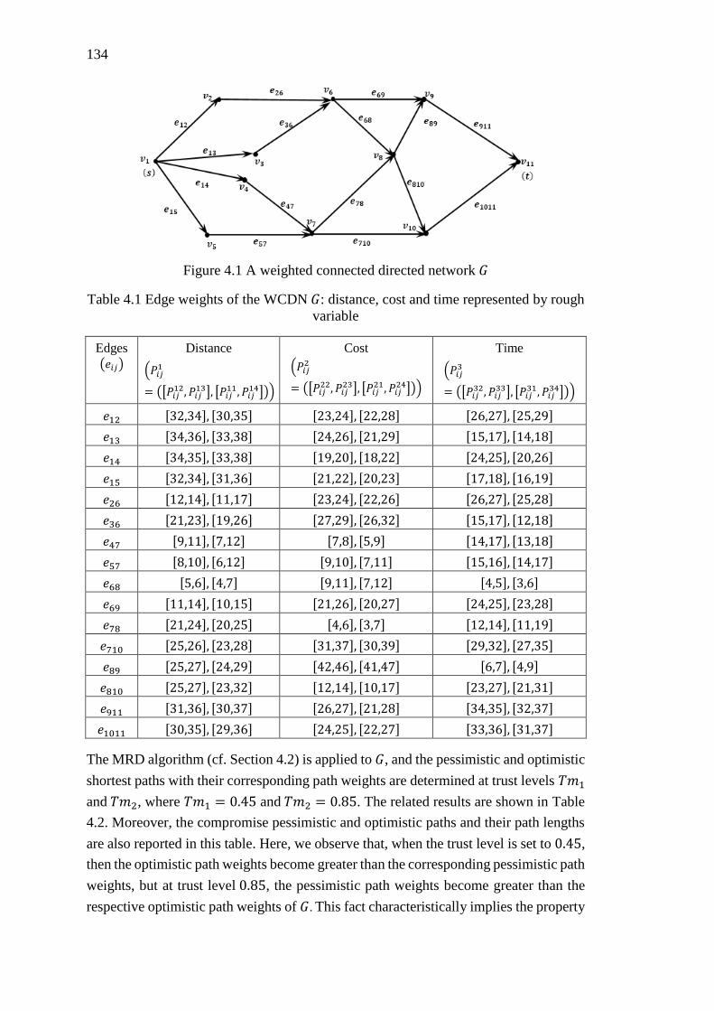
134

Figure 4.1 A weighted connected directed network 𝐺

Table 4.1 Edge weights of the WCDN 𝐺: distance, cost and time represented by rough

variable

The MRD algorithm (cf. Section 4.2) is applied to 𝐺, and the pessimistic and optimistic

shortest paths with their corresponding path weights are determined at trust levels 𝑇𝑚1

and 𝑇𝑚2, where 𝑇𝑚1 = 0.45 and 𝑇𝑚2 = 0.85. The related results are shown in Table

4.2. Moreover, the compromise pessimistic and optimistic paths and their path lengths

are also reported in this table. Here, we observe that, when the trust level is set to 0.45,

then the optimistic path weights become greater than the corresponding pessimistic path

weights, but at trust level 0.85, the pessimistic path weights become greater than the

respective optimistic path weights of 𝐺. This fact characteristically implies the property

Edges

(𝑒𝑖𝑗)

Distance

(𝑃𝑖𝑗1

= ([𝑃𝑖𝑗12, 𝑃𝑖𝑗

13], [𝑃𝑖𝑗11, 𝑃𝑖𝑗

14]))

Cost

(𝑃𝑖𝑗2


23], [𝑃𝑖𝑗21, 𝑃𝑖𝑗

24]))

Time

(𝑃𝑖𝑗3


33], [𝑃𝑖𝑗31, 𝑃𝑖𝑗

34]))

𝑒12 [32,34], [30,35] [23,24], [22,28] [26,27], [25,29]

𝑒13 [34,36], [33,38] [24,26], [21,29] [15,17], [14,18]

𝑒14 [34,35], [33,38] [19,20], [18,22] [24,25], [20,26]

𝑒15 [32,34], [31,36] [21,22], [20,23] [17,18], [16,19]

𝑒26 [12,14], [11,17] [23,24], [22,26] [26,27], [25,28]

𝑒36 [21,23], [19,26] [27,29], [26,32] [15,17], [12,18]

𝑒47 [9,11], [7,12] [7,8], [5,9] [14,17], [13,18]

𝑒57 [8,10], [6,12] [9,10], [7,11] [15,16], [14,17]

𝑒68 [5,6], [4,7] [9,11], [7,12] [4,5], [3,6]

𝑒69 [11,14], [10,15] [21,26], [20,27] [24,25], [23,28]

𝑒78 [21,24], [20,25] [4,6], [3,7] [12,14], [11,19]

𝑒710 [25,26], [23,28] [31,37], [30,39] [29,32], [27,35]

𝑒89 [25,27], [24,29] [42,46], [41,47] [6,7], [4,9]

𝑒810 [25,27], [23,32] [12,14], [10,17] [23,27], [21,31]

𝑒911 [31,36], [30,37] [26,27], [21,28] [34,35], [32,37]

𝑒1011 [30,35], [29,36] [24,25], [22,27] [33,36], [31,37]

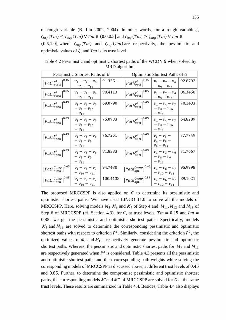
135

of rough variable (B. Liu 2002, 2004). In other words, for a rough variable 휁,

휁𝑖𝑛𝑓(𝑇𝑚) ≤ 휁𝑠𝑢𝑝(𝑇𝑚) ∀ 𝑇𝑚 ∈ (0.0,0.5] and 휁𝑖𝑛𝑓(𝑇𝑚) ≥ 휁𝑠𝑢𝑝(𝑇𝑚) ∀ 𝑇𝑚 ∈

(0.5,1.0], where 휁𝑖𝑛𝑓(𝑇𝑚) and 휁𝑠𝑢𝑝(𝑇𝑚) are respectively, the pessimistic and

optimistic values of 휁, and 𝑇𝑚 is its trust level.

Table 4.2 Pessimistic and optimistic shortest paths of the WCDN 𝐺 when solved by

MRD algorithm

Pessimistic Shortest Paths of 𝐺 Optimistic Shortest Paths of 𝐺

[𝑃𝑎𝑡ℎ𝑝𝑒𝑠𝑠𝑖𝑃1 ]

0.45 𝑣1 − 𝑣2 − 𝑣6− 𝑣9 − 𝑣11

91.3351 [𝑃𝑎𝑡ℎ𝑜𝑝𝑡𝑖

𝑃1 ]0.45

𝑣1 − 𝑣2 − 𝑣6− 𝑣9 − 𝑣11

92.8792


0.85 𝑣1 − 𝑣2 − 𝑣6− 𝑣9 − 𝑣11


𝑃1 ]0.85

𝑣1 − 𝑣2 − 𝑣6− 𝑣9 − 𝑣11

86.3458


0.45 𝑣1 − 𝑣4 − 𝑣7− 𝑣8 − 𝑣10− 𝑣11


𝑃2 ]0.45

𝑣1 − 𝑣4 − 𝑣7− 𝑣8 − 𝑣10− 𝑣11

70.1433


0.85 𝑣1 − 𝑣4 − 𝑣7− 𝑣8 − 𝑣10− 𝑣11


𝑃2 ]0.85

𝑣1 − 𝑣4 − 𝑣7− 𝑣8 − 𝑣10− 𝑣11

64.8289


0.45 𝑣1 − 𝑣3 − 𝑣6− 𝑣8 − 𝑣9− 𝑣11


𝑃3 ]0.45

𝑣1 − 𝑣3 −𝑣6 − 𝑣8 −𝑣9 − 𝑣11

77.7749


0.85 𝑣1 − 𝑣3 − 𝑣6− 𝑣8 − 𝑣9− 𝑣11


𝑃3 ]0.85

𝑣1 − 𝑣3 − 𝑣6− 𝑣8 − 𝑣9− 𝑣11

71.7667

[𝑃𝑎𝑡ℎ𝑝𝑒𝑠𝑠𝑖𝐶𝑜𝑚𝑝

]0.45

𝑣1 − 𝑣5 − 𝑣7− 𝑣10 − 𝑣11

94.7430 [𝑃𝑎𝑡ℎ𝑜𝑝𝑡𝑖𝐶𝑜𝑚𝑝

]0.45

𝑣1 − 𝑣5 − 𝑣7− 𝑣10 − 𝑣11

95.9998

[𝑃𝑎𝑡ℎ𝑝𝑒𝑠𝑠𝑖𝐶𝑜𝑚𝑝

]0.85

𝑣1 − 𝑣5 − 𝑣7− 𝑣10 − 𝑣11

100.4138 [𝑃𝑎𝑡ℎ𝑜𝑝𝑡𝑖𝐶𝑜𝑚𝑝

]0.85

𝑣1 − 𝑣5 − 𝑣7− 𝑣10 − 𝑣11

89.1021

The proposed MRCCSPP is also applied on 𝐺 to determine its pessimistic and

optimistic shortest paths. We have used LINGO 11.0 to solve all the models of

MRCCSPP. Here, solving models 𝑀5, 𝑀6 and 𝑀7 of Step 4 and 𝑀11, 𝑀12 and 𝑀13 of

Step 6 of MRCCSPP (cf. Section 4.3), for 𝐺, at trust levels, 𝑇𝑚 = 0.45 and 𝑇𝑚 =

0.85, we get the pessimistic and optimistic shortest paths. Specifically, models

𝑀5 and 𝑀11 are solved to determine the corresponding pessimistic and optimistic

shortest paths with respect to criterion 𝑃1. Similarly, considering the criterion 𝑃2, the

optimized values of 𝑀6 and 𝑀12, respectively generate pessimistic and optimistic

shortest paths. Whereas, the pessimistic and optimistic shortest paths for 𝑀7 and 𝑀13

are respectively generated when 𝑃3 is considered. Table 4.3 presents all the pessimistic

and optimistic shortest paths and their corresponding path weights while solving the

corresponding models of MRCCSPP as discussed above, at different trust levels of 0.45

and 0.85. Further, to determine the compromise pessimistic and optimistic shortest

paths, the corresponding models 𝑀′and 𝑀′′ of MRCCSPP are solved for 𝐺 at the same

trust levels. These results are summarized in Table 4.4. Besides, Table 4.4 also displays

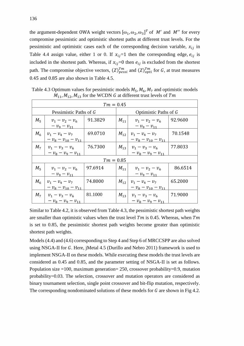
136

the argument-dependent OWA weight vectors [1,2,3]𝑇 of 𝑀′ and 𝑀′′ for every

compromise pessimistic and optimistic shortest paths at different trust levels. For the

pessimistic and optimistic cases each of the corresponding decision variable, 𝑥𝑖𝑗 in

Table 4.4 assign value, either 1 or 0. If 𝑥𝑖𝑗=1 then the corresponding edge, 𝑒𝑖𝑗 is

included in the shortest path. Whereas, if 𝑥𝑖𝑗=0 then 𝑒𝑖𝑗 is excluded from the shortest

path. The compromise objective vectors, (𝑍)𝑝𝑒𝑠𝑠𝑖𝑇𝑚 and (𝑍)𝑜𝑝𝑡𝑖

𝑇𝑚 for 𝐺, at trust measures

0.45 and 0.85 are also shown in Table 4.5.

Table 4.3 Optimum values for pessimistic models 𝑀5, 𝑀6, 𝑀7 and optimistic models

𝑀11, 𝑀12, 𝑀13 for the WCDN 𝐺 at different trust levels of 𝑇𝑚

𝑇𝑚 = 0.45

Pessimistic Paths of 𝐺 Optimistic Paths of 𝐺

𝑀5 𝑣1 − 𝑣2 − 𝑣6− 𝑣9 − 𝑣11

91.3829 𝑀11 𝑣1 − 𝑣2 − 𝑣6− 𝑣9 − 𝑣11

92.9600

𝑀6 𝑣1 − 𝑣4 − 𝑣7− 𝑣8 − 𝑣10 − 𝑣11

69.0710 𝑀12 𝑣1 − 𝑣4 − 𝑣7− 𝑣8 − 𝑣10 − 𝑣11

70.1548

𝑀7 𝑣1 − 𝑣3 − 𝑣6− 𝑣8 − 𝑣9 − 𝑣11

76.7300 𝑀13 𝑣1 − 𝑣3 − 𝑣6− 𝑣8 − 𝑣9 − 𝑣11

77.8033

𝑇𝑚 = 0.85

𝑀5 𝑣1 − 𝑣2 − 𝑣6− 𝑣9 − 𝑣11

97.6914 𝑀11 𝑣1 − 𝑣2 − 𝑣6− 𝑣9 − 𝑣11

86.6514

𝑀6 𝑣1 − 𝑣4 − 𝑣7− 𝑣8 − 𝑣10 − 𝑣11

74.8000 𝑀12 𝑣1 − 𝑣4 − 𝑣7− 𝑣8 − 𝑣10 − 𝑣11

65.2000

𝑀7 𝑣1 − 𝑣3 − 𝑣6− 𝑣8 − 𝑣9 − 𝑣11

81.1000 𝑀13 𝑣1 − 𝑣3 − 𝑣6− 𝑣8 − 𝑣9 − 𝑣11

71.9000

Similar to Table 4.2, it is observed from Table 4.3, the pessimistic shortest path weights

are smaller than optimistic values when the trust level 𝑇𝑚 is 0.45. Whereas, when 𝑇𝑚

is set to 0.85, the pessimistic shortest path weights become greater than optimistic

shortest path weights.

Models (4.4) and (4.6) corresponding to Step 4 and Step 6 of MRCCSPP are also solved

using NSGA-II for 𝐺. Here, jMetal 4.5 (Durillo and Nebro 2011) framework is used to

implement NSGA-II on these models. While executing these models the trust levels are

considered as 0.45 and 0.85, and the parameter setting of NSGA-II is set as follows.

Population size =100, maximum generation= 250, crossover probability=0.9, mutation

probability=0.03. The selection, crossover and mutation operators are considered as

binary tournament selection, single point crossover and bit-flip mutation, respectively.

The corresponding nondominated solutions of these models for 𝐺 are shown in Fig 4.2.

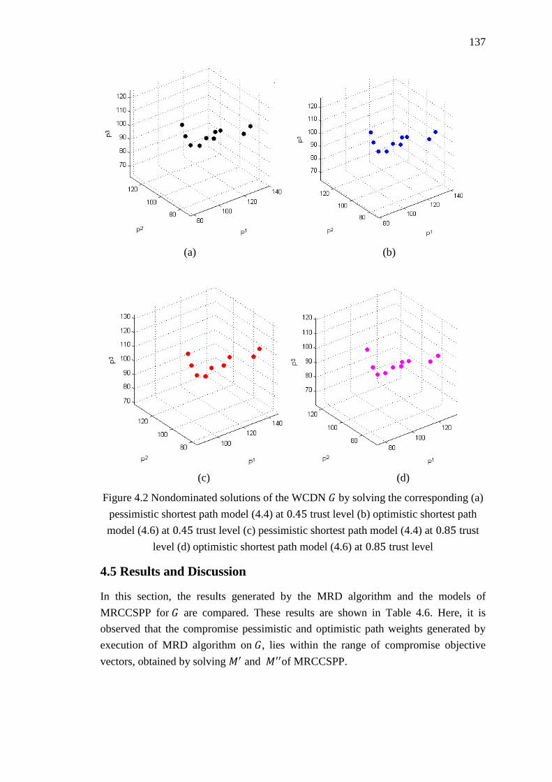
137

(a) (b)

(c) (d)

Figure 4.2 Nondominated solutions of the WCDN 𝐺 by solving the corresponding (a)

pessimistic shortest path model (4.4) at 0.45 trust level (b) optimistic shortest path

model (4.6) at 0.45 trust level (c) pessimistic shortest path model (4.4) at 0.85 trust

level (d) optimistic shortest path model (4.6) at 0.85 trust level


In this section, the results generated by the MRD algorithm and the models of

MRCCSPP for 𝐺 are compared. These results are shown in Table 4.6. Here, it is

observed that the compromise pessimistic and optimistic path weights generated by

execution of MRD algorithm on 𝐺, lies within the range of compromise objective

vectors, obtained by solving 𝑀′ and 𝑀′′of MRCCSPP.

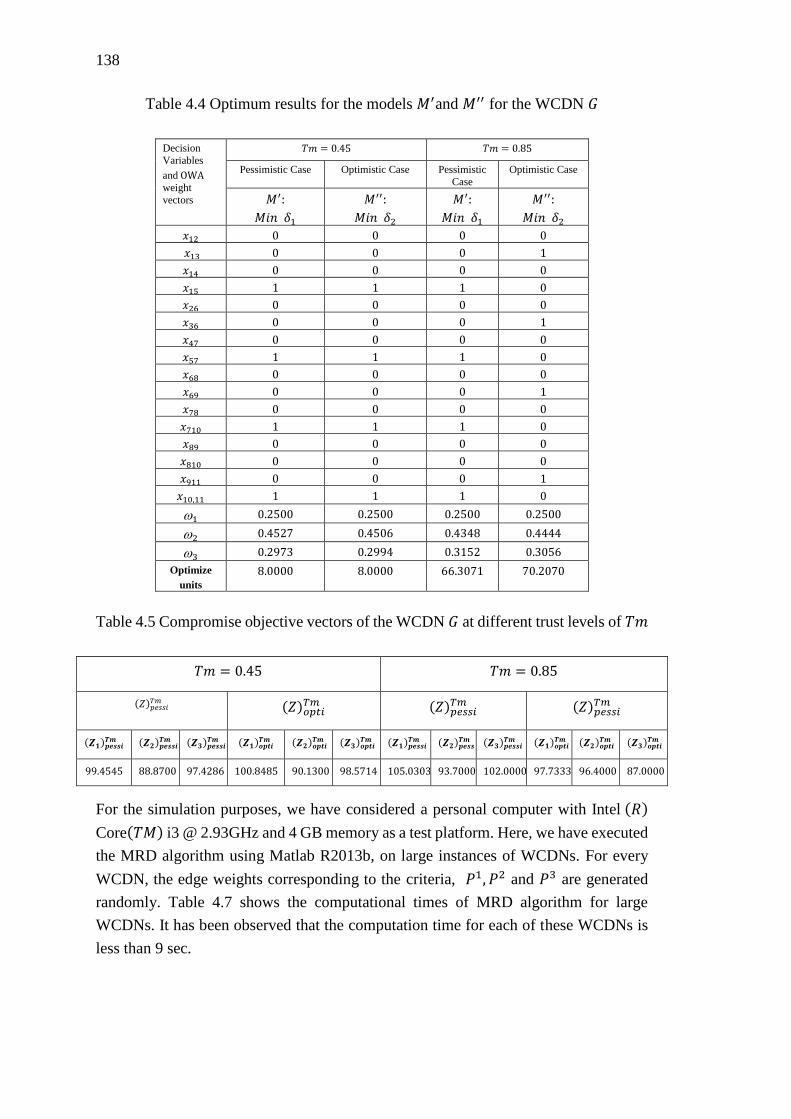
138

Table 4.4 Optimum results for the models 𝑀′and 𝑀′′ for the WCDN 𝐺

Table 4.5 Compromise objective vectors of the WCDN 𝐺 at different trust levels of 𝑇𝑚

For the simulation purposes, we have considered a personal computer with Intel (𝑅)

Core(𝑇𝑀) i3 @ 2.93GHz and 4 GB memory as a test platform. Here, we have executed

the MRD algorithm using Matlab R2013b, on large instances of WCDNs. For every

WCDN, the edge weights corresponding to the criteria, 𝑃1, 𝑃2 and 𝑃3 are generated

randomly. Table 4.7 shows the computational times of MRD algorithm for large

WCDNs. It has been observed that the computation time for each of these WCDNs is

less than 9 sec.

Decision

Variables

and OWA

weight

vectors

𝑇𝑚 = 0.45 𝑇𝑚 = 0.85

Pessimistic Case Optimistic Case Pessimistic

Case

Optimistic Case

𝑀′:

𝑀𝑖𝑛 𝛿1

𝑀′′:

𝑀𝑖𝑛 𝛿2

𝑀′:

𝑀𝑖𝑛 𝛿1

𝑀′′:

𝑀𝑖𝑛 𝛿2 𝑥12 0 0 0 0

𝑥13 0 0 0 1

𝑥14 0 0 0 0

𝑥15 1 1 1 0

𝑥26 0 0 0 0

𝑥36 0 0 0 1

𝑥47 0 0 0 0

𝑥57 1 1 1 0

𝑥68 0 0 0 0

𝑥69 0 0 0 1

𝑥78 0 0 0 0

𝑥710 1 1 1 0

𝑥89 0 0 0 0

𝑥810 0 0 0 0

𝑥911 0 0 0 1

𝑥10,11 1 1 1 0

1 0.2500 0.2500 0.2500 0.2500

2 0.4527 0.4506 0.4348 0.4444

3 0.2973 0.2994 0.3152 0.3056

Optimize

units

8.0000 8.0000 66.3071 70.2070

𝑇𝑚 = 0.45 𝑇𝑚 = 0.85

(𝑍)𝑝𝑒𝑠𝑠𝑖𝑇𝑚 (𝑍)𝑜𝑝𝑡𝑖

𝑇𝑚 (𝑍)𝑝𝑒𝑠𝑠𝑖𝑇𝑚 (𝑍)𝑝𝑒𝑠𝑠𝑖

𝑇𝑚

(𝒁𝟏)𝒑𝒆𝒔𝒔𝒊𝑻𝒎 (𝒁𝟐)𝒑𝒆𝒔𝒔𝒊

𝑻𝒎 (𝒁𝟑)𝒑𝒆𝒔𝒔𝒊𝑻𝒎 (𝒁𝟏)𝒐𝒑𝒕𝒊

𝑻𝒎 (𝒁𝟐)𝒐𝒑𝒕𝒊𝑻𝒎 (𝒁𝟑)𝒐𝒑𝒕𝒊

𝑻𝒎 (𝒁𝟏)𝒑𝒆𝒔𝒔𝒊𝑻𝒎 (𝒁𝟐)𝒑𝒆𝒔𝒔𝒊

𝑻𝒎 (𝒁𝟑)𝒑𝒆𝒔𝒔𝒊𝑻𝒎 (𝒁𝟏)𝒐𝒑𝒕𝒊

𝑻𝒎 (𝒁𝟐)𝒐𝒑𝒕𝒊𝑻𝒎 (𝒁𝟑)𝒐𝒑𝒕𝒊

𝑻𝒎

99.4545 88.8700 97.4286 100.8485 90.1300 98.5714 105.0303 93.7000 102.0000 97.7333 96.4000 87.0000

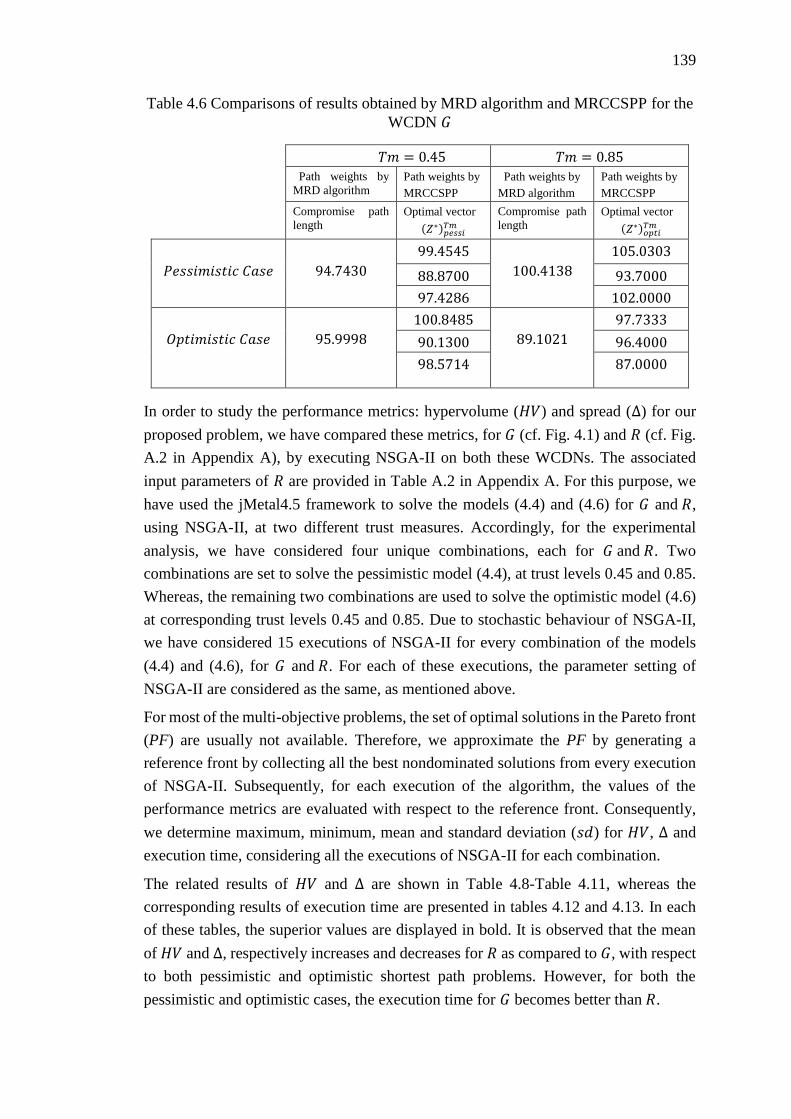
139

Table 4.6 Comparisons of results obtained by MRD algorithm and MRCCSPP for the

WCDN 𝐺

𝑇𝑚 = 0.45 𝑇𝑚 = 0.85

Path weights by

MRD algorithm

Path weights by

MRCCSPP

Path weights by

MRD algorithm

Path weights by

MRCCSPP

Compromise path

length

Optimal vector

(𝑍∗)𝑝𝑒𝑠𝑠𝑖𝑇𝑚

Compromise path

length

Optimal vector

(𝑍∗)𝑜𝑝𝑡𝑖𝑇𝑚

𝑃𝑒𝑠𝑠𝑖𝑚𝑖𝑠𝑡𝑖𝑐 𝐶𝑎𝑠𝑒

94.7430

99.4545

100.4138

105.0303

88.8700 93.7000

97.4286 102.0000

𝑂𝑝𝑡𝑖𝑚𝑖𝑠𝑡𝑖𝑐 𝐶𝑎𝑠𝑒

95.9998

100.8485

89.1021

97.7333

90.1300 96.4000

98.5714 87.0000

In order to study the performance metrics: hypervolume (𝐻𝑉) and spread (Δ) for our

proposed problem, we have compared these metrics, for 𝐺 (cf. Fig. 4.1) and 𝑅 (cf. Fig.

A.2 in Appendix A), by executing NSGA-II on both these WCDNs. The associated

input parameters of 𝑅 are provided in Table A.2 in Appendix A. For this purpose, we

have used the jMetal4.5 framework to solve the models (4.4) and (4.6) for 𝐺 and 𝑅,

using NSGA-II, at two different trust measures. Accordingly, for the experimental

analysis, we have considered four unique combinations, each for 𝐺 and 𝑅. Two

combinations are set to solve the pessimistic model (4.4), at trust levels 0.45 and 0.85.

Whereas, the remaining two combinations are used to solve the optimistic model (4.6)

at corresponding trust levels 0.45 and 0.85. Due to stochastic behaviour of NSGA-II,

we have considered 15 executions of NSGA-II for every combination of the models

(4.4) and (4.6), for 𝐺 and 𝑅. For each of these executions, the parameter setting of

NSGA-II are considered as the same, as mentioned above.

For most of the multi-objective problems, the set of optimal solutions in the Pareto front

(PF) are usually not available. Therefore, we approximate the PF by generating a

reference front by collecting all the best nondominated solutions from every execution

of NSGA-II. Subsequently, for each execution of the algorithm, the values of the

performance metrics are evaluated with respect to the reference front. Consequently,

we determine maximum, minimum, mean and standard deviation (𝑠𝑑) for 𝐻𝑉, Δ and

execution time, considering all the executions of NSGA-II for each combination.

The related results of 𝐻𝑉 and Δ are shown in Table 4.8-Table 4.11, whereas the

corresponding results of execution time are presented in tables 4.12 and 4.13. In each

of these tables, the superior values are displayed in bold. It is observed that the mean

of 𝐻𝑉 and Δ, respectively increases and decreases for 𝑅 as compared to 𝐺, with respect

to both pessimistic and optimistic shortest path problems. However, for both the

pessimistic and optimistic cases, the execution time for 𝐺 becomes better than 𝑅.

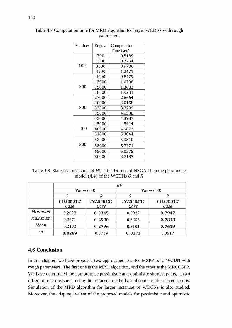
140

Table 4.7 Computation time for MRD algorithm for larger WCDNs with rough

parameters

Table 4.8 Statistical measures of 𝐻𝑉 after 15 runs of NSGA-II on the pessimistic

model (4.4) of the WCDNs 𝐺 and 𝑅

𝐻𝑉

𝑇𝑚 = 0.45 𝑇𝑚 = 0.85

𝐺 𝑅 𝐺 𝑅

𝑃𝑒𝑠𝑠𝑖𝑚𝑖𝑠𝑡𝑖𝑐

𝐶𝑎𝑠𝑒 𝑃𝑒𝑠𝑠𝑖𝑚𝑖𝑠𝑡𝑖𝑐

𝐶𝑎𝑠𝑒


𝐶𝑎𝑠𝑒


𝐶𝑎𝑠𝑒

𝑀𝑖𝑛𝑖𝑚𝑢𝑚 0.2028 𝟎. 𝟐𝟑𝟒𝟓 0.2927 𝟎. 𝟕𝟗𝟒𝟕 𝑀𝑎𝑥𝑖𝑚𝑢𝑚 0.2671 𝟎. 𝟐𝟗𝟗𝟎 0.3256 𝟎. 𝟕𝟖𝟏𝟖 𝑀𝑒𝑎𝑛 0.2492 𝟎. 𝟐𝟕𝟗𝟔 0.3101 𝟎. 𝟕𝟔𝟏𝟗 𝑠𝑑 𝟎. 𝟎𝟐𝟖𝟗 0.0719 𝟎. 𝟎𝟏𝟕𝟐 0.0517

4.6 Conclusion

In this chapter, we have proposed two approaches to solve MSPP for a WCDN with

rough parameters. The first one is the MRD algorithm, and the other is the MRCCSPP.

We have determined the compromise pessimistic and optimistic shortest paths, at two

different trust measures, using the proposed methods, and compare the related results.

Simulation of the MRD algorithm for larger instances of WDCNs is also studied.

Moreover, the crisp equivalent of the proposed models for pessimistic and optimistic

Vertices Edges Computation

Time (sec)

100

700 0.5189 1000 0.7734 3000 0.9736 4900 1.2471

200

9000 0.8479 12000 1.0798 15000 1.3683 18000 1.9231

300

27000 2.8664 30000 3.0158 33000 3.3789 35000 4.1538

400

42000 4.3987 45000 4.5414 48000 4.9872 51000 5.3844

500 53000 5.3510

58000 5.7271

65000 6.0575 80000 8.7187

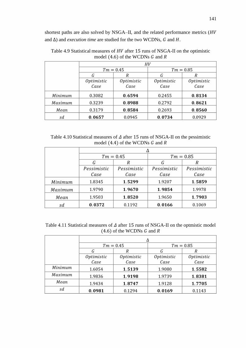
141

shortest paths are also solved by NSGA–II, and the related performance metrics (𝐻𝑉

and Δ) and execution time are studied for the two WCDNs, 𝐺 and 𝐻.

Table 4.9 Statistical measures of 𝐻𝑉 after 15 runs of NSGA-II on the optimistic


𝐻𝑉

𝑇𝑚 = 0.45 𝑇𝑚 = 0.85

𝐺 𝑅 𝐺 𝑅

𝑂𝑝𝑡𝑖𝑚𝑖𝑠𝑡𝑖𝑐

𝐶𝑎𝑠𝑒 𝑂𝑝𝑡𝑖𝑚𝑖𝑠𝑡𝑖𝑐

𝐶𝑎𝑠𝑒


𝐶𝑎𝑠𝑒


𝐶𝑎𝑠𝑒

𝑀𝑖𝑛𝑖𝑚𝑢𝑚 0.3082 𝟎. 𝟔𝟓𝟗𝟒 0.2455 𝟎. 𝟖𝟏𝟑𝟒

𝑀𝑎𝑥𝑖𝑚𝑢𝑚 0.3239 𝟎. 𝟖𝟗𝟖𝟖 0.2792 𝟎. 𝟖𝟔𝟐𝟏

𝑀𝑒𝑎𝑛 0.3179 𝟎. 𝟖𝟓𝟖𝟒 0.2693 𝟎. 𝟖𝟓𝟔𝟎

𝑠𝑑 𝟎. 𝟎𝟔𝟓𝟕 0.0945 𝟎. 𝟎𝟕𝟑𝟒 0.0929

Table 4.10 Statistical measures of 𝛥 after 15 runs of NSGA-II on the pessimistic


Δ

𝑇𝑚 = 0.45 𝑇𝑚 = 0.85

𝐺 𝑅 𝐺 𝑅


𝐶𝑎𝑠𝑒 𝑃𝑒𝑠𝑠𝑖𝑚𝑖𝑠𝑡𝑖𝑐

𝐶𝑎𝑠𝑒


𝐶𝑎𝑠𝑒


𝐶𝑎𝑠𝑒

𝑀𝑖𝑛𝑖𝑚𝑢𝑚 1.8345 𝟏. 𝟓𝟐𝟗𝟗 1.9207 𝟏. 𝟓𝟖𝟓𝟗

𝑀𝑎𝑥𝑖𝑚𝑢𝑚 1.9790 𝟏. 𝟗𝟔𝟕𝟎 𝟏. 𝟗𝟖𝟓𝟒 1.9978

𝑀𝑒𝑎𝑛 1.9503 𝟏. 𝟖𝟓𝟐𝟎 1.9650 𝟏. 𝟕𝟗𝟎𝟑

𝑠𝑑 𝟎. 𝟎𝟑𝟕𝟐 0.1192 𝟎. 𝟎𝟏𝟔𝟔 0.1069

Table 4.11 Statistical measures of 𝛥 after 15 runs of NSGA-II on the optmistic model

(4.6) of the WCDNs 𝐺 and 𝑅

Δ

𝑇𝑚 = 0.45 𝑇𝑚 = 0.85

𝐺 𝑅 𝐺 𝑅



𝐶𝑎𝑠𝑒


𝐶𝑎𝑠𝑒


𝐶𝑎𝑠𝑒

𝑀𝑖𝑛𝑖𝑚𝑢𝑚 1.6054 𝟏. 𝟓𝟏𝟑𝟗 1.9080 𝟏. 𝟓𝟓𝟖𝟐 𝑀𝑎𝑥𝑖𝑚𝑢𝑚 1.9836 𝟏. 𝟗𝟏𝟗𝟖 1.9739 𝟏. 𝟖𝟑𝟖𝟏 𝑀𝑒𝑎𝑛 1.9434 𝟏. 𝟖𝟕𝟒𝟕 1.9128 𝟏. 𝟕𝟕𝟎𝟓 𝑠𝑑 𝟎. 𝟎𝟗𝟖𝟏 0.1294 𝟎. 𝟎𝟏𝟔𝟗 0.1143

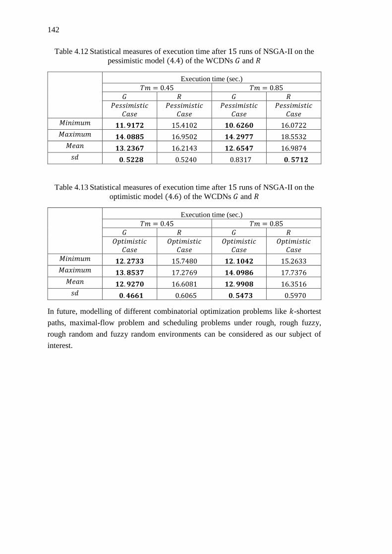
142


pessimistic model (4.4) of the WCDNs 𝐺 and 𝑅

Execution time (sec.)

𝑇𝑚 = 0.45 𝑇𝑚 = 0.85

𝐺 𝑅 𝐺 𝑅





𝐶𝑎𝑠𝑒

𝑀𝑖𝑛𝑖𝑚𝑢𝑚 𝟏𝟏. 𝟗𝟏𝟕𝟐 15.4102 𝟏𝟎. 𝟔𝟐𝟔𝟎 16.0722 𝑀𝑎𝑥𝑖𝑚𝑢𝑚 𝟏𝟒. 𝟎𝟖𝟖𝟓 16.9502 𝟏𝟒. 𝟐𝟗𝟕𝟕 18.5532 𝑀𝑒𝑎𝑛 𝟏𝟑. 𝟐𝟑𝟔𝟕 16.2143 𝟏𝟐. 𝟔𝟓𝟒𝟕 16.9874 𝑠𝑑 𝟎. 𝟓𝟐𝟐𝟖 0.5240 0.8317 𝟎. 𝟓𝟕𝟏𝟐


optimistic model (4.6) of the WCDNs 𝐺 and 𝑅

Execution time (sec.)

𝑇𝑚 = 0.45 𝑇𝑚 = 0.85

𝐺 𝑅 𝐺 𝑅



𝐶𝑎𝑠𝑒



𝐶𝑎𝑠𝑒

𝑀𝑖𝑛𝑖𝑚𝑢𝑚 𝟏𝟐. 𝟐𝟕𝟑𝟑 15.7480 𝟏𝟐. 𝟏𝟎𝟒𝟐 15.2633 𝑀𝑎𝑥𝑖𝑚𝑢𝑚 𝟏𝟑. 𝟖𝟓𝟑𝟕 17.2769 𝟏𝟒. 𝟎𝟗𝟖𝟔 17.7376 𝑀𝑒𝑎𝑛 𝟏𝟐. 𝟗𝟐𝟕𝟎 16.6081 𝟏𝟐. 𝟗𝟗𝟎𝟖 16.3516 𝑠𝑑 𝟎. 𝟒𝟔𝟔𝟏 0.6065 𝟎. 𝟓𝟒𝟕𝟑 0.5970

In future, modelling of different combinatorial optimization problems like 𝑘-shortest

paths, maximal-flow problem and scheduling problems under rough, rough fuzzy,

rough random and fuzzy random environments can be considered as our subject of

interest.

143

Chapter 5

Uncertain Multi-objective Multi-item

Fixed Charge Solid Transportation

Problem with Budget Constraint

User

Text Box

144

User

Text Box

145

Chapter 5

Uncertain Multi-objective Multi-item Fixed

Charged Solid Transportation with Budget

Constraint

5.1 Introduction

The notion of classical transportation problem (TP) is to determine an optimal solution

(transportation plan) such that the transportation cost is minimized. The noteworthy

work of F.L. Hitchcock (1941) introduced the term transportation problem, by

modelling it as a conventional optimization problem with two-dimensional properties,

i.e., supply and demand. However, apart from supply and demand constraints, in real-

world scenarios, often we need to consider the mode of transportation (e.g., goods train,

cargo flights and trucks), types of goods, etc. Under such circumstances, a TP is

extended to a solid transportation problem (STP), where apart from source and

destination constraints, an additional constraint, related to the modes of transportation

(convenience) or types of goods is considered. E.D. Schell (1955), first extended the

classical TP to solid transportation problem. Later, Bhatia et al. (1976) minimized the

shipping time of an STP. Afterwards, Jiménez and Verdegay (1998), in their work, dealt

with an STP and solved the problem by considering the supply quantities, demand

quantities and conveyance capacities as interval values instead of point values.

Hirsch and Dantzig (1968) presented another variant of TP, called fixed charge

transportation problem (FTP). In FTP, the objective is to determine an optimal

transportation plan that minimizes the overall cost between sources and destinations.

The overall cost has two components: variable shipping cost and an independent fixed

charge. The shipping cost depends directly on the quantity of the transported item(s)

from sources to destinations whereas, the fixed charge, which commonly appears due

to the expenditure related to permit fees, property tax or toll charges, etc., is associated

with every feasible transportation plan. Several researchers (Kennington and Unger

1976; Sun et al. 1998; Adlakha and Kowalski 2003) have proposed different solution

approaches for FTP.

Most of the real-life decision making problems, can be well expressed with multiple

conflicting criteria and are usually formulated as multi-objective optimization

problems. Moreover, the associated parameters for such problems may be imprecise

User

Text Box

146

due to insufficient or inexact information owing to incompleteness or lack of evidence,

statistical analysis, etc. Therefore, to process and represent imprecise or ill-defined

data for decision making problems, many researchers have presented a number of

improved theories, e.g., fuzzy set (L.A. Zadeh 1965), type-2 fuzzy set (L.A. Zadeh

1975a, b), rough set (Z. Pawlak 1982), etc. Likewise, the uncertainty theory proposed

by B. Liu (2007) deals with the belief degrees of human being, which can appropriately

evaluate personal belief degree of experts in terms of uncertain measure.

In the literature, there are many studies done in the field of TP with uncertain input

parameters. Kaur and Kumar (2012) described a new solution technique for TP by

considering the transportation costs as generalized trapezoidal fuzzy numbers. In the

multi-objective domain, Bit et al. (1993) solved the multi-objective STP using

Zimmermann’s fuzzy programming technique (H.-J. Zimmermann 1978). Later, Gen

et al. (1995) proposed a bi-objective STP with fuzzy parameters. Recently, Kundu et

al. (2017a) used interval type-2 fuzzy multi-criteria group decision making approach to

solve a transportation mode selection problem. Considering the budget limitation of a

TP, Kundu et al. (2013b) discussed a multi-objective STP by imposing budget

constraints at destinations with fuzzy random hybrid parameters. Later, Baidya and

Bera (2014) proposed a budget constraint STP by representing transportation cost,

availability and demand, and conveyance capacity as interval numbers. Besides, Kundu

et al. (2014b) also investigated a fuzzy multi-criteria decision making (MCDM)

approach to determine the most preferred transportation mode, to solve an STP.

Recently, Das et al. (2017) solved the green STP under type-2 fuzzy environment.

Considering fixed charge TP in imprecise domain, Liu et al. (2008) presented an FTP

in a fuzzy environment and solved it by genetic algorithm. Later, Pramanik et al.

(2015b) revisited the FTP by considering the shipping cost, fixed charge, availability

and demand in a two-stage supply chain under type-2 Gaussian fuzzy transportation

network.

Uncertainty theory, founded by B. Liu (2007) and refined by B. Liu (2009, 2010), is a

branch of axiomatic mathematics for modelling human uncertainty. Nowadays,

uncertainty theory has been applied to many areas such as economics (Yang and Gao

2016; Yang and Gao 2017), management (Gao and Yao 2015; Gao et al. 2017) and

finance (Chen and Gao 2013; Guo and Gao 2017). Similarly, under the framework of

uncertainty theory, different variants of TP are also studied in the literature (Sheng and

Yao 2012a, 2012b; Cui and Sheng 2013; Mou et al. 2013; Guo et al. 2015; Chen et al.

2017). In Table 5.1, we have furnished some recent reviews of different variants of TP

under diverse uncertain environments.

In spite of all the developments of TP, there are several gaps in the literature which are

listed below.

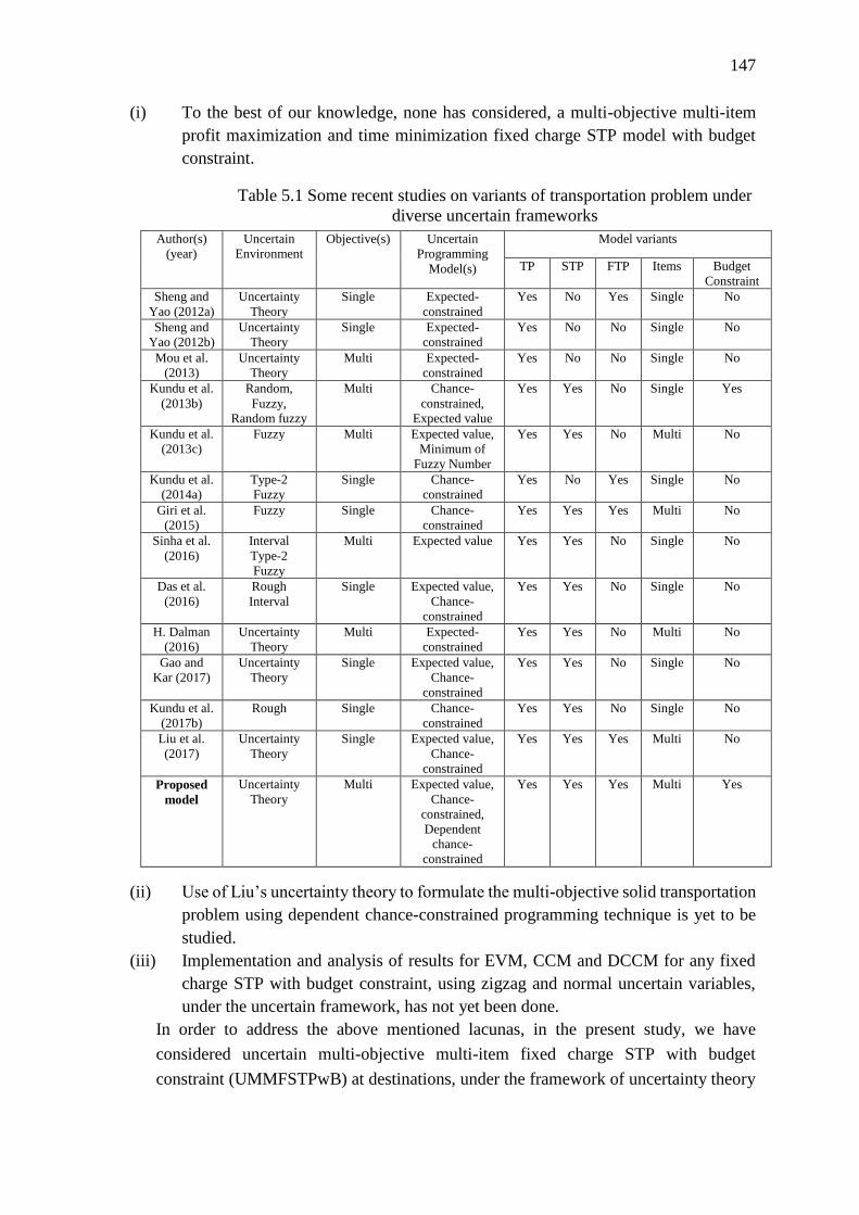
147

(i) To the best of our knowledge, none has considered, a multi-objective multi-item

profit maximization and time minimization fixed charge STP model with budget

constraint.

Table 5.1 Some recent studies on variants of transportation problem under

diverse uncertain frameworks

(ii) Use of Liu’s uncertainty theory to formulate the multi-objective solid transportation

problem using dependent chance-constrained programming technique is yet to be

studied.

(iii) Implementation and analysis of results for EVM, CCM and DCCM for any fixed

charge STP with budget constraint, using zigzag and normal uncertain variables,

under the uncertain framework, has not yet been done.

In order to address the above mentioned lacunas, in the present study, we have

considered uncertain multi-objective multi-item fixed charge STP with budget

constraint (UMMFSTPwB) at destinations, under the framework of uncertainty theory

Author(s)

(year)

Uncertain

Environment

Objective(s) Uncertain

Programming

Model(s)

Model variants

TP STP FTP Items Budget

Constraint

Sheng and

Yao (2012a)

Uncertainty

Theory

Single Expected-

constrained

Yes No Yes Single No

Sheng and

Yao (2012b)

Uncertainty

Theory

Single Expected-

constrained

Yes No No Single No

Mou et al.

(2013)

Uncertainty

Theory

Multi Expected-

constrained

Yes No No Single No

Kundu et al.

(2013b)

Random,

Fuzzy,

Random fuzzy

Multi Chance-

constrained,

Expected value

Yes Yes No Single Yes

Kundu et al.

(2013c)

Fuzzy Multi Expected value,

Minimum of

Fuzzy Number

Yes Yes No Multi No

Kundu et al.

(2014a)

Type-2

Fuzzy

Single Chance-

constrained

Yes No Yes Single No

Giri et al.

(2015)

Fuzzy Single Chance-

constrained

Yes Yes Yes Multi No

Sinha et al.

(2016)

Interval

Type-2

Fuzzy

Multi Expected value Yes Yes No Single No

Das et al.

(2016)

Rough

Interval

Single Expected value,

Chance-

constrained

Yes Yes No Single No

H. Dalman

(2016)

Uncertainty

Theory

Multi Expected-

constrained

Yes Yes No Multi No

Gao and

Kar (2017)

Uncertainty

Theory


Chance-

constrained


Kundu et al.

(2017b)

Rough Single Chance-

constrained


Liu et al.

(2017)

Uncertainty

Theory


Chance-

constrained

Yes Yes Yes Multi No

Proposed

model

Uncertainty

Theory

Multi Expected value,

Chance-

constrained,

Dependent

chance-

constrained

Yes Yes Yes Multi Yes

148

(B. Liu 2007). The problem is formulated in three different models: expected value

model (EVM), chance-constrained model (CCM) and dependent chance-constrained

model (DCCM). Consecutively, each model is solved by three different multi-objective

compromise techniques: linear weighted method, global criterion method and fuzzy

programming method.

The subsequent sections of this chapter are organized as follow. The uncertain

programming models, EVM, CCM and DCCM of the proposed UMMFSTPwB are

presented in Section 5.2. The crisp equivalent for each of the models of UMMFSTPwB

is formulated in Section 5.3. Some related theorems of the three different compromise

multi-objective solution methodologies are explained in Section 5.4. In Section 5.5, we

present the numerical examples to illustrate the model, and the results are discussed

with comparative analysis. Finally, the epilogue of our study is presented in Section

5.6.

5.2 Problem Definition

A solid transportation problem is concerned with transportation of homogeneous

products from source 𝑖 to destination 𝑗 via conveyance 𝑘 (≥ 2) (trucks, cargo van,

goods train, etc.) for which we need to find an optimal transportation plan so that the

total transportation cost is minimized. A balanced condition in STP assumes that the

total supply at source depots, total demand at destinations and total conveyance

capacities are equal. But, in reality, we may encounter the following situations in the

context of TP. They are mentioned as follow.

(i) Adequate quantities of the item at the sources to satisfy the demands at

destinations.

(ii) The conveyances should have the ability to suffice the demand at destinations.

(iii) There may be a requirement of multiple items or products at destinations for

which we may need to consider shipment of heterogeneous items from source 𝑖 to

destination 𝑗 via conveyance 𝑘.

(iv) Limited budget at destinations.

(v) Besides transportation cost, fixed charge cost can also exist when a

transportation activity is initiated from source 𝑖 to destination 𝑗.

(vi) In some situations, often we require to optimize several objectives at the same

time which are conflicting in nature. In the context of transportation problem, these

objectives may be the minimization of total transportation cost, total delivery time,

deterioration of breakable goods, maximization of profit, etc.

In order to consider some of the practical situations mentioned above, in our study, we

have presented a profit maximization and time minimization of multi-item fixed charge

solid transportation problem with budget constraint. The following notations are used

to formulate a multi-objective multi-item fixed charge solid transportation problem

with budget constraint (MMFSTPwB) model.

149

𝑚 : Number of origins/source depots.

𝑛 : Number of destinations/demand points.

𝐾 : Number of conveyances utilize for transportation of products.

𝑟 : Number of different types of items to be transported.

For 𝑖 = 1, 2, … ,𝑚, 𝑗 = 1, 2, … , 𝑛, 𝑘 = 1, 2, … , 𝐾 and 𝑝 = 1, 2, … , 𝑟

𝑎𝑖𝑝

: Amount of item 𝑝 available at source 𝑖.

𝑏𝑗𝑝

: Demand of item 𝑝 at destination 𝑗.

𝑒𝑘: Transportation capacity of conveyance 𝑘.

𝑐𝑖𝑗𝑘𝑝

: Cost for transporting one unit of item 𝑝 from source 𝑖 to destination 𝑗

by conveyance 𝑘.

𝑓𝑖𝑗𝑘𝑝

: Fixed charge with respect to the transportation activity for transporting

item 𝑝 from source 𝑖 to destination 𝑗 by conveyance 𝑘.

𝑥𝑖𝑗𝑘𝑝

: Quantity of item 𝑝 transported from source 𝑖 to destination 𝑗 by

conveyance 𝑘.

𝑡𝑖𝑗𝑘𝑝

: Time required for transporting item 𝑝 with respect to transportation

activity from source 𝑖 to destination 𝑗 by conveyance 𝑘.

𝑠𝑗𝑝

: Selling price per unit of item 𝑝 at the destination 𝑗.

𝑣𝑖𝑝

: Purchasing cost per unit of item 𝑝 at the source 𝑖.

𝐵𝑗: Budget at destination 𝑗.

To initiate a transportation activity from source 𝑖 to destination 𝑗 we need to reserve

conveyance 𝑘, leading to a fixed charge. In other words, a fixed charge will be added

to the direct transportation cost, if 𝑥𝑖𝑗𝑘𝑝 > 0. Therefore, in our problem, the fixed charge

is incorporated using a binary decision variable 𝑦𝑖𝑗𝑘𝑝

, where 𝑦𝑖𝑗𝑘𝑝 =

{1 ; 𝑖𝑓 𝑥𝑖𝑗𝑘

𝑝 > 0

0 ; 𝑜𝑡ℎ𝑒𝑟𝑤𝑖𝑠𝑒 ∀ 𝑝, 𝑖, 𝑗, 𝑘. Accordingly, we present the mathematical model of

MMFSTPwB in (5.1).

In model (5.1), the first objective is to maximize the overall profit earned after

transporting all the required items from each source to every destination points through

the available conveyances. The second objective minimizes the total transportation time

for shipment of all the required items from all sources to all destinations. The

significance of the constraints of the model (5.1) is discussed below.

The first constraint determines that the total quantity of item 𝑝 which is shipped from

source 𝑖 does not exceed the availability 𝑎𝑖𝑝. The second constraint determines the

shipment of a total quantity of item 𝑝 at destination 𝑗, satisfies at least the demand 𝑏𝑗𝑝.

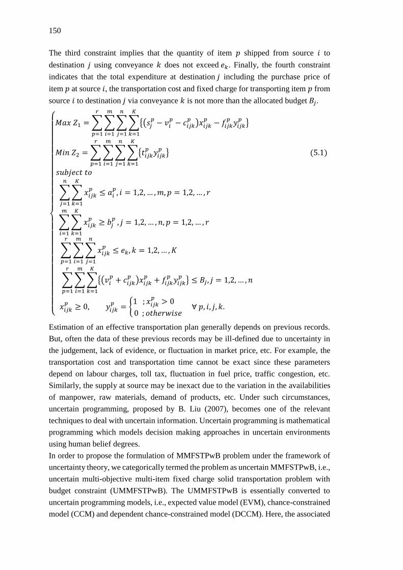
150

The third constraint implies that the quantity of item 𝑝 shipped from source 𝑖 to

destination 𝑗 using conveyance 𝑘 does not exceed 𝑒𝑘. Finally, the fourth constraint

indicates that the total expenditure at destination 𝑗 including the purchase price of

item 𝑝 at source 𝑖, the transportation cost and fixed charge for transporting item 𝑝 from

source 𝑖 to destination 𝑗 via conveyance 𝑘 is not more than the allocated budget 𝐵𝑗.

{

𝑀𝑎𝑥 𝑍1 =∑∑∑∑{(𝑠𝑗

𝑝 − 𝑣𝑖𝑝 − 𝑐𝑖𝑗𝑘

𝑝 )𝑥𝑖𝑗𝑘𝑝 − 𝑓𝑖𝑗𝑘

𝑝 𝑦𝑖𝑗𝑘𝑝 }

𝐾

𝑘=1

𝑛

𝑗=1

𝑚

𝑖=1

𝑟

𝑝=1

𝑀𝑖𝑛 𝑍2 =∑∑∑∑{𝑡𝑖𝑗𝑘𝑝 𝑦𝑖𝑗𝑘

𝑝 }

𝐾

𝑘=1

𝑛

𝑗=1

𝑚

𝑖=1

𝑟

𝑝=1

(5.1)


∑∑𝑥𝑖𝑗𝑘𝑝

𝐾

𝑘=1

𝑛

𝑗=1

≤ 𝑎𝑖𝑝, 𝑖 = 1,2, … ,𝑚, 𝑝 = 1,2, … , 𝑟

∑∑𝑥𝑖𝑗𝑘𝑝 ≥ 𝑏𝑗

𝑝

𝐾

𝑘=1

𝑚

𝑖=1

, 𝑗 = 1,2, … , 𝑛, 𝑝 = 1,2, … , 𝑟

∑∑∑𝑥𝑖𝑗𝑘𝑝

𝑛

𝑗=1

𝑚

𝑖=1

𝑟

𝑝=1

≤ 𝑒𝑘, 𝑘 = 1,2, … , 𝐾

∑∑∑{(𝑣𝑖𝑝 + 𝑐𝑖𝑗𝑘

𝑝 )𝑥𝑖𝑗𝑘𝑝 + 𝑓𝑖𝑗𝑘

𝑝 𝑦𝑖𝑗𝑘𝑝 }

𝐾

𝑘=1

𝑚

𝑖=1

𝑟

𝑝=1

≤ 𝐵𝑗 , 𝑗 = 1,2, … , 𝑛

𝑥𝑖𝑗𝑘𝑝 ≥ 0, 𝑦𝑖𝑗𝑘

𝑝 = {1 ; 𝑥𝑖𝑗𝑘

𝑝 > 0

0 ; 𝑜𝑡ℎ𝑒𝑟𝑤𝑖𝑠𝑒 ∀ 𝑝, 𝑖, 𝑗, 𝑘.

Estimation of an effective transportation plan generally depends on previous records.

But, often the data of these previous records may be ill-defined due to uncertainty in

the judgement, lack of evidence, or fluctuation in market price, etc. For example, the

transportation cost and transportation time cannot be exact since these parameters

depend on labour charges, toll tax, fluctuation in fuel price, traffic congestion, etc.

Similarly, the supply at source may be inexact due to the variation in the availabilities

of manpower, raw materials, demand of products, etc. Under such circumstances,

uncertain programming, proposed by B. Liu (2007), becomes one of the relevant

techniques to deal with uncertain information. Uncertain programming is mathematical

programming which models decision making approaches in uncertain environments

using human belief degrees.

In order to propose the formulation of MMFSTPwB problem under the framework of

uncertainty theory, we categorically termed the problem as uncertain MMFSTPwB, i.e.,

uncertain multi-objective multi-item fixed charge solid transportation problem with

budget constraint (UMMFSTPwB). The UMMFSTPwB is essentially converted to

uncertain programming models, i.e., expected value model (EVM), chance-constrained

model (CCM) and dependent chance-constrained model (DCCM). Here, the associated

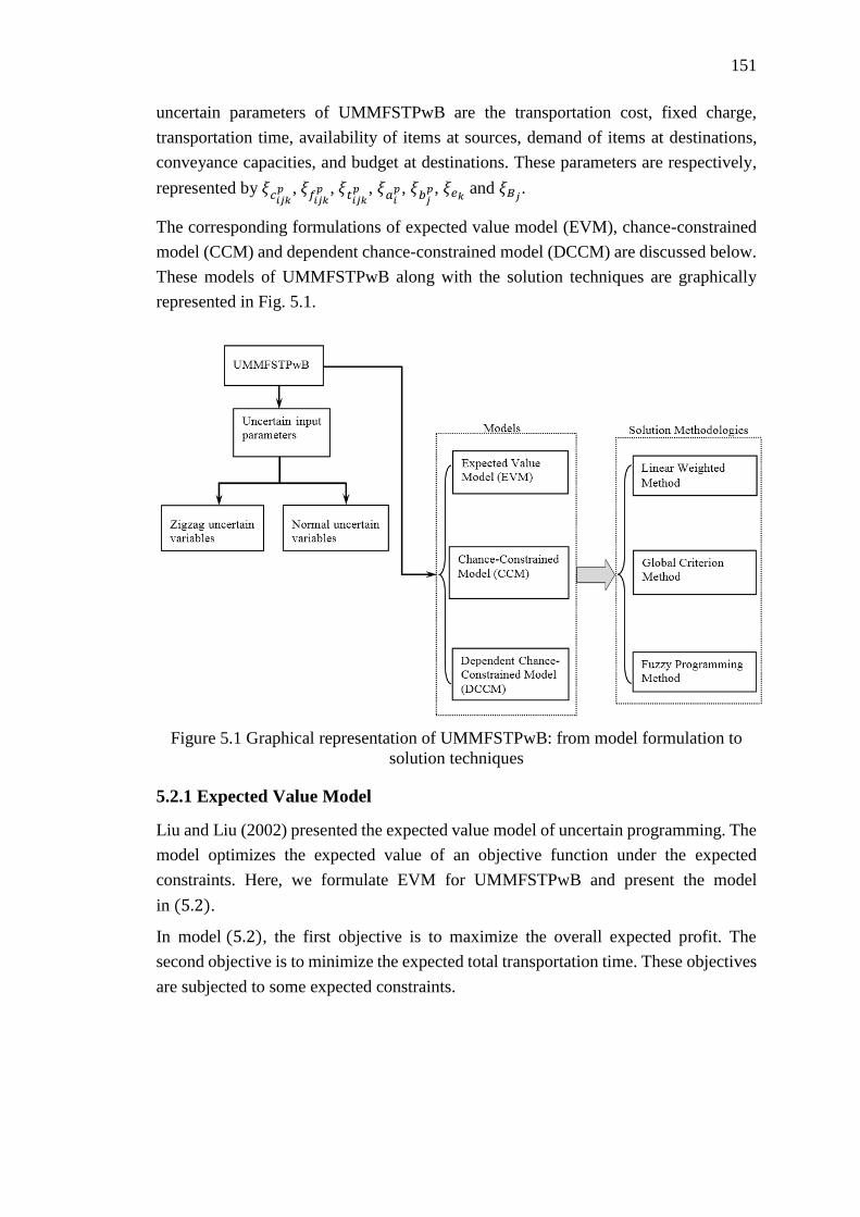
151

uncertain parameters of UMMFSTPwB are the transportation cost, fixed charge,

transportation time, availability of items at sources, demand of items at destinations,

conveyance capacities, and budget at destinations. These parameters are respectively,

represented by 𝜉𝑐𝑖𝑗𝑘𝑝 , 𝜉𝑓𝑖𝑗𝑘

𝑝 , 𝜉𝑡𝑖𝑗𝑘𝑝 , 𝜉𝑎𝑖

𝑝, 𝜉𝑏𝑗𝑝, 𝜉𝑒𝑘 and 𝜉𝐵𝑗 .

The corresponding formulations of expected value model (EVM), chance-constrained

model (CCM) and dependent chance-constrained model (DCCM) are discussed below.

These models of UMMFSTPwB along with the solution techniques are graphically

represented in Fig. 5.1.

Figure 5.1 Graphical representation of UMMFSTPwB: from model formulation to

solution techniques

5.2.1 Expected Value Model

Liu and Liu (2002) presented the expected value model of uncertain programming. The

model optimizes the expected value of an objective function under the expected

constraints. Here, we formulate EVM for UMMFSTPwB and present the model

in (5.2).

In model (5.2), the first objective is to maximize the overall expected profit. The

second objective is to minimize the expected total transportation time. These objectives

are subjected to some expected constraints.

152

{

𝑀𝑎𝑥 𝐸[𝑍1] = 𝐸 [∑ ∑ ∑ ∑ {(𝑠𝑗

𝑝 − 𝑣𝑖𝑝 − 𝜉𝑐𝑖𝑗𝑘

𝑝 ) 𝑥𝑖𝑗𝑘𝑝 − 𝜉𝑓𝑖𝑗𝑘

𝑝 𝑦𝑖𝑗𝑘𝑝 }𝐾

𝑘=1𝑛𝑗=1

𝑚𝑖=1

𝑟𝑝=1 ]

𝑀𝑖𝑛 𝐸[𝑍2] = 𝐸 [∑ ∑ ∑ ∑ 𝜉𝑡𝑖𝑗𝑘𝑝 𝑦𝑖𝑗𝑘

𝑝𝐾𝑘=1

𝑛𝑗=1

𝑚𝑖=1

𝑟𝑝=1 ]

𝑠𝑢𝑏𝑗𝑒𝑐𝑡 𝑡𝑜 (5.2)

𝐸 [∑ ∑ 𝑥𝑖𝑗𝑘𝑝 − 𝜉𝑎𝑖

𝑝𝐾𝑘=1

𝑛𝑗=1 ] ≤ 0, 𝑖 = 1,2, … ,𝑚, 𝑝 = 1,2, … , 𝑟

𝐸 [∑ ∑ 𝑥𝑖𝑗𝑘𝑝 − 𝜉𝑏𝑗

𝑝𝐾𝑘=1

𝑚𝑖=1 ] ≥ 0, 𝑗 = 1,2, … , 𝑛, 𝑝 = 1,2, … , 𝑟

𝐸[∑ ∑ ∑ 𝑥𝑖𝑗𝑘𝑝𝑛

𝑗=1 − 𝜉𝑒𝑘𝑚𝑖=1

𝑟𝑝=1 ] ≤ 0, 𝑘 = 1,2, … , 𝐾

𝐸 [∑ ∑ ∑ {(𝑣𝑖𝑝 + 𝜉𝑐𝑖𝑗𝑘

𝑝 ) 𝑥𝑖𝑗𝑘𝑝 + 𝜉𝑓𝑖𝑗𝑘


𝑘=1𝑚𝑖=1

𝑟𝑝=1 − 𝜉𝐵𝑗] ≤ 0, 𝑗 = 1,2, … , 𝑛


𝑝 = {1 ; 𝑖𝑓 𝑥𝑖𝑗𝑘

𝑝 > 0


5.2.2 Chance-constrained Model

Chance-constrained programming is an alternate method to deal with optimization of a

problem under uncertain environment. The basic idea of CCM (Charnes and Cooper

1959; B. Liu 2002) is that it allows violation of constraints, but we need to ensure that

the constraints should hold at some chance level (confidence level). Here, we develop

the chance-constrained model for UMMFSTPwB and present it in (5.3).

{

𝑀𝑎𝑥 ��1

𝑀𝑖𝑛 ��2 𝑠𝑢𝑏𝑗𝑒𝑐𝑡 𝑡𝑜 (5.3)

ℳ {∑ ∑ ∑ ∑ [(𝑠𝑗𝑝 − 𝑣𝑖

𝑝 − 𝜉𝑐𝑖𝑗𝑘𝑝 ) 𝑥𝑖𝑗𝑘

𝑝 − 𝜉𝑓𝑖𝑗𝑘𝑝 𝑦𝑖𝑗𝑘

𝑝 ]𝐾𝑘=1

𝑛𝑗=1

𝑚𝑖=1

𝑟𝑝=1 ≥ ��1} ≥ α1

ℳ {∑ ∑ ∑ ∑ [𝜉𝑡𝑖𝑗𝑘𝑝 𝑦𝑖𝑗𝑘

𝑝 ]𝐾𝑘=1

𝑛𝑗=1

𝑚𝑖=1

𝑟𝑝=1 ≤ ��2} ≥ α2

ℳ {∑ ∑ 𝑥𝑖𝑗𝑘𝑝 − 𝜉𝑎𝑖

𝑝𝐾𝑘=1

𝑛𝑗=1 ≤ 0} ≥ 𝛽𝑖

𝑝, 𝑖 = 1,2, … ,𝑚, 𝑝 = 1,2, … , 𝑟

ℳ {∑ ∑ 𝑥𝑖𝑗𝑘𝑝 − 𝜉𝑏𝑗

𝑝𝐾𝑘=1

𝑛𝑖=1 ≥ 0} ≥ 𝛾𝑗

𝑝, 𝑗 = 1,2, … , 𝑛, 𝑝 = 1,2, … , 𝑟

ℳ{∑ ∑ ∑ 𝑥𝑖𝑗𝑘𝑝𝑛


𝑟𝑝=1 ≤ 0} ≥ 𝛿𝑘, 𝑘 = 1,2, … , 𝐾

ℳ {∑ ∑ ∑ {(𝑣𝑖𝑝 + 𝜉𝑐𝑖𝑗𝑘

𝑝 ) 𝑥𝑖𝑗𝑘𝑝 + 𝜉𝑓𝑖𝑗𝑘


𝑘=1𝑚𝑖=1

𝑟𝑝=1 − 𝜉𝐵𝑗 ≤ 0} ≥ 𝜌𝑗 , 𝑗 = 1,2, … , 𝑛



𝑝 > 0


In CCM, 𝛼1, 𝛼2, 𝛽𝑖𝑝 , 𝛾𝑗

𝑝, 𝛿𝑘 and 𝜌𝑗 are predetermined confidence levels. The objectives

��1 and ��2 determine the critical values corresponding to the first and second constraints.

The first constraint determines the 𝛼1-optimistic value of the overall profit

corresponding to an 𝛼1-transportation plan and the second constraint determines the

α2-pessimistic value of the shipping/transportation time with respect to an 𝛼2-

transportation plan. Moreover, the remaining constraints (third to sixth) of model (5.3),

also hold at their corresponding chance levels, which are at least 𝛽𝑖𝑝, 𝛾𝑗

𝑝, 𝛿𝑘 and 𝜌𝑗.

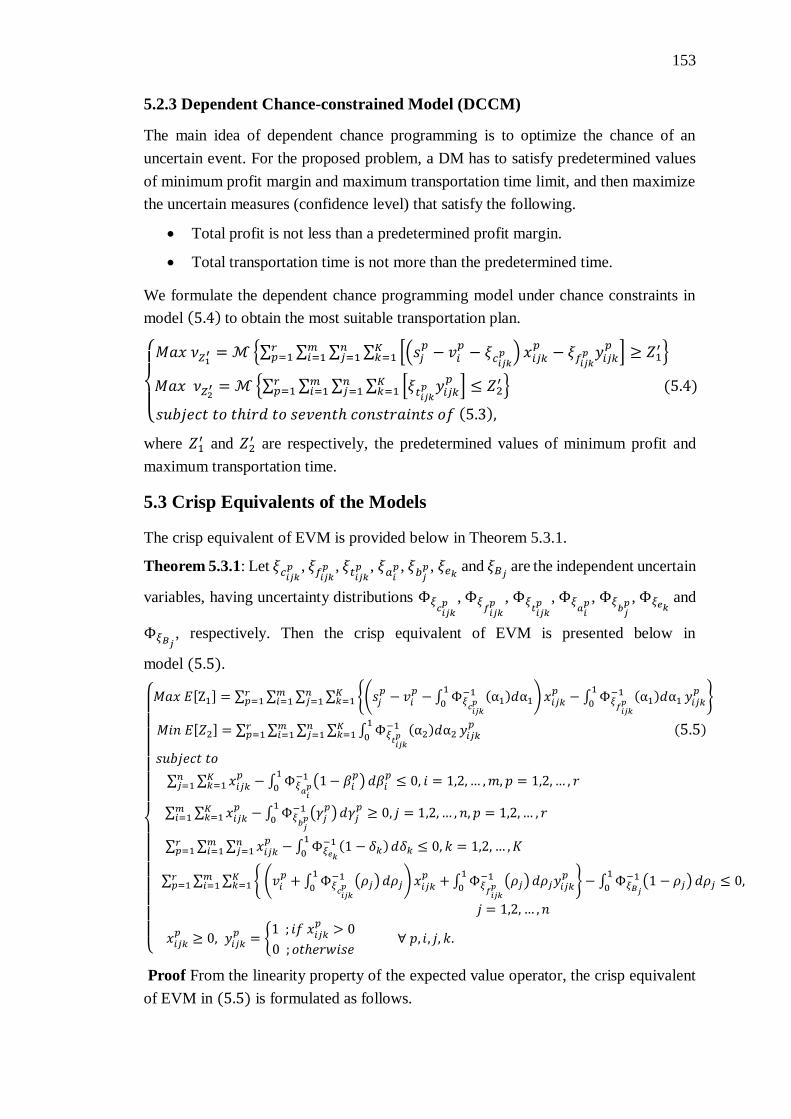
153

5.2.3 Dependent Chance-constrained Model (DCCM)

The main idea of dependent chance programming is to optimize the chance of an

uncertain event. For the proposed problem, a DM has to satisfy predetermined values

of minimum profit margin and maximum transportation time limit, and then maximize

the uncertain measures (confidence level) that satisfy the following.

Total profit is not less than a predetermined profit margin.

Total transportation time is not more than the predetermined time.

We formulate the dependent chance programming model under chance constraints in

model (5.4) to obtain the most suitable transportation plan.

{

𝑀𝑎𝑥 𝜈𝑍1′ =ℳ {∑ ∑ ∑ ∑ [(𝑠𝑗

𝑝− 𝑣𝑖

𝑝− 𝜉𝑐𝑖𝑗𝑘

𝑝 ) 𝑥𝑖𝑗𝑘𝑝− 𝜉𝑓𝑖𝑗𝑘

𝑝 𝑦𝑖𝑗𝑘𝑝 ]𝐾

𝑘=1𝑛𝑗=1

𝑚𝑖=1

𝑟𝑝=1 ≥ 𝑍1

′}

𝑀𝑎𝑥 𝜈𝑍2′ =ℳ {∑ ∑ ∑ ∑ [𝜉𝑡𝑖𝑗𝑘𝑝 𝑦𝑖𝑗𝑘

𝑝 ]𝐾𝑘=1

𝑛𝑗=1

𝑚𝑖=1

𝑟𝑝=1 ≤ 𝑍2

′ } (5.4)

𝑠𝑢𝑏𝑗𝑒𝑐𝑡 𝑡𝑜 𝑡ℎ𝑖𝑟𝑑 𝑡𝑜 𝑠𝑒𝑣𝑒𝑛𝑡ℎ 𝑐𝑜𝑛𝑠𝑡𝑟𝑎𝑖𝑛𝑡𝑠 𝑜𝑓 (5.3),

where 𝑍1′ and 𝑍2

′ are respectively, the predetermined values of minimum profit and

maximum transportation time.

5.3 Crisp Equivalents of the Models

The crisp equivalent of EVM is provided below in Theorem 5.3.1.

Theorem 5.3.1: Let 𝜉𝑐𝑖𝑗𝑘𝑝 , 𝜉𝑓𝑖𝑗𝑘


𝑝 , 𝜉𝑏𝑗𝑝 , 𝜉𝑒𝑘 and 𝜉𝐵𝑗 are the independent uncertain

variables, having uncertainty distributions Φ𝜉𝑐𝑖𝑗𝑘𝑝 , Φ𝜉

𝑓𝑖𝑗𝑘𝑝 , Φ𝜉

𝑡𝑖𝑗𝑘𝑝 , Φ𝜉

𝑎𝑖𝑝 , Φ𝜉

𝑏𝑗𝑝 , Φ𝜉𝑒𝑘

and

Φ𝜉𝐵𝑗, respectively. Then the crisp equivalent of EVM is presented below in

model (5.5).

{

𝑀𝑎𝑥 𝐸[Z1] = ∑ ∑ ∑ ∑ {(𝑠𝑗

𝑝 − 𝑣𝑖𝑝 − ∫ Φ𝜉


−1 (α1)𝑑α11

0)𝑥𝑖𝑗𝑘

𝑝 − ∫ Φ𝜉𝑓𝑖𝑗𝑘𝑝

−1 (α1)𝑑α11

0𝑦𝑖𝑗𝑘𝑝 }𝐾

𝑘=1𝑛𝑗=1

𝑚𝑖=1

𝑟𝑝=1

𝑀𝑖𝑛 𝐸[𝑍2] = ∑ ∑ ∑ ∑ ∫ Φ𝜉𝑡𝑖𝑗𝑘𝑝

−1 (α2)𝑑α21

0𝑦𝑖𝑗𝑘𝑝𝐾

𝑘=1𝑛𝑗=1

𝑚𝑖=1

𝑟𝑝=1 (5.5)


∑ ∑ 𝑥𝑖𝑗𝑘𝑝 − ∫ Φ𝜉

𝑎𝑖𝑝

−1 (1− 𝛽𝑖𝑝)

1

0𝑑𝛽𝑖

𝑝𝐾𝑘=1

𝑛𝑗=1 ≤ 0, 𝑖 = 1,2,… ,𝑚, 𝑝 = 1,2,… , 𝑟

∑ ∑ 𝑥𝑖𝑗𝑘𝑝 − ∫ Φ𝜉

𝑏𝑗𝑝

−1 (𝛾𝑗𝑝)

1

0𝑑𝛾𝑗

𝑝𝐾𝑘=1

𝑚𝑖=1 ≥ 0, 𝑗 = 1,2,… , 𝑛, 𝑝 = 1,2,… , 𝑟

∑ ∑ ∑ 𝑥𝑖𝑗𝑘𝑝𝑛

𝑗=1 − ∫ Φ𝜉𝑒𝑘

−1 (1 − 𝛿𝑘)1

0𝑑𝛿𝑘

𝑚𝑖=1

𝑟𝑝=1 ≤ 0, 𝑘 = 1,2, … ,𝐾

∑ ∑ ∑ { (𝑣𝑖𝑝 + ∫ Φ𝜉


−1 (𝜌𝑗)1

0𝑑𝜌𝑗)𝑥𝑖𝑗𝑘

𝑝 + ∫ Φ𝜉𝑓𝑖𝑗𝑘𝑝

−1 (𝜌𝑗)1

0𝑑𝜌𝑗𝑦𝑖𝑗𝑘

𝑝 }𝐾𝑘=1

𝑚𝑖=1

𝑟𝑝=1 − ∫ Φ𝜉𝐵𝑗

−1 (1 − 𝜌𝑗)1

0𝑑𝜌𝑗 ≤ 0,

𝑗 = 1,2, … , 𝑛



𝑝 > 0


Proof From the linearity property of the expected value operator, the crisp equivalent

of EVM in (5.5) is formulated as follows.

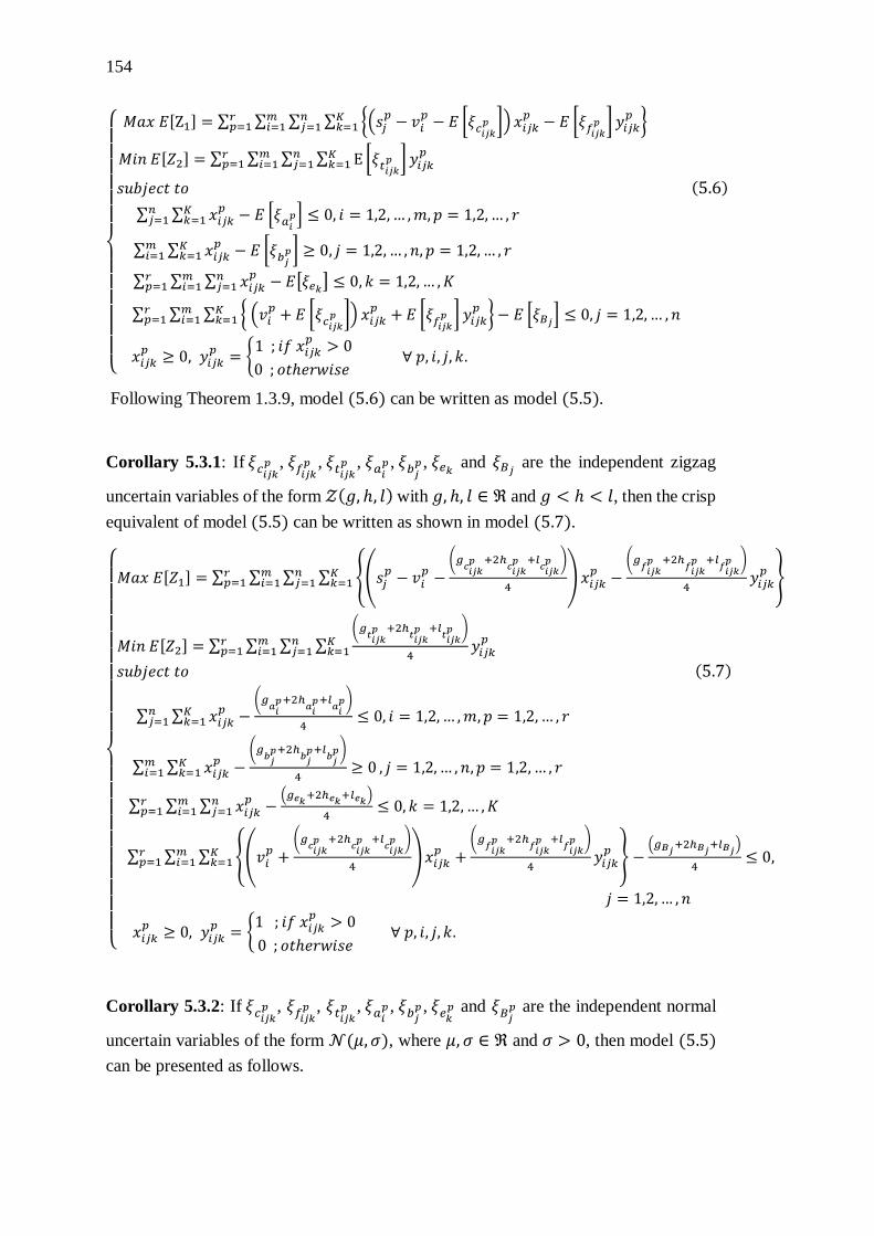
154

{

𝑀𝑎𝑥 𝐸[Z1] = ∑ ∑ ∑ ∑ {(𝑠𝑗

𝑝− 𝑣𝑖

𝑝− 𝐸 [𝜉𝑐𝑖𝑗𝑘

𝑝 ]) 𝑥𝑖𝑗𝑘𝑝− 𝐸 [𝜉𝑓𝑖𝑗𝑘

𝑝 ] 𝑦𝑖𝑗𝑘𝑝 } 𝐾

𝑘=1𝑛𝑗=1

𝑚𝑖=1

𝑟𝑝=1

𝑀𝑖𝑛 𝐸[𝑍2] = ∑ ∑ ∑ ∑ E [𝜉𝑡𝑖𝑗𝑘𝑝 ] 𝑦𝑖𝑗𝑘

𝑝𝐾𝑘=1

𝑛𝑗=1

𝑚𝑖=1

𝑟𝑝=1


∑ ∑ 𝑥𝑖𝑗𝑘𝑝− 𝐸 [𝜉𝑎𝑖

𝑝]𝐾𝑘=1

𝑛𝑗=1 ≤ 0, 𝑖 = 1,2, … ,𝑚, 𝑝 = 1,2, … , 𝑟

∑ ∑ 𝑥𝑖𝑗𝑘𝑝− 𝐸 [𝜉𝑏𝑗

𝑝]𝐾𝑘=1

𝑚𝑖=1 ≥ 0, 𝑗 = 1,2, … , 𝑛, 𝑝 = 1,2, … , 𝑟


𝑗=1 − 𝐸[𝜉𝑒𝑘]𝑚𝑖=1

𝑟𝑝=1 ≤ 0, 𝑘 = 1,2, … , 𝐾

∑ ∑ ∑ { (𝑣𝑖𝑝+ 𝐸 [𝜉𝑐𝑖𝑗𝑘

𝑝 ]) 𝑥𝑖𝑗𝑘𝑝+ 𝐸 [𝜉𝑓𝑖𝑗𝑘

𝑝 ] 𝑦𝑖𝑗𝑘𝑝 }𝐾

𝑘=1𝑚𝑖=1

𝑟𝑝=1 − 𝐸 [𝜉𝐵𝑗] ≤ 0, 𝑗 = 1,2, … , 𝑛

𝑥𝑖𝑗𝑘𝑝≥ 0, 𝑦𝑖𝑗𝑘

𝑝= {

1 ; 𝑖𝑓 𝑥𝑖𝑗𝑘𝑝> 0


Following Theorem 1.3.9, model (5.6) can be written as model (5.5).

Corollary 5.3.1: If 𝜉𝑐𝑖𝑗𝑘𝑝 , 𝜉𝑓𝑖𝑗𝑘


𝑝 , 𝜉𝑏𝑗𝑝 , 𝜉𝑒𝑘 and 𝜉𝐵𝑗 are the independent zigzag

uncertain variables of the form 𝒵(𝑔, ℎ, 𝑙) with 𝑔, ℎ, 𝑙 ∈ ℜ and 𝑔 < ℎ < 𝑙, then the crisp

equivalent of model (5.5) can be written as shown in model (5.7).

{

𝑀𝑎𝑥 𝐸[𝑍1] = ∑ ∑ ∑ ∑ {(𝑠𝑗

𝑝− 𝑣𝑖

𝑝−(𝑔

𝑐𝑖𝑗𝑘𝑝 +2ℎ

𝑐𝑖𝑗𝑘𝑝 +𝑙

𝑐𝑖𝑗𝑘𝑝 )

4)𝑥𝑖𝑗𝑘

𝑝−(𝑔

𝑓𝑖𝑗𝑘𝑝 +2ℎ

𝑓𝑖𝑗𝑘𝑝 +𝑙

𝑓𝑖𝑗𝑘𝑝 )


𝑘=1𝑛𝑗=1

𝑚𝑖=1

𝑟𝑝=1

𝑀𝑖𝑛 𝐸[𝑍2] = ∑ ∑ ∑ ∑(𝑔

𝑡𝑖𝑗𝑘𝑝 +2ℎ

𝑡𝑖𝑗𝑘𝑝 +𝑙

𝑡𝑖𝑗𝑘𝑝 )

4𝑦𝑖𝑗𝑘𝑝𝐾

𝑘=1𝑛𝑗=1

𝑚𝑖=1

𝑟𝑝=1


∑ ∑ 𝑥𝑖𝑗𝑘𝑝−(𝑔

𝑎𝑖𝑝+2ℎ

𝑎𝑖𝑝+𝑙

𝑎𝑖𝑝)

4𝐾𝑘=1

𝑛𝑗=1 ≤ 0, 𝑖 = 1,2, … ,𝑚, 𝑝 = 1,2, … , 𝑟

∑ ∑ 𝑥𝑖𝑗𝑘𝑝 −

(𝑔𝑏𝑗𝑝+2ℎ

𝑏𝑗𝑝+𝑙

𝑏𝑗𝑝)

4≥ 0𝐾

𝑘=1𝑚𝑖=1 , 𝑗 = 1,2, … , 𝑛, 𝑝 = 1,2, … , 𝑟


𝑗=1 −(𝑔𝑒𝑘+2ℎ𝑒𝑘+𝑙𝑒𝑘)

4

𝑚𝑖=1

𝑟𝑝=1 ≤ 0, 𝑘 = 1,2, … , 𝐾

∑ ∑ ∑ {(𝑣𝑖𝑝 +

(𝑔𝑐𝑖𝑗𝑘𝑝 +2ℎ

𝑐𝑖𝑗𝑘𝑝 +𝑙

𝑐𝑖𝑗𝑘𝑝 )

4)𝑥𝑖𝑗𝑘

𝑝 +(𝑔

𝑓𝑖𝑗𝑘𝑝 +2ℎ

𝑓𝑖𝑗𝑘𝑝 +𝑙

𝑓𝑖𝑗𝑘𝑝 )


𝑘=1𝑚𝑖=1

𝑟𝑝=1 −

(𝑔𝐵𝑗+2ℎ𝐵𝑗+𝑙𝐵𝑗)

4≤ 0,

𝑗 = 1,2, … , 𝑛



𝑝 > 0


Corollary 5.3.2: If 𝜉𝑐𝑖𝑗𝑘𝑝 , 𝜉𝑓𝑖𝑗𝑘


𝑝 , 𝜉𝑏𝑗𝑝 , 𝜉𝑒𝑘

𝑝 and 𝜉𝐵𝑗𝑝 are the independent normal

uncertain variables of the form 𝒩(𝜇, 𝜎), where 𝜇, 𝜎 ∈ ℜ and 𝜎 > 0, then model (5.5)

can be presented as follows.

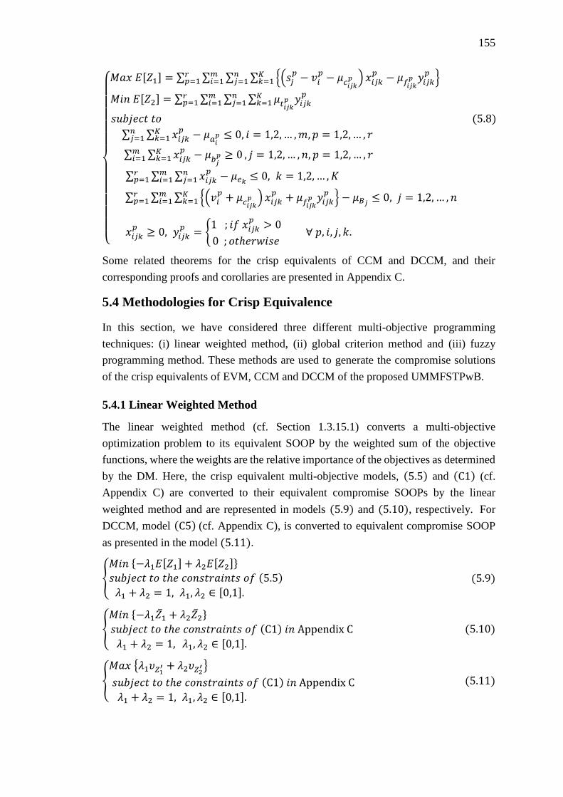
155

{

𝑀𝑎𝑥 𝐸[𝑍1] = ∑ ∑ ∑ ∑ {(𝑠𝑗

𝑝 − 𝑣𝑖𝑝 − 𝜇𝑐𝑖𝑗𝑘

𝑝 ) 𝑥𝑖𝑗𝑘𝑝 − 𝜇𝑓𝑖𝑗𝑘


𝑘=1𝑛𝑗=1

𝑚𝑖=1

𝑟𝑝=1

𝑀𝑖𝑛 𝐸[𝑍2] = ∑ ∑ ∑ ∑ 𝜇𝑡𝑖𝑗𝑘𝑝 𝑦𝑖𝑗𝑘

𝑝𝐾𝑘=1

𝑛𝑗=1

𝑚𝑖=1

𝑟𝑝=1


∑ ∑ 𝑥𝑖𝑗𝑘𝑝 − 𝜇𝑎𝑖

𝑝𝐾𝑘=1

𝑛𝑗=1 ≤ 0, 𝑖 = 1,2, … ,𝑚, 𝑝 = 1,2, … , 𝑟

∑ ∑ 𝑥𝑖𝑗𝑘𝑝 − 𝜇𝑏𝑗

𝑝 ≥ 0𝐾𝑘=1

𝑚𝑖=1 , 𝑗 = 1,2, … , 𝑛, 𝑝 = 1,2, … , 𝑟


𝑗=1 − 𝜇𝑒𝑘𝑚𝑖=1

𝑟𝑝=1 ≤ 0, 𝑘 = 1,2, … , 𝐾

∑ ∑ ∑ {(𝑣𝑖𝑝 + 𝜇𝑐𝑖𝑗𝑘

𝑝 ) 𝑥𝑖𝑗𝑘𝑝 + 𝜇𝑓𝑖𝑗𝑘


𝑘=1𝑚𝑖=1

𝑟𝑝=1 − 𝜇𝐵𝑗 ≤ 0, 𝑗 = 1,2, … , 𝑛



𝑝 > 0


Some related theorems for the crisp equivalents of CCM and DCCM, and their

corresponding proofs and corollaries are presented in Appendix C.

5.4 Methodologies for Crisp Equivalence

In this section, we have considered three different multi-objective programming

techniques: (i) linear weighted method, (ii) global criterion method and (iii) fuzzy

programming method. These methods are used to generate the compromise solutions

of the crisp equivalents of EVM, CCM and DCCM of the proposed UMMFSTPwB.

5.4.1 Linear Weighted Method

The linear weighted method (cf. Section 1.3.15.1) converts a multi-objective

optimization problem to its equivalent SOOP by the weighted sum of the objective

functions, where the weights are the relative importance of the objectives as determined

by the DM. Here, the crisp equivalent multi-objective models, (5.5) and (C1) (cf.

Appendix C) are converted to their equivalent compromise SOOPs by the linear

weighted method and are represented in models (5.9) and (5.10), respectively. For

DCCM, model (C5) (cf. Appendix C), is converted to equivalent compromise SOOP

as presented in the model (5.11).

{

𝑀𝑖𝑛 {−𝜆1𝐸[𝑍1] + 𝜆2𝐸[𝑍2]}

𝑠𝑢𝑏𝑗𝑒𝑐𝑡 𝑡𝑜 𝑡ℎ𝑒 𝑐𝑜𝑛𝑠𝑡𝑟𝑎𝑖𝑛𝑡𝑠 𝑜𝑓 (5.5)

𝜆1 + 𝜆2 = 1, 𝜆1, 𝜆2 ∈ [0,1].

(5.9)

{

𝑀𝑖𝑛 {−𝜆1��1 + 𝜆2��2}

𝑠𝑢𝑏𝑗𝑒𝑐𝑡 𝑡𝑜 𝑡ℎ𝑒 𝑐𝑜𝑛𝑠𝑡𝑟𝑎𝑖𝑛𝑡𝑠 𝑜𝑓 (C1) 𝑖𝑛 Appendix C

𝜆1 + 𝜆2 = 1, 𝜆1, 𝜆2 ∈ [0,1].

(5.10)

{

𝑀𝑎𝑥 {𝜆1𝜐𝑍1′ + 𝜆2𝜐𝑍2′}

𝑠𝑢𝑏𝑗𝑒𝑐𝑡 𝑡𝑜 𝑡ℎ𝑒 𝑐𝑜𝑛𝑠𝑡𝑟𝑎𝑖𝑛𝑡𝑠 𝑜𝑓 (C1) 𝑖𝑛 Appendix C

𝜆1 + 𝜆2 = 1, 𝜆1, 𝜆2 ∈ [0,1].

(5.11)

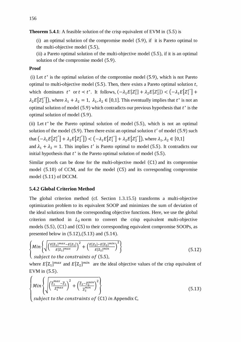
156

Theorem 5.4.1: A feasible solution of the crisp equivalent of EVM in (5.5) is

(i) an optimal solution of the compromise model (5.9), if it is Pareto optimal to

the multi-objective model (5.5),

(ii) a Pareto optimal solution of the multi-objective model (5.5), if it is an optimal

solution of the compromise model (5.9).

Proof

(i) Let 𝑡∗ is the optimal solution of the compromise model (5.9), which is not Pareto

optimal to multi-objective model (5.5). Then, there exists a Pareto optimal solution 𝑡,

which dominates 𝑡∗ or 𝑡 ≺ 𝑡∗. It follows, (−𝜆1𝐸[𝑍1𝑡] + 𝜆2𝐸[𝑍2

𝑡]) < (−𝜆1𝐸[𝑍1𝑡∗] +

𝜆2𝐸[𝑍2𝑡∗]), where 𝜆1 + 𝜆2 = 1, 𝜆1, 𝜆2 ∈ [0,1]. This eventually implies that 𝑡∗ is not an

optimal solution of model (5.9) which contradicts our previous hypothesis that 𝑡∗ is the

optimal solution of model (5.9).

(ii) Let 𝑡∗ be the Pareto optimal solution of model (5.5), which is not an optimal

solution of the model (5.9). Then there exist an optimal solution 𝑡′ of model (5.9) such

that (−𝜆1𝐸[𝑍1𝑡′] + 𝜆2𝐸[𝑍2

𝑡′]) < (−𝜆1𝐸[𝑍1𝑡∗] + 𝜆2𝐸[𝑍2

𝑡∗]), where 𝜆1, 𝜆2 ∈ [0,1]

and 𝜆1 + 𝜆2 = 1. This implies 𝑡′ is Pareto optimal to model (5.5). It contradicts our

initial hypothesis that 𝑡∗ is the Pareto optimal solution of model (5.5).

Similar proofs can be done for the multi-objective model (C1) and its compromise

model (5.10) of CCM, and for the model (C5) and its corresponding compromise

model (5.11) of DCCM.

5.4.2 Global Criterion Method

The global criterion method (cf. Section 1.3.15.5) transforms a multi-objective

optimization problem to its equivalent SOOP and minimizes the sum of deviation of

the ideal solutions from the corresponding objective functions. Here, we use the global

criterion method in 𝐿2 norm to convert the crisp equivalent multi-objective

models (5.5), (C1) and (C5) to their corresponding equivalent compromise SOOPs, as

presented below in (5.12),(5.13) and (5.14).

{𝑀𝑖𝑛 {√(

𝐸[Z1]𝑚𝑎𝑥−𝐸[𝑍1]

𝐸[Z1]𝑚𝑎𝑥 )

2

+ (𝐸[𝑍2]−𝐸[Z2]

𝑚𝑖𝑛

𝐸[Z2]𝑚𝑖𝑛 )

2

}

𝑠𝑢𝑏𝑗𝑒𝑐𝑡 𝑡𝑜 𝑡ℎ𝑒 𝑐𝑜𝑛𝑠𝑡𝑟𝑎𝑖𝑛𝑡𝑠 𝑜𝑓 (5.5),

(5.12)

where 𝐸[Z1]𝑚𝑎𝑥 and 𝐸[Z2]

𝑚𝑖𝑛 are the ideal objective values of the crisp equivalent of

EVM in (5.5).

{

𝑀𝑖𝑛{√(

𝑍1𝑚𝑎𝑥

−𝑍1

𝑍1𝑚𝑎𝑥 )

2

+ (𝑍2−𝑍2

𝑚𝑖𝑛

𝑍2𝑚𝑖𝑛 )

2

}

𝑠𝑢𝑏𝑗𝑒𝑐𝑡 𝑡𝑜 𝑡ℎ𝑒 𝑐𝑜𝑛𝑠𝑡𝑟𝑎𝑖𝑛𝑡𝑠 𝑜𝑓 (C1) 𝑖𝑛 Appendix C,

(5.13)

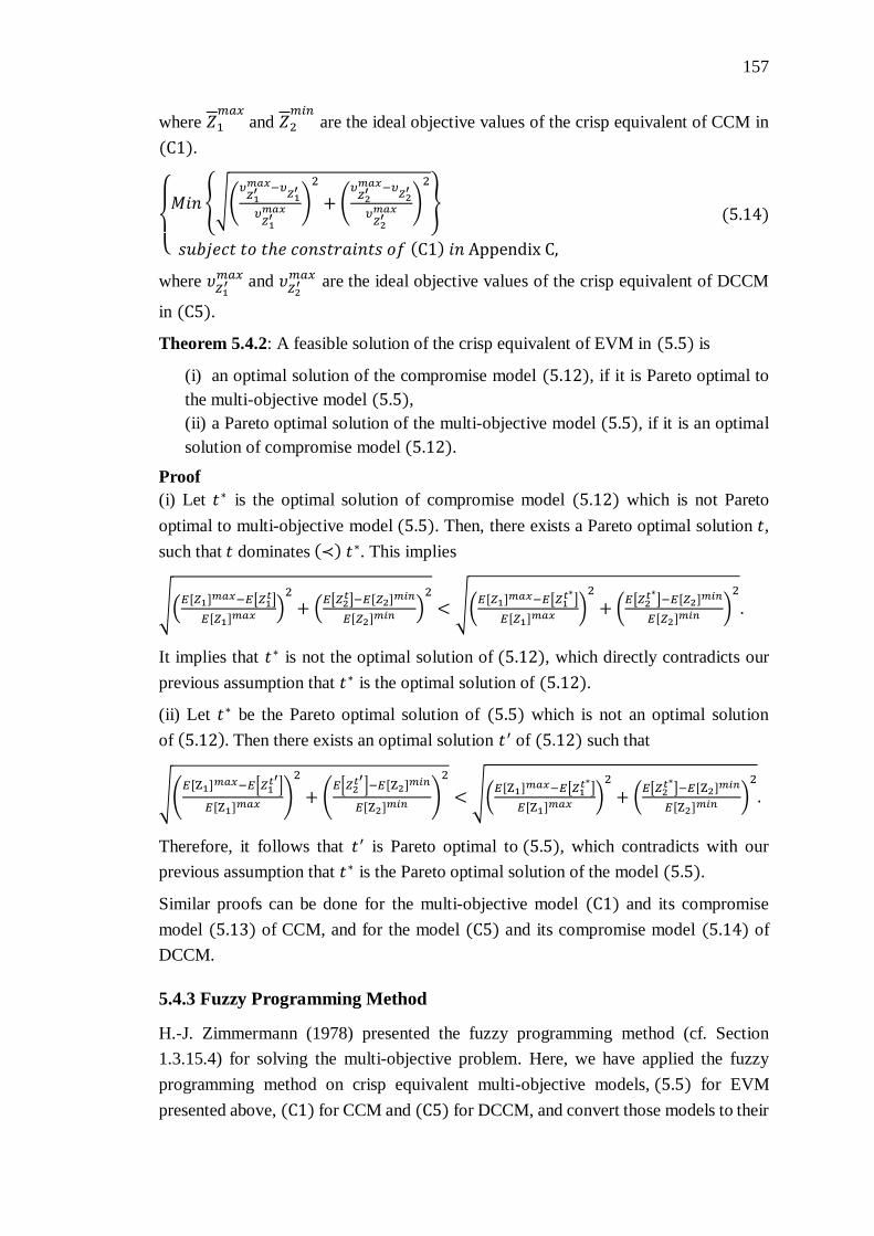
157

where 𝑍1𝑚𝑎𝑥

and 𝑍2𝑚𝑖𝑛

are the ideal objective values of the crisp equivalent of CCM in

(C1).

{

𝑀𝑖𝑛 {√(

𝜐𝑍1′𝑚𝑎𝑥−𝜐

𝑍1′

𝜐𝑍1′𝑚𝑎𝑥 )

2

+ (𝜐𝑍2′𝑚𝑎𝑥−𝜐

𝑍2′

𝜐𝑍2′

𝑚𝑎𝑥 )

2

}

𝑠𝑢𝑏𝑗𝑒𝑐𝑡 𝑡𝑜 𝑡ℎ𝑒 𝑐𝑜𝑛𝑠𝑡𝑟𝑎𝑖𝑛𝑡𝑠 𝑜𝑓 (C1) 𝑖𝑛 Appendix C,

(5.14)

where 𝜐𝑍1′𝑚𝑎𝑥 and 𝜐𝑍2′

𝑚𝑎𝑥 are the ideal objective values of the crisp equivalent of DCCM

in (C5).


(i) an optimal solution of the compromise model (5.12), if it is Pareto optimal to

the multi-objective model (5.5),

(ii) a Pareto optimal solution of the multi-objective model (5.5), if it is an optimal

solution of compromise model (5.12).

Proof

(i) Let 𝑡∗ is the optimal solution of compromise model (5.12) which is not Pareto


such that 𝑡 dominates (≺) 𝑡∗. This implies

√(𝐸[𝑍1]

𝑚𝑎𝑥−𝐸[𝑍1𝑡]

𝐸[𝑍1]𝑚𝑎𝑥 )

2

+ (𝐸[𝑍2

𝑡]−𝐸[𝑍2]𝑚𝑖𝑛

𝐸[𝑍2]𝑚𝑖𝑛 )

2

< √(𝐸[𝑍1]

𝑚𝑎𝑥−𝐸[𝑍1𝑡∗]

𝐸[𝑍1]𝑚𝑎𝑥 )

2

+ (𝐸[𝑍2

𝑡∗]−𝐸[𝑍2]𝑚𝑖𝑛

𝐸[𝑍2]𝑚𝑖𝑛 )

2

.

It implies that 𝑡∗ is not the optimal solution of (5.12), which directly contradicts our

previous assumption that 𝑡∗ is the optimal solution of (5.12).

(ii) Let 𝑡∗ be the Pareto optimal solution of (5.5) which is not an optimal solution

of (5.12). Then there exists an optimal solution 𝑡′ of (5.12) such that

√(𝐸[Z1]

𝑚𝑎𝑥−𝐸[𝑍1𝑡′]


2

+ (𝐸[𝑍2

𝑡′]−𝐸[Z2]𝑚𝑖𝑛


2

< √(𝐸[Z1]

𝑚𝑎𝑥−𝐸[𝑍1𝑡∗]


2

+ (𝐸[𝑍2

𝑡∗]−𝐸[Z2]𝑚𝑖𝑛


2

.

Therefore, it follows that 𝑡′ is Pareto optimal to (5.5), which contradicts with our

previous assumption that 𝑡∗ is the Pareto optimal solution of the model (5.5).


model (5.13) of CCM, and for the model (C5) and its compromise model (5.14) of

DCCM.

5.4.3 Fuzzy Programming Method

H.-J. Zimmermann (1978) presented the fuzzy programming method (cf. Section

1.3.15.4) for solving the multi-objective problem. Here, we have applied the fuzzy

programming method on crisp equivalent multi-objective models, (5.5) for EVM

presented above, (C1) for CCM and (C5) for DCCM, and convert those models to their

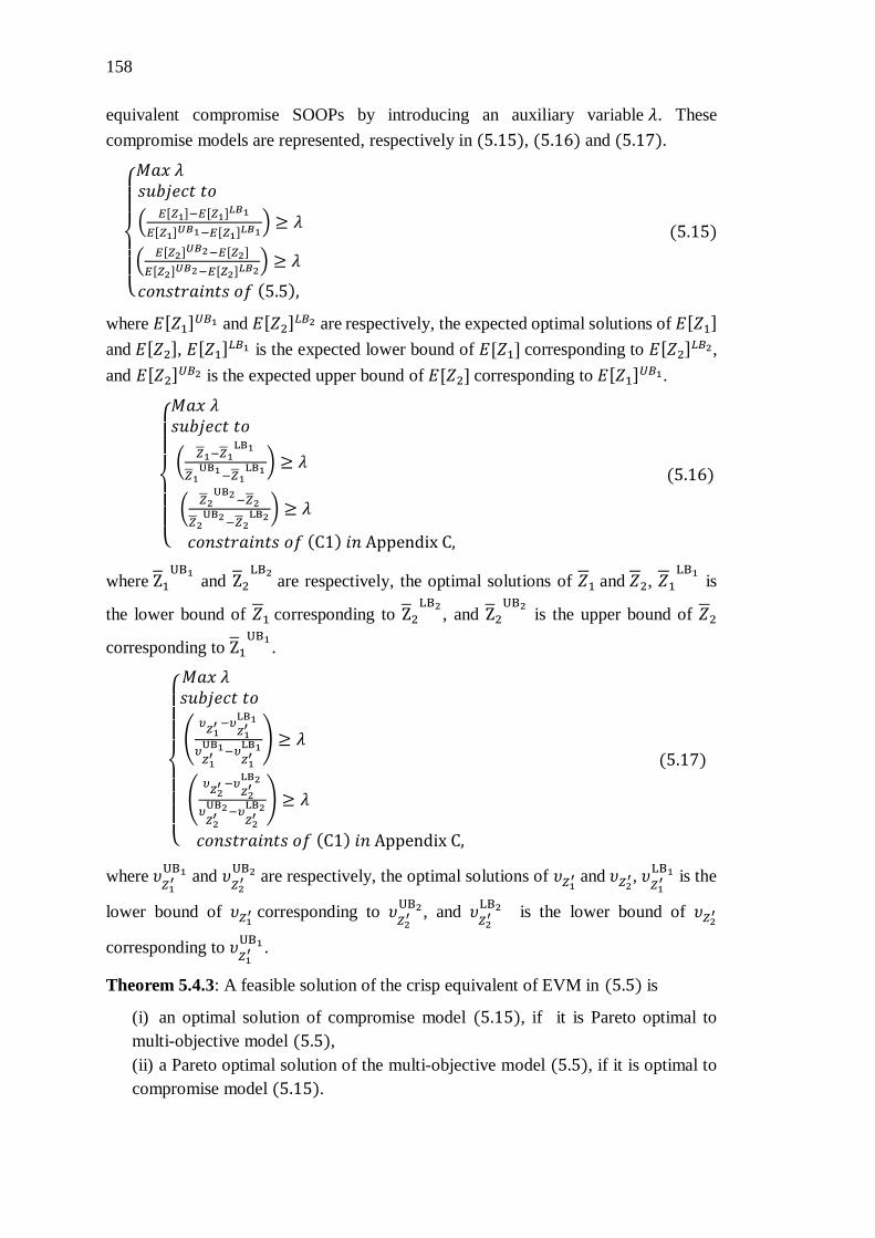
158

equivalent compromise SOOPs by introducing an auxiliary variable 𝜆. These

compromise models are represented, respectively in (5.15), (5.16) and (5.17).

{


(𝐸[𝑍1]−𝐸[𝑍1]

𝐿𝐵1

𝐸[𝑍1]𝑈𝐵1−𝐸[𝑍1]

𝐿𝐵1) ≥ 𝜆

(𝐸[𝑍2]

𝑈𝐵2−𝐸[𝑍2]


𝐿𝐵2) ≥ 𝜆


(5.15)

where 𝐸[𝑍1]𝑈𝐵1 and 𝐸[𝑍2]

𝐿𝐵2 are respectively, the expected optimal solutions of 𝐸[𝑍1]

and 𝐸[𝑍2], 𝐸[𝑍1]𝐿𝐵1 is the expected lower bound of 𝐸[𝑍1] corresponding to 𝐸[𝑍2]

𝐿𝐵2,

and 𝐸[𝑍2]𝑈𝐵2 is the expected upper bound of 𝐸[𝑍2] corresponding to 𝐸[𝑍1]

𝑈𝐵1.

{


(𝑍1−𝑍1

LB1

𝑍1UB1−𝑍1

LB1) ≥ 𝜆

(𝑍2

UB2−𝑍2

𝑍2UB2−𝑍2

LB2) ≥ 𝜆

𝑐𝑜𝑛𝑠𝑡𝑟𝑎𝑖𝑛𝑡𝑠 𝑜𝑓 (C1) 𝑖𝑛 Appendix C,

(5.16)

where Z1UB1

and Z2LB2 are respectively, the optimal solutions of 𝑍1 and 𝑍2, 𝑍1

LB1 is

the lower bound of 𝑍1 corresponding to Z2LB2

, and Z2UB2

is the upper bound of 𝑍2

corresponding to Z1UB1

.

{


(𝜐𝑍1′ −𝜐

𝑍1′

LB1

𝜐𝑍1′UB1−𝜐

𝑍1′LB1) ≥ 𝜆

(𝜐𝑍2′ −𝜐

𝑍2′

LB2

𝜐𝑍2′UB2−𝜐

𝑍2′LB2) ≥ 𝜆

𝑐𝑜𝑛𝑠𝑡𝑟𝑎𝑖𝑛𝑡𝑠 𝑜𝑓 (C1) 𝑖𝑛 Appendix C,

(5.17)

where 𝜐𝑍1′UB1 and 𝜐

𝑍2′UB2 are respectively, the optimal solutions of 𝜐𝑍1′ and 𝜐𝑍2′, 𝜐𝑍1′

LB1 is the

lower bound of 𝜐𝑍1′ corresponding to 𝜐𝑍2′UB2 , and 𝜐

𝑍2′LB2 is the lower bound of 𝜐𝑍2′

corresponding to 𝜐𝑍1′UB1 .


(i) an optimal solution of compromise model (5.15), if it is Pareto optimal to

multi-objective model (5.5),

(ii) a Pareto optimal solution of the multi-objective model (5.5), if it is optimal to

compromise model (5.15).

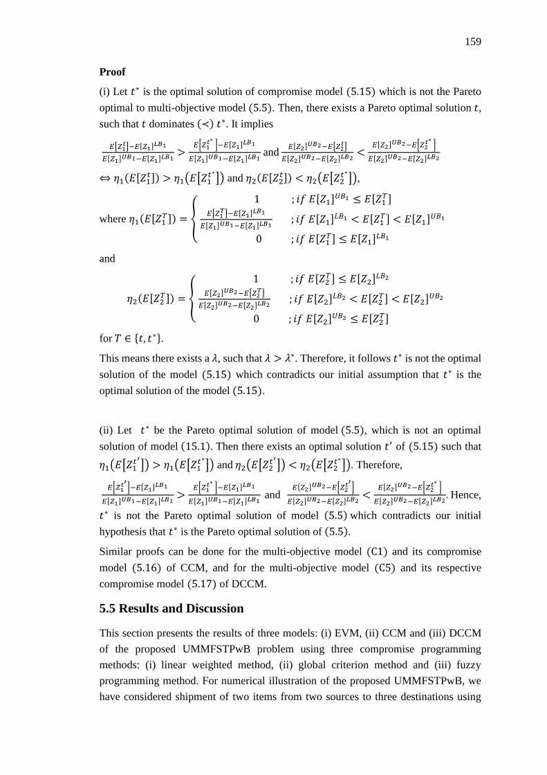
159

Proof

(i) Let 𝑡∗ is the optimal solution of compromise model (5.15) which is not the Pareto


such that 𝑡 dominates (≺) 𝑡∗. It implies

𝐸[𝑍1

𝑡]−𝐸[𝑍1]𝐿𝐵1

𝐸[𝑍1]𝑈𝐵1−𝐸[𝑍1]𝐿𝐵1>

𝐸[𝑍1𝑡∗ ]−𝐸[𝑍1]

𝐿𝐵1

𝐸[𝑍1]𝑈𝐵1−𝐸[𝑍1]𝐿𝐵1 and

𝐸[𝑍2]𝑈𝐵2−𝐸[𝑍2

𝑡]


𝐿𝐵2<


𝑡∗ ]


𝐿𝐵2

⇔ 휂1(𝐸[𝑍1𝑡]) > 휂1(𝐸[𝑍1

𝑡∗]) and 휂2(𝐸[𝑍2𝑡]) < 휂2(𝐸[𝑍2

𝑡∗]),

where 휂1(𝐸[𝑍1𝑇]) = {

1 ; 𝑖𝑓 𝐸[𝑍1]𝑈𝐵1 ≤ 𝐸[𝑍1

𝑇]𝐸[𝑍1

𝑇]−𝐸[𝑍1]𝐿𝐵1

𝐸[𝑍1]𝑈𝐵1−𝐸[𝑍1]𝐿𝐵1 ; 𝑖𝑓 𝐸[𝑍1]

𝐿𝐵1 < 𝐸[𝑍1𝑇] < 𝐸[𝑍1]

𝑈𝐵1

0 ; 𝑖𝑓 𝐸[𝑍1𝑇] ≤ 𝐸[𝑍1]

𝐿𝐵1

and

휂2(𝐸[𝑍2𝑇]) = {

1 ; 𝑖𝑓 𝐸[𝑍2𝑇] ≤ 𝐸[𝑍2]

𝐿𝐵2


𝑇]


𝐿𝐵2 ; 𝑖𝑓 𝐸[𝑍2]

𝐿𝐵2 < 𝐸[𝑍2𝑇] < 𝐸[𝑍2]

𝑈𝐵2

0 ; 𝑖𝑓 𝐸[𝑍2]𝑈𝐵2 ≤ 𝐸[𝑍2

𝑇]

for 𝑇 ∈ {𝑡, 𝑡∗}.

This means there exists a 𝜆, such that 𝜆 > 𝜆∗. Therefore, it follows 𝑡∗ is not the optimal

solution of the model (5.15) which contradicts our initial assumption that 𝑡∗ is the

optimal solution of the model (5.15).

(ii) Let 𝑡∗ be the Pareto optimal solution of model (5.5), which is not an optimal

solution of model (15.1). Then there exists an optimal solution 𝑡′ of (5.15) such that

휂1(𝐸[𝑍1𝑡′]) > 휂1(𝐸[𝑍1

𝑡∗]) and 휂2(𝐸[𝑍2𝑡′]) < 휂2(𝐸[𝑍2

𝑡∗]). Therefore,

𝐸[𝑍1

𝑡′]−𝐸[𝑍1]𝐿𝐵1

𝐸[𝑍1]𝑈𝐵1−𝐸[𝑍1]𝐿𝐵1>

𝐸[𝑍1𝑡∗ ]−𝐸[𝑍1]

𝐿𝐵1

𝐸[𝑍1]𝑈𝐵1−𝐸[𝑍1]𝐿𝐵1 and


𝑡′]


𝐿𝐵2<


𝑡∗ ]


𝐿𝐵2. Hence,

𝑡∗ is not the Pareto optimal solution of model (5.5) which contradicts our initial

hypothesis that 𝑡∗ is the Pareto optimal solution of (5.5).


model (5.16) of CCM, and for the multi-objective model (C5) and its respective

compromise model (5.17) of DCCM.


This section presents the results of three models: (i) EVM, (ii) CCM and (iii) DCCM

of the proposed UMMFSTPwB problem using three compromise programming

methods: (i) linear weighted method, (ii) global criterion method and (iii) fuzzy

programming method. For numerical illustration of the proposed UMMFSTPwB, we

have considered shipment of two items from two sources to three destinations using

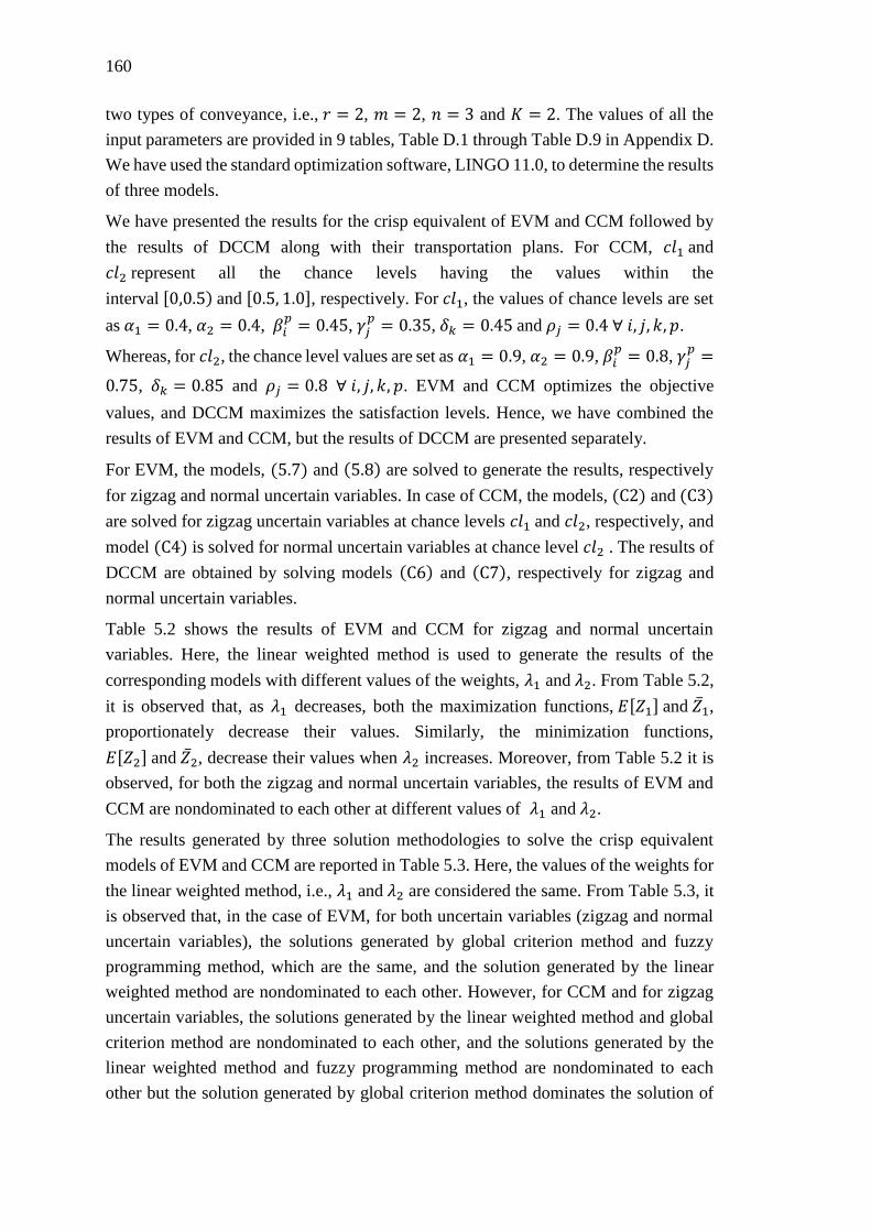
160

two types of conveyance, i.e., 𝑟 = 2, 𝑚 = 2, 𝑛 = 3 and 𝐾 = 2. The values of all the

input parameters are provided in 9 tables, Table D.1 through Table D.9 in Appendix D.

We have used the standard optimization software, LINGO 11.0, to determine the results

of three models.

We have presented the results for the crisp equivalent of EVM and CCM followed by

the results of DCCM along with their transportation plans. For CCM, 𝑐𝑙1 and

𝑐𝑙2 represent all the chance levels having the values within the

interval [0,0.5) and [0.5, 1.0], respectively. For 𝑐𝑙1, the values of chance levels are set

as 𝛼1 = 0.4, 𝛼2 = 0.4, 𝛽𝑖𝑝 = 0.45, 𝛾𝑗

𝑝 = 0.35, 𝛿𝑘 = 0.45 and 𝜌𝑗 = 0.4 ∀ 𝑖, 𝑗, 𝑘, 𝑝.

Whereas, for 𝑐𝑙2, the chance level values are set as 𝛼1 = 0.9, 𝛼2 = 0.9, 𝛽𝑖𝑝 = 0.8, 𝛾𝑗

𝑝 =

0.75, 𝛿𝑘 = 0.85 and 𝜌𝑗 = 0.8 ∀ 𝑖, 𝑗, 𝑘, 𝑝. EVM and CCM optimizes the objective

values, and DCCM maximizes the satisfaction levels. Hence, we have combined the

results of EVM and CCM, but the results of DCCM are presented separately.

For EVM, the models, (5.7) and (5.8) are solved to generate the results, respectively

for zigzag and normal uncertain variables. In case of CCM, the models, (C2) and (C3)

are solved for zigzag uncertain variables at chance levels 𝑐𝑙1 and 𝑐𝑙2, respectively, and

model (C4) is solved for normal uncertain variables at chance level 𝑐𝑙2 . The results of

DCCM are obtained by solving models (C6) and (C7), respectively for zigzag and

normal uncertain variables.

Table 5.2 shows the results of EVM and CCM for zigzag and normal uncertain

variables. Here, the linear weighted method is used to generate the results of the

corresponding models with different values of the weights, 𝜆1 and 𝜆2. From Table 5.2,

it is observed that, as 𝜆1 decreases, both the maximization functions, 𝐸[𝑍1] and ��1,

proportionately decrease their values. Similarly, the minimization functions,

𝐸[𝑍2] and ��2, decrease their values when 𝜆2 increases. Moreover, from Table 5.2 it is

observed, for both the zigzag and normal uncertain variables, the results of EVM and

CCM are nondominated to each other at different values of 𝜆1 and 𝜆2.

The results generated by three solution methodologies to solve the crisp equivalent

models of EVM and CCM are reported in Table 5.3. Here, the values of the weights for

the linear weighted method, i.e., 𝜆1 and 𝜆2 are considered the same. From Table 5.3, it

is observed that, in the case of EVM, for both uncertain variables (zigzag and normal

uncertain variables), the solutions generated by global criterion method and fuzzy

programming method, which are the same, and the solution generated by the linear

weighted method are nondominated to each other. However, for CCM and for zigzag

uncertain variables, the solutions generated by the linear weighted method and global

criterion method are nondominated to each other, and the solutions generated by the

linear weighted method and fuzzy programming method are nondominated to each

other but the solution generated by global criterion method dominates the solution of

161

fuzzy programming method. While, for CCM with normal uncertain variables, the

solutions generated by the linear weighted method, global criterion method and fuzzy

programming method are nondominated to each other. Here, Table 5.4 shows the

transportation plans corresponding to the results provided in Table 5.3, for EVM and

CCM.

Table 5.2 Optimum results of EVM and CCM for zigzag and normal uncertain

variables using linear weighted method

Weights

EVM CCM

𝑐𝑙1 𝑐𝑙2

𝜆1 𝜆2 E[𝑍1] E[𝑍2] ��1 ��2 ��1 ��2

Zigzag

uncertain

variables

1.0 0.0 526.125 87.500 572.327 86.719 346.414 102.481

0.7 0.3 526.125 87.500 570.600 85.120 346.414 102.481

0.5 0.5 513.250 75.250 570.600 85.120 344.440 100.800

0.3 0.7 509.419 73.742 554.440 72.940 326.175 93.154

0.0 1.0 334.375 69.700 315.980 62.420 268.580 90.740

Normal

uncertain

variables

𝑐𝑙2

��1 ��2

1.0 0.0 576.185 89.290 467.172 98.741

0.7 0.3 573.769 87.912 456.383 97.279

0.5 0.5 572.848 87.800 456.147 95.584

0.3 0.7 535.400 65.114 404.117 84.650

0.0 1.0 427.529 59.600 347.127 81.525

Table 5.3 Comparative results of three different solution methodologies

Solution method Model

EVM CCM

𝑐𝑙1 𝑐𝑙2

E[𝑍1] E[𝑍2] ��1 ��2 ��1 ��2

Zigzag

uncertain

variables

Linear weighted method

(with equal weights) 513.250 75.250 570.600 85.120 344.440 100.800

Global criterion method 495.750 72.425 542.220 70.180 315.500 94.860 Fuzzy programming

method 495.750 72.425 483.558 70.180 313.372 94.860

Normal

uncertain

variables

𝑐𝑙2

��1 ��2


(with equal weights) 572.848 87.800 456.147 95.584

Global criterion method 516.736 69.200 404.117 84.652 Fuzzy programming

method 516.736 69.200 409.800 87.736

For DCCM, the results for three solution methodologies are shown in Table 5.5. Similar

to Table 5.3, the associated weights of the linear weighted method in Table 5.5 are

considered equal. Moreover, to solve the crisp equivalents of DCCM, the

predetermined limits of 𝑍1′ and 𝑍2

′ , are set to, 325 and 94, respectively, for the

model (C6), and 419 and 83, respectively, for the model (C7). It is observed from

Table 5.5 that, for zigzag uncertain variables, the solution generated by the global

criterion method dominates each of the solutions generated by the linear weighted

method and fuzzy programming method. Moreover, the solution generated by the fuzzy

162

programming method dominates the solution generated by the linear weighted method.

However, for normal uncertain variables, the solutions generated by the linear weighted

method and global criterion method, which are the same, and the solution generated by

the fuzzy programming method are nondominated to each other. Here, Table 5.6 shows

the transportation plans corresponding to the results presented in Table 5.5, of DCCM,

for zigzag and normal uncertain variables.

Table 5.4 Optimal transportation plan of the EVM and CCM for normal uncertain

variables using three different solution methodologies

Model Solution method


(with equal weights)

Global criterion method Fuzzy programming

method

Zigzag

uncertain

variables

EVM 𝑥1211 =19.00, 𝑥132

1 =13.50,

𝑥2121 =31.50, 𝑥232

1 =5.75, 𝑥1212

=8.60,𝑥1312 =17.50, 𝑥212

2 =

13.73, 𝑥2222 =15.00

𝑥1121 =13.50, 𝑥121

1 =19.00,

𝑥2121 =18.00, 𝑥232

1 =19.25,

𝑥1312 =26.00,𝑥212

2 =13.75,

𝑥2222 =15.00

𝑥1121 =13.50, 𝑥121

1 =19.00,

𝑥2121 =18.00, 𝑥232

1 =19.25,

𝑥1312 =26.00,𝑥212

2 =13.75,

𝑥2222 =15.00

CCM

𝑐𝑙1

𝑥1211 =18.60, 𝑥132

1 =

13.70,𝑥2121 =32.70,

𝑥2321 =4.70, 𝑥121

2 =8.60,

𝑥1312 =17.50, 𝑥212

2 =

23.70, 𝑥2222 =5.50

𝑥1121 =13.70, 𝑥121

1 =18.60,

𝑥2121 =19.00, 𝑥232

1 =18.40,

𝑥1312 =26.10,𝑥212

2 =15.10,

𝑥2222 =14.10

𝑥1121 =16.20, 𝑥121

1 =16.10,

𝑥2121 =11.428, 𝑥232

1 =

18.40, 𝑥1312 =26.10,𝑥212

2 =

15.10, 𝑥2222 =14.10

𝑐𝑙2

𝑥1211 =19.00, 𝑥132

1 =

12.40,𝑥2121 =72.10,

𝑥2321 =8.10, 𝑥121

2 =5.40,

𝑥1312 =20. 00, 𝑥212

2 =

16.10, 𝑥2222 =11.10

𝑥1211 =20.60, 𝑥132

1 =10.80,

𝑥2121 =25.50, 𝑥232

1 =9.70, 𝑥1222

=3.30,𝑥1312 =22.10, 𝑥212

2 =

14.00, 𝑥2222 =13.20

𝑥1211 =20.60, 𝑥132

1 =10.80,

𝑥2121 =25.50, 𝑥232

1 =9.70,

𝑥1222 =3.30,𝑥131

2 =21.43,

𝑥2122 =14.00, 𝑥222

2 =13.20

Normal

uncertain

variables

EVM 𝑥1211 =17.84, 𝑥132

1 =14.15,

𝑥2121 =25.12, 𝑥232

1 =9.87, 𝑥1122

=11.00,𝑥1212 =14.00, 𝑥211

2 =

8.15, 𝑥2322 =19.84

𝑥1121 =16.00, 𝑥121

1 =16.00,

𝑥2121 =12.15, 𝑥232

1 =22.84,

𝑥1212 =21.21,𝑥212

2 =12.00,

𝑥2322 =16.00

𝑥1121 =16.00, 𝑥121

1 =16.00,

𝑥2121 =12.15, 𝑥232

1 =22.84,

𝑥1212 =21.21,𝑥212

2 =12.00,

𝑥2322 =16.00

CCM

𝑐𝑙2

𝑥1211 =16.46, 𝑥132

1 =7.15,

𝑥2121 =22.92, 𝑥232

1 =

11.41, 𝑥1122 =9. 17,𝑥121

2 =

14.50, 𝑥2122 =11. 07,

𝑥2322 =16.56

𝑥1121 =10.89, 𝑥121

1 =16. 46,

𝑥2121 =15.61, 𝑥232

1 =18.72,

𝑥1312 =23. 67,𝑥212

2 =13.14,

𝑥2222 =14.50

𝑥1211 =16.46, 𝑥132

1 =14. 34,𝑥2121 =30. 10, 𝑥232

1 =4.22,

𝑥1312 =19.53,𝑥212

2 =13.14,

𝑥2222 =14.50

We have analyzed the sensitivity of CCM with input parameters of UMMFSTPwB,

consider as zigzag and normal uncertain variables. The corresponding results of the

CCM are reported in Table 5.7. Here, the models for both the uncertain variables

(zigzag and normal uncertain variables) are solved, using the global criterion method,

by changing the values of the chance levels, 𝛼1 and 𝛼2. For zigzag uncertain variables,

model (𝐶2) is solved when the values of 𝛼1 and 𝛼2 change their respective values

between 0.1 to 0.4. In this case, all other chance levels except 𝛼1 and 𝛼2, are set

to, 𝛽𝑖𝑝 = 0.45, 𝛾𝑗

𝑝 = 0.35, 𝛿𝑘 = 0.45 and 𝜌𝑗 = 0.4. When the values of 𝛼1 and 𝛼2 are

changed within the range from 0.5 to 1.0, model (𝐶3) is solved with the remaining

chance levels set to, 𝛽𝑖𝑝 = 0.8, 𝛾𝑗

𝑝 = 0.75, 𝛿𝑘 = 0.85 and 𝜌𝑗 = 0.8. However, for

normal uncertain variables, model (𝐶4) is solved at different values of 𝛼1 and 𝛼2 by

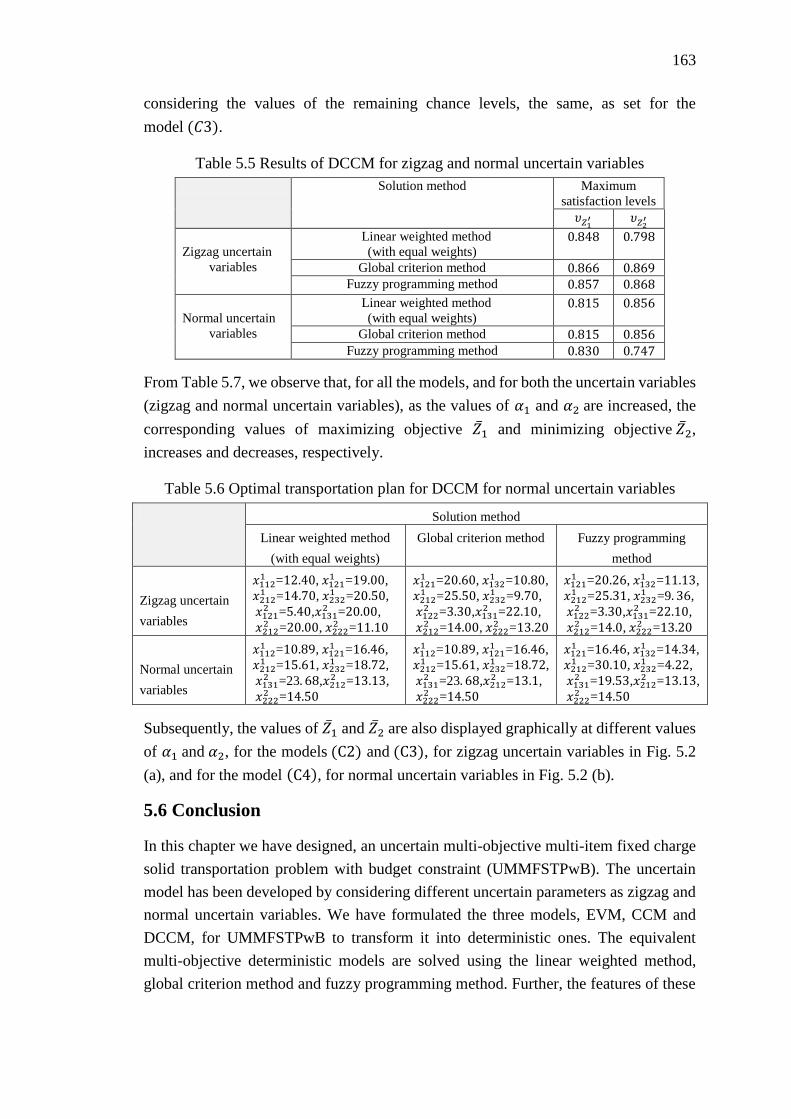
163

considering the values of the remaining chance levels, the same, as set for the

model (𝐶3).

Table 5.5 Results of DCCM for zigzag and normal uncertain variables

Solution method Maximum

satisfaction levels

𝜐𝑍1′ 𝜐𝑍2′

Zigzag uncertain

variables


(with equal weights) 0.848 0.798

Global criterion method 0.866 0.869 Fuzzy programming method 0.857 0.868

Normal uncertain

variables


(with equal weights) 0.815 0.856

Global criterion method 0.815 0.856 Fuzzy programming method 0.830 0.747

From Table 5.7, we observe that, for all the models, and for both the uncertain variables

(zigzag and normal uncertain variables), as the values of 𝛼1 and 𝛼2 are increased, the

corresponding values of maximizing objective ��1 and minimizing objective ��2,

increases and decreases, respectively.

Table 5.6 Optimal transportation plan for DCCM for normal uncertain variables

Solution method


(with equal weights)

Global criterion method Fuzzy programming

method

Zigzag uncertain

variables

𝑥1121 =12.40, 𝑥121

1 =19.00,

𝑥2121 =14.70, 𝑥232

1 =20.50,

𝑥1212 =5.40,𝑥131

2 =20.00,

𝑥2122 =20.00, 𝑥222

2 =11.10

𝑥1211 =20.60, 𝑥132

1 =10.80,

𝑥2121 =25.50, 𝑥232

1 =9.70,

𝑥1222 =3.30,𝑥131

2 =22.10,

𝑥2122 =14.00, 𝑥222

2 =13.20

𝑥1211 =20.26, 𝑥132

1 =11.13,

𝑥2121 =25.31, 𝑥232

1 =9. 36,

𝑥1222 =3.30,𝑥131

2 =22.10,

𝑥2122 =14.0, 𝑥222

2 =13.20

Normal uncertain

variables

𝑥1121 =10.89, 𝑥121

1 =16.46,

𝑥2121 =15.61, 𝑥232

1 =18.72,

𝑥1312 =23. 68,𝑥212

2 =13.13,

𝑥2222 =14.50

𝑥1121 =10.89, 𝑥121

1 =16.46,

𝑥2121 =15.61, 𝑥232

1 =18.72,

𝑥1312 =23. 68,𝑥212

2 =13.1,

𝑥2222 =14.50

𝑥1211 =16.46, 𝑥132

1 =14.34,

𝑥2121 =30.10, 𝑥232

1 =4.22,

𝑥1312 =19.53,𝑥212

2 =13.13,

𝑥2222 =14.50

Subsequently, the values of ��1 and ��2 are also displayed graphically at different values

of 𝛼1 and 𝛼2, for the models (C2) and (C3), for zigzag uncertain variables in Fig. 5.2

(a), and for the model (C4), for normal uncertain variables in Fig. 5.2 (b).

5.6 Conclusion

In this chapter we have designed, an uncertain multi-objective multi-item fixed charge

solid transportation problem with budget constraint (UMMFSTPwB). The uncertain

model has been developed by considering different uncertain parameters as zigzag and

normal uncertain variables. We have formulated the three models, EVM, CCM and

DCCM, for UMMFSTPwB to transform it into deterministic ones. The equivalent

multi-objective deterministic models are solved using the linear weighted method,

global criterion method and fuzzy programming method. Further, the features of these

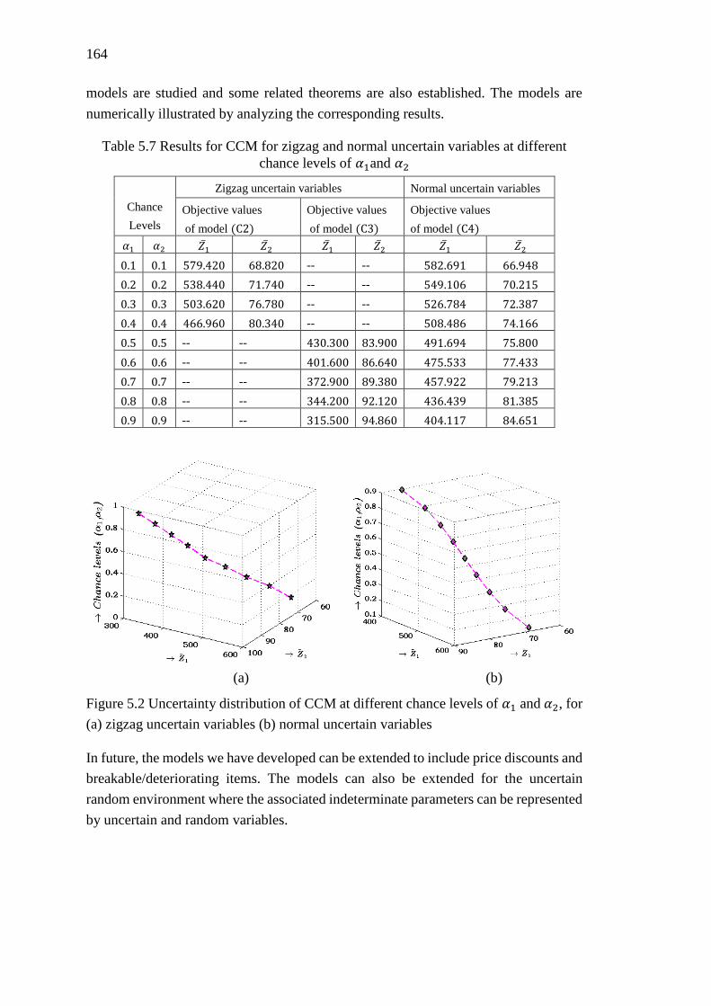
164

models are studied and some related theorems are also established. The models are

numerically illustrated by analyzing the corresponding results.

Table 5.7 Results for CCM for zigzag and normal uncertain variables at different

chance levels of 𝛼1and 𝛼2

(a) (b)

Figure 5.2 Uncertainty distribution of CCM at different chance levels of 𝛼1 and 𝛼2, for

(a) zigzag uncertain variables (b) normal uncertain variables

In future, the models we have developed can be extended to include price discounts and

breakable/deteriorating items. The models can also be extended for the uncertain

random environment where the associated indeterminate parameters can be represented

by uncertain and random variables.

Chance

Levels

Zigzag uncertain variables Normal uncertain variables

Objective values

of model (C2)

Objective values

of model (C3)

Objective values

of model (C4)

𝛼1 𝛼2 ��1 ��2 ��1 ��2 ��1 ��2

0.1 0.1 579.420 68.820 -- -- 582.691 66.948

0.2 0.2 538.440 71.740 -- -- 549.106 70.215

0.3 0.3 503.620 76.780 -- -- 526.784 72.387

0.4 0.4 466.960 80.340 -- -- 508.486 74.166

0.5 0.5 -- -- 430.300 83.900 491.694 75.800

0.6 0.6 -- -- 401.600 86.640 475.533 77.433

0.7 0.7 -- -- 372.900 89.380 457.922 79.213

0.8 0.8 -- -- 344.200 92.120 436.439 81.385

0.9 0.9 -- -- 315.500 94.860 404.117 84.651

165

Chapter 6

Multi-objective Rough Fuzzy Quadratic

Minimum Spanning Tree Problem

User

Text Box

166

User

Text Box

167

Chapter 6

Multi-objective Rough Fuzzy Quadratic

Minimum Spanning Tree Problem

6.1 Introduction

Minimum spanning tree (MST) problem is one of the most fundamental and important

problems in network optimization which has diverse applications in different

engineering and scientific domains. The MST problem is to find a minimally connected

sub-graph which spans all the vertices of a connected finite network. The quadratic

minimum spanning tree (QMST) problem is a variant of MST introduced by Assad and

Xu (1992), which determines a minimum spanning tree of a weighted connected

network by considering two types of weights: linear and quadratic. The linear weights

are associated with each edge and the quadratic weights, generally arise due to the

interaction effect between any pair of edges. The QMST problem has different

applications (Cordone and Passeri 2012) in network design including

telecommunication networks, oil or water transmission networks, transportation

networks, etc. In telecommunication networks, the linear weights represent the costs to

establish radio or cable connections, while the quadratic weights represent the cost of a

conversion device between different types of connected cables. In a utility network (oil

or water transmission networks) or a transportation network, the linear weights

represent the cost of installing different pipes, and the quadratic weights represent the

interaction/interfacing costs for installing valves or bending losses in T-joints. In a

transportation network, the linear and quadratic weights, respectively represent the cost

of constructing roads and turn penalties. In QMST, the interfacing costs mostly exist

for adjacent edges. However, sometimes these interfacing costs may also exist for any

pair of edges, but such topological design has little resemblance with physical layout,

as in the case of fiber-optic networks (Assad and Xu 1992; Cordone and Passeri 2012).

During the last few decades, QMST has been investigated by many researchers. Assad

and Xu (1992) incorporated the branch-and-bound method to determine the solutions

of the problem. Zhou and Gen (1998) proposed a genetic algorithm for QMST.

Palubeckis et al. (2010) presented the multi-start simulated annealing, hybrid genetic

algorithm and iterative tabu search algorithm to solve QMST problem. Sundar and

Singh (2010) solved it by an artificial bee colony algorithm. To solve the QMST

problem, Öncan and Punnen (2010) developed an efficient local search algorithm.

User

Text Box

168

Cordone and Passeri (2012) presented a tabu search and variable neighbourhood search

algorithms to solve the problem. A reformulation for QMST was introduced by Pereira

et al. (2013), which can compute stronger linear programming bounds. Lozano et al.

(2013) proposed the solution methodology for the QMST by incorporating the strategic

oscillation algorithm with tabu search. The authors presented an algorithm based on

dynamic column and row generation to evaluate the bounds. To solve the problem,

Rostami and Malucelli (2015) modelled some new mixed 0-1 linear formulations using

a reformulation-linearization technique. Later, Pereira et al. (2015) provided a new

formulation of the QMST and solved the problem using two parallel branch-and-bound

algorithms. Recently, Ćustić et al. (2018) investigated the polynomially and NP-hard

solvable instances of a connected network to determine QMST and its three variants:

(i) quadratic bottleneck spanning tree problem, (ii) minimum spanning tree problem

with conflict pair constraints and (iii) bottleneck spanning tree problem with conflict

pair constraints.

All the above mentioned studies on QMST are considered as a single objective

optimization problem, where the linear weights are added with the quadratic weights.

The conflicting nature of the linear and the quadratic weights have been studied by

Maia et al. (2013). Here, the authors have considered the linear and quadratic weights

as two separate objectives for the problem. In their study, a Pareto local search

algorithm has been proposed for a bi-objective QMST, where the quadratic weights are

considered for any pair of adjacent edges.

In many decision making problems, the associated parameters are not always exact but

are imprecise in nature due to inadequate information, lack of evidence, multiple input

sources, fluctuating nature of input parameters, measurement inaccuracy, etc.

Therefore, in order to process and represent the useful data hidden within the imprecise

or ill-defined information, many researchers have proposed several improved theories

like probability theory, fuzzy set (L.A. Zadeh 1965), rough set (Z. Pawlak 1982), and

uncertainty theory (B. Liu 2007). Some applications (Zhang et al. 2003; Feng et al.

2010; Sun et al. 2014a; Wang et al. 2016; Majumder et al. 2018; Zhou et al. 2018; Rani

and Garg 2018) of those theories are also observed in the literature.

Considering the uncertain MST problem, the stochastic MST has been studied by

various researchers (Swamy and Shmoys 2006; Torkestani and Meybodi 2012).

Similarly, some significant contributions on fuzzy MST (Janik and Kasperski 2008;

Zhou et al. 2016a; Gao et al. 2018) also exist in the literature. However, unlike uncertain

MST, not many investigations have been done for QMST with uncertain parameters.

At present, there are only two relevant studies on QMST problem under uncertain

environment. In the first study, Gao and Lu (2005) defined a QMST with linear and

quadratic fuzzy weights, and solved the problem using a genetic algorithm. Later, Zhou

169

et al. (2014b) defined a chance-constrained model for a QMST, where the linear and

quadratic weights are represented by uncertain variables (B. Liu 2007).

In some decision making process, a DM may need to take decisions under a two-fold

uncertain environment, where both roughness and fuzziness co-exist. In this context,

the concepts of rough fuzzy sets and fuzzy rough sets, introduced by Dubois and Prade

(1990), play an important role. In their study, the authors combined the fuzzy set and

rough set with an aim to fulfil two different objectives. The first one is to determine the

lower and upper approximations of the fuzzy set, and the second one is to replace the

equivalence relation of the rough set with the fuzzy similarity relation. Since then, some

important contributions on the hybridization of fuzzy and rough sets have been

observed both in theory (Li and Zhang 2008; Yang and Hinde 2010; Y. Cheng 2015;

M. Diker 2018; Qiao and Hu 2018) and in applications (Wu et al. 2003; Liu et al. 2014b;

Sun et al. 2014b; Lin et al. 2018; Zhang et al. 2018) domains. Motivated by the study

of Dubois and Prade (1990), B. Liu (2002) introduced the concept of rough fuzzy

variable and developed it further in B. Liu (2004). In reality, the parameters in some

decision making problems may be uncertain and can be represented by rough fuzzy

variable. For instance, the transportation cost (𝑐𝑡) depends upon fuel price, toll tax,

vehicle maintenance cost, etc., each of which fluctuates from time to time. In general,

the possible parameter values are provided by experts in terms of approximate intervals.

As an example, let the transportation cost while traversing a route, in a particular month,

as estimated by experts is “between $ 70- $ 80”, which can be represented by a rough

variable (B. Liu 2002). However, each point within the intervals of a rough variable

may not be equipossible and can be “around $ 74”. It may be because 𝑐𝑡 may differ

throughout the months in a year due to the fluctuation of fuel price, toll charges, etc.

Therefore, such type of linguistic information can be approximated by rough fuzzy

variables, and accordingly 𝑐𝑡 can be represented by a rough fuzzy transportation

cost 휁𝑐𝑡 , where 휁𝑐𝑡 = [𝜉, 𝜉 + 2][𝜉 − 2, 𝜉 + 4], 𝜉 = (72, 74, 76 ).

Considering the existing studies on QMST and some recent studies on rough fuzzy set,

we observe that there are some lacunas in the literature which are mentioned below.

(i) Any optimization problem with associated parameters as rough fuzzy variables

is yet to be studied in the literature.

(ii) A bi-objective QMST problem under rough fuzzy uncertain environments is not

yet considered in the literature.

In order to address the above mentioned lacunas, in the present study, we have

considered a bi-objective rough fuzzy quadratic minimum spanning tree problem (b-

RFQMSTP), by considering the linear and quadratic weights as rough fuzzy variables.

The bi-objective QMST problem is modelled using rough fuzzy chance-constrained

programming (RFCCP) technique. It is solved by epsilon-constraint method (Hames et

al. 1971), which is a classical multi-objective programming technique, and two multi-

170

objective genetic algorithms (MOGAs): (i) nondominated sorting algorithm II (NSGA-

II) (Deb et al. 2002) and (ii) multi-objective cross generational elitist selection,

heterogeneous recombination, and cataclysmic mutation (MOCHC) (Nebro et al.

2007).

The rest of the chapter is organized as follows. Some related theorems of a multi-

objective optimization problem with rough fuzzy parameters are presented in Section

6.2. The proposed chance-constrained model and its crisp equivalents are formulated in

Section 6.3. A numerical example is illustrated in Section 6.4. The discussions of the

results, of the proposed model, are provided in Section 6.5. In Section 6.6, we have

presented a case study to numerically illustrate the proposed b-RFQMSTP. Finally, we

conclude the study in Section 6.7.

6.2 Multi-objective Model with Rough Fuzzy Coefficients

A rough fuzzy multi-objective problem (RFMOP) deals with optimizing a vector of

conflicting objectives subject to a set of constraints, where the associated coefficients

of the objectives and constraints are rough fuzzy variables. An RFMOP model is

defined below in (6.1).

{

𝑀𝑖𝑛𝑖𝑚𝑖𝑧𝑒 (𝑓1(휁1𝑇 , 𝒳), 𝑓2(휁2

𝑇 , 𝒳), … , 𝑓𝑚(휁𝑚𝑇 , 𝒳))


𝑔𝑖(휁𝑖𝑇 , 𝒳) ≤ 0; 𝑖 = 1,2, … , 𝑝,

(6.1)

where, 𝑚 is the number of objective functions, 𝒳 = (𝑥1, 𝑥2, … , 𝑥𝑛)𝑇 is the decision

vector. 휁𝑙𝑇 = (휁𝑙1, 휁𝑙2, … , 휁𝑙𝑛)

𝑇𝑙 = 1,2, … ,𝑚 and 휁𝑖

𝑇 = (휁𝑖1, 휁𝑖2, … , 휁𝑖𝑛)𝑇; 𝑖 = 1,2, . . . , 𝑝

are the rough fuzzy vectors.

Following Definition 1.3.26 (cf. Section 1.3.10), from (6.1), the primitive chance of

𝑔𝑖(휁𝑖𝑇 , 𝒳) ≤ 0 can be stated as

𝐶ℎ{𝑔𝑖(휁𝑖𝑇 , 𝒳) ≤ 0}(𝛽𝑖) ≥ 𝛼𝑖 = 𝐶𝑟{휃 ∈ Θ|𝑇𝑟{𝑔𝑖(휁𝑖

𝑇 , 𝒳) ≤ 0} ≥ 𝛼𝑖} ≥ 𝛽𝑖, 𝑖 =

1,2, … , 𝑝, and 𝐶ℎ{𝑓𝑙(휁𝑙𝑇 , 𝒳) ≤ 𝑓��}(𝜏𝑙) ≥ 𝜌𝑙 = 𝐶𝑟{휃 ∈ Θ|𝑇𝑟{𝑓𝑙(휁𝑙

𝑇 , 𝒳) ≤ 𝑓��} ≥ 𝜌𝑙} ≥

𝜏𝑙, 𝑙 = 1,2, … ,𝑚.

Furthermore, a decision vector 𝒳 is said to be feasible to (6.1) if and only if the

credibility measures of the fuzzy events, {휃 ∈ Θ|𝑇𝑟{𝑓𝑙(휁𝑙𝑇 , 𝒳) ≤ 𝑓��} ≥ 𝜌𝑙} at

confidence levels of at least 𝜏𝑙, are satisfied by a set of fuzzy event,

{휃 ∈ Θ|𝑇𝑟{𝑔𝑖(휁𝑖𝑇 , 𝒳) ≤ 0} ≥ 𝛼𝑖} having at least credibility measures 𝛽𝑖.

Hence, the chance-constrained multi-objective programming model can be formulated

as presented in (6.2).

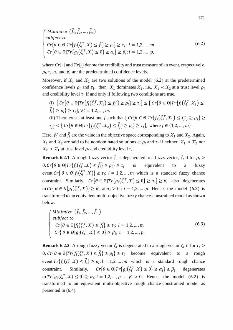
171

{

𝑀𝑖𝑛𝑖𝑚𝑖𝑧𝑒 (𝑓1, 𝑓2, … , 𝑓��)


𝐶𝑟{휃 ∈ Θ|𝑇𝑟{𝑓𝑙(휁𝑙 𝑇 , 𝒳) ≤ 𝑓��} ≥ 𝜌𝑙} ≥ 𝜏𝑙; 𝑙 = 1,2, … ,𝑚

𝐶𝑟{휃 ∈ Θ|𝑇𝑟{𝑔𝑖(휁𝑖 𝑇 , 𝒳) ≤ 0} ≥ 𝛼𝑖} ≥ 𝛽𝑖; 𝑖 = 1,2, … , 𝑝,

(6.2)

where 𝐶𝑟{·} and 𝑇𝑟{·} denote the credibility and trust measure of an event, respectively.

𝜌𝑙 , 𝜏𝑙, 𝛼𝑖 and 𝛽𝑖 are the predetermined confidence levels.

Moreover, if 𝒳1 and 𝒳2 are two solutions of the model (6.2) at the predetermined

confidence levels 𝜌𝑙 and 𝜏𝑙, then 𝒳1 dominates 𝒳2, i.e., 𝒳1 ≺ 𝒳2 at a trust level 𝜌𝑙

and credibility level 𝜏𝑙 if and only if following two conditions are true.

(i) { 𝐶𝑟{휃 ∈ Θ|𝑇𝑟{𝑓𝑙(휁𝑙 𝑇 , 𝒳1) ≤ 𝑓𝑙

∗} ≥ 𝜌𝑙} ≥ 𝜏𝑙} ≤ { 𝐶𝑟{휃 ∈ Θ|𝑇𝑟{𝑓𝑙(휁𝑙 𝑇 , 𝒳2) ≤

𝑓��} ≥ 𝜌𝑙} ≥ 𝜏𝑙}, ∀𝑙 = 1,2, … ,𝑚.

(ii) There exists at least one 𝑗 such that { 𝐶𝑟{휃 ∈ Θ|𝑇𝑟{𝑓𝑗(휁𝑗 𝑇 , 𝒳1) ≤ 𝑓𝑗

∗} ≥ 𝜌𝑗} ≥

𝜏𝑗} < { 𝐶𝑟{휃 ∈ Θ|𝑇𝑟{𝑓𝑗(휁𝑗 𝑇 , 𝒳2) ≤ 𝑓��} ≥ 𝜌𝑙} ≥ 𝜏𝑙}, where 𝑗 ∈ {1,2, … ,𝑚}

Here, 𝑓𝑙∗ and 𝑓�� are the value in the objective space corresponding to 𝒳1 and 𝒳2. Again,

𝒳1 and 𝒳2 are said to be nondominated solutions at 𝜌𝑙 and 𝜏𝑙 if neither 𝒳1 ≺ 𝒳2 nor

𝒳2 ≺ 𝒳1 at trust level 𝜌𝑙 and credibility level 𝜏𝑙 .

Remark 6.2.1: A rough fuzzy vector 휁𝑙 is degenerated to a fuzzy vector, 휁𝑙 if for 𝜌𝑙 >

0, 𝐶𝑟{휃 ∈ Θ|𝑇𝑟{𝑓𝑙(휁𝑙𝑇 , 𝒳) ≤ 𝑓��} ≥ 𝜌𝑙} ≥ 𝜏𝑙 is equivalent to a fuzzy

event 𝐶𝑟{ 휃 ∈ 𝛩|𝑓𝑙(휁𝑙 𝑇 , 𝒳)} ≥ 𝜏𝑙; 𝑙 = 1,2, … ,𝑚 which is a standard fuzzy chance

constraint. Similarly, 𝐶𝑟{휃 ∈ Θ|𝑇𝑟{𝑔𝑖(휁𝑖 𝑇 , 𝒳) ≤ 0} ≥ 𝛼𝑖} ≥ 𝛽𝑖 also degenerates

to 𝐶𝑟{ 휃 ∈ 𝛩|𝑔𝑖(휁𝑖 𝑇 , 𝒳)} ≥ 𝛽𝑖 at 𝛼𝑖 > 0 ; 𝑖 = 1,2, … , 𝑝. Hence, the model (6.2) is

transformed to an equivalent multi-objective fuzzy chance-constrained model as shown

below.

{



𝐶𝑟{휃 ∈ Θ|𝑓𝑙(휁𝑙 𝑇 , 𝒳) ≤ 𝑓��} ≥ 𝜏𝑙; 𝑙 = 1,2, … ,𝑚

𝐶𝑟{ 휃 ∈ 𝛩|𝑔𝑖(휁𝑙 𝑇 , 𝒳) ≤ 0} ≥ 𝛽𝑖; 𝑖 = 1,2, … , 𝑝.

(6.3)

Remark 6.2.2: A rough fuzzy vector 휁𝑙 is degenerated to a rough vector 휁𝑙 if for 𝜏𝑙 >

0, 𝐶𝑟{휃 ∈ Θ|𝑇𝑟{𝑓𝑙(휁𝑙𝑇 , 𝒳) ≤ 𝑓��} ≥ 𝜌𝑙} ≥ 𝜏𝑙 become equivalent to a rough

event 𝑇𝑟{𝑓𝑙(휁𝑙𝑇 , 𝒳) ≤ 𝑓��} ≥ 𝜌𝑙; 𝑙 = 1,2, … ,𝑚 which is a standard rough chance

constraint. Similarly, 𝐶𝑟{휃 ∈ Θ|𝑇𝑟{𝑔𝑖(휁𝑖 𝑇 , 𝒳) ≤ 0} ≥ 𝛼𝑖} ≥ 𝛽𝑖 degenerates

to 𝑇𝑟{𝑔𝑖(휁𝑖 𝑇 , 𝒳) ≤ 0} ≥ 𝛼𝑖; 𝑖 = 1,2, … , 𝑝 at 𝛽𝑖 > 0. Hence, the model (6.2) is

transformed to an equivalent multi-objective rough chance-constrained model as

presented in (6.4).

172

{



𝑇𝑟{𝑓𝑙(휁𝑙𝑇 , 𝒳) ≤ 𝑓��} ≥ 𝜌𝑙; 𝑙 = 1,2, … ,𝑚

𝑇𝑟{𝑔𝑖(휁𝑖 𝑇 , 𝒳) ≤ 0} ≥ 𝛼𝑖; 𝑖 = 1,2, … , 𝑝.

(6.4)

Lemma 6.2.1: For any 휃 ∈ Θ, a rough fuzzy vector 휁𝑖𝑗𝜒, degenerated to a fuzzy vector

휁𝑖(휃)𝑇𝜒 which takes the form of a fuzzy variable (𝑢, 𝑣, 𝑤), where 휁𝑖(휃) =

[휁𝑖1(휃), 휁𝑖2(휃),… , 휁𝑖𝑛(휃)]𝑇 and 𝜒 = [𝑥1, 𝑥2, … , 𝑥𝑛]

𝑇 are respectively a fuzzy vector and

decision vector.

Proof: Without loss of generality, for any 휃 ∈ Θ, we have assumed that a fuzzy variable

degenerated from a rough fuzzy variable becomes a triangular fuzzy variable. Let 휁𝑖𝑗

be a rough fuzzy variable, then for any 휃 ∈ Θ there exists a fuzzy variable 휁𝑖𝑗(휃) =

(𝑙𝑖𝑗, 𝑟𝑖𝑗 , 𝑠𝑖𝑗), 𝑙𝑖𝑗 < 𝑟𝑖𝑗 < 𝑠𝑖𝑗 with credibility measures defined as

𝐶𝑟(휁𝑖𝑗(휃) ≤ 𝑦) =

{

1 ; 𝑖𝑓 𝑠𝑖𝑗 < 𝑦 𝑦+𝑠𝑖𝑗−2𝑟𝑖𝑗

2(𝑠𝑖𝑗−𝑟𝑖𝑗) ; 𝑖𝑓 𝑟𝑖𝑗 < 𝑦 ≤ 𝑠𝑖𝑗

𝑦−𝑙𝑖𝑗

2(𝑟𝑖𝑗−𝑙𝑖𝑗) ; 𝑖𝑓 𝑙𝑖𝑗 ≤ 𝑦 ≤ 𝑟𝑖𝑗


and 𝐶𝑟(휁𝑖𝑗(휃) ≥ 𝑦) =

{

1 ; 𝑖𝑓 𝑦 < 𝑙𝑖𝑗2𝑟𝑖𝑗−𝑙𝑖𝑗−𝑦

2(𝑟𝑖𝑗−𝑙𝑖𝑗) ; 𝑖𝑓 𝑙𝑖𝑗 ≤ 𝑦 < 𝑟𝑖𝑗

𝑠𝑖𝑗−𝑦

2(𝑠𝑖𝑗−𝑟𝑖𝑗) ; 𝑖𝑓 𝑟𝑖𝑗 ≤ 𝑦 ≤ 𝑠𝑖𝑗


Subsequently, it follows

휁𝑖(휃)𝑇𝒳 =

∑ 휁𝑖𝑗(휃)𝒳𝑛𝑗=1 =(∑ (𝑙𝑖𝑗𝒳𝑗 , 𝑟𝑖𝑗𝒳𝑗 , 𝑠𝑖𝑗𝒳𝑗)

𝑛𝑗=1 )=(∑ 𝑙𝑖𝑗𝒳𝑗 , ∑ 𝑟𝑖𝑗𝒳𝑗

𝑛𝑗=1 , ∑ 𝑠𝑖𝑗𝒳𝑗

𝑛𝑗=1

𝑛𝑗=1 )

= (𝑢, 𝑣, 𝑤), where 𝑢 = ∑ 𝑙𝑖𝑗𝒳𝑗 ,𝑛𝑗=1 𝑣 = ∑ 𝑟𝑖𝑗𝒳𝑗

𝑛𝑗=1 and 𝑤 = ∑ 𝑠𝑖𝑗𝒳𝑗

𝑛𝑗=1 .

Lemma 6.2.2: For any 휃 ∈ Θ, a rough fuzzy vector 휁𝑖𝑗𝒳, degenerated to a rough vector

휁𝑖(휃)𝑇𝒳 which takes the form of a rough variable [𝑚, 𝑛], [𝑝, 𝑞], where 휁𝑖(휃)

𝑇 =

[휁𝑖1(휃), 휁𝑖2(휃),… , 휁𝑖𝑛(휃)]𝑇 and 𝒳 = [𝑥1, 𝑥2, … , 𝑥𝑛]

𝑇 are respectively, a rough vector

and a decision vector.

Proof: For a given 휃 ∈ Θ, a rough fuzzy variable 휁𝑖𝑗 when degenerated to a rough

variable 휁𝑖𝑗(휃) = [𝑢𝑖𝑗 , 𝑣𝑖𝑗][𝑠𝑖𝑗, 𝑡𝑖𝑗] , 𝑠𝑖𝑗 ≤ 𝑢𝑖𝑗 ≤ 𝑣𝑖𝑗 ≤ 𝑡𝑖𝑗 with trust distributions

173

𝑇𝑟{휁𝑖𝑗(휃) ≤ 𝑧} =

{

0 ; 𝑖𝑓 𝑧 ≤ 𝑠𝑖𝑗𝑧−𝑠𝑖𝑗

2(𝑡𝑖𝑗−𝑠𝑖𝑗) ; 𝑖𝑓 𝑠𝑖𝑗 ≤ 𝑧 ≤ 𝑢𝑖𝑗

1

2(𝑧−𝑢𝑖𝑗

𝑣𝑖𝑗−𝑢𝑖𝑗+

𝑧−𝑠𝑖𝑗

𝑡𝑖𝑗−𝑠𝑖𝑗) ; 𝑖𝑓 𝑢𝑖𝑗 ≤ 𝑧 ≤ 𝑣𝑖𝑗

1

2(𝑧−𝑠𝑖𝑗

𝑡𝑖𝑗−𝑠𝑖𝑗+ 1) ; 𝑖𝑓 𝑣𝑖𝑗 ≤ 𝑧 ≤ 𝑡𝑖𝑗

1 ; 𝑖𝑓 𝑧 ≥ 𝑡𝑖𝑗

and 𝑇𝑟{휁𝑖𝑗(휃) ≥ 𝑧} =

{

0 ; 𝑖𝑓 𝑧 ≥ 𝑞𝑡𝑖𝑗−𝑧

2(𝑡𝑖𝑗−𝑠𝑖𝑗) ; 𝑖𝑓 𝑣𝑖𝑗 ≤ 𝑧 ≤ 𝑡𝑖𝑗

1

2(𝑡𝑖𝑗−𝑧

𝑡𝑖𝑗−𝑠𝑖𝑗+

𝑣𝑖𝑗−𝑧

𝑣𝑖𝑗−𝑢𝑖𝑗) ; 𝑖𝑓 𝑢𝑖𝑗 ≤ 𝑧 ≤ 𝑣𝑖𝑗

1

2(𝑡𝑖𝑗−𝑧

𝑡𝑖𝑗−𝑠𝑖𝑗+ 1) ; 𝑖𝑓 𝑠𝑖𝑗 ≤ 𝑧 ≤ 𝑢𝑖𝑗

1 ; 𝑖𝑓 𝑧 ≤ 𝑠𝑖𝑗

Then, 휁𝑖(휃)𝑇𝒳 = ∑ 휁𝑖𝑗(휃)𝒳

𝑛𝑗=1 = ∑ ([𝑢𝑖𝑗𝒳𝑗 , 𝑣𝑖𝑗𝒳𝑗], [𝑠𝑖𝑗𝒳𝑗 , 𝑡𝑖𝑗𝒳𝑗])

𝑛𝑗=1

= ([∑ 𝑢𝑖𝑗𝒳𝑗𝑛𝑗=1 , ∑ 𝑣𝑖𝑗𝒳𝑗

𝑛𝑗=1 ], [∑ 𝑠𝑖𝑗𝒳𝑗

𝑛𝑗=1 , ∑ 𝑡𝑖𝑗𝒳𝑗

𝑛𝑗=1 ]) = [𝑚, 𝑛], [𝑝, 𝑞], where 𝑝 ≤

𝑚 ≤ 𝑛 ≤ 𝑞 such that 𝑚 = ∑ 𝑢𝑖𝑗𝒳𝑗𝑛𝑗=1 , 𝑛 = ∑ 𝑣𝑖𝑗𝒳𝑗

𝑛𝑗=1 , 𝑝 = ∑ 𝑠𝑖𝑗𝒳𝑗

𝑛𝑗=1 and 𝑞 =

∑ 𝑡𝑖𝑗𝒳𝑗𝑛𝑗=1 .

Theorem 6.2.1: For given confidence levels 𝛼𝑖, 𝛽𝑖 ∈ [0,1], when 𝑝 ≤ 𝑓�� ≤ 𝑚,

𝐶𝑟{휃 ∈ Θ|𝑇𝑟{휁𝑖(휃)𝑇𝒳 ≤ 𝑓��} ≥ 𝛼𝑖} ≥ 𝛽𝑖 implies 𝐶𝑟{휃 ∈ Θ|𝑝 + 2𝛼𝑖𝑄1 ≤ 𝑓��} ≥

𝛽𝑖, where 𝑄1 = (𝑞 − 𝑝).

Proof: From the result of Lemma 6.2.2, 휁𝑖(휃)𝑇𝒳 is known to be a rough variable.

Therefore, when 𝑝 ≤ 𝑓�� ≤ 𝑚, the trust distribution of 휁𝑖(휃)𝑇𝒳 is given below.

𝑇𝑟{휁𝑖(휃)𝑇𝒳 ≤ 𝑓��} =

{

0 ; 𝑓�� ≤ 𝑝

0.5��𝑖−𝑝

(𝑞−𝑝) ; 𝑝 ≤ 𝑓�� ≤ 𝑚

0.5 (��𝑖−𝑚

𝑛−𝑚+��𝑖−𝑝

𝑞−𝑝) ;𝑚 ≤ 𝑓�� ≤ 𝑛

0.5 (��𝑖−𝑝

𝑞−𝑝+ 1) ; 𝑛 ≤ 𝑓�� ≤ 𝑞

1 ; 𝑓�� ≥ 𝑞

⇒ 𝛼𝑖 ≤

{

0 ; 𝑓�� ≤ 𝑝

0.5��𝑖−𝑝

(𝑞−𝑝) ; 𝑝 ≤ 𝑓�� ≤ 𝑚

0.5 (��𝑖−𝑚

𝑛−𝑚+��𝑖−𝑝

𝑞−𝑝) ;𝑚 ≤ 𝑓�� ≤ 𝑛

0.5 (��𝑖−𝑝

𝑞−𝑝+ 1) ; 𝑛 ≤ 𝑓�� ≤ 𝑞

1 ; 𝑓�� ≥ 𝑞,

174

where 𝛼𝑖 is the predetermined confidence level of the trust distribution for the rough

variable 휁𝑖(휃)𝑇𝒳. It immediately follows that

𝑓�� ≥ 𝑝 + 2𝛼𝑖(𝑞 − 𝑝) if 𝑝 ≤ 𝑓�� ≤ 𝑚

𝑓�� ≥𝑚𝑞+𝑝𝑛+2𝛼𝑖(𝑛−𝑚)(𝑞−𝑝)−2𝑝𝑚

𝑛+𝑞−(𝑝+𝑚) if 𝑚 ≤ 𝑓�� ≤ 𝑛

and

𝑓�� ≥ 2𝑝 − 𝑞 + 2𝛼𝑖(𝑞 − 𝑝),if 𝑛 ≤ 𝑓�� ≤ 𝑞.

Therefore, we get

𝐶𝑟{휃 ∈ Θ|𝑇𝑟{휁𝑖(휃)𝑇𝒳 ≤ 𝑓��} ≥ 𝛼𝑖} ≥ 𝛽𝑖

⇒ 𝐶𝑟

{

휃 ∈ Θ|𝑓�� ≥

{

𝑝 + 2𝛼𝑖

(𝑞 − 𝑝) ; 𝑝 ≤ 𝑓�� ≤ 𝑚𝑚𝑞+𝑝𝑛+2𝛼𝑖(𝑛−𝑚)(𝑞−𝑝)−2𝑝𝑚

𝑛+𝑞−(𝑝+𝑚) ; 𝑚 ≤ 𝑓�� ≤ 𝑛

2𝑝 − 𝑞 + 2𝛼𝑖(𝑞 − 𝑝) ; 𝑛 ≤ 𝑓�� ≤ 𝑞

𝑞 ; 𝑞 ≤ 𝑓�� }

≥ 𝛽𝑖

⇒ 𝐶𝑟

{

휃 ∈ Θ|𝑓�� ≥

{

𝑝 + 2𝛼𝑖𝑄1 ; 𝑝 ≤ 𝑓�� ≤ 𝑚𝑚𝑞+𝑝𝑛+2𝛼𝑖𝑄2−2𝑝𝑚

𝑛+𝑞−(𝑝+𝑚) ; 𝑚 ≤ 𝑓�� ≤ 𝑛

2𝑝 − 𝑞 + 2𝛼𝑖𝑄1 ; 𝑛 ≤ 𝑓�� ≤ 𝑞

𝑞 ; 𝑞 ≤ 𝑓�� , }

≥ 𝛽𝑖

where 𝑄1 = (𝑞 − 𝑝) and 𝑄2 = (𝑛 −𝑚)(𝑞 − 𝑝).

Hence, when 𝑝 ≤ 𝑓�� ≤ 𝑚, it follows from the above result that 𝐶𝑟{휃 ∈

Θ|𝑇𝑟{휁𝑖(휃)𝑇𝒳 ≤ 𝑓��} ≥ 𝛼𝑖} ≥ 𝛽𝑖 ⇒ 𝐶𝑟{휃 ∈ Θ|𝑝 + 2𝛼𝑖𝑄1 ≤ 𝑓��} ≥ 𝛽𝑖, where 𝑄1 =

(𝑞 − 𝑝).

Theorem 6.2.2: For given confidence levels 𝛼𝑖 , 𝛽𝑖 ∈ [0,1], when 𝑝 ≤ 𝑓�� ≤ 𝑚,

𝐶𝑟{휃 ∈ Θ|𝑇𝑟{휁𝑖(휃)𝑇𝒳 ≤ 𝑓��} ≥ 𝛼𝑖} ≥ 𝛽𝑖 implies

𝑓��≥

{

𝑤 + 2𝛼𝑖𝑤𝑄1 ; 𝑖𝑓 𝑤 ≤ 𝑓�� − 2𝛼𝑖𝑄1

2(𝑣 + 𝛼𝑖𝑣𝑄1) − (𝑤 + 2𝛼𝑖𝑤𝑄1) + 2𝛽𝑖 ((𝑤 + 2𝛼𝑖𝑤𝑄1) − (𝑣 + 2𝛼𝑖𝑣𝑄1)) ; 𝑖𝑓 𝑣 ≤ 𝑓�� − 2𝛼𝑖𝑄1 ≤ 𝑤

𝑢 + 2𝛼𝑖𝑢𝑄1 + 2𝛽𝑖 ((𝑣 + 2𝛼𝑖𝑣𝑄1) − (𝑢 + 2𝛼𝑖𝑢𝑄1))) ; 𝑖𝑓 𝑢 ≤ 𝑓�� − 2𝛼𝑖𝑄1 ≤ 𝑣,

such that 𝑄1 = (𝑞 − 𝑝) is a triangular fuzzy variable of the form (𝑢𝑄1 , 𝑣𝑄1 , 𝑤𝑄1).

Proof: From the result of Theorem 6.2.1, 𝐶𝑟{휃 ∈ Θ|𝑇𝑟{휁𝑖(휃)𝑇𝒳 ≤ 𝑓��} ≥ 𝛼𝑖} ≥ 𝛽𝑖 ⇒

𝐶𝑟{휃 ∈ Θ|𝑝 + 2𝛼𝑖𝑄1 ≤ 𝑓��} ≥ 𝛽𝑖 when 𝑝 ≤ 𝑓�� ≤ 𝑚 and 𝑄1 = (𝑞 − 𝑝). Now 𝑝 and 𝑄1

are assumed to be triangular fuzzy variables of the form (𝑢, 𝑣, 𝑤) (cf. Lemma 6.2.1).

Thus

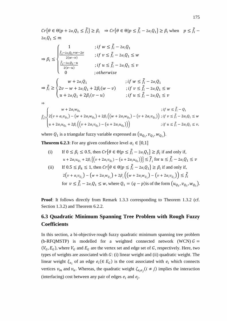
175

𝐶𝑟{휃 ∈ Θ|𝑝 + 2𝛼𝑖𝑄1 ≤ 𝑓��} ≥ 𝛽𝑖 ⇒ 𝐶𝑟{휃 ∈ Θ|𝑝 ≤ 𝑓�� − 2𝛼𝑖𝑄1} ≥ 𝛽𝑖 when 𝑝 ≤ 𝑓�� −

2𝛼𝑖𝑄1 ≤ 𝑚

⇒ 𝛽𝑖 ≤

{

1 ; 𝑖𝑓 𝑤 ≤ 𝑓�� − 2𝛼𝑖𝑄1��𝑖−2𝛼𝑖𝑄1+𝑤−2𝑣

2(𝑤−𝑣) ; 𝑖𝑓 𝑣 ≤ 𝑓�� − 2𝛼𝑖𝑄1 ≤ 𝑤

��𝑖−2𝛼𝑖𝑄1−𝑢

2(𝑣−𝑢) ; 𝑖𝑓 𝑢 ≤ 𝑓�� − 2𝛼𝑖𝑄1 ≤ 𝑣


⇒ 𝑓�� ≥ {

𝑤 + 2𝛼𝑖𝑄1 ; 𝑖𝑓 𝑤 ≤ 𝑓�� − 2𝛼𝑖𝑄1

2𝑣 − 𝑤 + 2𝛼𝑖𝑄1 + 2𝛽𝑖(𝑤 − 𝑣) ; 𝑖𝑓 𝑣 ≤ 𝑓�� − 2𝛼𝑖𝑄1 ≤ 𝑤

𝑢 + 2𝛼𝑖𝑄1 + 2𝛽𝑖(𝑣 − 𝑢) ; 𝑖𝑓 𝑢 ≤ 𝑓�� − 2𝛼𝑖𝑄1 ≤ 𝑣

⇒

𝑓��≥

{

𝑤 + 2𝛼𝑖𝑤𝑄1 ; 𝑖𝑓 𝑤 ≤ 𝑓�� − 𝑄1

2(𝑣 + 𝛼𝑖𝑣𝑄1) − (𝑤 + 2𝛼𝑖𝑤𝑄1) + 2𝛽𝑖 ((𝑤 + 2𝛼𝑖𝑤𝑄1) − (𝑣 + 2𝛼𝑖𝑣𝑄1)) ; 𝑖𝑓 𝑣 ≤ 𝑓�� − 2𝛼𝑖𝑄1 ≤ 𝑤

𝑢 + 2𝛼𝑖𝑢𝑄1 + 2𝛽𝑖 ((𝑣 + 2𝛼𝑖𝑣𝑄1) − (𝑢 + 2𝛼𝑖𝑢𝑄1))) ; 𝑖𝑓 𝑢 ≤ 𝑓�� − 2𝛼𝑖𝑄1 ≤ 𝑣,

where 𝑄1 is a triangular fuzzy variable expressed as (𝑢𝑄1 , 𝑣𝑄1 , 𝑤𝑄1).

Theorem 6.2.3: For any given confidence level 𝛼𝑖 ∈ [0,1]

(i) If 0 ≤ 𝛽𝑖 ≤ 0.5, then 𝐶𝑟{휃 ∈ Θ|𝑝 ≤ 𝑓�� − 2𝛼𝑖𝑄1} ≥ 𝛽𝑖 if and only if,

𝑢 + 2𝛼𝑖𝑢𝑄1 + 2𝛽𝑖 {(𝑣 + 2𝛼𝑖𝑣𝑄1) − (𝑢 + 2𝛼𝑖𝑢𝑄1))} ≤ ��𝑖 for 𝑢 ≤ 𝑓�� − 2𝛼𝑖𝑄1 ≤ 𝑣

(ii) If 0.5 ≤ 𝛽𝑘 ≤ 1, then 𝐶𝑟{휃 ∈ Θ|𝑝 ≤ 𝑓�� − 2𝛼𝑖𝑄1} ≥ 𝛽𝑖 if and only if,

2(𝑣 + 𝛼𝑖𝑣𝑄1) − (𝑤 + 2𝛼𝑖𝑤𝑄1) + 2𝛽𝑖 ((𝑤 + 2𝛼𝑖𝑤𝑄1) − (𝑣 + 2𝛼𝑖𝑣𝑄1)) ≤ 𝑓��

for 𝑣 ≤ 𝑓�� − 2𝛼𝑖𝑄1 ≤ 𝑤, where 𝑄1 = (𝑞 − 𝑝)is of the form (𝑢𝑄1 , 𝑣𝑄1 , 𝑤𝑄1).

Proof: It follows directly from Remark 1.3.3 corresponding to Theorem 1.3.2 (cf.

Section 1.3.2) and Theorem 6.2.2.

6.3 Quadratic Minimum Spanning Tree Problem with Rough Fuzzy

Coefficients

In this section, a bi-objective rough fuzzy quadratic minimum spanning tree problem

(b-RFQMSTP) is modelled for a weighted connected network (WCN) 𝐺 =

(𝑉𝐺 , 𝐸𝐺), where 𝑉𝐺 and 𝐸𝐺 are the vertex set and edge set of 𝐺, respectively. Here, two

types of weights are associated with 𝐺: (i) linear weight and (ii) quadratic weight. The

linear weight 𝜉𝑒𝑖 of an edge 𝑒𝑖(∈ 𝐸𝐺) is the cost associated with 𝑒𝑖 which connects

vertices 𝑣𝑚 and 𝑣𝑛. Whereas, the quadratic weight 휁𝑒𝑖𝑒𝑗(𝑖 ≠ 𝑗) implies the interaction

(interfacing) cost between any pair of edges 𝑒𝑖 and 𝑒𝑗 .

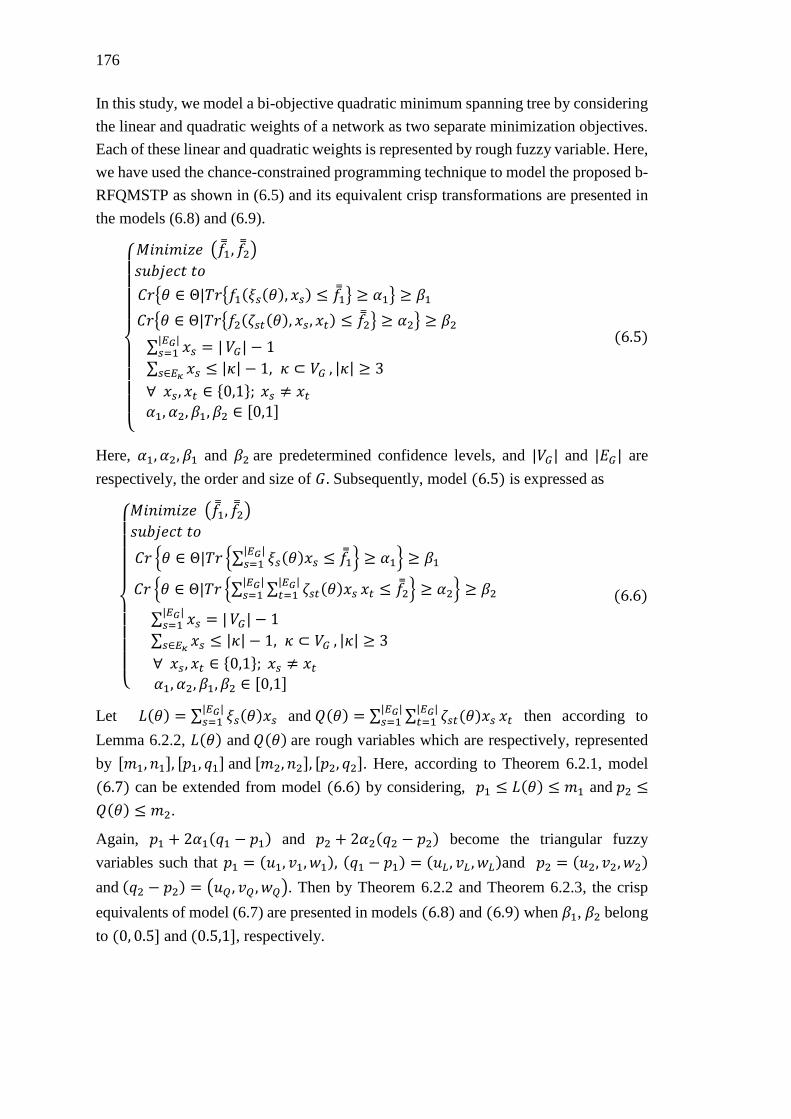
176

In this study, we model a bi-objective quadratic minimum spanning tree by considering

the linear and quadratic weights of a network as two separate minimization objectives.

Each of these linear and quadratic weights is represented by rough fuzzy variable. Here,

we have used the chance-constrained programming technique to model the proposed b-

RFQMSTP as shown in (6.5) and its equivalent crisp transformations are presented in

the models (6.8) and (6.9).

{

𝑀𝑖𝑛𝑖𝑚𝑖𝑧𝑒 (𝑓1, 𝑓2)


𝐶𝑟{휃 ∈ Θ|𝑇𝑟{𝑓1(𝜉𝑠(휃), 𝑥𝑠) ≤ 𝑓1} ≥ 𝛼1} ≥ 𝛽1

𝐶𝑟{휃 ∈ Θ|𝑇𝑟{𝑓2(휁𝑠𝑡(휃), 𝑥𝑠, 𝑥𝑡) ≤ 𝑓2} ≥ 𝛼2} ≥ 𝛽2

∑ 𝑥𝑠 = ||𝐸𝐺|𝑠=1 𝑉𝐺| − 1

∑ 𝑥𝑠 ≤ |𝜅| − 1, 𝜅 ⊂ 𝑉𝐺𝑠∈𝐸𝜅 , |𝜅| ≥ 3

∀ 𝑥𝑠, 𝑥𝑡 ∈ {0,1}; 𝑥𝑠 ≠ 𝑥𝑡

𝛼1, 𝛼2, 𝛽1, 𝛽2 ∈ [0,1]

(6.5)

Here, 𝛼1, 𝛼2, 𝛽1 and 𝛽2 are predetermined confidence levels, and |𝑉𝐺| and |𝐸𝐺| are

respectively, the order and size of 𝐺. Subsequently, model (6.5) is expressed as

{



𝐶𝑟 {휃 ∈ Θ|𝑇𝑟 {∑ 𝜉𝑠(휃)𝑥𝑠|𝐸𝐺|𝑠=1 ≤ 𝑓1} ≥ 𝛼1} ≥ 𝛽1

𝐶𝑟 {휃 ∈ Θ|𝑇𝑟 {∑ ∑ 휁𝑠𝑡(휃)𝑥𝑠|𝐸𝐺|𝑡=1

|𝐸𝐺|𝑠=1 𝑥𝑡 ≤ 𝑓2} ≥ 𝛼2} ≥ 𝛽2

∑ 𝑥𝑠 = ||𝐸𝐺|𝑠=1 𝑉𝐺| − 1

∑ 𝑥𝑠 ≤ |𝜅| − 1, 𝜅 ⊂ 𝑉𝐺𝑠∈𝐸𝜅 , |𝜅| ≥ 3

∀ 𝑥𝑠, 𝑥𝑡 ∈ {0,1}; 𝑥𝑠 ≠ 𝑥𝑡

𝛼1, 𝛼2, 𝛽1, 𝛽2 ∈ [0,1]

(6.6)

Let 𝐿(휃) = ∑ 𝜉𝑠(휃)𝑥𝑠|𝐸𝐺|𝑠=1 and 𝑄(휃) = ∑ ∑ 휁𝑠𝑡(휃)𝑥𝑠

|𝐸𝐺|𝑡=1

|𝐸𝐺|𝑠=1 𝑥𝑡 then according to

Lemma 6.2.2, 𝐿(휃) and 𝑄(휃) are rough variables which are respectively, represented

by [𝑚1, 𝑛1], [𝑝1, 𝑞1] and [𝑚2, 𝑛2], [𝑝2, 𝑞2]. Here, according to Theorem 6.2.1, model

(6.7) can be extended from model (6.6) by considering, 𝑝1 ≤ 𝐿(휃) ≤ 𝑚1 and 𝑝2 ≤

𝑄(휃) ≤ 𝑚2.

Again, 𝑝1 + 2𝛼1(𝑞1 − 𝑝1) and 𝑝2 + 2𝛼2(𝑞2 − 𝑝2) become the triangular fuzzy

variables such that 𝑝1 = (𝑢1, 𝑣1, 𝑤1), (𝑞1 − 𝑝1) = (𝑢𝐿 , 𝑣𝐿 , 𝑤𝐿)and 𝑝2 = (𝑢2, 𝑣2, 𝑤2)

and (𝑞2 − 𝑝2) = (𝑢𝑄 , 𝑣𝑄 , 𝑤𝑄). Then by Theorem 6.2.2 and Theorem 6.2.3, the crisp

equivalents of model (6.7) are presented in models (6.8) and (6.9) when 𝛽1, 𝛽2 belong

to (0, 0.5] and (0.5,1], respectively.

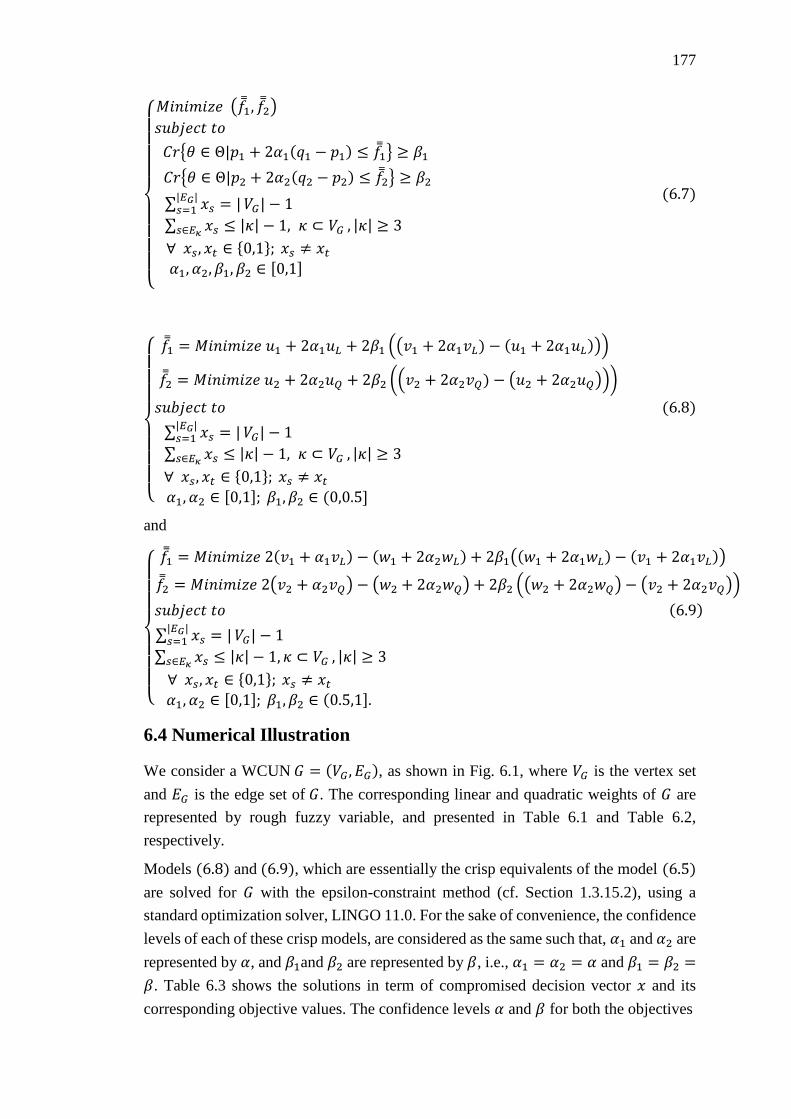
177

{



𝐶𝑟{휃 ∈ Θ|𝑝1 + 2𝛼1(𝑞1 − 𝑝1) ≤ 𝑓1} ≥ 𝛽1

𝐶𝑟{휃 ∈ Θ|𝑝2 + 2𝛼2(𝑞2 − 𝑝2) ≤ 𝑓2} ≥ 𝛽2

∑ 𝑥𝑠 = ||𝐸𝐺|𝑠=1 𝑉𝐺| − 1

∑ 𝑥𝑠 ≤ |𝜅| − 1, 𝜅 ⊂ 𝑉𝐺𝑠∈𝐸𝜅 , |𝜅| ≥ 3

∀ 𝑥𝑠, 𝑥𝑡 ∈ {0,1}; 𝑥𝑠 ≠ 𝑥𝑡

𝛼1, 𝛼2, 𝛽1, 𝛽2 ∈ [0,1]

(6.7)

{

𝑓1 = 𝑀𝑖𝑛𝑖𝑚𝑖𝑧𝑒 𝑢1 + 2𝛼1𝑢𝐿 + 2𝛽1 ((𝑣1 + 2𝛼1𝑣𝐿) − (𝑢1 + 2𝛼1𝑢𝐿)))

𝑓2 = 𝑀𝑖𝑛𝑖𝑚𝑖𝑧𝑒 𝑢2 + 2𝛼2𝑢𝑄 + 2𝛽2 ((𝑣2 + 2𝛼2𝑣𝑄) − (𝑢2 + 2𝛼2𝑢𝑄)))


∑ 𝑥𝑠 = ||𝐸𝐺|𝑠=1 𝑉𝐺| − 1

∑ 𝑥𝑠 ≤ |𝜅| − 1, 𝜅 ⊂ 𝑉𝐺𝑠∈𝐸𝜅 , |𝜅| ≥ 3

∀ 𝑥𝑠, 𝑥𝑡 ∈ {0,1}; 𝑥𝑠 ≠ 𝑥𝑡

𝛼1, 𝛼2 ∈ [0,1]; 𝛽1, 𝛽2 ∈ (0,0.5]

and

{

𝑓1 = 𝑀𝑖𝑛𝑖𝑚𝑖𝑧𝑒 2

(𝑣1 + 𝛼1𝑣𝐿) − (𝑤1 + 2𝛼2𝑤𝐿) + 2𝛽1((𝑤1 + 2𝛼1𝑤𝐿) − (𝑣1 + 2𝛼1𝑣𝐿))

𝑓2 = 𝑀𝑖𝑛𝑖𝑚𝑖𝑧𝑒 2(𝑣2 + 𝛼2𝑣𝑄) − (𝑤2 + 2𝛼2𝑤𝑄) + 2𝛽2 ((𝑤2 + 2𝛼2𝑤𝑄) − (𝑣2 + 2𝛼2𝑣𝑄))


∑ 𝑥𝑠 = ||𝐸𝐺|𝑠=1 𝑉𝐺| − 1

∑ 𝑥𝑠 ≤ |𝜅| − 1, 𝜅 ⊂ 𝑉𝐺𝑠∈𝐸𝜅 , |𝜅| ≥ 3

∀ 𝑥𝑠, 𝑥𝑡 ∈ {0,1}; 𝑥𝑠 ≠ 𝑥𝑡

𝛼1, 𝛼2 ∈ [0,1]; 𝛽1, 𝛽2 ∈ (0.5,1].

6.4 Numerical Illustration

We consider a WCUN 𝐺 = (𝑉𝐺 , 𝐸𝐺), as shown in Fig. 6.1, where 𝑉𝐺 is the vertex set

and 𝐸𝐺 is the edge set of 𝐺. The corresponding linear and quadratic weights of 𝐺 are

represented by rough fuzzy variable, and presented in Table 6.1 and Table 6.2,

respectively.

Models (6.8) and (6.9), which are essentially the crisp equivalents of the model (6.5)

are solved for 𝐺 with the epsilon-constraint method (cf. Section 1.3.15.2), using a

standard optimization solver, LINGO 11.0. For the sake of convenience, the confidence

levels of each of these crisp models, are considered as the same such that, 𝛼1 and 𝛼2 are

represented by 𝛼, and 𝛽1and 𝛽2 are represented by 𝛽, i.e., 𝛼1 = 𝛼2 = 𝛼 and 𝛽1 = 𝛽2 =

𝛽. Table 6.3 shows the solutions in term of compromised decision vector 𝑥 and its

corresponding objective values. The confidence levels 𝛼 and 𝛽 for both the objectives

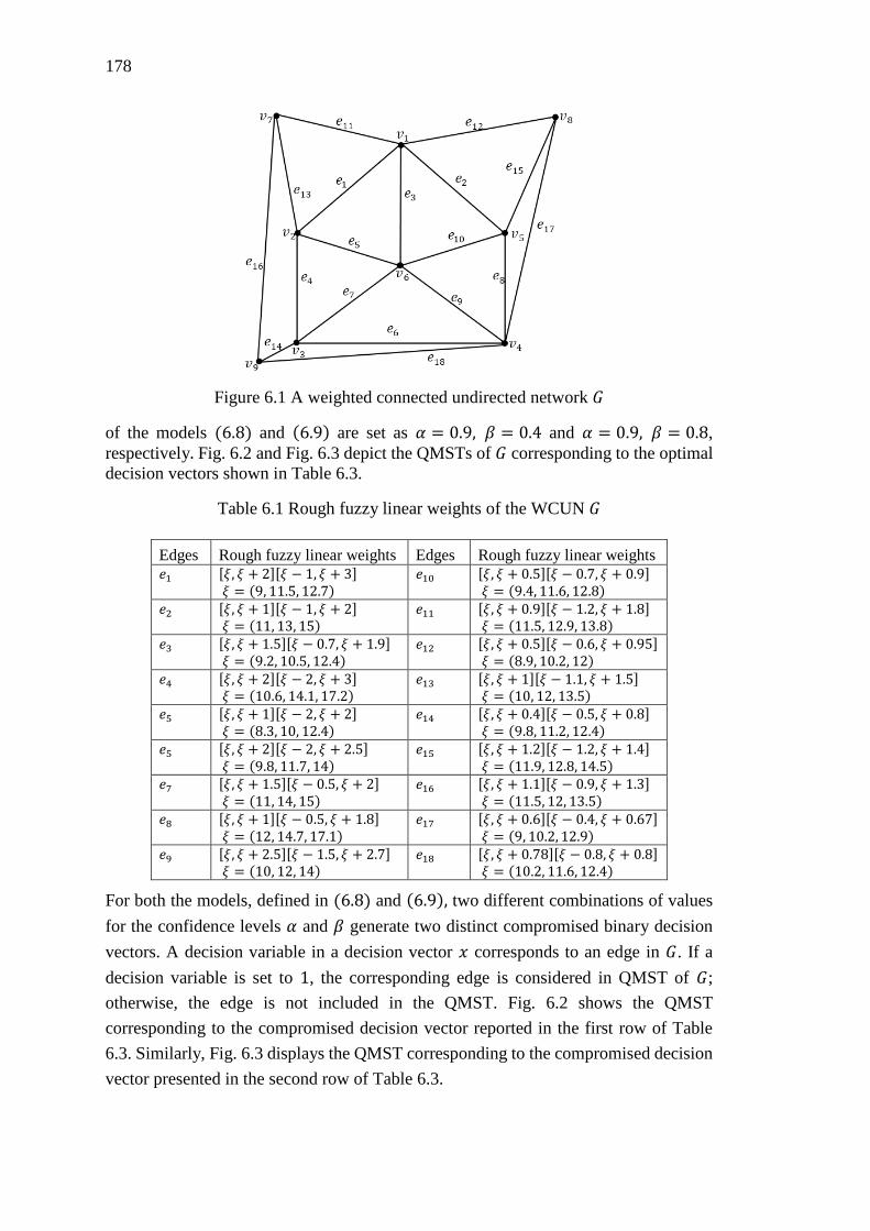
178

Figure 6.1 A weighted connected undirected network 𝐺

of the models (6.8) and (6.9) are set as 𝛼 = 0.9, 𝛽 = 0.4 and 𝛼 = 0.9, 𝛽 = 0.8,

respectively. Fig. 6.2 and Fig. 6.3 depict the QMSTs of 𝐺 corresponding to the optimal

decision vectors shown in Table 6.3.

Table 6.1 Rough fuzzy linear weights of the WCUN 𝐺

For both the models, defined in (6.8) and (6.9), two different combinations of values

for the confidence levels 𝛼 and 𝛽 generate two distinct compromised binary decision

vectors. A decision variable in a decision vector 𝑥 corresponds to an edge in 𝐺. If a

decision variable is set to 1, the corresponding edge is considered in QMST of 𝐺;

otherwise, the edge is not included in the QMST. Fig. 6.2 shows the QMST

corresponding to the compromised decision vector reported in the first row of Table

6.3. Similarly, Fig. 6.3 displays the QMST corresponding to the compromised decision

vector presented in the second row of Table 6.3.

Edges Rough fuzzy linear weights Edges Rough fuzzy linear weights

𝑒1 [𝜉, 𝜉 + 2][𝜉 − 1, 𝜉 + 3] 𝜉 = (9, 11.5, 12.7)

𝑒10 [𝜉, 𝜉 + 0.5][𝜉 − 0.7, 𝜉 + 0.9] 𝜉 = (9.4, 11.6, 12.8)

𝑒2 [𝜉, 𝜉 + 1][𝜉 − 1, 𝜉 + 2] 𝜉 = (11, 13, 15)

𝑒11 [𝜉, 𝜉 + 0.9][𝜉 − 1.2, 𝜉 + 1.8] 𝜉 = (11.5, 12.9, 13.8)

𝑒3 [𝜉, 𝜉 + 1.5][𝜉 − 0.7, 𝜉 + 1.9] 𝜉 = (9.2, 10.5, 12.4)

𝑒12 [𝜉, 𝜉 + 0.5][𝜉 − 0.6, 𝜉 + 0.95] 𝜉 = (8.9, 10.2, 12)

𝑒4 [𝜉, 𝜉 + 2][𝜉 − 2, 𝜉 + 3] 𝜉 = (10.6, 14.1, 17.2)

𝑒13 [𝜉, 𝜉 + 1][𝜉 − 1.1, 𝜉 + 1.5] 𝜉 = (10, 12, 13.5)

𝑒5 [𝜉, 𝜉 + 1][𝜉 − 2, 𝜉 + 2] 𝜉 = (8.3, 10, 12.4)

𝑒14 [𝜉, 𝜉 + 0.4][𝜉 − 0.5, 𝜉 + 0.8] 𝜉 = (9.8, 11.2, 12.4)

𝑒5 [𝜉, 𝜉 + 2][𝜉 − 2, 𝜉 + 2.5] 𝜉 = (9.8, 11.7, 14)

𝑒15 [𝜉, 𝜉 + 1.2][𝜉 − 1.2, 𝜉 + 1.4] 𝜉 = (11.9, 12.8, 14.5)

𝑒7 [𝜉, 𝜉 + 1.5][𝜉 − 0.5, 𝜉 + 2] 𝜉 = (11, 14, 15)

𝑒16 [𝜉, 𝜉 + 1.1][𝜉 − 0.9, 𝜉 + 1.3] 𝜉 = (11.5, 12, 13.5)

𝑒8 [𝜉, 𝜉 + 1][𝜉 − 0.5, 𝜉 + 1.8] 𝜉 = (12, 14.7, 17.1)

𝑒17 [𝜉, 𝜉 + 0.6][𝜉 − 0.4, 𝜉 + 0.67] 𝜉 = (9, 10.2, 12.9)

𝑒9 [𝜉, 𝜉 + 2.5][𝜉 − 1.5, 𝜉 + 2.7] 𝜉 = (10, 12, 14)

𝑒18 [𝜉, 𝜉 + 0.78][𝜉 − 0.8, 𝜉 + 0.8] 𝜉 = (10.2, 11.6, 12.4)

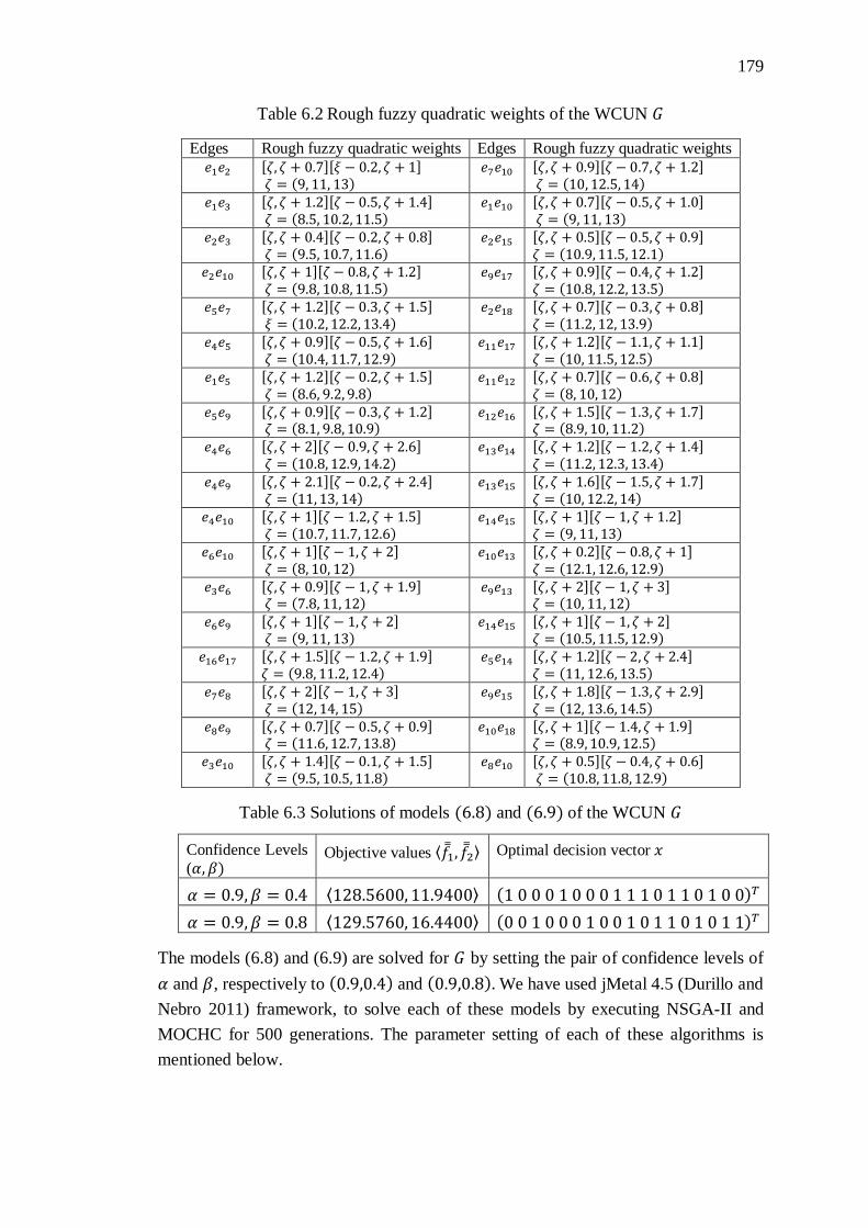
179

Table 6.2 Rough fuzzy quadratic weights of the WCUN 𝐺

Edges Rough fuzzy quadratic weights Edges Rough fuzzy quadratic weights

𝑒1𝑒2 [휁, 휁 + 0.7][𝜉 − 0.2, 휁 + 1] 휁 = (9, 11, 13)

𝑒7𝑒10 [휁, 휁 + 0.9][휁 − 0.7, 휁 + 1.2] 휁 = (10, 12.5, 14)

𝑒1𝑒3 [휁, 휁 + 1.2][휁 − 0.5, 휁 + 1.4] 휁 = (8.5, 10.2, 11.5)

𝑒1𝑒10 [휁, 휁 + 0.7][휁 − 0.5, 휁 + 1.0] 휁 = (9, 11, 13)

𝑒2𝑒3 [휁, 휁 + 0.4][휁 − 0.2, 휁 + 0.8] 휁 = (9.5, 10.7, 11.6)

𝑒2𝑒15 [휁, 휁 + 0.5][휁 − 0.5, 휁 + 0.9] 휁 = (10.9, 11.5, 12.1)

𝑒2𝑒10 [휁, 휁 + 1][휁 − 0.8, 휁 + 1.2] 휁 = (9.8, 10.8, 11.5)

𝑒9𝑒17 [휁, 휁 + 0.9][휁 − 0.4, 휁 + 1.2] 휁 = (10.8, 12.2, 13.5)

𝑒5𝑒7 [휁, 휁 + 1.2][휁 − 0.3, 휁 + 1.5] 𝜉 = (10.2, 12.2, 13.4)

𝑒2𝑒18 [휁, 휁 + 0.7][휁 − 0.3, 휁 + 0.8] 휁 = (11.2, 12, 13.9)

𝑒4𝑒5 [휁, 휁 + 0.9][휁 − 0.5, 휁 + 1.6] 휁 = (10.4, 11.7, 12.9)

𝑒11𝑒17 [휁, 휁 + 1.2][휁 − 1.1, 휁 + 1.1] 휁 = (10, 11.5, 12.5)

𝑒1𝑒5 [휁, 휁 + 1.2][휁 − 0.2, 휁 + 1.5] 휁 = (8.6, 9.2, 9.8)

𝑒11𝑒12 [휁, 휁 + 0.7][휁 − 0.6, 휁 + 0.8] 휁 = (8, 10, 12)

𝑒5𝑒9 [휁, 휁 + 0.9][휁 − 0.3, 휁 + 1.2] 휁 = (8.1, 9.8, 10.9)

𝑒12𝑒16 [휁, 휁 + 1.5][휁 − 1.3, 휁 + 1.7] 휁 = (8.9, 10, 11.2)

𝑒4𝑒6 [휁, 휁 + 2][휁 − 0.9, 휁 + 2.6] 휁 = (10.8, 12.9, 14.2)

𝑒13𝑒14 [휁, 휁 + 1.2][휁 − 1.2, 휁 + 1.4] 휁 = (11.2, 12.3, 13.4)

𝑒4𝑒9 [휁, 휁 + 2.1][휁 − 0.2, 휁 + 2.4] 휁 = (11, 13, 14)

𝑒13𝑒15 [휁, 휁 + 1.6][휁 − 1.5, 휁 + 1.7] 휁 = (10, 12.2, 14)

𝑒4𝑒10 [휁, 휁 + 1][휁 − 1.2, 휁 + 1.5] 휁 = (10.7, 11.7, 12.6)

𝑒14𝑒15 [휁, 휁 + 1][휁 − 1, 휁 + 1.2] 휁 = (9, 11, 13)

𝑒6𝑒10 [휁, 휁 + 1][휁 − 1, 휁 + 2] 휁 = (8, 10, 12)

𝑒10𝑒13 [휁, 휁 + 0.2][휁 − 0.8, 휁 + 1] 휁 = (12.1, 12.6, 12.9)

𝑒3𝑒6 [휁, 휁 + 0.9][휁 − 1, 휁 + 1.9] 휁 = (7.8, 11, 12)

𝑒9𝑒13 [휁, 휁 + 2][휁 − 1, 휁 + 3] 휁 = (10, 11, 12)

𝑒6𝑒9 [휁, 휁 + 1][휁 − 1, 휁 + 2] 휁 = (9, 11, 13)

𝑒14𝑒15 [휁, 휁 + 1][휁 − 1, 휁 + 2] 휁 = (10.5, 11.5, 12.9)

𝑒16𝑒17 [휁, 휁 + 1.5][휁 − 1.2, 휁 + 1.9] 휁 = (9.8, 11.2, 12.4)

𝑒5𝑒14 [휁, 휁 + 1.2][휁 − 2, 휁 + 2.4] 휁 = (11, 12.6, 13.5)

𝑒7𝑒8 [휁, 휁 + 2][휁 − 1, 휁 + 3] 휁 = (12, 14, 15)

𝑒9𝑒15 [휁, 휁 + 1.8][휁 − 1.3, 휁 + 2.9] 휁 = (12, 13.6, 14.5)

𝑒8𝑒9 [휁, 휁 + 0.7][휁 − 0.5, 휁 + 0.9] 휁 = (11.6, 12.7, 13.8)

𝑒10𝑒18 [휁, 휁 + 1][휁 − 1.4, 휁 + 1.9] 휁 = (8.9, 10.9, 12.5)

𝑒3𝑒10 [휁, 휁 + 1.4][휁 − 0.1, 휁 + 1.5] 휁 = (9.5, 10.5, 11.8)

𝑒8𝑒10 [휁, 휁 + 0.5][휁 − 0.4, 휁 + 0.6] 휁 = (10.8, 11.8, 12.9)

Table 6.3 Solutions of models (6.8) and (6.9) of the WCUN 𝐺

Confidence Levels

(𝛼, 𝛽) Objective values ⟨𝑓1, 𝑓2⟩ Optimal decision vector 𝑥

𝛼 = 0.9, 𝛽 = 0.4 ⟨128.5600, 11.9400⟩ (1 0 0 0 1 0 0 0 1 1 1 0 1 1 0 1 0 0)𝑇

𝛼 = 0.9, 𝛽 = 0.8 ⟨129.5760, 16.4400⟩ (0 0 1 0 0 0 1 0 0 1 0 1 1 0 1 0 1 1)𝑇

The models (6.8) and (6.9) are solved for 𝐺 by setting the pair of confidence levels of

𝛼 and 𝛽, respectively to (0.9,0.4) and (0.9,0.8). We have used jMetal 4.5 (Durillo and

Nebro 2011) framework, to solve each of these models by executing NSGA-II and

MOCHC for 500 generations. The parameter setting of each of these algorithms is

mentioned below.

180

Figure 6.2 A rough fuzzy quadratic minimum spanning tree of the WCUN 𝐺 with 𝛼 =0.9 and 𝛽 = 0.4

Figure 6.3 A rough fuzzy quadratic minimum spanning tree of the WCUN 𝐺 with 𝛼 =0.9 and 𝛽 = 0.8

The nondominated solutions of the model (6.8) are displayed in Fig. 6.4 (a) and Fig.

6.4 (b), and that of the model (6.9) are shown in Fig. 6.5 (a) and Fig. 6.5 (b).

Specifically, the nondominated solutions generated by NSGA-II are displayed in Fig.

6.4 (a) and Fig. 6.5 (a). Whereas, Fig. 6.4 (b) and Fig. 6.5 (b) depict the nondominated

solutions generated by MOCHC. The solutions generated by the epsilon-constraint

method at different confidence levels are also shown in each of these figures, which are

also nondominated as compared to the solutions of NSGA-II and MOCHC.

For NSGA-II: Population size = 100, maximum generations = 500, crossover

probability = 0.9, mutation probability = 0.03.

For MOCHC: Population size = 100, maximum generations = 500, crossover

probability = 0.9, incest threshold count = 0.25, convergence value = 1, preserved

population = 0.05.

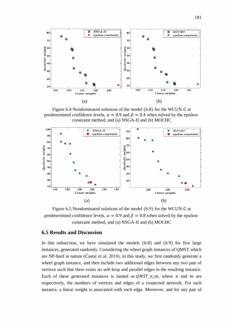
181

(a) (b)



constraint method, and (a) NSGA-II and (b) MOCHC

(a) (b)





In this subsection, we have simulated the models (6.8) and (6.9) for five large

instances, generated randomly. Considering the wheel graph instances of QMST which

are NP-hard in nature (Ćustić et al. 2018), in this study, we first randomly generate a

wheel graph instance, and then include two additional edges between any two pair of

vertices such that there exists no self-loop and parallel edges in the resulting instance.

Each of these generated instances is named as 𝑄𝑀𝑆𝑇_𝑛_𝑚, where 𝑛 and 𝑚 are

respectively, the numbers of vertices and edges of a connected network. For each

instance, a linear weight is associated with each edge. Moreover, and for any pair of

182

edges, there exists a quadratic weight. The linear and quadratic weights are generated

randomly and represented by rough fuzzy variable. While simulating model (6.8) for

each those five instances, the confidence levels 𝛼 and 𝛽 are respectively, set to

0.9 and 0.4. Whereas, when the model (6.9) is considered, 𝛼 and 𝛽 are respectively, set

to 0.9 and 0.8. Subsequently, the random instances are solved with two MOGAs:

NSGA-II and MOCHC. Moreover, the corresponding performance metrics, e.g.,

hypervolume (𝐻𝑉) (Zitzler and Thiele 1999), spread (Δ) (Zhou et al. 2006),

generational distance (𝐺𝐷) (Van Veldhuizen and Lamont 1998) and inverted

generational distance (𝐼𝐺𝐷) (Van Veldhuizen and Lamont 1998) are studied to make a

comparison between the MOGAs. For any MOGA, larger values of 𝐻𝑉 and smaller

values of Δ, 𝐺𝐷 and 𝐼𝐺𝐷 are desirable. Moreover, for a particular MOGA, each of these

performance metrics determines either the convergence or the diversity or the both.

Particularly, the 𝐻𝑉 and the 𝐼𝐺𝐷 metrics are used to measure both the convergence and

diversity among the solutions. Furthermore, the diversity and the convergence among

the solutions are measured by Δ and 𝐺𝐷, respectively.

We have used jMetal 4.5 for the simulation of the two MOGAs: NSGA-II and MOCHC,

for the instances. As the algorithms are stochastic in nature, we execute each of them

for 100 times by considering 500 generations for each execution. Since there does not

exist Pareto optimal solutions of any rough fuzzy bi-objective quadratic minimum

spanning problem in the literature, therefore, we approximate the Pareto front of each

of the instances by collecting their best solutions obtained from the first font of NSGA-

II and MOCHC. The parameter settings for NSGA-II and MOCHC are considered the

same as mentioned above in Section 6.4.

Subsequently, some statistical measures of the performance metrics are studied which

are reported in Table 6.4 through Table 6.7, where the better values are highlighted as

bold. Specifically, for all the performance metrics, the 𝑚𝑒𝑎𝑛 and the standard deviation

(𝑠𝑑) are shown in Table 6.4 and Table 6.6, whereas, the 𝑚𝑒𝑑𝑖𝑎𝑛 and the interquartile

range (𝐼𝑄𝑅) are reported in Table 6.5 and Table 6.7. Considering Table 6.4, MOCHC

performs better than NSGA-II for all the five instances with respect to Δ. Moreover,

MOCHC becomes superior to NSGA-II relating to 𝐺𝐷 and 𝐼𝐺𝐷, respectively for four

and three instances. However, for 𝐻𝑉, NSGA-II performs better than MOCHC,

respectively for three instances. Similar to Table 6.4, in Table 6.5, MOCHC performs

better than NSGA-II for all the instances as far as Δ is concerned. For 𝐺𝐷 and 𝐼𝐺𝐷,

MOCHC becomes superior to NSGA-II for three out of five instances. However,

considering 𝐻𝑉, NSGA-II performs better than MOCHC for three instances. Therefore,

for most of the instances, in tables 6.4 and 6.5, we observe that MOCHC is superior to

NSGA-II with respect to Δ, 𝐺𝐷 and 𝐼𝐺𝐷, and NSGA-II becomes superior to MOCHC

with respect to 𝐻𝑉.

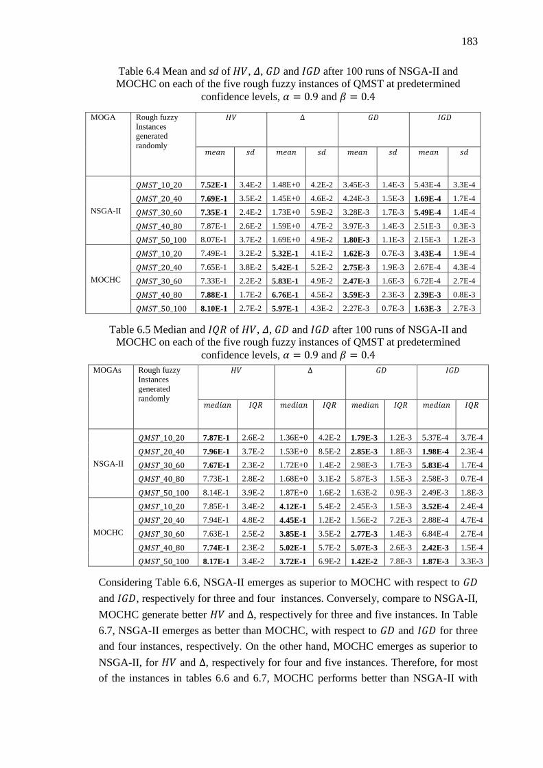
183

Table 6.4 Mean and sd of 𝐻𝑉, 𝛥, 𝐺𝐷 and 𝐼𝐺𝐷 after 100 runs of NSGA-II and


confidence levels, 𝛼 = 0.9 and 𝛽 = 0.4

MOGA Rough fuzzy

Instances

generated

randomly

𝐻𝑉 Δ 𝐺𝐷 𝐼𝐺𝐷

𝑚𝑒𝑎𝑛 𝑠𝑑 𝑚𝑒𝑎𝑛 𝑠𝑑 𝑚𝑒𝑎𝑛 𝑠𝑑 𝑚𝑒𝑎𝑛 𝑠𝑑

NSGA-II

𝑄𝑀𝑆𝑇_10_20 7.52E-1 3.4E-2 1.48E+0 4.2E-2 3.45E-3 1.4E-3 5.43E-4 3.3E-4

𝑄𝑀𝑆𝑇_20_40 7.69E-1 3.5E-2 1.45E+0 4.6E-2 4.24E-3 1.5E-3 1.69E-4 1.7E-4

𝑄𝑀𝑆𝑇_30_60 7.35E-1 2.4E-2 1.73E+0 5.9E-2 3.28E-3 1.7E-3 5.49E-4 1.4E-4

𝑄𝑀𝑆𝑇_40_80 7.87E-1 2.6E-2 1.59E+0 4.7E-2 3.97E-3 1.4E-3 2.51E-3 0.3E-3

𝑄𝑀𝑆𝑇_50_100 8.07E-1 3.7E-2 1.69E+0 4.9E-2 1.80E-3 1.1E-3 2.15E-3 1.2E-3

MOCHC

𝑄𝑀𝑆𝑇_10_20 7.49E-1 3.2E-2 5.32E-1 4.1E-2 1.62E-3 0.7E-3 3.43E-4 1.9E-4

𝑄𝑀𝑆𝑇_20_40 7.65E-1 3.8E-2 5.42E-1 5.2E-2 2.75E-3 1.9E-3 2.67E-4 4.3E-4

𝑄𝑀𝑆𝑇_30_60 7.33E-1 2.2E-2 5.83E-1 4.9E-2 2.47E-3 1.6E-3 6.72E-4 2.7E-4

𝑄𝑀𝑆𝑇_40_80 7.88E-1 1.7E-2 6.76E-1 4.5E-2 3.59E-3 2.3E-3 2.39E-3 0.8E-3

𝑄𝑀𝑆𝑇_50_100 8.10E-1 2.7E-2 5.97E-1 4.3E-2 2.27E-3 0.7E-3 1.63E-3 2.7E-3

Table 6.5 Median and 𝐼𝑄𝑅 of 𝐻𝑉, 𝛥, 𝐺𝐷 and 𝐼𝐺𝐷 after 100 runs of NSGA-II and



MOGAs Rough fuzzy

Instances

generated

randomly


𝑚𝑒𝑑𝑖𝑎𝑛 𝐼𝑄𝑅 𝑚𝑒𝑑𝑖𝑎𝑛 𝐼𝑄𝑅 𝑚𝑒𝑑𝑖𝑎𝑛 𝐼𝑄𝑅 𝑚𝑒𝑑𝑖𝑎𝑛 𝐼𝑄𝑅

NSGA-II

𝑄𝑀𝑆𝑇_10_20 7.87E-1 2.6E-2 1.36E+0 4.2E-2 1.79E-3 1.2E-3 5.37E-4 3.7E-4

𝑄𝑀𝑆𝑇_20_40 7.96E-1 3.7E-2 1.53E+0 8.5E-2 2.85E-3 1.8E-3 1.98E-4 2.3E-4

𝑄𝑀𝑆𝑇_30_60 7.67E-1 2.3E-2 1.72E+0 1.4E-2 2.98E-3 1.7E-3 5.83E-4 1.7E-4

𝑄𝑀𝑆𝑇_40_80 7.73E-1 2.8E-2 1.68E+0 3.1E-2 5.87E-3 1.5E-3 2.58E-3 0.7E-4

𝑄𝑀𝑆𝑇_50_100 8.14E-1 3.9E-2 1.87E+0 1.6E-2 1.63E-2 0.9E-3 2.49E-3 1.8E-3

MOCHC

𝑄𝑀𝑆𝑇_10_20 7.85E-1 3.4E-2 4.12E-1 5.4E-2 2.45E-3 1.5E-3 3.52E-4 2.4E-4

𝑄𝑀𝑆𝑇_20_40 7.94E-1 4.8E-2 4.45E-1 1.2E-2 1.56E-2 7.2E-3 2.88E-4 4.7E-4

𝑄𝑀𝑆𝑇_30_60 7.63E-1 2.5E-2 3.85E-1 3.5E-2 2.77E-3 1.4E-3 6.84E-4 2.7E-4

𝑄𝑀𝑆𝑇_40_80 7.74E-1 2.3E-2 5.02E-1 5.7E-2 5.07E-3 2.6E-3 2.42E-3 1.5E-4

𝑄𝑀𝑆𝑇_50_100 8.17E-1 3.4E-2 3.72E-1 6.9E-2 1.42E-2 7.8E-3 1.87E-3 3.3E-3

Considering Table 6.6, NSGA-II emerges as superior to MOCHC with respect to 𝐺𝐷

and 𝐼𝐺𝐷, respectively for three and four instances. Conversely, compare to NSGA-II,

MOCHC generate better 𝐻𝑉 and Δ, respectively for three and five instances. In Table

6.7, NSGA-II emerges as better than MOCHC, with respect to 𝐺𝐷 and 𝐼𝐺𝐷 for three

and four instances, respectively. On the other hand, MOCHC emerges as superior to

NSGA-II, for 𝐻𝑉 and Δ, respectively for four and five instances. Therefore, for most

of the instances in tables 6.6 and 6.7, MOCHC performs better than NSGA-II with

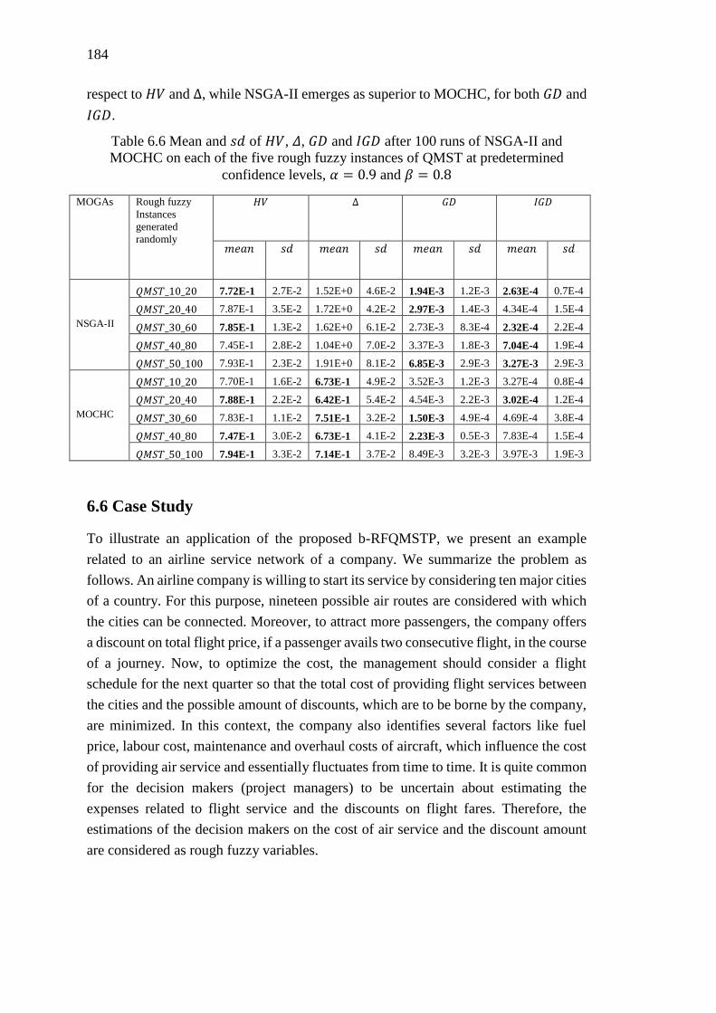
184

respect to 𝐻𝑉 and Δ, while NSGA-II emerges as superior to MOCHC, for both 𝐺𝐷 and

𝐼𝐺𝐷.

Table 6.6 Mean and 𝑠𝑑 of 𝐻𝑉, 𝛥, 𝐺𝐷 and 𝐼𝐺𝐷 after 100 runs of NSGA-II and



MOGAs Rough fuzzy

Instances

generated

randomly


𝑚𝑒𝑎𝑛 𝑠𝑑 𝑚𝑒𝑎𝑛 𝑠𝑑 𝑚𝑒𝑎𝑛 𝑠𝑑 𝑚𝑒𝑎𝑛 𝑠𝑑

NSGA-II

𝑄𝑀𝑆𝑇_10_20 7.72E-1 2.7E-2 1.52E+0 4.6E-2 1.94E-3 1.2E-3 2.63E-4 0.7E-4

𝑄𝑀𝑆𝑇_20_40 7.87E-1 3.5E-2 1.72E+0 4.2E-2 2.97E-3 1.4E-3 4.34E-4 1.5E-4

𝑄𝑀𝑆𝑇_30_60 7.85E-1 1.3E-2 1.62E+0 6.1E-2 2.73E-3 8.3E-4 2.32E-4 2.2E-4

𝑄𝑀𝑆𝑇_40_80 7.45E-1 2.8E-2 1.04E+0 7.0E-2 3.37E-3 1.8E-3 7.04E-4 1.9E-4

𝑄𝑀𝑆𝑇_50_100 7.93E-1 2.3E-2 1.91E+0 8.1E-2 6.85E-3 2.9E-3 3.27E-3 2.9E-3

MOCHC

𝑄𝑀𝑆𝑇_10_20 7.70E-1 1.6E-2 6.73E-1 4.9E-2 3.52E-3 1.2E-3 3.27E-4 0.8E-4

𝑄𝑀𝑆𝑇_20_40 7.88E-1 2.2E-2 6.42E-1 5.4E-2 4.54E-3 2.2E-3 3.02E-4 1.2E-4

𝑄𝑀𝑆𝑇_30_60 7.83E-1 1.1E-2 7.51E-1 3.2E-2 1.50E-3 4.9E-4 4.69E-4 3.8E-4

𝑄𝑀𝑆𝑇_40_80 7.47E-1 3.0E-2 6.73E-1 4.1E-2 2.23E-3 0.5E-3 7.83E-4 1.5E-4

𝑄𝑀𝑆𝑇_50_100 7.94E-1 3.3E-2 7.14E-1 3.7E-2 8.49E-3 3.2E-3 3.97E-3 1.9E-3

6.6 Case Study

To illustrate an application of the proposed b-RFQMSTP, we present an example

related to an airline service network of a company. We summarize the problem as

follows. An airline company is willing to start its service by considering ten major cities

of a country. For this purpose, nineteen possible air routes are considered with which

the cities can be connected. Moreover, to attract more passengers, the company offers

a discount on total flight price, if a passenger avails two consecutive flight, in the course

of a journey. Now, to optimize the cost, the management should consider a flight

schedule for the next quarter so that the total cost of providing flight services between

the cities and the possible amount of discounts, which are to be borne by the company,

are minimized. In this context, the company also identifies several factors like fuel

price, labour cost, maintenance and overhaul costs of aircraft, which influence the cost

of providing air service and essentially fluctuates from time to time. It is quite common

for the decision makers (project managers) to be uncertain about estimating the

expenses related to flight service and the discounts on flight fares. Therefore, the

estimations of the decision makers on the cost of air service and the discount amount

are considered as rough fuzzy variables.

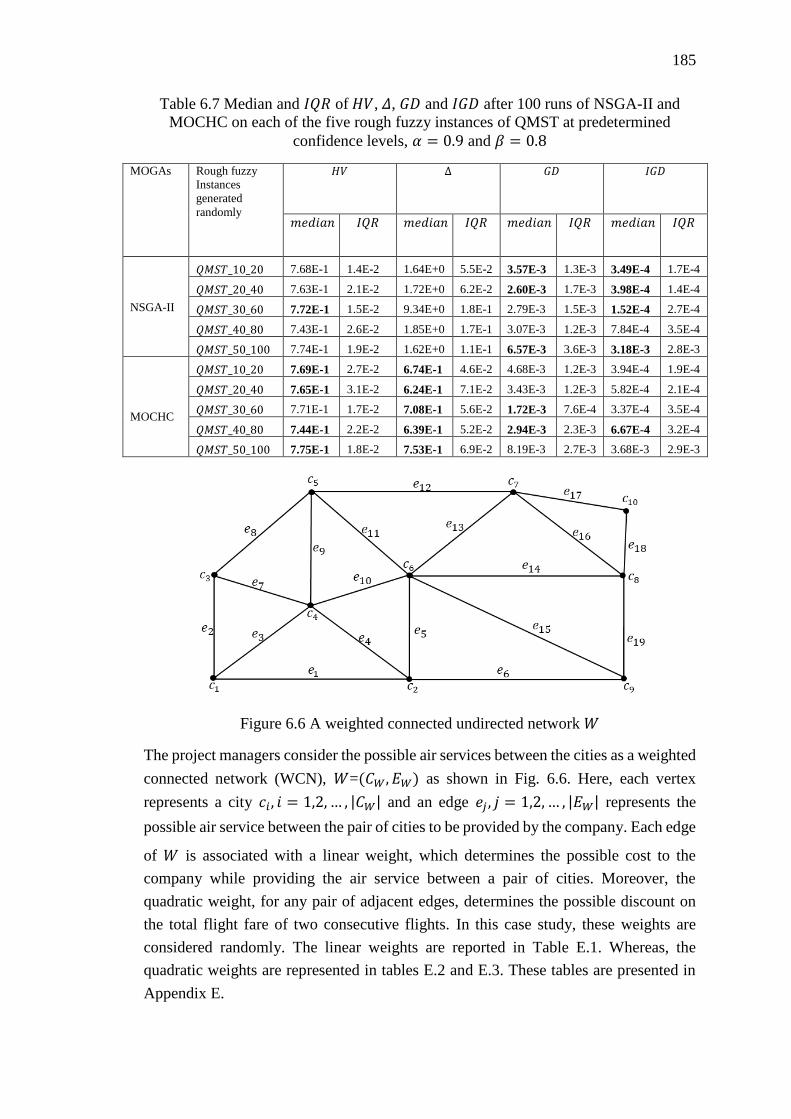
185

Table 6.7 Median and 𝐼𝑄𝑅 of 𝐻𝑉, 𝛥, 𝐺𝐷 and 𝐼𝐺𝐷 after 100 runs of NSGA-II and



MOGAs Rough fuzzy

Instances

generated

randomly


𝑚𝑒𝑑𝑖𝑎𝑛 𝐼𝑄𝑅 𝑚𝑒𝑑𝑖𝑎𝑛 𝐼𝑄𝑅 𝑚𝑒𝑑𝑖𝑎𝑛 𝐼𝑄𝑅 𝑚𝑒𝑑𝑖𝑎𝑛 𝐼𝑄𝑅

NSGA-II

𝑄𝑀𝑆𝑇_10_20 7.68E-1 1.4E-2 1.64E+0 5.5E-2 3.57E-3 1.3E-3 3.49E-4 1.7E-4

𝑄𝑀𝑆𝑇_20_40 7.63E-1 2.1E-2 1.72E+0 6.2E-2 2.60E-3 1.7E-3 3.98E-4 1.4E-4

𝑄𝑀𝑆𝑇_30_60 7.72E-1 1.5E-2 9.34E+0 1.8E-1 2.79E-3 1.5E-3 1.52E-4 2.7E-4

𝑄𝑀𝑆𝑇_40_80 7.43E-1 2.6E-2 1.85E+0 1.7E-1 3.07E-3 1.2E-3 7.84E-4 3.5E-4

𝑄𝑀𝑆𝑇_50_100 7.74E-1 1.9E-2 1.62E+0 1.1E-1 6.57E-3 3.6E-3 3.18E-3 2.8E-3

MOCHC

𝑄𝑀𝑆𝑇_10_20 7.69E-1 2.7E-2 6.74E-1 4.6E-2 4.68E-3 1.2E-3 3.94E-4 1.9E-4

𝑄𝑀𝑆𝑇_20_40 7.65E-1 3.1E-2 6.24E-1 7.1E-2 3.43E-3 1.2E-3 5.82E-4 2.1E-4

𝑄𝑀𝑆𝑇_30_60 7.71E-1 1.7E-2 7.08E-1 5.6E-2 1.72E-3 7.6E-4 3.37E-4 3.5E-4

𝑄𝑀𝑆𝑇_40_80 7.44E-1 2.2E-2 6.39E-1 5.2E-2 2.94E-3 2.3E-3 6.67E-4 3.2E-4

𝑄𝑀𝑆𝑇_50_100 7.75E-1 1.8E-2 7.53E-1 6.9E-2 8.19E-3 2.7E-3 3.68E-3 2.9E-3

Figure 6.6 A weighted connected undirected network 𝑊

The project managers consider the possible air services between the cities as a weighted

connected network (WCN), 𝑊=(𝐶𝑊, 𝐸𝑊) as shown in Fig. 6.6. Here, each vertex

represents a city 𝑐𝑖, 𝑖 = 1,2, … , |𝐶𝑊| and an edge 𝑒𝑗 , 𝑗 = 1,2, … , |𝐸𝑊| represents the

possible air service between the pair of cities to be provided by the company. Each edge

of 𝑊 is associated with a linear weight, which determines the possible cost to the

company while providing the air service between a pair of cities. Moreover, the

quadratic weight, for any pair of adjacent edges, determines the possible discount on

the total flight fare of two consecutive flights. In this case study, these weights are

considered randomly. The linear weights are reported in Table E.1. Whereas, the

quadratic weights are represented in tables E.2 and E.3. These tables are presented in

Appendix E.

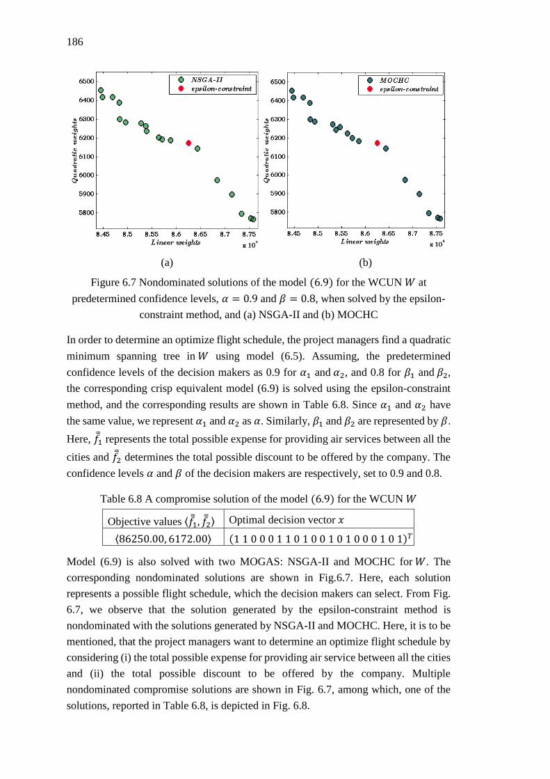
186

(a) (b)

Figure 6.7 Nondominated solutions of the model (6.9) for the WCUN 𝑊 at

predetermined confidence levels, 𝛼 = 0.9 and 𝛽 = 0.8, when solved by the epsilon-


In order to determine an optimize flight schedule, the project managers find a quadratic

minimum spanning tree in 𝑊 using model (6.5). Assuming, the predetermined

confidence levels of the decision makers as 0.9 for 𝛼1 and 𝛼2, and 0.8 for 𝛽1 and 𝛽2,

the corresponding crisp equivalent model (6.9) is solved using the epsilon-constraint

method, and the corresponding results are shown in Table 6.8. Since 𝛼1 and 𝛼2 have

the same value, we represent 𝛼1 and 𝛼2 as 𝛼. Similarly, 𝛽1 and 𝛽2 are represented by 𝛽.

Here, 𝑓1 represents the total possible expense for providing air services between all the

cities and 𝑓2 determines the total possible discount to be offered by the company. The

confidence levels 𝛼 and 𝛽 of the decision makers are respectively, set to 0.9 and 0.8.

Table 6.8 A compromise solution of the model (6.9) for the WCUN 𝑊

Objective values ⟨𝑓1, 𝑓2⟩ Optimal decision vector 𝑥

⟨86250.00, 6172.00⟩ (1 1 0 0 0 1 1 0 1 0 0 1 0 1 0 0 0 1 0 1)𝑇

Model (6.9) is also solved with two MOGAS: NSGA-II and MOCHC for 𝑊. The

corresponding nondominated solutions are shown in Fig.6.7. Here, each solution

represents a possible flight schedule, which the decision makers can select. From Fig.

6.7, we observe that the solution generated by the epsilon-constraint method is

nondominated with the solutions generated by NSGA-II and MOCHC. Here, it is to be

mentioned, that the project managers want to determine an optimize flight schedule by

considering (i) the total possible expense for providing air service between all the cities

and (ii) the total possible discount to be offered by the company. Multiple

nondominated compromise solutions are shown in Fig. 6.7, among which, one of the

solutions, reported in Table 6.8, is depicted in Fig. 6.8.

187

Figure 6.8 A possible flight schedule for the compromise solution of the WCUN 𝑊 as

reported in Table 6.8

6.7 Conclusion

In this chapter, we have proposed a b-RFQMSTP which is modelled using the rough

fuzzy chance-constrained programming technique. The linear and quadratic weights of

the proposed model are considered as two different objectives which are optimized

simultaneously. Till now, any study under such rough fuzzy uncertain environment is

yet to be conducted in the literature, where the associated parameters are essentially

considered as rough fuzzy variables. The crisp equivalent of the proposed model is

solved by the epsilon-constraint method and by two MOGAs: NSGA-II and MOCHC.

For each of the MOGAs, the proposed model is also solved for five randomly generated

rough fuzzy instances, at two different combinations of the confidence levels: (i) 𝛼 =

0.9 and 𝛽 = 0.4 and (ii) 𝛼 = 0.9 and 𝛽 = 0.8. The performance of these MOGAs are

analyzed for all the five instances with respect to four different performance metrics:

(i) 𝐻𝑉, (ii) Δ, (iii) 𝐺𝐷 and (iv) 𝐼𝐺𝐷. Moreover, in this study, we have also presented an

example to numerically illustrate an application of the proposed model.

In future, the rough fuzzy chance-constrained programming model can also be extended

to model different network optimization problems including shortest path, maximum

flow and transportation. Moreover, optimization problems in the domains of portfolio,

inventory, supply chain, etc., can also be addressed using rough fuzzy chance-

constrained programming.

188

User

Text Box

189

Chapter 7

Conclusion and Future Scope

User

Text Box

190

User

Text Box

191

Chapter 7

Conclusion and Future Scope

7.1 Conclusion

In this dissertation, we have proposed two single and three multi-objective network

optimization problems under different uncertain paradigms including type-2 fuzzy,

random fuzzy, rough, rough fuzzy, and uncertainty theory. Those uncertain network

models are formulated using uncertain programming techniques and are solved by

different classical and evolutionary algorithms. The main contribution of this thesis is

presented in five chapters, which are again categorized into two parts. Part-I consists of

Chapter 2 and Chapter 3. While, Part-II contains Chapter 4, Chapter 5 and Chapter 6.

Chapter 1 contains introduction of the thesis, and conclusion and future scope of the

thesis are discussed in Chapter 7. In Chapter 2, we have proposed a linear programming

problem with interval type-2 fuzzy parameters. The formulation of the LPP is based on

chance-constrained programming and credibility measure of IT2FV. The applicability

of the proposed method is demonstrated by solving three network problems: (i) solid

transportation problem (STP), (ii) shortest path problem (SPP) and (iii) minimum

spanning tree problem (MSTP).

The study in Chapter 3 deals with random fuzzy maximum flow problem (MFP), where

we have proposed the corresponding expected value model (EVM) and chance-

constrained model (CCM) of the problem. We have also developed the varying

population genetic algorithm with indeterminate crossover (VPGAwIC) to solve the

crisp equivalent of the MFP. In the proposed algorithm, the selection of a chromosome

depends on its lifetime. For this purpose, in our study, we have also proposed an

improved lifetime allocation strategy (iLAS). The proposed algorithm is compared with

other similar algorithms, and their performances are analyzed.

Chapter 4 deals with uncertain multi-criteria shortest path problem (MSPP) under rough

environment. The equivalent CCM is formulated for the proposed problem. To solve

the problem, we have developed the modified rough Dijkstra’s (MRD) algorithm. The

MSPP is solved with a classical multi-objective solution technique based on the goal

attainment method and a multi-objective genetic algorithm (MOGA), nondominated

sorting algorithm II (NSGA-II). The performances of these algorithms are also

analyzed.

User

Text Box

192

In Chapter 5, we have proposed an uncertain multi-objective multi-item fixed charge

solid transportation problem with budget constraint. The model is formulated under the

framework of Liu’s uncertainty theory. Three equivalent uncertain programming

models: (i) EVM, (ii) CCM and (iii) dependent chance-constrained model (DCCM) are

developed for the proposed model, which are eventually solved by three classical multi-

objective solution methods: (i) linear weighted method, (ii) global criterion method and

(iii) fuzzy programming method. For each of these models, the corresponding results

are also compared.

Chapter 6 deals with a bi-objective quadratic minimum spanning tree problem. Here,

we have considered a rough fuzzy hybrid framework to model the proposed bi-objective

rough fuzzy quadratic minimum spanning tree problem (b-RFQMSTP). The proposed

model is solved with the epsilon-constraint method and two MOGAs: NSGA-II and

multi-objective cross generational, elitist selection, heterogeneous recombination and

cataclysmic mutation (MOCHC). Subsequently, the performances of the MOGAs are

analysed with respect to four performance metrics: hypervolume (𝐻𝑉), spread (Δ),

generational distance (𝐺𝐷) and inverted generational distance (𝐼𝐺𝐷). Moreover, we

have provided a case study to numerically illustrate the proposed b-RFQMSTP.

7.2 Future Scope

Several future directions of the research works, proposed in our dissertation are reported

below.

In Chapter 2, the proposed linear programming for solving single objective

optimization problem based on interval type-2 fuzzy parameters can be extended by

considering the critical values (Qin et al. 2011) of discrete type-2 fuzzy variables. Our

proposed method can also be applied to other optimization problems like inventory,

portfolio and supply chain problems. Moreover, the proposed model can also be

extended to solve these problems for multi-objective versions.

The study presented in Chapter 3 can be considered as the basis for future studies for

determining efficient solution procedure for maximum-flow based combinatorial

optimization problems under different uncertain environment. The computational

overhead of the proposed VPGAwIC algorithm can be improved and implemented to

solve other combinatorial optimization problems. Further, the maximum flow problem

can also be extended to bi-objective maximum flow minimum cost problem under

uncertain environment, which can be solved by multi-objective version of the

proposed VPGAwIC.

In Chapter 4, the research work related to multi-objective shortest path problem under

rough environment can be extended to address multi-objective version of bottleneck

SPP, minimum deviation SPP, 𝑘-shortest path problem (𝑘-SPP), etc., under different

193

uncertain frameworks. Different multi-objective evolutionary algorithms can also be

used to solve those problems.

In Chapter 5, the proposed variant of multi-objective transportation problem developed

under Liu’s uncertainty theory can still be extended by considering a multi-objective

multi-item fixed charge solid multi-stage transportation problem with product blending,

price discounts and breakable/deteriorating items as additional constraints. Till now,

for any transportation problem, it is assumed that a transportation activity between

source and destination takes place through the shortest route. However, in reality,

different routes are available between source and destinations which may have different

criteria, such as safety (particularly, in roadways or railways) and carbon emission.

Therefore, solid transportation problem, which is a 3D-transportation problem, can be

extended to model and solve the 4D-transportation problem considering the different

routes for transportation in addition to the existing three parameters: (i) availability at

sources, (ii) demand at destinations and (iii) capacity of conveyances.

In Chapter 6, the bi-objective quadratic spanning tree problem can be extended to multi-

objective version of minimum spanning tree problem with conflict pairs (Darmann et

al. 2011; Zhang et al. 2011), quadratic bottleneck spanning tree problem (Zhang and

Punnen 2013), capacitated MSTP (Chandy and Lo 1973) and degree-constrained MSTP

(Garey and Johnson 1990) under different uncertain environments. Different multi-

objective evolutionary algorithms can also be considered as possible solution

methodologies of those problems.

194

User

Text Box

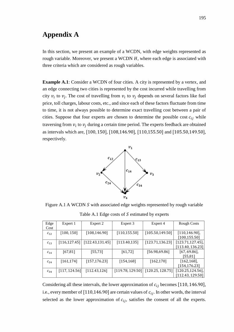
195

Appendix A

In this section, we present an example of a WCDN, with edge weights represented as

rough variable. Moreover, we present a WCDN 𝐻, where each edge is associated with

three criteria which are considered as rough variables.

Example A.1: Consider a WCDN of four cities. A city is represented by a vertex, and

an edge connecting two cities is represented by the cost incurred while travelling from

city 𝑣𝑖 to 𝑣𝑗 . The cost of travelling from 𝑣𝑖 to 𝑣𝑗 depends on several factors like fuel

price, toll charges, labour costs, etc., and since each of these factors fluctuate from time

to time, it is not always possible to determine exact travelling cost between a pair of

cities. Suppose that four experts are chosen to determine the possible cost 𝑐𝑖𝑗 while

traversing from 𝑣𝑖 to 𝑣𝑗 during a certain time period. The experts feedback are obtained

as intervals which are, [100, 150], [108,146.90], [110,155.50] and [105.50,149.50],

respectively.

Figure A.1 A WCDN 𝑆 with associated edge weights represented by rough variable

Table A.1 Edge costs of 𝑆 estimated by experts

Edge

Cost

Expert 1 Expert 2 Expert 3 Expert 4 Rough Costs

𝑐12 [100, 150] [108,146.90] [110,155.50] [105.50,149.50] [110,146.90], [100,155.50]

𝑐13 [116,127.45] [122.43,131.45] [113.40,135] [123.71,136.23] [123.71,127.45], [113.40, 136.23]

𝑐14 [67,81] [55,73] [61,72] [56.98,69.86] [67, 69.86], [55,81]

𝑐24 [161,174] [157,176.23] [154,168] [162,170] [162,168], [154,176.23]

𝑐34 [117, 124.56] [112.43,126] [119.78, 129.50] [120.25, 128.75] [120.25,124.56], [112.43, 129.50]

Considering all these intervals, the lower approximation of 𝑐𝑖𝑗 becomes [110, 146.90],

i.e., every member of [110,146.90] are certain values of 𝑐𝑖𝑗. In other words, the interval

selected as the lower approximation of 𝑐𝑖𝑗, satisfies the consent of all the experts.

User

Text Box

196

Further, the interval, [100,155.50] becomes the upper approximation of 𝑐𝑖𝑗 which

include all the feedback received from the experts such that the elements of

[100,155.50] become the possible values of 𝑐𝑖𝑗. Therefore, 𝑐𝑖𝑗 can be represented by a

rough variable ([110,146.90], [100,155.50]). Fig. A.1 depicts a WCDN 𝑆 for four

cities and the corresponding costs as determined by the experts are shown in Table A.1.

Example A.2: Here, we present a WCDN 𝑅, where each edge is associated with

multiple criteria and are represented by rough variable. Fig. A.2 depicts the WCDN 𝑅

and its corresponding edge weights are reported in Table A.2.

Table A.2 Edge weights of 𝑅: distance, cost and time represented by rough variable

Edges

(𝑒𝑖𝑗)

Distance

(𝑃𝑖𝑗1

= ([𝑃21, 𝑃3

1], [𝑃11, 𝑃4

1]))

Cost

(𝑃𝑖𝑗2

= ([𝑃22, 𝑃3

2], [𝑃12, 𝑃4

2]))

Time

(𝑃𝑖𝑗3

= ([𝑃23, 𝑃3

3], [𝑃13, 𝑃4

3]))

𝑒12 [9,11], [8,15] [21,26], [19,27] [24,27], [23,29] 𝑒13 [17,21], [14,25] [14,15], [12,17] [11,12], [10,14] 𝑒14 [30,36], [27,38] [9,11], [7,12] [30,31], [24,32] 𝑒25 [26,28], [22,33] [14,19], [11,20] [27,28], [26,29] 𝑒37 [8,12], [6,17] [15,18], [14,21] [10,11], [9,15] 𝑒45 [31,35], [29,39] [27,29], [24,30] [26,28], [21,32] 𝑒46 [27,29], [24,36] [12,14], [10,15] [24,26], [20,27] 𝑒58 [36,38], [42,40] [18,19], [17,21] [18,21], [17,29] 𝑒59 [31,33], [29,37] [21,26], [18,27] [21,22], [20,23] 𝑒69 [11,17], [10,21] [18,19], [14,21] [18,19], [17,21] 𝑒710 [30,35], [28,38] [27,29], [24,32] [14,15], [11,17] 𝑒815 [25,28], [24,31] [30,31], [29,34] [21,24], [19,25] 𝑒97 [18,23], [15,27] [8,11], [7,14] [15,17], [14,18] 𝑒98 [27,29], [23,34] [10,15], [9,17] [20,21], [17,22] 𝑒912 [5,8], [4,10] [18,21], [15,23] [31,32], [29,35] 𝑒1013 [11,17], [9,20] [15,18], [12,19] [12,14], [10,17] 𝑒119 [21,26], [18,29] [25,28], [21,30] [28,29], [27,32] 𝑒1112 [28,30], [24,35] [22,24], [20,25] [15,18], [14,17] 𝑒1213 [7,9], [5,11] [12,14], [11,15] [14,17], [12,19] 𝑒1214 [17,18], [15,20] [28,32], [23,34] [11,12], [10,21] 𝑒1311 [28,32], [26,37] [31,34], [29,35] [18,19], [17,21] 𝑒1314 [7,9], [3,14] [27,29], [26,30] [25,28], [24,34] 𝑒1415 [21,27], [22,32] [24,26], [23,28] [18,20], [17,24] 𝑒1416 [35,38], [33,39] [9,11], [8,12] [28,29], [27,30] 𝑒1512 [5,8], [4,11] [28,29], [25,31] [25,26], [24,27] 𝑒1516 [28,29], [24,31] [36,37], [33,39] [21,25], [20,28] 𝑒1517 [41,46], [39,47] [42,45], [41,46] [37,39], [34,46] 𝑒1617 [36,39], [31,42] [39,42], [37,45] [40,42], [39,48]

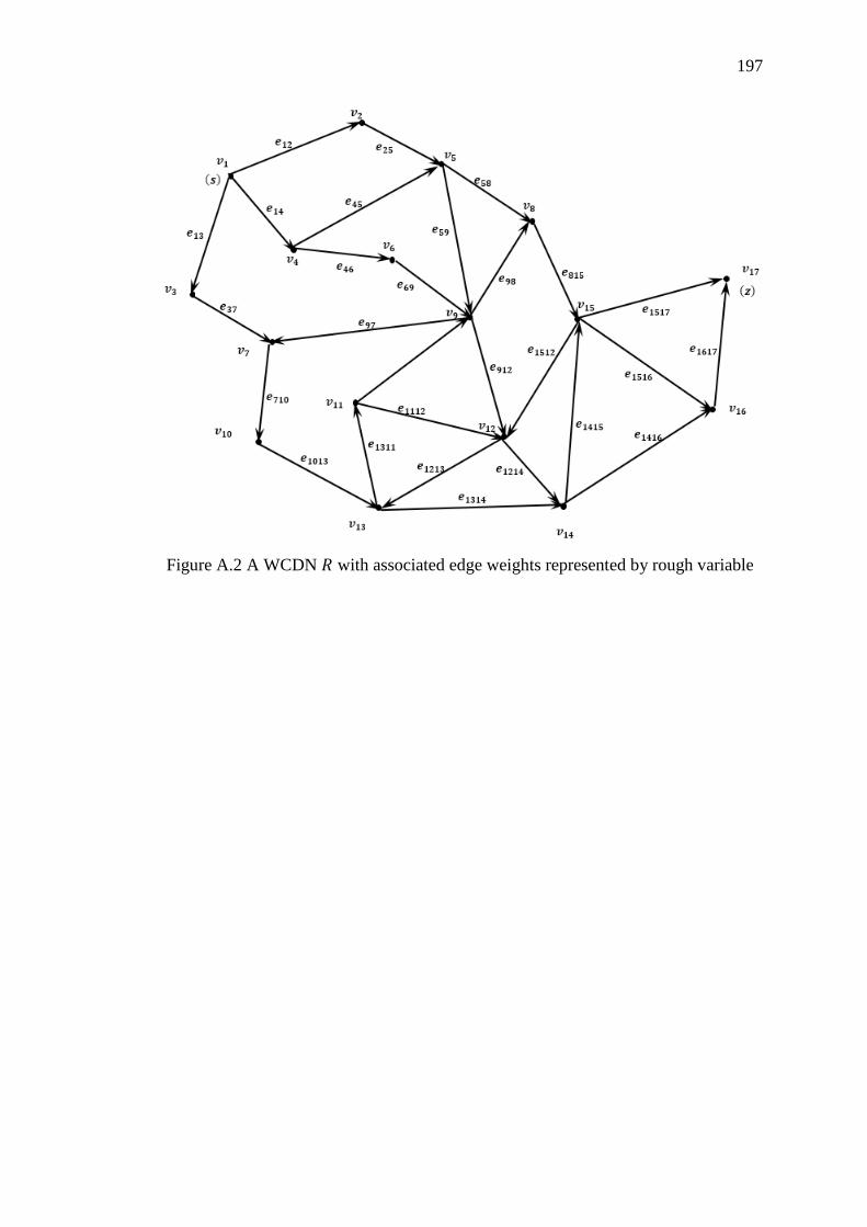
197

Figure A.2 A WCDN 𝑅 with associated edge weights represented by rough variable

198

User

Text Box

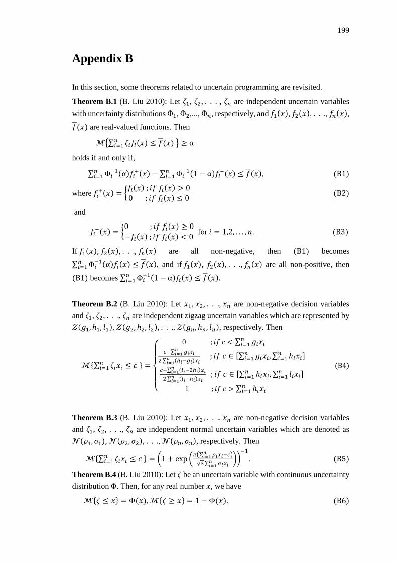
199

Appendix B

In this section, some theorems related to uncertain programming are revisited.

Theorem B.1 (B. Liu 2010): Let 휁1, 휁2, . . . , 휁𝑛 are independent uncertain variables

with uncertainty distributions Φ1, Φ2,..., Φ𝑛, respectively, and 𝑓1(𝑥), 𝑓2(𝑥), . . ., 𝑓𝑛(𝑥),

𝑓(𝑥) are real-valued functions. Then

ℳ{∑ 휁𝑖𝑓𝑖(𝑥)𝑛𝑖=1 ≤ 𝑓(𝑥) } ≥ α

holds if and only if,

∑ Φ𝑖−1(α)𝑓𝑖

+(𝑥)𝑛𝑖=1 − ∑ Φ𝑖

−1(1 − α)𝑓𝑖−(𝑥)𝑛

𝑖=1 ≤ 𝑓(𝑥), (B1)

where 𝑓𝑖+(𝑥) = {

𝑓𝑖(𝑥) ; 𝑖𝑓 𝑓𝑖(𝑥) > 0

0 ; 𝑖𝑓 𝑓𝑖(𝑥) ≤ 0 (B2)

and

𝑓𝑖−(𝑥) = {

0 ; 𝑖𝑓 𝑓𝑖(𝑥) ≥ 0

−𝑓𝑖(𝑥) ; 𝑖𝑓 𝑓𝑖(𝑥) < 0 for 𝑖 = 1,2, . . . , 𝑛. (B3)

If 𝑓1(𝑥), 𝑓2(𝑥), . . ., 𝑓𝑛(𝑥) are all non-negative, then (B1) becomes

∑ Φ𝑖−1(α)𝑓𝑖(𝑥)

𝑛𝑖=1 ≤ 𝑓(𝑥), and if 𝑓1(𝑥), 𝑓2(𝑥), . . ., 𝑓𝑛(𝑥) are all non-positive, then

(B1) becomes ∑ Φ𝑖−1(1 − α)𝑓𝑖(𝑥)

𝑛𝑖=1 ≤ 𝑓(𝑥).

Theorem B.2 (B. Liu 2010): Let 𝑥1, 𝑥2, . . ., 𝑥𝑛 are non-negative decision variables

and 휁1, 휁2, . . ., 휁𝑛 are independent zigzag uncertain variables which are represented by

𝒵(𝑔1, ℎ1, 𝑙1), 𝒵(𝑔2, ℎ2, 𝑙2), . . ., 𝒵(𝑔𝑛, ℎ𝑛, 𝑙𝑛), respectively. Then

ℳ{∑ 휁𝑖𝑥𝑖𝑛𝑖=1 ≤ 𝑐 } =

{

0 ; 𝑖𝑓 𝑐 < ∑ 𝑔𝑖𝑥𝑖𝑛𝑖=1

𝑐−∑ 𝑔𝑖𝑥𝑖𝑛𝑖=1

2∑ (ℎ𝑖−𝑔𝑖)𝑥𝑖𝑛𝑖=1

; 𝑖𝑓 𝑐 ∈ [∑ 𝑔𝑖𝑥𝑖 , ∑ ℎ𝑖𝑥𝑖𝑛𝑖=1

𝑛𝑖=1 ]

𝑐+∑ (𝑙𝑖−2ℎ𝑖)𝑥𝑖𝑛𝑖=1

2∑ (𝑙𝑖−ℎ𝑖)𝑥𝑖𝑛𝑖=1

; 𝑖𝑓 𝑐 ∈ [∑ ℎ𝑖𝑥𝑖 , ∑ 𝑙𝑖𝑥𝑖𝑛𝑖=1

𝑛𝑖=1 ]

1 ; 𝑖𝑓 𝑐 > ∑ ℎ𝑖𝑥𝑖𝑛𝑖=1

(B4)

Theorem B.3 (B. Liu 2010): Let 𝑥1, 𝑥2, . . ., 𝑥𝑛 are non-negative decision variables

and 휁1, 휁2, . . ., 휁𝑛 are independent normal uncertain variables which are denoted as

𝒩(𝜌1, 𝜎1), 𝒩(𝜌2, 𝜎2), . . ., 𝒩(𝜌𝑛, 𝜎𝑛), respectively. Then

ℳ{∑ 휁𝑖𝑥𝑖𝑛𝑖=1 ≤ 𝑐 } = (1 + exp (

𝜋(∑ 𝜌𝑖𝑥𝑖−𝑐𝑛𝑖=1 )

√3∑ 𝜎𝑖𝑥𝑖𝑛𝑖=1

))−1

. (B5)

Theorem B.4 (B. Liu 2010): Let 휁 be an uncertain variable with continuous uncertainty

distribution Φ. Then, for any real number 𝑥, we have

ℳ{휁 ≤ 𝑥} = Φ(𝑥), ℳ{휁 ≥ 𝑥} = 1 − Φ(𝑥). (B6)

User

Text Box

200

User

Text Box

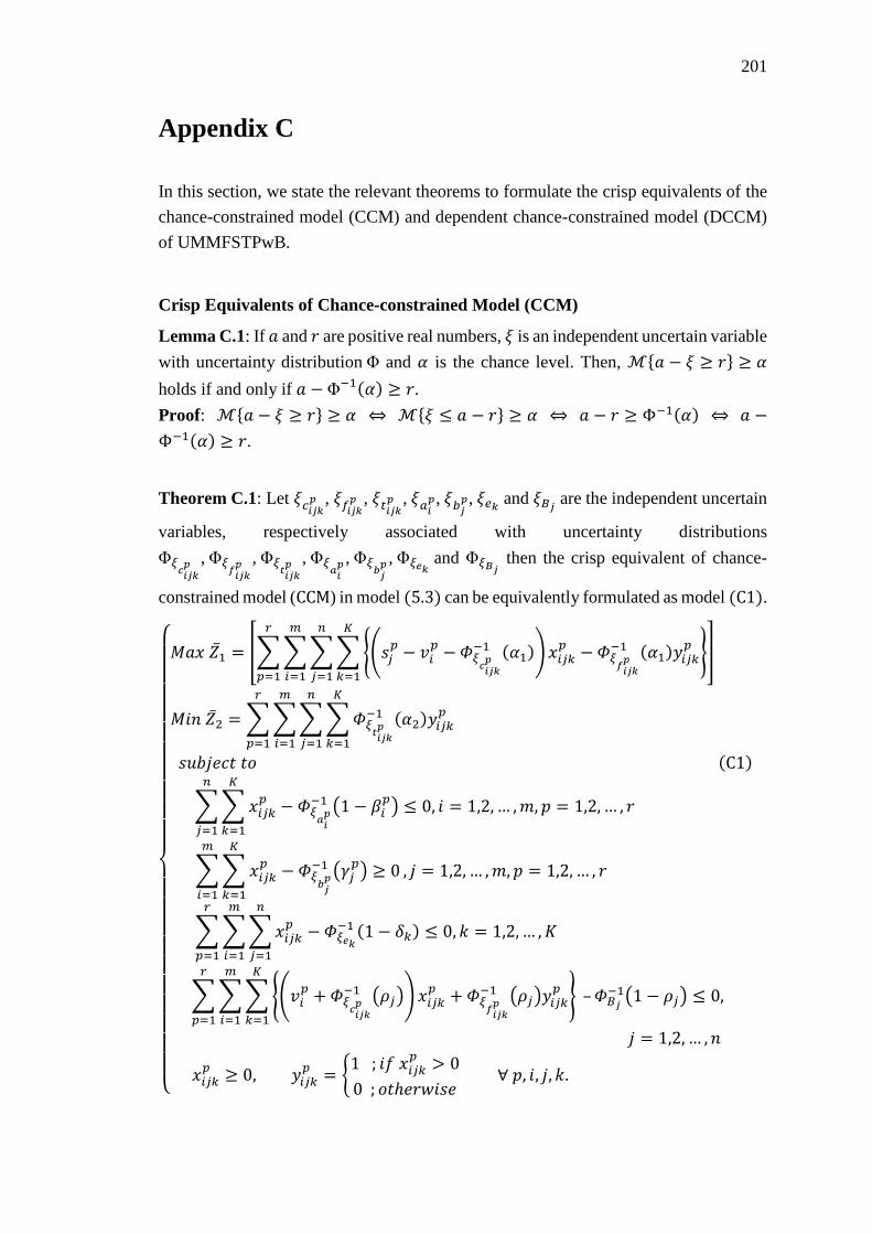
201

Appendix C

In this section, we state the relevant theorems to formulate the crisp equivalents of the

chance-constrained model (CCM) and dependent chance-constrained model (DCCM)

of UMMFSTPwB.

Crisp Equivalents of Chance-constrained Model (CCM)

Lemma C.1: If 𝑎 and 𝑟 are positive real numbers, 𝜉 is an independent uncertain variable

with uncertainty distribution Φ and 𝛼 is the chance level. Then, ℳ{𝑎 − 𝜉 ≥ 𝑟} ≥ 𝛼

holds if and only if 𝑎 − Φ−1(𝛼) ≥ 𝑟.

Proof: ℳ{𝑎 − 𝜉 ≥ 𝑟} ≥ 𝛼 ⇔ ℳ{𝜉 ≤ 𝑎 − 𝑟} ≥ 𝛼 ⇔ 𝑎 − 𝑟 ≥ Φ−1(𝛼) ⇔ 𝑎 −

Φ−1(𝛼) ≥ 𝑟.

Theorem C.1: Let 𝜉𝑐𝑖𝑗𝑘𝑝 , 𝜉𝑓𝑖𝑗𝑘


𝑝, 𝜉𝑏𝑗𝑝, 𝜉𝑒𝑘 and 𝜉𝐵𝑗 are the independent uncertain

variables, respectively associated with uncertainty distributions

Φ𝜉𝑐𝑖𝑗𝑘𝑝 , Φ𝜉

𝑓𝑖𝑗𝑘𝑝 , Φ𝜉

𝑡𝑖𝑗𝑘𝑝 , Φ𝜉

𝑎𝑖𝑝 , Φ𝜉

𝑏𝑗𝑝 , Φ𝜉𝑒𝑘

and Φ𝜉𝐵𝑗 then the crisp equivalent of chance-

constrained model (CCM) in model (5.3) can be equivalently formulated as model (C1).

{

𝑀𝑎𝑥 ��1 = [∑∑∑∑{(𝑠𝑗

𝑝 − 𝑣𝑖𝑝 − 𝛷𝜉


−1 (𝛼1))𝑥𝑖𝑗𝑘𝑝 − 𝛷𝜉


−1 (𝛼1)𝑦𝑖𝑗𝑘𝑝 }

𝐾

𝑘=1

𝑛

𝑗=1

𝑚

𝑖=1

𝑟

𝑝=1

]

𝑀𝑖𝑛 ��2 =∑∑∑∑𝛷𝜉𝑡𝑖𝑗𝑘𝑝

−1 (𝛼2)𝑦𝑖𝑗𝑘𝑝

𝐾

𝑘=1

𝑛

𝑗=1

𝑚

𝑖=1

𝑟

𝑝=1

𝑠𝑢𝑏𝑗𝑒𝑐𝑡 𝑡𝑜 (C1)

∑∑𝑥𝑖𝑗𝑘𝑝 − 𝛷𝜉

𝑎𝑖𝑝

−1 (1 − 𝛽𝑖𝑝)

𝐾

𝑘=1

𝑛

𝑗=1

≤ 0, 𝑖 = 1,2, … ,𝑚, 𝑝 = 1,2, … , 𝑟

∑∑𝑥𝑖𝑗𝑘𝑝 − 𝛷𝜉

𝑏𝑗𝑝

−1 (𝛾𝑗𝑝) ≥ 0

𝐾

𝑘=1

𝑚

𝑖=1

, 𝑗 = 1,2, … ,𝑚, 𝑝 = 1,2, … , 𝑟


𝑛

𝑗=1

− 𝛷𝜉𝑒𝑘−1 (1 − 𝛿𝑘)

𝑚

𝑖=1

𝑟

𝑝=1

≤ 0, 𝑘 = 1,2, … , 𝐾

∑∑∑{(𝑣𝑖𝑝 + 𝛷𝜉


−1 (𝜌𝑗)) 𝑥𝑖𝑗𝑘𝑝 + 𝛷𝜉


−1 (𝜌𝑗)𝑦𝑖𝑗𝑘𝑝 }

𝐾

𝑘=1

𝑚

𝑖=1

𝑟

𝑝=1

– 𝛷𝐵𝑗−1(1 − 𝜌𝑗) ≤ 0,

𝑗 = 1,2, … , 𝑛



𝑝 > 0


User

Text Box

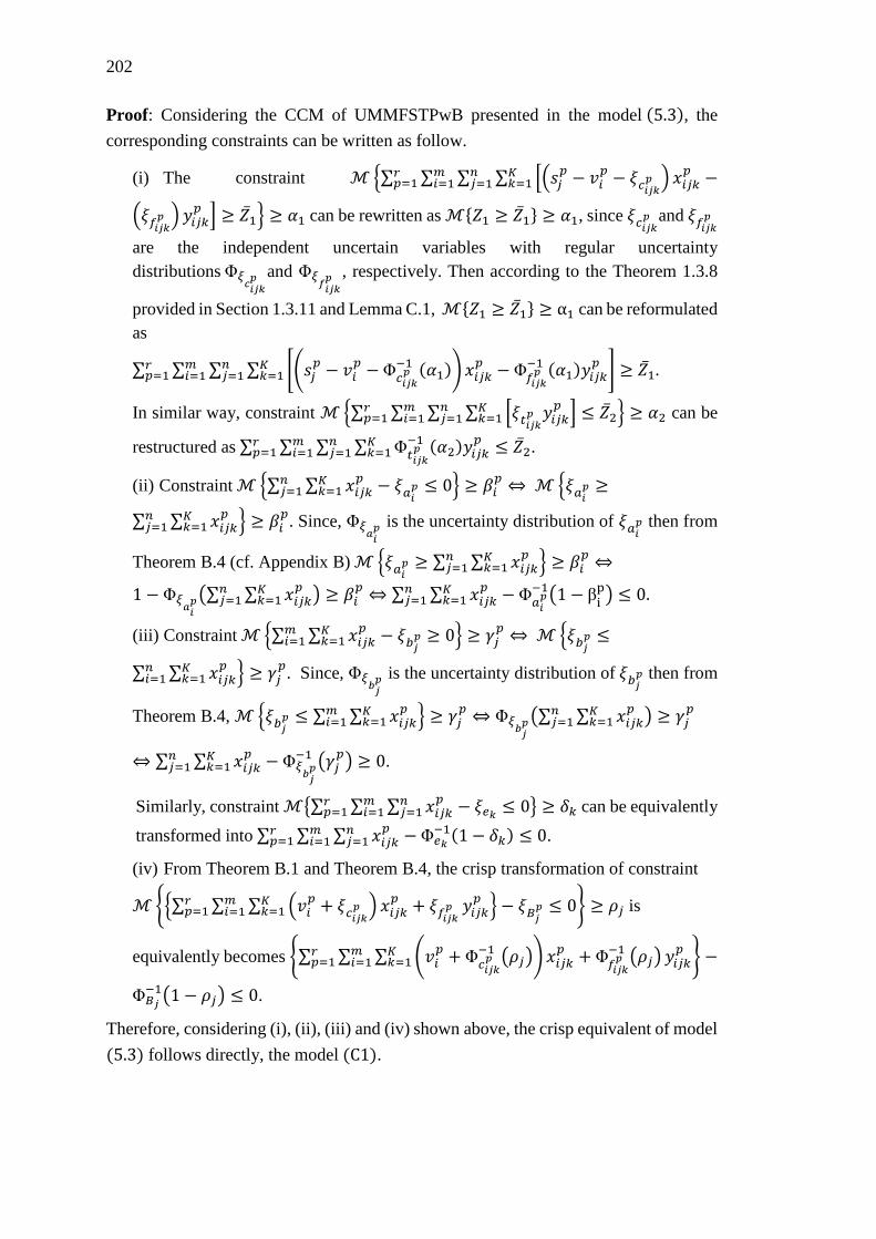
202

Proof: Considering the CCM of UMMFSTPwB presented in the model (5.3), the

corresponding constraints can be written as follow.

(i) The constraint ℳ{∑ ∑ ∑ ∑ [(𝑠𝑗𝑝 − 𝑣𝑖


𝑝 −𝐾𝑘=1

𝑛𝑗=1

𝑚𝑖=1

𝑟𝑝=1

(𝜉𝑓𝑖𝑗𝑘𝑝 ) 𝑦𝑖𝑗𝑘

𝑝 ] ≥ ��1} ≥ 𝛼1 can be rewritten as ℳ{𝑍1 ≥ ��1} ≥ 𝛼1, since 𝜉𝑐𝑖𝑗𝑘𝑝 and 𝜉𝑓𝑖𝑗𝑘

𝑝

are the independent uncertain variables with regular uncertainty

distributions Φ𝜉𝑐𝑖𝑗𝑘𝑝 and Φ𝜉

𝑓𝑖𝑗𝑘𝑝 , respectively. Then according to the Theorem 1.3.8

provided in Section 1.3.11 and Lemma C.1, ℳ{𝑍1 ≥ ��1} ≥ α1 can be reformulated

as

∑ ∑ ∑ ∑ [(𝑠𝑗𝑝 − 𝑣𝑖

𝑝 − Φ𝑐𝑖𝑗𝑘𝑝−1 (𝛼1)) 𝑥𝑖𝑗𝑘

𝑝 − Φ𝑓𝑖𝑗𝑘𝑝−1 (𝛼1)𝑦𝑖𝑗𝑘

𝑝 ]𝐾𝑘=1

𝑛𝑗=1

𝑚𝑖=1

𝑟𝑝=1 ≥ ��1.

In similar way, constraint ℳ{∑ ∑ ∑ ∑ [𝜉𝑡𝑖𝑗𝑘𝑝 𝑦𝑖𝑗𝑘

𝑝 ]𝐾𝑘=1

𝑛𝑗=1

𝑚𝑖=1

𝑟𝑝=1 ≤ ��2} ≥ 𝛼2 can be

restructured as ∑ ∑ ∑ ∑ Φ𝑡𝑖𝑗𝑘𝑝−1 (𝛼2)𝑦𝑖𝑗𝑘

𝑝𝐾𝑘=1

𝑛𝑗=1

𝑚𝑖=1

𝑟𝑝=1 ≤ ��2.

(ii) Constraint ℳ {∑ ∑ 𝑥𝑖𝑗𝑘𝑝 − 𝜉𝑎𝑖

𝑝𝐾𝑘=1

𝑛𝑗=1 ≤ 0} ≥ 𝛽𝑖

𝑝 ⇔ ℳ {𝜉𝑎𝑖𝑝 ≥

∑ ∑ 𝑥𝑖𝑗𝑘𝑝𝐾

𝑘=1𝑛𝑗=1 } ≥ 𝛽𝑖

𝑝. Since, Φ𝜉

𝑎𝑖𝑝 is the uncertainty distribution of 𝜉𝑎𝑖

𝑝 then from

Theorem B.4 (cf. Appendix B) ℳ {𝜉𝑎𝑖𝑝 ≥ ∑ ∑ 𝑥𝑖𝑗𝑘

𝑝𝐾𝑘=1

𝑛𝑗=1 } ≥ 𝛽𝑖

𝑝 ⇔

1 − Φ𝜉𝑎𝑖𝑝(∑ ∑ 𝑥𝑖𝑗𝑘

𝑝𝐾𝑘=1

𝑛𝑗=1 ) ≥ 𝛽𝑖

𝑝 ⇔ ∑ ∑ 𝑥𝑖𝑗𝑘𝑝𝐾

𝑘=1𝑛𝑗=1 − Φ

𝑎𝑖𝑝−1(1 − β

ip) ≤ 0.

(iii) Constraint ℳ {∑ ∑ 𝑥𝑖𝑗𝑘𝑝 − 𝜉𝑏𝑗

𝑝𝐾𝑘=1

𝑚𝑖=1 ≥ 0} ≥ 𝛾𝑗

𝑝 ⇔ ℳ {𝜉𝑏𝑗𝑝 ≤

∑ ∑ 𝑥𝑖𝑗𝑘𝑝𝐾

𝑘=1𝑛𝑖=1 } ≥ 𝛾𝑗

𝑝. Since, Φ𝜉

𝑏𝑗𝑝 is the uncertainty distribution of 𝜉𝑏𝑗

𝑝 then from

Theorem B.4, ℳ{𝜉𝑏𝑗𝑝 ≤ ∑ ∑ 𝑥𝑖𝑗𝑘

𝑝𝐾𝑘=1

𝑚𝑖=1 } ≥ 𝛾𝑗

𝑝 ⇔ Φ𝜉𝑏𝑗𝑝(∑ ∑ 𝑥𝑖𝑗𝑘

𝑝𝐾𝑘=1

𝑛𝑗=1 ) ≥ 𝛾𝑗

𝑝

⇔ ∑ ∑ 𝑥𝑖𝑗𝑘𝑝𝐾

𝑘=1𝑛𝑗=1 − Φ𝜉

𝑏𝑗𝑝

−1 (𝛾𝑗𝑝) ≥ 0.

Similarly, constraint ℳ{∑ ∑ ∑ 𝑥𝑖𝑗𝑘𝑝𝑛


𝑟𝑝=1 ≤ 0} ≥ 𝛿𝑘 can be equivalently

transformed into ∑ ∑ ∑ 𝑥𝑖𝑗𝑘𝑝𝑛

𝑗=1 − Φ𝑒𝑘−1(1 − 𝛿𝑘)

𝑚𝑖=1

𝑟𝑝=1 ≤ 0.

(iv) From Theorem B.1 and Theorem B.4, the crisp transformation of constraint

ℳ{{∑ ∑ ∑ (𝑣𝑖𝑝 + 𝜉𝑐𝑖𝑗𝑘

𝑝 ) 𝑥𝑖𝑗𝑘𝑝𝐾

𝑘=1 + 𝜉𝑓𝑖𝑗𝑘𝑝

𝑚𝑖=1 𝑦𝑖𝑗𝑘

𝑝𝑟𝑝=1 } − 𝜉𝐵𝑗

𝑝 ≤ 0} ≥ 𝜌𝑗 is

equivalently becomes {∑ ∑ ∑ (𝑣𝑖𝑝+ Φ

𝑐𝑖𝑗𝑘𝑝−1 (𝜌𝑗)) 𝑥𝑖𝑗𝑘

𝑝𝐾𝑘=1 + Φ

𝑓𝑖𝑗𝑘𝑝−1 (𝜌𝑗)

𝑚𝑖=1 𝑦𝑖𝑗𝑘

𝑝𝑟𝑝=1 } −

Φ𝐵𝑗−1(1 − 𝜌𝑗) ≤ 0.

Therefore, considering (i), (ii), (iii) and (iv) shown above, the crisp equivalent of model

(5.3) follows directly, the model (C1).

203

Corollary C.1: If 𝜉𝑐𝑖𝑗𝑘𝑝 , 𝜉𝑓𝑖𝑗𝑘


𝑝, 𝜉𝑏𝑗𝑝, 𝜉𝑒𝑘

𝑝 and 𝜉𝐵𝑗𝑝 are the independent zigzag

uncertain variables of the form 𝒵(𝑔, ℎ, 𝑙) with 𝑔 < ℎ < 𝑙. Then, according to Theorem

C.1 and the inverse uncertainty distribution of zigzag uncertain variables, we can

conclude the following.

(i) For all chance levels <0.5, model (C1) becomes

{

𝑀𝑎𝑥 ��1 = ∑∑∑∑[(𝑠𝑗

𝑝− 𝑣𝑖

𝑝− ((1 − 2𝛼1)𝑔𝑐𝑖𝑗𝑘

𝑝 + 2𝛼1ℎ𝑐𝑖𝑗𝑘𝑝 )) 𝑥𝑖𝑗𝑘

𝑝− ((1 − 2𝛼1)𝑔𝑓𝑖𝑗𝑘

𝑝 + 2𝛼1ℎ𝑓𝑖𝑗𝑘𝑝 ) 𝑦𝑖𝑗𝑘

𝑝]

𝐾

𝑘=1

𝑛

𝑗=1

𝑚

𝑖=1

𝑟

𝑝=1

𝑀𝑖𝑛 ��2 =∑∑∑∑[((1 − 2𝛼2)𝑔𝑡𝑖𝑗𝑘𝑝 + 2𝛼2ℎ𝑡𝑖𝑗𝑘

𝑝 )𝑦𝑖𝑗𝑘𝑝]

𝐾

𝑘=1

𝑛

𝑗=1

𝑚

𝑖=1

𝑟

𝑝=1


∑∑𝑥𝑖𝑗𝑘𝑝− (2𝛽𝑖

𝑝ℎ𝑎𝑖

𝑝 + (1 − 2𝛽𝑖𝑝)𝑙𝑎𝑖

𝑝)

𝐾

𝑘=1

𝑛

𝑗=1

≤ 0, 𝑖 = 1,2, … ,𝑚, 𝑝 = 1,2,… , 𝑟

∑∑𝑥𝑖𝑗𝑘𝑝− ((1 − 2𝛾𝑗

𝑝)𝑔𝑏𝑗

𝑝 + 2𝛾𝑗𝑝ℎ𝑏𝑗

𝑝) ≥ 0

𝐾

𝑘=1

𝑚

𝑖=1

, 𝑗 = 1,2,… , 𝑛, 𝑝 = 1,2,… , 𝑟


𝑛

𝑗=1

− (2𝛿𝑘ℎ𝑒𝑘 + (1 − 2𝛿𝑘)𝑙𝑒𝑘)

𝑚

𝑖=1

𝑟

𝑝=1

≤ 0, 𝑘 = 1,2,… , 𝐾

∑∑∑[𝑣𝑖𝑝+ ((1 − 2𝜌𝑗)𝑔𝑐𝑖𝑗𝑘

𝑝 + 2𝜌𝑗𝑝ℎ𝑐𝑖𝑗𝑘

𝑝 )] 𝑥𝑖𝑗𝑘𝑝

𝐾

𝑘=1

+ [((1 − 2𝜌𝑗)𝑔𝑓𝑖𝑗𝑘𝑝 + 2𝜌𝑗ℎ𝑓𝑖𝑗𝑘

𝑝 )]

𝑚

𝑖=1

𝑦𝑖𝑗𝑘𝑝

𝑟

𝑝=1

− (2𝜌𝑗ℎ𝐵𝑗 + (1 − 2𝜌𝑗)𝑙𝐵𝑗) ≤ 0, 𝑗 = 1,2,… , 𝑛


𝑝= {



(ii) For all chance levels ≥ 0.5, model (C1) can be described as given in (C3).

{

𝑀𝑎𝑥 ��1 = ∑∑∑∑[(𝑠𝑗

𝑝− 𝑣𝑖

𝑝− ((2 − 2α1)ℎ𝑐𝑖𝑗𝑘

𝑝 + (2𝛼1 − 1)𝑙𝑐𝑖𝑗𝑘𝑝 ))𝑥𝑖𝑗𝑘

𝑝− ((2 − 2𝛼1)ℎ𝑓𝑖𝑗𝑘

𝑝 + (2𝛼1 − 1)𝑙𝑓𝑖𝑗𝑘𝑝 )𝑦𝑖𝑗𝑘

𝑝]

𝐾

𝑘=1

𝑛

𝑗=1

𝑚

𝑖=1

𝑟

𝑝=1

𝑀𝑖𝑛 ��2 = ∑∑∑∑[((2 − 2𝛼2)ℎ𝑡𝑖𝑗𝑘𝑝 + (2𝛼2 − 1)𝑙𝑡𝑖𝑗𝑘

𝑝 )𝑦𝑖𝑗𝑘𝑝]

𝐾

𝑘=1

𝑛

𝑗=1

𝑚

𝑖=1

𝑟

𝑝=1


∑∑𝑥𝑖𝑗𝑘𝑝− ((2𝛽𝑖

𝑝− 1)𝑔𝑎𝑖

𝑝 + (2 − 2𝛽𝑖𝑝)ℎ𝑎𝑖

𝑝)

𝐾

𝑘=1

𝑛

𝑗=1

≤ 0, 𝑖 = 1,2, … ,𝑚, 𝑝 = 1,2,… , 𝑟

∑∑𝑥𝑖𝑗𝑘𝑝− ((2 − 2𝛾𝑗

𝑝)ℎ𝑏𝑗

𝑝 + (2𝛾𝑗𝑝− 1)𝑙𝑏𝑗

𝑝) ≥ 0

𝐾

𝑘=1

𝑚

𝑖=1

, 𝑗 = 1,2,… , 𝑛, 𝑝 = 1,2,… , 𝑟


𝑛

𝑗=1

− ((2𝛿𝑘 − 1)𝑔𝑒𝑘 + (2 − 2𝛿𝑘)ℎ𝑒𝑘)

𝑚

𝑖=1

𝑟

𝑝=1

≤ 0, 𝑘 = 1,2,… , 𝐾

∑∑∑[𝑣𝑖𝑝+ ((2 − 2𝜌𝑗)ℎ𝑐𝑖𝑗𝑘

𝑝 + (2𝜌𝑗 − 1)𝑙𝑐𝑖𝑗𝑘𝑝 )] 𝑥𝑖𝑗𝑘

𝑝

𝐾

𝑘=1

+ [(2 − 2𝜌𝑗)ℎ𝑓𝑖𝑗𝑘𝑝 + (2𝜌𝑗 − 1)𝑙𝑓𝑖𝑗𝑘

𝑝 ]

𝑚

𝑖=1

𝑦𝑖𝑗𝑘𝑝

𝑟

𝑝=1

−((2𝜌𝑗 − 1)𝑔𝐵𝑗 + (2 − 2𝜌𝑗)ℎ𝐵𝑗) ≤ 0, 𝑗 = 1,2,… , 𝑛


𝑝= {



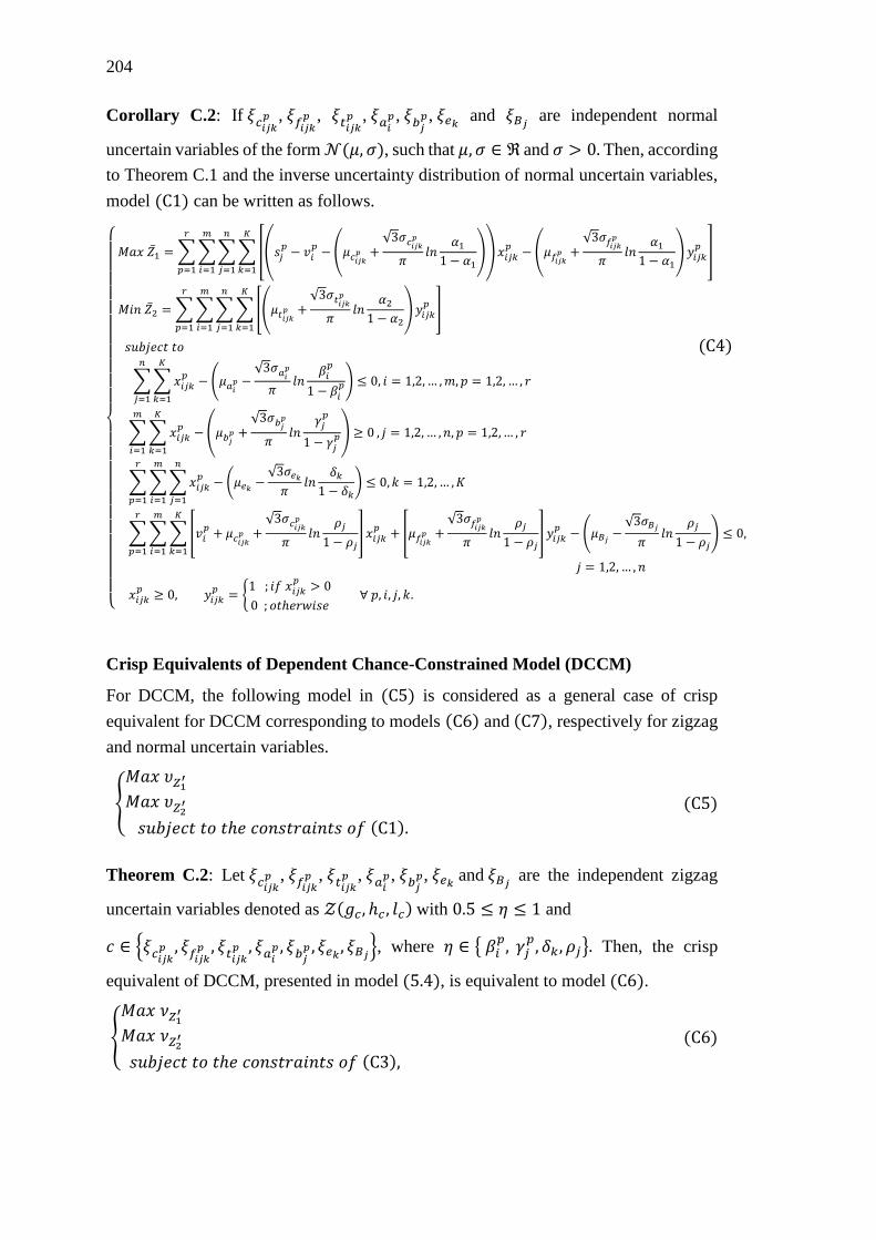
204

Corollary C.2: If 𝜉𝑐𝑖𝑗𝑘𝑝 , 𝜉𝑓𝑖𝑗𝑘


𝑝, 𝜉𝑏𝑗𝑝, 𝜉𝑒𝑘 and 𝜉𝐵𝑗 are independent normal

uncertain variables of the form 𝒩(𝜇, 𝜎), such that 𝜇, 𝜎 ∈ ℜ and 𝜎 > 0. Then, according

to Theorem C.1 and the inverse uncertainty distribution of normal uncertain variables,

model (C1) can be written as follows.

{

𝑀𝑎𝑥 ��1 = ∑∑∑∑[(𝑠𝑗

𝑝− 𝑣𝑖

𝑝−(𝜇𝑐𝑖𝑗𝑘

𝑝 +√3𝜎𝑐𝑖𝑗𝑘

𝑝

𝜋𝑙𝑛

𝛼11 − 𝛼1

))𝑥𝑖𝑗𝑘𝑝− (𝜇𝑓𝑖𝑗𝑘

𝑝 +√3𝜎𝑓𝑖𝑗𝑘

𝑝

𝜋𝑙𝑛

𝛼11 − 𝛼1

)𝑦𝑖𝑗𝑘𝑝]

𝐾

𝑘=1

𝑛

𝑗=1

𝑚

𝑖=1

𝑟

𝑝=1

𝑀𝑖𝑛 ��2 = ∑∑∑∑[(𝜇𝑡𝑖𝑗𝑘𝑝 +

√3𝜎𝑡𝑖𝑗𝑘𝑝

𝜋𝑙𝑛

𝛼21 − 𝛼2

)𝑦𝑖𝑗𝑘𝑝]

𝐾

𝑘=1

𝑛

𝑗=1

𝑚

𝑖=1

𝑟

𝑝=1


∑∑𝑥𝑖𝑗𝑘𝑝− (𝜇𝑎𝑖

𝑝 −√3𝜎𝑎𝑖

𝑝

𝜋𝑙𝑛

𝛽𝑖𝑝

1 − 𝛽𝑖𝑝)

𝐾

𝑘=1

𝑛

𝑗=1

≤ 0, 𝑖 = 1,2,… ,𝑚, 𝑝 = 1,2, … , 𝑟

∑∑𝑥𝑖𝑗𝑘𝑝−(𝜇𝑏𝑗

𝑝 +√3𝜎𝑏𝑗

𝑝

𝜋𝑙𝑛

𝛾𝑗𝑝

1 − 𝛾𝑗𝑝) ≥ 0

𝐾

𝑘=1

𝑚

𝑖=1

, 𝑗 = 1,2, … , 𝑛, 𝑝 = 1,2,… , 𝑟


𝑛

𝑗=1

− (𝜇𝑒𝑘 −√3𝜎𝑒𝑘𝜋

𝑙𝑛𝛿𝑘

1 − 𝛿𝑘)

𝑚

𝑖=1

𝑟

𝑝=1

≤ 0, 𝑘 = 1,2, … ,𝐾

∑∑∑[𝑣𝑖𝑝+ 𝜇𝑐𝑖𝑗𝑘

𝑝 +√3𝜎𝑐𝑖𝑗𝑘

𝑝

𝜋𝑙𝑛

𝜌𝑗

1 − 𝜌𝑗] 𝑥𝑖𝑗𝑘

𝑝

𝐾

𝑘=1

+ [𝜇𝑓𝑖𝑗𝑘𝑝 +

√3𝜎𝑓𝑖𝑗𝑘𝑝

𝜋𝑙𝑛

𝜌𝑗

1 − 𝜌𝑗]

𝑚

𝑖=1

𝑦𝑖𝑗𝑘𝑝− (𝜇𝐵𝑗 −

√3𝜎𝐵𝑗𝜋

𝑙𝑛𝜌𝑗

1 − 𝜌𝑗) ≤ 0,

𝑟

𝑝=1

𝑗 = 1,2, … , 𝑛


𝑝= {



Crisp Equivalents of Dependent Chance-Constrained Model (DCCM)

For DCCM, the following model in (C5) is considered as a general case of crisp

equivalent for DCCM corresponding to models (C6) and (C7), respectively for zigzag

and normal uncertain variables.

{

𝑀𝑎𝑥 𝜐𝑍1′

𝑀𝑎𝑥 𝜐𝑍2′

𝑠𝑢𝑏𝑗𝑒𝑐𝑡 𝑡𝑜 𝑡ℎ𝑒 𝑐𝑜𝑛𝑠𝑡𝑟𝑎𝑖𝑛𝑡𝑠 𝑜𝑓 (C1).

(C5)



𝑝, 𝜉𝑏𝑗𝑝, 𝜉𝑒𝑘 and 𝜉𝐵𝑗 are the independent zigzag

uncertain variables denoted as 𝒵(𝑔𝑐, ℎ𝑐 , 𝑙𝑐) with 0.5 ≤ 휂 ≤ 1 and

𝑐 ∈ {𝜉𝑐𝑖𝑗𝑘𝑝 , 𝜉𝑓𝑖𝑗𝑘


𝑝 , 𝜉𝑏𝑗𝑝 , 𝜉𝑒𝑘 , 𝜉𝐵𝑗}, where 휂 ∈ { 𝛽𝑖

𝑝, 𝛾𝑗𝑝, 𝛿𝑘, 𝜌𝑗}. Then, the crisp

equivalent of DCCM, presented in model (5.4), is equivalent to model (C6).

{

𝑀𝑎𝑥 𝜈𝑍1′

𝑀𝑎𝑥 𝜈𝑍2′

𝑠𝑢𝑏𝑗𝑒𝑐𝑡 𝑡𝑜 𝑡ℎ𝑒 𝑐𝑜𝑛𝑠𝑡𝑟𝑎𝑖𝑛𝑡𝑠 𝑜𝑓 (C3),

(C6)

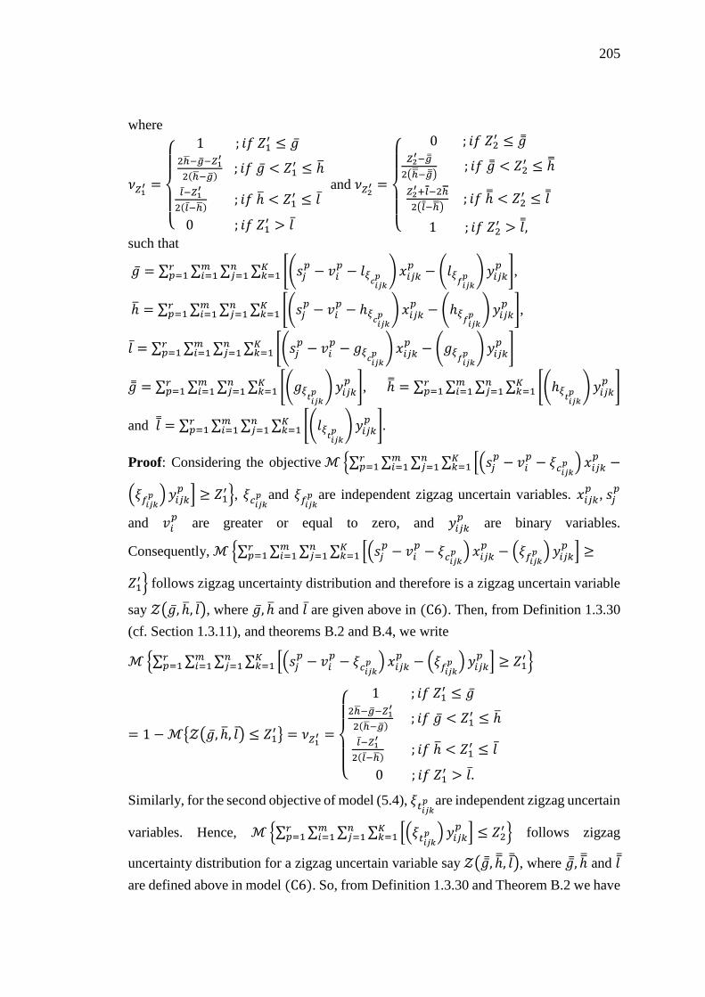
205

where

𝜈𝑍1′ =

{

1 ; 𝑖𝑓 𝑍1′ ≤ ��

2ℎ−��−𝑍1′

2(ℎ−��) ; 𝑖𝑓 �� < 𝑍1

′ ≤ ℎ

𝑙−𝑍1′

2(𝑙−ℎ) ; 𝑖𝑓 ℎ < 𝑍1

′ ≤ 𝑙

0 ; 𝑖𝑓 𝑍1′ > 𝑙

and 𝜈𝑍2′ =

{

0 ; 𝑖𝑓 𝑍2′ ≤ ��

𝑍2′−��

2(ℎ−��) ; 𝑖𝑓 �� < 𝑍2

′ ≤ ℎ

𝑍2′+𝑙−2ℎ

2(𝑙−ℎ) ; 𝑖𝑓 ℎ < 𝑍2

′ ≤ 𝑙

1 ; 𝑖𝑓 𝑍2′ > 𝑙,

such that

�� = ∑ ∑ ∑ ∑ [(𝑠𝑗𝑝 − 𝑣𝑖

𝑝 − 𝑙𝜉𝑐𝑖𝑗𝑘𝑝 ) 𝑥𝑖𝑗𝑘

𝑝 − (𝑙𝜉𝑓𝑖𝑗𝑘𝑝 )𝑦𝑖𝑗𝑘

𝑝 ]𝐾𝑘=1

𝑛𝑗=1

𝑚𝑖=1

𝑟𝑝=1 ,

ℎ = ∑ ∑ ∑ ∑ [(𝑠𝑗𝑝 − 𝑣𝑖

𝑝 − ℎ𝜉𝑐𝑖𝑗𝑘𝑝 ) 𝑥𝑖𝑗𝑘

𝑝 − (ℎ𝜉𝑓𝑖𝑗𝑘𝑝 )𝑦𝑖𝑗𝑘

𝑝 ]𝐾𝑘=1

𝑛𝑗=1

𝑚𝑖=1

𝑟𝑝=1 ,

𝑙 = ∑ ∑ ∑ ∑ [(𝑠𝑗𝑝 − 𝑣𝑖

𝑝 − 𝑔𝜉𝑐𝑖𝑗𝑘𝑝 ) 𝑥𝑖𝑗𝑘

𝑝 − (𝑔𝜉𝑓𝑖𝑗𝑘𝑝 )𝑦𝑖𝑗𝑘

𝑝 ]𝐾𝑘=1

𝑛𝑗=1

𝑚𝑖=1

𝑟𝑝=1

�� = ∑ ∑ ∑ ∑ [(𝑔𝜉𝑡𝑖𝑗𝑘𝑝 )𝑦𝑖𝑗𝑘

𝑝 ]𝐾𝑘=1

𝑛𝑗=1

𝑚𝑖=1

𝑟𝑝=1 , ℎ = ∑ ∑ ∑ ∑ [(ℎ𝜉

𝑡𝑖𝑗𝑘𝑝 )𝑦𝑖𝑗𝑘

𝑝 ]𝐾𝑘=1

𝑛𝑗=1

𝑚𝑖=1

𝑟𝑝=1

and 𝑙 = ∑ ∑ ∑ ∑ [(𝑙𝜉𝑡𝑖𝑗𝑘𝑝 )𝑦𝑖𝑗𝑘

𝑝 ]𝐾𝑘=1

𝑛𝑗=1

𝑚𝑖=1

𝑟𝑝=1 .

Proof: Considering the objective ℳ {∑ ∑ ∑ ∑ [(𝑠𝑗𝑝 − 𝑣𝑖


𝑝 −𝐾𝑘=1

𝑛𝑗=1

𝑚𝑖=1

𝑟𝑝=1

(𝜉𝑓𝑖𝑗𝑘𝑝 ) 𝑦𝑖𝑗𝑘

𝑝 ] ≥ 𝑍1′}, 𝜉𝑐𝑖𝑗𝑘

𝑝 and 𝜉𝑓𝑖𝑗𝑘𝑝 are independent zigzag uncertain variables. 𝑥𝑖𝑗𝑘

𝑝, 𝑠𝑗

𝑝

and 𝑣𝑖𝑝 are greater or equal to zero, and 𝑦𝑖𝑗𝑘

𝑝 are binary variables.

Consequently, ℳ {∑ ∑ ∑ ∑ [(𝑠𝑗𝑝− 𝑣𝑖

𝑝− 𝜉𝑐𝑖𝑗𝑘

𝑝 ) 𝑥𝑖𝑗𝑘𝑝− (𝜉𝑓𝑖𝑗𝑘

𝑝 ) 𝑦𝑖𝑗𝑘𝑝]𝐾

𝑘=1𝑛𝑗=1

𝑚𝑖=1

𝑟𝑝=1 ≥

𝑍1′} follows zigzag uncertainty distribution and therefore is a zigzag uncertain variable

say 𝒵(��, ℎ, 𝑙), where ��, ℎ and 𝑙 are given above in (C6). Then, from Definition 1.3.30

(cf. Section 1.3.11), and theorems B.2 and B.4, we write

ℳ{∑ ∑ ∑ ∑ [(𝑠𝑗𝑝 − 𝑣𝑖


𝑝 − (𝜉𝑓𝑖𝑗𝑘𝑝 ) 𝑦𝑖𝑗𝑘

𝑝 ]𝐾𝑘=1

𝑛𝑗=1

𝑚𝑖=1

𝑟𝑝=1 ≥ 𝑍1

′}

= 1 −ℳ{𝒵(��, ℎ, 𝑙) ≤ 𝑍1′} = 𝜈𝑍1′ =

{

1 ; 𝑖𝑓 𝑍1′ ≤ ��

2ℎ−��−𝑍1′

2(ℎ−��) ; 𝑖𝑓 �� < 𝑍1

′ ≤ ℎ

𝑙−𝑍1′

2(𝑙−ℎ) ; 𝑖𝑓 ℎ < 𝑍1

′ ≤ 𝑙

0 ; 𝑖𝑓 𝑍1′ > 𝑙.

Similarly, for the second objective of model (5.4), 𝜉𝑡𝑖𝑗𝑘𝑝 are independent zigzag uncertain

variables. Hence, ℳ{∑ ∑ ∑ ∑ [(𝜉𝑡𝑖𝑗𝑘𝑝 ) 𝑦𝑖𝑗𝑘

𝑝 ]𝐾𝑘=1

𝑛𝑗=1

𝑚𝑖=1

𝑟𝑝=1 ≤ 𝑍2

′ } follows zigzag

uncertainty distribution for a zigzag uncertain variable say 𝒵(��, ℎ, 𝑙 ), where ��, ℎ and 𝑙

are defined above in model (C6). So, from Definition 1.3.30 and Theorem B.2 we have

206

ℳ{∑ ∑ ∑ ∑ [(𝜉𝑡𝑖𝑗𝑘𝑝 ) 𝑦𝑖𝑗𝑘

𝑝]𝐾

𝑘=1𝑛𝑗=1

𝑚𝑖=1

𝑟𝑝=1 ≤ 𝑍2

′ } = 𝜈𝑍2′ =

{

0 ; 𝑖𝑓 𝑍2′ ≤ ��

𝑍2′−��

2(ℎ−��) ; 𝑖𝑓�� < 𝑍2

′ ≤ ℎ

𝑍2′+𝑙−2ℎ

2(𝑙−ℎ) ; 𝑖𝑓 ℎ < 𝑍2

′ ≤ 𝑙

1 ; 𝑖𝑓 𝑍2′ > 𝑙.

Moreover, from Corollary C.1 (ii) the crisp transformations of the constraint set of

model (5.4) become the same to that of the constraint set of model (C3). Hence, it

directly follows model (C6).



𝑝, 𝜉𝑏𝑗𝑝, 𝜉𝑒𝑘

𝑝 and 𝜉𝐵𝑗𝑝 are the independent normal

uncertain variables of the form 𝒩(𝜇𝑞 , 𝜎𝑞) with 𝑞 ∈ {𝜉𝑐𝑖𝑗𝑘𝑝 , 𝜉𝑓𝑖𝑗𝑘


𝑝 , 𝜉𝑏𝑗𝑝 , 𝜉𝑒𝑘

𝑝 , 𝜉𝐵𝑗𝑝}

Then the crisp equivalent of model (5.4) is given in model (C7).

{

𝑀𝑎𝑥 𝜈𝑍1′ = 1 − (1 + 𝑒𝑥𝑝 (

𝜋(𝜇1−𝑍1′)

√3 𝜎1))

−1

𝑀𝑎𝑥 𝜈𝑍2′ = (1 + 𝑒𝑥𝑝 (𝜋(𝜇2−𝑍2

′)

√3 𝜎2))

−1

𝑠𝑢𝑏𝑗𝑒𝑐𝑡 𝑡𝑜 𝑡ℎ𝑒 𝑐𝑜𝑛𝑠𝑡𝑟𝑎𝑖𝑛𝑡𝑠 𝑜𝑓 (C4).

(C7)

Proof: Considering the first objective of model (5.4),

i.e., ℳ {∑ ∑ ∑ ∑ [(𝑠𝑗𝑝 − 𝑣𝑖



𝑝 ]𝐾𝑘=1

𝑛𝑗=1

𝑚𝑖=1

𝑟𝑝=1 ≥ 𝑍1

′}, 𝜉𝑐𝑖𝑗𝑘𝑝 and

𝜉𝑓𝑖𝑗𝑘𝑝 are independent normal uncertain variables. 𝑥𝑖𝑗𝑘

𝑝, 𝑠𝑗

𝑝 and 𝑣𝑖

𝑝 are greater or equal to

zero, and 𝑦𝑖𝑗𝑘𝑝

are binary variables. Then ∑ ∑ ∑ ∑ [(𝑠𝑗𝑝 − 𝑣𝑖

𝑝 −𝐾𝑘=1

𝑛𝑗=1

𝑚𝑖=1

𝑟𝑝=1

𝜉𝑐𝑖𝑗𝑘𝑝 ) 𝑥𝑖𝑗𝑘


𝑝 ] can be considered as a normal uncertain variable 𝒩(𝜇1, 𝜎1),

such that 𝜇1 and 𝜎1 are respectively, ∑ ∑ ∑ ∑ [(𝑠𝑗𝑝 − 𝑣𝑖

𝑝−𝜇𝜉𝑐𝑖𝑗𝑘𝑝 ) 𝑥𝑖𝑗𝑘

𝑝 +𝐾𝑘=1

𝑛𝑗=1

𝑚𝑖=1

𝑟𝑝=1

(𝜇𝜉𝑓𝑖𝑗𝑘𝑝 )𝑦𝑖𝑗𝑘

𝑝 ] and ∑ ∑ ∑ ∑ [𝜎𝜉𝑐𝑖𝑗𝑘𝑝 𝑥𝑖𝑗𝑘

𝑝 + 𝜎𝜉𝑓𝑖𝑗𝑘𝑝 𝑦𝑖𝑗𝑘

𝑝 ]𝐾𝑘=1

𝑛𝑗=1

𝑚𝑖=1

𝑟𝑝=1 .

Therefore, from Definition 1.3.31 (cf. Section 1.3.11), and theorems B.3 and

B.4, ℳ {∑ ∑ ∑ ∑ [(𝑠𝑗𝑝 − 𝑣𝑖



𝑝 ]𝐾𝑘=1

𝑛𝑗=1

𝑚𝑖=1

𝑟𝑝=1 ≥ 𝑍1

′} = 1 −

(1 + 𝑒𝑥𝑝 (𝜋(𝜇1−𝑍1

′)

√3 𝜎1))

−1

.

Similarly, for the second objective of model (5.4), 𝜉𝑡𝑖𝑗𝑘𝑝 are the independent normal

uncertain variables. Therefore, ℳ{∑ ∑ ∑ ∑ [𝜉𝑡𝑖𝑗𝑘𝑝 𝑦𝑖𝑗𝑘

𝑝 ]𝐾𝑘=1

𝑛𝑗=1

𝑚𝑖=1

𝑟𝑝=1 ≤ 𝑍2

′ } is a normal

207

uncertain variable, 𝒩(𝜇2, 𝜎2) such that 𝜇2 and 𝜎2 are respectively,

∑ ∑ ∑ ∑ [𝜇𝜉𝑡𝑖𝑗𝑘𝑝 𝑦𝑖𝑗𝑘

𝑝 ]𝐾𝑘=1

𝑛𝑗=1

𝑚𝑖=1

𝑟𝑝=1 and ∑ ∑ ∑ ∑ [𝜎𝜉

𝑡𝑖𝑗𝑘𝑝 𝑦𝑖𝑗𝑘

𝑝 ]𝐾𝑘=1

𝑛𝑗=1

𝑚𝑖=1

𝑟𝑝=1 .

Accordingly, from Definition 1.3.31, and theorems B.3 and B.4,

ℳ{∑ ∑ ∑ ∑ [𝜉𝑡𝑖𝑗𝑘𝑝 𝑦𝑖𝑗𝑘

𝑝 ]𝐾𝑘=1

𝑛𝑗=1

𝑚𝑖=1

𝑟𝑝=1 ≤ 𝑍2

′ } = (1 + exp (𝜋(𝜇2−𝑍2

′)

√3 𝜎2))

−1

. Further, from

Corollary C.2 the crisp transformations of the constraints of model (5.4) become the

same to that of the constraint set of model (C4). Hence, the model (C7) follows

directly.

208

User

Text Box

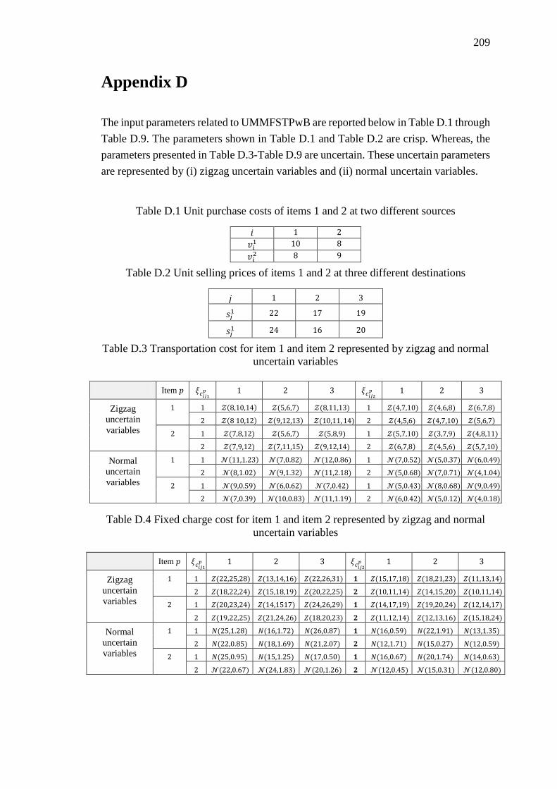
209

Appendix D

The input parameters related to UMMFSTPwB are reported below in Table D.1 through

Table D.9. The parameters shown in Table D.1 and Table D.2 are crisp. Whereas, the

parameters presented in Table D.3-Table D.9 are uncertain. These uncertain parameters

are represented by (i) zigzag uncertain variables and (ii) normal uncertain variables.

Table D.1 Unit purchase costs of items 1 and 2 at two different sources

𝑖 1 2

𝑣𝑖1 10 8

𝑣𝑖2 8 9

Table D.2 Unit selling prices of items 1 and 2 at three different destinations

𝑗 1 2 3

𝑠𝑗1 22 17 19

𝑠𝑗1 24 16 20

Table D.3 Transportation cost for item 1 and item 2 represented by zigzag and normal

uncertain variables

Table D.4 Fixed charge cost for item 1 and item 2 represented by zigzag and normal

uncertain variables

Item 𝑝 𝜉𝑐𝑖𝑗1𝑝 1 2 3 𝜉𝑐𝑖𝑗2

𝑝 1 2 3

Zigzag

uncertain

variables

1 1 𝒵(8,10,14) 𝒵(5,6,7) 𝒵(8,11,13) 1 𝒵(4,7,10) 𝒵(4,6,8) 𝒵(6,7,8)

2 𝒵(8 10,12) 𝒵(9,12,13) 𝒵(10,11, 14) 2 𝒵(4,5,6) 𝒵(4,7,10) 𝒵(5,6,7)

2 1 𝒵(7,8,12) 𝒵(5,6,7) 𝒵(5,8,9) 1 𝒵(5,7,10) 𝒵(3,7,9) 𝒵(4,8,11)

2 𝒵(7,9,12) 𝒵(7,11,15) 𝒵(9,12,14) 2 𝒵(6,7,8) 𝒵(4,5,6) 𝒵(5,7,10)

Normal

uncertain

variables

1 1 𝒩(11,1.23) 𝒩(7,0.82) 𝒩(12,0.86) 1 𝒩(7,0.52) 𝒩(5,0.37) 𝒩(6,0.49)

2 𝒩(8,1.02) 𝒩(9,1.32) 𝒩(11,2.18) 2 𝒩(5,0.68) 𝒩(7,0.71) 𝒩(4,1.04)

2 1 𝒩(9,0.59) 𝒩(6,0.62) 𝒩(7,0.42) 1 𝒩(5,0.43) 𝒩(8,0.68) 𝒩(9,0.49)

2 𝒩(7,0.39) 𝒩(10,0.83) 𝒩(11,1.19) 2 𝒩(6,0.42) 𝒩(5,0.12) 𝒩(4,0.18)

Item 𝑝 𝜉𝑐𝑖𝑗1𝑝 1 2 3 𝜉𝑐𝑖𝑗2

𝑝 1 2 3

Zigzag

uncertain

variables

1 1 𝑍(22,25,28) 𝑍(13,14,16) 𝑍(22,26,31) 𝟏 𝑍(15,17,18) 𝑍(18,21,23) 𝑍(11,13,14)

2 𝑍(18,22,24) 𝑍(15,18,19) 𝑍(20,22,25) 𝟐 𝑍(10,11,14) 𝑍(14,15,20) 𝑍(10,11,14)

2 1 𝑍(20,23,24) 𝑍(14,1517) 𝑍(24,26,29) 𝟏 𝑍(14,17,19) 𝑍(19,20,24) 𝑍(12,14,17)

2 𝑍(19,22,25) 𝑍(21,24,26) 𝑍(18,20,23) 𝟐 𝑍(11,12,14) 𝑍(12,13,16) 𝑍(15,18,24)

Normal

uncertain

variables

1 1 𝑁(25,1.28) 𝑁(16,1.72) 𝑁(26,0.87) 𝟏 𝑁(16,0.59) 𝑁(22,1.91) 𝑁(13,1.35)

2 𝑁(22,0.85) 𝑁(18,1.69) 𝑁(21,2.07) 𝟐 𝑁(12,1.71) 𝑁(15,0.27) 𝑁(12,0.59)

2 1 𝑁(25,0.95) 𝑁(15,1.25) 𝑁(17,0.50) 𝟏 𝑁(16,0.67) 𝑁(20,1.74) 𝑁(14,0.63)

2 𝒩(22,0.67) 𝒩(24,1.83) 𝒩(20,1.26) 𝟐 𝒩(12,0.45) 𝒩(15,0.31) 𝒩(12,0.80)

User

Text Box

210

Table D.6 Available amounts of item 1 and item 2 represented by zigzag and normal

uncertain variables

𝑖 1 2 𝑖 1 2

Zigzag

uncertain

variables

𝜉𝑎𝑖1 𝒵(31, 32, 35) 𝒵(34, 37, 41) 𝜉𝑎𝑖

2 𝒵(25, 26, 27) 𝒵(26, 29, 31)

Normal

uncertain

variables

𝜉𝑎𝑖1 𝒩(32,1.57) 𝒩(35,0.87) 𝜉𝑎𝑖

2 𝒩(25,1.73) 𝒩(28,0.47)

Tab

le D

.5 T

ransp

ort

atio

n t

ime

for

item

1 a

nd i

tem

2 r

epre

sente

d b

y z

igza

g a

nd n

orm

al u

nce

rtai

n v

aria

ble

s

It

em

𝑝

𝜉 𝑐𝑖𝑗1

𝑝

1

2

3

𝜉 𝑐𝑖𝑗2

𝑝

1

2

3

Zig

zag

un

cert

ain

var

iab

les

1

1

𝒵(12.0,14.0,15.0)

𝒵(6.7,8.6.2,11.2)

𝒵(9.5,11.2,12.1)

1

𝒵(8.2,9.4,10.5

) 𝒵(10.2,12.4,14.7)

𝒵(8.4,12.8,14.8)

2

𝒵 (

8.0

,9.0

,11.0

) 𝒵(12.2,14.6,16.3)

𝒵(11.9,14.4,17.2)

2

𝒵(6.8,7.8,10.4)

𝒵 (11.2,12.1,15.8)

𝒵(10.2,13.9,14.1)

2

1

𝒵(12.1,15.4,18.7)

𝒵(8.1,13.2,14.5)

𝒵(10.0,11.8,13.1)

1

𝒵(10.0,14.1,17.4)

𝒵(7.0,7.5,8.5)

𝒵(10.2,13.6,14.2)

2

𝒵(11.9,13.2,17.4

) 𝒵(10.0,12.0,14.0)

𝒵(10.0,13.7,15.0)

2

𝒵(9.0,11.0,13.5)

𝒵(8.0,10.5,12.0)

𝒵(13.0,14.6,16.0)

No

rmal

un

cert

ain

var

iab

les

1

1

𝒩(14.0,0.27)

𝒩(9

.2,0

.53

) 𝒩(11.7,0.49)

1

𝒩(8.6,1.2)

𝒩(12.2,0.6)

𝒩(11.2,1.6)

2

𝒩 (

11.6

,1.2

1)

𝒩(12.0,0.14

) 𝒩(14.4,0.75)

2

𝒩(12.2,1.0)

𝒩 (9.8,0.4)

𝒩(9.0,1.17)

2

1

𝒩(14.4,0.70)

𝒩(9.0,0.8)

𝒩(13.2,1.03)

1

𝒩(14.0,1.44)

𝒩(10.7,0.70)

𝒩(13.6,1.27)

2

𝒩(13.2,0.40)

𝒩(11.6,1.41)

𝒩(13.2,0.25)

2

𝒩(11.2,0.79)

𝒩(12.4,1.59)

𝒩(10.0,0.75)

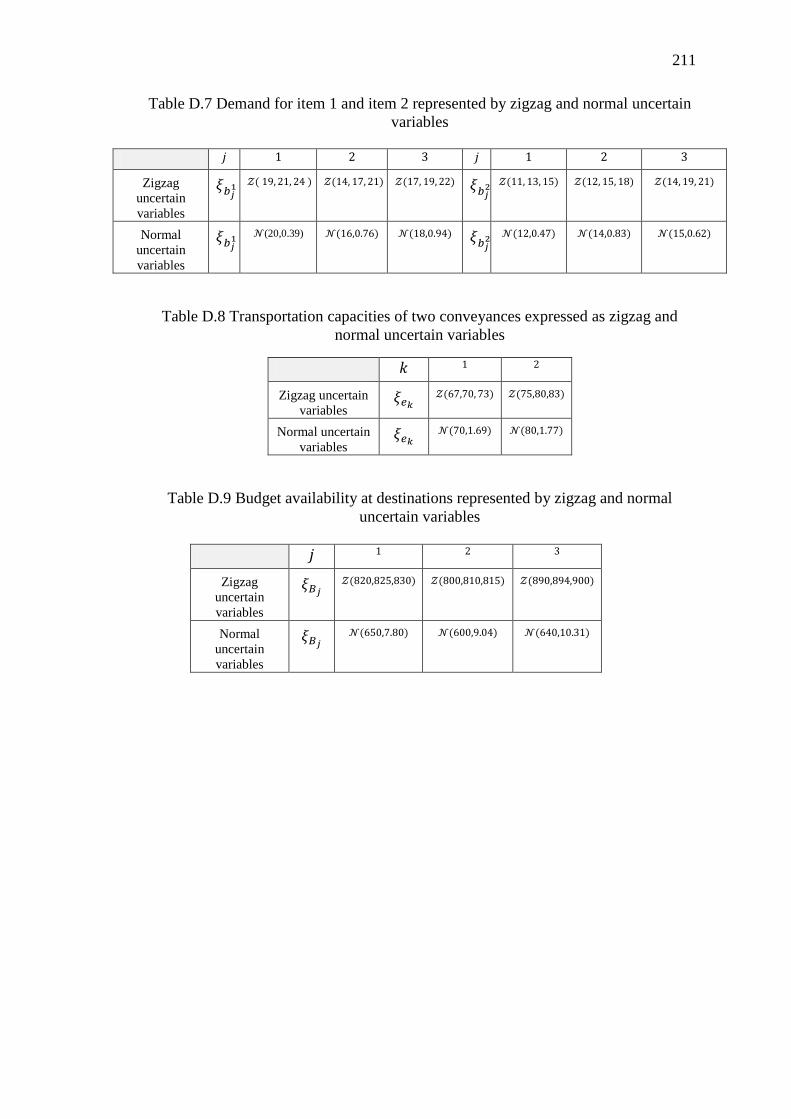
211

Table D.7 Demand for item 1 and item 2 represented by zigzag and normal uncertain

variables

Table D.8 Transportation capacities of two conveyances expressed as zigzag and

normal uncertain variables

𝑘 1 2

Zigzag uncertain

variables 𝜉𝑒𝑘 𝒵(67,70, 73) 𝒵(75,80,83)

Normal uncertain

variables 𝜉𝑒𝑘 𝒩(70,1.69) 𝒩(80,1.77)

Table D.9 Budget availability at destinations represented by zigzag and normal

uncertain variables

𝑗 1 2 3 𝑗 1 2 3

Zigzag

uncertain

variables

𝜉𝑏𝑗1

𝒵( 19, 21, 24 ) 𝒵(14, 17, 21) 𝒵(17, 19, 22) 𝜉𝑏𝑗2 𝒵(11, 13, 15) 𝒵(12, 15, 18) 𝒵(14, 19, 21)

Normal

uncertain

variables

𝜉𝑏𝑗1 𝒩(20,0.39) 𝒩(16,0.76) 𝒩(18,0.94) 𝜉𝑏𝑗

2 𝒩(12,0.47) 𝒩(14,0.83) 𝒩(15,0.62)

𝑗 1 2 3

Zigzag

uncertain

variables

𝜉𝐵𝑗 𝒵(820,825,830) 𝒵(800,810,815) 𝒵(890,894,900)

Normal

uncertain

variables

𝜉𝐵𝑗 𝒩(650,7.80) 𝒩(600,9.04) 𝒩(640,10.31)

212

User

Text Box

213

Appendix E

Data Tables for Input Parameters

The rough fuzzy input parameters related to the 𝑊 as shown in Fig. 6.6, are reported

below in the following tables.

Table E.1 The rough fuzzy linear weights representing the possible costs to the

company while providing the air service between a pair of cities

Edges Rough fuzzy linear weights Edges Rough fuzzy linear weights

𝑒1 [𝜉, 𝜉 + 1][𝜉 − 1, 𝜉 + 2]

𝜉 = (25, 26.5, 27.2) 𝑒11 [𝜉, 𝜉 + 0.8][𝜉 − 1, 𝜉 + 1.2]

𝜉 = (34.2, 36, 37.2)

𝑒2 [𝜉, 𝜉 + 2][𝜉 − 0.7, 𝜉 + 2.5]

𝜉 = (26.1, 28.3, 29.2) 𝑒12 [𝜉, 𝜉 + 1][𝜉 − 1, 𝜉 + 1.5]

𝜉 = (31.2, 32.7, 33.5)

𝑒3 [𝜉, 𝜉 + 1.2][𝜉 − 0.5, 𝜉 + 1.9]

𝜉 = (30.7,32.8, 34) 𝑒13 [𝜉, 𝜉 + 0.2][𝜉 − 0.2, 𝜉 + 1.4]

𝜉 = (36.1,37.2, 37.9)

𝑒4 [𝜉, 𝜉 + 1.5][𝜉 − 2, 𝜉 + 2.1]

𝜉 = (28.4, 29.7, 30.2) 𝑒14 [𝜉, 𝜉 + 0.5][𝜉 − 1.2, 𝜉 + 1.3]

𝜉 = (29.5, 31.4, 32.6)

𝑒5 [𝜉, 𝜉 + 1.7][𝜉 − 1.8, 𝜉 + 2.3]

𝜉 = (26.1, 28.9, 31.1) 𝑒15 [𝜉, 𝜉 + 1.2][𝜉 − 1.3, 𝜉 + 1.4]

𝜉 = (28.4, 29.3, 31.2)

𝑒6 [𝜉, 𝜉 + 1][𝜉 − 0.3, 𝜉 + 1.5]

𝜉 = (31.6, 34.5, 35.2) 𝑒16 [𝜉, 𝜉 + 1.2][𝜉 − 1.2, 𝜉 + 1.7]

𝜉 = (31.1, 33.6, 35)

𝑒7 [𝜉, 𝜉 + 0.7][𝜉 − 1, 𝜉 + 1.6]

𝜉 = (32.4, 33, 34.1) 𝑒17 [𝜉, 𝜉 + 1.7][𝜉 − 1, 𝜉 + 1.9]

𝜉 = (33.2, 35.8, 36.4)

𝑒8 [𝜉, 𝜉 + 0.7][𝜉 − 1, 𝜉 + 1.4]

𝜉 = (28.2, 29, 30.4) 𝑒18 [𝜉, 𝜉 + 1.2][𝜉 − 0.8, 𝜉 + 1.4]

𝜉 = (31.6, 32.7, 34.5)

𝑒9 [𝜉, 𝜉 + 0.2][𝜉 − 1, 𝜉 + 2]

𝜉 = (41.6, 43.5, 45.4) 𝑒19 [𝜉, 𝜉 + 1.2][𝜉 − 1, 𝜉 + 2]

𝜉 = (29.1, 30.9, 32.5)

𝑒10 [𝜉, 𝜉 + 0.9][𝜉 − 1.2, 𝜉 + 2]

𝜉 = (36.4, 37.2, 38.4) − − −−

User

Text Box

214

Table E.2 The rough fuzzy quadratic weights of a pair of adjacent edges representing

the possible discount on the total flight fare of two consecutive flights


𝑒1𝑒2 [𝜉, 𝜉 + 0.3][𝜉 − 1, 𝜉 + 1.7]

𝜉 = (10.8, 11.5, 12.9)

𝑒3𝑒4 [𝜉, 𝜉 + 0.6][𝜉 − 0.9, 𝜉 + 1.8]

𝜉 = (11.4, 12.4, 14.6)

𝑒1𝑒3 [𝜉, 𝜉 + 0.7][𝜉 − 1.2, 𝜉 + 1.2]

𝜉 = (12.1, 13.7, 14.5)

𝑒4𝑒7 [𝜉, 𝜉 + 0.2][𝜉 − 0.9, 𝜉 + 1.3]

𝜉 = (11.5, 12.8, 14.9)

𝑒2𝑒3 [𝜉, 𝜉 + 0.2][𝜉 − 0.9, 𝜉 + 1.7]

𝜉 = (11.7,12.8, 14.2)

𝑒4𝑒9 [𝜉, 𝜉 + 0.7][𝜉 − 0.8, 𝜉 + 1.6]

𝜉 = (11.5, 14.8, 15.7)

𝑒1𝑒4 [𝜉, 𝜉 + 1.2][𝜉 − 1.1, 𝜉 + 1.5]

𝜉 = (10.5, 11.3, 12.2)

𝑒4𝑒10 [𝜉, 𝜉 + 0.2][𝜉 − 0.7, 𝜉 + 1.7]

𝜉 = (12.7, 14.6, 15.2)

𝑒1𝑒5 [𝜉, 𝜉 + 1.1][𝜉 − 1.5, 𝜉 + 2.1]

𝜉 = (10.6, 11.5, 13.2)

𝑒7𝑒9 [𝜉, 𝜉 + 0.6][𝜉 − 0.9, 𝜉 + 1.9]

𝜉 = (14.2, 15.6, 16.2)

𝑒1𝑒6 [𝜉, 𝜉 + 0.3][𝜉 − 1, 𝜉 + 1.7]

𝜉 = (11.6, 14.5, 15.2)

𝑒7𝑒10 [𝜉, 𝜉 + 1][𝜉 − 1.2, 𝜉 + 1.4]

𝜉 = (13.2, 14.6, 15.7)

𝑒4𝑒5 [𝜉, 𝜉 + 1.1][𝜉 − 1.7, 𝜉 + 1.5]

𝜉 = (10.4, 11.7, 13.1)

𝑒9𝑒10 [𝜉, 𝜉 + 1][𝜉 − 1.5, 𝜉 + 1.7]

𝜉 = (14.2, 15.9, 17.2)

𝑒4𝑒6 [𝜉, 𝜉 + 0.3][𝜉 − 1, 𝜉 + 1.4]

𝜉 = (11.5, 12.8 ,14.4)

𝑒8𝑒9 [𝜉, 𝜉 + 0.2][𝜉 − 0.2, 𝜉 + 1.3]

𝜉 = (12.7,14.2, 15.9)

𝑒5𝑒6 [𝜉, 𝜉 + 0.8][𝜉 − 1, 𝜉 + 1.7]

𝜉 = (11.6, 12.5, 14.8)

𝑒8𝑒11 [𝜉, 𝜉 + 0.6][𝜉 − 0.8, 𝜉 + 1.7]

𝜉 = (12.7,13.9, 15.7)

𝑒2𝑒7 [𝜉, 𝜉 + 0.7][𝜉 − 1.4, 𝜉 + 1.5]

𝜉 = (10.7, 12.7, 13.6)

𝑒8𝑒12 [𝜉, 𝜉 + 0.4][𝜉 − 0.9, 𝜉 + 1.3]

𝜉 = (10.7,12.9, 14.6)

𝑒2𝑒8 [𝜉, 𝜉 + 0.5][𝜉 − 0.9, 𝜉 + 1.2]

𝜉 = (10.5, 12.4, 14.8)

𝑒9𝑒11 [𝜉, 𝜉 + 0.2][𝜉 − 1.3, 𝜉 + 1]

𝜉 = (12.7,14.9, 16.9)

𝑒7𝑒8 [𝜉, 𝜉 + 0.2][𝜉 − 0.8, 𝜉 + 1.3]

𝜉 = (12.5, 14.4, 15.1)

𝑒9𝑒12 [𝜉, 𝜉 + 1.5][𝜉 − 0.7, 𝜉 + 1.7]

𝜉 = (14.2, 15.8, 17.4)

𝑒3𝑒7 [𝜉, 𝜉 + 0.7][𝜉 − 0.2, 𝜉 + 1.6]

𝜉 = (12.1, 13.4, 14.3)

𝑒11𝑒12 [𝜉, 𝜉 + 0.5][𝜉 − 0.8, 𝜉 + 1.2]

𝜉 = (12.6, 13.7, 14.5)

𝑒3𝑒9 [𝜉, 𝜉 + 0.6][𝜉 − 0.5, 𝜉 + 1.7]

𝜉 = (13.1, 15.4, 16.7)

𝑒5𝑒10 [𝜉, 𝜉 + 1.1][𝜉 − 1.6, 𝜉 + 1.8]

𝜉 = (12.1, 13.9, 14.9)

𝑒3𝑒10 [𝜉, 𝜉 + 0.3][𝜉 − 0.8, 𝜉 + 1.6]

𝜉 = (12.1, 14.4, 15.8)

𝑒5𝑒11 [𝜉, 𝜉 + 0.1][𝜉 − 0.6, 𝜉 + 0.9]

𝜉 = (10.1, 12.7, 14.1)

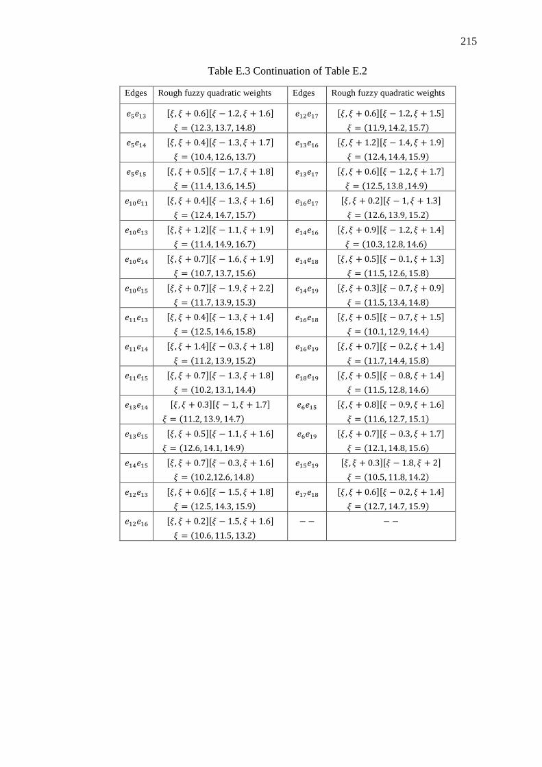
215

Table E.3 Continuation of Table E.2


𝑒5𝑒13 [𝜉, 𝜉 + 0.6][𝜉 − 1.2, 𝜉 + 1.6]

𝜉 = (12.3, 13.7, 14.8)

𝑒12𝑒17 [𝜉, 𝜉 + 0.6][𝜉 − 1.2, 𝜉 + 1.5]

𝜉 = (11.9, 14.2, 15.7)

𝑒5𝑒14 [𝜉, 𝜉 + 0.4][𝜉 − 1.3, 𝜉 + 1.7]

𝜉 = (10.4, 12.6, 13.7)

𝑒13𝑒16 [𝜉, 𝜉 + 1.2][𝜉 − 1.4, 𝜉 + 1.9]

𝜉 = (12.4, 14.4, 15.9)

𝑒5𝑒15 [𝜉, 𝜉 + 0.5][𝜉 − 1.7, 𝜉 + 1.8]

𝜉 = (11.4, 13.6, 14.5)

𝑒13𝑒17 [𝜉, 𝜉 + 0.6][𝜉 − 1.2, 𝜉 + 1.7]

𝜉 = (12.5, 13.8 ,14.9)

𝑒10𝑒11 [𝜉, 𝜉 + 0.4][𝜉 − 1.3, 𝜉 + 1.6]

𝜉 = (12.4, 14.7, 15.7)

𝑒16𝑒17 [𝜉, 𝜉 + 0.2][𝜉 − 1, 𝜉 + 1.3]

𝜉 = (12.6, 13.9, 15.2)

𝑒10𝑒13 [𝜉, 𝜉 + 1.2][𝜉 − 1.1, 𝜉 + 1.9]

𝜉 = (11.4, 14.9, 16.7)

𝑒14𝑒16 [𝜉, 𝜉 + 0.9][𝜉 − 1.2, 𝜉 + 1.4]

𝜉 = (10.3, 12.8, 14.6)

𝑒10𝑒14 [𝜉, 𝜉 + 0.7][𝜉 − 1.6, 𝜉 + 1.9]

𝜉 = (10.7, 13.7, 15.6)

𝑒14𝑒18 [𝜉, 𝜉 + 0.5][𝜉 − 0.1, 𝜉 + 1.3]

𝜉 = (11.5, 12.6, 15.8)

𝑒10𝑒15 [𝜉, 𝜉 + 0.7][𝜉 − 1.9, 𝜉 + 2.2]

𝜉 = (11.7, 13.9, 15.3)

𝑒14𝑒19 [𝜉, 𝜉 + 0.3][𝜉 − 0.7, 𝜉 + 0.9]

𝜉 = (11.5, 13.4, 14.8)

𝑒11𝑒13 [𝜉, 𝜉 + 0.4][𝜉 − 1.3, 𝜉 + 1.4]

𝜉 = (12.5, 14.6, 15.8)

𝑒16𝑒18 [𝜉, 𝜉 + 0.5][𝜉 − 0.7, 𝜉 + 1.5]

𝜉 = (10.1, 12.9, 14.4)

𝑒11𝑒14 [𝜉, 𝜉 + 1.4][𝜉 − 0.3, 𝜉 + 1.8]

𝜉 = (11.2, 13.9, 15.2)

𝑒16𝑒19 [𝜉, 𝜉 + 0.7][𝜉 − 0.2, 𝜉 + 1.4]

𝜉 = (11.7, 14.4, 15.8)

𝑒11𝑒15 [𝜉, 𝜉 + 0.7][𝜉 − 1.3, 𝜉 + 1.8]

𝜉 = (10.2, 13.1, 14.4)

𝑒18𝑒19 [𝜉, 𝜉 + 0.5][𝜉 − 0.8, 𝜉 + 1.4]

𝜉 = (11.5, 12.8, 14.6)

𝑒13𝑒14 [𝜉, 𝜉 + 0.3][𝜉 − 1, 𝜉 + 1.7]

𝜉 = (11.2, 13.9, 14.7)

𝑒6𝑒15 [𝜉, 𝜉 + 0.8][𝜉 − 0.9, 𝜉 + 1.6]

𝜉 = (11.6, 12.7, 15.1)

𝑒13𝑒15 [𝜉, 𝜉 + 0.5][𝜉 − 1.1, 𝜉 + 1.6]

𝜉 = (12.6, 14.1, 14.9)

𝑒6𝑒19 [𝜉, 𝜉 + 0.7][𝜉 − 0.3, 𝜉 + 1.7]

𝜉 = (12.1, 14.8, 15.6)

𝑒14𝑒15 [𝜉, 𝜉 + 0.7][𝜉 − 0.3, 𝜉 + 1.6]

𝜉 = (10.2,12.6, 14.8)

𝑒15𝑒19 [𝜉, 𝜉 + 0.3][𝜉 − 1.8, 𝜉 + 2]

𝜉 = (10.5, 11.8, 14.2)

𝑒12𝑒13 [𝜉, 𝜉 + 0.6][𝜉 − 1.5, 𝜉 + 1.8]

𝜉 = (12.5, 14.3, 15.9)

𝑒17𝑒18 [𝜉, 𝜉 + 0.6][𝜉 − 0.2, 𝜉 + 1.4]

𝜉 = (12.7, 14.7, 15.9)

𝑒12𝑒16 [𝜉, 𝜉 + 0.2][𝜉 − 1.5, 𝜉 + 1.6]

𝜉 = (10.6, 11.5, 13.2)

−− − −

216

User

Text Box

217

References Adlakha V., Kowalski K. (2003) A simple heuristic for solving small fixed-charge

transportation problem. Omega 31 (3): 205-211.

Agarwal P.K., Edelsbrunner H., Schwarzkopf O., Welzl E. (1991) Euclidean minimum

spanning trees and bi-chromatic closest pairs. Discrete & Computational Geometry 6

(3): 407–422.

Aggarwal S., Gupta C. (2016) Solving intuitionistic fuzzy solid transportation problem

via new ranking method based on signed distance. International Journal of

Uncertainty, Fuzziness and Knowledge-Based Systems 24 (4): 483-501.

Ahuja R.K., Orlin J.B. (1989) A fast and simple algorithm for the maximum flow

problem. Operations Research 37 (5): 748-759.

Ahuja R.K., Magnanti T.L., Orlin J.B. (1993) Network flows: Theory, algorithms, and

applications. Prentice-Hall, Upper Saddle River, NJ.

Alefeld G., Herzberger J. (1983) Introduction to interval computations. Academic

Press, New York.

Aliev R. A., Pedrycz W., Guirimov B., Aliev R. R., Ilhan U., Babagil M., Mammadli

S. (2011) Type-2 fuzzy neural networks with fuzzy clustering and differential evolution

optimization. Information Sciences 181 (9): 1591–1608.

Ammar E.E., Youness E.A. (2005) Study on multi-objective transportation problem

with fuzzy numbers. Applied Mathematics and Computation 166 (2): 241-253.

Andersen K.A., Jörnsten K., Lind M. (1996) On bi-criterion minimal spanning trees:

An approximation. Computers & Operations. Research 23 (12): 1171–1182.

Aneja Y.P., Nair K.P.K. (1979) Bi-criteria transportation problem. Management

Science 25 (1): 73-78.

Anusuya V., Sathya R. (2014) A new approach for solving type-2 fuzzy shortest path

problem. Annals of Pure and Applied Mathematics 8 (1): 83-92.

Appa G.M. (1973) The transportation problem and its variants. Journal of the

Operational Research Society 24 (1): 79-99.

Arsham H., Kahn A.B. (1989) A simplex-type algorithm for general transportation

problems: An alternative to stepping-stone. Journal of the Operational Research

Society 40 (6): 581-590.

Assad A., Xu W. (1992) The quadratic minimum spanning tree problem. Naval

Research Logistics 39 (3): 399-417.

Altassan K.M., EI-Sherbiny M.M., Abid A.D. (2014) Artificial immune algorithm for

solving fixed charge transportation problem. Applied Mathematics Information

Sciences 8 (2): 751-759.

User

Text Box

218

Baidya A., Bera U.K. (2014) An interval valued solid transportation problem with

budget constraint in different interval approaches. Journal of Transportation Security

7 (2): 147–155.

Barr R.S., Glover F., Klingman D. (1981) A new optimization method for large scale

fixed charge transportation problems. Operations Research 29 (3): 448–463.

Bellman R. (1958) On a routing problem. Quarterly of Applied Mathematics 16 (1): 87-

90.

Bellman R.E., Zadeh L.A. (1970) Decision making in a fuzzy environment.

Management Science 17 (4): 141-164.

Bhatia H.L. (1981) Indefinite quadratic solid transportation problem. Journal of

Information Optimization Sciences 2 (3): 297-303.

Bhatia H.L., Swarup K., Puri M.C. (1976) Time minimizing solid transportation

problem. Mathematische Operationsforschung Statistik 7 (3): 395-403.

Bilgen B. (2010) Application of fuzzy mathematical programming approach to the

production allocation and distribution supply chain network problem. Expert Systems

with Applications 37 (6): 4488–4495.

Bit A.K., Biswal M.P., Alam S.S. (1993) Fuzzy programming approach to multi-

objective solid transportation problem. Fuzzy Sets and Systems 57 (2): 183–194.

Borüvka O. (1926) O jistém problem minimálním. Práce Moravské Přírodovĕdecké

Společnosti III (3): 37-58.

Buson E., Roberti R., Toth P. (2014) A reduced-cost iterated local search heuristic for

the fixed-charge transportation problem. Operations Research 62 (5): 1095-1106.

Cabot A.V., Erenguc S.S. (1984) Some branch and bound procedures for fixed cost

transportation problems. Naval Research Logistics Quarterly 31 (1): 145–154.

Cabot A.V., Erenguc S.S. (1986) Improved penalties for fixed cost linear programs

using Lagrangean relaxation. Management Science 32 (1): 856–869.

Carey M., Henrickson C. (1986) Bounds on expected performance of networks with

links subject to failure. Networks 14 (3): 439-456.

Cascone A., Marigo A., Piccoli B., Rarità L. (2010) Decentralized optimal routing for

packets flow on data networks. Discrete and Continuous Dynamical Systems - Series B

(DCDS-B) 13 (1): 59-78.

Chakraborty D., Jana D.K., Roy T.K. (2014) A new approach to solve intuitionistic

fuzzy optimization problem using possibility, necessity, and credibility measures.

International Journal of Engineering Mathematics 2014, Article ID 593185, 12 pages

doi: 10.1155/2014/593185.

Chanas S., Kołodziejczyk W. (1982) Maximum flow in a network with fuzzy arc

capacities. Fuzzy Sets and Systems 8 (2): 165-173.

219

Chanas S., Kołodziejczyk W. (1984) Real-valued flows in a network with fuzzy arc

capacities. Fuzzy Sets and Systems 13 (2): 139-151.

Chanas S., Kołodziejczyk W. (1986) Integer flows in network with fuzzy capacity

constraints. Networks 16 (1): 17-31.

Chanas S., Kołodziejczyk W., Machaj A. (1984) A fuzzy approach to the transportation

problem. Fuzzy Sets and Systems 13 (3): 211-221.

Chanas S., Kuchta D. (1996) A concept of the optimal solution of the transportation

problem with fuzzy cost coefficients. Fuzzy Sets and Systems 82 (3): 299-305.

Chandy K.M., Lo T. (1973) The capacitated minimum spanning tree. Networks 3: 173-

182.

Chang P.-T., Lee E.S. (1994) Ranking fuzzy sets based on the concept of existence.

Computers & Mathematics with Applications 27 (9-10): 1-21.

Chang P.-T., Lee E. S. (1999) Fuzzy decision networks and deconvolution. Computers

& Mathematics with Applications 37 (11): 53–63.

Charnes A., Cooper W.W. (1959) Chance-constrained programming. Management

Science 6 (1): 73–79.

Chen B. Y., Lam W. H. K., Sumalee A., Li, Z. (2012) Reliable shortest path finding in

stochastic networks with spatial correlated link travel times. International Journal of

Geographical information Science 26 (2): 365–386.

Chen L., Peng J., Zhang B. (2017) Uncertain goal programming models for bi-criteria

solid transportation problem. Applied Soft Computing 51: 49-59.

Chen L., Peng J., Zhang B., Rosyida I. (2016) Diversified models for portfolio selection

based on uncertain semivariance. International Journal of Systems Science 48 (3): 637-

648.

Chen P., Nie Y. (M.) (2013) Bi-criterion shortest path problem with a general

nonadditive cost. Transportation Research Part B: Methodological 57: 419–435.

Chen S.-M., Lee .L-W. (2010) Fuzzy multiple criteria hierarchical group decision

making based on interval type-2 fuzzy sets. IEEE Transactions on Systems, Man, and

Cybernetics - Part A: Systems and Humans 40 (5): 1120–1128.

Chen T.-Y. (2013) An interactive method for multiple criteria group decision analysis

based on interval type-2 fuzzy sets and its application to medical decision making.

Fuzzy Optimization and Decision Making 12 (3): 323–356.

Chen T.-Y. (2014) A PROMETHEE-based outranking method for multiple criteria

decision analysis with interval type-2 fuzzy sets. Soft Computing 18 (5): 923-940.

Cheng H., Huang W., Cai J. (2013) Solving a fully fuzzy linear programming problem

through compromise programming. Journal of Applied Mathematics 2013, Article ID

726296, 10 pages doi: 10.1155/2013/726296.

220

Cheng Y. (2015) Forward approximation and backward approximation in fuzzy rough

sets. Neurocomputing 148: 340-353

Clímaco J.C.N., Pascoal M.M.B. (2012) Multi-criteria path and tree problems:

discussion on exact algorithms and applications. International Transactions in

Operational Research 19 (1–2): 63–98.

Cordone R., Passeri G. (2012) Solving the minimum quadratic spanning tree problem.

Applied Mathematics and Computation 218 (23): 11597-11612.

Corley H.W., Moon I.D. (1985) Shortest paths in networks with vector weights. Journal

of Optimization Theory and Applications 46 (1): 79–86.

Cui Q., Sheng Y. (2013) Uncertain programming model for solid transportation

problem. Information 15 (3): 342-348.

Ćustić A., Zhang R., Punnen A.P. (2018) The quadratic minimum spanning tree

problem and its variations. Discrete Optimization 27: 73- 87.

Cutolo A., Nicola C.D., Manzo R., Rarità L. (2012) Optimal paths on urban networks

using travelling times prevision. Modelling and Simulation in Engineering 2012,

Article ID: 564168, 9 pages.

Dalman H. (2016) Uncertain programming model for multi-item solid transportation

problem. International Journal of Machine Learning and Cybernetics doi:

10.1007/s13042-016-0538-7.

Dantzig G.B. (1951) Application of the simplex method to a transportation problem.

In: Activity Analysis of Production and Allocation (T.C. Koopmans, ed.). John Wiley

& Sons, New York, pp. 359-373.

Darmann A., Pferschy U., Schauer J., Woeginger G.J. (2011) Paths, trees and matchings

under disjunctive constraints. Discrete Applied Mathematics 159 (16): 1726-1735.

Das A., Bera U.K., Maiti M. (2016) A profit maximizing solid transportation model

under rough interval approach. IEEE Transactions on Fuzzy Systems 25 (3): 485-498.

Das A., Bera U.K., Maiti M. (2017) Defuzzification and application of trapezoidal type-

2 fuzzy variables to green solid transportation problem. Soft Computing, doi:

10.1007/s00500-017-2491-0.

Das S.K., Goswami A., Alam S.S. (1999) Multi-objective transportation problem with

interval cost, source and destination parameters. European Journal of Operational

Research 117 (1): 100-112.

De Almeida T.A., Yamakami A., Takahashi M. T. (2005a) An evolutionary approach

to solve minimum spanning tree problem with fuzzy parameters. In: Proceedings of the

International Conference on Computational Intelligence for Modelling, Control and

Automation and International Conference on Intelligent Agents, Web Technologies and

Internet Commerce, CIMCA-IAWTIC'06, Vienna, pp. 203-208.

221

De Almeida T.A., Prado F.M.S., Souza V.N., Yamakami A., Takahashi M.T.(2005b)

A genetic algorithm to solve minimum spanning tree problem with fuzzy parameters

using possibility measure. In: Proceedings of the North American Fuzzy Information

Processing Society, NAFIPS 2005, Detroit, United States, pp. 627-632.

Deb K., Pratap A., Agarwal S., Meyarivan T. (2002) A fast and elitist multi-objective

genetic algorithm: NSGA-II. IEEE Transactions on Evolutionary Computation 6 (2):

182- 197.

Dembczyński K., Greco S., Słowiński R. (2009) Rough set approach to multiple criteria

classification with imprecise evaluations and assignments. European Journal of

Operational Research 198 (2): 626-636.

Dhamdhere, K., Ravi R., Singh M. (2005) On two-stage stochastic minimum spanning

trees. In: Integer Programming and Combinatorial Optimization, IPCO 2005 (M.

Jünger and V. Kaibel, eds.). Lecture Notes in Computer Science, Springer, Berlin,

Heidelberg, vol. 3509, pp. 321–334.

Deng Y., Chen Y., Zhang Y., Mahadevan S. (2012) Fuzzy Dijkstra algorithm for

shortest path problem under uncertain environment. Applied Soft Computing 12 (3):

1231-1237.

Dijkstra E.W. (1959) A note on two problems in connexion with graphs. Numerische

Mathematlk 1: 269-271.

Diker M. (2018) Textures and fuzzy unit operations in rough set theory: An approach

to fuzzy rough set models. Fuzzy Sets and Systems 336: 27-53

Ding S. (2015) The 𝛼-maximum flow model with uncertain capacities. Applied

Mathematical Modelling 39 (7): 2056-2063.

Dinic E.A. (1970) Algorithm for solution of a problem of maximum flow in networks

with power estimation. Soviet Math Doklady 11 (5): 1277-1280.

Di Puglia Pugliese L., Guerriero F., Santos J.L. (2015) Dynamic programming for

spanning tree problems: application to the multi-objective case. Optimization Letters 9

(3): 437–450.

Dou Y., Zhu L., Wang H.S. (2012) Solving the fuzzy shortest path problem using multi-

criteria decision method based on vague similarity measure. Applied Soft Computing

12 (6): 1621-1631.

Doulliez P. (1971) Probability distribution function for the capacity of a multi-terminal

network. RAIRO - Operations Research 5 (V1): 39-49.

Dreyfus S.E. (1969) An appraisal of some shortest-path algorithms. Operations

Research 17 (3): 395-412.

Dubois D., Prade H. (1980) Fuzzy sets and systems: Theory and applications. Academic

Press, New York.

222

Dubois D., Prade H. (1990) Rough fuzzy sets and fuzzy rough sets. International

Journal of General Systems 17 (2-3): 191–208.

Durillo J.J., Nebro A.J. (2011) jMetal: a java framework for multi-objective

optimization. Advances in Engineering Software 42 (10): 760-771.

Dursun P. Bozdağ E. (2014) Chance-constrained programming models for constrained

shortest path problem with fuzzy parameters. Journal of Multiple-Valued Logic and

Soft Computing 22 (4-6): 599-618.

Ebrahimnejad A., Karimnejad Z., Alrezaamiri H. (2015) Particle swarm optimization

algorithm for solving shortest path problems with mixed fuzzy arc weights.

International Journal of Applied Decision Sciences 8 (2): 203-222.

Eckenrode R.T. (1965) Weighting multiple criteria. Management Science 12 (3): 180-

192.

Edmonds J., Karp R.M. (1972) Theoretical improvements in algorithmic efficiency for

network flow problems. Journal of the Association for Computing Machinery 19 (2):

248-264.

Ehrgott M. (2005) Multi-criteria optimization. Springer-Verlag, Berlin Heidelberg.

Enke D., Mehdiyev N. (2013) Type-2 fuzzy clustering and a type-2 fuzzy inference

neural network for the prediction of short-term interest rates. Procedia Computer

Science 20: 115-120.

Ericsson M., Resende M.G.C., Pardalos P.M. (2001) A genetic algorithm for the weight

setting problem in OSPF routing. Journal of Combinatorial Optimization 6 (3): 299–

333.

Eshelman L.J. (1991) The CHC adaptive search algorithm: How to have safe search

when engaging in in nontraditional genetic recombination. In: Foundations of Genetic

Algorithms (G.J.E. Rawlins, ed.). Elsevier, vol. 1, pp. 265-283.

Euler L. (1736) Solutio problematis ad geometriam situs pertinentis. Commentarii

academiae scientiarum Petropolitanae 8: 128-140.

Evans J.R. (1976) Maximum flow in probabilistic graphs‐the discrete case. Networks 6

(2): 161:183.

Feng L., Wang G.-Y., Li X.‐X. (2010) Knowledge acquisition in vague objective

information systems based on rough sets. Expert Systems 27 (2): 129-142

Figueroa-García J.C (2012) A general model for linear programming with interval type-

2 fuzzy technological coefficients. In: Proceedings of the IEEE Annual Meeting of the

North American Fuzzy Information Processing Society, NAFIPS ’12, Berkeley, pp. 1–

4.

Figueroa-García J.C., Hernández G. (2014) A method for solving linear programming

models with interval type-2 fuzzy constraints. Pesquisa Operacional 34 (1): 73–89.

223

Fishman G.S. (1987) The distribution of maximum flow with applications to multistate

reliability systems. Operations Research 35 (4): 607-618.

Floyd R. W. (1962) Algorithm 97: Shortest path. Communications of the Association

for Computing Machinery 5 (6): 345.

Ford L.R., Fulkerson D.R. (1956) Maximal flow through a network. Canadian Journal

of Mathematics 8 (3): 399-404.

Ford L.R., Fulkerson D.R. (1962) Flows in networks. Princeton University Press,

Princeton, NJ.

Frank H., Hakimi S.L. (1965) Probabilistic flows through a communication network.

IEEE Transactions on Circuit Theory 12 (3): 413-414.

Frieze A. M. (1985) On the value of a random minimum spanning tree problem.

Discrete Applied Mathematics 10 (1): 47–56.

Fu L., Rilett L.R. (1998) Expected shortest paths in dynamic and stochastic traffic

networks. Transportation Research Part B: Methodological 32 (7): 499-516.

Fulkerson D.R., Dantzig G.B. (1955) Computations of maximum flow in networks.

Naval Research Logistics Quarterly 2 (4): 277-283.

Gabow H.N. (1977) Two algorithms for generating weighted spanning trees in order.

SIAM Journal on Computing 6 (1): 139–150.

Gabow H.N. (1985) Scaling algorithms for network problems. Journal of Computer

and System Sciences 31 (2): 148-168.

Gandibleux X, Beugnies F, Randriamasy S (2006) Martins’ algorithm revisited for

multi-objective shortest path problems with a MaxMin cost function. 4OR 4 (1): 47–

59.

Gao Y. (2011) Shortest path problem with uncertain arc lengths. Computers &

Mathematics with applications 62 (6): 2591-2600.

Gao J., Lu M. (2005) Fuzzy quadratic minimum spanning tree problem. Applied

Mathematics and Computation 164 (3): 773-788.

Gao S.P., Liu S.Y. (2004) Two-phase fuzzy algorithms for multi-objective

transportation problem. Journal of Fuzzy Mathematics 12 (1): 147-156.

Gao J., Yang X., Liu D. (2017) Uncertain Shapley value of coalitional game with

application to supply chain alliance. Applied Soft Computing 56: 551-556.

Gao J., Yao K. (2015) Some concepts and theorems of uncertain random process.

International Journal of Intelligent Systems 30 (1): 52-65.

Gao W., Zhang Q., Lu Z., Wu D., Du X. (2018) Modelling and application of fuzzy

adaptive minimum spanning tree in tourism agglomeration area division. Knowledge-

Based Systems 143: 317-326

224

Gao X., Jia L. (2017) Degree constrained minimum spanning tree problem with

uncertain edge weights. Applied Soft Computing 56: 580-588.

Gao X., Jia L., Kar S. (2017) Degree constrained minimum spanning tree problem of

uncertain random network. Journal of Ambient Intelligence and Humanized Computing

8 (5): 747-757.

Gao Y., Kar S. (2017) Uncertain solid transportation problem with product blending.

International Journal of Fuzzy Systems https://doi.org/10.1007/s40815-016-0282-x.

Garey M.R., Johnson D.S. (1990) Computers and intractability: A guide to the theory

of NP-completeness. W.H. Freeman & Co., New York, NY, USA.

Gass S.I. (1990) On solving the transportation problem. Journal of the Operational

Research Society 41 (4): 291-297.

Gembicki F.W. (1974) Vector optimization for control with performance and

parameter sensitivity indices. Ph.D. Dissertation, Case Western Reserve University,

Cleveland, OH.

Gen M., Altiparamk F., Lin L. (2006) A genetic algorithm for two-stage transportation

problem using priority-based encoding. OR Spectrum 28 (3): 337-354.

Gen M., Cheng R. (1997) Genetic algorithms and engineering design, 1st ed. Wiley,

New York.

Gen M., Cheng R., Lin L. (2008) Network models and optimization, 1st ed. Springer‐

Verlag, London.

Gen M., Cheng R., Wang D. (1997) Genetic algorithms for solving shortest path

problems. In: Proceedings of the IEEE International Conference on Evolutionary

Computation, ICEC’97, Indianapolis, IN, USA, pp. 488–493.

Gen M., Ida K., Li Y., Kubota E. (1995) Solving bi-criteria solid transportation problem

with fuzzy numbers by a genetic algorithm. Computers and Industrial Engineering 29

(1-4): 537-541.

Giri P.K., Maity M.K., Maiti M. (2015) Fully fuzzy fixed charge multi-item solid

transportation problem. Applied Soft Computing 27: 77–91.

Goldberg A.V., Tarjan R.E. (1986) A new approach to the maximum flow problem. In:

Proceedings of the 18th Annual ACM Symposium on the Theory of Computing,

STOC'86, Berkeley, pp. 136–146.

Graham R.L., Hell P. (1985) On the history of the minimum spanning tree problem.

IEEE Annals of the History of Computing 7 (1): 43–57.

Gu T., Xu Z. (2007) The symbolic algorithms for maximum flow in networks.

Computers & Operations Research 34 (3): 799-816.

Guo C., Gao J. (2017) Optimal dealer pricing under transaction uncertainty. Journal of

Intelligent Manufacturing 28 (3): 657-665.

225

Guo H., Wang X., Zhou S. (2015) A transportation problem with uncertain costs and

random supplies. International Journal of e-Navigation and Maritime Economy 2: 1-

11.

Gupta A., Warburton A. (1987) Approximation methods for multiple criteria travelling

salesman problems. In: Toward Interactive and Intelligent Decision Support Systems

(Y. Sawaragi, K. Inoue, H. Nakayama, eds.). Lecture Notes in Economics and

Mathematical Systems. Springer, Berlin, vol. 285, pp. 211-217.

Hachtel G.D., Somenzi F. (1997) A symbolic algorithm for maximum flow in 0-1

networks. Formal Methods in System Design 10 (2-3): 207–219.

Hadley G., Whitin T.M. (1963) Analysis of inventory systems. Prentice Hall.

Haley K.B. (1962) The solid transportation problem. Operational Research 10 (4): 448-

463.

Han L., Wang Y. (2005) A novel genetic algorithm for multi-criteria minimum

spanning tree problem. In: Computational Intelligence and Security, CIS 2005 (Y. Hao,

J. Liu, Y. Wang, Y.-M. Cheung, H. Yin, L. Jiao, J. Ma, Y.-C. Jiao, eds.). Lecture Notes

in Computer Science, Springer Berlin Heidelberg, Berlin, Heidelberg, vol. 3801, pp.

297-302.

Han S., Peng Z., Wang S. (2014) The maximum flow problem of uncertain network.

Information Sciences 265: 167-175.

Haimes Y.Y., Lasdon L.S., Wismer D.A. (1971) On a bi-criterion formulation of the

problems of integrated system identification and system optimization. IEEE

Transaction on Systems, Man, and Cybernetics 1 (3): 296-297.

Hall R. (1986) The fastest path through a network with random time-dependent travel

time. Transportation Science 20 (3): 182-188.

Hansen E. (1992) Global optimization using interval analysis. Marcel Dekker, New

York.

Hansen P. (1980) Bi-criterion path problems. In: Multiple Criteria Decision Making

Theory and Application (G. Fandel, T. Gal, eds.). Lecture notes in Economics and

Mathematical Systems, Springer, Berlin Heidelberg, vol. 177, pp. 109–127.

Harris R. (1998) Introduction to decision making. VirtualSalt,

http://www.virtualsalt.com/crebook5.htm.

Harris T. E., Ross F. S. (1955). Fundamentals of a method for evaluating rail net

capacities. Research Memorandum, AD Number: AD093458, Rand Corporation.

Hassanzadeh R., Mahdavi I., Mahdavi-Amiri N., Tajdin A. (2013) A genetic algorithm

for solving fuzzy shortest path problems with mixed fuzzy arc lengths. Mathematical

and Computer Modelling 57 (1–2): 84-99.

226

Hasuike T. (2010) Fuzzy random shortest path problem using conditional Value at Risk.

In: Proceedings of the International Conference on System Science and Engineering,

ICSSE 2010, Taipei, Taiwan, pp. 439-444.

Haugland D., Eleyat M., Hetland, M.L. (2011). The maximum flow problem with

minimum lot sizes. In: International Conference on Computational Logistics, ICCL

2011 (J.W. Böse, H. Hu, C. Jahn, X. Shi, R. Stahlbock, S. Voß, eds.). Lecture Notes in

Computer Science, Hamburg, Germany, vol. 6971, pp. 170–182.

Henig M.I. (1986) The shortest path problem with two objective functions. European

Journal of Operational Research 25 (2): 281-291.

Hernandes F., Lamata M.T., Verdegay J.L., Yamakami A. (2007a) The shortest path

problem on networks with fuzzy parameters. Fuzzy Sets and Systems 158 (14): 1561-

1570.

Hernandes F., Lamata M.T., Takahashi M.T. (2007b) An Algorithm for the fuzzy

maximum flow problem. In: IEEE International Fuzzy Systems Conference, FUZZ-

IEEE 2007, London, pp. 1-6.

Hirano S., Tsumoto S. (2005) Rough representation of a region of interest in medical

images. International Journal of Approximate Reasoning 40 (1-2): 23-34.

Hirsch W.M., Dantzig G.B. (1968) The fixed charge problem. Naval Research

Logistics Quarterly 15 (3): 413-424.

Hitchcock F.L. (1941) The distribution of product from several sources to numerous

localities. Journal of Mathematical Physics 20 (1-4): 224–230.

Holland H. J. (1975) Adaptation in natural and artificial systems. University of

Michigan Press, Ann Arbor, MI.

Huang X. (2007a) Chance-constrained programming models for capital budgeting with

NPV as fuzzy parameters. Journal of Computational and Applied Mathematics 198 (1):

149-159.

Huang X. (2007b) Optimal project selection with random fuzzy parameters.

International Journal of Production Economics 106 (2): 513–522.

Huang X. (2012) A risk index model for portfolio selection with returns subject to

experts’ estimations. Fuzzy Optimization and Decision Making 11 (4): 451–463.

Iori M., Martello S., Pretolani D. (2010) An aggregate label setting policy for the multi-

objective shortest path problem. European Journal of Operational Research 207 (3):

1489-1496.

Janiak A., Kasperski A. (2008) The minimum spanning tree problem with fuzzy costs.

Fuzzy Optimization and Decision Making 7 (2): 105–118.

Jarník V. (1930) O jistém problem minimálním. Práce Moravské Přírodovĕdecké

Společnosti IV (3): 57-63.

227

Ji X., Yang L., Shao Z. (2006) Chance-constrained maximum flow problem with fuzzy

arc capacities. In: International Conference on Intelligent Computing, ICIC 2006 (D.-

S. Huang, K. Li, G.W. Irwin, eds.). Lecture Notes in Computer Science, Springer,

Berlin, Heidelberg, vol. 4114, pp. 11–19.

Ji X., Iwamura K., Shao Z. (2007) New models for shortest path problem with fuzzy

arc lengths. Applied Mathematical Modelling 31 (2): 259-269.

Jian L., Xiaojing X., Kaiquan S. (2008) Rough similarity degree and rough close degree

in rough fuzzy sets and the applications. Journal of Systems Engineering and

Electronics 19 (5): 945-951.

Jiménez F., Verdegay J.L. (1998) Uncertain solid transportation problems. Fuzzy Sets

and Systems 100 (1–3): 45-57.

Jiménez F., Verdegay J. (1999) An evolutionary algorithm for interval solid

transportation problems. Evolutionary Computation 7 (1): 103-107.

Isermann H. (1979) The enumeration of all efficient solutions for a linear multi-

objective transportation problem. Naval Research Logistics Quarterly 26 (1): 123-139.

Ishii H., Shiode S., Nishida T., Namasuya Y. (1981) Stochastic spanning tree problem.

Discrete Applied Mathematics 3 (4): 263–273.

Ishii H., Matsutomi T. (1995) Confidence regional method of stochastic spanning tree

problem. Mathematical and Computer Modelling 22 (10): 77–82.

Itoh T., Ishii H. (1996) An approach based on necessity measure to the fuzzy spanning

tree problems. Journal of the Operations Research Society of Japan 39 (2): 247–257.

Jiménez F., Verdegay J.L. (1998) Uncertain solid transportation problems. Fuzzy Sets

and Systems 100 (1–3): 45-57.

Jiménez F., Verdegay J.L. (1999) Solving fuzzy solid transportation problems by an

evolutionary algorithm based parametric approach. European Journal of Operational

Research 117 (3): 485-510.

Jungnickel D. (1999) Graphs, Networks and Algorithms. Springer-Verlag, Berlin.

Karger D.R., Klein P.N., Tarjan R.E. (1995) A randomized linear-time algorithm to

find minimum spanning trees. Journal of the Association for Computing Machinery 42

(2): 321–328.

Karzanov A.V. (1974) Determining the maximal flow in a network by the method of

preflows. Soviet Math Doklady 15 (2): 434-437.

Katagiri H., Kato K., Hasuike T. (2012) A random fuzzy minimum spanning tree

problem through a possibility-based value at risk model. Expert Systems with

Applications 39 (12): 10639-10646.

Katagiri H., Mermri E.B., Sakawa M., Kato K. (2004) A study on fuzzy random

minimum spanning tree problems through possibilistic programming and the

228

expectation optimization model. In: Proceedings of the 47th IEEE International

Midwest Symposium on Circuits and Systems, Hiroshima, Japan, pp. III-49-III-52.

Kaufmann A., Gupta M.M. (1985) Introduction to fuzzy arithmetic: Theory and

applications. Van Nostrand Reinhold, New York.

Kaur A., Kumar A. (2012) A new approach for solving fuzzy transportation

problems using generalized trapezoidal fuzzy numbers. Applied Soft Computing 12

(3): 1201−1213.

Kennington J., Unger E. (1976) A new branch-and-bound algorithm for the fixed-

charge transportation problem. Management Science 22 (10): 1116–1126.

Keshavarz E., Khorram E. (2009) A fuzzy shortest path with the highest reliability.

Journal of Computational and Applied Mathematics 230 (1): 204-212.

Kim K., Roush F. (1982) Fuzzy flows on networks. Fuzzy Sets and Systems 8 (1): 35-

38.

Klein C.M. (1991) Fuzzy shortest paths. Fuzzy Sets and Systems 39 (1): 27-41.

Knuth D.E. (1977) A generalization of Dijkstra’s algorithm. Information Processing

Letters 6 (1): 1–5.

König D. (1936) Theorie der endlichen und unendlichen Graphen. Akademische

Verlagsgesellschaft, Leipzig.

Koopmans T.C. (1949) Optimum utilization of the transportation system.

Econometrica: Journal of the Econometric Society 17: 136-146.

Kostreva M.M., Wiecek M.M. (1993) Time dependency in multiple objective dynamic

programming. Journal of Mathematical Analysis and Applications 173 (1): 289–307.

Kowalski K., Lev B., Shen W., Tu Y. (2014) A fast and simple branching algorithm for

solving small scale fixed-charge transportation problem. Operations Research

Perspectives 1 (1): 1-5.

Kruskal Jr. J.B. (1956) On the shortest spanning subtree of a graph and traveling

salesman problem. In: Proceeding of the American Mathematical Society 7 (1): 48–50.

Kumar A., Kaur M. (2010) An algorithm for solving fuzzy maximal flow problems

using generalized trapezoidal fuzzy numbers. International Journal of Applied Science

and Engineering 8 (2): 109–118.

Kumar A., Kaur M. (2011) Solution of fuzzy maximal flow problems using fuzzy linear

programming. International Journal of Computational and Mathematical Sciences 5

(2): 62–67.

Kumar M.K., Sastry V.N. (2013) A new algorithm to compute Pareto-optimal paths in

a multi-objective fuzzy weighted network. Opsearch 50 (3): 297-318.

229

Kumar R., Jha S., Singh S. (2017) Shortest path problem in network with type-2

triangular fuzzy arc length. Journal of Applied Research on Industrial Engineering 4

(1): 1-7.

Kundu P., Kar S., Maiti M. (2013a) Some solid transportation models with crisp and

rough costs. International Journal of Mathematical and Computational Sciences 7 (1):

14-21.

Kundu P., Kar S., Maiti M. (2013b) Multi-objective solid transportation problems with

budget constraint in uncertain environment. International Journal of Systems Science

45 (8): 1668-1682.

Kundu P., Kar S., Maiti M. (2013c) Multi-objective multi-item solid transportation

problem in fuzzy environment. Applied Mathematical Modelling 37 (4): 2028-2038.

Kundu P., Kar S., Maiti M. (2014a) Fixed charge transportation problem with type-2

fuzzy variables. Information Sciences 255: 170-186.

Kundu P., Kar S., Maiti M. (2014b) A fuzzy MCDM method and an application to solid

transportation problem with mode preference. Soft Computing 18 (9): 1853-1864.

Kundu P., Kar S., Maiti M. (2017a) A fuzzy multi-criteria group decision making based

on ranking interval type-2 fuzzy variables and an application to transportation mode

selection problem. Soft Computing 21 (11): 3051–3062.

Kundu P., Kar M.B., Kar S., Pal T., Maiti M. (2017b) A solid transportation model with

product blending and parameters as rough variables. Soft Computing 21 (9): 2297–

2306.

Kwakernaak H. (1978) Fuzzy random variables—I. definitions and theorems.

Information Sciences 15 (1): 1–29.

Lamar B.W., Wallace C.A. (1997) Revised-modified penalties for fixed charge

transportation problems. Management Science 43 (10): 1431–1436.

Last M., Eyal S. (2005) A fuzzy-based lifetime extension of genetic algorithms. Fuzzy

Sets and Systems 149 (1): 131–147.

Le H., Gogne Z. (2010) Fuzzy linear programming with possibility and necessity

relation. In: Fuzzy Information and Engineering 2010 (B. Cao, G. Wang, S. Guo, S.

Chen, eds.). Advances in Intelligent and Soft Computing, Springer, Berlin, vol. 78, pp.

305–311.

Li T.-J., Zhang W.-X. (2008) Rough fuzzy approximations on two universes of

discourse. Information Sciences 178 (3): 892–906.

Li Y., Zou C.Y., Zhang S., Vai M.I. (2013) Research on multi-objective minimum

spanning tree algorithm based on ant algorithm. Research Journal of Applied Sciences,

Engineering and Technology 5 (21): 5051-5056.

230

Lin L., Gen M. (2007) A bi-criteria shortest path routing problems by hybrid genetic

algorithm in communication networks. 2007 IEEE Congress on Evolutionary

Computation, CEC 2007, Singapore, pp. 4577-4582.

Lin Y., Li Y., Wang C., Chen J. (2018) Attribute reduction for multi-label learning with

fuzzy rough set. Knowledge-Based Systems doi: 10.1016/j.knosys.2018.04.004.

Liou T.-S., Wang M.-J. J. (1992) Ranking fuzzy numbers with integral value. Fuzzy

Sets and Systems 50 (3): 247-255.

Liu B. (1997) Dependent-chance programming: A class of stochastic programming.

Computers and Mathematics with Applications 34 (12): 89-104.

Liu B. (2001) Random fuzzy variables and random fuzzy programming. Technical

Report.

Liu B. (2002) Theory and practice of uncertain programming, 1st ed. Springer-Verlag,

Berlin.

Liu B. (2004) Uncertainty theory: An introduction to its axiomatic foundation, 1st ed.

Springer-Verlag, Berlin.

Liu B. (2007) Uncertainty theory, 2nd edn. Springer-Verlag, Berlin.

Liu B. (2009) Some research problems in uncertainty theory. Journal of Uncertain

Systems 3 (1): 3-10.

Liu B. (2010) Uncertainty theory: A branch of mathematics for modeling human

uncertainty. Springer-Verlag, Berlin.

Liu B. (2012) Why is there a need for uncertainty theory? Journal of Uncertain System

6 (1): 3–10.

Liu B., Iwamura K. (1998) Chance-constrained programming with fuzzy parameters.

Fuzzy Sets and Systems 94 (2): 227-237.

Liu B., Liu Y.-K. (2002) Expected value of fuzzy variable and fuzzy expected value

models. IEEE Transactions on Fuzzy Systems 10 (4): 445–450.

Liu S.T., Kao C. (2004) Network Flow Problems with Fuzzy Arc Lengths. IEEE

Transactions on Systems, Man and Cybernetics 34(1): 765-769.

Liu Y.-K., Liu B. (2003) Expected value operator of random fuzzy variable and random

fuzzy expected value models. International Journal of Uncertainty, Fuzziness and

Knowledge-Based Systems 11 (2): 195-215.

Liu W., Yang C. (2007) Fuzzy random degree constrained minimum spanning tree

problem. International Journal of Uncertainty, Fuzziness and Knowledge-Based

Systems 15 (2): 107-115.

Liu L, Yang X, Mu H, Jiao Y (2008) The fuzzy fixed charge transportation problem

and genetic algorithm. In: Proceedings of the Fifth International Conference on Fuzzy

231

Systems and Knowledge Discovery, FSKD’08, IEEE Computer Society Washington,

DC, USA, pp. 208–212.

Liu L., Zhang B., Ma W. (2017) Uncertain programming models for fixed charge multi-

item solid transportation problem. Soft Computing doi: 10.1007/s00500-017-2718-0.

Liu P., Yang L., Wang L., Li S. (2014a) A solid transportation problem with type-2

fuzzy variables. Applied Soft Computing 24: 543–558.

Liu W., Yang C. (2007) Fuzzy random degree constrained minimum spanning tree


Systems 15 (2): 107-115.

Liu Y., Ha M. (2010) Expected value of function of uncertain variables. Journal of

Uncertain Systems 4 (3): 181-186.

Liu Y., Lin Y., Zhao H.-h. (2014b) Variable precision intuitionistic fuzzy rough set

model and applications based on conflict distance. Expert Systems 32 (2): 220-227

Liu Y.-K., Liu B (2000) Fuzzy random variables: A scalar expected value. Technical

Report.

Liu Z.Q., Liu Y.-K. (2010) Type-2 fuzzy variables and their arithmetic. Soft Computing

14 (7): 729–747.

Lotfi M.M., Tavakkoli-Moghaddam R. (2013) A genetic algorithm using priority-based

encoding with new operators for fixed charge transportation problems. Applied Soft

Computing 13 (5): 2711-2726.

Lozano M., Glover F., García-Martínez C., Rodríguez F.J., Martí R. (2013) Tabu search

with strategic oscillation for the quadratic minimum spanning tree. IIE Transactions 46

(4): 414-428

Mahapatra D.R., Roy S.K., Biswal M.P. (2010) Multi-objective stochastic

transportation problem involving log-normal. Journal of Physical Science 14: 63-76.

Mahdavi I., Nourifar R., Heidarzade A., Amiri N.M. (2009) A dynamic programming

approach for finding shortest chains in a fuzzy network. Applied Soft Computing 9 (2):

503-511.

Mahdavi I., Mahdavi-Amiri N., Nejati S. (2011) Algorithms for bi-objective shortest

path problems in fuzzy networks. Iranian Journal of Fuzzy Systems 8 (4): 9-37.

Maia S.M.D.M., Goldbarg E.F.G., Goldbarg M.C. (2013) On the bi-objective adjacent

only quadratic spanning tree problem. Electronic Notes in Discrete Mathematics 41 (5):

535-542.

McDonald R., Pereira F., Ribarov K., Hajič J. (2005) Non-projective dependency

parsing using spanning tree algorithms. In: Proceedings of the Conference on Human

Language Technology and Empirical Methods in Natural Language Processing, pp.

523–530. Association for Computational Linguistics, Stroudsburg, PA, USA.

232

Majumder S., Kundu P., Kar S., Pal T. (2018) Uncertain multi-objective multi-item

fixed charge solid transportation problem. Soft Computing doi: 10.1007/s00500-017-

2987-7.

Manzo R., Piccoli B., Rarità L. (2012) Optimal distribution of traffic flows in

emergency cases. European Journal of Applied Mathematics 23 (4): 515-535.

Mendel J.M., John R.I. (2002) Type-2 fuzzy sets made simple. IEEE Transactions on

Fuzzy Systems 10 (2): 307–315.

Mendel J.M. John R.I., Liu, F.L. (2006) Interval type-2 fuzzy logical systems made

simple. IEEE Transactions on Fuzzy Systems 14 (6): 808–821.

Michalewicz Z. (1992) Genetic Algorithms + Data Structures = Evolution Programs,

1st edn. Springer-Verlag, Berlin.

Midya S., Roy S.K. (2014) Solving single-sink, fixed-charge, multi-objective, multi-

index stochastic transportation problem. American Journal of Mathematical and

Management Sciences 33 (4): 300-314.

Mizumoto M., Tanaka K. (1981) Fuzzy sets and type-2 under algebraic product and

algebraic sum. Fuzzy Sets and Systems 5 (3): 277-290.

Moradkhan M.D., Browne W.N. (2006) A knowledge-based evolution strategy for the

multi-objective minimum spanning tree problem. In: 2006 IEEE International

Conference on Evolutionary Computation, pp. 1391–1398.

Mou D., Zhao W., Chen X. (2013) Transportation problem with uncertain truck times

and unit costs. Industrial Engineering and Management Systems 12 (1): 30-35.

Munakata T., Hashier D.J. (1993) A genetic algorithm applied to the maximum flow

problem. In: Proceeding of the 5th International Conference on Genetic Algorithms,

San Francisco, CA, pp. 488–493.

Nawathe S.P., Rao B.V. (1980) Maximum flow in probabilistic communication

networks. International Journal of Circuit Theory and Applications 8 (2): 167-177.

Nebro J., Alba E., Molina G., Chicano F., Luna F., Durillo J.J. (2007) Optimal antenna

placement using a new multi-objective CHC algorithm. In: Proceedings of the 9th

annual conference on Genetic and evolutionary computation, GECCO '07, New York,

NY, pp. 876-883.

Nahmias S. (1978) Fuzzy variable. Fuzzy Sets and Systems 1 (2): 97–101.

Nešetřil J., Nešetřilová H. (2012) The origins of minimum spanning tree algorithms –

Borüvka and Jarník. Documenta Mathematica Extra Volume ISMP 127-141.

Nie Y., Wu X. (2009). Shortest path problem considering on-time arrival probability.

Transportation Research Part B: Methodological 43 (6): 597–613.

Ojha A., Das B., Mondal S., Maiti M. (2009) An entropy-based solid transportation

problem for general fuzzy costs and time with fuzzy equality. Mathematical and

Computer Modelling 50 (1–2): 166-178.

233

Ojha A., Das B., Mondal S. K., Maiti M. (2014) A transportation problem with fuzzy

stochastic cost. Applied Mathematical Modelling 38 (4): 1464-1481.

Okeda S. (2004) Fuzzy shortest path problems incorporating interactivity among paths.

Fuzzy Sets and Systems 142 (3): 335-357.

Okada S., Gen M. (1994) Fuzzy shortest path problem. Computers & Industrial

Engineering 27 (1–4): 465-468.

Öncan T. (2007) Design of capacitated minimum spanning tree with uncertain cost and

demand parameters. Information Sciences 177 (20): 4354–4367.

Öncan T., Punnen A.P. (2010) The quadratic minimum spanning tree problem: A lower

bounding procedure and an efficient search algorithm. Computers & Operations

Research 37 (10): 1762-1773.

Palekar U.S., Karwan M.H., Zionts S. (1990) A branch-and-bound method for the fixed

charge transportation problem. Management Science 36 (9): 1092–1105.

Palubeckis G., Rubliauskas D., Targamadzè A. (2010) Metaheuristic approaches for the

quadratic minimum spanning tree problem. Information Technology and Control 39

(4): 257–268.

Pandian P., Anuradha D. (2010) A new approach for solving solid transportation

problems. Applied Mathematical Sciences 4 (72): 3603-3610.

Pandian P., Natarajan G. (2010) A new method for finding an optimal solution for

transportation problems. International Journal of Mathematical Sciences and

Engineering Applications 4 (2): 59-65.

Papadimitriou C.H., Yannakakis M. (2000) On the approximability of trade-offs and

optimal access of web sources. In: Proceedings 41st Annual IEEE Symposium on

Foundations of Computer Science, Redondo Beach, CA, USA, pp. 86-92.

Pawlak Z. (1982) Rough sets. International Journal of Computer and Information

Sciences 11 (5): 341-356.

Pawlak Z. (1991) Rough sets - theoretical aspects of reasoning about data, 1st edn.

Kluwer Academatic Publishers, Springer, Netherlands.

Pawlak Z., Skowron A. (2007) Rough sets: Some extensions. Information Sciences 177

(1): 28-40.

Peidro D., Vasant P. (2011) Transportation planning with modified S-curve

membership functions using an interactive fuzzy multi-objective approach. Applied Soft

Computing 11 (2): 2656-2663.

Pereira D.L., Gendreau M., Cunha A.S.D. (2013) Stronger lower bounds for the

quadratic minimum spanning tree problem with adjacency costs. Electronic Notes in

Discrete Mathematics 41 (5): 229–236.

234

Pereira D.L., Gendreau M., Cunha A.S.D. (2015) Lower bounds and exact algorithms

for the quadratic minimum spanning tree problem. Computers & Operations Research

63: 149-160.

Pettie S., Ramachandran V. (2002) An optimal minimum spanning tree algorithm.

Journal of the Association for Computing Machinery 49 (1): 16–34.

Polkowski L. (2002) Rough sets mathematical foundations, 1st edn. Physica-Verlag,

Heidelberg.

Prim R.C. (1957) Shortest connection networks and some generalizations. Bell System

Technical Journal 36 (6): 1389–1401.

Pramanik S., Jana D.K., Maiti M. (2015a) A fixed charge multi-objective solid

transportation problem in random fuzzy environment. Journal of Intelligent & Fuzzy

Systems 28 (6): 2643-2654.

Pramanik S., Jana D.K., Mondal S.K., Maiti M. (2015b) A fixed charge transportation

problem in two-stage supply chain network in Gaussian type-2 fuzzy environments.


Pramanik S., Banerjee D., Giri B.C. (2015) Multi-objective chance-constrained

transportation problem with fuzzy parameters. Global Journal of Advanced Research 2

(1): 49-63.

Pulat P.S., Huarng F., Ravindran A. (1992) An Algorithm for bi-criteria Integer

Network Flow Problem. In: Proceedings on Tenth International Conference on

Multiple Criteria Decision Making, Taipei, Taiwan, pp. 305-318.

Puri M.L., Ralescu D.A. (1985) The concept of normality for fuzzy random variables.

The Annals of Probability 13 (4): 1373–1379.

Qiao J., Hu B.Q. (2018) On (⊙, &)-fuzzy rough sets based on residuated and co-

residuated lattices. Fuzzy Sets and Systems 336: 54-86.

Qin R., Liu Y.K., Liu Z.Q. (2011) Methods of critical value reduction for type-2 fuzzy

variables and their applications. Journal of Computational and Applied Mathematics

235 (5): 1454–1481.

Ramakrishnan C.S. (1988) An improvement to Goyal’s modified VAM for the

unbalanced transportation problem. Journal of the Operational Research Society 39

(6): 609-610.

Rani D., Garg H. (2018) Complex intuitionistic fuzzy power aggregation operators and

their applications in multi-criteria decision‐making. Expert Systems, doi:

10.1111/exsy.12325.

Rao S.S. (2006) Engineering optimization-theory and practice, 3rd edn. New Age

International Publishers, New Delhi.

Reinfeld N.V., Vogel W. (1958) Mathematical programming. Prentice-Hall,

Englewood Cliffs, NJ.

235

Romeijn H.E., Sargut F.Z. (2011) The stochastic transportation problem with single

sourcing. European Journal of Operational Research 214 (2): 262-272.

Rostami B., Malucelli F. (2015) Lower bounds for the quadratic minimum spanning

tree problem based on reduced cost computation. Computers & Operations Research

64: 178-188

Sadjadi S.J., Ghazanfari M., Yousefli A. (2010) Fuzzy pricing and marketing planning

model: A possibilistic geometric programming approach. Expert Systems with

Applications 37 (2): 3392–3397.

Sakawa M., Kato K., Nishizaki I. (2003) An interactive fuzzy satisficing method for

multi-objective stochastic liner programing problems through an expectation model.

European Journal of Operational Research 145 (3): 665–672.

Schell E.D. (1955) Distribution of a product by several properties. In: Proceedings 2nd

Symposium in Linear Programming, DCS/Comptroller, HQUS Air Force, Washington,

DC, pp. 615–642.

Sedeño-Noda A., Raith A. (2015) A Dijkstra-like method computing all extreme

supported nondominated solutions of the bi-objective shortest path problem. Computers

& Operations Research 57: 83–94.

Shafiee M., Shams-e-alam N. (2011) Supply chain performance evaluation with rough

data envelopment analysis. In: International Conference on Business and Economics

Research, Kuala Lumpur, Malaysia, pp. 57-61.

Sheng Y., Gao J. (2014) Chance distribution of the maximum flow of uncertain random

network. Journal of Uncertainty Analysis and Applications 2-15, doi: 10.1186/s40467-

014-0015-3.

Sheng Y., Gao Y. (2016) Shortest path problem of uncertain random network.

Computers and Industrial Engineering. 99: 97-105.

Sheng Y., Qin Z., Shi G. (2017) Minimum spanning tree problem of uncertain random

network. Journal of Intelligent Manufacturing 28 (3): 565-574.

Sheng Y., Yao K. (2012a) Fixed charge transportation problem and its uncertain

programming model. Industrial Engineering & Management Systems 11 (2): 183-187.

Sheng Y., Yao K. (2012b) A transportation model with uncertain costs and demands.

Information: An International Interdisciplinary Journal 15 (8): 3179-3186.

Shi G., Sheng Y, Ralescu D.A. (2017a) The maximum flow problem of uncertain

random network. Journal of Ambient Intelligence and Humanized Computing 8 (5):

667-675.

Shi N., Zhou S., Wang F., Tao Y., Liu L. (2017b) The multi-criteria constrained shortest

path problem. Transportation Research Part E: Logistics and Transportation Review

101: 13-29.

236

Shih W. (1987) Modified stepping stone method as a teaching aid for capacitated

transportation problems. Decision Sciences 18: 662-676.

Sinha B., Das A., Bera U.K. (2016) Profit maximization solid transportation problem

with trapezoidal interval type-2 fuzzy numbers. International Journal of Applied and

Computational Mathematics 2 (1): 41-56.

Słowiński R., Vanderpooten D. (2000) A generalized definition of rough

approximations based on similarity. IEEE Transactions on Knowledge and Data

Engineering 12 (2): 331-336.

Steiner S., Radzik T. (2008) Computing all efficient solutions of the bi-objective

minimum spanning tree problem. Computers & Operations Research 35 (1): 198–211.

Sun M., Aronson J.E., Mckeown P.G., Drinka D. (1998) A tabu search heuristic

procedure for the fixed charge transportation problem. European Journal of

Operational Research 106 (2-3): 441–456.

Sun B., Ma W., Gong Z. (2014a) Dominance-based rough set theory over interval-

valued information systems. Expert Systems 31 (2): 185-197.

Sun B., Ma W., Zhao H. (2014b) Decision-theoretic rough fuzzy set model and

application. Information Sciences 283: 180-196

Sutcliffe C., Board J., Cheshire P. (1984) Goal programming and allocating children to

secondary schools in reading. The Journal of the Operational Research Society 35 (8):

719-730.

Sheng Y., Yao K. (2012a) Fixed charge transportation problem and its uncertain

programming model. Industrial Engineering & Management Systems 11 (2): 183-187.

Sheng Y., Yao K. (2012b) A transportation model with uncertain costs and demands.

Information 15 (8): 3179-3186.

Sundar S., Singh A. (2010) A swarm intelligence approach to the quadratic minimum

spanning tree problem. Information Sciences 180 (17): 3182-3191.

Swamy C., Shmoys D.B. (2006) Approximation algorithms for 2-stage stochastic

optimization problems. Association for Computing Machinery Special Interest Group

on Algorithms and Computation Theory 37 (1): 33–46.

Tajdin A., Mahdavi I., Mahdavi-Amiri N., Sadeghpour-Gildeh B. (2010) Computing a

fuzzy shortest path in a network with mixed fuzzy arc lengths using 𝛼-cuts. Computers

& Mathematics with Applications 60 (4): 989-1002.

Tarjan R.E. (1984) A simple version of Karzanov's blocking flow algorithm.

Operations Research Letters 2 (6): 265-268.

Tayi G.K. (1986) Bi-criteria transportation problem: An alternate approach. Socio-

Economic Planning Sciences 20 (3): 127-130.

Thielen, C. Westphal S. (2013) Complexity and approximability of the maximum flow

problem with minimum quantities. Networks 62 (2): 125-131.

237

Torkestani J.A. (2013) Degree constrained minimum spanning tree problem: a learning

automata approach. The Journal of Supercomputing 64 (1): 226–249.

Torkestani J. A., Meybodi M. R. (2012) A learning automata-based heuristic algorithm

for solving the minimum spanning tree problem in stochastic graphs. The Journal of

Supercomputing 59 (2): 1035–1054.

Tsumoto S. (2007) Medical differential diagnosis from the viewpoint of rough sets.


Van Veldhuizen D.A., Lamont G.B. (1998) Multi-objective evolutionary algorithm

research: A history and analysis. Technical report TR-98-03, Department of electrical

and computer engineering, Graduate school of engineering, Air force institute of

technology, Wright-Patterson, AFB, OH.

Vignaux G., Michalewicz Z. (1991) A genetic algorithm for the linear transportation

problem. IEEE Transactions on Systems, Man and Cybernetics: Systems 21 (2): 445-

452.

Wang D., Zheng J., Ma G., Song X., Liu Y. (2016) Risk prediction of product‐harm

events using rough sets and multiple classifier fusion: an experimental study of listed

companies in China. Expert Systems 33 (3): 254-274.

Wang P. (1982) Fuzzy contactability and fuzzy variables. Fuzzy Sets and Systems 8 (1):

81–92.

Wen M., Iwamura K. (2008) Facility location–allocation problem in random fuzzy

environment: Using (𝛼, 𝛽)-cost minimization model under the Hurewicz criterion.

Computers and Mathematics with Applications 55 (4): 704-713.

Williams A.C. (1963) A stochastic transportation problem. Operations Research 11 (5):

759-770.

Wilson D. (1975) A mean cost approximation for transportation problems with

stochastic demand. Naval Research Logistics Quarterly 22 (1): 181-187.

Wu D., Mendel J. M. (2007) Uncertainty measures for interval type-2 fuzzy sets.

Information Sciences 177: 5378–5393.

Wu X. L., Liu Y. K. (2012) Optimizing fuzzy portfolio selection problems by

parametric quadratic programming. Fuzzy Optimization and Decision Making 11 (4):

411–449.

Wu W.-Z., Zhang W.-X., Li H.-Z. (2003) Knowledge acquisition in incomplete fuzzy

information systems via the rough set approach. Expert Systems 20 (5): 280-286.

Xu J., Li B., Wu D. (2009) Rough data envelopment analysis and its application to

supply chain performance evaluation. International Journal of Production Economics

122 (2): 628-638.

Xu Z. (2006) Dependent OWA operators. In: International Conference on Modeling

Decisions for Artificial Intelligence, MDAI 2006 (V. Torra, Y. Narukawa, A. Valls, J.

238

Domingo-Ferrer, eds.). Lecture Notes in Computer Science, Springer, Berlin,

Heidelberg, vol. 3885, pp. 172-178.

Yager R.R. (1981) A procedure for ordering fuzzy subsets of the unit interval.

Information Sciences 24 (2): 143-161.

Yager R.R. (1988) On ordered weighted averaging aggregation operators in multi-

criteria decision making. IEEE Transactions on Systems, Man, and Cybernetics 18 (1):

183-190.

Yang L., Feng Y. (2007) A bi-criteria solid transportation problem with fixed charge

under stochastic environment. Applied Mathematical Modelling 31 (12): 2668-2683.

Yang L., Liu L. (2007) Fuzzy fixed charge solid transportation problem and algorithm.

Applied Soft Computing 7 (3): 879-889.

Yang X., Gao J. (2016) Linear quadratic uncertain differential game with application

to resource extraction problem. IEEE Transactions on Fuzzy Systems 24 (4): 819-826.

Yang X., Gao J. (2017) Bayesian equilibria for uncertain bimatrix game with

asymmetric information. Journal of Intelligent Manufacturing 28 (3): 515-525.

Yang Y., Hinde C. (2010) A new extension of fuzzy sets using rough sets: R-fuzzy sets.

Information Sciences 180 (3): 354-365.

Yi X., Miao Y., Zhou J., Wang Y. (2016) Some novel inequalities for fuzzy variables

on the variance and its rational upper bound. Journal of Inequalities and Applications

2016 (41), doi: 10.1186/s13660-016-0975-6.

Zadeh L.A. (1965) Fuzzy sets. Information Control 8 (3): 338–353.

Zadeh L.A. (1975a) The concept of a linguistic variable and its application to

approximate reasoning – I. Information Sciences 8 (3): 199–249.

Zadeh L.A. (1975b) The concept of a linguistic variable and its application to

approximate reasoning – II. Information Sciences 8 (4): 301–357.

Zadeh L.A. (1978) Fuzzy sets as a basis for a theory of possibility. Fuzzy Sets and

Systems 100 (1): 9-34.

Zhang B., Peng J., Li S., Chen L. (2016) Fixed charge solid transportation problem in

uncertain environment and its algorithm. Computers & Industrial Engineering 102:

186-197.

Zhang M., Xu L.D., Zhang W.-X., Li H.-Z. (2003) A rough set approach to knowledge

reduction based on inclusion degree and evidence reasoning theory. Expert Systems 20

(5): 298-304.

Zhang X., Mei C., Chen D., Yang Y. (2018) A fuzzy rough set-based feature selection

method using representative instances. Knowledge-Based Systems

doi:10.1016/j.knosys.2018.03.031.

239

Zhang R., Kabadi S.N., Punnen A.P. (2011) The minimum spanning tree problem with

conflict constraints and its variations. Discrete Optimization 8 (2): 191-205.

Zhang R., Punnen A.P. (2013) Quadratic bottleneck knapsack problems. Journal of

Heuristics 19 (4): 573-589.

Zhang X., Wang Q., Zhou J. (2013a) Two uncertain programming models for inverse

minimum spanning tree problem. Industrial Engineering & Management Systems 12

(1): 9-15.

Zhang X., Wang Q., Zhou J. (2013b) A chance-constrained programming model for

inverse spanning tree problem with uncertain edge weights. International Journal of

Advancements in Computing Technology 5 (6): 76-83.

Zhou A., Jin Y., Zhang Q., Sendhoff B., Tsang E. (2006) Combining model-based and

genetics-based offspring generation for multi-objective optimization using a

convergence criterion. In: 2006 IEEE International Conference on Evolutionary

Computation, CEC 2006, Vancouver, BC, Canada, pp. 892-899.

Zhou G., Gen M. (1998) An effective genetic algorithm approach to the quadratic

minimum spanning tree problem. Computers & Operations Research 25 (3): 229-247.

Zhou G., Gen M. (1999) Genetic algorithm approach on multi-criteria minimum

spanning tree problem. European Journal of Operational Research 114 (1): 141–152.

Zhou J., Chen L., Wang K. (2015) Path optimality conditions for minimum spanning

tree problem with uncertain edge weights. International Journal of Uncertainty,

Fuzziness and Knowledge-Based Systems 23 (1): 49-71.

Zhou J., Wang Q., Zhang X. (2013) The Inverse Spanning Tree of a Fuzzy Graph Based

on Credibility Measure. Journal of Communications 8 (9): 566-571.

Zhou J., Yang F., Wang K. (2014a) An inverse shortest path problem on an uncertain

graph. Journal of Networks 9 (9): 2353-2359.

Zhou J., He X., Wang K. (2014b) Uncertain Quadratic Minimum Spanning Tree

Problem. Journal of Communications 9 (5): 385-390.

Zhou J., Chen L., Wang K., Yang F. (2016a) Fuzzy 𝛼-minimum spanning tree problem:

Definition and solutions. International Journal of General Systems 45 (3): 311-335.

Zhou J., Yang F., Wang K. (2016b). Fuzzy arithmetic for LR fuzzy numbers with

applications to fuzzy programming. Journal of Intelligent & Fuzzy Systems 30 (1): 71-

87.

Zhou J., Yi X., Wang K., Liu J. (2016c) Uncertain distribution-minimum spanning tree


Systems 24 (4): 537-560.

240

Zhou L., Lü K., Liu W., Ren C. (2018) Decision‐making under uncertainty through

extending influence diagrams with interval‐valued parameters. Expert Systems, doi:

10.1111/exsy.12277.

Zhu W. (2009) Relationship between generalized rough sets based on binary relation

and covering. Information Sciences 179 (3): 210-225.

Zimmermann H.-J. (1978) Fuzzy programming and linear programming with several

objective functions. Fuzzy Sets and Systems 1 (1): 45–55.

Zitzler E., Thiele L. (1999) Multi-objective evolutionary algorithms: a comparative

case study and the strength Pareto approach. IEEE Transactions on Evolutionary

Computation 3 (4): 257-271.

Zockaie A., Nie Y., Mahmassani H. S. (2014) A simulation-based method for finding

minimum travel time budget paths in stochastic networks with correlated link times.

Transportation Research Record: Journal of the Transportation Research Board 2467:

140–148. Washington, D.C.: Transportation Research Board of the National

Academies.

241

List of Publications

1. Saibal Majumder, Bishwajit Saha, Pragya Anand, Samarjit Kar, Tandra Pal

(2018) Uncertainty based genetic algorithm with varying population for random

fuzzy maximum flow problem. Expert Systems, Wiley, doi: 10.1111/exsy.12264

(Science Citation Index Expanded).

2. Saibal Majumder, Pradip Kundu, Samarjit Kar, Tandra Pal (2018) Uncertain

multi-objective multi-item fixed charge solid transportation problem with

budget constraint. Soft Computing, Springer Berlin Heidelberg, doi:

10.1007/s00500-017-2987-7 (Science Citation Index Expanded).

3. Saibal Majumder, Samarjit Kar (2017) Multi-criteria shortest path for rough

graph. Journal of Ambient Intelligence and Humanized Computing, Springer

Berlin Heidelberg, doi: 10.1007/s12652-017-0601-6 (Science Citation Index

Expanded).

4. Pradip Kundu, Saibal Majumder, Samarjit Kar, Manoranjan Maiti (2018) A

method to solve linear programming problem with interval type-2 fuzzy

parameters. Fuzzy Optimization and Decision Making, Springer US, doi:

10.1007/s10700-018-9287-2 (Science Citation Index Expanded).

5. Saibal Majumder, Samarjit Kar, Tandra Pal (2018) Rough-fuzzy quadratic

minimum spanning tree problem. Expert Systems, Wiley, doi:

10.1111/exsy.12364 (Science Citation Index Expanded).

User

Text Box

Documents

LOKENATH BABA Some Network Optimization Models under