Loglinear Models for Independence and Interaction in

Three-way Tables

Veronica Estrada

Robert Lagier

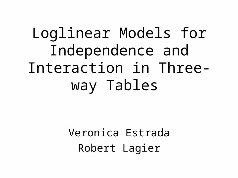
Quick Review from Agresti, 4.3

• Poisson Loglinear Models are based on Poisson distribution of Y counts and employ log link function:

log μY = α + βx

μY = exp(α + βx)

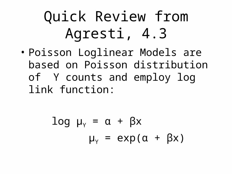
Value of Loglinear Models?

• Used to model cell counts in contingency tables where at least 2 variables are response variables

• Specify how expected cell counts depend on levels of categorical variables

• Allow for analysis of association and interaction patterns among variables

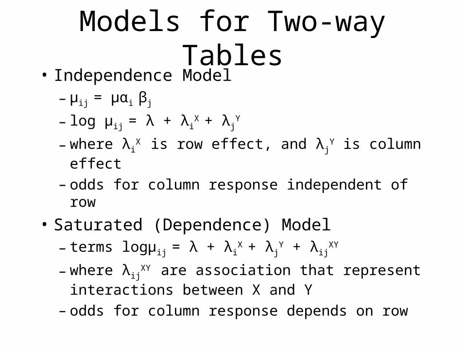
Models for Two-way Tables• Independence Model

– μij = μαi βj

– log μij = λ + λiX

+ λjY

– where λiX

is row effect, and λjY is column effect

– odds for column response independent of row

• Saturated (Dependence) Model– terms logμij = λ + λi

X + λj

Y + λijXY

– where λijXY

are association that represent interactions between X and Y

– odds for column response depends on row

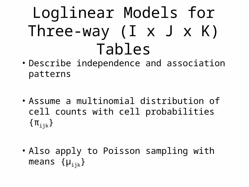
Loglinear Models for Three-way (I x J x K) Tables

• Describe independence and association patterns

• Assume a multinomial distribution of cell counts with cell probabilities {πijk}

• Also apply to Poisson sampling with means {µijk}

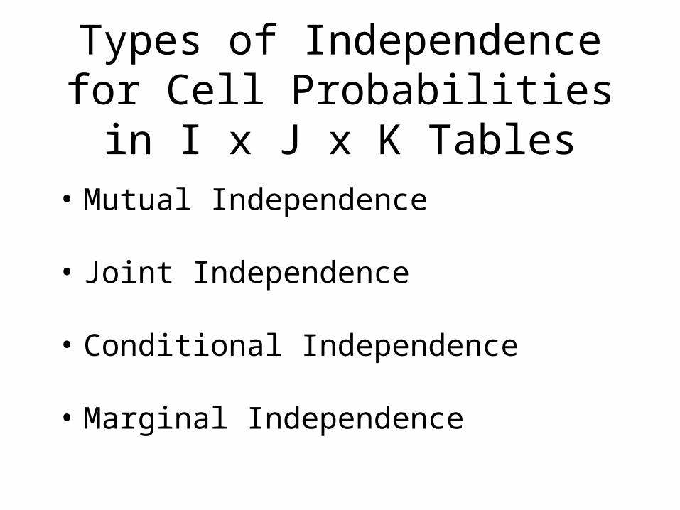
Types of Independence for Cell Probabilities in I x J x K Tables

• Mutual Independence

• Joint Independence

• Conditional Independence

• Marginal Independence

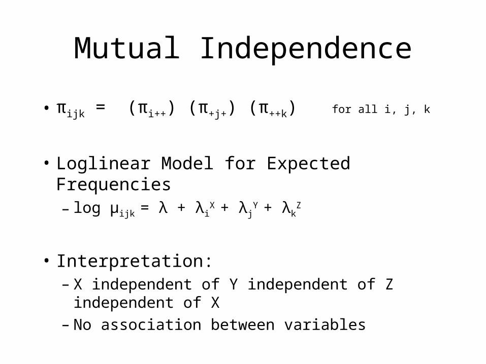
Mutual Independence

• πijk = (πi++) (π+j+) (π++k) for all i, j, k

• Loglinear Model for Expected Frequencies– log μijk = λ + λi

X + λj

Y + λkZ

• Interpretation:– X independent of Y independent of Z independent

of X– No association between variables

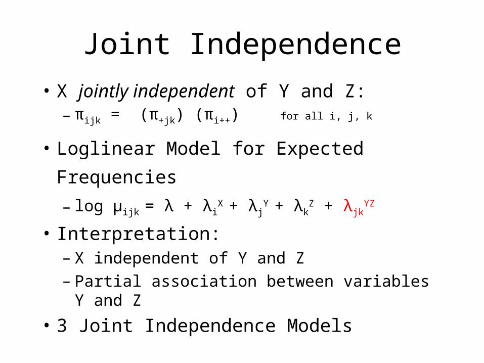
Joint Independence

• X jointly independent of Y and Z:– πijk = (π+jk) (πi++) for all i, j, k

• Loglinear Model for Expected Frequencies

– log μijk = λ + λiX

+ λjY + λk

Z + λjkYZ

• Interpretation:– X independent of Y and Z– Partial association between variables Y and Z

• 3 Joint Independence Models

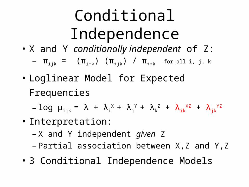
Conditional Independence

• X and Y conditionally independent of Z:– πijk = (πi+k) (π+jk) / π++k for all i, j, k

• Loglinear Model for Expected Frequencies

– log μijk = λ + λiX

+ λjY + λk

Z + λikXZ + λjk

YZ

• Interpretation:– X and Y independent given Z– Partial association between X,Z and Y,Z

• 3 Conditional Independence Models

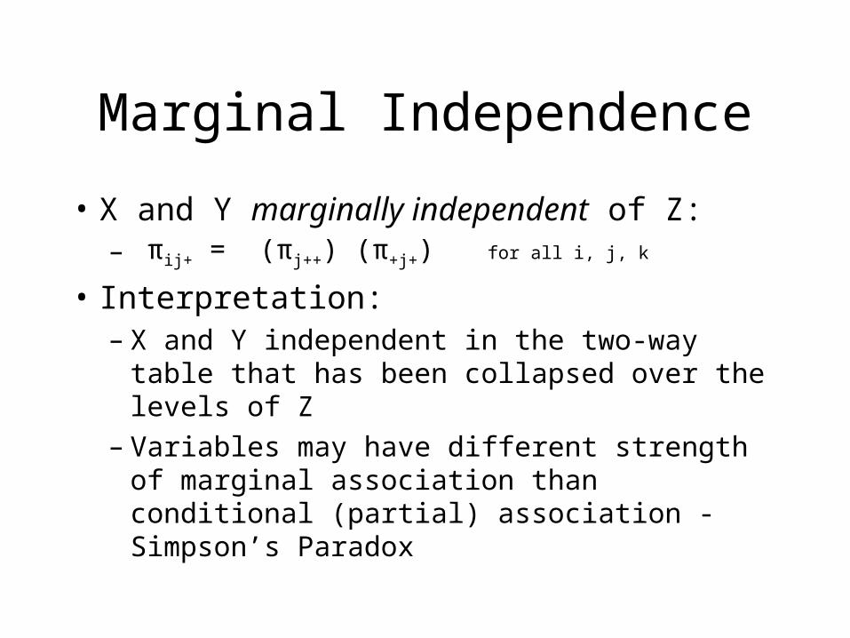
Marginal Independence

• X and Y marginally independent of Z:– πij+ = (πj++) (π+j+) for all i, j, k

• Interpretation:– X and Y independent in the two-way table that

has been collapsed over the levels of Z– Variables may have different strength of

marginal association than conditional (partial) association - Simpson’s Paradox

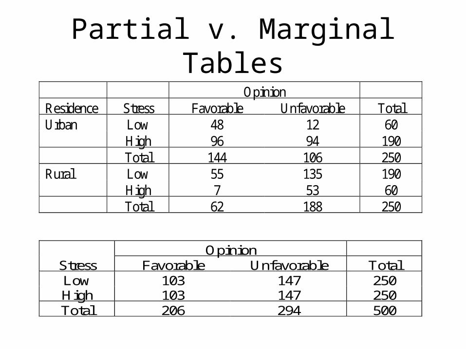
Partial v. Marginal TablesOpinion

Residence Stress Favorable Unfavorable TotalLow 48 12 60UrbanHigh 96 94 190Total 144 106 250Low 55 135 190RuralHigh 7 53 60Total 62 188 250

OpinionStress Favorable Unfavorable TotalLow 103 147 250High 103 147 250Total 206 294 500

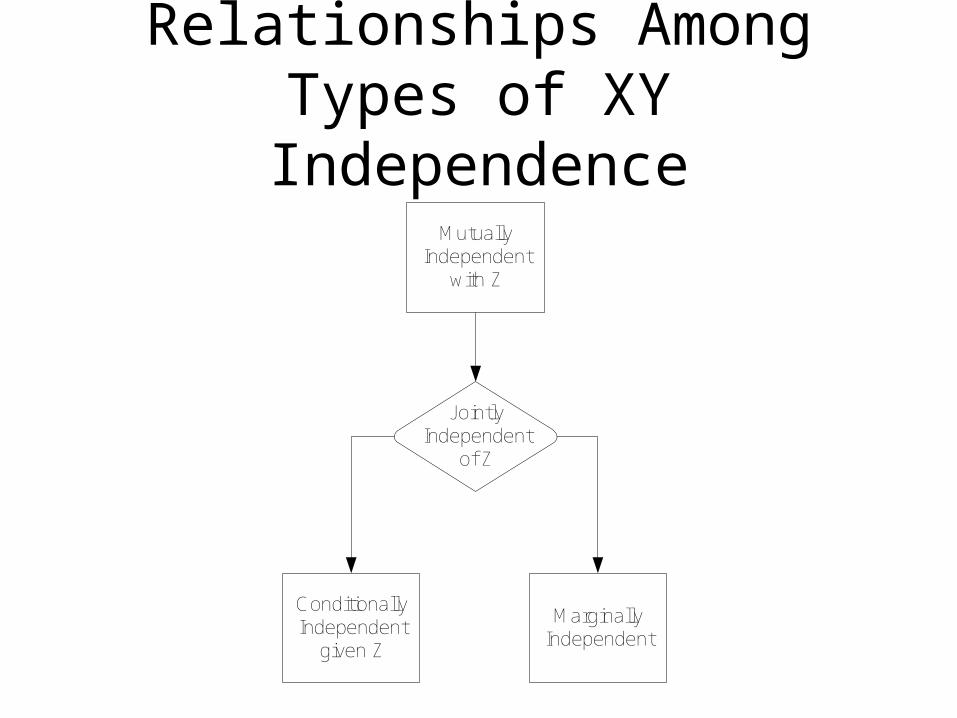
Relationships Among Types of XY Independence

MutuallyIndependent

with Z

ConditionallyIndependent

given Z

MarginallyIndependent

JointlyIndependent

of Z

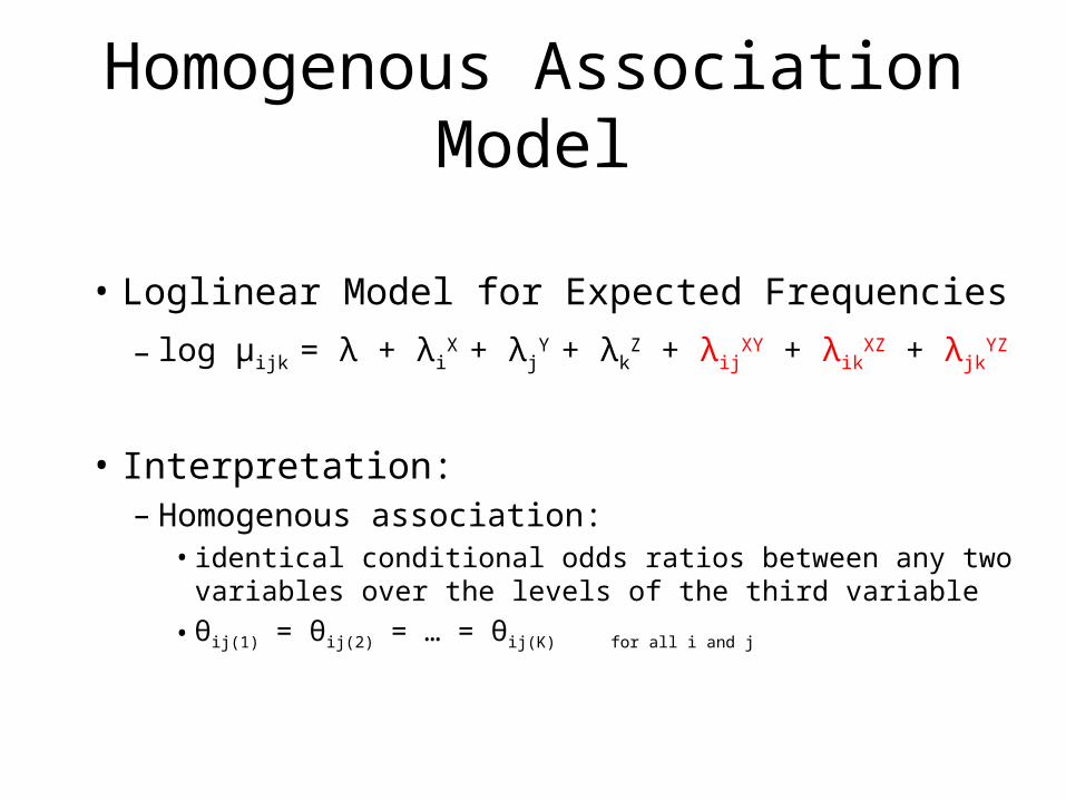
Homogenous Association Model

• Loglinear Model for Expected Frequencies

– log μijk = λ + λiX

+ λjY + λk

Z + λijXY + λik

XZ + λjkYZ

• Interpretation:– Homogenous association:

• identical conditional odds ratios between any two variables over the levels of the third variable

• θij(1) = θij(2) = … = θij(K) for all i and j

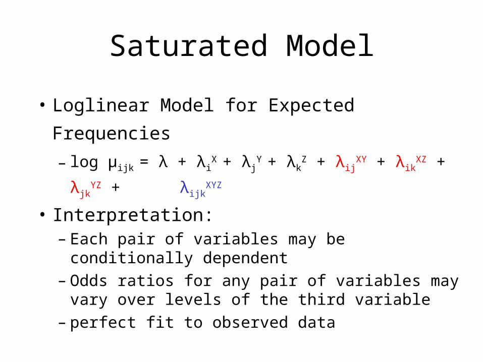
Saturated Model

• Loglinear Model for Expected Frequencies

– log μijk = λ + λiX

+ λjY + λk

Z + λijXY + λik

XZ + λjkYZ +

λijkXYZ

• Interpretation:– Each pair of variables may be conditionally

dependent– Odds ratios for any pair of variables may vary over

levels of the third variable– perfect fit to observed data

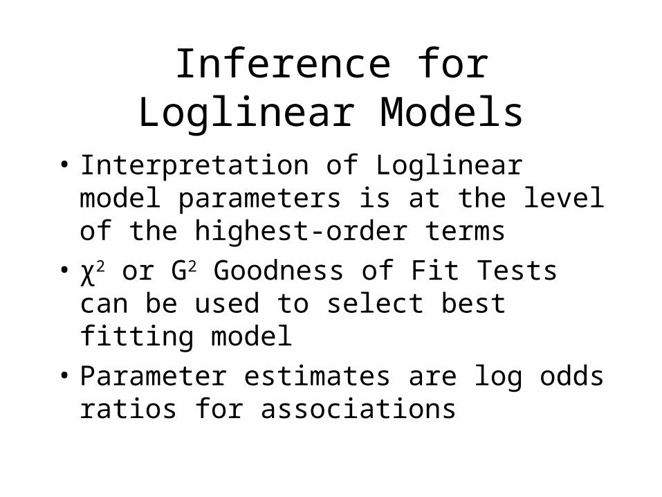
Inference for Loglinear Models

• Interpretation of Loglinear model parameters is at the level of the highest-order terms

• χ2 or G2 Goodness of Fit Tests can be used to select best fitting model

• Parameter estimates are log odds ratios for associations

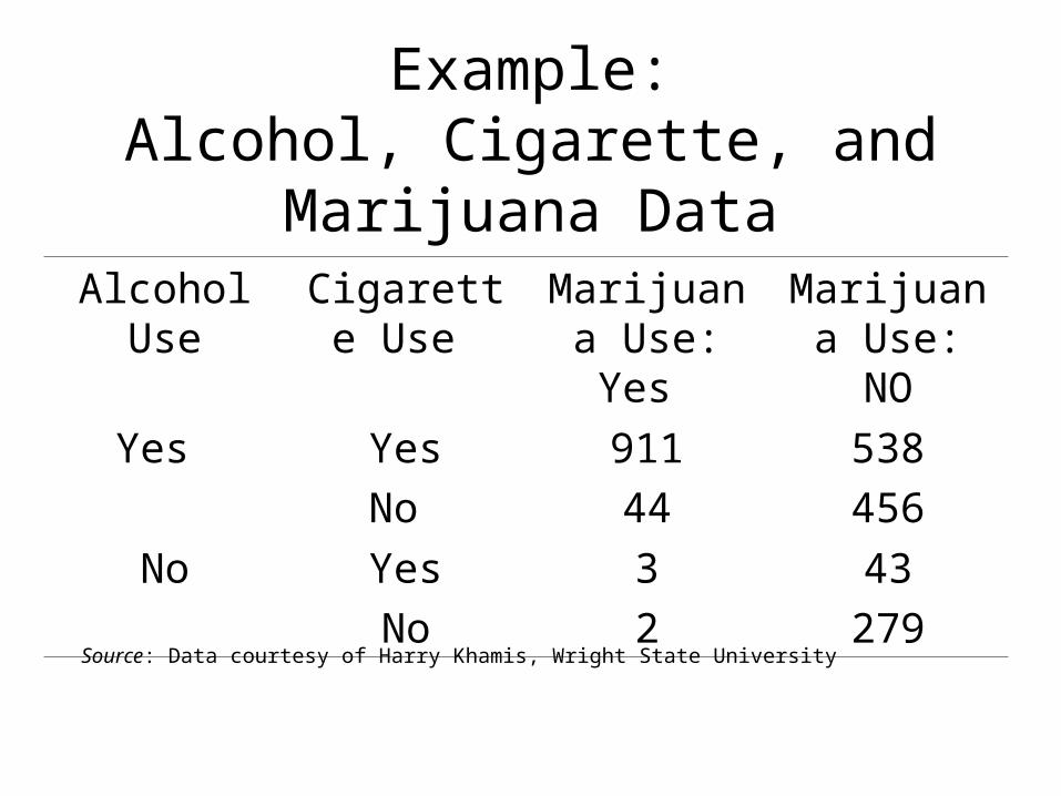
Example:Alcohol, Cigarette, and Marijuana

DataAlcohol Use Cigarette

Use Marijuana Use: Yes

Marijuana Use: NO

Yes Yes

No

911

44

538

456

No Yes

No

3

2

43

279

Source: Data courtesy of Harry Khamis, Wright State University

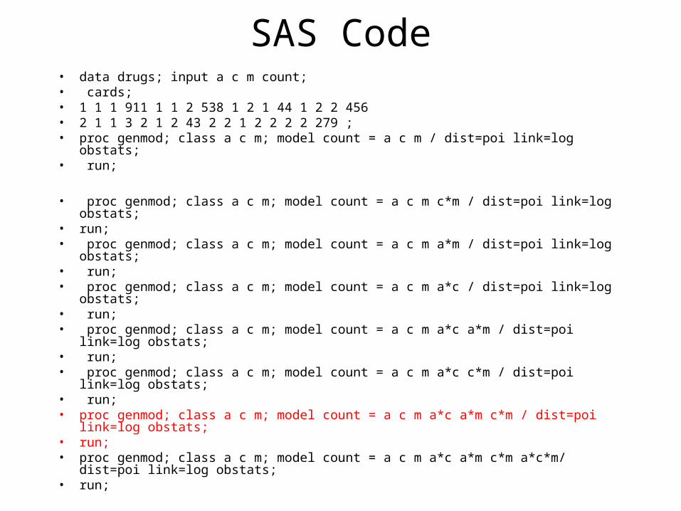
SAS Code• data drugs; input a c m count;• cards; • 1 1 1 911 1 1 2 538 1 2 1 44 1 2 2 456 • 2 1 1 3 2 1 2 43 2 2 1 2 2 2 2 279 ; • proc genmod; class a c m; model count = a c m / dist=poi link=log obstats;• run;

• proc genmod; class a c m; model count = a c m c*m / dist=poi link=log obstats; • run;• proc genmod; class a c m; model count = a c m a*m / dist=poi link=log obstats;• run;• proc genmod; class a c m; model count = a c m a*c / dist=poi link=log obstats;• run;• proc genmod; class a c m; model count = a c m a*c a*m / dist=poi link=log obstats;• run;• proc genmod; class a c m; model count = a c m a*c c*m / dist=poi link=log obstats;• run; • proc genmod; class a c m; model count = a c m a*c a*m c*m / dist=poi link=log obstats; • run; • proc genmod; class a c m; model count = a c m a*c a*m c*m a*c*m/ dist=poi link=log

obstats; • run;

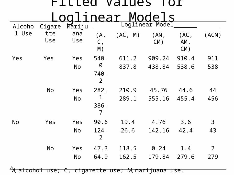
Fitted Values for Loglinear Models Alcohol

UseCigarette

UseMarijuan

a Use (A, C, M)

(AC, M) (AM, CM)

(AC, AM, CM)

(ACM)

Yes Yes Yes

No

540.0

740.2

611.2

837.8

909.24

438.84

910.4

538.6

911

538

No Yes

No

282.1

386.7

210.9

289.1

45.76

555.16

44.6

455.4

44

456

No Yes Yes

No

90.6

124.2

19.4

26.6

4.76

142.16

3.6

42.4

3

43

No Yes

No

47.3

64.9

118.5

162.5

0.24

179.84

1.4

279.6

2

279

Loglinear Model

A, alcohol use; C, cigarette use; M, marijuana use.a

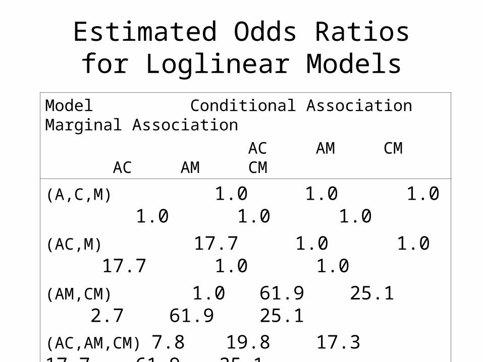
Estimated Odds Ratios for Loglinear Models

Model Conditional Association Marginal Association

AC AM CM AC AM CM

(A,C,M) 1.0 1.0 1.0 1.0 1.0 1.0

(AC,M) 17.7 1.0 1.0 17.7 1.0 1.0

(AM,CM) 1.0 61.9 25.1 2.7 61.9 25.1

(AC,AM,CM) 7.8 19.8 17.3 17.7 61.9 25.1

(ACM) 13.8 24.3 17.5 17.7 61.9 25.1

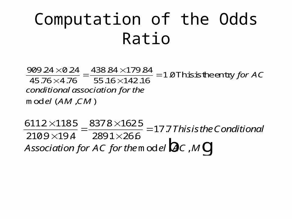
Computation of the Odds Ratio

6112 118 5

210 9 19 4

837 8 162 5

289 1 26 617 7

. .

. .

. .

. ..

mod ,

Thisis theConditional

Association for AC for the el AC Mb g

909.24 0.24

45.76 4.76

438.84 179.84

55.16 142.161.0Thisis theentry

for AC

conditional association for the

el AM CMmod ( , )

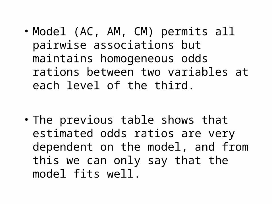
• Model (AC, AM, CM) permits all pairwise associations but maintains homogeneous odds rations between two variables at each level of the third.

• The previous table shows that estimated odds ratios are very dependent on the model, and from this we can only say that the model fits well.

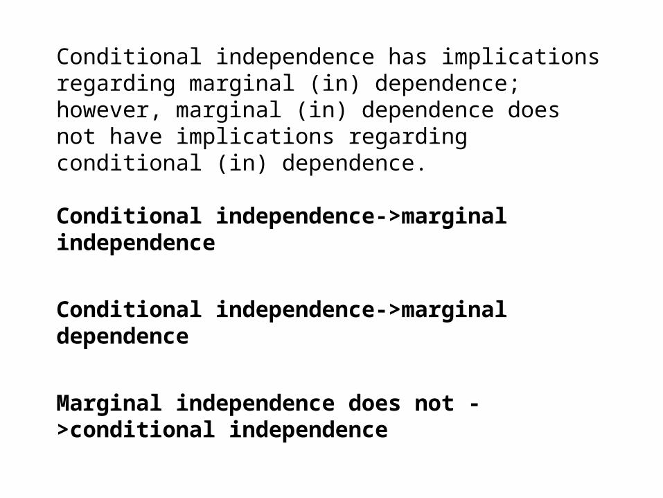
Conditional independence has implications regarding marginal (in) dependence; however, marginal (in) dependence does not have implications regarding conditional (in) dependence.

Conditional independence->marginal independence

Conditional independence->marginal dependence

Marginal independence does not ->conditional independence

Marginal dependence does not ->conditional dependence.