Loglinear multidimensional IRT models for polytomously

PSYCHOMETRIKA--VOL. 59, NO. 2, 149-176 JUNE 1994

LOGLINEAR MULTIDIMENSIONAL IRT MODELS FOR POLYTOMOUSLY SCORED ITEMS

HENK KELDERMAN AND CARL P. M. RIJKES 1

UNIVERSITY OF TWENTE

A loglinear IRT model is proposed that relates polytomously scored item responses to a multidimensional latent space. The analyst may specify a response function for each response, indicating which latent abilities are necessary to arrive at that response. Each item may have a different number of response categories, so that free response items are more easily analyzed. Conditional maximum likelihood estimates are derived and the models may be tested generally or against alternative loglinear IRT models.

Key words: multidimensional item response theory, loglinear model, Rasch model, multidimensional Rasch model, polytomous responses, partial credit model, goodness-of-fit testing.

Educational and psychological tests or item banks are ordinarily used to measure individual differences that are inferred from behavior. A test typically consist of a set of items varying with respect to certain task properties that may present difficulties the subject has to overcome to give the correct response. Most tests are constructed in such a way that each item presents a problem that can be solved by some characteristic cognitive behavior that the test intends to measure. Item properties that present problems irrelevant to the measurement purpose are manipulated in such a way that they become very easy for most subjects. In this way items are constructed that measure the behavior of interest.

Item response theory (IRT) models, such as the one-, two- and three-parameter logistic model are suited to explain a subject's response on each of the items by a subject parameter and one or more item parameters. Typically, model parameters characterize both items and subjects on one single latent trait. Likewise, for the case of polytomously scored items, IRT models have been proposed that relate responses to a single underlying latent trait (Andrich, 1978, 1982; Bock, 1972; Glas & Verhelst, 1989; Masters, 1982; Muraki, 1990; Rost, 1988; Samejima, 1972; Thissen & Steinberg, 1984).

In practice, the construct to be measured may be more complex than can be modeled by such IRT models. In test construction research it may be desirable to go further and specify theories that explain what the items are measuring. By specifying a model for each theory and comparing the fit of those models to the data, considerable knowledge about what the items measure can be gained (Stenner, Smith, & Burdick, 1983). These theories concentrate on the cognitive process rather than the products measured by the test (Sternberg, 1982, p. 1). For example, Frederiksen (1982) in his study of reading skills, specified several component behaviors, which in interaction with one another, accomplish the more complex performance of reading with compre- hension.

I Hank Kelderman is currently affiliated with Vrije Universiteit, Amsterdam. We thank Linda Vodegel-Matzen of the Division of Developmental Psychology of the University of

Amsterdam for making available the data used in the example in this article. Requests for reprints should be sent to H. Kelderman, Department of Work and Organizational Psychology, Faculty of Psychology and Pedagogics, Vrije Universiteit, De Boelelaan 1081c, NL 1081 HV Amsterdam, THE NETHERLANDS.

0033-3123/94/0600-92078500.75/0 © 1994 The Psychometric Society

149

150 PSYCHOMETRIKA

Variation in task properties of items can have two types of effects. It may have a quantitative effect on the problem that the item presents. That is, some items may become more difficult to answer correctly than others. At the same time, items may order subjects in terms of ability in the same way, because they require the same type of problem solving behavior. On the other hand, variation in item task properties may lead to problems that are qualitatively different requiring different types of problem solving behavior, so that subjects have a different ordering in achievement on different items. In this case, individual differences must be described by a multidimensional latent space.

A model that describes problems that differ quantitatively is the linear logistic test model (LLTM, Fischer, 1973; Fischer & Forman, 1982; Scheiblechner, 1972). LLTM models view an item as consisting of different subtasks, where each subtask presents a proble m with a certain difficulty. Usually only a limited number of subtasks are assumed of which each item requires a certain subset. In the LLTM it is assumed that the problems that the subtests present differ quantitatively but not qualitatively. Therefore, the models contain a single subject parameter, so that subjects have the same orderings in achievement on different items. Spada (1976) successfully applied LLTM models to relate performance on a test of the concept of proportions to the ability to perform certain cognitive operations.

Models for theories describing qualitatively different problems are Fischer's (1972, 1976) linear logistic test model with relaxed assumptions (LLRA) and Embretson's (1985) component latent trait models (CLTM). In LLRA, a different latent parameter is associated with each item. Each item is then administered at different points in time to measure changes in difficulty due to treatment effects. In CLTM, different cognitive components are associated with different latent trait parameters. In these models items may have a different specification of cognitive components; they may order subjects' achievements differently.

In attitude research, Duncan and Stenbeck (1987) analyzed Likert scales using a multitrait Rasch model. Two traits were distinguished: Content and power. The model generalizes the unidimensional Rasch rating scale model (Andrich, 1978, 1982; Masters, 1982). Duncan and Stenbeck's model is based on the analysis of contingency tables by loglinear models.

Loglinear models have been used for the estimation and testing of IRT models (Cressie & Holland, 1983; de Leeuw & Verhelst, 1986; Duncan, 1984; Kelderman, 1984; Tjur, 1982). They have proved useful in the solution of practical psychometric problems such as item bias detection and equating.

In the present paper, a loglinear IRT model is proposed that applies to the situation of polytomously scored test items that may be explained by a multidimensional latent space. The model generalizes Duncan and Stenbeck's (1987) model for Likert scales and Andersen's (1983) latent structure model for contingency table data. The flexibility and generality of loglinear IRT modeling enables the researcher to formulate a model precisely tailored to the particular items in the test. In the proposed model, each response may involve several cognitive operations defined by the user, and different cognitive operations may require different abilities. Each item may have a different number of response categories, so that free response items are more easily analyzed. The usual assumption of local independence of the item responses given the latent traits is made. The item parameters are estimated by the conditional maximum likelihood method and the goodness-of-fit of the models can be tested either overall or against specific deviations from the model.


A Multidimensional Polytomous Latent Trait Model

Suppose that each of N subjects respond to k test items where the answers of subject i to i t emj may be any of rj + 1 responses xij ( x i j = O, . . . , r j ) . I f its meaning is unambiguous, rj will be denoted as r. The response pattern of subject i on all k test items is denoted by the vector x i = ( X n , xi2, • • • , x ik ) . The corresponding random variables or vectors are denoted by capital letters Xi j and Xi.

Let Oiq be a value of subject i on a latent trait q = 1 . . . . , s, and let 0i = (Oil , 0i2 . . . . . Ois) be the subject 's vector of latent trait values. To produce a score xi j on item j , subject i must perform certain cognitive operations where each operat ion depends on a certain proficiency on a latent trait. For example, to produce a correct answer on the item "Wha t is the square root of fifteen minus s ix?" , involves three operations. First, the expression V/(15 - 6) must be obtained from the verbal formulation. Second, the subject must make the subtraction 15 - 6 = 9. And finally, the square root V ~ = -+3 must be taken. It may be hypothesized that to perform the first operation successfully, the subject must have a certain level on a verbal ability trait Oil, and to perform the second and the third operation, a latent numerical ability 0i2 is needed. Because the correct response depends more heavily on the second latent trait than on the first, it may be expected that 0i2 has a stronger impact on individual differences in the response than 0il .

Let Bjqx be a nonnegative weight associated with the dependence of a generic response x to i t emj on the latent trait q (= 1 . . . . . s). In the next section it is seen that Bjq x enters the sufficient statistics of the subject parameters. It is, therefore, called the scoring weight. Fur thermore, let 6jq x be a parameter describing the difficulty of response x to i t emj related to latent trait q, and let ~ j = ( 6 j l 0 . . . . , 6 j l r , 6 j20 , " ' " , 6jsr) be the vector of difficulty parameters for item j . The multidimensional polytomous latent trait model (MPLT) can now be written as

exp[ ..x.x] e(xij xlOi) q = 1 = = , ( 1 )

c(Oi, ~j)

with constant of proportionali ty

C(Oi, ~) = E exp y=0

lq~ l (Oiq- ~jqy)Bjqy].

Here, it is assumed that 6jqx = 0 if njq x = 0 to ensure uniqueness of the parameter . By choosing the scoring weights Bjqx appropriately (x = 0, . . . , rj; j = 1, . . . , k; q = 1 . . . . . s), different models can be defined for the dependence of item responses on latent traits. If a weight is zero, the subject 's position on the latent trait does not influence the probability of the particular response. If a scoring weight is large, the response is heavily influenced by the trait. For technical reasons to be discussed later, it is assumed that weights take discrete values (0, I, 2 . . . . ). For the traits whose weights are not zero, a larger positive difference between the subject parameter Oiq and the difficulty parameter 6jqx yields a larger probability of the particular response. Model (1) is a Rasch type model. As we shall see later, it generalizes many Rasch models such as the dichotomous Rasch model and the Partial Credit model. An advantage of its exponential form is the separability of the person and item parameters.

152 PSYCHOMETRIKA

If the items are dichotomously scored, the MPLT model may be compared to Fischer's (1973) LLTM, which also has an exponential form

e x x 0 i - r l q Q j q

= 1 e ( x i j = x l O i ) =

1 + exp Oi - " r l q Q j q

= 1

where Oi is a single subject parameter, ~Tq (q = 1, . . . , s) are component difficulty parameters and Qjq ( j = 1 . . . . , k; q = 1, . . . , s) are weights. The difference with the MPLT model is that in the LLTM, the weights Qjq are only applied to the component difficulty parameters and not to the subject parameters. Furthermore, in LLTM it is assumed that the component subtasks q do not require a different latent subject parameter, whereas in the MPLT model, each component involves a parameter for both the item (response) and the subject.

Fischer's LLRA is like the MPLT model (1) in that it may specify a multidimensional latent space. LLRA relaxes the LLTM model such that different subject parameters are postulated for each of the items, where each item is administered repeatedly. Embretson's (1984, 1985) general latent trait model (GLTM) may contain more than one latent trait. The model includes a product of LLTM models, one for each latent trait, and a guessing parameter. An important difference between the MPLT model and the GLTM is that the former is an exponential family model, and that sufficient statistics for the parameters exist.

Model (1) is completely general in that each item may have a different number of answer categories, and for each item response, the user may specify a scoring weight. This flexibility allows the specification of models that closely follow theoretical ideas that explain what the items are measuring. We now consider some submodels of (1). Figure 1 gives some examples of scoring weights that might be employed, and which will be used as illustrations in the section to follow. In Figure 1, several choices ofBjq x are given for combinations of x and q. Note that these diagrams each specify the scoring weights only for one i temj and that many more specifications of scoring weights are possible.

Some Examples of MPLT Models

To illustrate the type of models that can be formulated within the general framework of MPLT models, this section discusses five submodels and some variants. Three models are well-known: The Rasch model for dichotomously scored items, the partial credit models, and Rasch's multidimensional models. These examples show how the MPLT is related to some known IRT models and how the parameters of these models can be calculated from the parameters of the MPLT model. Two other models are new: A model for items with two correct responses and a multidimensional version of the partial credit model (see Wilson, 1989, 1990, for other examples of MPLT models).

The D i c h o t o m o u s R a s c h M o d e l

Figure la describes the scoring weights for an item following the dichotomous Rasch model (Rasch, 1980). A wrong response (x = 0) is scored Bjlo = 0 and a correct response (x = 1) is scored Bi l l = 1. Substituting these scoring weights in (1) and omitting the latent trait index q, yields the model


0

1

q

1

[a]

q

1

0 0

1 1

2

[b]

0

x 1

2

q

1

0

[c]

X 0

1

q

1

[d]

q

1 2

0 0 0

x 1 1 0

2 0 1

[e]

X

0

1

2

q

1 2

0 0

1 0

0 2

[f]

X

q

1 2

0 0 0

1 1 0

2 1 1

[g]

X

1

0 0

1 1

[h]

q

2

0

FiouP~ 1. Examples of scoring weights.

q

1 2

0 0 0

1 1 0 X

2 2 0

3 2 1

[il

154 PSYCHOMETRIKA

so that

exp [ (0 i -- 6 j x ) X ]

P ( x i j = xlOi) exp [OiO -- 6j00 ] + exp [ O i l - 6 j l 1] ' (2)

exp [Oi - 6jl] e ( x i j = l lOi)=

I + exp [O i - t~jl ]"

In (2), 6j0 = 0 since B jl o = 0; otherwise, the model would be indeterminate. Also, one additional linear constraint, say 611 = 0, must be imposed in the response parameters to fix the scale.

A Model with Two Correct or Incorrect Responses

Figure lb describes the scoring weights for an item with three possible responses: 0, 1, and 2. The responses x = 1 and x = 2 both correspond to a correct answer. For example, the question: "Wha t is the value o f x in x 2 + 2 = 6 ? " , may be answered +2 or - 2 . In the model of Figure lb it is assumed that both correct responses pertain to the same latent trait, but one answer may be more likely than the other since the parameters 6jl and 6j2 may differ. For items with several distinguishable incorrect responses, similar scoring weights may be formulated.

The Partial Credit Model

Figure lc also describes an item with three responses, but here each response has a different weight. The response x = 2 has the weight 2, x = 1 has weight 1, implying that response 2 has a stronger relation to the latent trait than response 1. As before the wrong response x = 0 has weight 0 and 6jo = 0. With these scoring weights and omitting the latent trait index q, (1) becomes

exp [(Oi - 6ix)X]

rj

Z y=0

P(Xij : x]Oi) =

1 +

exp [(0 i - - 6jy)y]

Xp[g ,0 1 ~'~ exp (Oi - Ojg)

y = l g = l

where

(3)

x x - - l

~bjx = ~ ~bjg- ~ ~bjg = X S j x - ( X - 1)r j (x-1) , g = l g = l

which is the polytomous Rasch model for ordered categories, or the partial credit model (Andrich, 1978; Masters, 1982; Wright & Masters, 1982). To distinguish this model from a multidimensional Rasch model treated later, the model will be referred to as the unidimensional partial credit model (UPCM).

The partial credit model suggests a useful interpretation of the scoring weights.


Each response may be seen as the result of a series of subsequent steps, each of which has to be passed. To arrive at response x, x steps must be performed. Denote a step by 9. In step 9 (= 1 . . . . , x), there is a cognitive process that requires latent trait Oi. In (3), each step enters as a term (Oi - qJjg), where the parameter Sjg describes the difficulty of step 9 in item j . The step probability of giving response x rather than x - I follows a simple dichotomous Rasch model (2)

P(Xi j = xlXij = x or x - 1, Oi) = P(Xi j = xlOi)

P(Xi j = xlOi) + P(Xi j = x - l lOi)

exp [Oi - $ i x ]

1 + exp [Oi - ~ j x ] '

with subject parameter 0 / a n d response difficulty parameter ~jx2 ,, As an example of a partial credit model, consider the item ( X / ~ - 6) = ? . The

partial response "X/9" is scored x = 1. This is the result of the first step in the solution process. To arrive at this partially correct response, the latent trait Oi has to be applied once. Fur thermore, the completely correct response ``+ 3" is scored x = 2. To produce response "---3", ability Oi has to be a a_pplied twice, once to do the first step 15 - 6 = 9, and once to do the second step V 9 = +3. The steps concept leads to the scoring weights Bjlx = x (x = 0, 1, . . . ), defined as the number of steps (involving trait 1) needed to arrive at the response starting from category zero. In this example it is assumed that there is one arithmetic latent trait. In the next example, we will consider a model that postulates two latent traits.

The steps concept may also be adopted in the general context of (1) where Bjqx is the number of steps or cognitive processes (involving trait q) necessary to arrive at response x starting from zero. Note that, in general, the results of these steps are not necessarily observed as responses. For example, if the partial response " 9 " is not observed, there are two responses, incorrect (x = 0) and correct "---3" (scored, say, x = 1). The correct response " - 3 " , however, may still be viewed as the result of two steps, "15 - 6 = 9" and "X/'9 = 3" . This leads to the scoring weight Bi l l = 2, as depicted in Figure 1 d.

Rasch Mult idimensional Model

In Figure le the responses x = 1 and x = 2 each depend on a different latent trait, both with scoring weights equal to one. Thus, with q = I , 2, and x = 0, 1, 2, we have Bjq x = 1 if q = x, and Bjq x = 0, otherwise. Substituting these scoring weights in (1) yields

exp [ 0 ix - 6jxx ] P(Xl j = xlOi) = , (4)

rj

1 + ~ exp [Oig - 8jgg] g = l

for x = 1, 2, and

e ( x u = olo~) = rl

I + ~ e x p [ 0 i g - ~ j g g ] g = l

156 PSYCHOMETRIKA

for x = 0. This is the multidimensional Rasch model described by Rasch (1961) and Andersen (1973), where each category x = I, . . . , rj depends on a different latent trait. Andersen applied the model to multiple choice items on job satisfaction. In the cognitive domain, the model may be applied to free response items where different responses pertain to different solution strategies.

For example, the question "Wha t are the roots of the equation x 2 + x - 2 = 0 ? " may be solved by substitution of a = 1, b = 1, and c = - 2 in the learned formula [ - b +-- V ' (b z - 4ac)]/2a, or it may be solved by rewriting it as (x - 1)(x - 2) = 0, and choosing x so that a factor becomes zero. I f a response indicates that the first strategy is used (x = I) , it is hypothesized that the response required latent trait Oil ; if the response indicates that the second strategy is used (x = 2); latent trait 0i2 is assumed. Andersen (1983) also describes a generalization of the multidimensional Ra- sch model, depicted in Figure If, where each response depends on its own latent trait but the item weights are not all equal to one.

A Mult idimensional Partial Credit Mode l

Figure Ig describes a multidimensional partial credit model (MPCM) where each step depends on a different latent trait. The correct response x = 2 has scoring weight BjI 2 = 1 on the first trait and scoring weight B j2 ~ = 1 on the second. The partially correct response x = 1 has scoring weight By11 = 1 on the first latent trait, and the incorrect response x = 0 has weight zero. Substituting these scoring weights in (1) yields

P(Xij = x l 0 1 ) = q = 1

I 1" 1 +___~ exp (0 iq - ~Joy) y = l q = l

However , there is an indeterminacy between the difi~culty parameters 8jqx of different responses x within the same latent trait q and item j . Because the response difficulty parameters for response x enter the model through Zq=lx 8jqx, only, adding a constant c t o ~jqy and subtracting it f rom 8jqy, (1 ~- y ' <- x , I <- y ~- x , y ' # y ) , does not change the model. This indeterminacy can be removed by setting the response difficulty parameters of the same response x equal to each other; that is Ojq = ~jqx for x = 1 . . . . , r j , giving

exp ~ (Oio - Ojq)

P ( X o = xl0D = q ~ 1 .................... (5)

1 +_..~ e x p (Oiq - i~tjq) y = , t q - - I

In the MPCM (5), like in the UPCM (3), each response may be seen as the result o f a series of subsequent steps. To arrive at response x, x steps q (= 1 . . . . . x) must be performed. In the MPCM, each step depends on a different latent trait Oiq. From (5) it is readily shown that, as in the one-dimensional partial credit model, the step probability P(Xi j = xIXij = x or x - 1, 0i) of giving response x rather that x - 1 follows


a simple dichotomous Rasch model (2) with subject parameters Oiq and response difficulty parameter d/jq.

The MPCM might be an alternative model for the item "%/(15 - 6) = ?". The first step "15 - 6 = 9" requires "subtraction" depending on the latent trait 0il and the second step "V:9 = ±3" requires "taking the square root" depending on 0i2. The partial response 9 (or vr9) pertains to Oil and the complete response -+3 pertains to both 0il and 0i2.

Figure lh is a two-dimensional model for a dichotomous item. This model can be obtained from the MPCM in Figure lg by omitting the partial response and relabeling the complete response as x = 1. The model is a two-dimensional Rasch model. Just as in the MPCM, the latent traits may be related to subsequent steps in the solution process. Obviously, a combination of UPCM and MPCM, where there are different latent traits but some operations depend on the same latent trait, is also possible. Figure li, for example, may model the item %/(20 - 5 - 6), where there are two subtractions and one square root.

We have discussed some examples for scoring weights. There may be many other choices for scoring weights than shown here that make sense in a particular application, and moreover, different items may have different patterns of scoring weights. For example, one item may follow the dichotomous Rasch model, and another item the partial credit model, and so on.

Estimation and Testing

In this section conditional maximum likelihood estimates of the response parameters are derived. The model is formulated for the joint responses of k items. By conditioning on sufficient statistics for the subject parameters, a quasi-loglinear model arises that contains item response parameters only. The maximum likelihood equations for this model can be solved by standard methods, and can be tested by overall goodness-of-fit tests or compared with alternative loglinear models.

To simplify subsequent equations, write the weighted sums over latent traits of the item response parameters as a single parameter,

so that (1) becomes

where

$

dPjx = -- Z 8 jqxBjqx ' q = l

P ( X U = x l O i ) =

exp [ q ~ = l Oiqnjqx + ¢~jx] C(01, • j )

, ( 6 )

c(a/, ,l,j)-- r ]

e x p OiqBjqy + ~bjy , y=0 q = l

is the proportionality constant. Note that if we allow ¢kjx in (6) to be nonzero when the B j l x , . . . , B j s x are all equal to zero, the model becomes slightly more general than (1).

158 PSYCHOMETRIKA

This relaxation allows a variable that is unrelated to all latent traits to have different probabilities for each of its response categories. In this case, (6) becomes

exp [4~jx] P(Xij = x) = (7)

rj

~'~ exp [q~Jr] y = O

This relaxation is useful to add one or more background variables (e.g., sex or age) to the model.

Denote the joint observed random response variables by x i = (X i l , . . . , X ik) , which can take values xi = (xil . . . . . Xik). Assume that the Xij are conditionally (or locally) independent of each other given the latent traits 0i = (0il , . . . , Ois):

k

e ( x i = xilO~) : I1 e(xij : xii loi) . (8) j = l

Let &j = (~bjo . . . . . C~jr) be the vector of response parameters of item j , t i q = ~'?=1 Bi~x is subject i 's sum of scoring weights for latent trait q, and T i a is the corresponding random variable. Substitution of (6) in (8) gives the joint distributio of Xi g" en 0i,

P ( X i = xilO/) = exp Oiqtiq + ~ 4~j~o I-[ [c(Oi, 4~i)-1]. (9) 1 j = l j = l

Model (9) is an exponential family model and t i = ( t i l , . . . , t i s ) is a sufficient statistic for 0i = (Oil . . . . . Ois). Intuitively, we can see that the Oiq influence the probability of Xi = xi only through the sums of weights t i q ( q = l , • • • , s ) . Note that in the dichotomous Rasch model (Bjlx = x, x = 0, 1), t i l is equal to the number of correct responses. More formally, sufficiency of t i for Oi implies that the conditional distribution of Xi given t i is independent of 0i for all t i (Lehmann, 1983, p. 36). To show this, we derive the simultaneous distribution of the weight sum variables T i =

( T / t , . . . , T i s ) and divide it into the distribution of Xi. Let Y~x, ltt denote summation over all possible values of the item response vector xi

for which the weight sum vector equals t i. Applying this sum operator to the joint distribution (9) of Xi given 0i, yields the distribution of T i given 0i:

P ( T i = t i lOz)= ~ P(Xi = xilO~)= y( t / , * ) exp Oiqtiq H c(Oi, ~j)--l, xilt~ 1 j = 1

( lo)

where

with ~ = ($10, - • " , 4~1r,, - - - , 4'k0, - . - , 4'kr) is a generalization of the well-known elementary symmetric function.

The conditional distribution of X i given t i and 0/ is obtained by dividing the distribution (9) of Xi given 0i by the distribution (10) of T i given 0i:


P ( X i = xil0i) e ( x i = xi l t / , 0i) ---

P ( T i = til01)

ex,[ t T(ti , ~b)

= P ( X i = x / I t / ) , ( I I )

which no longer depends on 0 i. On the basis of (I 1), c o n d i t i o n a l m a x i m u m l i k e l i h o o d

e s t i m a t e s can be obtained for the item response parameters ¢b. Using (1 I) rather than (9), there is no need to estimate the latent trait parameters 0i for each subject i, nor do we need to assume a particular distribution for the latent traits. It is well-known that estimating both the ¢b and 0i parameters in (9), produces inconsistent estimates because the number of subject parameters 0i goes to infinity as the number of subjects goes to infinity (Neyman & Scott, 1948). So by conditioning out 0 i, this problem is neatly avoided.

Model (11) can be reformulated as a quasi-loglinear model for the f requency of a generic response pattern x given each weight sum pattern t, where the subject index i is dropped. Le t N t be the number of subjects with weight sum pattern t, and P(X = xlt) be identical to (1 I) without the subject index. The conditional expected frequency of the response pattern x given score vector t is then

mxt = N t e ( x = xlt), (12)

x = (x 1 . . . . , x k ) ; x 1 = 0 . . . . . r l ; . . . ; x k = O, . . . , r k ; t = ( t l , . . . , t s ) ; t l = Y . f=l B j l x j ; . . . ; t s = Y f = l B j s x j . Taking logarithms, we have the loglinear model,

k

log mxt = oft + ~'~ q~jxj. (13) j = l

Here, cr t = log (Nt/~,(t, 4)) is a proportionality constant and 4~jxj(J = 1, . . . , k; xj = O, . . . , r j ) are item response parameters to be estimated.

Model (13) is a quasi-loglinear model for an incomplete (Item 1 × Item 2 × • • • × I tem k × weight sum 1 × • • • × weight sum s) contingency table with expected counts mxt if tq = B l q x ~ + • • • + B k q x k , (q = 1, . . . , s), and structurally zero counts for tq # B l q x l + • • • + Bkqxk , ( q = 1, • • • , S) . Because of this incompleteness, the model is called quasi-loglinear rather than loglinear (Bishop, Fienberg, & Holland, 1975; sec. 5.4; Haberman, 1979, sec. 7.3).

Unless further restrictions are placed on the d~ parameters, they will not be iden- tifiable in general (see, for example, our discussion of the MPCM). To formulate identifiability conditions for (13), let log be an element-wise operator , mt is the vector of expected counts of all response patterns x with sums of weights t, d~ = ($10, • • • , ~bkr)', 1 = (1 . . . . , I)' is a vector of ones and D t is the design matrix with zero ' s and ones in the appropriate places. Then, (13) can be rewrit ten as

log mt = o' t l + Dtgb, (14)

The identifiability criteria are then (Imrey, Koch, & Stokes, 1981):

rank [1 Dt] = 1 + rank [Dt], (15)

160 PSYCHOMETRIKA

and

rank [D] = a, (16)

where D' = [D~, . . . , D~m~], and a is the number of columns of D (i.e., the number of parameters). Condition (16) ensures that the tk parameters are not linearly dependent upon each other, and condition (15) ensures they are not linearly dependent on the proportionality constants o" t.

If D does not satisfy these identifiability conditions, linear restrictions must be imposed on the parameters. Parameters that are linearly dependent on other parameters may be set to zero, which is equivalent to removing certain columns of D. Sometimes other identifying restrictions, such as setting sums of parameters to zero, enhance the interpretability of the parameters. An example of this will be given later. In deriving the likelihood equations, it is assumed that the identifiability conditions are met.

Let fxt be the observed number of subjects with (x, t), and l e t f xj be the marginal observed frequency of response xj on itemj. If it is assumed that the subjects respond independently of one another and t is considered fixed, the item response patterns have a product-multinomial distribution. Then, the observed data have the log likelihood

t xit

= t'~ x~lt fxt (j ~=1 ~bjxj+trt) +cOnstant k

= ~_~ 4~jxjf~ ~ + ~ Nttrt + constant. (17) j=l t

Here, the second equation is obtained by substitution of (13). Let mxX/be the marginal expected frequency of response xj and let Nt and m T be the observed and expected frequencies of weight sum t. Model (11) is an exponential family model with sufficient statistics fx~. Maximum likelihood equations can be obtained by taking the derivatives of the log hkehhood (17) for ~b and settmg them to zero (Haberman, 1979):

mxi , x j = O , . . . , rj; j = 1 . . . . , k,

Nt = mt T, for all t. (18)

Solving (18) for the parameters ~bjx yields maximum likelihood estimates. The solution can be obtained by iterative methods, such as iterative proportional fitting (IPF) or Newton-Raphson, that are standard in the analysis of incomplete contingency tables by loglinear models. See Bishop, Fienberg, and Holland (1975, chap. 5) or Haberman (1979, chap. 10) for a more complete account. Kelderman (1992) describes an algorithm especially constructed for the analysis of loglinear IRT models, which is implemented in the LOGIMO (Loglinear IRT Modeling) program (Ke!derman & Steen, 1988). LOGIMO is a Pascal program running on a VAX/VMS ol a 386 or higher PC/MS-DOS system. It can be obtained from iec P r o G A M M A , Box 841, 9700 AV Groningen, The Netherlands (E-mail: [email protected]).

Methods for exact overall goodness-of-fit tests for loglinear models are described by Baglivo, Olivier and Pagano (1992) but they cannot be used when there are more


than a few variables. Therefore we are limited to asymptotic overall goodness-of-fit statistics such as Pearson's goodness-of-fit statistic (X 2) and the likelihood-ratio statistic (G z). These statistics are asymptotically distributed as chi-square with degrees of freedom equal to the difference between the number of cells that are not structurally zero and the number of independent model parameters. If, however, the expected counts become too small, the approximation of the distribution of the overall likelihood-ratio statistic and the Pearson statistic by a chi-square distribution becomes poor (Koehler, 1977, 1986; Lancaster, 1961). Koehler (I986) shows however that if the number of cells and the number of subjects both become large and the expected counts are bounded below by some positive constant, the chi-squared approximation of the Pearson statistic is satisfactory, especially for tables in which the expected frequencies are not too different. If the expected frequencies are widely different however, the Pearson goodness-of-fit statistic will be too conservative and the likelihood-ratio statistic too liberal (Koehler, 1986, Table 3) and neither should be used to assess the fit of the model. See also Read and Cressie (1988) for a discussion of various overall goodness-of-fit statistics for discrete multivariate data. If such overall goodness-of-fit statistics cannot be used because of small cell counts, we can use statistics that are computed from contingency tables where cell counts are added together. By grouping cells together the chi-squared approximation of the statistic will generally improve.

The cells of the contingency table may be grouped into an item response × weight sum (marginal) contingency table. Such statistics are especially sensitive to misspeci- fication of the items' B-weights, the most important aspect of the model. For each of these grouped contingency tables the corresponding X 2 statistic is again distributed as chi-square with degrees of freedom equal to the number of independent cell counts. We will reject a B-weight specification if the right tail probability of the test statistic ex- ceeds the conventional .05 level. If misspecifications with these statistics are detected, residual plots may then be studied to generate ideas on how B-weights may be changed to improve model fit. The statistics based on the item response x weight sum table can be seen as generalizations of the van den Wollenberg (1982) Q1 statistics for testing the dichotomous Rasch model.

If several alternative models are available, it is useful to first compare the fit of these models before looking at their absolute fit. For this purpose statistics based on the likelihood ratio are more appropriate.

The likelihood ratio test statistic can be used if one model, say M, is a special case of another model, say M*. Let m* denote the expected counts under the larger model. The likelihood-ratio test statistic comparing both models is then

G2(m, m*) -2 (Lc * = - L c ) , (19)

which is asymptotically distributed as chi-square with degrees of freedom equal to the difference in numbers of linearly independent parameters of both models (Rao, 1973, pp. 418--420). Haberman (1977) showed that for large sparse contingency tables the chi-squared approximation of the likelihood-ratio statistic is appropriate when the difference in the degrees of freedom for the two models is much smaller than the total number of observations. This will usually be the case when comparing MPLT models. A drawback of this statistic is however that the two models must be nested, which is often not the case when comparing MPLT models.

Akaike's (1977) information criterion is useful when two models are not nested. The statistic in that case is

AIC = G 2 + 2 (# of parameters) + C,

162 PSYCHOMETRIKA

where C is a constant that is the same for all models fitted to the same data. The model with the smallest AIC (or AIC-C) is chosen as the best fitting. This procedure can be used to compare the fit of different MPLT models, as illustrated in the second example.

Examples

In this section MPLT models are applied to two sets of data. The first is a set of simulated data generated under a MPLT model, which gives an opportunity to compare the estimated parameters with their true values and the observed goodness-of-fit statistics with their expected values. The second example is a set of empirical test data that allows the testing of different hypotheses about the underlying latent structure. Both examples illustrate the analysis of data where different item responses have different latent trait specifications.

A n a l y s i s o f S i m u l a t e d D a t a

For the simulated data, there are eight items (one item with four possible responses and seven dichotomous items). Item 1 follows a three dimensional partial credit model; the dichotomous Item 2 also depends on all three latent traits. The remaining Items, 3 through 8, each follow a dichotomous Rasch model, where each latent trait is related to two of these items. Table 1 gives the model equations for this model (A).

Response patterns x i l , • • • , xi8 (i = 1, . . . , 14,000) were each generated in the following way. First, three latent trait values were drawn from a multivariate normal distribution N(O, X) with

X =

1.00 0.05 0.20

0.05 0.82 0.05

0.20 0.05 0.68

These numbers are chosen to have some variation in variances and covariances. Sec- ondly, item responses are generated according to the model equations in Table I with the true 8 parameters in Table 2. The item response parameters and latent trait variances were chosen so there was some variation in their values, but not producing extreme response probabilities (that is, between .20 and .80) for most of the subjects.

The data are analyzed with three models: A, B and C. Model A is the model under which the data are generated; Model B is a two-dimensional model that arises if the first two latent traits are assumed to be identical, and its model equations can be obtained from Table I by setting Oil and 0i2 equal to each other; Finally, Model C assumes that there is only one latent trait, and arises if all three latent traits are assumed equal. All three models correspond to a loglinear model (13) with different scoring weights.

Table 3 shows the goodness-of-fit statistics for Model A, B, and C. Model B and C do not fit the data at the .05 level; both using the Pearson goodness-of-fit statistic (X 2) and the likelihood-ratio statistics (G2). In contrast, in the correct Model A, the X 2 and G 2 statistics are close to their expected value of 413 and do not reach significance.

The loglinear IRT model estimates the d~ parameters rather than the 8 parameters. In Table 1, Model A is also formulated in terms of the ~ parameters; the estimated 8 parameters of Item 1 can be obtained by subtracting consecutive d~ parameters,

¢~11 = - - ¢ ~ 1 1

¢~12 = ¢~11 -- ~12

¢~13 = ~12 -- ~ 1 3 ,

P(Xi

l=0

0 i )

P(Xi

l=l

0 i )

P(Xi

l=2

ei)=

P(Xi

l=3

0i)=

P(Xi

2=0

0i)=

P(Xi

2=l

0i)=

P(Xi

3=01

0i)=

P(Xi

3=ll

Si)=

P(Xi

4=01

8i)=

P(Xi

4=ll

0i )=

P(Xi

5=01

8i )=

P(Xi

5=ll

0i)=

P(Xi

6=01

@i )=

P(Xi

6=ll

0i )=

P(Xi

7=01

8i )=

P(Xi

7=ll

0i )=

P(Xi

8=01

0i )=

P(Xi

8=ll

0i )=

TABLE 1

Mode

l Eq

uati

ons

for

Mode

l A

cll=

(l+exp[Sil-811] +e

xp[ (8ii-811) + (8i2-812) ] +ex

p [ (

8ii-811) + (8i2-812) + (ei3-813) ] )-

I

clle

xp [8ii-811]

=

clle

xp [ (8

ii-811) + (8i2-~12) ]

=

clle

xp[ (8ii-811) + (8i2-612) + (0i3-613) ]

=

c21=

(l+exp [ (

8ii-821) + (8i2-822) + (0i3-623) ] ) -

i

c21e

xp [ (8

ii-821) + (8i2-822) + (0i3-~23) ]

=

c3-i

= (l+exp [0iI-831] )-i

c3-1

exp [8ii-831 ]

c41 = (l+exp [8ii_~41 ] )

-i

c41e

xp [0ii-641]

c51 = (l+exp [0i2_852] ) -i

c51e

xp [0i2-852 ]

c61 =

(l+exp [@i2_~62 ] )-

i

c6 lex

p [8i2-662 ]

c71 = (l+exp [0i3_873 ] )

-i

c 7 le

xp [0 i

3-67

3 ]

c81 =

(l+exp [0i3_683 ] ) -

i

c81e

xp [@i3-~83 ]

clle

xp (8ii+#iI)

clle

xp (@ii+@i2+~12)

clle

xp (8i

i+0i

2+8i

3+#1

3)

c2 lex

p (O il

+O i2+0 i3

+~21

)

= c3

1exp

(@il

+#3 I)

= c4

1exp

(@i2

+#4 I)

c51e

xp (8i2+~51)

c6 lex

p (@i2+#61)

c71e

xp (0i3+~73)

c81e

xp (8i3+~83)

0%

164 PSYCHOMETRIKA

TABLE 2

True and Estimated Parameter Values of Model A

611 612 613 621 622 623 631 641 652 662 673 B83

True Value -.I0 .00 .i0 -.i0 .00 .I0 -.50 .50 -.50 .50 -.50 .50

Estimated Value -.08 -.04 .16 .16"* -.50" ,49 -.50" .52 -.50" .52

* Parameter is fixed in advance

** Only the sum of Item 2 parameters is estimable.

(see Table 1). The estimated 8 parameters of the dichotomous Rasch Items 3 through 8 are the negative of the corresponding 4, parameters. Finally, the only 4, parameter of Item 2, ~b21 is the sum of the 8 parameters of that item. Therefore, the separate 8 parameters are not estimable, only their sum.

Table 2 shows the true and estimated parameter values of Model A. It is seen that in this model, the parameter estimates of the Rasch Items, 3 through 8, are fairly close to their true values. The item parameters of the multidimensional Items 1 and 2 are somewhat at variance with their true values, suggesting that it is probably more difficult to recover item difficulties in multidimensional items. In summary, we can say that goodness-of-fit tests show the correct model and that parameter recovery is best in Rasch items.

Analysis of Raven Type Test Items As an empirical example, we reanalyze the responses of 1464 subjects (age 7.5 thru

14) to four matrix items from the Standard Raven Progressive Matrix test (Raven, Raven, & Court, 1991). The data are collected by Linda Vodegel-Matzen of the Divi- sion of Developmental Psychology of the University of Amsterdam.

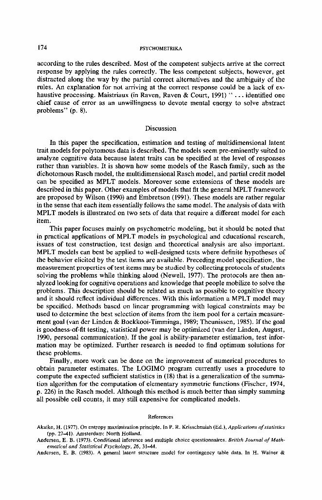
Figure 2 and 3 show two matrix items. To protect the security of the Raven problems, none of the actual items from the test are depicted here. Instead, the items are illustrated with isomorphs that use the same rules but different figural elements and

TABLE 3

Goodness-of-fit Statistics for Fitted Models

Model X 2 G 2 DF AIC

A 407.57 409.19 413 -416.81

B 968.67 931.33 473 - 14.67

C 1626.00 1790.45 491 808.45


A A A

A A A A A )

3

k)J X)JA) 5 6

rA ) I.x. ) FI~uP~ 2.

7

Isomorph of Raven matrix Item C4.

4

A) 8

LA) attributes. The numbers in the test of the actual items that were presented to the subjects are C4, C9, D7 and D9 respectively, which can be consulted by the readers.

In Figure 2 and 3 it is seen that each item has eight answer alternatives. The subject is asked to choose the picture that s(he) thinks fits the matrix best. These problems can be solved by scanning certain rules. Carpenter, Just and Shell (1990) described these rules as: (I) quantitative pairwise progression, (II) constant in a row and (III) distribution of three values. For example in Figure 2, each row contains one or more triangles. The number of triangles is constant in each row. So according to Rule II, the correct alternative should have three triangles. This then leaves alternative 3, 5, and 8 as possible candidates for the missing picture. The correct alternative can now be identified by Rule I, quantitative pairwise progression.

Quantitative pairwise progression is a quantitative increment or decrement that occurs between adjacent entries in an attribute such as size, position or number. In Item I this is the number of dots increasing in each row, so that the correct number of dots should be three as in Alternative 1, 4, and 8. Combining both rules we have Alternative 8 as the correct alternative.

Studying the interrelations among ability test scores from different data sources,

166 PSYCHOMETRIKA

O - o , , . , , i , , i )

1 2 3

d®l) )JQ) 4

lvl) 5 6 7 Illlllllllllllllll

FIGURE 3. Isomorph of Raven matrix Item C9.

Marshalek, Lohman and Snow (1983) concluded that the ability to solve matrix problems is central to analytic intelligence. The test is a pure measure of it and does not involve disturbing variables like language or declarative knowledge (Hunt, I974).

Raven himself described the abilities that he intended to measure primarily in terms of characteristics of the problem, not specific cognitive processes. This suggests that different rules might give rise to a different ability ordering of individuals. In this case we might postulate that each rule pertains to a qualitatively different ability trait so that the test responses are to be explained by a multidimensional ability space. If, on the other hand, the subjects' responses depend on the same cognitive skills regardless of the particular rule, it may be enough to postulate only one latent ability trait.

A relevant piece of research is reported by Carpenter et al. (1990). They studied subjects' eye fixations and verbal protocols while solving matrix problems and observed that

F i r s t . . . [the rules] were described one at the time . . . . Second, the induction of each rule consisted of many small steps, reflected in the pair wise comparison of elements in the adjoining en t r i e s . . . (p. 411)

HENK KELDERMAN AND CARL P. M. RIJKES

TABLE 4

Hypothesized weights of Raven Progressive Matrices Items

Model Item I Pairwise II Constant III Distribution Progression in a Row of Three Values

1 2 3 4 5 6 7 8 1 2 3 4 5 6 7 8 1 2 3 4 5 6 7 8

167

a i* 1 1 1 1 1 1 2 1 Ii II 3 1 12 ii 4 21111

b 1 1 1 1 1 1 1 2 1 12 11 3 1 12 11 4 21111

c 1 1 1 1 1 1 1 2 1 12 11 3 1 12 11 4 21111

d 1 1 1 1 1 2 1 12 11 3 1 12 i 1 4 21111

Response categories recieving a B-weight of 0 in all models are

collapsed into one category. So, for example for item 1 the response

categories 2, 6, and 7 are collapsed into one categorie.

Furthermore they remark that

One of the most notable properties of the visual scan was the row-wise organiza- tion, consisting of repeated scans of the entries in a row. There was a strong tendency to begin with a scan of the top row and to proceed downward to hori- zontally scan each of the other two rows, with only occasional look backs to a previously scanned row. (p. 425)

This makes the column-wise processing unlikely. Testing for Column-wise processing is possible, for example, in Item 1. In this item, constant in a row can be replaced by column-wise pairwise progressing and row-wise pairwise progression by "constant in a column" (see Figure 2).

To specify a MPLT model we relate each of the item responses to one or more rules and each rule to a latent ability trait. Table 4, Model a, shows hypothesized rule specifications for the responses to each of the four items.

Each number denotes the number of applications of a particular rule. Note that Item 1 and 2 involve two rules and Item 3 and 4 only one rule: "Distribution of three values". Note from Table 4 that in Item 3 and 4 the correct alternative involves the rule twice. Next, the numbers of Table 4 are used as B-weights in the MPLT model (1). For the moment we assume that each rule corresponds to one particular latent ability trait. For example for Item 2, Model a, the MPLT model becomes

168 PSYCHOMETRIKA

Table 5

Akaike's Information Criterion Statistics for Raven Data

Model Traits Loglinear Model Npar AIC DF

a I,II,III

a I I+II,III

a 2 I+III,II

a 3 I,II+III

a 4 I+II+III

O None

[l]...[4][I,II,III]

[l]...[4][I+II,III]

[l]...[4l[I+III,II]

[1]...[4][I,II+III]

[l]...[4][I+II+III]

[I]...[4]

60 866.59 1020

42 908.74 1038

38 872.79 1042

38 888.64 1042

27 912.95 1053

20 1329.97 1060

b I,II,III

c I,II,III

d I,II,III

[i]... [4] [I,II,III] 68 848.50 1012

[i]... [4] [I,II,III] 68 856.70 1012

[i]... [4] [I,II,III] 68 825.26 1012

p ( x i 2 = 1 [ 0 i ) = C21 exp [Oi~ - 8211]

p ( x i 2 = 61Of) = c21 exp [0il - ~216]

p ( x i 2 = 7[0i) = c21 exp [ ( 0 i l - - ~217) -{- ( 0 i 2 -- ~227)]

p ( x i 2 = 8101) = C2 1 exp [ 0 i 2 -- t$228]

p(xi2 = 2 or 3 o r 4 or 510i) = c21,

where c 2 is the proportionality constant, which is equal to the sum of each o f the exponentials plus one. Note that for the totally incorrect Responses 2 thru 5, the response categories are collapsed into one category in the MPLT model. This category then gets a B weight of zero. This is also done for the completely incorrect alternatives in the other items. Note further that the two item parameters 6217 and 6227 are not unique for Response 7; adding a constant c to 6217 and subtracting it from t$227 does not change the model. Therefore only their sum 6217 + 6227 is estimable.

Model a can be used as a starting point for the specification o f some more restric- tive models. To test the dimensionality of the latent space we set two or three of the latent traits or Oil o r 0i2 o r 0i3 equal to each other. Table 5 gives all models (a I thru a 4) where two or more 0 values are set equal to each other. The third column of Table 5 gives the loglinear model in concise notation: Arab numerals denote items and Roman numerals the weight sums corresponding to the latent traits. If one or more variables are between square brackets, it means that all main and interaction effects of these variables are present in the model. In the loglinear model specification [I, II + III] means that latent trait two and three are set equal to one another. In that case there is only an interaction between two sumscore variables. Model ~ is the complete inde-


Table 6

Item x Weight-sum Grouped-Goodness-of-Fit Statistics for Raven Data

Model Item Trait I Trait II Trait III

X 2 DF X 2 DF X 2 DF

1 34.03*** 9 17.05"** 4 2 9.98*** 7 17.16"** 3 3 4.85 8 4 5.66 8

1 24.28*** 9 11.18" 4 2 2.19 7 2.91 3 3 4.85 8 4 5.66 8

1 21.95"* 9 10.29" 4 2 2.85 7 .89 3 3 4.85 8 4 5.66 8

1 3.10 9 4.35 4 2 2.74 7 2.37 3 3 4.85 8 4 5.66 8

* p<.050, ** p<.010, *** p<.001

pendence model where no traits are specified. Its loglinear model has main effects of I tem 1 through 4 but no weight sum effects.

F rom the AIC values in Table 5 it is seen that the complete independence model does not explain the data as well as the other models. Fur thermore, the three-dimensional Model a has a bet ter fit than the one-dimensional Model a 4, and also a bet ter fit than the two-dimensional Models a I thru a 3 .

To test whether Model a fits the data in an absolute sense, the van den Wollenberg Q1 type statistics are computed for each of the grouped item response x weight sum contingency tables. Because the weight sum is a sufficient statistic for the latent trait, the Pearson fit statistics are sensitive to a lack of fit of the responses of an item with respect to the particular latent trait. If the fit is bad it indicates that the choice of B-weights is incorrect.

Looking at Table 6, it is seen that I tem 1 and I tem 2 have some lack of fit with respect to both weight sum I and II. Considering the specification of the B-weights, it seems that the application of the pairwise-progression rule is misspecified in I tem 2. Looking at Figure 3, it is seen that for the partially correct alternatives 1 and 6 the pairwise progression rule can be applied to the position of the dot with respect to the small ellipse whereas in the correct alternative 7, the pairwise-progression rule can also be applied to the small ellipse in relation to the larger ellipse. Therefore it can be argued that the B-weight o f Response 7 with respect to Rule I should be 2 rather than 1. Making

170 PSYCHOMETRIKA

4 -

3 -

2-

1-

O-

-1-

response 1

0 response 3

response 4

response 5

m response 8

response 0

-2-

1 2 3

Weightsum I FIGURE 4.

Pearson residuals for responses of Item 1 against Weight Sum I.

this change gives Model b (see Table 4). In Table 6 it can be seen that the fit of item 2 in Model b has now become quite satisfactory, but the fit of Item I is still bad.

Considering the specification of Item 1, we cannot see a priori reasons to change the size of any weights. One possibly different specification for Item 1 has been discussed before, column-wise processing rather than row-wise. In the columns, the number of dots is constant. Using the constant-in-a-column rule, Alternative 1, 4, and 8 become partially correct alternatives. Likewise the number of triangles can be obtained by applying pairwise progression in column-wise way, giving 3, 5 and 8 as possible answers. In Model c the B-weights of Item I are changed in such a way that they are in accordance with column-wise processing. It is seen in Table 6, however, that Item 1 still has no good fit to the data.

Because no further a priori reasons could be found to propose a different model for Item I, it was decided to look at the residuals of this item. In Figure 4 and 5, the Pearson residuals for the six responses of Item I are plotted against the weight sum I and II respectively. Looking at Figure 4, it seems that Response I does not fit the data very well. More responses than expected are given for low values of the weight sums and less responses are given for high values of the weight sums. This is an indication of a scoring weight of Response 1 that is specified too large. A plot against weight sum II (see Figure 5) gives a similar picture. From Figure 4 and 5 we can also notice a slight overspecification of Response 5. The frequencies of occurrence of the partial Re- sponses 1 and 5 (17 and 24) are also considerably lower than those of the partial Responses 3 and 4 (151 and 169).

There are two visual differences of Response I and 5 when compared with Re-


2,5 - -

2

1.5

1

0 . 5 -

0 -

-0.5 -

"1 - -

-1.5 -

- 2 -

\

0 1 2

[ ] response 1

0 response 3

response 4

- 0 - " response 5

,..,~ response 8

'~ response 0

Weightsum II FIGURE 5.

Pearson residuals for responses of Item 1 against Weight Sum II.

sponse 3 and 4. The first concerns the complexity of the responses. This does not show itself in Figure 1, but is clear in the original item C4. Response 3 and 4 both have 25% more figure elements in the picture than Response 1 and 5 (the correct Response 8 has 50% more). Forbes (1964) noted that: "A person of greater intellectual ability adopted the principle that the most complex figure must be the right one, or adopted some more or less arbitrary method of reasoning" (p. 232). This may account for the greater attractiveness of Responses 3 and 4. The second difference concerns the location of the response in the matrix. Response 3 and 4 are adjacent to the missing entry whereas Response 1 and 5 are not. On the influence of this adjacency on the subjects response, Hunt (1974) remarked that: "We have no theory to guide us here, but empirical observations of error patterns in Set II problems [of the Raven test] Forbes (1964) suggest that the elements adjacent to the m33 element [the missing entry] (i.e., m32 or m23) should be used. [are more attractive]" (p. 141).

From these observations, it is hypothesized that the weights of Response 1 and 5 are zero rather than one. In this way Model b is changed into Model d. It is seen from Table 6 that all four items have a good fit in Model d. Also model d has the smallest AIC value (see Table 5). The overall Pearson and likelihood-ratio goodness-of-fit statistics may not be used because there are too many small expected frequencies (e.g., 0.03) and they differ too much in size (e.g., 0.03 and 62.00). As remarked earlier, in these cir- cumstances it can be expected from Koehler (1986, Table 3) that, the likelihood-ratio statistic (G 2) is probably too liberal and the Pearson goodness-of-fit statistic (X 2) too conservative. For model d this is confirmed, G 2 and X 2 are 689 and I 119 respectively on 1012 degrees of freedom, so that G 2 indicates a fit too good to be true (p = .99) and

172 PSYCHOMETRIKA

TABLE 7

Phi Parameter Estimates (and Standard Errors) of Model d

Response I t em

1 2 3 4

(.27) + (.12) 1 -1.47

2 0.001

3 1.493

4 1.702

5 -1.13

6 0.001

7 0.001

8 3.944

.14

.14

.23

.13

1.222 0.001

0.001 1.416

0.001 0.001

0.001 1.856

0.001 4,347

0.462 (.14) 0.001

3.,505 (.i0) 0.326

0.643 (.16) 1.596

3.457*

.15) 0.546

1.136

.13) 0.856

.ii) 0.736

0.001

(.21) 0.001

(.14) 0.001

(.09)

(.14)

(.12)

(.13)

(.13)

The correct answer is underlined

÷ Standard errors are between brackets.

1 Incorrect categories collapsed, parameter fixed at zero

2 _Sjlx ' 3 _Sj2x ' 4 _(Sjl x ÷ 8j2x), 5 _(28jlx ÷ ~j2x),

6-~j3x, 7 _2~j3 x

X 2 a bad fit (p = .01). From the Q1 type statistics in Table 6, however , we can conclude that model d has an acceptable fit to the data and must be preferred to the other models.

Table 7 shows the LOGIMO estimates of the dpj x parameters of Model d. The 4, parameters for the incorrect parameters are set to zero so that the 4, parameters can easily be related to the ~ parameters in the following way:

~bjx = --BjL~ if BjL~ = 1, Bj2~ = O, Bj3~ = O,

q~jx = - ( 2 8 j l x + 8j2x) if Bjtx = 2, Bj2,: = 1, Bjax = O,

~bjx = -~j2x if Bjlx = O, By2x = 1, njax = O,

'bjx = - ( 6 j t x + 6j2x) if Bjlx = 1, Bj2x = 1, Bj3x = O,

Ckjx = -S j3x if Bjlx = O, Bj2x = O, Bj3x = 1,

~bjx = -2Bj3x if Bjlx = O, Bjz~ = O, Bj3x = 2,

Comparing the alp-parameters of the items we can see from Table 7 that Item 3 is easier than Item 4. Looking within the items we can see that for all items the partial correct answers are more attractive than the incorrect response categories.

A convenient w a y to interpret the item parameters is to look at a graphical repre- sentation of the item characteristic function (ICF). For example, in Figure 6 three


~ 0

0 0 -"-...ff I0 - 2 0

(b)

P o.~ o.

o

-20 e~

1 i ~ P 0 . 7 5 ~ 0 . 5 0.25

0 -2~ ~

-10 O,

o °

-20 ~ O,

F~ 10

(a)

i

0 10

(c)

i0 -20

(e)

Oo bTs~ 10

0

0

10 -20

(d)

FIGURE 6. Three dimensional plot of the Item Characteristic Function of Item 2 for: (a) the incorrect response categories 2, 3, 4 and 5; (b) the partial correct response category 1; (c) the partial correct response category 6; (d) the partial correct response category 8; (e) the correct response category (7).

dimensional plots of the ICFs of the different response categories of Item 2 are given. The axes in the horizontal plane correspond with the latent traits 01 (in the front) and 02 (in the back) that are related to the quantitative pairwise progression and constant-in- a-row rule respectively. The vertical axe gives the probability for the given response category for different values of 0t and 0 2 .

Figure 6a corresponds with the incorrect response Categories 2, 3, 4 and 5. Sub- jects with low 01 and 0z values have a high probability of choosing one of these categories. Figure 6b and Figure 6c correspond to the partial correct Alternatives 1 and 6 respectively. Subjects with a high 01-value and a low 0z-value are likely to choose category 1, and to a lesser extent category 6. On the other hand, subjects with a low 01-value and a high 0z-value are likely to choose the partial correct Alternative 8 (Figure 6d). Finally, only those subjects that have a high 01-value and a high 0z-value have a high probability of choosing the correct Response 7 (Figure 6e). Notice also from Figure 6e the steep climbing of the ICF in the 01 -direction due to the heavier B-weight for the 01 -dimension. Similar kind of plots and interpretations can be given for the other items.

The pattern described above might be expected when subjects solve the items

174 PSYCHOMETRIKA

according to the rules described. Most of the competent subjects arrive at the correct response by applying the rules correctly. The less competent subjects, however, get distracted along the way by the partial correct alternatives and the ambiguity of the rules. An explanation for not arriving at the correct response could be a lack of ex- haustive processing. Maistriaux (in Raven, Raven & Court, 1991) " . . . identified one chief cause of error as an unwillingness to devote mental energy to solve abstract problems" (p. 8).

Discussion

In this paper the specification, estimation and testing of multidimensional latent trait models for polytomous data is described. The models seem pre-eminently suited to analyze cognitive data because latent traits can be specified at the level of responses rather than variables. It is shown how some models of the Rasch family, such as the dichotomous Rasch model, the multidimensional Rasch model, and partial credit model can be specified as MPLT models. Moreover some extensions of these models are described in this paper. Other examples of models that fit the general MPLT framework are proposed by Wilson (1990) and Embretson (1991). These models are rather regular in the sense that each item essentially follows the same model. The analysis of data with MPLT models is illustrated on two sets of data that require a different model for each item.

This paper focuses mainly on psychometric modeling, but it should be noted that in practical applications of MPLT models in psychological and educational research, issues of test construction, test design and theoretical analysis are also important. MPLT models can best be applied to well-designed tests where definite hypotheses of the behavior elicited by the test items are available. Preceding model specification, the measurement properties of test items may be studied by collecting protocols of students solving the problems while thinking aloud (Newell, 1977). The protocols are then analyzed looking for cognitive operations and knowledge that people mobilize to solve the problems. This description should be related as much as possible to cognitive theory and it should reflect individual differences. With this information a MPLT model may be specified. Methods based on linear programming with logical constraints may be used to determine the best selection of items from the item pool for a certain measurement goal (van der Linden & Boekkooi-Timminga, 1989; Theunissen, 1985). If the goal is goodness-of-fit testing, statistical power may be optimized (van der Linden, August, 1990, personal communication). If the goal is ability-parameter estimation, test information may be optimized. Further research is needed to find optimum solutions for these problems.

Finally, more work can be done on the improvement of numerical procedures to obtain parameter estimates. The LOGIMO program currently uses a procedure to compute the expected sufficient statistics in (18) that is a generalization of the summation algorithm for the computation of elementary symmetric functions (Fischer, 1974, p. 226) in the Rasch model. Although this method is much better than simply summing all possible cell counts, it may still expensive for complicated models.

References

Akaike, H. (1977). On entropy maximization principle. In P. R. Krisschnaiah (Ed.), Applications of statistics (pp. 27-41). Amsterdam: North Holland.

Andersen, E. B. (1973). Conditional inference and multiple choice questionnaires. British Journal of Math- ematical and Statistical Psychology, 26, 31-44.

Andersen, E. B. (1983). A general latent structure model for contingency table data. In H. Walner &

HENK KELDERMAN AND CARL P, M, RIJKES 175

S. Messick (Eds.), Principals of modern psychological measurement (pp. 117-138). Hillsdale, NJ: Lawrence Erlbaum.

Andrich, D. (1978). A rating scale formulation for ordered response categories. Psychometrika, 43, 561-573. Andrich, D. (1982). An extension of the Rasch model for ratings providing both location and dispersion

parameters. Psychometrika, 47, 105-113. Baglivo, J., Olivier, D., & Pagano, M. (1992). Methods for exact goodness-of-fit tests, Journal of the Amer-

ican Statistical Association, 87, 464-469. Bishop, Y. M. M., Fienberg, S. E., & Holland, P. W. (1975). Discrete multivariate analysis. Cambridge, MA:

MIT Press. Bock, R. D. (1972). Estimating item parameters and latent ability when responses are scored in two or more

nominal categories. Psychometrika, 37, 29-51. Carpenter, P. A., Just, M. A., & Shell, P. (1990). What one intelligence test measures: A theoretical account

of the processing in the Raven Progressive Matrices Test. Psychological Review, 97, 404-431. Cox, M. A. A., & Placket, R. L. (1980). Small samples in contingency tables. Biometrika, 67, 1-13. Cressie, N., & Holland, P. W. (1983). Characterizing the manifest probabilities of latent trait models. Psy-

chometrika, 48, 129-142. de Leeuw, J., & Verhelst, N. D. (1986). Maximum likelihood estimation in generalized Rasch models.

Journal o f Educational Statistics, 11, 183-196. Duncan, O. D. (1984). Rasch measurement: Further examples and discussion. In C. F. Turner & E. Martin

(Eds.), Surveying subjective phenomena, Vol. 2 (pp. 367--403), New York: Russell Sage Foundation. Duncan, O. D., & Stenbeck, M. (1987). Are Likert scales unidimensional? Social Science Research, 16,

245-259. Embretson, S. E. (1984). A general latent trait model for response processes. Psychometrika, 49, 175-186. Embretson, S. E. (1985). Multicomponent latent trait models for test design. In S. E. Embretson (Ed.), Test

design: Developments in psychology and psychometrics (pp. 195-218). Orlando, FL: Academic Press. Embretson, S. E. (1991). Measuring and validating the cognitive modifiability construct. Poster Presentation

at the Annual Meeting of the American Educational Research Association. Fischer, G. H. (1972). A measurement model for the effect of mass-media. Acta Psychologica, 36, 207-220. Fischer, G. H. (1973). The linear logistic test model as an instrument in educational research. Acta Psycho-

logica, 36, 359-374. Fischer, G. H. (1974). Einfiihrung in die Theorie psychologischer Tests [Introduction to the theory of psy-

chological tests]. Bern: Huber (In German). Fischer, G. H. (1976). Some probabilistic models for measuring change. In D. N. M. de Gruyter & L. J. Th.

van der Kamp (Eds.), Advances in psychological and educational measurement (pp. 97-110). New York: Wiley.

Fischer, G. H., & Forman, A. K. (1982). Some applications of logistic latent trait models with linear constraints on the parameters. Applied Psychological Measurement, 6, 397--416.

Forbes, A. R. (1964). An item analysis of the advanced matrices. British Journal of Educational Psychology, 34, 1-14.

Frederiksen, J. R. (1982). A componential theory of reading skills and their interactions. In R. J. Sternberg (Ed.), Advances in the psychology of human intelligence Vol. 1 (pp. 125-180). Hillsdale, NJ: Lawrence Erlbaum.

Glas, CA. W., & Verhelst, N. D. (1989). Extensions of the Partial Credit Model. Psychometrika, 54, 635--660. Haberman, S. J. (1977). Log-linear models and frequency tables with small cell counts, Annals o f Statistics,

5, 1124-1147. Haberman, S. J. (1979). Analysis of qualitative data: New developments, Vol. 2. New York: Academic Press. Hunt, E. B. (1974). Quote the Raven? Nevermore! In L. W. Greg (Ed.), Knowledge and cognition (pp.

129-158). Hillsdate, NJ: Lawrence Erlbaum. Imrey, P. B., Koch, G. C., & Stokes, M. E. (1981). Categorical data analysis: Some reflections on the

toglinear model and logistic regression. Part I: Historical and methodological overview. International Statistical Overview, 49, 265-283.

Kelderman, H. (1984). Loglinear Rasch model tests. Psychometrika, 49, 223-245. Kelderman, H. (1989). Item bias detection using loglinear IRT. Psychometrika, 54, 681-697. Kelderman, H. (1992). Computing maximum likelihood estimates of loglinear IRT models from marginal

sums. Psychometrika, 57, 437--450. Kelderman, H., & Steen, R. (1988). Logimo: Loglinear IRT modeling [program Manual]. Enschede, The

Netherlands: University of Twente. Koehler, K. J. (1977). Goodness-of-fit statistics for large sparse multinomials. Unpublished doctoral disser-

tation, University of Minnesota, School of Statistics. Koehler, K. J. (1986). Goodness-of-fit tests for log-linear models in sparse contingency tables. Journal of the

American Statistical Association, 81,483-493.

176 PSYCHOMETRIKA

Lancaster, H. O. (1961). Significance tests in discrete distributions. Journal of the American Statistical Association, 56, 223-234.

Lehmann, E. L. (1983). The theory of point estimation. New York: John Wiley. Marshalek, B., Lohman, D. F., & Snow, R. E. (1983). The complexity continuum in the radex and hierar-

chical models of intelligence. Intelligence, 7, 107-127. Masters, G. N. (1982). A Rasch model for partial credit scoring. Psychometrika, 47, 149-174. Muraki, E. (1990). Fitting a polytomous item response model to Likert type data. Applied Psychological

Measurement, 14, 59-71. Newell, A. (1977). On the analysis of human problem solving protocols. In P. N. Johnson-Laird & P. C.

Wason, Thinking (pp. 46--61). London: Cambridge University Press. Neyman, J., & Scott, E. L. (1948). Consistent estimates based on partially consistent observations. Econo-

metrica, 16, 1-32. Rao, C. R. (1973). Linear statistical inference and its applications. New York: Wiley. Rasch, G. (1961). On general laws and the meaning of measurement in psychology. Proceedings of the fourth

Berkeley symposium on mathematical statistics and probability (pp. 321-333). Berkeley, CA: University of California Press.

Rasch, G. (1980). Probabilistic models for some intelligence and attainment tests. Chicago: The University of Chicago Press.

Raven, J., Raven, J. C., & Court, J. H. (1991). Manual for Raven's progressive matrices and vocabulary scales (section 1): General overview. Oxford: Oxford Psychologists Press.

Read, T. R. C., & Cressie, N. (1988). Goodness-of-fit statistics for discrete multivariate data. New York: Springer-Vedag.

Rost, J. (1988). Measuring attitudes with a threshold model drawing on a traditional scaling concept. Applied Psychological Measurement, 12, 397--409.

Samejima, F. (1972). A general model for free-response data. Psychometrika Monograph No. 18, 37 (4, Pt. 2).

Scheiblechner, H. (1972). Das lernen und Ibsen komplexer Denkaufgaben [Learning and solving complex cognitive problems]. Zeitschrift fiir experimentelle und Angewandte Psychologie, 19, 476-506. (In Ger- man)

Spada, H. (1976). Modelle des Denkens und Lernens [Models of thinking and learning]. Bern: Huber. (In German)

Stenner, A. J., Smith, III, M., & Burdick, D. (1983). Toward a theory of construct definition. Journal of Educational Measurement, 20, 303-316.

Sternberg, R. J. (Ed.). (1982). Advances in the psychology of human intelligence, Vol. 1. Hillsdale, NJ: Lawrence Erlbaum.

Thissen, D., & Steinberg, L. (1984). A response model for multiple choice items. Psychometrika, 49, 501- 519.

Theunissen, T. J. J. M. (1985). Binary programming and test design. Psychometrika, 50, 411-420. Tjur, T. (1982). A connection between Rasch's item analysis model and a multiplicative Poisson model.

Scandinavian Journal of Statistics, 9, 23-30. van den Wollenberg, A. L. (1982). Two new test statistics for the Rasch model. Psychometrika, 47, 123-140. van der Linden, W. J., & Boekkooi-Timminga, E. (1989). A maximum model for test design with practical

constraints. Psychometrika, 54, 237-248. Wilson, M. (1989). The partial order model. Paper presented at the Fifth International Objective Measure-

ment Workshop, Berkeley, CA. Wilson, M. (1990). An extension of the partial credit model to incorporate diagnostic information. Unpub-

lished manuscript, University of California, Graduate School of Education, Berkeley, CA. Wright, B. D., & Masters, G. N. (1982). Rating scale analysis. Chicago: MESA Press.

Manuscript received 10/19/88 Final version received 11/18/92

Documents

Loglinear multidimensional IRT models for polytomously