Logarithmic scaling in the longitudinal velocity variance explained by a spectral budgetT. Banerjee and G. G. Katul Citation: Physics of Fluids (1994-present) 25, 125106 (2013); doi: 10.1063/1.4837876 View online: http://dx.doi.org/10.1063/1.4837876 View Table of Contents: http://scitation.aip.org/content/aip/journal/pof2/25/12?ver=pdfcov Published by the AIP Publishing

This article is copyrighted as indicated in the article. Reuse of AIP content is subject to the terms at: http://scitation.aip.org/termsconditions. Downloaded to IP:

152.3.111.38 On: Tue, 10 Dec 2013 18:31:41

PHYSICS OF FLUIDS 25, 125106 (2013)

Logarithmic scaling in the longitudinal velocity varianceexplained by a spectral budget

T. Banerjeea) and G. G. Katulb)

Nicholas School of the Environment, Box 90328, Duke University, Durham,North Carolina 27708, USA

(Received 5 September 2013; accepted 18 November 2013;published online 10 December 2013)

A logarithmic scaling for the streamwise turbulent intensity σ 2u /u∗2 = B1 − A1

ln (z/δ) was reported across several high Reynolds number laboratory experiments aspredicted from Townsend’s attached eddy hypothesis, where u∗ is the friction velocityand z is the height normalized by the boundary layer thickness δ. A phenomenologicalexplanation for the origin of this log-law in the intermediate region is provided herebased on a solution to a spectral budget where the production and energy transferterms are modeled. The solution to this spectral budget predicts A1 = (18/55)Co/κ2/3

and B1 = (2.5)A1, where Co and κ are the Kolmogorov and von Karman constants.These predictions hold when very large scale motions do not disturb the k−1 scalingexisting across all wavenumbers 1/δ < k < 1/z in the streamwise turbulent velocityspectrum Eu(k). Deviations from a k−1 scaling along with their effects on A1 andB1 are discussed using published data and field experiments. C© 2013 AIP PublishingLLC. [http://dx.doi.org/10.1063/1.4837876]

I. INTRODUCTION

Scaling-laws and self-similar states remain the cornerstone of turbulence research, especiallyin the so-called intermediate region of wall bounded flows where production and dissipation ofturbulent kinetic energy (TKE) are in balance and spectrally separated, the Kolmogorov inertialsubrange theory describes the local structure of the velocity statistics, and the von Karman-Prandtllogarithmic law describes the mean velocity (U ) given by

U+ = 1

κlog(z+) + Aw, (1)

where U+ = U/u∗ is the normalized mean longitudinal velocity, z and z+ = zu∗/ν are, respectively,the distance and normalized distance from the wall, u∗ = √

τt/ρ f is the friction (or shear) velocity,κ is the von Karman constant, Aw is a wall constant, τ t is the turbulent stress assumed independentof z in the intermediate region, ν and ρ f are the fluid kinematic viscosity and density, respectively,and over-line designates time-averaging. The logarithmic profile shape for U+ in the intermediateregion has been supported by a myriad of studies,1–8 including Townsend’s attached eddy hypothesis.Besides propounding the log-law for U , Townsend’s attached eddy hypothesis has also predicteda logarithmic scaling for the streamwise turbulence intensity (u′2), defined as the mean squaredquantity of the streamwise turbulent velocity fluctuations of the following form:6, 8, 9

u2+ = B1 − A1 log(z/δ), (2)

where u2+ = u′2/u∗2, the normalized longitudinal velocity variance in wall units and δ is the

thickness of the turbulent boundary layer. This result has lacked robust experimental support exceptfrom a few studies7, 10–13 until recently. Significant interest has been noticed about the topic in

a)Electronic mail: tirtha.b@duke.edub)Electronic mail: gaby@duke.edu

1070-6631/2013/25(12)/125106/13/$30.00 C©2013 AIP Publishing LLC25, 125106-1

This article is copyrighted as indicated in the article. Reuse of AIP content is subject to the terms at: http://scitation.aip.org/termsconditions. Downloaded to IP:

152.3.111.38 On: Tue, 10 Dec 2013 18:31:41

125106-2 T. Banerjee and G. G. Katul Phys. Fluids 25, 125106 (2013)

recent years following publications by Smits, McKeon, and Marusic,14 Marusic et al.,8 and Smitsand Marusic15 where four different experiments at very high Reynolds numbers were compiled toillustrate the universality of Eq. (2) across a wide range of bulk Reynold’s number.8, 16–19 The compassof this work is to provide a phenomenological explanation to Eq. (2) based on a spectral budget ofthe longitudinal velocity thereby offering another perspective on the origin of its logarithmic (orpower-law) character. Specifically, a k−1 scaling at low wavenumbers (k) for the streamwise turbulentvelocity spectrum (Eu(k)) has been prevalent in turbulence literature for some time7, 10, 11, 20–42 both forwall bounded flows and atmospheric surface layer turbulence. Those studies differ in predicting theextent of the k−1 scaling at low k. One study even found a prevalent k−1 scaling and a limited inertialsubrange for z+ ∈ [220 − 890].43 The arguments resulting in a k−1 scaling range from a theoreticalspectral budget analysis20, 21, 26 to dimensional analysis32 to laboratory and field experiments.29, 39

Townsend’s attached eddy hypothesis has also been used in the interpretation of the aforesaid k−1

scaling in a few studies.31 In Nikora,42 a k−1 scaling has been explained in the range 1/H ≤ k ≤1/z as a result of superimposition of eddy cascades44 generated at all possible distances from thewall, where H = αδ is the external length scale proportional to the boundary layer thickness viaa coefficient α. A few studies have not observed a clear k−1 scaling45–47 and others have foundthe existence only under certain constraints.48 Another phenomenological explanation has beenproposed by Katul, Porporato, and Nikora49 that bridges some of the mechanisms explaining the k−1

power law scaling at low k in the turbulent kinetic energy spectrum Etke(k) using simplifications toTchen’s20, 21 spectral budget, Nikora’s42 phenomenological scaling for the dissipation rate spectrum,and Heisenberg’s50 eddy viscosity. However, a spectral budget approach lacking any accounting fora rigid boundary remains problematic.14, 51, 52 In the present study, an explicit production term thataccounts for the mean velocity gradient and a break-point in the vertical velocity spectra at z areused to supplement a spectral budget leading to the k−1 scaling, which is then used to explain the

log-law of u2+

, including a link between the Kolmogorov constant, the parameters A1 and B1, andthe proportionality coefficient α.

II. THEORY

A. Definitions and general considerations

The Reynolds-averaged TKE budget equation (without buoyancy or rotational accelerationterms) is given by53

∂e

∂t+ U j

∂e

∂x j= −ui

′u j′ ∂Ui

∂x j− ∂(u j

′e)

∂x j− 1

ρ f

∂(ui′ P ′)

∂xi− ε, (3)

where x1 = x, x2 = y, and x3 = z are the longitudinal, lateral, and vertical directions, respectively, U1

= U, U2 = V , and U3 = W are the mean longitudinal, lateral, and vertical velocity components, ui′

are turbulent velocity excursions around Ui, e = 12

(σ 2

u + σ 2v + σ 2

w

)is the TKE, σ 2

u = u′2, σ 2v = v′2,

and σ 2w = w′2 are the root-mean-squared velocity component along directions xi, respectively, and

the coordinate system xi is aligned so that x1 is along the U direction with W = V = 0. The first andsecond terms on the left-hand side of Eq. (3) represent local storage and advection of e by the meanflow. On the right hand side, the first term indicates mechanical or shear production of TKE due to afinite mean velocity gradient, the second and third terms represent transport of TKE by turbulenceand pressure-velocity interactions, respectively, and the last term indicates viscous dissipation ofTKE. As is the case with laboratory studies, assuming stationary and planar-homogeneous flowresults in Refs. 53 and 54

∂e

∂t= 0 = −u′w′ dU

dz− ∂

∂z

(w′e + w′ p′) − ε, (4)

where u′w′ = −u2∗ is the mean momentum flux. It is to be noted that p′ in Eq. (4) is normalized

by ρ f . In the intermediate region of boundary-layers, the transport terms are usually small resultingin a near-balance between production and dissipation of TKE as assumed by Townsend and manyothers.5, 54

This article is copyrighted as indicated in the article. Reuse of AIP content is subject to the terms at: http://scitation.aip.org/termsconditions. Downloaded to IP:

152.3.111.38 On: Tue, 10 Dec 2013 18:31:41

125106-3 T. Banerjee and G. G. Katul Phys. Fluids 25, 125106 (2013)

B. A spectral budget

If ε is a conservative quantity in the turbulent energy cascade, then a simplified spectral budgetrepresenting the interplay between the same terms in Eq. (4) can be derived for any wavenumber kas23, 26

ε = −dU

dz

∞∫k

Fwu(p)dp + FT R(k) + 2ν

k∫0

p2 Etke(p)dp, (5)

where the first, second, and third terms represent the production of TKE in the range of [k, ∞],the transfer of TKE in the range [k, ∞], and the viscous dissipation in the range of [0, k]. Twoasymptotic conditions must be satisfied so that this spectral budget recovers its Reynolds-averagedTKE counterpart. The first is that at k = 0, FTR(0) = 0, and

ε = −dU

dz

∞∫0

Fwu(p)dp = −dU

dz

(u′w′) , (6)

so that∞∫0

Fwu(p)dp = u′w′ to ensure a balance between mechanical production and ε is maintained

in the intermediate region. The second is that as k → ∞, FTR(∞) → 0, and

ε ≈ 2ν

∞∫0

p2 Etke(p)dp, (7)

or ε is primarily explained via the viscous term at very large k. The Fwu(k) that is related to theproduction term, and the FTR(k) that is related to the action of the triple moments and pressure-velocity interactions both require closure.

In deriving closure expressions for Fwu(k) and FTR(k), Etke(k) is related to the spectra of theindividual velocity components by

Etke(k) = 1

2[Eu(k) + Ev(k) + Ew(k)] , (8)

and for kz > 1, these component-wise velocity spectra can be described by the Kolmogorov44 scaling(hereafter referred to as K41) given as

Etke(k) = Coε2/3k−5/3; Ew(k) = C ′

K ε2/3k−5/3; Ev(k) = C ′K ε2/3k−5/3; Eu(k) = C ′′

K ε2/3k−5/3,

(9)where C ′

K = (24/55)CK , C ′′K = (18/55)CK , CK ≈ 1.55 is the Kolmogorov constant associated with

three-dimensional wavenumbers, and Co = (33/55)CK. Exponential (or Pao type) adjustments54

to these individual spectra as kη → 1 are momentarily ignored, where η = (ν3/ ε

)1/4is the Kol-

mogorov micro-scale, and ν is the kinematic viscosity of the fluid. Throughout, k is interpreted asone-dimensional cut along the streamwise direction x and this interpretation is adopted hereafter asinvoked when converting the time domain to the wavenumber domain using Taylor’s frozen turbu-lence hypothesis55 in experiments. Last, because the TKE and the component-wise velocity spectraare known for kz > 1 given by their K41 scaling, it is convenient to consider the spectral budget inEq. (5) at ka = 1/z instead of any arbitrary k.

C. Modeling the production term Fwu(k)

The Fwu(k) can be obtained via a co-spectral budget similar in form to the spectral budget abovegiven by56

∂ Fwu(k)

∂t+ 2νk2 Fwu(k) = Pwu(k) + Twu(k) + π (k), (10)

This article is copyrighted as indicated in the article. Reuse of AIP content is subject to the terms at: http://scitation.aip.org/termsconditions. Downloaded to IP:

152.3.111.38 On: Tue, 10 Dec 2013 18:31:41

125106-4 T. Banerjee and G. G. Katul Phys. Fluids 25, 125106 (2013)

where Pwu(k) = (dU/dz)Ew(k) is the production term, Twu(k) is the co-spectral flux-transport term,and π (k) is the velocity-pressure interaction term. Considering the co-spectral transfer term Twu(k),it is reasonable to assume that it may be small compared to the other terms given that its integral overk is ∂w′u′w′/∂z which is known to be minor in the intermediate region.57, 58 With these assumptions,the dominant terms in the co-spectral budget that remain in stationary flows are

dU

dzEw(k) + π (k) − 2νk2 Fwu(k) ≈ 0. (11)

In second-order closure modeling, the integral of π (k), Ruw, is expressed as

Ruw = −CR1

τ

(u′w′) + C2σ

2w

dU

dz, (12)

where τ = e/ε is a relaxation time scale, CR ≈ 1.8 is the Rotta constant, and C2 = 3/5 is a constantassociated with isotropization of the production term correcting the original Rotta model54, 59 andshown to be consistent with Rapid Distortion Theory.54 If the Rotta model is further invoked for thespectral version of this term, then it follows that56

π (k) = −CRFwu(k)

τ (k)+ C2 Pwu(k), (13)

where τ (k) = ε−1/3k−2/3 becomes a wavenumber dependent relaxation time scale60 assumed to varyonly with k and ε for consistency with K41. With this approximation for π (k), the co-spectral budgetreduces to56

2νk2 Fwu(k) = (1 − C2)dU

dzEw(k) − CR

Fwu(k)

τ (k). (14)

The relative importance of the Rotta component and the viscous term 2νk2 Fwu(k) can be evaluatedand is given as56

2νk2 Fwu(k)

CR Fwu(k)/τ (k)= 2

CR

(ν3k4

ε

)1/3

≈ (kη)4/3, (15)

Provided kη 1, de-correlation between u′ and w′ due to viscous effects can be ignored relativeto the Rotta term. However, it is to be noted that as kη � 1, the two terms become comparable inmagnitude, but at such fine scales, |Fwu(k)| is sufficiently small so that ignoring contributions tothe turbulent stress can be justified. With the two remaining terms describing a balance betweenproduction and pressure-velocity interaction (i.e., destruction), the co-spectral budget is now givenby56

Fwu(k) = 1

A

dU

dzε−1/3 Ew(k) k−2/3, (16)

where A = CR/(1 − C2) ≈ 4.5. For η k−1 ≤ z, then

Fwu(k) = C ′K

Aε

13 k− 7

3 . (17)

This expression agrees with Fwu(k) = Cuw(dU/dz)ε1/3k−7/3 derived from dimensionalconsiderations60, 61 and supported by a large corpus of measurements in high Reynolds numberpipe, boundary layer, and atmospheric flows.54, 62, 63 Also, the Cuw = C ′

K /A ≈ 0.65/4.5 = 0.15,agrees with the accepted value.54, 64 With such a closure model for Fwu(k),

dU

dz

∞∫ka

Fwu(p)dp = −3

4

(dU

dz

)2

Cuwε1/3k−4/3a . (18)

This completes the estimation of the production term in the spectral budget.

This article is copyrighted as indicated in the article. Reuse of AIP content is subject to the terms at: http://scitation.aip.org/termsconditions. Downloaded to IP:

152.3.111.38 On: Tue, 10 Dec 2013 18:31:41

125106-5 T. Banerjee and G. G. Katul Phys. Fluids 25, 125106 (2013)

D. Modeling the transport term FTR(k)

The Heisenberg model50 can be used to achieve a closure to FTR(k) and is given by

FT R(k) = νt (k)|curl u|2 ≈ 2νt (k)

k∫0

p2 Etke(p)dp, (19)

where u is a “macro-scale” component of the velocity, and ν t(k) is referred to as the Heisenberg50

eddy viscosity. It is produced by the motion of eddies with wavenumbers greater than k and is givenby

νt (k) = CH

∞∫k

√Etke(p)

p3dp, (20)

where CH is the Heisenberg constant. The turbulent viscosity can be evaluated as

νt (ka) = CH

∞∫ka

√Coε

2/3 p−5/3

p3dp = 3CH C1/2

o ε1/3

4k4/3a

, (21)

so that the ratio of turbulent to molecular viscosity is given by

νt (ka)

ν= 3CH C1/2

o

4(kaη)4/3. (22)

Because it is assumed that kaη 1, ν ν t(ka), and molecular effects can be ignored (as was thecase in the co-spectral budget).

E. Solving the spectral budget

If U follows Eq. (1), then dU/dz = u∗/(κz) and ε = u2∗dU/dz = u3

∗/(κz), and using Fwu(k)from Eq. (18), ν t from Eq. (21), with ν t(ka) ν simplifies the spectral budget in Eq. (5) to

ka∫0

p2 Etke(p)dp = u2∗

z2Cb, (23)

where

Cb = 2

3CH C1/2o

−(3/4) Cuw + κ4/3

κ2. (24)

To solve for Etke(k) in Eq. (23) for kz < 1, assume Etke(k) = a1kb1 thereby reducing Eq. (23) to

a1z−3−b1

3 + b1= u2

∗z2

Cb. (25)

Upon using polynomial matching, −3 − b1 = −2 or b1 = −1, and a1 = 2Cbu2∗. This analy-

sis suggests that Etke(k) = CT K E u2∗k−1, thereby recovering the −1 power-law in the spectrum

of TKE, where CTKE = 2Cb. To link Etke(k) to Eu(k), consider its definition in Eq. (8). For kz 1, Eu(k) + Ev(k) Ew(k) (generally, Ew(k) ∼ k0 for kz < 1 as discussed elsewhere54, 56).Figure 1 shows measured Eu(k), Ev(k), and Ew(k) (in regular and pre-multiplied form) computedusing orthonormal wavelet transforms (OWT) providing some experimental support to the simplifi-cation Eu(k), Ev(k) Ew(k) for kz < 1. Also at low wavenumbers, Eu(k) scales with Ev(k) so thatEu(k) = βEtke(k) = βCT K E u2

∗k−1 = C ′T K E u2

∗k−1, where β is a proportionality constant the roleof which is discussed in the Appendix and C ′

T K E = β CT K E . The OWT is used here (instead ofFourier spectra) because the wavelet coefficients are less sensitive to possible non-stationarity in thecomponent-wise velocity series. These measurements were collected at 10 Hz using a triaxial sonicanemometer positioned at z = 39.5 m above the ground surface on a meteorological tower situated

This article is copyrighted as indicated in the article. Reuse of AIP content is subject to the terms at: http://scitation.aip.org/termsconditions. Downloaded to IP:

152.3.111.38 On: Tue, 10 Dec 2013 18:31:41

125106-6 T. Banerjee and G. G. Katul Phys. Fluids 25, 125106 (2013)

10−2

100

102

10−4

10−2

100

102

104

Eu/(

z u

*2 )

kz10

−210

010

210

−4

10−2

100

102

104

Ev/(

z u

*2 )

kz10

−210

010

210

−4

10−2

100

102

104

Ew

/(z

u*2 )

kz

HW1HW2HW3−1−5/3

10−2

10−1

100

101

0

0.5

1

1.5

kEu/(

u*2 )

kz10

−210

−110

010

10

0.5

1

1.5kE

v/(u

*2 )

kz10

−210

−110

010

10

0.5

1

1.5

kEw

/(u

*2 )kz

(a) (b) (c)

(d) (e) (f)

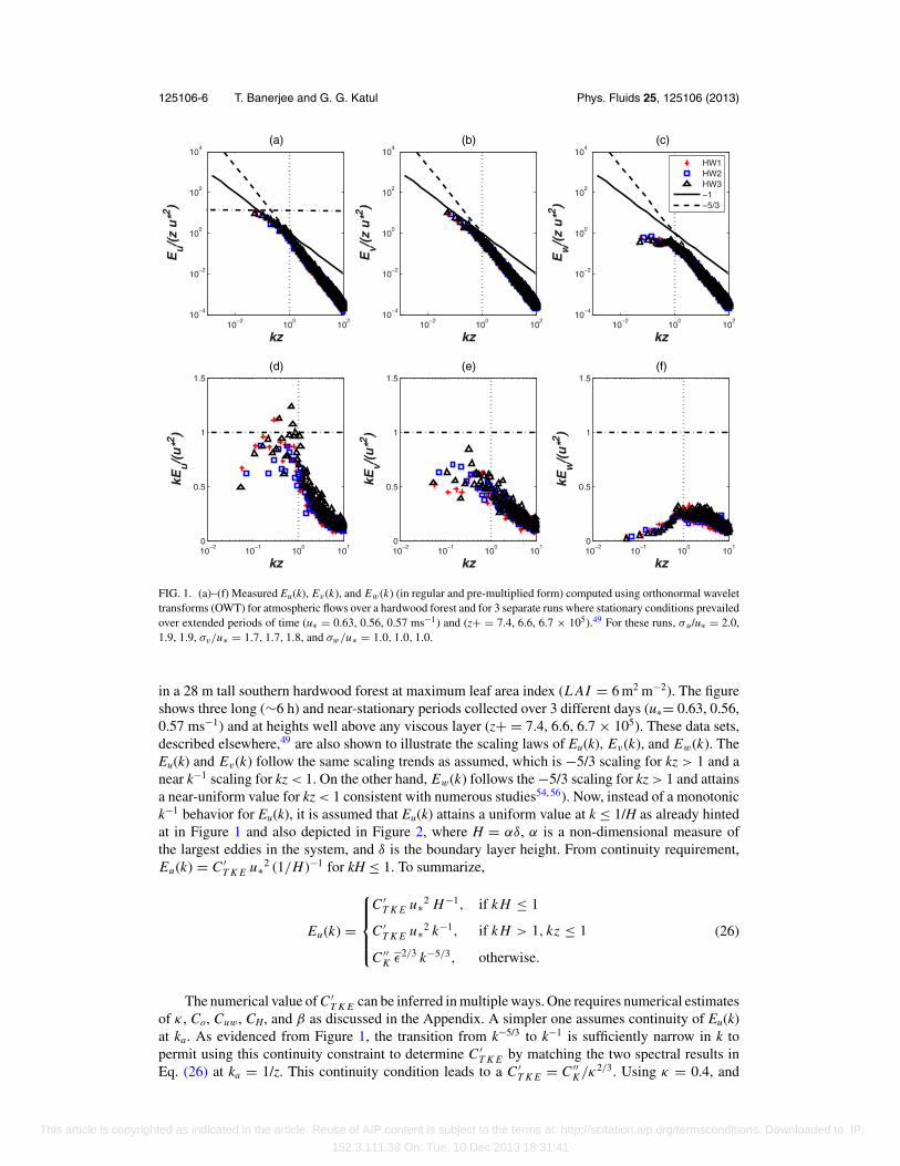
FIG. 1. (a)–(f) Measured Eu(k), Ev(k), and Ew(k) (in regular and pre-multiplied form) computed using orthonormal wavelettransforms (OWT) for atmospheric flows over a hardwood forest and for 3 separate runs where stationary conditions prevailedover extended periods of time (u∗ = 0.63, 0.56, 0.57 ms−1) and (z+ = 7.4, 6.6, 6.7 × 105).49 For these runs, σ u/u∗ = 2.0,1.9, 1.9, σv/u∗ = 1.7, 1.7, 1.8, and σw/u∗ = 1.0, 1.0, 1.0.

in a 28 m tall southern hardwood forest at maximum leaf area index (L AI = 6 m2 m−2). The figureshows three long (∼6 h) and near-stationary periods collected over 3 different days (u∗= 0.63, 0.56,0.57 ms−1) and at heights well above any viscous layer (z+ = 7.4, 6.6, 6.7 × 105). These data sets,described elsewhere,49 are also shown to illustrate the scaling laws of Eu(k), Ev(k), and Ew(k). TheEu(k) and Ev(k) follow the same scaling trends as assumed, which is −5/3 scaling for kz > 1 and anear k−1 scaling for kz < 1. On the other hand, Ew(k) follows the −5/3 scaling for kz > 1 and attainsa near-uniform value for kz < 1 consistent with numerous studies54, 56). Now, instead of a monotonick−1 behavior for Eu(k), it is assumed that Eu(k) attains a uniform value at k ≤ 1/H as already hintedat in Figure 1 and also depicted in Figure 2, where H = αδ, α is a non-dimensional measure ofthe largest eddies in the system, and δ is the boundary layer height. From continuity requirement,Eu(k) = C ′

T K E u∗2 (1/H )−1 for kH ≤ 1. To summarize,

Eu(k) =

⎧⎪⎪⎨⎪⎪⎩

C ′T K E u∗2 H−1, if k H ≤ 1

C ′T K E u∗2 k−1, if k H > 1, kz ≤ 1

C ′′K ε2/3 k−5/3, otherwise.

(26)

The numerical value of C ′T K E can be inferred in multiple ways. One requires numerical estimates

of κ , Co, Cuw, CH, and β as discussed in the Appendix. A simpler one assumes continuity of Eu(k)at ka. As evidenced from Figure 1, the transition from k−5/3 to k−1 is sufficiently narrow in k topermit using this continuity constraint to determine C ′

T K E by matching the two spectral results inEq. (26) at ka = 1/z. This continuity condition leads to a C ′

T K E = C ′′K /κ2/3. Using κ = 0.4, and

This article is copyrighted as indicated in the article. Reuse of AIP content is subject to the terms at: http://scitation.aip.org/termsconditions. Downloaded to IP:

152.3.111.38 On: Tue, 10 Dec 2013 18:31:41

125106-7 T. Banerjee and G. G. Katul Phys. Fluids 25, 125106 (2013)

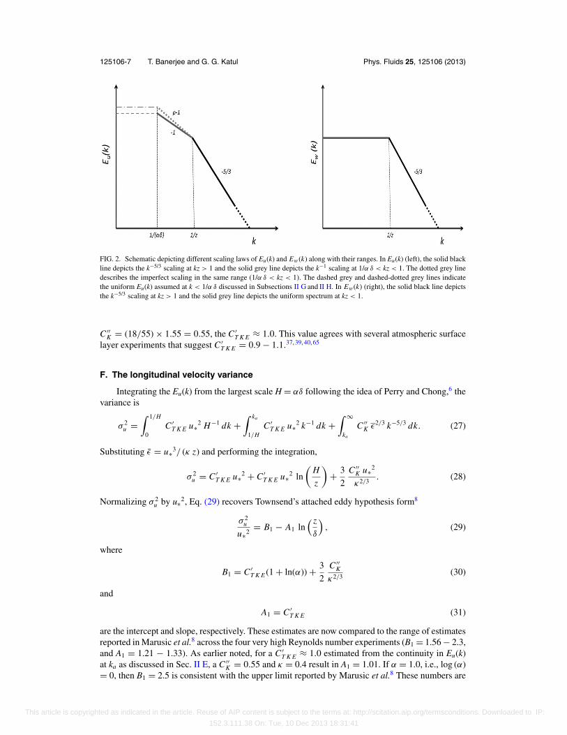
FIG. 2. Schematic depicting different scaling laws of Eu(k) and Ew(k) along with their ranges. In Eu(k) (left), the solid blackline depicts the k−5/3 scaling at kz > 1 and the solid grey line depicts the k−1 scaling at 1/α δ < kz < 1. The dotted grey linedescribes the imperfect scaling in the same range (1/α δ < kz < 1). The dashed grey and dashed-dotted grey lines indicatethe uniform Eu(k) assumed at k < 1/α δ discussed in Subsections II G and II H. In Ew(k) (right), the solid black line depictsthe k−5/3 scaling at kz > 1 and the solid grey line depicts the uniform spectrum at kz < 1.

C ′′K = (18/55) × 1.55 = 0.55, the C ′

T K E ≈ 1.0. This value agrees with several atmospheric surfacelayer experiments that suggest C ′

T K E = 0.9 − 1.1.37, 39, 40, 65

F. The longitudinal velocity variance

Integrating the Eu(k) from the largest scale H = αδ following the idea of Perry and Chong,6 thevariance is

σ 2u =

∫ 1/H

0C ′

T K E u∗2 H−1 dk +∫ ka

1/HC ′

T K E u∗2 k−1 dk +∫ ∞

ka

C ′′K ε2/3 k−5/3 dk. (27)

Substituting ε = u∗3/ (κ z) and performing the integration,

σ 2u = C ′

T K E u∗2 + C ′T K E u∗2 ln

(H

z

)+ 3

2

C ′′K u∗2

κ2/3. (28)

Normalizing σ 2u by u∗2, Eq. (29) recovers Townsend’s attached eddy hypothesis form8

σ 2u

u∗2= B1 − A1 ln

( z

δ

), (29)

where

B1 = C ′T K E (1 + ln(α)) + 3

2

C ′′K

κ2/3(30)

and

A1 = C ′T K E (31)

are the intercept and slope, respectively. These estimates are now compared to the range of estimatesreported in Marusic et al.8 across the four very high Reynolds number experiments (B1 = 1.56 − 2.3,and A1 = 1.21 − 1.33). As earlier noted, for a C ′

T K E ≈ 1.0 estimated from the continuity in Eu(k)at ka as discussed in Sec. II E, a C ′′

K = 0.55 and κ = 0.4 result in A1 = 1.01. If α = 1.0, i.e., log (α)= 0, then B1 = 2.5 is consistent with the upper limit reported by Marusic et al.8 These numbers are

This article is copyrighted as indicated in the article. Reuse of AIP content is subject to the terms at: http://scitation.aip.org/termsconditions. Downloaded to IP:

152.3.111.38 On: Tue, 10 Dec 2013 18:31:41

125106-8 T. Banerjee and G. G. Katul Phys. Fluids 25, 125106 (2013)

TABLE I. The values of α (95% confidence level with intervals) computed using nonlinear least squares method along withthe coefficient of determination (R2) and the root mean square error RMSE using Eq. (29). The spectral shape associatedwith the model is depicted in Figure 2 using the dotted blue, solid blue, and solid and dotted black lines.

Experiment α 95% confidence interval R2 RMSE Fitted equation

Melbourne 1.56 (1.41, 1.72) 0.96 0.16 Eq. (29)Superpipe 0.76 (0.68, 0.83) 0.96 0.19 Eq. (29)LCC 1.36 (1.24, 1.48) 0.96 0.19 Eq. (29)SLTEST 1.58 (0.98, 2.19) 0.87 0.37 Eq. (29)

also close to the empirical estimates of A1 = 1.03 and B1 = 2.39 provided in Smits, McKeon, andMarusic.14 The other estimates of B1 and A1 using the alternate estimate of C ′

T K E is discussed in theAppendix. Also, it is interesting to note that for the three runs collected above the hardwood forestreported in Figure 1, σ u/u∗ = 2.0, 1.9, 1.9. For a typical daytime neutral atmospheric boundary δ

= 1000 m, a measurement height of about 40 m, a zero-plane displacement height of 2/3 canopyheight, A1 = C ′′

K /κ2/3 = 1.01 and a B1 = (1 + 3/2)A1, result in σ u/u∗ = 2.4, reasonably close to thefield measurements here (∼2.0).

G. Effect of very large scale motion (VLSM)

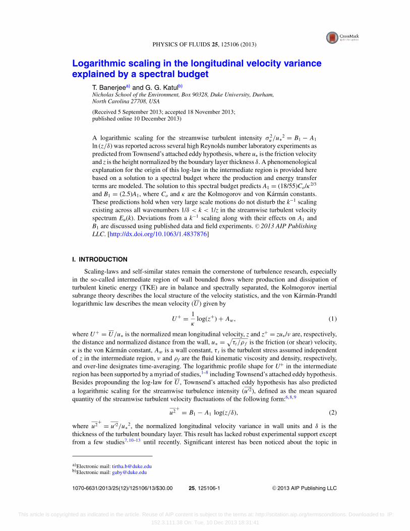
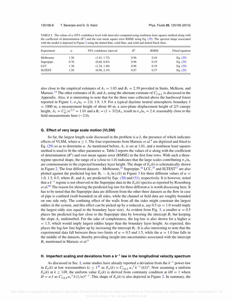
So far, the largest length scale discussed in the problem is α δ, the presence of which indicateseffects of VLSM, where α ≥ 1. The four experiments from Marusic et al.8 are digitized and fitted toEq. (29) so as to determine α. As mentioned before, A1 is set at 1.01, and a nonlinear least squaresmethod is used to fit the other parameter α. Table I reports the values of α along with the coefficientof determination (R2) and root mean square error (RMSE) in the first four rows. With such a three-regime spectral shape, the range of α (close to 1.0) indicates that the large scales contributing σ u/u∗are commensurate to the expected boundary layer height. The shape of Eu(k) is schematically shownin Figure 2. The four different datasets – Melbourne,18 Superpipe,16 LCC,19 and SLTEST17 are alsoplotted against the predicted log-law B1 − A1 ln (z/δ) in Figure 3 for three different values of α =1.0, 1.5, 0.5, where B1 and A1 are predicted by Eqs. (30) and (31), respectively. It is however, notedthat a k−1 regime is not observed in the Superpipe data in the Eu(k) spectra as reported by Rosenberget al.66 The reason for showing the predicted log-law for three different α is worth discussing here. Ithas to be noted that the Superpipe data are different from the other three datasets as the flow in caseof pipe is confined (wall-bounded) in all sides, while the channel or field data are roughly boundedon one side only. The confining effect of the walls from all the sides might constrain the largesteddies in the system, and this effect can be picked up by a reduced α, say 0.5 (α = 1.0 would implythe largest eddy size equal to the boundary layer size). As evident from Fig. 3, a smaller α = 0.5places the predicted log-law close to the Superpipe data by lowering the intercept B1 but keepingthe slope A1 undisturbed. For the sake of completeness, the log-law is also shown for a higher α

= 1.5, which would imply largest eddies larger than the boundary layer height. As expected, thisplaces the log-law line higher up by increasing the intercept B1. It is also interesting to note that theexperimental data fall between these two limits of α = 0.5 and 1.5, while the α = 1.0 line falls inthe middle of the datasets, thereby providing insight into uncertainties associated with the interceptB1 mentioned in Marusic et al.8

H. Imperfect scaling and deviations from a k−1 law in the longitudinal velocity spectrum

As discussed in Sec. I, some studies have already reported a deviation from the k−1 power-lawin Eu(k) at low wavenumbers kz ≤ 149 as Eu(k) = C ′

T K E u∗2 k−1 (kδ)p. Now assuming a uniformEu(k) at k ≤ 1/H, the uniform value Eu(k) is derived from continuity condition at kH = 1 whereH = α δ as C ′

T K E u∗2 δ (1/α)p−1. This shape of Eu(k) is also depicted in Figure 2. In summary, the

This article is copyrighted as indicated in the article. Reuse of AIP content is subject to the terms at: http://scitation.aip.org/termsconditions. Downloaded to IP:

152.3.111.38 On: Tue, 10 Dec 2013 18:31:41

125106-9 T. Banerjee and G. G. Katul Phys. Fluids 25, 125106 (2013)

10−2

10−1

3

3.5

4

4.5

5

5.5

6

6.5

7

7.5

8

σ u2 /u*2

z/δ

SLTEST dataSuperpipe dataLCC dataMelbourne dataModel (α=1.0)Model (α=1.5)Model (α=0.5)

FIG. 3. Four different datasets presented by Marusic et al.,8 namely, the Melbourne, Superpipe, LCC, and SLTEST data,against the predicted log-law B1 − A1 ln(z/δ) for three different values of α = 1.0, 1.5, 0.5, where B1 and A1 are predictedby Eqs. (30) and (31), respectively.

imperfect scaling can be written as

Eu(k) =

⎧⎪⎪⎨⎪⎪⎩

C ′T K E u∗2 δ (1/α)p−1 if k H ≤ 1

C ′T K E u∗2 k−1 (kδ)p , if k H > 1, kz ≤ 1

C ′′K ε2/3 k−5/3. otherwise

, (32)

where p can be any real number, and δ is the height of the boundary layer as before. As before,continuity requirement at kz = 1 leads to C ′

T K E = (C ′′K /κ2/3) (z/δ)p. Performing the integration as

in Eq. (27) and using this value of C ′T K E ,

σ 2u =

∫ 1/H

0C ′

T K E u∗2 δ (1/α)p−1 dk +∫ k1

1/HC ′

T K E u∗2 δ p k p−1 dk +∫ ∞

k1=1/zC ′′

K ε (k1)2/3 k−5/3 dk.

(33)Simplifying, and normalizing by u∗2,

σ 2u

u∗2=

(C ′′

K

κ2/3

) ( z

δ

)pα−p + 3

2

C ′′K

κ2/3+ 1

p

C ′′K

κ2/3

(1 −

( z

δ

)p(

1

α

)p). (34)

The datasets are fitted using a nonlinear least squares method with Eq. (34) and values of p andα are shown in the first four rows of Table II.

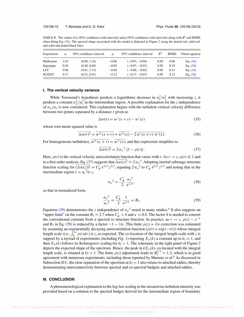
From Table II, a power law deviated from −1 by p may be a plausible description to the Eu(k)scaling at kz ≤ 1 for the data reported in Marusic et al.8 Also, a constant Eu(k) at kH ≤ 1 seems to bea plausible representation if a near unity in α is used as an evaluation metric. However, it should be

emphasized that a finite p leads to power-law dependence of u2+

on z/δ instead of logarithmic. Theranges of values of p is to be noted in Table II, indicating roughly a power-law of k−1.08 instead of ak−1 scaling. The pre-multiplied spectra presented in Rosenberg et al.66 (arguing against a k−1 scaling)and Nickels et al.48 (supporting a limited k−1 scaling), when digitized, also indicate a deviation inthe pre-multiplied spectral ordinate of about 0.3, which strongly suggests the presence of a powerlaw k−1.08 instead of a k−1 scaling.

This article is copyrighted as indicated in the article. Reuse of AIP content is subject to the terms at: http://scitation.aip.org/termsconditions. Downloaded to IP:

152.3.111.38 On: Tue, 10 Dec 2013 18:31:41

125106-10 T. Banerjee and G. G. Katul Phys. Fluids 25, 125106 (2013)

TABLE II. The values of α (95% confidence with intervals) and p (95% confidence with intervals) along with R2 and RMSEwhen fitting Eq. (34). The spectral shape associated with the model is depicted in Figure 2 using the dotted red, solid red,and solid and dotted black lines.

Experiment α 95% confidence interval p 95% confidence interval R2 RMSE Fitted equation

Melbourne 1.03 (0.90, 1.16) −0.06 (−0.07, −0.04) 0.99 0.06 Eq. (34)Superpipe 0.54 (0.48, 0.60) −0.05 (−0.07, −0.03) 0.99 0.10 Eq. (34)LCC 0.96 (0.81, 1.12) −0.04 (−0.06, −0.02) 0.98 0.14 Eq. (34)SLTEST 0.71 (0.51, 0.91) −0.12 (−0.17, −0.07) 0.99 0.12 Eq. (34)

I. The vertical velocity variance

While Townsend’s hypothesis predicts a logarithmic decrease in σ 2u /u2

∗ with increasing z, itpredicts a constant σ 2

w/u2∗ in the intermediate region. A possible explanation for the z independence

of σw/u∗ is now considered. This explanation begins with the turbulent vertical velocity differencebetween two points separated by a distance r given as

�w(r ) = w′ (x + r ) − w′ (x) (35)

whose root-mean squared value is

�w(r )2 = w′2 (x + r ) + w′2 (x) − 2 w′ (x + r ) w′ (x). (36)

For homogeneous turbulence, w′2 (x + r ) = w′2 (x), and this expression simplifies to

�w(r )2 = 2 σw2 [1 − ρ(r )] . (37)

Here, ρ(r) is the vertical velocity autocorrelation function that varies with r. As r → z, ρ(r) 1 andin a first order analysis, Eq. (37) suggests that �w(z)2 ≈ 2 σw

2. Adopting inertial subrange structurefunction scaling for (�w(z))2 = C ′

K ε2/3 z2/3, equating 2 σw2 to C ′

K ε2/3 z2/3 and noting that in theintermediate region ε = u∗3/κ z,

σw2 = C ′

K

2

u∗2

κ2/3, (38)

so that in normalized form,

σw2

u∗2= C ′

K

2

1

κ2/3= B3. (39)

Equation (39) demonstrates the z independence of σw2 noted in many studies.6 It also suggests an

“upper-limit” on the constant B3 ≈ 2.7 when C ′K × 4 and κ = 0.4. The factor 4 is needed to convert

the conventional constant from a spectral to structure function. In practice, as r → z, ρ(z) ∼ e−1

and B3 in Eq. (39) is reduced by a factor ∼1 − 1/e. This finite ρ(z) = 1/e correction was estimatedby assuming an exponentially decaying autocorrelation function (ρ(r) = exp (−r/z)) whose integrallength scale (i.e.,

∫ ∞0 ρ(r )dr ) is z, as expected. The co-location of the integral length scale with z is

support by a myriad of experiments (including Fig. 1) reporting Ew(k) a constant up to kz = 1, andthen Ew(k) follows its Kolmogorov scaling for kz > 1. The schematic in the right panel of Figure 2depicts the expected shape of the spectrum. Hence, the peak in k Ew(k), co-located with the integrallength scale, is situated at kz = 1. The finite ρ(z) adjustment leads to B1/2

3 = 1.3, which is in goodagreement with numerous experiments, including those reported by Marusic et al.8 As discussed inSubsection II C, the clear separation of the spectrum at kz = 1 also relates to attached eddies, therebydemonstrating interconnectivity between spectral and co-spectral budgets and attached eddies.

III. CONCLUSION

A phenomenological explanation to the log-law scaling in the streamwise turbulent intensity wasprovided based on a solution to the spectral budget derived for the intermediate region of boundary

This article is copyrighted as indicated in the article. Reuse of AIP content is subject to the terms at: http://scitation.aip.org/termsconditions. Downloaded to IP:

152.3.111.38 On: Tue, 10 Dec 2013 18:31:41

125106-11 T. Banerjee and G. G. Katul Phys. Fluids 25, 125106 (2013)

layers. Linking of a co-spectral budget to the spectral budget by means of a production term whosemain source is Ew(k)56 is noted. Dividing the Ew(k) spectrum in two different zones at ka = z−1

reveals underlying connections to Townsend’s attached eddy hypothesis. The breakpoint at ka =z−1 is clearly observed in many Ew(k) spectra within the intermediate region, dividing the eddiesinto attached manifesting a k−5/3 scaling at kz ≥ 1 and detached eddies often indicated by a flatspectrum at kz ≤ 1, though this low-wavenumber portion is not used here beyond its consequence onEtke(k) ≈ Eu(k) for this range of wavenumbers. Thus, the co-spectral budget, the spectral budget, andTownsend’s attached eddy hypothesis encoded in the shape of Ew(k) are all brought under a commonframework to predict the logarithmic scaling in the streamwise turbulent intensity. Because inertialsubrange scaling for the u′ spectrum was assumed for k > 1/z, the coefficients associated with thelogarithmic scaling in the streamwise turbulent intensity were then linked to the Kolmogorov andvon Karman constants. When the k−1 scaling was extended to all k < 1/z, the predicted constantsdescribing the log-law scaling differed by some 20% from measured values reported using laboratoryexperiments at high Reynolds numbers. Deviation from the k−1 scaling in the u′ spectrum for kz <

1 have also been discussed, along with the effects of VLSM on these constants. It was demonstratedvia calculations here that these spectral exponent deviations can be commensurate to k−1.06. If so,then σ 2

u /u∗2 exhibits power-law instead of logarithmic scaling in z/δ, though the difference betweenthe two in terms of statistical fitting to the data may be too small to discern.

ACKNOWLEDGMENTS

T.B. and G.K. acknowledge support from the National Science Foundation (NSF) (NSF-AGS-1102227), the United States Department of Agriculture (2011-67003-30222), the (U.S.) Departmentof Energy (DOE) through the office of Biological and Environmental Research (BER) TerrestrialEcosystem Science (TES) Program (DE-SC0006967), and the Binational Agricultural Research andDevelopment (BARD) Fund (IS-4374-11C). G.K. thanks C. Meneveau for the helpful discussionsduring their joint visit at Ecole Polytechnique Federale de Lausanne (EPFL) in 2013.

APPENDIX: AN ALTERNATE ESTIMATE OF C ′TKE

An alternate estimate of C ′T K E is now discussed. To evaluate this estimate based on Cb, it is

necessary to provide numerical values for C ′′K , Cuw, and CH in the context of a certain interpretation

of k. For three-dimensional isotropic turbulence, it can be shown that CH = (8/9)C−3/2o as discussed

elsewhere.67 Interestingly, this isotropic estimate of CH can also be recovered from the spectralbudget here when production and viscous terms are absent so that the energy transfer F(ka) at anyarbitrary ka is entirely balanced by ε resulting in

ε = [νt (ka)]

[∫ ka

02Co(ε)2/3 p−5/3dp

]=

[3CH C1/2

o ε1/3

4k4/3a

] [3

4k4/3

a 2Co(ε)2/3

]. (A1)

Noting that ε and ka cancel out in Eq. (A1), and upon re-arranging, the CH = (8/9)C−3/2o is

recovered even when interpreting k as a one-dimensional cut in the longitudinal direction. With thisformulation for CH, CT K E = 2Cb = (Co)(3/2)(κ4/3 − (3/4)Cuw)/κ2. Using κ = 0.4, Cuw = 0.15 asdiscussed before in the derivation of Fwu(k), and Co = 1.55 × [(18 + 24 + 24)/2]/55 = 0.93 resultin CTKE = 1.5. Estimating C ′

T K E requires a further discussion about the proportionality constant β

because C ′T K E = β CT K E . In the inertial subrange and at kz > 1, β = (18/55)CK/(33/55)CK ≈ (18/33)

≈ 0.5. However, in the integrated spectrum, there are contributions from all wavenumbers and β ≈ 1.0based on e = (1/2)(σ 2

u + σ 2v + σ 2

w) with σ 2w + σ 2

v ≈ σ 2u . It may be surmised that β varies between 0.5

and 1.0. With β = 1.0, C ′T K E = 1.5, thereby estimating B1 = C ′

T K E (1 + ln(α)) + (3/2) C ′′K /κ2/3 =

3.0 and A1 = C ′T K E = 1.5, which are higher than the numbers reported by Marusic et al.8 With a

β of 0.8 (between 0.5 and 1.0), it results in B1 = 2.6 and A1 = 1.1, close to the range provided byMarusic et al.8 (B1 = 1.56 − 2.3 and A1 = 1.21 − 1.33).

This article is copyrighted as indicated in the article. Reuse of AIP content is subject to the terms at: http://scitation.aip.org/termsconditions. Downloaded to IP:

152.3.111.38 On: Tue, 10 Dec 2013 18:31:41

125106-12 T. Banerjee and G. G. Katul Phys. Fluids 25, 125106 (2013)

1 L. Prandtl, Z. Angew. Math. Mech. 5, 136 (1925).2 T. Von Karman, Nachr. Ges. Wiss. Goettingen, Math.-Phys. Kl. 1930, 58 (1930).3 C. B. Millikan, in Proceedings of the 5th International Congress of Applied Mechanics (Wiley, New York, 1938),

pp. 386–392.4 J. Rotta, Prog. Aerosp. Sci. 2, 1 (1962).5 A. A. Townsend, The Structure of Turbulent Shear Flow (Cambridge University Press, 1976).6 A. Perry and M. Chong, J. Fluid Mech. 119, 173 (1982).7 A. Perry and J. Li, J. Fluid Mech. 218, 405 (1990).8 I. Marusic, J. P. Monty, M. Hultmark, and A. J. Smits, J. Fluid Mech. 716, R3 (2013).9 C. Meneveau and I. Marusic, J. Fluid Mech. 719, R1 (2013).

10 A. Perry and C. Abell, J. Fluid Mech. 79, 785 (1977).11 A. Perry, S. Henbest, and M. Chong, J. Fluid Mech. 165, 163 (1986).12 A. Perry and I. Marusic, J. Fluid Mech. 298, 361 (1995).13 J. Jimenez and S. Hoyas, J. Fluid Mech. 611, 215 (2008).14 A. J. Smits, B. J. McKeon, and I. Marusic, Annu. Rev. Fluid Mech. 43, 353 (2011).15 A. J. Smits and I. Marusic, Phys. Today 66(9), 25 (2013).16 M. Hultmark, M. Vallikivi, S. Bailey, and A. Smits, Phys. Rev. Lett. 108, 094501 (2012).17 N. Hutchins, K. Chauhan, I. Marusic, J. Monty, and J. Klewicki, Boundary-Layer Meteorol. 145, 273 (2012).18 V. Kulandaivelu, “Evolution of zero pressure gradient turbulent boundary layers from different initial conditions,” Ph.D.

thesis, Department of Mechanical Engineering, The University of Melbourne, 2012.19 E. S. Winkel, J. M. Cutbirth, S. L. Ceccio, M. Perlin, and D. R. Dowling, Exp. Therm. Fluid Sci. 40, 140 (2012).20 C. Tchen, J. Res. Natl. Bur. Stand. 50, 51 (1953).21 C.-M. Tchen, Phys. Rev. 93, 4 (1954).22 P. Klebanoff, “Characteristics of turbulence in a boundary layer with zero pressure gradient,” Report No. 1247 (National

Advisory Committee for Aeronautics, 1954), p. 19.23 J. Hinze, Turbulence: An Introduction to its Mechanisms and Theory (McGraw-Hill, New York, USA, 1959), p. 586.24 S. Pond, S. Smith, P. Hamblin, and R. Burling, J. Atmos. Sci. 23, 376 (1966).25 K. Bremhorst and K. Bullock, Int. J. Heat Mass Transfer 13, 1313 (1970).26 S. Panchev, Random Functions and Turbulence (Pergamon Press, Oxford, 1971), p. 443.27 K. Bremhorst and T. Walker, J. Fluid Mech. 61, 173 (1973).28 A. Perry and C. Abell, J. Fluid Mech. 67, 257 (1975).29 B. Korotkov, Izv. Akad. Nauk SSSR, Ser. Mekh. Zhidk. I. Gaza 6, 35 (1976).30 K. Bullock, R. Cooper, and F. Abernathy, J. Fluid Mech. 88, 585 (1978).31 I. Hunt and P. Joubert, J. Fluid Mech. 91, 633 (1979).32 B. Kader and A. Yaglom, in Nonlinear and Turbulent Processes in Physics, edited by R. Z. Sagdeyev (Hardwood, 1984),

Vol. 2, p. 829.33 A. Perry, K. Lim, and S. Henbest, J. Fluid Mech. 177, 437 (1987).34 A. Turan, R. Azad, and S. Kassab, Phys. Fluids 30, 3463 (1987).35 L. Erm, A. Smits, and P. Joubert, “Low Reynolds number turbulent boundary layers on a smooth flat surface in a zero

pressure gradient,” Turbulent Shear Flows 5 (Springer-Verlag, Berlin, 1987), pp. 186–196.36 L. Erm and P. Joubert, J. Fluid Mech. 230, 1 (1991).37 B. Kader and A. Yaglom, “Spectra and correlation functions of surface layer atmospheric turbulence in unstable thermal

stratification,” in Turbulence and Coherent Structures (Kluwer Academic Press, Dordrecht, 1991), pp. 387–412.38 A. Yaglom, Phys. Fluids 6, 962 (1994).39 G. G. Katul, J. D. Albertson, C.-I. Hsieh, P. S. Conklin, J. T. Sigmon, M. B. Parlange, and K. R. Knoerr, J. Atmos. Sci. 53,

2512 (1996).40 G. Katul and C.-R. Chu, Boundary-Layer Meteorol. 86, 279 (1998).41 J. Jimenez, Physica A 263, 252 (1999).42 V. Nikora, Phys. Rev. Lett. 83, 734 (1999).43 W. George, and M. Tutkun, in Progress in Wall Turbulence: Understanding and Modeling, edited by M. Stanislas,

J. Jimenez, and I. Marusic (Springer, Netherlands, 2011), Vol. 14, pp. 183–190.44 A. N. Kolmogorov, Dokl. Akad. Nauk SSSR 30, 299–303 (1941).45 J. Kaimal, J. Atmos. Sci. 35, 18 (1978).46 R. Antonia and M. Raupach, Boundary-Layer Meteorol. 65, 289 (1993).47 J. Morrison, W. Jiang, B. McKeon, and A. Smits, Phys. Rev. Lett. 88, 214501 (2002).48 T. Nickels, I. Marusic, S. Hafez, and M. Chong, Phys. Rev. Lett. 95, 074501 (2005).49 G. G. Katul, A. Porporato, and V. Nikora, Phys. Rev. E 86, 066311 (2012).50 W. Heisenberg, Proc. R. Soc. London, Ser. A 195, 402 (1948).51 G. J. Kunkel and I. Marusic, J. Fluid Mech. 548, 375 (2006).52 I. Marusic, B. McKeon, P. Monkewitz, H. Nagib, A. Smits, and K. Sreenivasan, Phys. Fluids 22, 065103 (2010).53 R. B. Stull, An Introduction to Boundary Layer Meteorology (Kluwer Academic Publishers, 1988), Vol. 666.54 S. Pope, Turbulence Flows (Cambridge University Press, Cambridge, UK, 2000), p. 779.55 G. I. Taylor, Proc. R. Soc. London, Ser. A 164, 476 (1938).56 G. G. Katul, A. Porporato, C. Manes, and C. Meneveau, Phys. Fluids 25, 091702 (2013).57 B. Kader and A. Yaglom, J. Fluid Mech. 212, 637 (1990).58 M. Raupach, J. Fluid Mech. 108, 363 (1981).59 K. Choi and J. Lumley, J. Fluid Mech. 436, 59 (2001).60 W. Bos, H. Touil, L. Shao, and J.-P. Bertoglio, Phys. Fluids 16, 3818 (2004).

This article is copyrighted as indicated in the article. Reuse of AIP content is subject to the terms at: http://scitation.aip.org/termsconditions. Downloaded to IP:

152.3.111.38 On: Tue, 10 Dec 2013 18:31:41

125106-13 T. Banerjee and G. G. Katul Phys. Fluids 25, 125106 (2013)

61 J. Lumley, Phys. Fluids 10, 855 (1967).62 S. Saddoughi and S. Veeravalli, J. Fluid Mech. 268, 333 (1994).63 D. Cava and G. Katul, Boundary-Layer Meteorol. 145, 351 (2012).64 T. Ishihara, K. Yoshida, and Y. Kaneda, Phys. Rev. Lett. 88, 154501 (2002).65 G. G. Katul, C. R. Chu, M. B. Parlange, J. D. Albertson, and T. A. Ortenburger, J. Geophys. Res., [Atmos.] 100, 14243,

doi:10.1029/94JD02616 (1995).66 B. Rosenberg, M. Hultmark, M. Vallikivi, S. Bailey, and A. Smits, J. Fluid Mech. 731, 46 (2013).67 U. Schumann, Beitr. Phys. Atmos. 67, 141 (1994).

This article is copyrighted as indicated in the article. Reuse of AIP content is subject to the terms at: http://scitation.aip.org/termsconditions. Downloaded to IP:

152.3.111.38 On: Tue, 10 Dec 2013 18:31:41