Locating Binding Constraints in LP Problems · Linear Programming, Simplex, Binding Constraints, Weighted Average 1. Introduction It is well-known, that in large linear programming

American Journal of Operations Research, 2019, 9, 59-78 http://www.scirp.org/journal/ajor

ISSN Online: 2160-8849 ISSN Print: 2160-8830

DOI: 10.4236/ajor.2019.92004 Mar. 7, 2019 59 American Journal of Operations Research

Locating Binding Constraints in LP Problems

Eirini I. Nikolopoulou, George E. Manoussakis, George S. Androulakis

Department of Business Administration, University of Patras, Patras, Greece

Abstract In this work, a new method is presented for determining the binding con-straints of a general linear maximization problem. The new method uses only objective function values at points which are determined by simple vector operations, so the computational cost is inferior to the corresponding cost of matrix manipulation and/or inversion. This method uses a recently proposed notion for addressing such problems: the average of each constraint. The identification of binding constraints decreases the complexity and the dimen-sion of the problem resulting to a significant decrease of the computational cost comparing to Simplex-like methods. The new method is highly useful when dealing with very large linear programming (LP) problems, where only a relatively small percentage of constraints are binding at the optimal solu-tion, as in many transportation, management and economic problems, since it reduces the size of the problem. The method has been implemented and tested in a large number of LP problems. In LP problems without superfluous constraints, the algorithm was 100% successful in identifying binding con-straints, while in a set of large scale LP tested problems that included super-fluous constraints, the power of the algorithm considered as statistical tool of binding constraints identification, was up to 90.4%.

Keywords Linear Programming, Simplex, Binding Constraints, Weighted Average

1. Introduction

It is well-known, that in large linear programming (LP) problems there is a sig-nificant number of redundant constraints and variables. Simplex method [1] [2] [3] [4] had reigned supreme as the preferred method for solving such linear programs for many decades. This method starts from the worst possible vertex (the origin) and converges to the best solution of the LP problem at a finite number of iterations after having created a set of basic feasible solutions (vertic-

How to cite this paper: Nikolopoulou, E.I., Manoussakis, G.E. and Androulakis, G.S. (2019) Locating Binding Constraints in LP Problems. American Journal of Operations Research, 9, 59-78. https://doi.org/10.4236/ajor.2019.92004 Received: January 21, 2019 Accepted: March 4, 2019 Published: March 7, 2019 Copyright © 2019 by author(s) and Scientific Research Publishing Inc. This work is licensed under the Creative Commons Attribution International License (CC BY 4.0). http://creativecommons.org/licenses/by/4.0/

Open Access

http://www.scirp.org/journal/ajor

https://doi.org/10.4236/ajor.2019.92004

http://www.scirp.org


http://creativecommons.org/licenses/by/4.0/

E. I. Nikolopoulou et al.

DOI: 10.4236/ajor.2019.92004 60 American Journal of Operations Research

es). Nevertheless, Simplex method is expensive and demands too much compu-tational time in large scale problems. If the number of constraints is too large, then so is the number of vertices, and therefore there is a large probability that Simplex will need a big number of iterations. Since real life LP problems are ac-tually large scaled, the development of techniques for reducing considerably the dimension of the problem, became an inevitable need. This problem reduction, among others, results to less computational time and effort.

In this direction, many researchers including Andersen and Andersen [5], Ba-linsky [6], Boot [7], Brearly et al. [8], Boneh et al. [9], Caron et al. [10], Ioslovich [11], Gal [12], Gutman and Isolovich [13], Mattheis [14], Nikolopoulou et al. [15], Stojkovic and Staminirovic [16], Paulraj et al. [17] [18] and Telgen [19] have proposed several algorithms to identify redundant constraints in order to reduce the dimension of the initial large scale LP problem. Brearly et al. [8] pro-posed a method to identify redundant constraints using the upper and lower bounds of the variables. Telgen [19] proposed a deterministic method to identify redundant constraints using minimum-ratio criteria as in Simplex method hav-ing similar complexity with Simplex. Stojković and Stanimirović method [16] identifies redundant constraints applying the maximum and minimum prin-ciple. Paulraj et al. [17] proposed a heuristic method to identify redundant con-straints based on the intercept matrix of constraints of the LP problem. Ilya Ios-lovich method [11] identifies the redundant constraints in large scale linear problems with box constraints and positive or zero coefficients. The Gaussian elimination or QR factorization has been proposed but causes many and serious difficulties including significant rise of the dimension of the problem and re-quirement of floating point operations [16]. Unfortunately, all proposed algo-rithms for the elimination of the excessive constraints do not guarantee com-plete elimination.

In this work, a new method is presented for determining the binding con-straints of a general linear maximization problem. The method deals with the general n-dimensional linear maximization problem with more constraints than decision variables in a standard form, i.e. with functional constraints of the type lesser-than-or-equal and no negativity constraints. It is based on the notion of a kind of weighted average of the decision variables associated with each con-straint boundary. Actually, this average is one coordinate of the point at which the bisector line of the first angle of the axis (the line whose points have equal coordinates) intersects the hyperplane defined by the constraint boundary equa-tion.

The proposed method is always applicable to linear programming problems which are defined with no excessive constraints. Sometimes, it is applicable even in the cases when there are superfluous constraints in the problems. It uses only objective function values at points which are determined by simple vector opera-tions, so the computational cost is inferior to the corresponding cost of matrix manipulation and/or inversion. The new method has been implemented and tested and results are presented.




This paper is organized as follows: in Section 2, there is a discussion on the average of the optimum based on the weighted average of each constraint and in Section 3, the new method is presented using a geometrical approach. The pro-posed algorithm is presented in Section 4 and the computational cost is pre-sented in Section 5. In Section 6, the results of the algorithm tested in random LP problems are presented. Finally, in Section 7, we conclude with some remarks on the proposed algorithm and possible extensions.

2. A Discussion about the Average of the Optimum 2.1. Mathematical Framework

Many real-life problems consist of maximizing or minimizing a certain quantity subject to several constraints. Specifically, linear programming (LP) involves op-timization (maximization or minimization) of a linear objective function on several decision variables subject to linear constraints.

In mathematical notation, a normal form of an LP multidimensional problem can be expressed as follows:

( ) Tmaxsubject to

0

z X C XAX bX

=

≤≥

(1.1)

where: X is the n-dimensional vector of decision variables,

ij m naA

× = , [ ]i m

b b= , j mC c =

with ija ∈ , jc ∈ and 0jb > for 1,2, ,i m= and 1,2, ,j n= are the coefficients of the LP-problem and ( ) Tz X C X= is the objective function.

The feasible region of this problem is the set of all possible feasible points, i.e. points in ℝn that satisfy all constraints in (1.1). The feasible region in n dimen-sions is a hyper-polyhedron. More specifically, in two dimensions, the bounda-ries are formed by line segments, and the feasible region is a polygon. An optim-al solution is the feasible solution with the largest objective function value (for a maximization problem). In this paper we consider linear problems for which the feasible region forms a convex nonempty set.

The extreme points or vertices of a feasible region are those boundary points that are intersections of the straight-line boundary segments of the region. If a linear programming problem has a solution, it must occur at a vertex of the set of feasible solutions. If the problem has more than one solution, then at least one of them must occur at an extreme point. In either case, the value of the optimal value of the objective function is unique.

Definition 1: A constraint is called “binding” or “active” if it is satisfied as an equality at the optimal solution, i.e. if the optimal solution lies on the surface having the corresponding equation (plane of the constraint). Otherwise the con-straint is called “redundant”.

Definition 2: If the plane of a redundant constraint does not contain feasible




points (it is beyond the feasible region) then the constraint is called superfluous. Both types of redundant constraints are included in problem formulation

since it is not known a priori that they are superfluous or nonbinding. Definition 3: The zero-level planes together with the planes of all the con-

straints except the superfluous define the boundary of the feasible region. We refer to these constraints as “functional”.

Any redundant constraint may be dropped from the problem, and the infor-mation lost by dropping this constraint (the amount of excess associated with the constraint) can be easily computed once the optimum solution has been found.

The existence of superfluous constraints does not alter the optimum solutions, but may require many additional iterations to be taken, and increases the com-putational cost.

Most of the methods proposed to date for identification of redundant and nonbinding constraints are not warranted in practice because of the excessive computations required to implement them.

Unfortunately, there is no easy method of assuring a convex solution path, except in two-dimensional problems nor is there any way of preventing degene-racy [20].

We make the assumption that the feasible region is convex and it is formed by the whole set of constraints so that each constraint refers to a side of the polygon feasible region. So our problem should not contain superfluous constraints.

2.2. A Notion about the Weighted Average

Consider the LP problem (1.1). In this problem, constraints could be binding and redundant, nevertheless, as it was mentioned before, in the considered problem there are not superfluous constraints included. For the completeness of the present work, some necessary hypotheses are made and definitions are given.

Let ( )1 2, , , nX x x x∗ ∗ ∗ ∗= be the optimal solution of the problem (1.1). Since the binding constraints hold equality in the system of inequalities in problem (1.1), X ∗ is a solution of each binding constraint of the problem (1.1).

Definition 4: Consider the LP problem (1.1). Let

1 1 1

n n ni ij ij ij i ijj j j

a x a b aλ= = =

= =∑ ∑ ∑

be the weighted average of the random constraint i. Then, the𝑛𝑛-dimensional vector ( )* , , ,i i i iλ λ λ λ= is a solution of this con-

straint. The𝑛𝑛-dimensional vector *iλ , 1,2, ,i m= is defined by the weighted

average of the i-constraints. The coordinates of *iλ , 1,2, ,i m= of the prob-

lem (1.1) are the points of the bisector line of the first angle of the axis(the hyperplane whose points have equal coordinates) intersects the hyperplane de-fined by the constraint boundary equation.

In most cases, i sλ , 1,2, ,i m= are different from each other but it can




happen that two or more i sλ are the same although the corresponding con-straints are totally different.

The 𝑚𝑚-dimensional vector that represents the weighted average for each con-straint is given as:

( )1 2, , , mλ λ λ λ= . (1.2)

Τhen, the weighted average of the 𝑘𝑘-th binding constraint of the LP problem (1.1) is given as:

1n

k k kjjb aλ=

= ∑ . (1.3)

Since the constraint k is binding, defines the optimal solution and then the corresponding *

kλ can be considered as an estimator of the optimal solution of the LP problem (1.1) [21]. This estimation may differ from the actual solution.

As it was presented in this section, i sλ , 1,2, ,i m= have been considered as solutions of potential equality constraints, so the main reflection is how to identify necessary constraints using these *

i sλ , 1,2, ,i m= . For this purpose, *i sλ , 1,2, ,i m= are used as a probabilistic order of the constraint impor-

tance of the LP problem (1.1). In this direction, the solutions *

i sλ , 1,2, ,i m= are sorted. Point( )min min min, , ,M λ λ λ where { }min :min 1,2, ,i i mλ λ= = is a point of the

constraint having this specific solution: ( )*min min min min, , ,λ λ λ λ= .

As the feasible area is defined by the planes of the convex polyhedron, point M is a feasible point. Point M is actually the only point at which the bisector plane of the first angle of the axes intersects the boundary of the feasible region, i.e. the other *

i sλ , apart from *minλ lie beyond the feasible area of the problem.

Moreover, point M lies on the face “opposite the origin”. The proposed method starts by setting the value of the variables equal to

minλ , so the starting point is the point M, which is a point of the feasible area, lies on a constraint and on the bisector plane. Moreover, point M is set across the origin, which is the Simplex starting point.

Simplex method starts by setting the value of the variables equal to zero and then proceeds to find the optimum value of the objective function. The starting point is the origin. Hence, by setting the variables to zero as the starting point that is the origin. This starting point is relatively far from the optimum.

Our method starts from the point M, which is in general a point across the origin. Point M is a boundary point of the feasible area, and its coordinates are the weighted average of a constraint of the problem, therefore point M lies on this constraint. In case the constraint is binding, the constraint defines the op-timal solution and the coordinates of point M are considered as an estimator of the optimal solution of the LP problem. Since the main goal of optimization al-gorithms in LP problems is to achieve the optimum, point M is certainly a better estimator of the optimum than the origin.

The algorithm checks for binding constraints considering one decision varia-ble each time. Using the weighted average and the intercepts of the constraints




with the zero level hyperplane of the variable under consideration, the algorithm moves from a constraint to an adjacent one until it locates a binding constraint.

3. The New Method: A Geometrical Proof of Convergence

The 2-dimensional case For a LP problem with two decision variables the feasible region is, as men-

tioned, a convex polygon with 2m + edges in general (including the two axes). The maximum of the objective function is located on a vertex of this polygon, so it is defined by two binding constraints (one or two of them can be a no negativ-ity constraint in the case that the solution is degenerated). Our scope is to locate these two binding constraints.

Each axis defines two opposite directions. If we slide the objective function line along one of them then the objective function value increases, while along its opposite it decreases. To recognize which is which it suffices to compare the objective function value on two points. These two points can be chosen to be-long on the edge defined by a constraint. Specifically, we choose the intersection of the constraint with the bisector and the intersection of the constraint with the other axis. Thus we can easily locate the increasing direction for any axis.

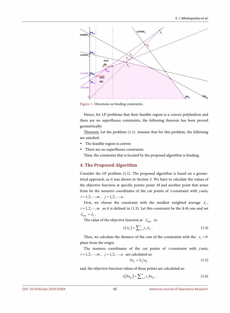
Consider a random LP problem with two decision variables and five con-straints. Figure 1 illustrates this procedure. Let us consider that we have two ad-jacent edges (constraints). If the increasing directions on these constraints are opposite, then, it is clear, that the optimal vertex is the intersection of these edges (see Figure 1). That means that these two constraints are the binding ones.

Given a constraint, to locate his adjacent to a specific direction, let’s say in re-spect to 1x it suffices to check the distance of the intersection of this constraint with the 2x -axis from the origin, due to the convexity of the feasible region. Specifically, if the increasing direction is the one decreasing the 1x value, then the adjacent to a constraint j is the one whose intersection with the 2x -axis has the next smaller distance from the origin. The result for the opposite direction is obvious.

We conclude that the location of the two binding constraints is the result of the directional search in respect to only one of the two variables.

The n-dimensional case The above results can be easily generalized for the n-dimensional problem,

since any plenary projection of the feasible region is a convex polygon. The adjacent constraint is defined with the aid of the distance of the cuts of

the constraints with the 0ix = plane from the origin, where i is the search di-rection. The only issue is that there can be several adjacent constraints to a given constraint, so there is no guaranty that an adjacent constraint is not overlooked. Also since the adjacent constraints lie in several directions, one must repeat the procedure for more than one variable. During the search for binding constraints along each direction, an opposition of increasing directions defines one binding constraint.




Figure 1. Directions on binding constraints.

Hence, for LP problems that their feasible region is a convex polyhedron and there are no superfluous constraints, the following theorem has been proved geometrically:

Theorem: Let the problem (1.1). Assume that for this problem, the following are satisfied: The feasible region is convex There are no superfluous constraints

Then, the constraint that is located by the proposed algorithm is binding.

4. The Proposed Algorithm

Consider the LP problem (1.1). The proposed algorithm is based on a geome-trical approach, as it was shown in Section 3. We have to calculate the values of the objective function at specific points: point M and another point that arises from be the nonzero coordinates of the cut points of i-constraint with j-axis,

1, 2, ,i m= , 1,2, ,j n= . First, we choose the constraint with the smallest weighted average iλ ,1, 2, ,i m= as it is defined in (1.3). Let this constraint be the k-th one and set

min kλ λ= . The value of the objective function at minλ is:

( ) 1n

k j kjz cλ λ=

= ∑ . (1.4)

Then, we calculate the distance of the cuts of the constraints with the 0ix = plane from the origin.

The nonzero coordinates of the cut points of i-constraint with j-axis, 1, 2, ,i m= , 1,2, ,j n= are calculated as:

ij i ijbx b a= (1.5)

and, the objective function values of these points are calculated as:

( ) 1n

kj j kjjz bx c bx=

= ∑ . (1.6)




Start the searching in respect to jx , 1,2, ,j n= . During the search for binding constraints, an opposition of increasing directions defines one binding constraint.

The increasing direction of the objective function is considered as the index

0r which is defined in the following equation:

( ) ( )( ) ( )0 kj k kj kr z bx z bxλ λ= − − . (1.7)

If 0 0r > then the increasing direction is the positive one, i.e. the direction that jx is augmenting. Otherwise, the direction is the one that

jx is decreasing. Then find the adjacent constraint in the chosen direction that is described below:

The distance of the cut of the constraint with the plane 0ix = , i j≠ from the origin is given as:

21,

nij i ikk k jdx b a

= ≠= ∑ . (1.8)

To continue, we move to the constraint following the chosen direction re-garding the distance ijdx , for 1,2, ,j m= .

The adjacent constraint in the chosen direction is the one having the next bigger (respectively smaller) distance in case the direction is increasing (respec-tively decreasing). If there is no bigger (respectively smaller) distance in this di-rection, then this constraint is binding, otherwise compute the 0r index for the next constraint.

If the 0r index for the next constraint has different sign from the previous index, then the increasing direction has changed and the last constraint is bind-ing. In case there is no constraint that has a different direction, then the corres-ponding variable is considered as zero and this constraint is binding. Repeat the process for the next decision variable 1jx + .

After finding n-binding constraints or after having exhausted the n-variables, stop the procedure.

The steps of the proposed algorithm are described below:

The proposed algorithm algorithm bi.co.fi input: The number of decision variables (n), the number of constraints (m),

the coefficient matrix of the problem (A), the vector of the right-hand side coef-ficients (b), the vector of the objective coefficients (C).

output: The vector of binding constraints ( )1 2, , , nv v v= v Compute iλ , ( ) 1, 2, ,i i m∀ = using Equation (1.3) Se min kλ λ= , where k is the constraint with minλ If there are more than two constraints having the same minλ , then choose randomly one of them. Compute ( )kz λ using Equation (1.4) If 0ija = then set 10000000ijbx = else compute ijbx , ( ) ( ), 1, 2, , , 1, 2, ,i j i m j n∀ = = using Equation (1.5) end if




Compute ( )kjz bx , ( )1,2, ,j j n∀ = using Equation (1.6) if

21, 0n

ikk k j a= ≠=∑

then set 10000000ijdx = else compute ijdx , ( ) ( ), 1, 2, , , 1, 2, ,i j i m j n∀ = = using Equation (1.8) end if for 1,2, ,j n= do

_ jdx Order Order dx←

place ← the order of _dx Order in position k If ( ) ( ) 0kj kz bx z λ− = then print 0 If 0kj kbx λ− = then print 0 Compute 0r in position k using Equation (1.7) if sign of 0 1r = then sequence (start = place, end = m, 1) else sequence(start = place, end = 1, −1) end if for t = start, , end

0jv ←

new place ← t + sign of 0r if new place = 0 or new place = 1m + then

jv ← the constraint in new place break end if set 0rpev r= Compute 0r in new place gin = 0rpev r∗ if gin < 0 then

jv ← the constraint in new place break end if end second for end first for

5. Computational Cost

Consider a LP problem of n variables and m constraints, with m and m n> , and large (so quantities such as m or n are negligible in comparison to m2 or mn). The array needed to solve this problem using Simplex is ( ) ( )1 1m n+ × + . Working on the proposed algorithm, only an array of n n× is needed to solve the same problem, so the dimension reduction is obvious. The number of itera-tions using the Simplex method is on average ( ) 2n m+ [22].

The number of iterations of the proposed algorithm is 𝑛𝑛 at the most, which is the number of variables. Sometimes, the number of needed iterations is even less (for example in 2-variable problems).

The number of multiplications (or divisions) required in each iteration of the




Simplex algorithm is ( )( )1 1m n+ + , ignoring the cost of the ratio test, while the number of additions (or subtractions) is roughly the same [23]. On average, the total number of operations using Simplex algorithm is ( )( )( )1 1m n n m+ + + .

To find the total number of operations of the proposed algorithm the compu-tational cost of 0r , ιλ , ijbx and ijdx , 1,2, ,i m= , 1,2, ,j n= must be added. The total evaluation cost of the multiplications is on average

2 4 2 2mn mn n m+ + + + and the total evaluation cost of the additions is on av-erage ( )1mn n − . Finally, the total number of operations using the proposed al-gorithm is 22 3 2 2mn mn n m+ + + + .

It is obvious that for m n> not only the number of iterations of the new method is less than the corresponding number of Simplex but also the total computational cost is significant inferior. If one adds the cost of solving an 𝑛𝑛𝑛𝑛𝑛𝑛 system of equation for the binding constraints found ( 32 3n operations) to compute the optimal solution (so that the results of the two methods are com-parable) the total computational cost remains significantly inferior (gain of or-der at least 2n ). The gain on computational cost increases as m becomes much bigger than n.

6. Numerical Results

In this section, the numerical results of the proposed algorithm are presented. In the first part, a LP problem is illustrated. In second part the comparative results of the approach of the proposed algorithm and Simplex method for identifying binding constraints in indicative LP problems are presented. Finally, the algo-rithm was considered as a statistical tool for correctly identifying binding con-straints in random linear programming problems and the results of this statistic-al approach are presented in the third part of the section. The proposed algo-rithm was implemented in R language [24] in more than 3000 LP problems. In LP problems where there were no superfluous constraints and the feasible area was a convex dome-shaped region, the proposed algorithm was 100% accurate in correctly identifying binding constraints.

6.1. Illustration of a LP Problem

The following numerical example serves to illustrate the proposed algorithm. Consider the LP maximization problem (1.9) with three decision variables and four constraints:

( ) 1 2 3

1 2 3

1 2 3

1 2 3

1 2 3

20 10 153 2 5 55

m

2

axsubject t

263 30

o

5 2 4 570

x x xx x xx x x

x x xx x

z X

xX

+ +

+ + ≤

+ + ≤

+ + ≤

+ + ≤

≥

=

where X is the 3-dimensional vector of decision variables




1

2

3

3 2 5 5520

2 1 1 26, , , 10

1 1 3 3015

5 2 4 57

xX x A b C

x

= = = =

and ( ) Tz X C X= is the objective function. In this problem, according to Simplex method the third constraint is redun-

dant, so the first, the second and the fourth constraints are binding. It also known that the third constraint is not superfluous.

According to (1.2), ( )5.5,6.5,6,5.18λΤ = . The smallest iλ , 1,2,3,4i = is

4 5.18λ = and it is referring to the fourth constraint. Thus, min 4λ λ= .

The matrices of

4 3ijbx bx×

= and 4 3

ijdx dx×

=

are given below, however, not all of these elements of these matrices are needed to be calculated in advance.

Each element is calculated whenever it is needed

18.3 27.5 1113 26 2630 30 10

11.4 28.5 14.25

bx

=

,

10.213 9.432 15.25410.213 11.627 11.6279.486 9.486 21.213

12.745 8.902 10.584

dx

=

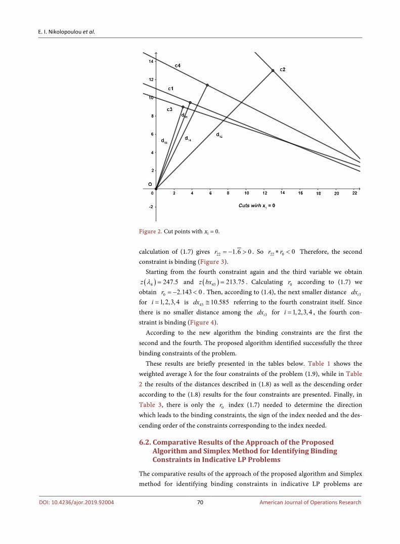
We start from the fourth constraint and the first variable, according to (1.4) and (1.6) respectively and we find ( )4 233.18z λ = and ( )41 288z bx = . Then according to (1.7) we obtain 0 0.83 0r = − < . Then, according to (1.6), the next smaller distance is 1idx for 1,2,3,4i = is 11 10.213dx ≅ referring to the first constraint. For the first constraint, ( )11 366.6z bx = and 11 9.2857 0r = > . Since

11 0 0r r∗ < the first constraint is binding. This process is illustrated in Figure 2 below.

Starting again from the fourth constraint and the second variable, we obtain( )4 233.18z λ = and ( )42 285z bx = . In this case, according to (1.7)

0 2.2 0r = > . The next bigger distance 2idx for 1,2,3,4i = is 12 9.432dx ≅ referring to the first constraint. For the first constraint, the calculation of (1.6) is( )12 275z bx = and the calculation of (1.7) is 12 1.25 0r = > . Then, we obtain

12 0 0r r∗ > . So we must continue the search. The next bigger distance is

32 9.487dx ≅ referring to the third constraint. We set 12 0r r= . For the third constraint, ( )32 300z bx = and 32 1.25 0r = > . Applying the re-

sults, we obtain 32 0 0r r∗ > . The next bigger distance 2idx for 01, 2,3, 4i = is

22 11.627dx ≅ , referring to the second constraint. We set 32r r= . For the second constraint, the calculation of (1.6) is ( )22 260z bx = and the




Figure 2. Cut points with x1 = 0.

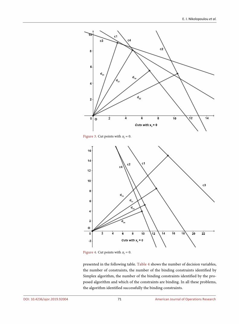
calculation of (1.7) gives 22 1.6 0r = − > . So 22 0 0r r∗ < Therefore, the second constraint is binding (Figure 3).

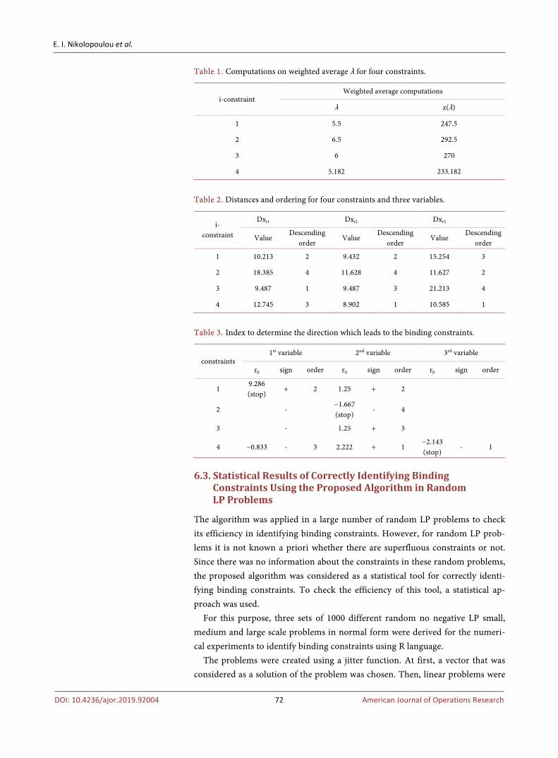
Starting from the fourth constraint again and the third variable we obtain( )4 247.5z λ = and ( )43 213.75z bx = . Calculating 0r according to (1.7) we

obtain 0 2.143 0r = − < . Then, according to (1.4), the next smaller distance 3idx for 1,2,3,4i = is 43 10.585dx ≅ referring to the fourth constraint itself. Since there is no smaller distance among the 3idx for 1,2,3,4i = , the fourth con-straint is binding (Figure 4).

According to the new algorithm the binding constraints are the first the second and the fourth. The proposed algorithm identified successfully the three binding constraints of the problem.

These results are briefly presented in the tables below. Table 1 shows the weighted average λ for the four constraints of the problem (1.9), while in Table 2 the results of the distances described in (1.8) as well as the descending order according to the (1.8) results for the four constraints are presented. Finally, in Table 3, there is only the 0r index (1.7) needed to determine the direction which leads to the binding constraints, the sign of the index needed and the des-cending order of the constraints corresponding to the index needed.

6.2. Comparative Results of the Approach of the Proposed Algorithm and Simplex Method for Identifying Binding Constraints in Indicative LP Problems

The comparative results of the approach of the proposed algorithm and Simplex method for identifying binding constraints in indicative LP problems are






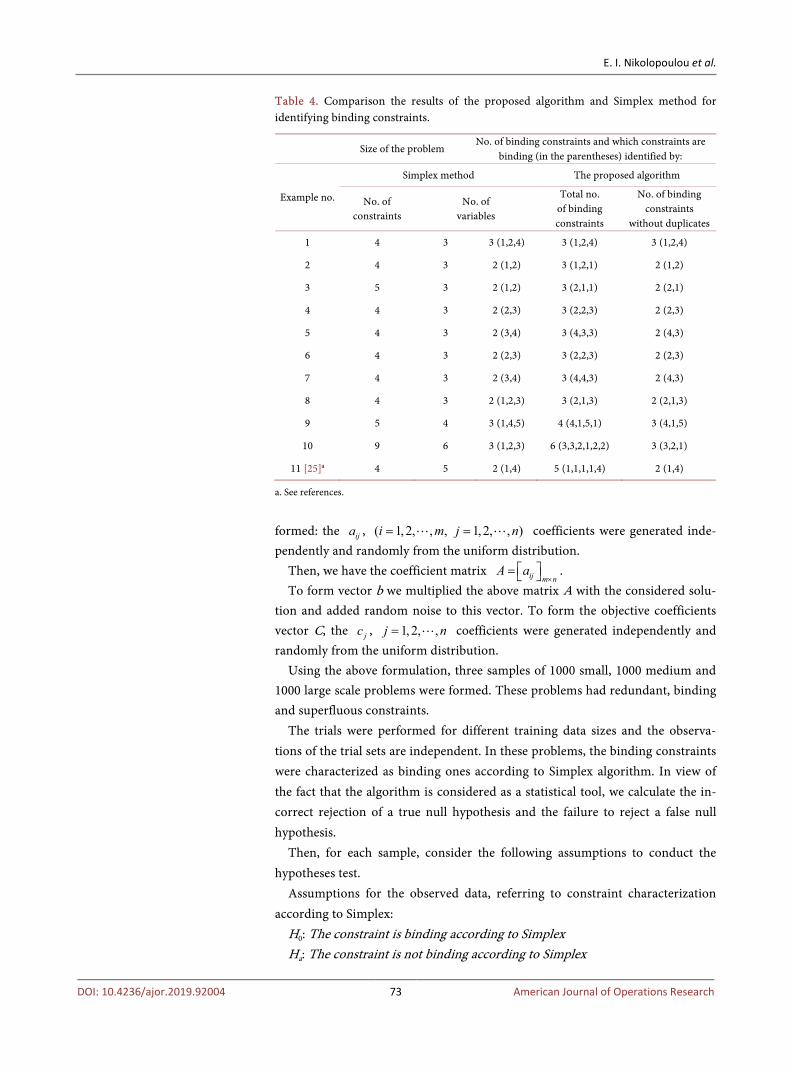
presented in the following table. Table 4 shows the number of decision variables, the number of constraints, the number of the binding constraints identified by Simplex algorithm, the number of the binding constraints identified by the pro-posed algorithm and which of the constraints are binding. In all these problems, the algorithm identified successfully the binding constraints.




Table 1. Computations on weighted average λ for four constraints.

i-constraint Weighted average computations

λ z(λ)

1 5.5 247.5

2 6.5 292.5

3 6 270

4 5.182 233.182

Table 2. Distances and ordering for four constraints and three variables.

i- constraint

Dxi1 Dxi2 Dxi3

Value Descending

order Value

Descending order

Value Descending

order

1 10.213 2 9.432 2 15.254 3

2 18.385 4 11.628 4 11.627 2

3 9.487 1 9.487 3 21.213 4

4 12.745 3 8.902 1 10.585 1

Table 3. Index to determine the direction which leads to the binding constraints.

constraints 1st variable 2nd variable 3rd variable

r0 sign order r0 sign order r0 sign order

1 9.286 (stop)

+ 2 1.25 + 2

2 - −1.667 (stop)

- 4

3 - 1.25 + 3

4 −0.833 - 3 2.222 + 1 −2.143 (stop)

- 1

6.3. Statistical Results of Correctly Identifying Binding Constraints Using the Proposed Algorithm in Random LP Problems

The algorithm was applied in a large number of random LP problems to check its efficiency in identifying binding constraints. However, for random LP prob-lems it is not known a priori whether there are superfluous constraints or not. Since there was no information about the constraints in these random problems, the proposed algorithm was considered as a statistical tool for correctly identi-fying binding constraints. To check the efficiency of this tool, a statistical ap-proach was used.

For this purpose, three sets of 1000 different random no negative LP small, medium and large scale problems in normal form were derived for the numeri-cal experiments to identify binding constraints using R language.

The problems were created using a jitter function. At first, a vector that was considered as a solution of the problem was chosen. Then, linear problems were




Table 4. Comparison the results of the proposed algorithm and Simplex method for identifying binding constraints.

Size of the problem No. of binding constraints and which constraints are

binding (in the parentheses) identified by:

Example no.

Simplex method The proposed algorithm

No. of constraints

No. of variables

Total no. of binding constraints

No. of binding constraints

without duplicates

1 4 3 3 (1,2,4) 3 (1,2,4) 3 (1,2,4)

2 4 3 2 (1,2) 3 (1,2,1) 2 (1,2)

3 5 3 2 (1,2) 3 (2,1,1) 2 (2,1)

4 4 3 2 (2,3) 3 (2,2,3) 2 (2,3)

5 4 3 2 (3,4) 3 (4,3,3) 2 (4,3)

6 4 3 2 (2,3) 3 (2,2,3) 2 (2,3)

7 4 3 2 (3,4) 3 (4,4,3) 2 (4,3)

8 4 3 2 (1,2,3) 3 (2,1,3) 2 (2,1,3)

9 5 4 3 (1,4,5) 4 (4,1,5,1) 3 (4,1,5)

10 9 6 3 (1,2,3) 6 (3,3,2,1,2,2) 3 (3,2,1)

11 [25]a 4 5 2 (1,4) 5 (1,1,1,1,4) 2 (1,4)

a. See references.

formed: the ija , ( 1, 2, , , 1, 2, , )i m j n= = coefficients were generated inde-pendently and randomly from the uniform distribution.

Then, we have the coefficient matrix m nijaA×

= . To form vector b we multiplied the above matrix A with the considered solu-

tion and added random noise to this vector. To form the objective coefficients vector C, the jc , 1,2, ,j n= coefficients were generated independently and randomly from the uniform distribution.

Using the above formulation, three samples of 1000 small, 1000 medium and 1000 large scale problems were formed. These problems had redundant, binding and superfluous constraints.

The trials were performed for different training data sizes and the observa-tions of the trial sets are independent. In these problems, the binding constraints were characterized as binding ones according to Simplex algorithm. In view of the fact that the algorithm is considered as a statistical tool, we calculate the in-correct rejection of a true null hypothesis and the failure to reject a false null hypothesis.

Then, for each sample, consider the following assumptions to conduct the hypotheses test.

Assumptions for the observed data, referring to constraint characterization according to Simplex:

H0: The constraint is binding according to Simplex Ha: The constraint is not binding according to Simplex




And Assumptions for the predicted data, referring to constraint characterization

according to the proposed algorithm: H0: The constraint is considered as binding according to the proposed algo-

rithm Ha: The constraint cannot be considered as binding according to the proposed

algorithm Let P1: The probability that there are binding constraints (according to Simplex

method) among the constraints that characterized as binding by the proposed algorithm.

P2: The probability a constraint can’t be characterized as binding according to the proposed algorithm even though the constraint is binding according to Simplex method.

P3: The probability a constraint that is not binding according to Simplex me-thod is characterized as binding according to the proposed algorithm.

P4: The probability a constraint that can’t be characterized as binding by the proposed algorithm isn’t binding according to Simplex method.

P5: The probability that binding constraints according to Simplex method are included among the constraints that are characterized as binding by the pro-posed algorithm.

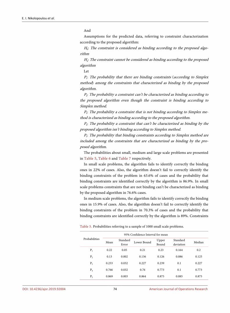
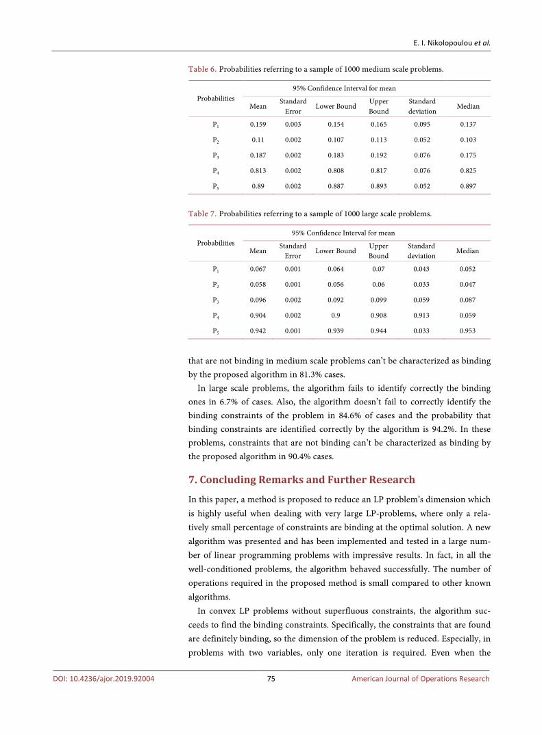
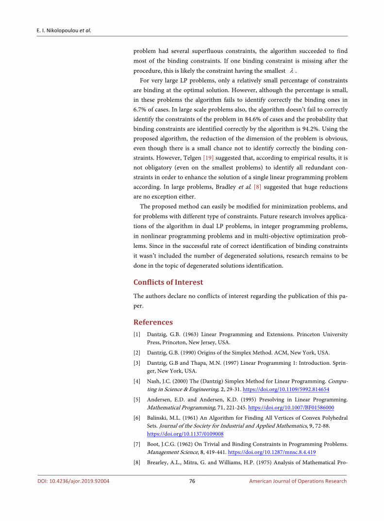
The probabilities about small, medium and large scale problems are presented in Table 5, Table 6 and Table 7 respectively.

In small scale problems, the algorithm fails to identify correctly the binding ones in 22% of cases. Also, the algorithm doesn’t fail to correctly identify the binding constraints of the problem in 63.6% of cases and the probability that binding constraints are identified correctly by the algorithm is 86.9%. In small scale problems constraints that are not binding can’t be characterized as binding by the proposed algorithm in 76.6% cases.

In medium scale problems, the algorithm fails to identify correctly the binding ones in 15.9% of cases. Also, the algorithm doesn’t fail to correctly identify the binding constraints of the problem in 70.3% of cases and the probability that binding constraints are identified correctly by the algorithm is 89%. Constraints Table 5. Probabilities referring to a sample of 1000 small scale problems.

Probabilities 95% Confidence Interval for mean

Mean Standard

Error Lower Bound

Upper Bound

Standard deviation

Median

P1 0.22 0.05 0.21 0.23 0.164 0.2

P2 0.13 0.002 0.136 0.126 0.086 0.125

P3 0.233 0.032 0.227 0.239 0.1 0.227

P4 0.766 0.032 0.76 0.773 0.1 0.773

P5 0.869 0.003 0.864 0.875 0.085 0.875




Table 6. Probabilities referring to a sample of 1000 medium scale problems.


Mean Standard

Error Lower Bound

Upper Bound

Standard deviation

Median

P1 0.159 0.003 0.154 0.165 0.095 0.137

P2 0.11 0.002 0.107 0.113 0.052 0.103

P3 0.187 0.002 0.183 0.192 0.076 0.175

P4 0.813 0.002 0.808 0.817 0.076 0.825

P5 0.89 0.002 0.887 0.893 0.052 0.897

Table 7. Probabilities referring to a sample of 1000 large scale problems.


Mean Standard

Error Lower Bound

Upper Bound

Standard deviation

Median

P1 0.067 0.001 0.064 0.07 0.043 0.052

P2 0.058 0.001 0.056 0.06 0.033 0.047

P3 0.096 0.002 0.092 0.099 0.059 0.087

P4 0.904 0.002 0.9 0.908 0.913 0.059

P5 0.942 0.001 0.939 0.944 0.033 0.953

that are not binding in medium scale problems can’t be characterized as binding by the proposed algorithm in 81.3% cases.

In large scale problems, the algorithm fails to identify correctly the binding ones in 6.7% of cases. Also, the algorithm doesn’t fail to correctly identify the binding constraints of the problem in 84.6% of cases and the probability that binding constraints are identified correctly by the algorithm is 94.2%. In these problems, constraints that are not binding can’t be characterized as binding by the proposed algorithm in 90.4% cases.

7. Concluding Remarks and Further Research

In this paper, a method is proposed to reduce an LP problem’s dimension which is highly useful when dealing with very large LP-problems, where only a rela-tively small percentage of constraints are binding at the optimal solution. A new algorithm was presented and has been implemented and tested in a large num-ber of linear programming problems with impressive results. In fact, in all the well-conditioned problems, the algorithm behaved successfully. The number of operations required in the proposed method is small compared to other known algorithms.

In convex LP problems without superfluous constraints, the algorithm suc-ceeds to find the binding constraints. Specifically, the constraints that are found are definitely binding, so the dimension of the problem is reduced. Especially, in problems with two variables, only one iteration is required. Even when the




problem had several superfluous constraints, the algorithm succeeded to find most of the binding constraints. If one binding constraint is missing after the procedure, this is likely the constraint having the smallest λ .

For very large LP problems, only a relatively small percentage of constraints are binding at the optimal solution. However, although the percentage is small, in these problems the algorithm fails to identify correctly the binding ones in 6.7% of cases. In large scale problems also, the algorithm doesn’t fail to correctly identify the constraints of the problem in 84.6% of cases and the probability that binding constraints are identified correctly by the algorithm is 94.2%. Using the proposed algorithm, the reduction of the dimension of the problem is obvious, even though there is a small chance not to identify correctly the binding con-straints. However, Telgen [19] suggested that, according to empirical results, it is not obligatory (even on the smallest problems) to identify all redundant con-straints in order to enhance the solution of a single linear programming problem according. In large problems, Bradley et al. [8] suggested that huge reductions are no exception either.

The proposed method can easily be modified for minimization problems, and for problems with different type of constraints. Future research involves applica-tions of the algorithm in dual LP problems, in integer programming problems, in nonlinear programming problems and in multi-objective optimization prob-lems. Since in the successful rate of correct identification of binding constraints it wasn’t included the number of degenerated solutions, research remains to be done in the topic of degenerated solutions identification.

Conflicts of Interest

The authors declare no conflicts of interest regarding the publication of this pa-per.

References [1] Dantzig, G.B. (1963) Linear Programming and Extensions. Princeton University

Press, Princeton, New Jersey, USA.

[2] Dantzig, G.B. (1990) Origins of the Simplex Method. ACM, New York, USA.

[3] Dantzig, G.B and Thapa, M.N. (1997) Linear Programming 1: Introduction. Sprin-ger, New York, USA.

[4] Nash, J.C. (2000) The (Dantzig) Simplex Method for Linear Programming. Compu-ting in Science & Engineering, 2, 29-31. https://doi.org/10.1109/5992.814654

[5] Andersen, E.D. and Andersen, K.D. (1995) Presolving in Linear Programming. Mathematical Programming, 71, 221-245. https://doi.org/10.1007/BF01586000

[6] Balinski, M.L. (1961) An Algorithm for Finding All Vertices of Convex Polyhedral Sets. Journal of the Society for Industrial and Applied Mathematics, 9, 72-88. https://doi.org/10.1137/0109008

[7] Boot, J.C.G. (1962) On Trivial and Binding Constraints in Programming Problems. Management Science, 8, 419-441. https://doi.org/10.1287/mnsc.8.4.419

[8] Brearley, A.L., Mitra, G. and Williams, H.P. (1975) Analysis of Mathematical Pro-


https://doi.org/10.1109/5992.814654

https://doi.org/10.1007/BF01586000

https://doi.org/10.1137/0109008

https://doi.org/10.1287/mnsc.8.4.419



gramming Problems Prior to Applying the Simplex Algorithm. Mathematical Pro-gramming, 8, 54-83. https://doi.org/10.1007/BF01580428

[9] Boneh, A., Boneh, S. and Caron, R.J. (1993) Constraint Classification in Mathemat-ical Programming. Mathematical Programming, 61, 61-73. https://doi.org/10.1007/BF01582139

[10] Caron, R.J., McDonald, J.F. and Ponic, C.M. (1989) A Degenerate Extreme Point Strategy for the Classification of Linear Constraints as Redundant or Necessary. Journal of Optimization Theory and Applications, 62, 225-237. https://doi.org/10.1007/BF00941055

[11] Ioslovich, I. (2001) Robust Reduction of a Class of Large-Scale Linear Programs. SIAM Journal of Optimization, 12, 262-282. https://doi.org/10.1137/S1052623497325454

[12] Gal, T. (1992) Weakly Redundant Constraints and Their Impact on Post Optimal Analysis. European Journal of Operational Research, 60, 315-326. https://doi.org/10.1016/0377-2217(92)90083-L

[13] Gutman, P.O. and Isolovich, I. (2007) Robust Redundancy Determination and Evaluation of the Dual Variables of Linear Programming Problems in the Presence of Uncertainty, on the Generalized Wolf Problem: Preprocessing of Nonnegative Large Scale Linear Programming Problems with Group Constraints. Tech-nion-Israel Institute of Technology, 68, 1401-1409.

[14] Mattheis, T.H. (1973) An Algorithm for Determining Irrelevant Constraints and All Vertices in Systems of Linear Inequalities. Operations Research, 21, 247-260. https://doi.org/10.1287/opre.21.1.247

[15] Nikolopoulou, E., Nikas, I. and Androulakis, G. (2017) Redundant Constraints Identification in Linear Programming Using Statistics on Constraints. Proceedings of the 6th International Symposium & 28th National Conference on Operational Research/OR in the Digital Era—ICT Challenges, Thessaloniki, 8-10 June 2017, 196-201.

[16] Stojković, N.V. and Stanimirović, P.S. (2001) Two Direct Methods in Linear Pro-gramming. European Journal of Operational Research, 131, 417-439. https://doi.org/10.1016/S0377-2217(00)00083-7

[17] Paulraj, S., Chellappan, C. and Natesan, T.R. (2006) A Heuristic Approach for Iden-tification of Redundant Constraints in Linear Programming Models. International Journal of Computer Mathematics, 83, 675-683. https://doi.org/10.1080/00207160601014148

[18] Paulraj, S. and Sumathi, P. (2012) A New Approach for Selecting a Constraint in Linear Programming Problems to Identify the Redundant Constraints. Internation-al Journal of Scientific & Engineering Research, 3, 1345-1348.

[19] Telgen, J. (1983) Identifying Redundant Constraints and Implicit Equalities in Sys-tem of Linear Constraints. Management Science, 29, 1209-1222. https://doi.org/10.1287/mnsc.29.10.1209

[20] Thompson, G.L., Tonge, F.M. and Zionts, S. (1996) Techniques for Removing Non-binding Constraints and Extraneous Variables from Linear Programming Problems. Management Science, 12, 588-608. https://doi.org/10.1287/mnsc.12.7.588

[21] Olive, D. (2014) Statistical Theory and Inference. Springer International Publishing, Berlin. https://doi.org/10.1007/978-3-319-04972-4

[22] Vanderbei, R. (2014) Linear Programming Foundations and Extensions. Interna-tional Series in Operations Research & Management Science, Springer, Berlin.


https://doi.org/10.1007/BF01580428

https://doi.org/10.1007/BF01582139

https://doi.org/10.1007/BF00941055

https://doi.org/10.1137/S1052623497325454

https://doi.org/10.1016/0377-2217(92)90083-L

https://doi.org/10.1287/opre.21.1.247

https://doi.org/10.1016/S0377-2217(00)00083-7

https://doi.org/10.1080/00207160601014148



https://doi.org/10.1007/978-3-319-04972-4



https://doi.org/10.1007/978-1-4614-7630-6

[23] Nering, E. and Tucker, A. (1992) Linear Programs and Related Problems. Academic Press Inc., San Diego.

[24] R Development Core Team (2008) R: A Language and Environment for Statistical Computing. R Foundation for Statistical Computing, Vienna. http://www.R-project.org

[25] Sofi, N.A., Ahmed, A., Ahmad, M. and Bhat, B.A. (2015) Decision Making in Agri-culture: A Linear Programming Approach. International Journal of Modern Ma-thematical Sciences, 13, 160-169.


https://doi.org/10.1007/978-1-4614-7630-6

http://www.r-project.org/

Documents

Locating Binding Constraints in LP Problems · Linear Programming, Simplex, Binding Constraints, Weighted Average 1. Introduction It is well-known, that in large linear programming