Locally Weighted Projection Regression (LLWWPPRR) - a users manual

Sethu Vijayakumar

&RPSXWDWLRQDO /HDUQLQJ DQG 0RWRU &RQWURO /DERUDWRU\� 'HSW� RI &RPSXWHU 6FLHQFH 1HXURVFLHQFH

8QLYHUVLW\ RI 6RXWKHUQ &DOLIRUQLD� /RV $QJHOHV� ����������

1 Introduction .......................................................................................................................... 2 2 Data Formats (for BATCH learning) ................................................................................. 3 3 Parameters & Script File ...................................................................................................... 3

3.1 Script descriptors, Parameters & their interpretation............................................. 3 3.2 Example script file........................................................................................................ 9

4 Basic elements of the program code ................................................................................ 11 4.1 The event loop ............................................................................................................ 11 4.2 Details of the Main C-Routine .................................................................................. 13

4.2.1 Updating the regression ( and trace variables) – calculateRegression() .... 14 4.2.2 Gradient descent on the Distance Metric – updateDistancMetric()............ 15 4.2.3 Adding an extra projection dimension ........................................................... 16 4.2.4 Pruning an existing RF (local model) .............................................................. 16 4.2.5 Maintaining the local nearest neighbor (nn) list ............................................ 17 4.2.6 Second order updates ........................................................................................ 17 4.2.7 Forgetting factor ................................................................................................. 17

5 Unpacking, Compiling and Creating Executables ........................................................ 18 6 Running the LLWWPPRR algorithm in BATCH mode (xlwpr) ............................................. 19 7 Tracing and Evaluation in batch mode ........................................................................... 20

7.1 Runtime trace outputs ............................................................................................... 20 7.1.1 How to interpret the runtime outputs............................................................. 20 7.1.2 Runtime warnings and error messages........................................................... 21

7.2 Results (at the end of run) and interpretation........................................................ 21 7.2.1 The LLWWPPRR dump (*.lwpr) ................................................................................. 21 7.2.2 The trace file (*.trace) ......................................................................................... 22 7.2.3 The final test data result (*.res)......................................................................... 22 7.2.4 Pruned receptive filed dumps .......................................................................... 23

8 DEBUG-ing the learnt LLWWPPRR model (xlwprstat) ........................................................... 25 9 Embedding LLWWPPRR in an ONLINE real time system ..................................................... 27 10 Bibliography........................................................................................................................ 28

2

1 Introduction

Locally Weighted Projection Regression (LLWWPPRR) is an algorithm that achieves nonlinear function approximation in high dimensional spaces even in the presence of redundant and irrelevant input dimensions. At its core, it uses locally linear models, spanned by a small number of univariate regressions in selected directions in input space. This non-parametric local learning system i) learns rapidly with second order learning methods based on incremental train-

ing ii) uses statistically sound stochastic cross validation to learn iii) adjusts its weighting kernels based on local information only iv) has a computational complexity that is linear in the number of inputs, and v) can deal with a large number of - possibly redundant & irrelevant - inputs There are essentially three different ways in which one could use the LWPR algorithm:

1) BATCH: Using the xlwpr executable to do an incremental batch fitting of data (the training & testing data are drawn from a fixed batch pool; how-ever, the algorithm works completely incrementally). You get continuous feedback about the learning progress through a trace. This is essentially an incremental regression fitting with a fixed data set.

2) ONLINE: Embedding the LLWWPPRR subroutines in real time control pro-grams to achieve online learning. The training data is sampled in real time from a real data generating mechanism (for e.g., a moving robot). The learning happens incrementally as before. The querying (prediction) is also done in real time.

3) DEBUG: Using xlwprstat to check/decode a learned LLWWPPRR model. This debugging/visualization tool is completely menu driven.

3

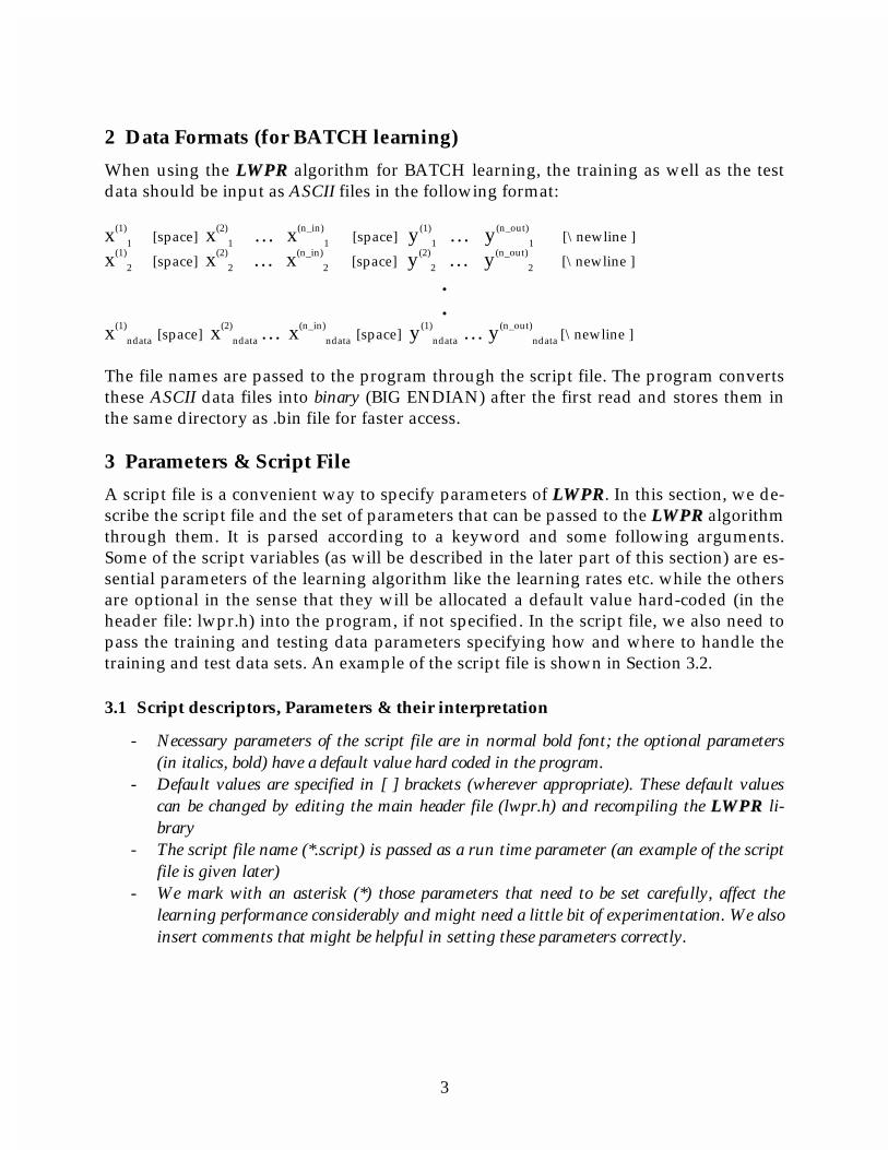
2 Data Formats (for BATCH learning)

When using the LLWWPPRR algorithm for BATCH learning, the training as well as the test data should be input as ASCII files in the following format: x(1)

1 [space] x(2)

1 … x(n_in)

1 [space] y(1)

1 … y(n_out)1 [\newline ]

x(1)2 [space] x

(2)2 … x

(n_in)2 [space] y

(2)2 … y(n_out)

2 [\newline ]

.

. x(1)

ndata [space] x(2)

ndata … x(n_in)

ndata [space] y(1)

ndata … y(n_out)ndata [\newline ]

The file names are passed to the program through the script file. The program converts these ASCII data files into binary (BIG ENDIAN) after the first read and stores them in the same directory as .bin file for faster access.

3 Parameters & Script File

A script file is a convenient way to specify parameters of LLWWPPRR. In this section, we de-scribe the script file and the set of parameters that can be passed to the LLWWPPRR algorithm through them. It is parsed according to a keyword and some following arguments. Some of the script variables (as will be described in the later part of this section) are es-sential parameters of the learning algorithm like the learning rates etc. while the others are optional in the sense that they will be allocated a default value hard-coded (in the header file: lwpr.h) into the program, if not specified. In the script file, we also need to pass the training and testing data parameters specifying how and where to handle the training and test data sets. An example of the script file is shown in Section 3.2.

3.1 Script descriptors, Parameters & their interpretation

- Necessary parameters of the script file are in normal bold font; the optional parameters (in italics, bold) have a default value hard coded in the program.

- Default values are specified in [ ] brackets (wherever appropriate). These default values can be changed by editing the main header file (lwpr.h) and recompiling the LLWWPPRR li-brary

- The script file name (*.script) is passed as a run time parameter (an example of the script file is given later)

- We mark with an asterisk (*) those parameters that need to be set carefully, affect the learning performance considerably and might need a little bit of experimentation. We also insert comments that might be helpful in setting these parameters correctly.

4

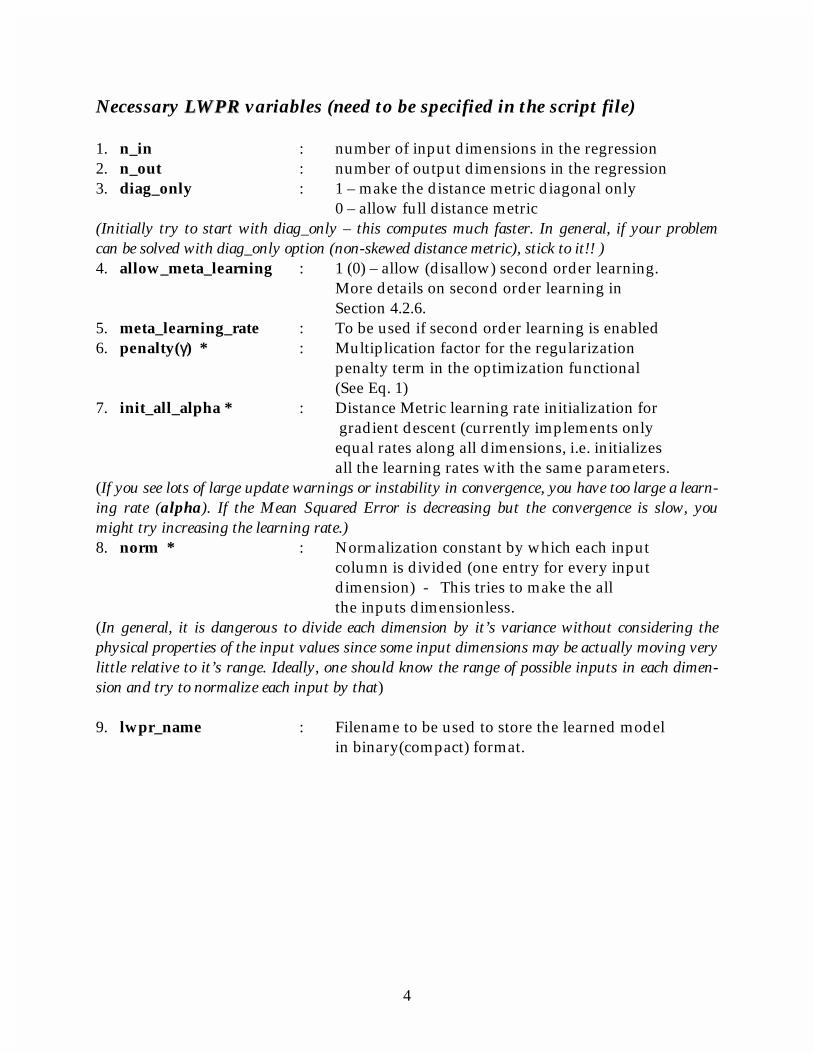
Necessary LLWWPPRR variables (need to be specified in the script file)

1. n_in : number of input dimensions in the regression 2. n_out : number of output dimensions in the regression 3. diag_only : 1 – make the distance metric diagonal only 0 – allow full distance metric (Initially try to start with diag_only – this computes much faster. In general, if your problem can be solved with diag_only option (non-skewed distance metric), stick to it!! ) 4. allow_meta_learning : 1 (0) – allow (disallow) second order learning. More details on second order learning in Section 4.2.6. 5. meta_learning_rate : To be used if second order learning is enabled 6. penalty(γ) * : Multiplication factor for the regularization penalty term in the optimization functional (See Eq. 1) 7. init_all_alpha * : Distance Metric learning rate initialization for gradient descent (currently implements only equal rates along all dimensions, i.e. initializes all the learning rates with the same parameters. (If you see lots of large update warnings or instability in convergence, you have too large a learn-ing rate (alpha). If the Mean Squared Error is decreasing but the convergence is slow, you might try increasing the learning rate.) 8. norm * : Normalization constant by which each input column is divided (one entry for every input dimension) - This tries to make the all the inputs dimensionless. (In general, it is dangerous to divide each dimension by it’s variance without considering the physical properties of the input values since some input dimensions may be actually moving very little relative to it’s range. Ideally, one should know the range of possible inputs in each dimen-sion and try to normalize each input by that) 9. lwpr_name : Filename to be used to store the learned model in binary(compact) format.

5

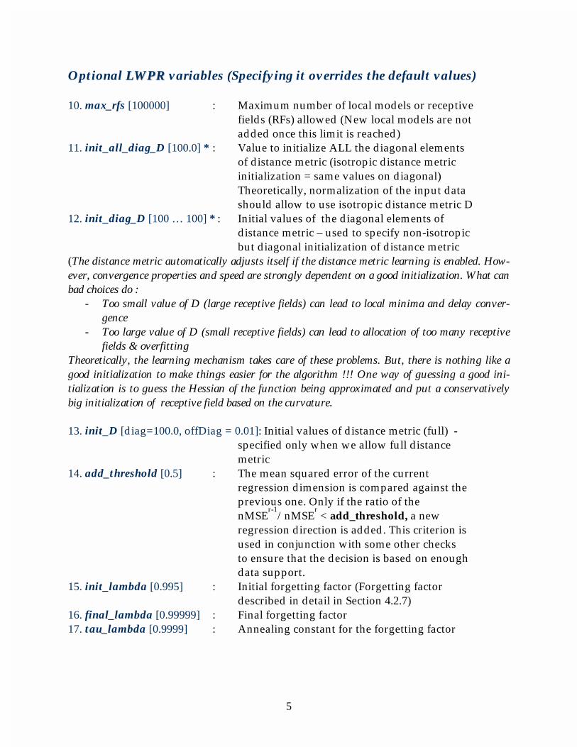
Optional LLWWPPRR variables (Specifying it overrides the default values) 10. max_rfs [100000] : Maximum number of local models or receptive fields (RFs) allowed (New local models are not added once this limit is reached) 11. init_all_diag_D [100.0] * : Value to initialize ALL the diagonal elements of distance metric (isotropic distance metric initialization = same values on diagonal) Theoretically, normalization of the input data should allow to use isotropic distance metric D 12. init_diag_D [100 … 100] * : Initial values of the diagonal elements of distance metric – used to specify non-isotropic but diagonal initialization of distance metric (The distance metric automatically adjusts itself if the distance metric learning is enabled. How-ever, convergence properties and speed are strongly dependent on a good initialization. What can bad choices do :

- Too small value of D (large receptive fields) can lead to local minima and delay conver-gence

- Too large value of D (small receptive fields) can lead to allocation of too many receptive fields & overfitting

Theoretically, the learning mechanism takes care of these problems. But, there is nothing like a good initialization to make things easier for the algorithm !!! One way of guessing a good ini-tialization is to guess the Hessian of the function being approximated and put a conservatively big initialization of receptive field based on the curvature. 13. init_D [diag=100.0, offDiag = 0.01]: Initial values of distance metric (full) - specified only when we allow full distance metric 14. add_threshold [0.5] : The mean squared error of the current regression dimension is compared against the previous one. Only if the ratio of the nMSE

r-1/nMSE

r < add_threshold, a new

regression direction is added. This criterion is used in conjunction with some other checks to ensure that the decision is based on enough data support. 15. init_lambda [0.995] : Initial forgetting factor (Forgetting factor described in detail in Section 4.2.7) 16. final_lambda [0.99999] : Final forgetting factor 17. tau_lambda [0.9999] : Annealing constant for the forgetting factor

6

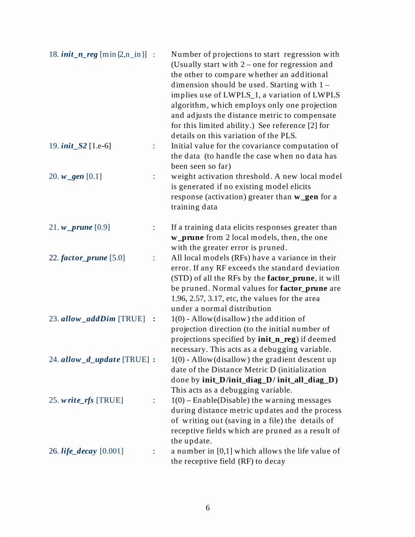
18. init_n_reg [min{2,n_in}] : Number of projections to start regression with (Usually start with 2 – one for regression and the other to compare whether an additional dimension should be used. Starting with 1 – implies use of LWPLS_1, a variation of LWPLS algorithm, which employs only one projection and adjusts the distance metric to compensate for this limited ability.) See reference [2] for details on this variation of the PLS. 19. init_S2 [1.e-6] : Initial value for the covariance computation of the data (to handle the case when no data has been seen so far) 20. w_gen [0.1] : weight activation threshold. A new local model is generated if no existing model elicits response (activation) greater than w_gen for a training data 21. w_prune [0.9] : If a training data elicits responses greater than w_prune from 2 local models, then, the one with the greater error is pruned. 22. factor_prune [5.0] : All local models (RFs) have a variance in their error. If any RF exceeds the standard deviation (STD) of all the RFs by the factor_prune, it will be pruned. Normal values for factor_prune are 1.96, 2.57, 3.17, etc, the values for the area under a normal distribution 23. allow_addDim [TRUE] : 1(0) - Allow(disallow) the addition of projection direction (to the initial number of projections specified by init_n_reg) if deemed necessary. This acts as a debugging variable. 24. allow_d_update [TRUE] : 1(0) - Allow(disallow) the gradient descent up date of the Distance Metric D (initialization done by init_D/init_diag_D/ init_all_diag_D) This acts as a debugging variable. 25. write_rfs [TRUE] : 1(0) – Enable(Disable) the warning messages during distance metric updates and the process of writing out (saving in a file) the details of receptive fields which are pruned as a result of the update. 26. life_decay [0.001] : a number in [0,1] which allows the life value of the receptive field (RF) to decay

7

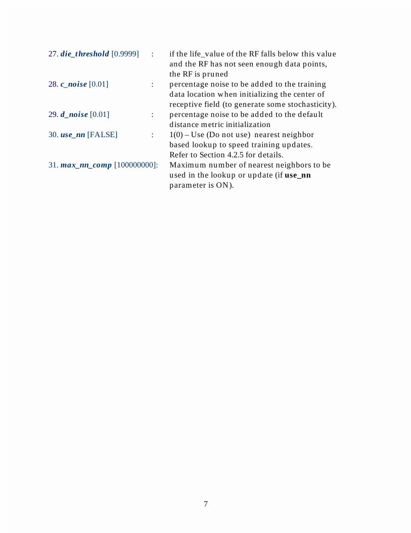
27. die_threshold [0.9999] : if the life_value of the RF falls below this value and the RF has not seen enough data points, the RF is pruned 28. c_noise [0.01] : percentage noise to be added to the training data location when initializing the center of receptive field (to generate some stochasticity). 29. d_noise [0.01] : percentage noise to be added to the default distance metric initialization 30. use_nn [FALSE] : 1(0) – Use (Do not use) nearest neighbor based lookup to speed training updates. Refer to Section 4.2.5 for details. 31. max_nn_comp [100000000]: Maximum number of nearest neighbors to be used in the lookup or update (if use_nn parameter is ON).

8

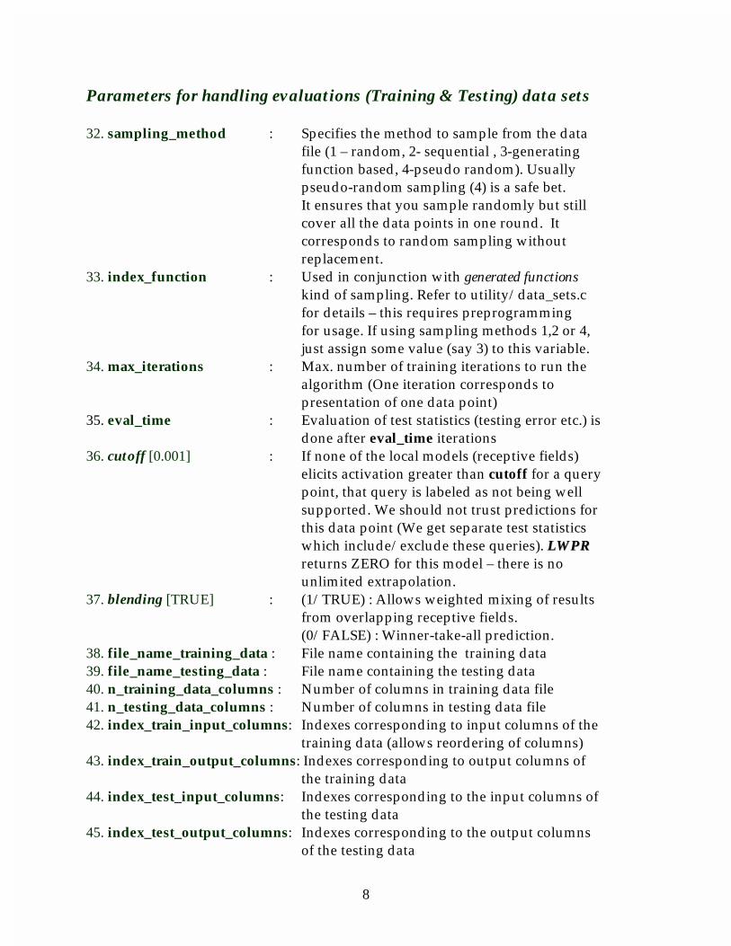
Parameters for handling evaluations (Training & Testing) data sets 32. sampling_method : Specifies the method to sample from the data file (1 – random, 2- sequential , 3-generating function based, 4-pseudo random). Usually pseudo-random sampling (4) is a safe bet. It ensures that you sample randomly but still cover all the data points in one round. It corresponds to random sampling without replacement. 33. index_function : Used in conjunction with generated functions kind of sampling. Refer to utility/data_sets.c for details – this requires preprogramming for usage. If using sampling methods 1,2 or 4, just assign some value (say 3) to this variable. 34. max_iterations : Max. number of training iterations to run the algorithm (One iteration corresponds to presentation of one data point) 35. eval_time : Evaluation of test statistics (testing error etc.) is done after eval_time iterations 36. cutoff [0.001] : If none of the local models (receptive fields) elicits activation greater than cutoff for a query point, that query is labeled as not being well supported. We should not trust predictions for this data point (We get separate test statistics which include/exclude these queries). LLWWPPRR returns ZERO for this model – there is no unlimited extrapolation. 37. blending [TRUE] : (1/TRUE) : Allows weighted mixing of results from overlapping receptive fields. (0/FALSE) : Winner-take-all prediction. 38. file_name_training_data : File name containing the training data 39. file_name_testing_data : File name containing the testing data 40. n_training_data_columns : Number of columns in training data file 41. n_testing_data_columns : Number of columns in testing data file 42. index_train_input_columns: Indexes corresponding to input columns of the training data (allows reordering of columns) 43. index_train_output_columns: Indexes corresponding to output columns of the training data 44. index_test_input_columns: Indexes corresponding to the input columns of the testing data 45. index_test_output_columns: Indexes corresponding to the output columns of the testing data

9

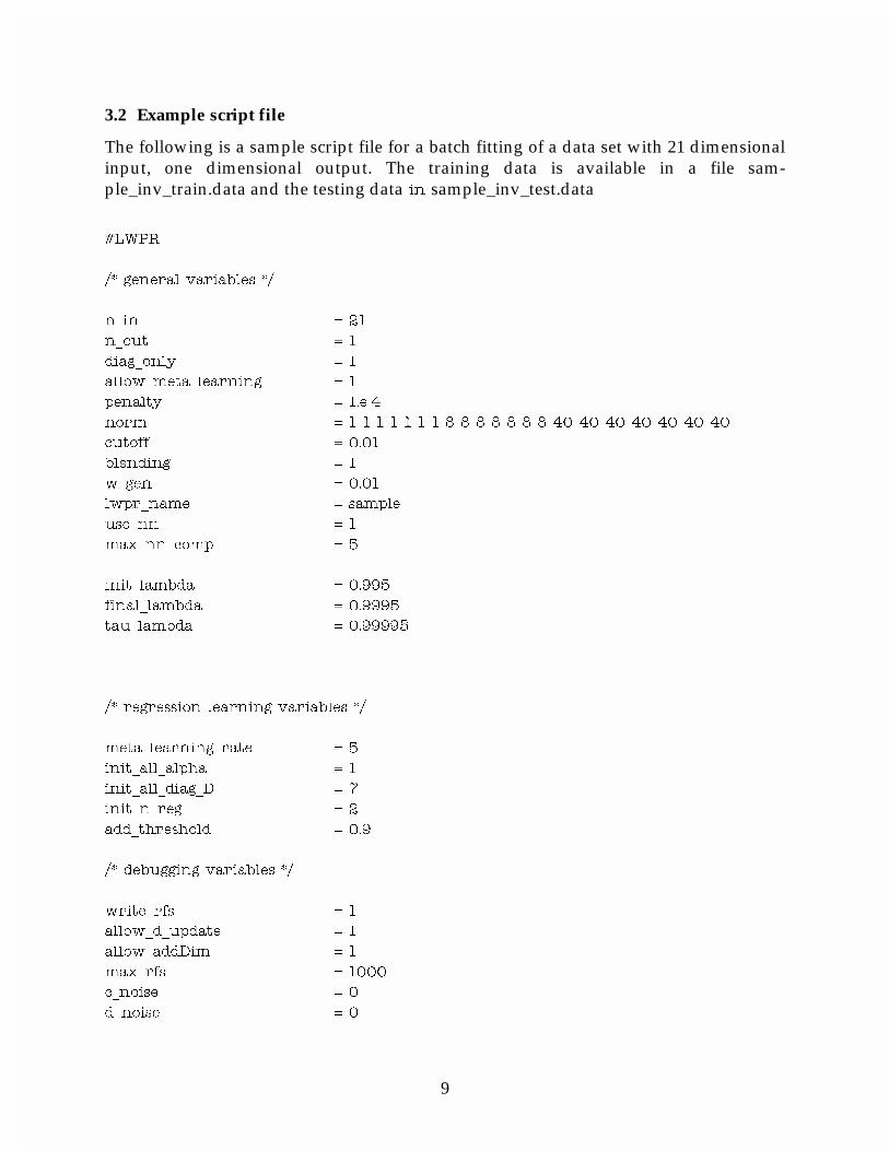
3.2 Example script file

The following is a sample script file for a batch fitting of a data set with 21 dimensional input, one dimensional output. The training data is available in a file sam-ple_inv_train.data and the testing data LQ sample_inv_test.data

�/:35

� JHQHUDO YDULDEOHV �

QBLQ ��

QBRXW �

GLDJBRQO\ �

DOORZBPHWDBOHDUQLQJ �

SHQDOW\ ��H��

QRUP � � � � � � � � � � � � � � �� �� �� �� �� �� ��

FXWRII ����

EOHQGLQJ �

ZBJHQ ����

OZSUBQDPH VDPSOH

XVHBQQ �

PD[BQQBFRPS �

LQLWBODPEGD �����

ILQDOBODPEGD ������

WDXBODPEGD �������

� UHJUHVVLRQ OHDUQLQJ YDULDEOHV �

PHWDBOHDUQLQJBUDWH �

LQLWBDOOBDOSKD �

LQLWBDOOBGLDJB' �

LQLWBQBUHJ �

DGGBWKUHVKROG ���

� GHEXJJLQJ YDULDEOHV �

ZULWHBUIV �

DOORZBGBXSGDWH �

DOORZBDGG'LP �

PD[BUIV ����

FBQRLVH �

GBQRLVH �

10

� GDWD VHW YDULDEOHV �

VDPSOLQJBPHWKRG �

LQGH[BIXQFWLRQ �

PD[BLWHUDWLRQV ������

HYDOBWLPH �����

ILOHBQDPHBWUDLQLQJBGDWD VDPSOHBLQYBWUDLQ�GDWD

ILOHBQDPHBWHVWLQJBGDWD VDPSOHBLQYBWHVW�GDWD

QBWUDLQLQJBGDWDBFROXPQV ��

QBWHVWLQJBGDWDBFROXPQV ��

LQGH[BWUDLQBLQSXWBFROXPQV � � � � � � � � � �� �� �� �� �� �� �� �� �� �� �� ��

LQGH[BWUDLQBRXWSXWBFROXPQV ��

LQGH[BWHVWBLQSXWBFROXPQV � � � � � � � � � �� �� �� �� �� �� �� �� �� �� �� ��

LQGH[BWHVWBRXWSXWBFROXPQV ��

11

4 Basic elements of the program code

4.1 The event loop

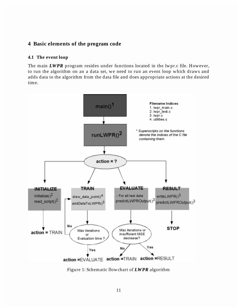
The main LLWWPPRR program resides under functions located in the lwpr.c file. However, to run the algorithm on an a data set, we need to run an event loop which draws and adds data to the algorithm from the data file and does appropriate actions at the desired time.

Figure 1: Schematic flowchart of LLWWPPRR algorithm

12

The structure of the event loop is shown in Fig.1. The algorithm is at one of the four action states at any given point of time. The INITIALIZE phase is used to initialize the LLWWPPRR and read in the script variables from the script file and fill in default values for those variables not specified in the script file.

The TRAIN phase of the algorithm draws data from the training data set file and trains the local model on it. The details of learning with addition of data (which consti-tute the major part of the program code) are described in detail in the next section.

After every eval_time iterations, the program goes into the EVALUATE phase where the learned model is tested against the novel (test) data set. Run time learning traces – which are described in detail in the section on tracing, evaluation & debugging – are generated to help track the progress of the algorithm.

When the number of iterations has exceeded the max_iterations count or the change of normalized mean squared error (nMSE) between the last EVALUATE phase and the current is below a THRESHOLD (specified in lwpr_test.c), the program goes into the RESULT phase. In the RESULT phase, it dumps (saves) the learned LLWWPPRR, saves the re-sult of evaluation on the test set in a *.res file and PAUSES (stops).

13

4.2 Details of the Main C-Routine

The main routine in the C-code is the one that incorporates the new data into the cur-rent learnt model (addDataToLWPR()). Fig.2 describes the schematic of this routine. Most of the details are self-explanatory and the code itself has extensive comments which show what is being handled at which stage. During training, the main tasks to be carried out includes updating all the trace variables (running mean, variance etc.), up-dating the projection direction and the regressions along these directions and updating the distance metric according to the cost function gradient. In addition, one also needs to check whether a new projection direction needs to be added, whether a new RF (local model) needs to be added or whether one needs to be pruned. We will briefly describe each of these subroutines in the next subsections.

Figure 2: Main addData routine of the LLWWPPRR code

14

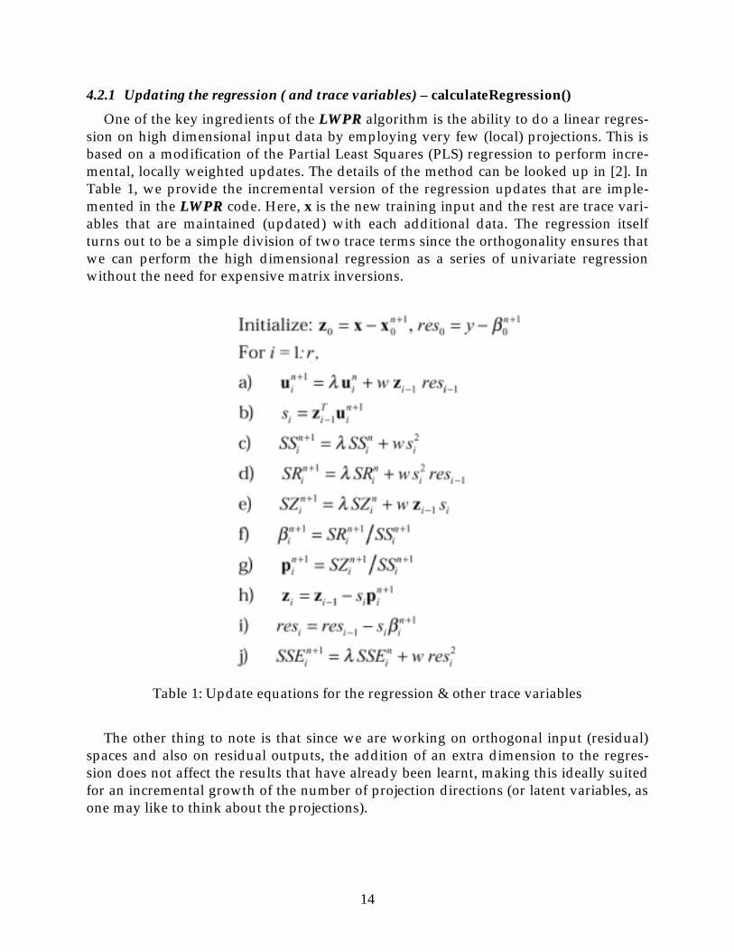
4.2.1 Updating the regression ( and trace variables) – calculateRegression()

One of the key ingredients of the LLWWPPRR algorithm is the ability to do a linear regres-sion on high dimensional input data by employing very few (local) projections. This is based on a modification of the Partial Least Squares (PLS) regression to perform incre-mental, locally weighted updates. The details of the method can be looked up in [2]. In Table 1, we provide the incremental version of the regression updates that are imple-mented in the LLWWPPRR code. Here, x is the new training input and the rest are trace vari-ables that are maintained (updated) with each additional data. The regression itself turns out to be a simple division of two trace terms since the orthogonality ensures that we can perform the high dimensional regression as a series of univariate regression without the need for expensive matrix inversions.

Table 1: Update equations for the regression & other trace variables

The other thing to note is that since we are working on orthogonal input (residual) spaces and also on residual outputs, the addition of an extra dimension to the regres-sion does not affect the results that have already been learnt, making this ideally suited for an incremental growth of the number of projection directions (or latent variables, as one may like to think about the projections).

∑∑ ∑== =

+

+

+−

=

−=

N

jiij

M

i

r

k

kTk

iki

ikit

tnn

D

Wss

sw

yw

WJwhere

�

��

1,

2

1 1 22

,

2,1,

cos

cos1

)1(

1

,

γ

α

res

DDD

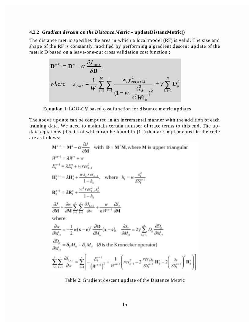
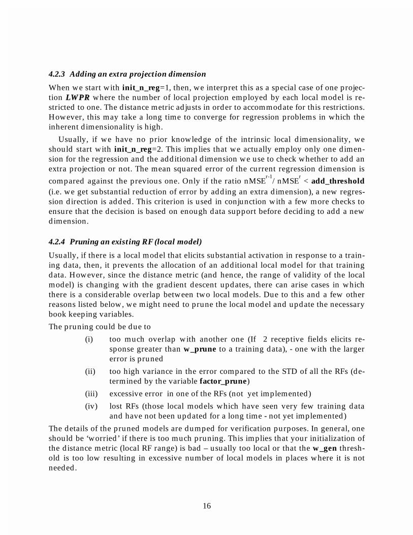
4.2.2 Gradient descent on the Distance Metric – updateDistancMetric()

The distance metric specifies the area in which a local model (RF) is valid. The size and shape of the RF is constantly modified by performing a gradient descent update of the metric D based on a leave-one-out cross validation cost function :

The atrainidate are as

s

Equation 1: LOO-CV based cost function for distance metric update

15

bove update can be computed in an incremental manner with the addition of each ng data. We need to maintain certain number of trace terms to this end. The up-equations (details of which can be found in [1] ) that are implemented in the code follows:

Table 2: Gradient descent update of the Distance Metric

16

4.2.3 Adding an extra projection dimension

When we start with init_n_reg=1, then, we interpret this as a special case of one projec-tion LLWWPPRR where the number of local projection employed by each local model is re-stricted to one. The distance metric adjusts in order to accommodate for this restrictions. However, this may take a long time to converge for regression problems in which the inherent dimensionality is high.

Usually, if we have no prior knowledge of the intrinsic local dimensionality, we should start with init_n_reg=2. This implies that we actually employ only one dimen-sion for the regression and the additional dimension we use to check whether to add an extra projection or not. The mean squared error of the current regression dimension is compared against the previous one. Only if the ratio nMSE

r-1/nMSE

r < add_threshold

(i.e. we get substantial reduction of error by adding an extra dimension), a new regres-sion direction is added. This criterion is used in conjunction with a few more checks to ensure that the decision is based on enough data support before deciding to add a new dimension.

4.2.4 Pruning an existing RF (local model)

Usually, if there is a local model that elicits substantial activation in response to a train-ing data, then, it prevents the allocation of an additional local model for that training data. However, since the distance metric (and hence, the range of validity of the local model) is changing with the gradient descent updates, there can arise cases in which there is a considerable overlap between two local models. Due to this and a few other reasons listed below, we might need to prune the local model and update the necessary book keeping variables.

The pruning could be due to

(i) too much overlap with another one (If 2 receptive fields elicits re-sponse greater than w_prune to a training data), - one with the larger error is pruned

(ii) too high variance in the error compared to the STD of all the RFs (de-termined by the variable factor_prune)

(iii) excessive error in one of the RFs (not yet implemented)

(iv) lost RFs (those local models which have seen very few training data and have not been updated for a long time - not yet implemented)

The details of the pruned models are dumped for verification purposes. In general, one should be ‘worried’ if there is too much pruning. This implies that your initialization of the distance metric (local RF range) is bad – usually too local or that the w_gen thresh-old is too low resulting in excessive number of local models in places where it is not needed.

17

4.2.5 Maintaining the local nearest neighbor (nn) list

When using the regression analysis in applications where the input values changes smoothly (i.e., do not jump around) – typically in movement systems like robots – it is useful to keep a neighborhood list and perform training by looking at only the neighboring local models which are close to each other or have a substantial overlap in their activation profiles. This saves a lot of computing resources as opposed to going through all the local models and finding out those that have enough activation to be updated.

Hence, it suffices to look at the neighborhood list to check for activations that are above the threshold and need to be updated.

4.2.6 Second order updates

The gradient descent updates of the distance metric is speeded up – faster convergence - and is more efficient if we use Newton’s second order gradient information (meta learn-ing) and incorporate this into the learning updates.

If the allow_meta_learning variable is TRUE, then the second order learning is switched on.

4.2.7 Forgetting factor

The forgetting factor is a variable that is used to discount the effects of the statistics computed at an earlier stage (when we had seen very few data points) and give more weight to the recent statistics - which are a result of having experienced more data points. It can be thought of as a sliding window over which the stochastic sufficient sta-tistics are accumulated.

The forgetting factor (lambda) takes a value [0,1] where 0 corresponds to using only the current point and 1 corresponding to not `forgetting ‘ anything. Here, we use an an-nealed forgetting rate which forgets more at the start (to account for unsettled learning dynamics) – specified by init_lambda and anneals towards a value closer to one (fi-nal_lambda) - not forgetting anything based on annealing factor tau_lambda.

18

5 Unpacking, Compiling and Creating Executables

Unpack the LLWWPPRR distribution (lwpr.tar.gz) using the gzip –d option and then, tar –xvf option under your home directory or wherever you want to install it (here, called /MYHOME for explanation purposes). This procedure will create a directory /MYHOME/lwpr and unpack all the files under this.

The /MYHOME/lwpr/src directory contains all the source files of the algorithm (like lwpr.c, lwpr.h etc.). There are machine specific subdirectories (like /lwpr/sparc, /lwpr/mac etc.) for putting the appropriate object files and executables for execution on different platforms. This installation of the executable to the appropriate machine specific directory is handled by the Makefile. Then, there is an /lwpr/Imakefile which is used for generating the Makefile for compiling the code. It is much easier and intui-tive to make changes in the Imakefile and automatically generate the Makefile from it as compared to directly trying to modify the Makefile.

19

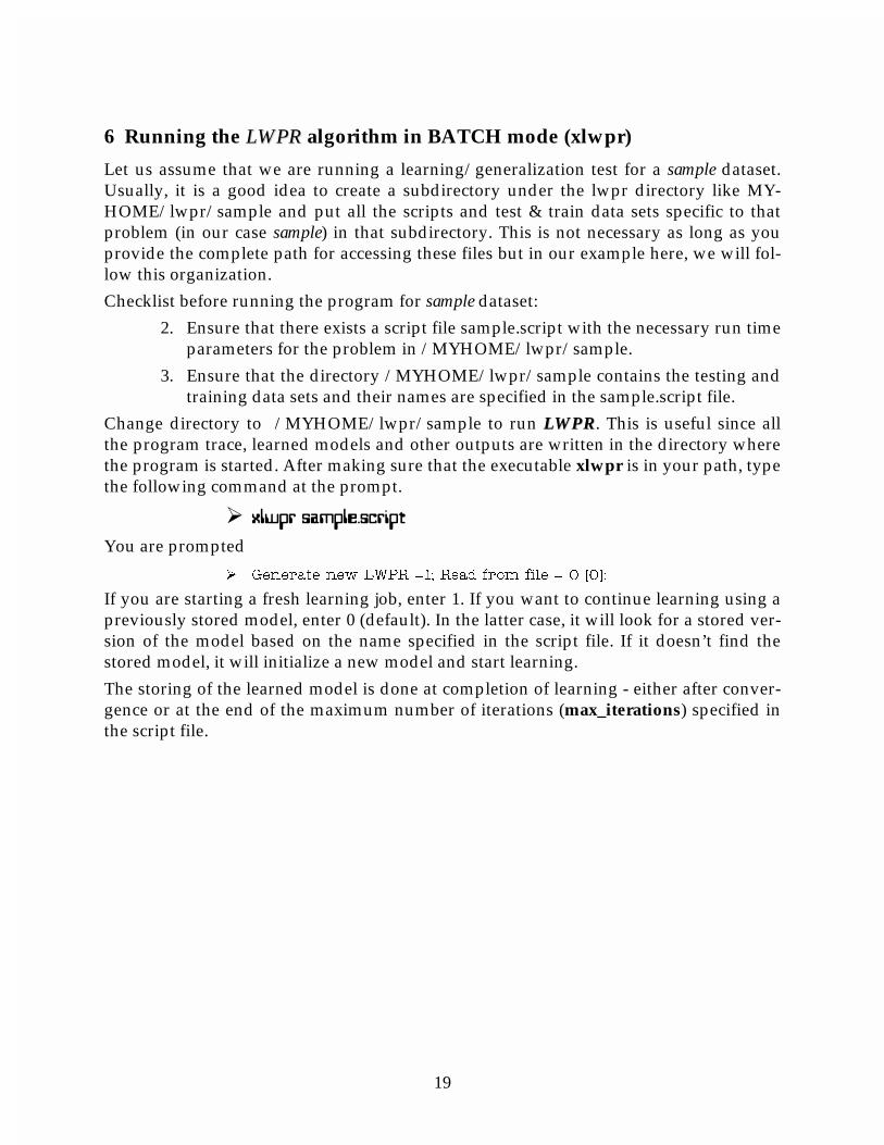
6 Running the LLWWPPRR algorithm in BATCH mode (xlwpr)

Let us assume that we are running a learning/generalization test for a sample dataset. Usually, it is a good idea to create a subdirectory under the lwpr directory like MY-HOME/lwpr/sample and put all the scripts and test & train data sets specific to that problem (in our case sample) in that subdirectory. This is not necessary as long as you provide the complete path for accessing these files but in our example here, we will fol-low this organization.

Checklist before running the program for sample dataset:

2. Ensure that there exists a script file sample.script with the necessary run time parameters for the problem in /MYHOME/lwpr/sample.

3. Ensure that the directory /MYHOME/lwpr/sample contains the testing and training data sets and their names are specified in the sample.script file.

Change directory to /MYHOME/lwpr/sample to run LLWWPPRR. This is useful since all the program trace, learned models and other outputs are written in the directory where the program is started. After making sure that the executable xlwpr is in your path, type the following command at the prompt.

���������������� ���

You are prompted

¾ *HQHUDWH QHZ /:35 �� 5HDG IURP ILOH � >�@�

If you are starting a fresh learning job, enter 1. If you want to continue learning using a previously stored model, enter 0 (default). In the latter case, it will look for a stored ver-sion of the model based on the name specified in the script file. If it doesn’t find the stored model, it will initialize a new model and start learning.

The storing of the learned model is done at completion of learning - either after conver-gence or at the end of the maximum number of iterations (max_iterations) specified in the script file.

20

7 Tracing and Evaluation in batch mode

In this section, we will concentrate on the features offered by LLWWPPRR for tracing the pro-gress of learning and evaluation mechanisms. We will systematically look at the out-puts produced by the algorithm and lay out methods of interpreting the results.

7.1 Runtime trace outputs

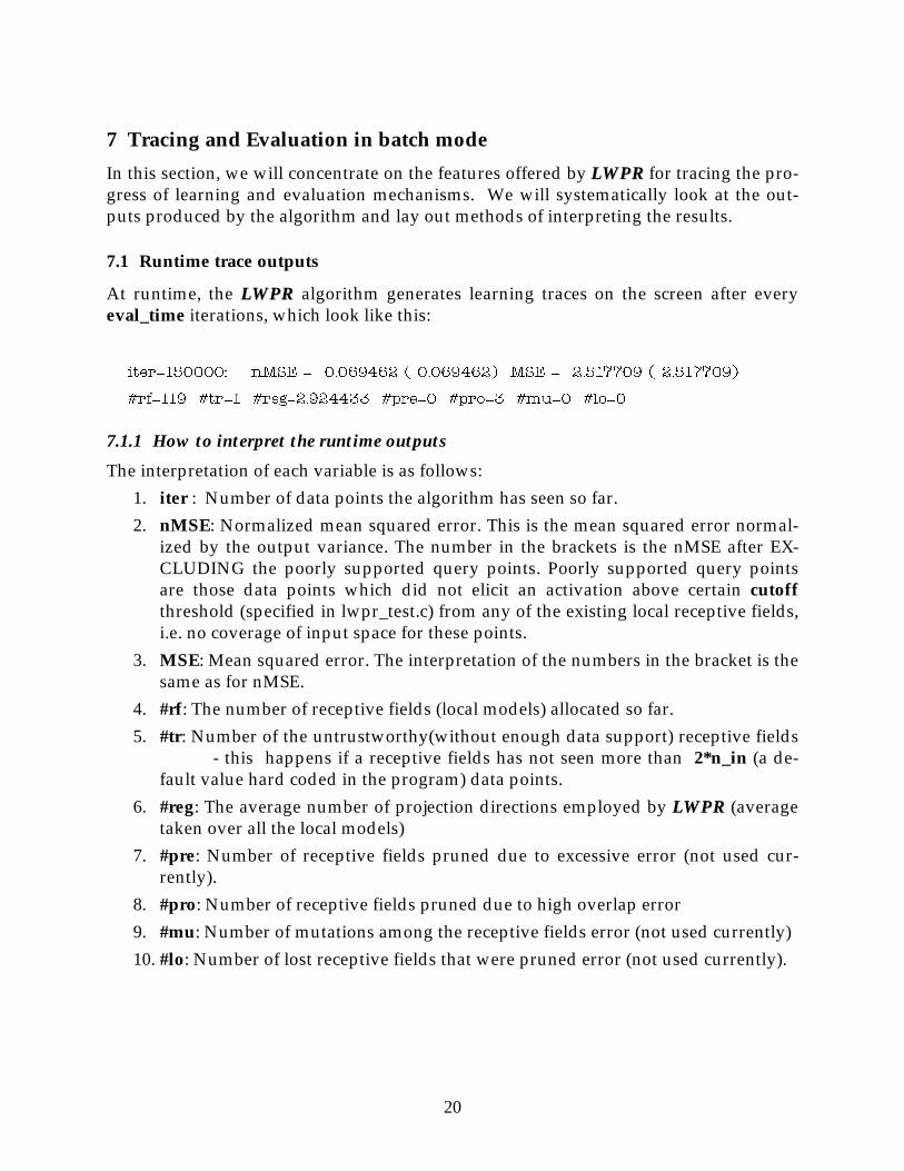
At runtime, the LLWWPPRR algorithm generates learning traces on the screen after every eval_time iterations, which look like this:

LWHU ������� Q06( �������� � ��������� 06( �������� � ���������

�UI ��� �WU � �UHJ �������� �SUH � �SUR � �PX � �OR �

7.1.1 How to interpret the runtime outputs

The interpretation of each variable is as follows:

1. iter : Number of data points the algorithm has seen so far.

2. nMSE: Normalized mean squared error. This is the mean squared error normal-ized by the output variance. The number in the brackets is the nMSE after EX-CLUDING the poorly supported query points. Poorly supported query points are those data points which did not elicit an activation above certain cutoff threshold (specified in lwpr_test.c) from any of the existing local receptive fields, i.e. no coverage of input space for these points.

3. MSE: Mean squared error. The interpretation of the numbers in the bracket is the same as for nMSE.

4. #rf: The number of receptive fields (local models) allocated so far.

5. #tr: Number of the untrustworthy(without enough data support) receptive fields - this happens if a receptive fields has not seen more than 2*n_in (a de-fault value hard coded in the program) data points.

6. #reg: The average number of projection directions employed by LLWWPPRR (average taken over all the local models)

7. #pre: Number of receptive fields pruned due to excessive error (not used cur-rently).

8. #pro: Number of receptive fields pruned due to high overlap error

9. #mu: Number of mutations among the receptive fields error (not used currently)

10. #lo: Number of lost receptive fields that were pruned error (not used currently).

21

7.1.2 Runtime warnings and error messages

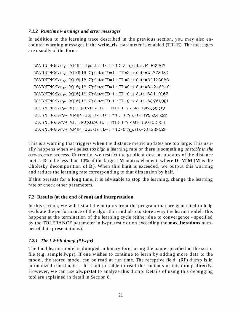
In addition to the learning trace described in the previous section, you may also en-counter warning messages if the write_rfs parameter is enabled (TRUE). The messages are usually of the form:

:$51,1*�/DUJH 0>�@>�@�8SGDWH� ,' � UI,' � QBGDWD ���������

:$51,1*�/DUJH 0>��@>��@�8SGDWH� ,' � UI,' � QBGDWD ���������

:$51,1*�/DUJH 0>��@>��@�8SGDWH� ,' � UI,' � QBGDWD ���������

:$51,1*�/DUJH 0>��@>��@�8SGDWH� ,' � UI,' � QBGDWD ���������

:$51,1*�/DUJH 0>��@>��@�8SGDWH� ,' � UI,' � QBGDWD ���������

:$51,1*�/DUJH 0>��@>��@�8SGDWH� ,' � UI,' � QBGDWD ���������

:$51,1*�/DUJH 0>�@>�@�8SGDWH� ,' � UI,' � QBGDWD ����������

:$51,1*�/DUJH 0>�@>�@�8SGDWH� ,' � UI,' � QBGDWD ����������

:$51,1*�/DUJH 0>�@>�@�8SGDWH� ,' � UI,' � QBGDWD ����������

:$51,1*�/DUJH 0>�@>�@�8SGDWH� ,' � UI,' � QBGDWD ����������

This is a warning that triggers when the distance metric updates are too large. This usu-ally happens when we select too high a learning rate or there is something unstable in the convergence process. Currently, we restrict the gradient descent updates of the distance metric D to be less than 10% of the largest M matrix element, where D=MTM (M is the Cholesky decomposition of D). When this limit is exceeded, we output this warning and reduce the learning rate corresponding to that dimension by half.

If this persists for a long time, it is advisable to stop the learning, change the learning rate or check other parameters.

7.2 Results (at the end of run) and interpretation

In this section, we will list all the outputs from the program that are generated to help evaluate the performance of the algorithm and also to store away the learnt model. This happens at the termination of the learning cycle (either due to convergence - specified by the TOLERANCE parameter in lwpr_test.c or on exceeding the max_iterations num-ber of data presentations).

7.2.1 The LLWWPPRR dump (*.lwpr)

The final learnt model is dumped in binary form using the name specified in the script file (e.g. sample.lwpr). If one wishes to continue to learn by adding more data to the model, the stored model can be read at run time. The receptive field (RF) dump is in normalized coordinates. It is not possible to read the contents of this dump directly. However, we can use xlwprstat to analyze this dump. Details of using this debugging tool are explained in detail in Section 8.

22

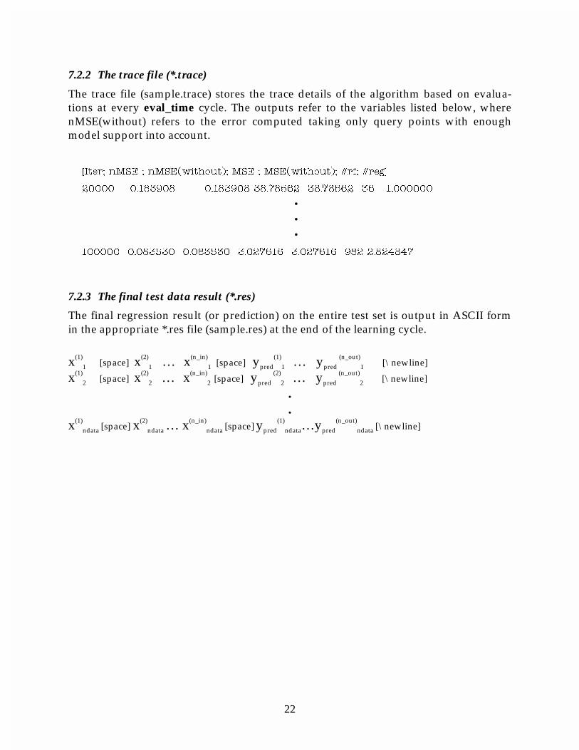
7.2.2 The trace file (*.trace)

The trace file (sample.trace) stores the trace details of the algorithm based on evalua-tions at every eval_time cycle. The outputs refer to the variables listed below, where nMSE(without) refers to the error computed taking only query points with enough model support into account.

>,WHU� Q06( � Q06(�ZLWKRXW�� 06( � 06(�ZLWKRXW�� �UI� �UHJ@

����� �������� �������� �������� �������� �� ��������

•

••

������ �������� �������� �������� �������� ��� ��������

7.2.3 The final test data result (*.res)

The final regression result (or prediction) on the entire test set is output in ASCII form in the appropriate *.res file (sample.res) at the end of the learning cycle.

x(1)

1 [space] x(2)

1 … x(n_in)

1 [space] ypred(1)

1 … ypred (n_out)

1 [\newline]

x(1)2 [space] x

(2)2 … x

(n_in)2 [space] ypred

(2)2 … ypred

(n_out)2 [\newline]

.

. x(1)

ndata [space] x(2)

ndata … x(n_in)ndata [space] ypred

(1)ndata…ypred

(n_out)ndata [\newline]

23

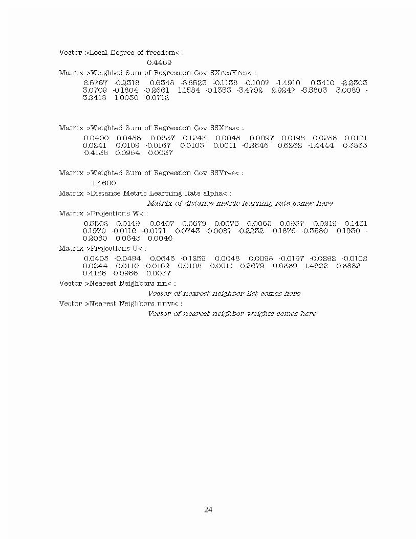
7.2.4 Pruned receptive filed dumps

If the write_rfs parameter is TRUE (default), then, whenever a receptive field is pruned, the details of the pruned local model are dumped into a file whose name is derived from the LLWWPPRR and the ID number of pruned receptive field. In addition to this, the de-tails of the receptive field that caused the pruning are also dumped. The pruning could be due to various factors that are described in detail in Section 4.2.4.

In the case when RF number 99 of the `sample’ LLWWPPRR is pruned due to excessive over-lap, an ASCII (readable) dump by the name sample.99.rf is generated which has the fol-lowing details:

�

'DWD RI 5) ��� RI /:35 !VDPSOH��

PHVVDJH RYHUODS SUXQH GXH WR ��

QBUHJ �

FRVW �����������

WUXVWZRUWK\ �

��VXPBZHLJKWV ���������

��VXPBHUURU ���������

��QBGDWD ����������

��ODPEGD ��������

VXPB'� ��������

QBXSGDWHV ����

OLIHBYDOXH ��������

9HFWRU !5)�FHQWHU F� �

YHFWRU FRPHV KHUH

0DWUL[ !5HJUHVVLRQ &RHIILFLHQWV %� �

������

0DWUL[ !0HPRU\ WUDFH +� �

�������

9HFWRU !0HPRU\ WUDFH U� �

������

0DWUL[ !'LVWDQFH 0HWULF '� �

'LVWDQFH PHWULF PDWUL[ FRPHV KHUH

9HFWRU !0HDQ LQ ,QSXW 6SDFH PHDQB[� �

:HLJKWHG PHDQ FRPHV KHUH

9HFWRU !9DU LQ ,QSXW 6SDFH PHDQB[� �

9DULDQFH RI GDWD VHHQ VR IDU FRPHV KHUH

9HFWRU !0HDQ LQ 2XWSXW 6SDFH PHDQB\� �

������

9HFWRU !9DU LQ 2XWSXW 6SDFH YDUB\� �

������

9HFWRU !:HLJKWHG 6XP RI 5HJUHVVLRQ 9DU VV�� �

������

24

9HFWRU !/RFDO 'HJUHH RI IUHHGRP� �

������

0DWUL[ !:HLJKWHG 6XP RI 5HJUHVVLRQ &RY 6;UHV<UHV� �

������ ������� ������ ������� ������� ������� ������� ������ ������������� ������� ������� ������ ������� ������� ������ ������� ������ ������� ������ �������

0DWUL[ !:HLJKWHG 6XP RI 5HJUHVVLRQ &RY 66;UHV� �

������ ������� ������ ������� ������ ������ ������� ������� ������������� ������ ������� ������ ������ ������� ������ ������� ������������� ������� ������

0DWUL[ !:HLJKWHG 6XP RI 5HJUHVVLRQ &RY 66<UHV� �

������

0DWUL[ !'LVWDQFH 0HWULF /HDUQLQJ 5DWH DOSKD� �

0DWUL[ RI GLVWDQFH PHWULF OHDUQLQJ UDWH FRPHV KHUH

0DWUL[ !3URMHFWLRQV :� �

������ ������� ������ ������� ������� ������� ������� ������ ������������� ������� ������� ������ ������� ������� ������ ������� ������ ������� ������ �������

0DWUL[ !3URMHFWLRQV 8� �

������ ������� ������ ������� ������ ������ ������� ������� ������������� ������ ������� ������ ������ ������� ������ ������� ������ ������� ������� ������

9HFWRU !1HDUHVW 1HLJKERUV QQ� �

9HFWRU RI QHDUHVW QHLJKERU OLVW FRPHV KHUH

9HFWRU !1HDUHVW 1HLJKERUV QQZ� �

9HFWRU RI QHDUHVW QHLJKERU ZHLJKWV FRPHV KHUH

25

8 DEBUG-ing the learnt LLWWPPRR model (xlwprstat)

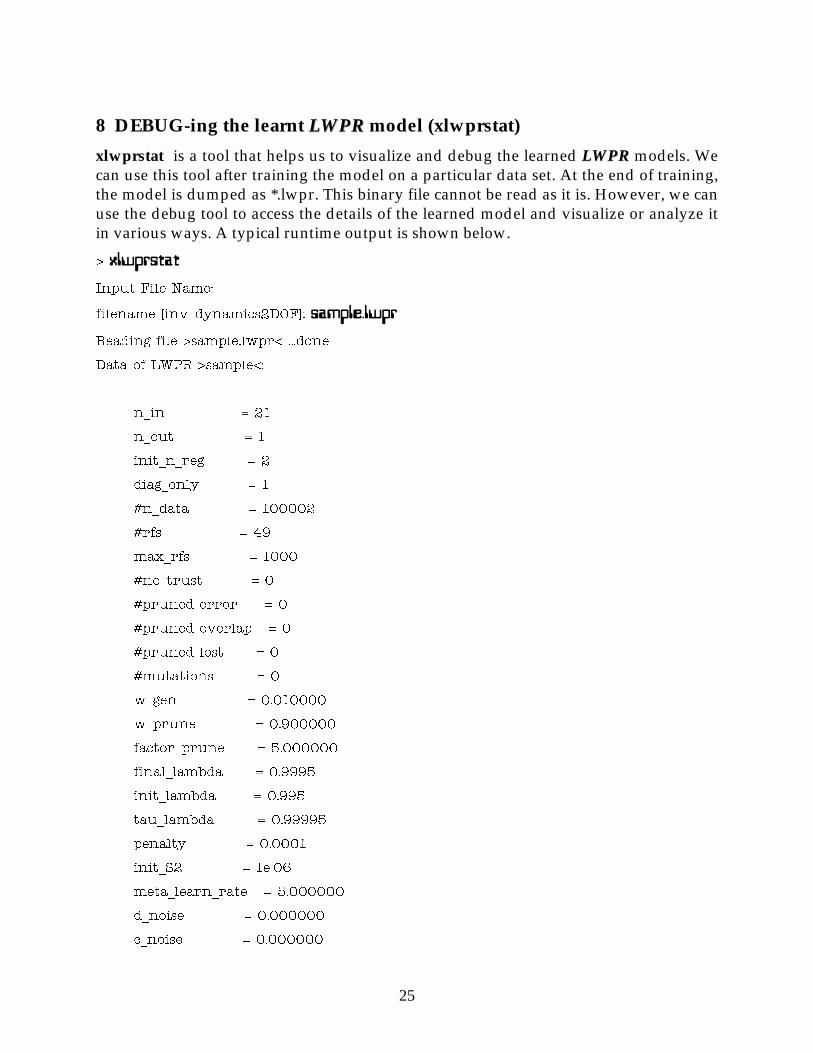
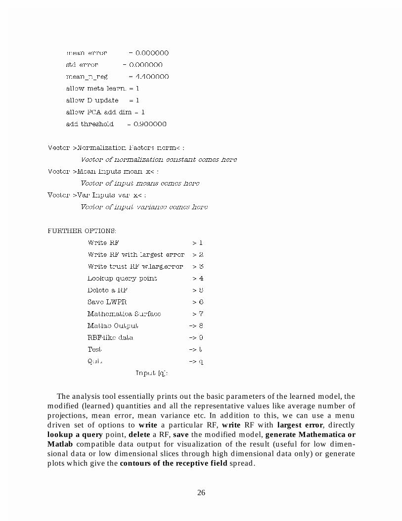
xlwprstat is a tool that helps us to visualize and debug the learned LLWWPPRR models. We can use this tool after training the model on a particular data set. At the end of training, the model is dumped as *.lwpr. This binary file cannot be read as it is. However, we can use the debug tool to access the details of the learned model and visualize or analyze it in various ways. A typical runtime output is shown below.

! ����������

,QSXW )LOH 1DPH�

ILOHQDPH >LQYBG\QDPLFV�'2)@� ���������

5HDGLQJ ILOH !VDPSOH�OZSU� ���GRQH

'DWD RI /:35 !VDPSOH��

QBLQ ��

QBRXW �

LQLWBQBUHJ �

GLDJBRQO\ �

�QBGDWD ������

�UIV ��

PD[BUIV ����

�QRBWUXVW �

�SUXQHG HUURU �

�SUXQHG RYHUODS �

�SUXQHG ORVW �

�PXWDWLRQV �

ZBJHQ ��������

ZBSUXQH ��������

IDFWRUBSUXQH ��������

ILQDOBODPEGD ������

LQLWBODPEGD �����

WDXBODPEGD �������

SHQDOW\ ������

LQLWB6� �H���

PHWDBOHDUQBUDWH ��������

GBQRLVH ��������

FBQRLVH ��������

26

PHDQBHUURU ��������

VWGBHUURU ��������

PHDQBQBUHJ ��������

DOORZ PHWD OHDUQ� �

DOORZ ' XSGDWH �

DOORZ 3&$ DGG GLP �

DGG WKUHVKROG ��������

9HFWRU !1RUPDOL]DWLRQ )DFWRUV QRUP� �

9HFWRU RI QRUPDOL]DWLRQ FRQVWDQW FRPHV KHUH

9HFWRU !0HDQ ,QSXWV PHDQB[� �

9HFWRU RI LQSXW PHDQV FRPHV KHUH

9HFWRU !9DU ,QSXWV YDUB[� �

9HFWRU RI LQSXW YDULDQFH FRPHV KHUH

)857+(5 237,216�

:ULWH 5) ��! �

:ULWH 5) ZLWK ODUJHVW HUURU ��! �

:ULWH WUXVW 5) Z�ODUJ�HUURU ��! �

/RRNXS TXHU\ SRLQW ��! �

'HOHWH D 5) ��! �

6DYH /:35 ��! �

0DWKHPDWLFD 6XUIDFH ��! �

0DWODE 2XWSXW ��! �

5%)�OLNH GDWD ��! �

7HVW ��! W

4XLW ��! T

,QSXW >T@�

The analysis tool essentially prints out the basic parameters of the learned model, the modified (learned) quantities and all the representative values like average number of projections, mean error, mean variance etc. In addition to this, we can use a menu driven set of options to write a particular RF, write RF with largest error, directly lookup a query point, delete a RF, save the modified model, generate Mathematica or Matlab compatible data output for visualization of the result (useful for low dimen-sional data or low dimensional slices through high dimensional data only) or generate plots which give the contours of the receptive field spread.

27

9 Embedding LLWWPPRR in an ONLINE real time system

There are some key functions that one will need to embed in their real time learning system to utilize the algorithm as an online incremental learning scheme. We will briefly describe what each of these functions achieves.

1. addDataToLWPR() : This function is the main routine involved in the learning phase. As described in detail in Section 4.2, it is this function that incrementally incorporates the new training data into the model and updates the necessary learning parameters. In a real time system, one should send the training data (in-put–output pairs) to this module at a frequency that can be afforded by your real-time computational constraints.

2. predictLWPROutput() : This function generates a prediction (output) for a given input data using the current model. For some problems where you need to predict on the same data that you used for training, a more efficient way (than doing the training and prediction separately) is to use the addDataToLWPRPre-dict() function which combines the above two functions. Generally, in online time critical implementations, the lookup or prediction has to be done with a higher priority than adding data to the learning system.

In addition to these critical functions that needs to be run continuously for real time operations, there are additional initialization and bookkeeping operations that need to be done. Some essential functions that are run primarily either at the start or end of the learning/predictions are listed here:

3. readLWPRScript() : This function reads the script file and parses the inputs based on some keywords. It is through this file that we pass the learning parame-ters to the real time learning system. This script is read when a new LWPR model is initialized.

4. writeLWPR() : This function dumps the final learnt module in binary form for future use. Debugging on this can be done using the xlwprstat executable.

5. readLWPR() : Using this function, any previously generated model that has been saved can be loaded and used for further learning or just prediction.

By embedding these sets of functions in a real time system, one can achieve the nec-essary online learning performance within the limits of the computational capabilities of the system.

28

10 Bibliography

1. Stefan Schaal, Chris Atkeson & Sethu Vijayakumar, Scalable Locally Weighted Statistical Tech-niques for Real Time Robot Learning, Applied Intelligence: Special Issue on Scalable Robotic Ap-plications of Neural Elsevier Science (in press).

2. Sethu Vijayakumar & Stefan Schaal, LWPR: An O(n) Algorithm for Incremental Real Time Learn-ing in High Dimensional Space, Proc. International Conference on Machine Learning (ICML2000), Stanford, CA pp.1079-1086 (2000).

3. Sethu Vijayakumar & Stefan Schaal, Real Time Learning in Humanoids: A challenge for scalabil-ity of Online Algorithms, Humanoids2000, First IEEE-RAS Intl. Conf. on Humanoid Robots MIT, Cambridge, MA, USA (2000).

4. Schaal, S. & Atkeson, C. G. "Constructive incremental learning from only local information." Neu-ral Computation, 10, 8, pp.2047-2084 (1998).