LOCALISED GENERATIVE FLOWS - OpenReview

Under review as a conference paper at ICLR 2020

LOCALISED GENERATIVE FLOWS

Anonymous authorsPaper under double-blind review

ABSTRACT

We argue that flow-based density models based on continuous bijections are lim-ited in their ability to learn target distributions with complicated topologies, andpropose localised generative flows (LGFs) to address this problem. LGFs are com-posed of stacked continuous mixtures of bijections, which enables each bijectionto learn a local region of the target rather than its entirety. Our method is a gener-alisation of existing flow-based methods, which can be used without modificationas the basis for an LGF model. Unlike normalising flows, LGFs do not permitexact computation of log likelihoods, but we propose a simple variational schemethat performs well in practice. We show empirically that LGFs yield improvedperformance across a variety of density estimation tasks.

1 INTRODUCTION

Flow-based generative models, often referred to as normalising flows, have become popular methodsfor density estimation because of their flexibility, expressiveness, and tractable likelihoods. Giventhe problem of learning an unknown target density p?X on a data space X , normalising flows modelp?X as the marginal of X obtained by the generative process

Z ∼ pZ , X := g−1(Z), (1)where pZ is a prior density on a space Z , and g : X → Z is a bijection.1 Assuming sufficientregularity, it follows thatX has density pX(x) = pZ(g(x))|detDg(x)| (see e.g. Billingsley (2008)).The parameters of g can be learned via maximum likelihood given i.i.d. samples from p?X .

To be effective, a normalising flow model must specify an expressive family of bijections withtractable Jacobians. Affine coupling layers (Dinh et al., 2014; 2016), autoregressive transformations(Germain et al., 2015; Papamakarios et al., 2017), ODE-based transformations (Grathwohl et al.,2018), and invertible ResNet blocks (Behrmann et al., 2019) are all examples of such bijectionsthat can be composed to produce complicated flows. These models have demonstrated significantpromise in their ability to model complex datasets (Papamakarios et al., 2017) and to synthesisenovel data points (Kingma & Dhariwal, 2018).

However, in all these cases, g is continuous in x. We believe this is a significant limitation of thesemodels since it imposes a global constraint on g−1, which must learn to match the topology of Z ,which is usually quite simple, to the topology of X , which we expect to be very complicated. We ar-gue that this constraint makes maximum likelihood estimation extremely difficult in general, leadingto training instabilities and erroneous regions of high likelihood in the learned density landscape.

To address this problem we introduce localised generative flows (LGFs), which generalise equation 1by replacing the single bijection g with stacked continuous mixtures of bijections {G(·;u)}u∈U foran index set U . Intuitively, LGFs allow each G(·;u) to focus on modelling only a local componentof the target that may have a much simpler topology than the full density. LGFs do not stipulatethe form of G, and indeed any standard choice of g can be used as the basis of its definition. Wepay a price for these benefits in that we can no longer compute the likelihood of our model exactlyand must instead resort to a variational approximation, with our training objective replaced by theevidence lower bound (ELBO). However, in practice we find this is not a significant limitation, asthe bijective structure of LGFs permits learning a high-quality variational distribution suitable forlarge-scale training. We show empirically that LGFs outperform their counterpart normalising flowsacross a variety of density estimation tasks.

1We assume throughout that X ,Z ⊆ Rd, and that all densities are with respect to the Lebesgue measure.

1


2 1 0 1 2

1.0

0.5

0.0

0.5

1.0

0.000

0.045

0.090

0.135

0.180

0.225

0.270

0.315

0.360

0.405

2 1 0 1 2

1.0

0.5

0.0

0.5

1.0

0.000

0.045

0.090

0.135

0.180

0.225

0.270

0.315

0.360

0.405

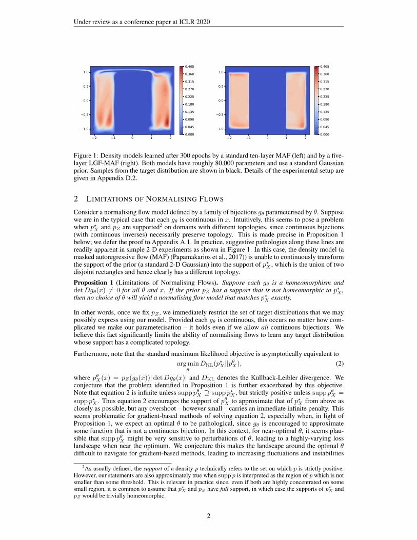
Figure 1: Density models learned after 300 epochs by a standard ten-layer MAF (left) and by a five-layer LGF-MAF (right). Both models have roughly 80,000 parameters and use a standard Gaussianprior. Samples from the target distribution are shown in black. Details of the experimental setup aregiven in Appendix D.2.

2 LIMITATIONS OF NORMALISING FLOWS

Consider a normalising flow model defined by a family of bijections gθ parameterised by θ. Supposewe are in the typical case that each gθ is continuous in x. Intuitively, this seems to pose a problemwhen p?X and pZ are supported2 on domains with different topologies, since continuous bijections(with continuous inverses) necessarily preserve topology. This is made precise in Proposition 1below; we defer the proof to Appendix A.1. In practice, suggestive pathologies along these lines arereadily apparent in simple 2-D experiments as shown in Figure 1. In this case, the density model (amasked autoregressive flow (MAF) (Papamakarios et al., 2017)) is unable to continuously transformthe support of the prior (a standard 2-D Gaussian) into the support of p?X , which is the union of twodisjoint rectangles and hence clearly has a different topology.

Proposition 1 (Limitations of Normalising Flows). Suppose each gθ is a homeomorphism anddetDgθ(x) 6= 0 for all θ and x. If the prior pZ has a support that is not homeomorphic to p∗X ,then no choice of θ will yield a normalising flow model that matches p∗X exactly.

In other words, once we fix pZ , we immediately restrict the set of target distributions that we maypossibly express using our model. Provided each gθ is continuous, this occurs no matter how com-plicated we make our parameterisation – it holds even if we allow all continuous bijections. Webelieve this fact significantly limits the ability of normalising flows to learn any target distributionwhose support has a complicated topology.

Furthermore, note that the standard maximum likelihood objective is asymptotically equivalent toarg min

θDKL(p?X ||pθX), (2)

where pθX(x) = pZ(gθ(x))|detDgθ(x)| and DKL denotes the Kullback-Leibler divergence. Weconjecture that the problem identified in Proposition 1 is further exacerbated by this objective.Note that equation 2 is infinite unless supp pθX ⊇ supp p?X , but strictly positive unless supp pθX =supp p?X . Thus equation 2 encourages the support of pθX to approximate that of p?X from above asclosely as possible, but any overshoot – however small – carries an immediate infinite penalty. Thisseems problematic for gradient-based methods of solving equation 2, especially when, in light ofProposition 1, we expect an optimal θ to be pathological, since gθ is encouraged to approximatesome function that is not a continuous bijection. In this context, for near-optimal θ, it seems plau-sible that supp pθX might be very sensitive to perturbations of θ, leading to a highly-varying losslandscape when near the optimum. We conjecture this makes the landscape around the optimal θdifficult to navigate for gradient-based methods, leading to increasing fluctuations and instabilities

2As usually defined, the support of a density p technically refers to the set on which p is strictly positive.However, our statements are also approximately true when supp p is interpreted as the region of p which is notsmaller than some threshold. This is relevant in practice since, even if both are highly concentrated on somesmall region, it is common to assume that p?X and pZ have full support, in which case the supports of p?X andpZ would be trivially homeomorphic.

2


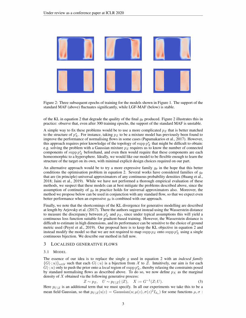
Figure 2: Three subsequent epochs of training for the models shown in Figure 1. The support of thestandard MAF (above) fluctuates significantly, while LGF-MAF (below) is stable.

of the KL in equation 2 that degrade the quality of the final gθ produced. Figure 2 illustrates this inpractice: observe that, even after 300 training epochs, the support of the standard MAF is unstable.

A simple way to fix these problems would be to use a more complicated pZ that is better matchedto the structure of p?X . For instance, taking pZ to be a mixture model has previously been found toimprove the performance of normalising flows in some cases (Papamakarios et al., 2017). However,this approach requires prior knowledge of the topology of supp p?X that might be difficult to obtain:e.g. solving the problem with a Gaussian mixture pZ requires us to know the number of connectedcomponents of supp p?X beforehand, and even then would require that these components are eachhomeomorphic to a hypersphere. Ideally, we would like our model to be flexible enough to learn thestructure of the target on its own, with minimal explicit design choices required on our part.

An alternative approach would be to try a more expressive family gθ in the hope that this betterconditions the optimisation problem in equation 2. Several works have considered families of gθthat are (in principle) universal approximators of any continuous probability densities (Huang et al.,2018; Jaini et al., 2019). While we have not performed a thorough empirical evaluation of thesemethods, we suspect that these models can at best mitigate the problems described above, since theassumption of continuity of gθ in practice holds for universal approximators also. Moreover, themethod we propose below can be used in conjunction with any standard flow, so that we expect evenbetter performance when an expressive gθ is combined with our approach.

Finally, we note that the shortcomings of the KL divergence for generative modelling are describedat length by Arjovsky et al. (2017). There the authors suggest instead using the Wasserstein distanceto measure the discrepancy between p?X and pZ , since under typical assumptions this will yield acontinuous loss function suitable for gradient-based training. However, the Wasserstein distance isdifficult to estimate in high dimensions, and its performance can be sensitive to the choice of groundmetric used (Peyre et al., 2019). Our proposal here is to keep the KL objective in equation 2 andinstead modify the model so that we are not required to map supp pZ onto supp p?X using a singlecontinuous bijection. We describe our method in full now.

3 LOCALISED GENERATIVE FLOWS

3.1 MODEL

The essence of our idea is to replace the single g used in equation 2 with an indexed family{G(·;u)}u∈U such that each G(·;u) is a bijection from X to Z . Intuitively, our aim is for eachG(·;u) only to push the prior onto a local region of supp p?X , thereby relaxing the constraints posedby standard normalising flows as described above. To do so, we now define pX as the marginaldensity of X obtained via the following generative process:

Z ∼ pZ , U ∼ pU |Z(·|Z), X := G−1(Z;U). (3)Here pU |Z is an additional term that we must specify. In all our experiments we take this to be amean field Gaussian, so that pU |Z(u|z) = Gaussian(u;µ(z), σ(z)2Idu) for some functions µ, σ :

3


��−1�1

�1 ��−1

...�0 �

(a) Generative Model

��−1�1

�1 ��−1 ��0

...

(b) Inference Model

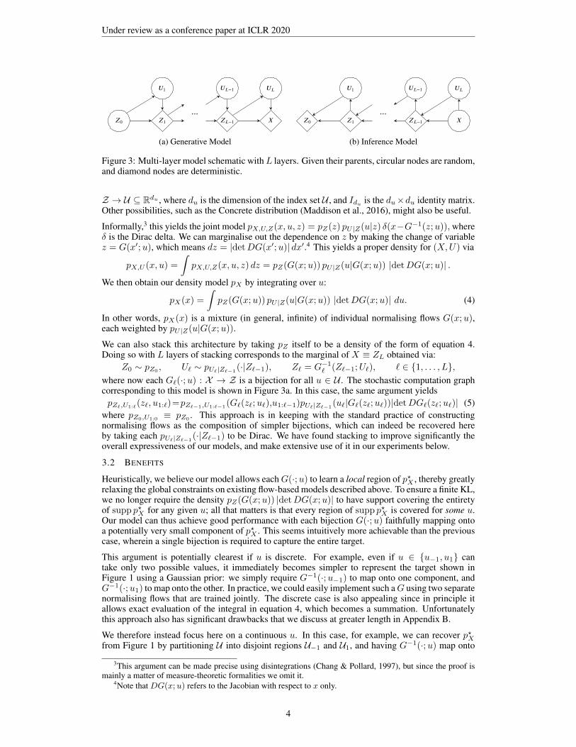
Figure 3: Multi-layer model schematic withL layers. Given their parents, circular nodes are random,and diamond nodes are deterministic.

Z → U ⊆ Rdu , where du is the dimension of the index set U , and Idu is the du×du identity matrix.Other possibilities, such as the Concrete distribution (Maddison et al., 2016), might also be useful.

Informally,3 this yields the joint model pX,U,Z(x, u, z) = pZ(z) pU |Z(u|z) δ(x−G−1(z;u)),whereδ is the Dirac delta. We can marginalise out the dependence on z by making the change of variablez = G(x′;u), which means dz = |detDG(x′;u)| dx′.4 This yields a proper density for (X,U) via

pX,U (x, u) =

∫pX,U,Z(x, u, z) dz = pZ(G(x;u)) pU |Z(u|G(x;u)) |detDG(x;u)| .

We then obtain our density model pX by integrating over u:

pX(x) =

∫pZ(G(x;u)) pU |Z(u|G(x;u)) |detDG(x;u)| du. (4)

In other words, pX(x) is a mixture (in general, infinite) of individual normalising flows G(x;u),each weighted by pU |Z(u|G(x;u)).

We can also stack this architecture by taking pZ itself to be a density of the form of equation 4.Doing so with L layers of stacking corresponds to the marginal of X ≡ ZL obtained via:

Z0 ∼ pZ0, U` ∼ pU`|Z`−1

(·|Z`−1), Z` = G−1` (Z`−1;U`), ` ∈ {1, . . . , L},where now each G`(·;u) : X → Z is a bijection for all u ∈ U . The stochastic computation graphcorresponding to this model is shown in Figure 3a. In this case, the same argument yieldspZ`,U1:`

(z`, u1:`)=pZ`−1,U1:`−1(G`(z`;u`),u1:`−1)pU`|Z`−1

(u`|G`(z`;u`))|detDG`(z`;u`)| (5)where pZ0,U1:0

≡ pZ0. This approach is in keeping with the standard practice of constructing

normalising flows as the composition of simpler bijections, which can indeed be recovered hereby taking each pU`|Z`−1

(·|Z`−1) to be Dirac. We have found stacking to improve significantly theoverall expressiveness of our models, and make extensive use of it in our experiments below.

3.2 BENEFITS

Heuristically, we believe our model allows eachG(·;u) to learn a local region of p?X , thereby greatlyrelaxing the global constraints on existing flow-based models described above. To ensure a finite KL,we no longer require the density pZ(G(x;u)) |detDG(x;u)| to have support covering the entiretyof supp p?X for any given u; all that matters is that every region of supp p?X is covered for some u.Our model can thus achieve good performance with each bijection G(·;u) faithfully mapping ontoa potentially very small component of p?X . This seems intuitively more achievable than the previouscase, wherein a single bijection is required to capture the entire target.

This argument is potentially clearest if u is discrete. For example, even if u ∈ {u−1, u1} cantake only two possible values, it immediately becomes simpler to represent the target shown inFigure 1 using a Gaussian prior: we simply require G−1(·;u−1) to map onto one component, andG−1(·;u1) to map onto the other. In practice, we could easily implement such aG using two separatenormalising flows that are trained jointly. The discrete case is also appealing since in principle itallows exact evaluation of the integral in equation 4, which becomes a summation. Unfortunatelythis approach also has significant drawbacks that we discuss at greater length in Appendix B.

We therefore instead focus here on a continuous u. In this case, for example, we can recover p?Xfrom Figure 1 by partitioning U into disjoint regions U−1 and U1, and having G−1(·;u) map onto

3This argument can be made precise using disintegrations (Chang & Pollard, 1997), but since the proof ismainly a matter of measure-theoretic formalities we omit it.

4Note that DG(x;u) refers to the Jacobian with respect to x only.

4


the left component of p?X for u ∈ U−1, and the right component for u ∈ U1. Observe that in thisscenario we do not require any given G−1(·;u) to map onto both components of the target, which isin keeping with our goal of localising the model of p?X that is learned by our method.

In practiceGwill invariably be continuous in both its arguments, in which case it will not be possibleto partition U disjointly in this way. Instead we will necessarily obtain some additional intermediateregion U0 on which G−1(·;u) maps part of supp pZ outside of supp p?X , so that pX(x) will bestrictly positive there. However, Proposition 2 below shows (proof in Appendix A.2) that this isnot a problem for LGFs – we are able to use pU |Z to downweight such a region, which avoids thesupport mismatch issue of standard normalising flows.Proposition 2 (Benefit of Localised Generative Flows). Suppose that supp p∗X is open and G(·;u)is continuous for each u. Suppose further that, for each x ∈ supp p∗X , the set

Bx := {u ∈ U | pZ(G(x;u))|detDG(x;u)| > 0}has positive Lebesgue measure. Then there exists pU |Z such that supp pX = supp p∗X .

3.3 INFERENCE

Even in the single layer case (L = 1), if u is continuous, then the integral in equation 4 is in-tractable. In order to train our model, we therefore resort to a variational approximation: we intro-duce an approximate posterior qU1:L|X ≈ pU1:L|X , and consider the evidence lower bound (ELBO)of log pX(x):

L(x) := EqU1:L|X(u1:L|x)[log pX,U1:L

(x, u1:L)− log qU1:L|X(u1:L|x)].

It is straightforward to show that L(x) ≤ log pX(x), and that this bound is tight when qU1:L|Xis the exact posterior pU1:L|X . This allows learning an approximation to p?X by maximisingn−1

∑ni=1 L(xi) jointly in pX,U1:L

and qU1:L|X , for a dataset of n i.i.d. samples xi ∼ p?X .

It can be shown (see Appendix A.3) that the exact posterior factors as pU1:L|X(u1:L|x) =∏L`=1 pU`|Z`(u`|z`), where zL := x, and z`−1 := G`(z`;u`) for ` ≤ L. We thus endow qU1:L|X

with the same form:qU1:L|X(u1:L|x) :=

L∏`=1

qU`|Z`(u`|z`).

The stochastic computation graph for this inference model is shown in Figure 3b. In conjunctionwith equation 5, this allows writing the ELBO recursively asL`(z`) = EqU`|Z` (u`|z`)

[L`−1(G`(z`;u`)) + log pU`|Z`−1

(u`|z`−1) + log |detDG`(z`;u`)| − log qU`|Z`(u`|z`)]

for ` ≥ 1, with the base case L0(z0) = pZ0(z0). Here we recover L(x) ≡ LL(zL).

Now let θ denote all the parameters of both pX,U1:Land qU1:L|X . Suppose each qU`|Z` can be suitably

reparametrised (Kingma & Welling, 2013; Rezende et al., 2014) so that h`(ε`, z`) ∼ qU`|Z`(·|z`)when ε` ∼ η` for some function h` and density η`, where η` does not depend on θ. In all ourexperiments we give qU`|Z` the same mean field form as in equation 3, in which case this holdsimmediately as described e.g. by Kingma & Welling (2013). We can then obtain unbiased estimatesof ∇θL(x) straightforwardly using Algorithm 1, which in turn allows minimising our objective viastochastic gradient descent. Note that although this algorithm is specified in terms of a single valueof z`, it is trivial to obtain an unbiased estimate of ∇θm−1

∑mj=1 L(xj) for a minibatch of points

{xj}mj=1 by averaging over the batch index at each layer of recursion.

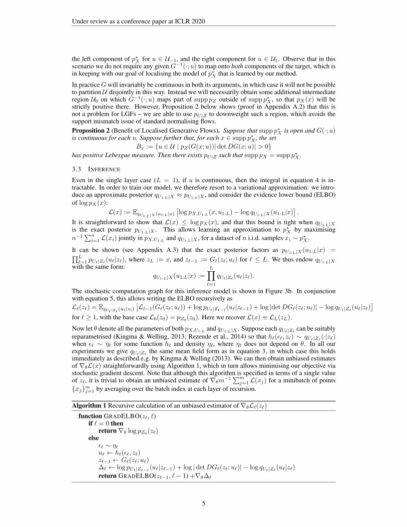
Algorithm 1 Recursive calculation of an unbiased estimator of∇θL`(z`)function GRADELBO(z`, `)

if ` = 0 thenreturn ∇θ log pZ0(z`)

elseε` ∼ η`u` ← h`(ε`, z`)z`−1 ← G`(z`;u`)∆` ← log pU`|Z`−1

(u`|z`−1) + log |detDG`(z`;u`)| − log qU`|Z`(u`|z`)return GRADELBO(z`−1, `− 1) +∇θ∆`

5


3.3.1 PERFORMANCE

A major reason for the popularity of normalising flows is the tractability of their exact log likeli-hoods. In contrast, the variational scheme described here can produce at best an approximation tothis value, which we might expect reduces performance of the final density estimator learned. More-over, particularly when the number of layers L is large, it might seem that the variance of gradientestimators obtained from Algorithm 1 would be impractically high.

However, in practice we have not found either of these problems to be a significant limitation, as ourexperimental results in Section 5 show. Empirically we find improved performance over standardflows even when using the ELBO as our training objective. We also find that importance samplingis sufficient for obtaining good, low-variance (if slightly negatively biased) estimates of log pX(x)(Rezende et al., 2014, Appendix E) at test time, although we do note that the stochasticity here canlead to small artefacts like the occasional white spots visible above in our 2-D experiments.

We similarly do not find that the variance of Algorithm 1 grows intractably when we use a largenumber of layers L, and in practice we are able to train models having the same depth as popularnormalising flows. We conjecture that this occurs because, as the number of stacked bijections inour generative process grows, the complexity required of each individual bijection to map pZ top?X naturally decreases. We therefore have reason to think that, as L becomes large, learning eachqU`|Z` will become easier, so that the variance at each layer will decrease and the overall variancewill remain fairly stable.

3.4 CHOICE OF INDEXED BIJECTION FAMILY

We now consider the choice of G, for which there are many possibilities. In our experiments, whichall take Z = Rd, we focus on the simple case of

G(x;u) = exp(s(u))� g(x) + t(u), (6)where s, t : U → Z are unrestricted mappings, g : X → Z is a bijection, and� denotes elementwisemultiplication. In this case log |detDG(x;u)| = log |detDg(x)|+

∑di=1[s(u)]i, where [s(u)]i is

the ith component of s(u). This has the advantage of working out-of-the-box with all pre-existingnormalising flow methods for which a tractable Jacobian of g is available. We provide alternativesuggestions to this construction in Appendix C.

Equation 6 also has an appealing similarity with the common practice of applying affine transforma-tions between flow steps for normalisation purposes, which has been found empirically to improvestability, convergence time, and overall performance (Dinh et al., 2016; Papamakarios et al., 2017;Kingma & Dhariwal, 2018). In prior work, s and t have been simple parameters that are learnedeither directly as part of the model, or updated according to running batch statistics. Our approachmay be understood as a generalisation of these techniques.

4 RELATED WORK

4.1 DISCRETE MIXTURE METHODS

Several density models exist that involve discrete mixtures of normalising flows. A closely-relatedapproach to ours is RAD (Dinh et al., 2019), which is a special case of our model when L = 1, uis discrete, and X is partitioned disjointly. In the context of Monte Carlo estimation, Duan (2019)proposes a similar model to RAD that does not use partitioning. Ziegler & Rush (2019) introduce anormalising flow model for sequences with an additional latent variable indicating sequence length.More generally, our method may be considered an addition to the class of deep mixture models(Tang et al., 2012; Van den Oord & Schrauwen, 2014), with our use of continuous mixing vari-ables designed to reduce the computational difficulties that arise when stacking discrete mixtureshierarchically – we refer the reader to Appendix B for more details on this.

4.2 METHODS COMBINING VARIATIONAL INFERENCE AND NORMALISING FLOWS

There is also a large class of methods which use normalising flows to improve the inference proce-dure in variational inference (van den Berg et al., 2018; Kingma et al., 2016; Rezende & Mohamed,2015), although flows are not typically present in the generative process here. This approach can bedescribed as using normalising flows to improve variational inference, which contrasts our goal ofusing variational inference to improve normalising flows.

6


However, there are indeed some methods augmenting normalising flows with variational inference,but in all cases below the variational structure is not stacked to obtain extra expressiveness. Ho et al.(2019) use a variational scheme to improve upon the standard dequantisation method for deep gener-ative modelling of images (Theis et al., 2015); this approach is orthogonal to ours and could indeedbe used alongside LGFs. Gritsenko et al. (2019) also generalise normalising flows using variationalmethods, but they incorporate the extra latent noise into the model in a much more restrictive way.Das et al. (2019) only learn a low-dimensional prior over the noise space variationally.

4.3 STACKED VARIATIONAL METHODS

Finally, we can contrast our approach with purely variational methods which are not flow-based,but still involve some type of stacking architecture. The main difference between these methodsand LGFs is that the bijections we use provide us with a generative model with far more structure,which allows us to build appropriate inference models more easily. Contrast this with, for example,Rezende et al. (2014), in which the layers are independently inferred, or Sønderby et al. (2016),which requires a complicated parameter-sharing scheme to reliably perform inference. A single-layer instance of our model also shares some similarity with the fully-unsupervised case in Maaløeet al. (2016), but the generative process there conditions the auxiliary variable on the data.

5 EXPERIMENTS

We evaluated the performance of LGFs on several problems of varying difficulty, including synthetic2-D data, several UCI datasets, and two image datasets. We describe the results of the UCI and imagedatasets here; Appendix D.2 contains the details of our 2-D experiments.

In each case, we compared a baseline flow to its extension as an LGF model with roughly the samenumber of parameters. We obtained each LGF by inserting a mixing variable U` between everycomponent layer of the baseline flow. For example, we inserted a U` after each autoregressivelayer in MAF (Papamakarios et al., 2017), and after each affine coupling layer in RealNVP (Dinhet al., 2016). In all cases we obtained pU`|Z`−1

, qU`|Z` , s`, and t` as described in Appendix D.1.We inserted batch normalisation (Ioffe & Szegedy, 2015) between flow steps for the baselines assuggested by Dinh et al. (2016), but omit it for the LGFs, since our choice of bijection family is ageneralisation of batch normalisation as described in Subsection 3.4.

We trained our models to maximise either the log-likelihood (for the baselines) or the ELBO (forthe LGFs) using the ADAM optimiser (Kingma & Ba, 2014) with default hyperparameters andno weight decay. For the UCI and image experiments we stopped training after 30 epochs of novalidation improvement for the UCI experiments, and after 50 epochs for the image experiments.Both validation and test performance were evaluated using the exact log-likelihood for the baseline,and the standard importance sampling estimator of the average log-likelihood (Rezende et al., 2014,Appendix E) for LGFs. For validation we used 5 importance samples for the UCI datasets and 10for the image datasets, while for testing we used 1000 importance samples in all cases. Our code isavailable at https://github.com/anonsubmission974/lgf.

5.1 UCI DATASETS

We tested the performance of LGFs on the POWER, GAS, HEPMASS, and MINIBOONE datasetsfrom the UCI repository (Bache & Lichman, 2013). We preprocessed these datasets identically toPapamakarios et al. (2017), and use the same train/validation/test splits. For all models we used abatch size of 1000 and a learning rate of 10−3. These constitute a factor of 10 increase over thevalues used by Papamakarios et al. (2017) and were chosen to decrease training time. Our baselineresults differ slightly from Papamakarios et al. (2017), which may be as a result of this change.

We focused on MAF as our baseline normalising flow because of its improved performance overalternatives such as RealNVP for general-purpose density estimation (Papamakarios et al., 2017).A given MAF model is defined by how many autoregressive layers it uses as well as the sizes ofthe autoregressive networks at each layer. For an LGF-MAF, we must additionally define the neuralnetworks used in the generative and inference process, for which we use multi-layer perceptrons(MLPs). We considered a variety of choices of hyperparameters for MAF and LGF-MAF. Eachinstance of LGF-MAF had a corresponding MAF configuration, but in order to compensate for theparameters introduced by our additional neural networks, we also considered deeper and wider MAFmodels. For each LGF-MAF, the dimensionality of u` was roughly a quarter of that of the data. Fullhyperparameter details are given in Appendix D.3. For three random seeds, we trained models using

7

https://github.com/anonsubmission974/lgf


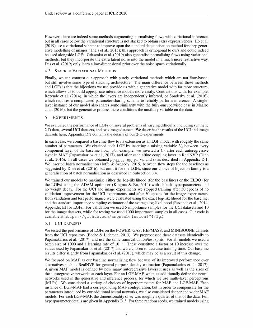
Table 1: Average plus/minus standard error of the best test-set log-likelihood.

POWER GAS HEPMASS MINIBOONE

MAF 0.19± 0.02 9.23± 0.07 −18.33± 0.10 −10.98± 0.03LGF-MAF 0.48± 0.01 12.02± 0.10 −16.63± 0.09 −9.93± 0.04

every hyperparameter configuration, and then chose the best-performing model across all parameterconfigurations using validation performance. Table 1 shows the resulting test-set log-likelihoodsaveraged across the different seeds. It is clear that LGF-MAFs yield improved results in this case.

5.2 IMAGE DATASETS

We also considered LGFs applied to the Fashion-MNIST (Xiao et al., 2017) and CIFAR-10(Krizhevsky et al., 2009) datasets. In both cases we applied the dequantisation scheme of Theiset al. (2015) beforehand, and trained all models with a learning rate of 10−4 and a batch size of 100.

We took our baseline to be a RealNVP with the same architecture used by Dinh et al. (2016) for theirCIFAR-10 experiments. In particular, we used 10 affine coupling layers with the correspondingalternating channelwise and checkerboard masks. Each coupling layer used a ResNet (He et al.,2016a;b) consisting of 8 residual blocks of 64 channels (denoted 8 × 64 for brevity). We alsoreplicated their multi-scale architecture, squeezing the channel dimension after the first 3 couplinglayers, and splitting off half the dimensions after the first 6. This model had 5.94M parametersfor Fashion-MNIST and 6.01M parameters for CIFAR-10. For completeness, we also consider aRealNVP model with coupler networks of size 4× 64 to match those used below in LGF-RealNVP.This model had 2.99M and 3.05M parameters for Fashion-MNIST and CIFAR-10 respectively.

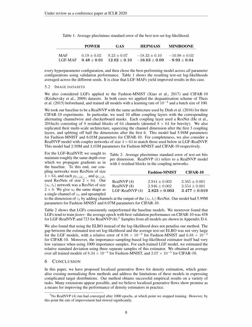
Table 2: Average plus/minus standard error of test-set bitsper dimension. RealNVP (k) refers to a RealNVP modelwith k residual blocks in the coupling networks.

Fashion-MNIST CIFAR-10

RealNVP (4) 2.944± 0.003 3.565± 0.001RealNVP (8) 2.946± 0.002 3.554± 0.001LGF-RealNVP (4) 2.823± 0.003 3.477± 0.019

For the LGF-RealNVP, we sought tomaintain roughly the same depth overwhich we propagate gradients as inthe baseline. To this end, our cou-pling networks were ResNets of size4× 64, and each pU`|Z`−1

and qU`|Z`used ResNets of size 2 × 64. Our(s`, t`) network was a ResNet of size2 × 8. We give u` the same shape asa single channel of z`, and upsampledto the dimension of z` by adding channels at the output of the (s`, t`) ResNet. Our model had 5.99Mparameters for Fashion-MNIST and 6.07M parameters for CIFAR-10.

Table 2 shows that LGFs consistently outperformed the baseline models. We moreover found thatLGFs tend to train faster: the average epoch with best validation performance on CIFAR-10 was 458for LGF-RealNVP, and 723 for RealNVP (8).5 Samples from all models are shown in Appendix D.4.

We also found that using the ELBO instead of the log-likelihood does not penalise our method. Thegap between the estimated test-set log-likelihood and the average test-set ELBO was not very largefor the LGF models, with a relative error of 8.98 × 10−3 for Fashion-MNIST and 6.88 × 10−3

for CIFAR-10. Moreover, the importance-sampling-based log-likelihood estimator itself had verylow variance when using 1000 importance samples. For each trained LGF model, we estimated therelative standard deviation using three separate samples of this estimator. We obtained an averageover all trained models of 8.34× 10−4 for Fashion-MNIST, and 2.07× 10−5 for CIFAR-10.

6 CONCLUSION

In this paper, we have proposed localised generative flows for density estimation, which gener-alise existing normalising flow methods and address the limitations of these models in expressingcomplicated target distributions. Our method obtains successful empirical results on a variety oftasks. Many extensions appear possible, and we believe localised generative flows show promise asa means for improving the performance of density estimators in practice.

5No RealNVP (4) run had converged after 1000 epochs, at which point we stopped training. However, bythis point the rate of improvement had slowed significantly.

8


REFERENCES

Martin Arjovsky, Soumith Chintala, and Leon Bottou. Wasserstein generative adversarial networks.In International conference on machine learning, pp. 214–223, 2017.

K. Bache and M. Lichman. UCI machine learning repository, 2013. URL http://archive.ics.uci.edu/ml.

Jens Behrmann, Will Grathwohl, Ricky TQ Chen, David Duvenaud, and Joern-Henrik Jacobsen.Invertible residual networks. In International Conference on Machine Learning, pp. 573–582,2019.

Patrick Billingsley. Probability and measure. John Wiley & Sons, 2008.

Christopher M Bishop. Pattern recognition and machine learning. Springer, 2006.

Joseph T Chang and David Pollard. Conditioning as disintegration. Statistica Neerlandica, 51(3):287–317, 1997.

Hari Prasanna Das, Pieter Abbeel, and Costas J Spanos. Dimensionality reduction flows. arXivpreprint arXiv:1908.01686, 2019.

Laurent Dinh, David Krueger, and Yoshua Bengio. Nice: Non-linear independent components esti-mation. arXiv preprint arXiv:1410.8516, 2014.

Laurent Dinh, Jascha Sohl-Dickstein, and Samy Bengio. Density estimation using real NVP. arXivpreprint arXiv:1605.08803, 2016.

Laurent Dinh, Jascha Sohl-Dickstein, Razvan Pascanu, and Hugo Larochelle. A RAD approach todeep mixture models. arXiv preprint arXiv:1903.07714, 2019.

Leo L Duan. Transport Monte Carlo. arXiv preprint arXiv:1907.10448, 2019.

Mathieu Germain, Karol Gregor, Iain Murray, and Hugo Larochelle. Made: Masked autoencoder fordistribution estimation. In International Conference on Machine Learning, pp. 881–889, 2015.

Will Grathwohl, Ricky TQ Chen, Jesse Betterncourt, Ilya Sutskever, and David Duvenaud.FFJORD: Free-form continuous dynamics for scalable reversible generative models. arXivpreprint arXiv:1810.01367, 2018.

Alexey A Gritsenko, Jasper Snoek, and Tim Salimans. On the relationship between normalisingflows and variational- and denoising autoencoders. In DGS@ICLR, 2019.

Kaiming He, Xiangyu Zhang, Shaoqing Ren, and Jian Sun. Deep residual learning for image recog-nition. In Proceedings of the IEEE conference on computer vision and pattern recognition, pp.770–778, 2016a.

Kaiming He, Xiangyu Zhang, Shaoqing Ren, and Jian Sun. Identity mappings in deep residualnetworks. In European conference on computer vision, pp. 630–645. Springer, 2016b.

Jonathan Ho, Xi Chen, Aravind Srinivas, Yan Duan, and Pieter Abbeel. Flow++: Improving flow-based generative models with variational dequantization and architecture design. In InternationalConference on Machine Learning, pp. 2722–2730, 2019.

Chin-Wei Huang, David Krueger, Alexandre Lacoste, and Aaron Courville. Neural autoregressiveflows. In International Conference on Machine Learning, pp. 2083–2092, 2018.

Sergey Ioffe and Christian Szegedy. Batch normalization: Accelerating deep network training byreducing internal covariate shift. In International Conference on Machine Learning, pp. 448–456,2015.

Priyank Jaini, Kira A Selby, and Yaoliang Yu. Sum-of-squares polynomial flow. In InternationalConference on Machine Learning, pp. 3009–3018, 2019.

Diederik P Kingma and Jimmy Ba. Adam: A method for stochastic optimization. arXiv preprintarXiv:1412.6980, 2014.

9

http://archive.ics.uci.edu/ml

http://archive.ics.uci.edu/ml


Durk P Kingma and Prafulla Dhariwal. Glow: Generative flow with invertible 1x1 convolutions. InAdvances in Neural Information Processing Systems, pp. 10215–10224, 2018.

Durk P Kingma and Max Welling. Auto-encoding variational Bayes. arXiv preprintarXiv:1312.6114, 2013.

Durk P Kingma, Tim Salimans, Rafal Jozefowicz, Xi Chen, Ilya Sutskever, and Max Welling. Im-proved variational inference with inverse autoregressive flow. In Advances in neural informationprocessing systems, pp. 4743–4751, 2016.

Alex Krizhevsky, Geoffrey Hinton, et al. Learning multiple layers of features from tiny images.Technical report, Citeseer, 2009.

Lars Maaløe, Casper Kaae Sønderby, Søren Kaae Sønderby, and Ole Winther. Auxiliary deep gen-erative models. In International Conference on Machine Learning, pp. 1445–1453, 2016.

Chris J Maddison, Andriy Mnih, and Yee Whye Teh. The concrete distribution: A continuousrelaxation of discrete random variables. arXiv preprint arXiv:1611.00712, 2016.

George Papamakarios, Theo Pavlakou, and Iain Murray. Masked autoregressive flow for densityestimation. In Advances in Neural Information Processing Systems, pp. 2338–2347, 2017.

Gabriel Peyre, Marco Cuturi, et al. Computational optimal transport. Foundations and Trends R© inMachine Learning, 11(5-6):355–607, 2019.

Danilo Rezende and Shakir Mohamed. Variational inference with normalizing flows. In Interna-tional Conference on Machine Learning, pp. 1530–1538, 2015.

Danilo Jimenez Rezende, Shakir Mohamed, and Daan Wierstra. Stochastic backpropagation and ap-proximate inference in deep generative models. In International Conference on Machine Learn-ing, pp. 1278–1286, 2014.

Casper Kaae Sønderby, Tapani Raiko, Lars Maaløe, Søren Kaae Sønderby, and Ole Winther. Laddervariational autoencoders. In Advances in neural information processing systems, pp. 3738–3746,2016.

Yichuan Tang, Ruslan Salakhutdinov, and Geoffrey Hinton. Deep mixtures of factor analysers.In Proceedings of the 29th International Conference on International Conference on MachineLearning, pp. 1123–1130. Omnipress, 2012.

Lucas Theis, Aaron van den Oord, and Matthias Bethge. A note on the evaluation of generativemodels. arXiv preprint arXiv:1511.01844, 2015.

Rianne van den Berg, Leonard Hasenclever, Jakub M Tomczak, and Max Welling. Sylvester normal-izing flows for variational inference. In UAI 2018: The Conference on Uncertainty in ArtificialIntelligence (UAI), pp. 393–402, 2018.

Aaron Van den Oord and Benjamin Schrauwen. Factoring variations in natural images with deepGaussian mixture models. In Advances in Neural Information Processing Systems, pp. 3518–3526, 2014.

Han Xiao, Kashif Rasul, and Roland Vollgraf. Fashion-mnist: a novel image dataset for benchmark-ing machine learning algorithms. arXiv preprint arXiv:1708.07747, 2017.

Zachary Ziegler and Alexander Rush. Latent normalizing flows for discrete sequences. In Interna-tional Conference on Machine Learning, pp. 7673–7682, 2019.

10


A ADDITIONAL PROOFS

A.1 PROOF OF PROPOSITION 1 (SEE PAGE 2)

Proposition 1 (Limitations of Normalising Flows). Suppose each gθ is a homeomorphism anddetDgθ(x) 6= 0 for all θ and x. If the prior pZ has a support that is not homeomorphic to p∗X ,then no choice of θ will yield a normalising flow model that matches p∗X exactly.

Proof. For any choice of θ, let pθX(x) be the normalising flow model produced by pZ and gθ, i.e.pθX(x) = pZ(gθ(x))|detDgθ(x)|.

We can bound the total variation distance dTV between pθX and p?X by

dTV(p?X , pθX) ≥

∣∣∣∣∣∫supp p?X

p?X(x)dx−∫supp p?X

pθX(x)dx

∣∣∣∣∣=

∣∣∣∣∣1−∫supp p?X∩supp pθX

pθX(x)dx

∣∣∣∣∣ .Observe that this is strictly positive unless supp p?X = supp pθX (up to a set of pθX -probability 0). Butsince gθ is a homeomorphism, this is not possible. Hence dTV(p?X , p

θX) > 0, so that p?X 6= pθX .

A.2 PROOF OF PROPOSITION 2 (SEE PAGE 5)

Proposition 2 (Benefit of Localised Generative Flows). Suppose that supp p∗X is open and G(·;u)is continuous for each u. Suppose further that, for each x ∈ supp p∗X , the set

Bx := {u ∈ U | pZ(G(x;u))|detDG(x;u)| > 0}has positive Lebesgue measure. Then there exists pU |Z such that supp pX = supp p∗X .

Proof. Take pU to be any positive density. DefineAu := G(supp p∗X ;u).

Observe that eachAu has positive Lebesgue measure, since it is the continuous injective image of anopen set. Thus, for each u, we can choose pZ|U (·|u) to be any positive density on Au. This allowsus to define

pU |Z(u|z) :=pZ|U (z|u)pU (u)∫pZ|U (z|u′)pU (u′)du′

.

We claim this construction gives supp pX = supp p∗X . First suppose x ∈ supp p∗X . For each u,observe that pZ|U (G(x;u)|u) > 0 by the definition of Au, and hence pU |Z(u|G(x;u)) > 0 sincepU is positive. Consequently,

pX(x) ≥∫Bx

pZ(G(x;u))pU |Z(u|G(x;u))|detDG(x;u)| du > 0

since the integrand is strictly positive on Bx, which has positive measure.

Now suppose x 6∈ supp p∗X . For each u, since pZ|U (·|u) is supported on Au, we must havepZ|U (G(x;u)|u) = 0, and hence pU |Z(u|G(x;u)) = 0. From this it follows directly thatpX(x) = 0, i.e. x 6∈ supp pX .

A.3 CORRECTNESS OF POSTERIOR FACTORISATION

We want to prove that the exact posterior factorises according to

pU1:L|X(u1:L|x) =

L∏`=1

pU`|Z`(u`|z`), (7)

where ZL ≡ X , zL ≡ x, and z`−1 := G`(z`;u`) for ` ≤ L. It is convenient to introduce the indexnotation U>` ≡ U`+1:L. First note that we can always write this posterior autoregressively as

pU1:L|X(u1:L|x) =

L∏`=1

pU`|U>`,X(u`|u>`, x). (8)

11


Now, consider the graph of the full generative model shown in Figure 3a. It is clear that all pathsfrom U` to any node in the set H` := {U>`, Z>`} are blocked by Z`, and hence that Z` d-separatesH` from U` (Bishop, 2006). Consequently,

pU`|Z`,U>`,X(u`|z`, u>`, x) ≡ pU`|Z`(u`|z`).

Informally,6 we then have the following for any ` ∈ {1, . . . , L− 1}:

pU`|U>`,X(u`|u>`, x) =

∫pU`,Z`|U>`,X(u`, z`|u>`, x)dz`

=

∫pU`|Z`,U>`,X(u`|z`, u>`, x)pZ`|U>`,X(z`|u>`, x)dz`

=

∫pU`|Z`(u`|z`)δ

(z` −

(G`+1,u`+1

◦ · · · ◦GL,uL)

(x))dz`

= pU`|Z`(u`|(G`+1,u`+1

◦ · · · ◦GL,uL)

(x))

= pU`|Z`(u`|z`)by the definition of z`, where we write G`(·;u) ≡ G`,u(·) to remove any ambiguities when com-posing functions. We can substitute this result into equation 8 to obtain equation 7.

B DISCRETE u

While a discrete u is appealing for its ability to produce exact likelihoods, it also suffers severaldisadvantages that we describe now. First, observe that the choice of the number of discrete valuestaken by u has immediate implications for the number of disconnected components of supp p?Xthat G can separate, which therefore seems to require making fairly concrete assumptions (perhapsimplicitly) about the topology of the target of interest. To mitigate this, we might try taking thenumber of u values to be very large, but then in turn the time required to evaluate equation 4 (nowa sum rather than an integral) necessarily increases. This is particularly true when using a stackedarchitecture, since to evaluate pX(x) with L layers each having K possible u-values takes Θ(KL)complexity. Dinh et al. (2019) propose a model that partitions X so that only one component in eachsummation is nonzero for any given x, which reduces this cost to Θ(L). However, this partitioningmeans that their pX is not continuous as a function of x, which is reported to make the optimisationproblem in equation 2 difficult.

Unlike for continuous u, the ELBO objective is also of limited effectiveness in the discrete case.Since pU`|Z`−1

defines a discrete distribution at each layer, we would need a discrete variationalapproximation qU`|Z` to ensure a well-defined ELBO. However, the parameters of a discrete dis-tribution are not ameanble to the reparametrisation trick, and hence we would expect our gradientestimates of the ELBO to have high variance. As mentioned above, a compromise here might beto use the CONCRETE distribution (Maddison et al., 2016) to approximate a discrete u while stillapply variational methods. We leave exploring this for future work.

C OTHER CHOICES OF INDEXED BIJECTION FAMILY

Other choices of G than our suggestion in Subsection 3.4 are certainly possible. For instance, wehave had preliminary experimental success on small problems by simply taking g to be the identity,in which case the model is greatly simplified by not requiring any Jacobians at all. Alternatively, it isalso frequently possible to modify the architecture of standard choices of g to obtain an appropriateG. For instance, affine coupling layers, a key component of models such as RealNVP (Dinh et al.,2016), make use of neural networks that take as input a subset of the dimensions of x. By concate-nating u to this input, we straightforwardly obtain a family of bijections G(·;u) for each value ofu. This requires more work to implement than our suggested method, but has the advantage of nolonger requiring a choice of s and t. We have again had preliminary empirical success with thisapproach. We leave a more thorough exploration of these alternative possibilites for future work.

6As with our arguments in Subsection 3.1, this could again be made precise using disintegrations (Chang &Pollard, 1997).

12


D FURTHER EXPERIMENTAL DETAILS

D.1 LGF ARCHITECTURE

In addition to the bijections from the baseline flow, an LGF model of the form we consider requiresspecifying pU`|Z`−1

, qU`|Z` , s` and t`. In all our experiments

• pU`|Z`−1(·|z`−1) = Normal

(µp(z`−1), σp(z`−1)2

), where µp and σp were two separate

outputs of the same neural network

• qU`|Z`(·|z`) = Normal(µq(z`), σq(z`)

2), where µq and σq were two separate outputs of

the same neural network

• s` and t` were two separate outputs of the same neural network.

D.2 2-D EXPERIMENTS

To gain intuition about our model, we ran several experiments on the simple 2-D datasets shown inFigure 1 and Figure 4. Specifically, we compared the performance of a baseline MAF against anLGF-MAF. We used MLPs for all networks involved in our model.

For the dataset shown in Figure 1, the baseline MAF had 10 autoregressive layers consisting of4 hidden layers with 50 hidden units. The LGF-MAF had 5 autoregressive layers consisting of 2hidden layers with 10 hidden units. Each u` was a single scalar. The (s`, t`) network consisted of 2hidden layers of 10 hidden units, and both the (µp, σp) and (µq, σq) networks consisted of 4 hiddenlayers of 50 hidden units. In total the baseline MAF had 80080 parameters, while LGF-MAF had80810 parameters. We trained both models for 300 epochs.

We used more parameters for the datasets shown in Figure 4, since these targets have more compli-cated topologies. In particular, the baseline MAF had 20 autoregressive layers, each with the samestructure as before. The LGF-MAF had 5 autoregressive layers, now with 4 hidden layers of 50hidden units. The other networks were the same as before, and each u` was still a scalar. In totalthe baseline MAF had 160160 parameters, while our model had 119910 parameters. We trained allmodels now for 500 epochs.

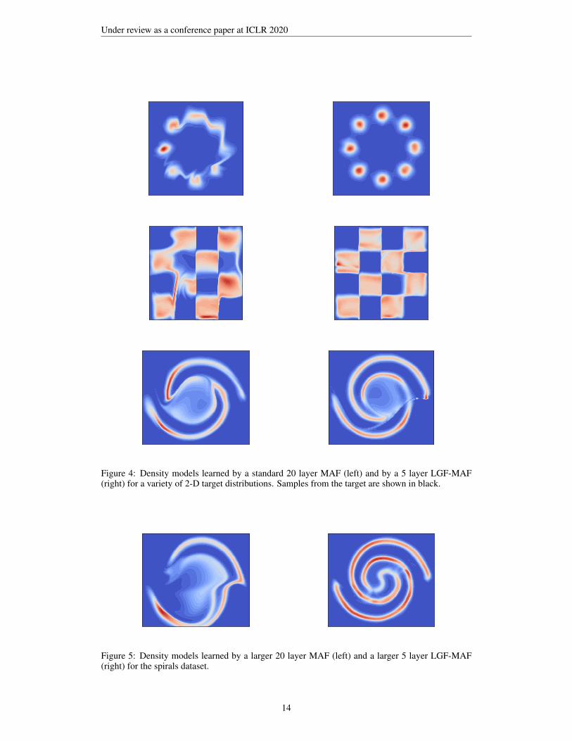
The results of these experiments are shown in Figure 1 and Figure 4. Observe that LGF-MAFconsistently produces a more faithful representation of the target distribution than the baseline. Afailure mode of our approach is exhibited in the spiral dataset, where our model still lacks the powerto fully capture the topology of the target. However, we did not find it difficult to improve on this:by increasing the size of the mean/standard deviation networks to 8 hidden layers of 50 hidden units(and keeping all other parameters fixed), we were able to obtain the result shown in Figure 5. Thismodel had a total of 221910 parameters. For the sake of a fair comparison, we also tried increasingthe complexity of the MAF model, by the size of its autoregressive networks to 8 hidden layers of50 hidden units (obtaining 364160 parameters total). This model diverged after approximately 160epochs. The result after 150 epochs is shown in Figure 5.

D.3 UCI EXPERIMENTS

In Tables 3, 4, and 5, we list the choices of parameters for MAF and LGF-MAF. In all cases, weallowed the base MAF to have more layers and deeper coupler networks to compensate for theadditional parameters added by the additional components of our model. Note that neural networksare listed as size K1 ×K2, where K1 denotes the number of hidden layers and K2 denotes the sizeof the hidden layers. All combinations of parameters were considered; in each case, there were 9configurations for MAF and 8 configurations for LGF-MAF.

Table 3: Parameter configurations for POWER and GAS.

Layers Coupler size u dim p, q size s, t size

MAF 5, 10, 20 2× 100, 2× 200, 2× 400 - - -LGF-MAF 5, 10 2× 128 2 2× 100, 2× 200 2× 128

13


Figure 4: Density models learned by a standard 20 layer MAF (left) and by a 5 layer LGF-MAF(right) for a variety of 2-D target distributions. Samples from the target are shown in black.

Figure 5: Density models learned by a larger 20 layer MAF (left) and a larger 5 layer LGF-MAF(right) for the spirals dataset.

14


Table 4: Parameter configurations for HEPMASS


MAF 5, 10, 20 2× 128, 2× 512, 2× 1024 - - -LGF-MAF 5, 10 2× 128 5 2× 128, 2× 512 2× 128

Table 5: Parameter configurations for MINIBOONE


MAF 5, 10, 20 2× 128, 2× 512, 2× 1024 - - -LGF-MAF 5, 10 2× 128 10 2× 128, 2× 512 2× 128

D.4 IMAGE EXPERIMENTS

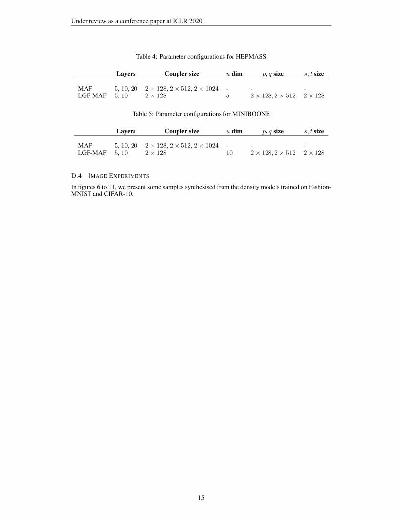
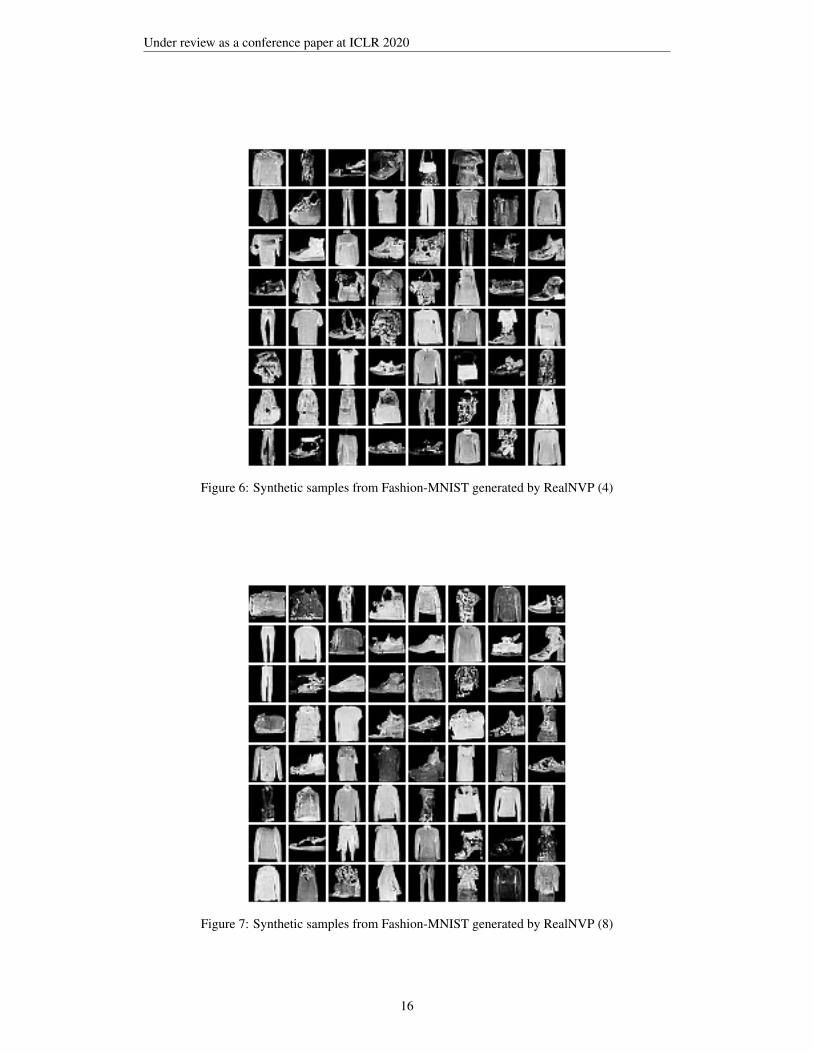
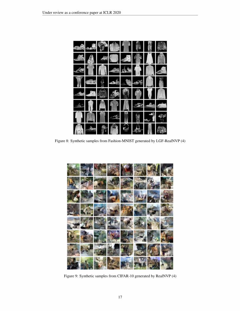
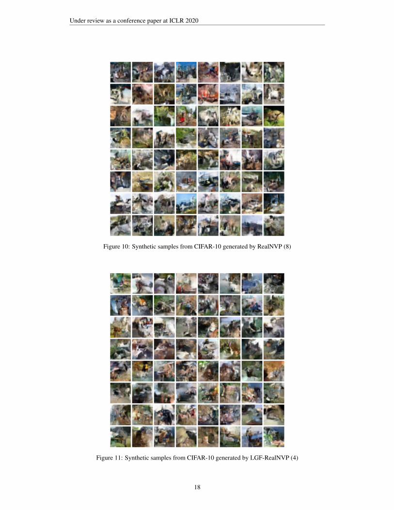
In figures 6 to 11, we present some samples synthesised from the density models trained on Fashion-MNIST and CIFAR-10.

15


Figure 6: Synthetic samples from Fashion-MNIST generated by RealNVP (4)

Figure 7: Synthetic samples from Fashion-MNIST generated by RealNVP (8)

16


Figure 8: Synthetic samples from Fashion-MNIST generated by LGF-RealNVP (4)

Figure 9: Synthetic samples from CIFAR-10 generated by RealNVP (4)

17


Figure 10: Synthetic samples from CIFAR-10 generated by RealNVP (8)

Figure 11: Synthetic samples from CIFAR-10 generated by LGF-RealNVP (4)

18

Documents

LOCALISED GENERATIVE FLOWS - OpenReview