Local Receptive Field Constrained Deep Networks

Diana Turcsanya,∗, Andrzej Bargielab, Tomas Maulc

aSchool of Computer Science, The University of Nottingham, Nottingham, NG81BB, United KingdombInfohub Ltd, Nottingham Science and Technology Park, Nottingham, NG72QJ, United Kingdom

cSchool of Computer Science, The University of Nottingham Malaysia Campus, Semenyih, 43500, Malaysia

Abstract

Automatic extraction of distinctive features from a visual information stream is challenging due to thelarge amount of information contained in most image data. In recent years deep neural networks (DNNs)have gained outstanding popularity for solving visual information processing tasks. This study reportsnovel contributions, including a new DNN architecture and training method, which increase the fidelity ofDNN-based representations to encodings extracted by visual processing neurons. Our local receptive fieldconstrained DNNs (LRF-DNNs) are pre-trained with a modified restricted Boltzmann machine, the LRF-RBM, which utilizes biologically inspired Gaussian receptive field constraints to encourage the emergence oflocal features. Moreover, we propose a method for concurrently finding advantageous receptive field centers,while training the LRF-RBM. By utilizing LRF-RBMs with gradually increasing receptive field sizes oneach layer, our LRF-DNN learns features of increasing complexity and demonstrates hierarchical part-basedcompositionality. We show superior face completion and reconstruction results on the challenging LFW facedataset.

Keywords: visual information encoding, local receptive field learning, feature hub, deep autoencoderneural network, self-adaptive structure, face completion

1. Introduction

The highly accurate vision of humans and other biological systems has long been studied in neuroscienceand biology. This great effort has brought about important discoveries regarding the morphology andfunctionality of neural cells and networks. However, our knowledge of visual information processing circuitsand the specific roles of cells within the visual pathway is still far from complete.

Designing computational models of these circuits has great importance for improving our understandingof biological visual information processing and hence providing a more informed background for the designof visual data processing units, e.g., retinal implants. Modeling biological information processing withinthe visual pathway is not only important for neuroscientific and medical research but is a key challenge inInformation Sciences in general, underpinning many areas of machine learning, cognitive science, and intel-ligent systems research. Furthermore, modeling biological vision can provide important practical benefitsfor algorithm design in image processing and computer vision.

Traditional modeling studies have focused on directly implementing functionalities of visual informationprocessing cells and circuits based on our current knowledge, obtained from biological studies, regarding theworkings of the visual system. Nowadays however, with the constant advancement in experimental equip-ment and methodology, this ‘current knowledge’ changes ever so rapidly. Due to incomplete understandingof visual processing mechanisms in biological systems, designing robust computational models of these pro-cesses prompts one to account for uncertainty and unknown details. Flexible probabilistic models, such asdeep belief networks (DBNs) [11], offer great potential for modeling in this uncertain environment.

∗Corresponding authorEmail address: dxt@cs.nott.ac.uk (Diana Turcsany)URL: http://www.cs.nott.ac.uk/~dxt/ (Diana Turcsany)

Preprint submitted to Information Sciences February 9, 2016

1.1. Deep Networks

Many areas of visual information processing research, such as computer vision, has traditionally reliedon the hand-crafted SIFT [27], GA-SIFT [25] or similar local feature detectors [3, 34], often followed by bag-of-words type quantization techniques [40, 43, 46], for the successful design of accurate systems [2, 26, 50].Recently however, deep learning has emerged as a popular research area within machine learning, whichfocuses on automatically learning a hierarchy of relevant features directly from input data instead of applyinggeneric, hand-crafted feature detectors. Such feature hierarchies can be well captured by multi-layer networkmodels, such as deep belief networks, deep neural networks (DNNs) or convolutional networks (CNNs) [21].

To learn a multi-layer generative model of the data where each higher layer corresponds to a moreabstract representation of information, Hinton et al. [11] train a DBN, first layer by layer, using restrictedBoltzmann machines (RBMs) [41]. The network parameters learned during this unsupervised pre-trainingphase can subsequently be fine-tuned in, e.g., a supervised manner using backpropagation. Such modelswere shown to be superior to PCA for dimensionality reduction [12]. Since this efficient training method fordeep networks was introduced, deep learning research has gained increased interest resulting in wide-rangingacademic and commercial adoption of deep learning techniques. The potential of DBNs, CNNs, and otherdeep architectures [32, 33, 36] for learning meaningful features, and thereby providing improved models of theinput data, has been demonstrated on object recognition [20, 30, 49], image classification [5, 12, 18, 19, 35],and further visual tasks [9, 13, 16, 31, 51] as well as on problems concerning text [12, 37], speech [7], andaudio data [24, 28] analysis.

Multi-layer network models show structural resemblance to biological visual information processing units.For example, the structure of mammalian retina is inherently multi-layered: the different cell types (i.e.,rods, cones, horizontal cells, bipolar cells, amacrine and ganglion cells) are organized into multiple consec-utive processing layers (i.e., the photoreceptor, outer plexiform and inner plexiform layers) which executeincreasingly more difficult tasks. On a larger scale, visual information processing is implemented by consec-utive areas of the visual pathway (i.e., retina, V1, V2, etc.) through the extraction of increasingly complexrepresentations.

While the focus of deep learning research has not been the exact replication of neural connectivitypatterns in biological systems, DBNs have been shown suitable for modeling biological neural networks ofthe visual pathway on a more abstract level. DBNs have been successfully used for modeling functionalityimplemented by neural structures within the retina [45] and the V1 and V2 areas of the visual cortex [22].Despite this success in neural modeling, primal emphasis has been given to improving the performance ofdeep learning models on visual recognition tasks, rather than increasing the fidelity of such deep architecturesto real neural circuits of the visual pathway.

The aim of this study was to take a step towards filling this gap by proposing deep network structuresthat resemble more closely biological neural networks while retaining their flexibility and great performanceon visual tasks. Exploring such architectures possesses high potential for designing improved computationalmodels of neural structures within the visual pathway.

1.2. Contributions

Increasing the fidelity of representations learned by DBNs and DNNs to encodings extracted by visualprocessing neurons could provide benefits for numerous areas of visual information processing research. Thework reported here focused on increasing the structural similarity of deep network models to neural networksof the visual pathway, which, we argue, represents a key step towards this goal.

Visual neurons in consecutive processing layers typically only receive information from neurons in a localarea of restricted size within the previous layer. The receptive field of a neuron refers to the area of thevisual space in which stimuli can result in neural responses. Receptive fields are highly local in the case ofretinal cells and receptive field size gradually increases from local to more global through different areas ofthe visual cortex. The focus of this paper is the extension of deep neural networks with local receptive fieldsin a way that the training process, the final architecture, and the encoding process by which representationsare calculated closely resemble biological neural networks of the visual pathway.

We start from DBN models [11] and by utilizing our local receptive field constrained RBM (LRF-RBM) [44] during pre-training, we obtain a deep network which more closely resembles biological processing

2

and also provides an improved encoding of image features. Our LRF-RBM training procedure allows forseamless integration of local receptive field constraints into RBMs. We also propose a method for con-currently finding advantageous receptive field placement, while training the LRF-RBM. This enables thenetwork to utilize a non-uniform distribution of feature detectors over the visual space. Our novel contri-butions include:

(i) an adaptation of the contrastive divergence learning (CD) [10] algorithm that introduces local receptivefield constraints for hidden nodes of RBMs,

(ii) a method for automatically identifying locations of high importance within the visual input spaceduring RBM training, and utilizing these locations as receptive field centers to obtain a compact, yetpowerful encoding of visual features,

(iii) also, by using LRF-RBMs with increasing size Gaussian receptive field constraints for pre-trainingeach consecutive DBN layer, we construct a biologically inspired local receptive field constrained DBN(LRF-DBN), where consecutive layers detect features of increasing size and complexity,

(iv) we demonstrate the superior performance of LRF-DBN generative models, compared to DBNs, on facecompletion, a task inspired by processing capabilities of higher areas in the visual cortex [4],

(v) furthermore, we show fine-tuning can be implemented for LRF-DBNs analogously to DBNs, and theresulting local receptive field constrained deep neural networks (LRF-DNNs) outperform traditionalDNNs (fine-tuned DBNs) on dimensionality reduction of face images.

We have chosen biologically inspired Gaussian receptive field constraints to encourage learning of localizedfeatures. These constraints are implemented in forms of Gaussian masks over the weights when written inthe shape of the input image data. The learning is conducted in a way that the learned features will notbe restricted to have Gaussian shape, rather the Gaussian constraints encourage the growth of localizedfeatures versus global ones.

1.3. Overview

In Section 2 our approach to modeling local receptive fields in deep networks is compared to previouswork. Section 3 describes the principles of CD training for RBMs. Sections 4 and 5 introduce a newtraining algorithm for DNNs based on our proposed biologically inspired LRF-RBMs. Description of ourexperimental set-up and dataset is provided in Section 6. Our findings are summarized in Section 7, whileSection 8 concludes our paper.

2. Related Work

Local receptive fields have been modeled in deep learning through convolutional neural networks [5, 13,16, 18, 21, 23, 31]. Although the architecture of CNNs was inspired by the organization of the visual cortex,the prime objective has not been the modeling of biological visual processing. The main emphasis has beenon improving the efficiency of learning in multi-layer networks on visual tasks through the use of convolution,thereby scaling up deep learning algorithms to high dimensional problems.

In contrast with CNNs, having fixed network architecture and hand-crafted receptive field organization,our adaptive network model supports the exploration of problem-specific receptive field organization. Featuredetector placement and connection patterns are learned automatically from data, making it possible toexploit particularities of the task at hand.

In CNNs weights between visible and hidden layers are the same across all image locations making thefeature detection translation invariant. When weights are shared, the same feature detectors operate on eachpart of the image within a layer and the training procedure can therefore utilize convolution operations.Translation invariant feature detection sometimes simplifies the learning task, however spurious detectionscan often arise and in some visual recognition tasks translation invariance may not be advantageous. Inseveral cases image data have strong priors on where in the visual space certain feature types are located(e.g., landmarks tend to capture sky in the top area of the image, and in portraits, eyes are located abovethe mouth). In such cases, keeping the feature detection translation invariant throws away important

3

(a) LRF-RBM model

10 20

10

20

30

10 20 10 20 10 20

(b) Receptive field maps on LFW (c) LRF-RBM features

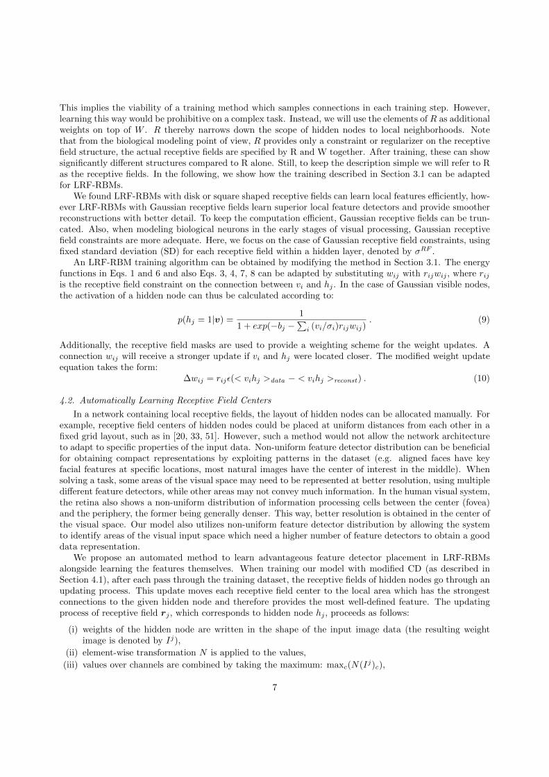
Figure 1: LRF-RBM learning on face images. (a) LRF-RBM model schematic, showing an input image in the visible layer Vand local feature detector receptive fields (blue cones) in the hidden layer H with feature hubs around the eyes and mouth. (b)Receptive field maps of 4000 hidden node LRF-RBMs run with different learning parameters. Automatically learned featuredetector receptive fields are combined to show areas attracting more detectors. Darker red areas indicate higher feature density.Feature hubs emerged around average eye and mouth locations at pixels (9, 15), (20, 15), and (15, 30). (c) Distinctive lookingdetectors located in feature hubs in a 4000 hidden node LRF-RBM. From top to bottom row: Automatically learned detectorsof the persons’ right eye, left eye, nose and mouth can be seen. The second map in (b) belongs to the LRF-RBM whichgenerated the local features in (c).

information particular to the given dataset and task. This can be detrimental for performance due to theresulting false detections, for example, when face recognition is conducted in aligned images the mouthalways appears in the same area, therefore a positive detection of mouth elsewhere will be false.

In contrast, our LRF-RBM is capable of learning the most relevant feature detectors at any one imagelocation. In this model, hidden nodes can only receive input from visible nodes which fall within their localreceptive field, the shape of which is controlled by a Gaussian constraint. Some deep architectures havebeen proposed where local receptive fields are used without weight-sharing, however these systems typicallyapply a fixed grid layout for their rectangular receptive fields [20, 33, 51]. Coates and Ng [6] propose toselect receptive fields for higher layer nodes by grouping together similar features from the previous layer,which can be useful for non-image data.

As opposed to these methods, the receptive field location of our hidden nodes are learned concurrentlywith learning the features themselves. Hidden nodes of an LRF-RBM move around the visual space duringtraining to find the best location for their Gaussian receptive field center.

It is often the case for visual data that some image regions express higher variability within the input, withmultiple distinctive features being present, while other areas are quasi-uniform, therefore less interesting.By letting the detectors move to locations of interest, “feature hubs” (i.e. areas densely covered by featuredetectors) can emerge in image regions where the training data have high variation, while more uniformareas will attract fewer detectors. This way, the structure of our network is morphing throughout thetraining procedure. This self-adaptation results in a network architecture which is capable of extractingcompact representation of visual information, enables very quick query time and by combining local featuresas building blocks, the network is strong at reconstructing previously unseen images. A diagram illustratingthe receptive field learning on face images is shown in Fig. 1(a), together with receptive field distributions ofour trained models in Fig. 1(b), and local features in Fig. 1(c). Figure 2 illustrates the result of LRF-RBMtraining on handwritten digit data by showing the spatial distributions of the most distinctive features perdigit.

It is important to note non-uniform distribution of feature detectors is also utilized in biological neuralnetworks: the structural organization of the retinal network shows a distinct difference between the center

4

10 20

10

20

10 20

10

20

10 20

10

20

10 20

10

20

10 20

10

20

10 20

10

20

10 20

10

20

10 20

10

20

10 20

10

20

10 20

10

20

Figure 2: LRF-RBM receptive field maps learned on the MNIST digit dataset. Top row: Example images of digits are shownfrom 0 to 9. Bottom row: For each digit class, a heat map shows locations of detectors which most selectively fire on imagesof the given digit.

and periphery of the visual space. The density of ganglion cells is highest in the center (fovea) and thesemidget ganglion cells have a very small receptive field. On the other hand, the periphery contains ganglioncells which connect to multiple bipolar cells and thus have large receptive fields [17, 29, 47]. This non-uniformorganization provides high resolution vision in the center and much lower resolution in the periphery.

3. Restricted Boltzmann Machines

The first, unsupervised pre-training phase of Hinton et al. [11]’s DBN training utilizes RBMs for learningeach layer of the representation. The energy-based RBM models consist of a visible and a hidden layer,where connections are only present between visible and hidden nodes but not within a layer. Thanks to thisrestriction, RBMs are bi-partite graphs and therefore are quick to train due to the conditional independenceof hidden nodes given visible nodes and vice versa. This efficiency in training has resulted in widespreadapplication of RBMs within machine learning [9, 12, 15, 28, 30, 33, 36, 38, 39, 42, 48]. In visual recognitiontasks visible nodes usually correspond to visual input coordinates (pixel locations), while hidden nodesrepresent image feature detectors and can thus be seen as models of neurons in the visual pathway.

First we will discuss how RBMs with binary visible and hidden nodes are trained, then show how Gaussianvisible nodes can be used to model continuous valued data (for more details see [10, 11, 30]). Subsequently,we will introduce our LRF-RBM model together with our algorithm for automatically identifying receptivefield centers.

3.1. Contrastive Divergence Learning

The probability of a configuration (state) of visible and hidden nodes (v,h) can be calculated using theenergy function of the RBM, which, in the case of binary visible and hidden nodes, takes the form:

E(v,h) = −aTv − bTh− hTWv , (1)

where W ∈ Rn×m is the weight matrix describing the symmetric connections between visible and hiddennodes, while a and b are the biases of the visible and hidden nodes respectively. The probability of aconfiguration is then given by:

p(v,h) =e−E(v,h)∑η,µ e

−E(η,µ). (2)

Learning aims at reducing the energy (increasing the log probability) of the training data by altering theweights and biases. An efficient training method for RBMs which broadly approximates the gradient of thelog probability of the training data, is the single-step version (CD1) of contrastive divergence learning [10].Each step of CD1 training corresponds to one step of alternating Gibbs sampling. First (i) the visible statesare initialized to a training example, then (ii) hidden states can be sampled in parallel (due to the conditionalindependence of hidden nodes given visible nodes), according to:

p(hj = 1|v) =1

1 + exp(−bj −∑

i viwij), (3)

5

followed by (iii) the reconstruction phase where visible states are sampled using:

p(vi = 1|h) =1

1 + exp(−ai −∑

j hjwij), (4)

finally (iv) the weights are updated according to:

∆wij = ε(< vihj >data − < vihj >reconst) , (5)

where ε is the learning rate, and the correlation between the activations of vi and hj measured after (ii)gives < vihj >data , while the correlation after the reconstruction phase (iii) determines < vihj >reconst . Asimilar rule is applied to the biases. In order to obtain an improved model, the sampling stage in each stepcan be continued for more iterations resulting in a general form of the CD algorithm: CDn, where n is thenumber of alternating Gibbs sampling iterations.

RBMs with Gaussian visible nodes. While RBMs with binary visible nodes are generally easier to train thanRBMs with Gaussian visible nodes, the latter can learn better models of continuous valued data, such asthe face images we studied. In the case of Gaussian visible nodes the energy function changes to:

E(v,h) =∑i

(vi − ai)2

2σ2i

−∑j

bjhj −∑i,j

viσihjwij , (6)

where σi is the standard deviation corresponding to visible node vi. The probability of hidden node activationbecomes:

p(hj = 1|v) =1

1 + exp(−bj −∑

i (vi/σi)wij), (7)

and the expected value of a visible node (i.e., the reconstructed value) is given by:

< vi >reconst= ai + σi∑j

hjwij . (8)

A more detailed description of RBM training principles is provided by [11].

4. Local Receptive Field Constrained RBMs (LRF-RBMs)

4.1. Training with Local Receptive Fields

Visual information processing neurons in early stages of the visual pathway typically only receive inputfrom neurons within a small localized area of the previous processing layer. The area of the photoreceptorlayer in which stimuli can result in neural responses is called the receptive field of a visual processingneuron. Moving up the layers, the receptive field of neurons gets gradually larger and their structurebecomes increasingly more complex. As an example, the receptive field structure of retinal ganglion cellscan be closely modeled by difference-of-Gaussians (DoGs), while receptive fields of V1 simple cells by Gaborfilters.

In LRF-RBMs receptive field constraints of hidden nodes are applied to outline the area from which thehidden node is most likely to receive input. These constraints are given in the form of receptive field masks(denoted by R) that operate on the RBM weights W . Each mask has a center location which corresponds toa hidden node’s location in visual space. These masks describe the likelihood of a connection being presentbetween a visible and a hidden node given the distance between the visible node and the center of the hiddennode’s receptive field. The likelihood of a connection converges to 0 as the distance goes to infinity, whichmeans visible nodes further away are less likely to have a connection to the given hidden node.

R = [r1, . . . , rm] ∈ [0, 1]n×m, which denotes the collection of receptive field masks of all the hidden nodes,is of the same dimension as W , with rij being the receptive field constraint on the connection between visiblenode vi and hidden node hj . The elements of R represent the likelihood of a given connection being present.

6

This implies the viability of a training method which samples connections in each training step. However,learning this way would be prohibitive on a complex task. Instead, we will use the elements of R as additionalweights on top of W . R thereby narrows down the scope of hidden nodes to local neighborhoods. Notethat from the biological modeling point of view, R provides only a constraint or regularizer on the receptivefield structure, the actual receptive fields are specified by R and W together. After training, these can showsignificantly different structures compared to R alone. Still, to keep the description simple we will refer to Ras the receptive fields. In the following, we show how the training described in Section 3.1 can be adaptedfor LRF-RBMs.

We found LRF-RBMs with disk or square shaped receptive fields can learn local features efficiently, how-ever LRF-RBMs with Gaussian receptive fields learn superior local feature detectors and provide smootherreconstructions with better detail. To keep the computation efficient, Gaussian receptive fields can be trun-cated. Also, when modeling biological neurons in the early stages of visual processing, Gaussian receptivefield constraints are more adequate. Here, we focus on the case of Gaussian receptive field constraints, usingfixed standard deviation (SD) for each receptive field within a hidden layer, denoted by σRF .

An LRF-RBM training algorithm can be obtained by modifying the method in Section 3.1. The energyfunctions in Eqs. 1 and 6 and also Eqs. 3, 4, 7, 8 can be adapted by substituting wij with rijwij , where rijis the receptive field constraint on the connection between vi and hj . In the case of Gaussian visible nodes,the activation of a hidden node can thus be calculated according to:

p(hj = 1|v) =1

1 + exp(−bj −∑

i (vi/σi)rijwij). (9)

Additionally, the receptive field masks are used to provide a weighting scheme for the weight updates. Aconnection wij will receive a stronger update if vi and hj were located closer. The modified weight updateequation takes the form:

∆wij = rijε(< vihj >data − < vihj >reconst) . (10)

4.2. Automatically Learning Receptive Field Centers

In a network containing local receptive fields, the layout of hidden nodes can be allocated manually. Forexample, receptive field centers of hidden nodes could be placed at uniform distances from each other in afixed grid layout, such as in [20, 33, 51]. However, such a method would not allow the network architectureto adapt to specific properties of the input data. Non-uniform feature detector distribution can be beneficialfor obtaining compact representations by exploiting patterns in the dataset (e.g. aligned faces have keyfacial features at specific locations, most natural images have the center of interest in the middle). Whensolving a task, some areas of the visual space may need to be represented at better resolution, using multipledifferent feature detectors, while other areas may not convey much information. In the human visual system,the retina also shows a non-uniform distribution of information processing cells between the center (fovea)and the periphery, the former being generally denser. This way, better resolution is obtained in the center ofthe visual space. Our model also utilizes non-uniform feature detector distribution by allowing the systemto identify areas of the visual input space which need a higher number of feature detectors to obtain a gooddata representation.

We propose an automated method to learn advantageous feature detector placement in LRF-RBMsalongside learning the features themselves. When training our model with modified CD (as described inSection 4.1), after each pass through the training dataset, the receptive fields of hidden nodes go through anupdating process. This update moves each receptive field center to the local area which has the strongestconnections to the given hidden node and therefore provides the most well-defined feature. The updatingprocess of receptive field rj , which corresponds to hidden node hj , proceeds as follows:

(i) weights of the hidden node are written in the shape of the input image data (the resulting weightimage is denoted by Ij),

(ii) element-wise transformation N is applied to the values,

(iii) values over channels are combined by taking the maximum: maxc(N(Ij)c),

7

(iv) subsequently, the image is filtered with a Gaussian filter G(σRF , k) with SD σRF and filter size k,

(v) the location with maximum response is selected as the new center:

(pj , qj) = arg maxrs

[maxc

(N(Ij)c) ∗G(σRF , k)]rs , (11)

(vi) finally, the values of the updated receptive field is given by a Gaussian distribution with SD σRF andmean (pj , qj).

We examined element-wise transformations including the identity, absolute and squared value, and foundthe latter two worked similarly well and were superior to identity (results are shown with squared value).

5. Local Receptive Field Constrained DNNs (LRF-DNNs)

Deep belief networks are probabilistic graphical models capable of learning a multi-layer generativemodel of the input data. These networks contain multiple consecutive layers to facilitate the extraction ofincreasingly complex features. DBNs can be trained efficiently according to Hinton et al. [11] by first pre-training the network in a greedy layer-by-layer fashion using unsupervised restricted Boltzmann machines(RBMs) to learn an initialization of the network weights. In this process, after training a hidden layer withan RBM, the weights become fixed and the activations on this hidden layer are used as input to the nextRBM.

Once pre-training has been completed, the multi-layer network can be fine-tuned to solve a specific task.Supervised fine-tuning can be conducted by, e.g., backpropagation, in which case the resulting model is adeep neural network. (In some of the literature, the resulting DNNs are also referred to as DBNs.)

Pre-training. In line with the DBN training procedure, we can train multiple layers of feature detectors ontop of an LRF-RBM hidden layer using either RBMs or LRF-RBMs. We will call these models local receptivefield constrained DBNs (LRF-DBNs). As an example, the biologically inspired LRF-DBN architecture, withwhich we conducted our experiments, utilizes LRF-RBMs with increasing receptive field sizes to pre-trainconsecutive layers of the network.

The LRF-DBN pre-training proceeds as follows: the first hidden layer is learned by training an LRF-RBM on the input image data. Subsequently, the 2D position of hidden nodes and the receptive field masks(R) will not change further. Hidden node activations are calculated according to Eq. 9 (in the case ofGaussian visible nodes) and can be used as input data to train a consecutive hidden layer of the LRF-DBN.When traditional RBMs are used for training higher layers of the network, from this point on, the trainingprocedure is the same as in the DBN case described earlier.

If, on the other hand, LRF-RBMs are applied to train consecutive layers, the hidden node activationson the trained layer need to be arranged in 2D space to provide suitable input data to the next LRF-RBM.This is obtained by the following process: For each example image of the dataset, first a single channelblank image is constructed of the same width and height as the original input data. The activation ofeach hidden node is then calculated and added to the value at the fixed location of the given hidden node.Subsequently, an LRF-RBM with binary visible nodes is trained on this newly constructed input, the sameway as described in Section 4, but with the receptive field constraints of the higher layer being appliedduring training.

In the majority of our experiments, receptive field constraints of consecutive layers are given by Gaussianswith gradually increasing SD. It is also intuitive to construct models, where the lower layers are trainedwith LRF-RBMs, while the highest layers use traditional unconstrained RBMs. We provide experimentalanalysis with both types of models in Sections 6–7.

A schematic diagram of an LRF-DBN model with receptive fields of increasing size is shown in Fig. 3(a),while Fig. 3(c) illustrates the application of an LRF-DBN generative model on a face completion task, wherethe generative model is used for filling in missing pixel values in an image.

8

Encoding

Original

Backpropagation

Reconstruction

initializationH1

H2

H3

H4

H5

V

H6

H1

H2

H3

V

(a) LRF-DBN (b) LRF-DNN autoencoder

(c) LRF-DBN

completion task

Input Completion

Figure 3: (a) Schematic of an LRF-DBN containing a visible (V ) and 3 hidden layers (H1–H3) with receptive fields of increasingscope (blue cones). (b) Prior to fine-tuning, the pre-trained LRF-DBN layers are used to initialize the encoder (V –H3) and,after unrolling, the decoder part (H3–H6) of an LRF-DNN autoencoder. (c) LRF-DBN used for face completion, where missingpixels of the input are filled in by the generative model through up-down passes.

Fine-tuning. Once an LRF-DBN is trained with either RBMs or LRF-RBMs on higher layers, the modelcan be fine-tuned in, for example, a supervised manner, analogously to DBNs. When backpropagation isused, we will call these fine-tuned networks LRF-DNNs.

In Section 7 we show results of experiments conducted with autoencoder LRF-DNNs. A schematic ofdeep autoencoder training is shown in Fig. 3(b). The encoder part of these networks is trained to generatereduced dimensional encodings of input images. From such a code, the decoder part is capable of calculatinga reconstruction which approximates the given input image. Autoencoder LRF-DNNs are pre-trained asLRF-DBNs where the top layer has fewer hidden nodes than the input dimension. Representations obtainedon this layer therefore provide a lower dimensional encoding of the input. Initialization of the encoder isgiven by the pre-training, while to obtain the decoder part of the deep autoencoder, the pre-trained layersare unrolled by transposing the weights on each layer. The weight initializations obtained for the encoderand decoder layers provide a starting point for backpropagation, whereby the encoder and decoder arefine-tuned as one multi-layer network by minimizing the squared reconstruction error.

Results in Section 7 demonstrate the strength of LRF-DNNs to learn a compact encoding of imagefeatures and generate high quality reconstructions from these codes. A more detailed description of autoen-coder training is provided by Hinton and Salakhutdinov [12], where fine-tuning of DBNs as classifiers is alsodescribed. The same method can be used for the fine-tuning of LRF-DBNs for classification tasks.

Notation. In the case of DBNs, we will refer to the number of hidden nodes on consecutive layers as thearchitecture of the DBN and use these counts as a notation, while the architecture of an LRF-DBN willbe defined by the number of hidden nodes on consecutive layers and also the type of model that was usedto train each layer. For the notation, LRF-RBM layers will have (L) attached. For example, we willdenote the architecture of an LRF-DBN that contains 2000, 1000, 500 and 100 hidden nodes on consecutivehidden layers, and was trained using LRF-RBMs on the first 2 and traditional RBMs on the top 2 hiddenlayers, as 2000(L)-1000(L)-500-100. If such a network is then fine-tuned as an autoencoder, technically, thearchitecture includes the unrolled decoder layers too. However, to keep our description and notation concisewe will refrain from mentioning the hidden node counts of the decoder when referring to or denoting the

9

architecture of an LRF-DNN or DNN autoencoder. For the same reason the number of visible nodes willalso be omitted from the notation.

6. Experiments

The ability of our LRF-DNN model to discover important feature hubs and utilize these to reconstructcharacteristic details of face images is tested on the challenging Labeled Faces in the Wild (LFW)1 [14] facerecognition dataset. The version used contains images automatically aligned by deep funneling [13].

LRF-DBNs were trained on a training set to learn generative models of the image data. The qualityof generative models was evaluated on multiple face completion tasks, where the models were required torestore missing pixels in previously unseen test images. Subsequently, LRF-DNN autoencoders were trainedto learn a compact encoding of image features, followed by the evaluation of reconstruction performance onan unseen test set.

We have also experimented on the MNIST [21] handwritten digit dataset using LRF-RBMs/DNNs, whichlearned feature detectors corresponding to local digit parts and also features of lower complexity, akin toDoGs and Gabor filters. When trained on the simulated photoreceptor input data of [45], our LRF-RBMshave learned local features, including Gabor filters. Here we focus on a detailed analysis using the LFWdataset.

6.1. Dataset

The LFW dataset contains 13 233 RGB images of public figures (see example images in the first rowof Fig. 5). This dataset has been constructed from an internet-based collection of real-life images taken ofpublic figures in unconstrained settings. Consequently, there are significant variations in appearance andcamera settings among the images. The dataset is commonly used for learning to decide whether two faceimages are taken of the same person, without having previously seen any images of the person(s) duringtraining. RBMs with rectified linear or binary hidden nodes, first trained in an unsupervised manner onsingle faces and subsequently fine-tuned in a supervised manner on pairs of images, have been shown toachieve good results on this face recognition task [30]. Applying supervised fine-tuning methods on pairsof face images lies outside the scope of this paper, which focuses on proposing models of biological visualsystems. Our primal interest is to investigate the capability of LRF-RBMs/DNNs to learn local features,identify regions of high importance in the LFW face images and utilize these hubs to provide compactrepresentations of visual information. Consequently, we will focus on the quality and location of learnedfeatures and the ability of the model to reconstruct unseen face images.

We applied similar pre-processing to Nair and Hinton [30] and trained RBMs with binary hidden nodeson single faces using their published parameter settings. We compared these to our LRF-RBM models run onthe same data. The pre-processing involved cropping the central 105x153 part of the original 250x250 RGBimages, thereby eliminating much of the background. These background pixels are known to unintentionallyprovide helpful context for recognition. The cropped images were then subsampled to 27x39(x3), resultingin an input data dimension of 3159. Finally, the input data were standardized along each component tohave zero mean and unit variance, which makes it possible to write σi = 1 in Eqs. 6-9, thereby simplifyingthe training. A training and test set were formed, with 4000 training and 1700 test examples. The test setdid not contain any images of persons present in the training set.

6.2. Training Protocol

To establish baseline results, we trained fully connected DBN models on LFW without receptive fieldconstraints, according to the training procedure described by Nair and Hinton [30] and Hinton and Salakhut-dinov [12]. RBM training was conducted on mini-batches of size 100 for 2000 iterations. An optimal learningrate (ε) of 0.001 and momentum was used during training. Higher learning rates failed. To extract the first

1Available at http://vis-www.cs.umass.edu/lfw/

10

representational layer from the input data, RBMs with Gaussian visible nodes and binary hidden nodeswere used. Subsequent layers were trained using RBMs with binary visible nodes. Hidden node numbers of4000, 2000, 1000, 500, and 100 were tested and in each network the size of consecutive layers was smallerthan the previous. We have included all such architectures that fit these requirements.

Our LRF-DBNs were trained using the same settings, except for the learning rate, where a learning rateof 0.1 was found optimal for LRF-RBMs on the first layer with Gaussian visible nodes, while ε = 1 workedbest for LRF-RBMs on subsequent layers with binary visible nodes. When top layers of an LRF-DBNwere trained using RBMs, a learning rate of 0.001 was used on these layers. We found both RBMs andLRF-RBMs were able to learn good models within a few hundred iterations, after which performance onlyslightly improved. In the following, our results are displayed for models trained for 2000 iterations.

We have trained LRF-DBNs where higher layers had increasing receptive field sizes. The Gaussianreceptive field constraints investigated had σRF between 0.5 and 13.0, and filter size k ranging from 1 to19. We also studied LRF-DBNs where the top few layers were trained using RBMs without receptive fieldconstraints. In Section 7, if not stated otherwise, the receptive field constraint parameters on n consecutiveLRF-RBM layers are given by the first n elements of σRF = (3, 5, 7, 9, 11) and k = (5, 7, 9, 11, 13).

Using the weights learned by LRF-DBN and DBN models for initialization, we trained autoencodernetworks (analogously to [12]). Backpropagation was conducted for 200 iterations to minimize the squaredreconstruction error (SRE) (i.e., the squared distance between the original data and its reconstruction) onthe training set, as described in Section 5. All those architectures mentioned above were used where the top(encoding) layer size was either 100 or 500 nodes.

6.3. Evaluation Protocol

Face completion task. We evaluated the quality of LRF-DBN generative models on multiple face completiontasks. In these problems certain pixels of the input image are occluded and, with the location of occlusionbeing given, the model is required to fill in the missing pixels. The occlusions and the infilling procedurewere similar to [33]. Performance was tested on 7 tasks: occlusion of the left, right, bottom or top half ofthe image, rectangular occlusion around the eyes, occlusion of the mouth area, and occlusion of 70% of theimage pixels chosen at random (area of occlusion can be seen in Fig. 6).

To solve a completion task, when presented with an image, the occluded pixels were first set to 0 andthe image was used as input to the model. Bottom-up propagation through the network layers was firstperformed (hidden node probabilities were given by Eq. 9), followed by a top-down pass through the network.When reaching the visible layer at the bottom, the states of visible nodes corresponding to uncorrupted pixelswere left unchanged, while the missing pixels were filled in. Multiple iterations of bottom-up and top-downpasses through the network layers were used to calculate a restored image.

Face completion performance of LRF-DBN and DBN generative models on the unseen test set wascompared quantitatively by calculating the average SRE per missing pixel, and qualitatively by comparingexample completions.

Reconstruction task. LRF-DNN and DNN image encodings and reconstructions can be obtained by calcu-lating the activations through the layers of the fine-tuned network after feeding in an example image. Thedimensionality reduction performance of LRF-DNN and DNN autoencoders was evaluated on the test setquantitatively by comparing the average SRE per pixel and qualitatively by displaying example reconstruc-tions.

Learned features. The spatial distributions of feature detectors were examined and feature hubs were iden-tified in LRF-RBMs on both the first and consecutive layers. As a visualization, ‘center maps’ were con-structed by Parzen window density estimation with a Gaussian kernel on 2D feature detector locations inorder to identify densely populated areas. Another mean of evaluation was given by ‘receptive field maps’ :heat maps generated by combining all receptive fields within an LRF-RBM. (In the case of MNIST images,per class receptive field maps were also examined as described in Sec. 7.3.)

The learned feature detectors were compared using a feature visualization method. As the weightsof hidden nodes on the first layer correspond to image locations, a visualization of RBM features can

11

Architecture Left Right Top Bottom Eyes Mouth Rand

DBN500 0.89 0.91 0.93 0.92 0.59 0.61 0.231000-500 0.89 0.91 0.92 0.90 0.56 0.58 0.262000-1000-500 0.90 0.92 0.94 0.92 0.50 0.52 0.274000-2000-1000-500 0.90 0.92 0.93 0.90 0.45 0.47 0.26

LRF-DBN500(L) 0.88 0.94 0.96 0.95 0.59 0.53 0.181000(L)-500(L) 0.78 0.83 0.85 0.82 0.37 0.39 0.172000(L)-1000(L)-500(L) 0.74 0.76 0.76 0.69 0.33 0.36 0.202000(L)-1000(L)-500 0.87 0.84 0.87 0.85 0.37 0.40 0.204000(L)-2000(L)-1000(L)-500(L) 0.73 0.76 0.77 0.66 0.34 0.37 0.22

Table 1: On the left, right, top, bottom, eyes, mouth, and random pixels completion tasks, average squared reconstructionerror per missing pixel of DBN and LRF-DBN generative models is shown for different architectures. LRF-DBNs achieved bestscores on all tasks examined.

be obtained by displaying the hidden nodes’ weight vectors in the shape of the input image data. ForLRF-RBMs, the same visualization method can be used after the receptive field masks are applied to theweights by element-wise multiplication. Visualization of higher layer features in a DBN or LRF-DBN is lessstraightforward due to the non-linearities of higher layers. However, by applying an approximate methodused in prior work [8, 22, 23], we can still obtain a useful visualization. For each higher layer hidden node,the visualization was obtained by using the connection weights to calculate a linear combination of thoseprevious layer features that exhibited the strongest connections to the given higher layer node.

Using these visualization methods DBN and LRF-DBN features were compared based on the distinc-tiveness of their appearance and locations.

7. Results

7.1. Face Completion

Using the unseen test set, Fig. 4(a)–(d) and Table 1 show quantitative comparisons of LRF-DBN andDBN generative models on the face completion tasks, while our qualitative evaluation is provided throughexamples displayed in Figs. 4(e), 5 and 6.

Figure 4(a)–(d) shows for an LRF-RBM, an RBM and multiple LRF-DBN and DBN architectures, theSRE per missing pixel as a function of the number of up and down passes that were performed throughthe network layers to infer missing values. Trends on the left, right, top, and bottom completion taskswere similar, therefore averaged scores are shown on these tasks (separate figures can be seen in Fig. S1 inthe Supplementary Material (S.M.) [1]). On all the completion tasks, those LRF-DBNs which were trainedwith LRF-RBMs on each layer show gradual improvement with the number of passes and achieve lowerSREs than DBNs. In contrast, after a few passes the reconstruction error in DBNs steeply increases and, asour qualitative analysis also confirms, DBN completions can become very dissimilar to the original image.For an example image with left side occlusion, completions generated by a 2000-1000-500 DBN and thecorresponding 2000(L)-1000(L)-500(L) LRF-DBN are shown in Fig. 4(e) after 1, 5, and 30 passes. Visualinspection confirm, unlike the completions generated by the DBN, LRF-DBN completions gradually showmore likeness to the original image as the number of infilling iterations increases.

Table 1 displays SRE scores of the networks examined in Fig. 4. On each completion task, SREs ofLRF-DBNs (and the LRF-RBM) are calculated after the 15th pass, while in the case of DBNs (and theRBM), we show the best SRE value achieved during the first 15 passes. On each task the best performanceis achieved by LRF-DBNs.

12

Side completion (avg.)

2 4 6 8 10 12 14 16

0.8

0.9

1

1.1

1.2

sq

ua

red

err

or

per

pix

el

# up−down passes

(a)

Completion (eyes)

2 4 6 8 10 12 14 16

0.4

0.5

0.6

0.7

0.8

0.9

sq

uare

d e

rro

r p

er

pix

el

# up−down passes

(b)

Completion (mouth)

2 4 6 8 10 12 14 16

0.4

0.5

0.6

0.7

0.8

0.9

sq

ua

red

err

or

pe

r p

ixe

l

# up−down passes

(c)

Completion (random)

2 4 6 8 10 12 14 16

0.2

0.3

0.4sq

ua

red

err

or

pe

r p

ixe

l

# up−down passes

(d)

5 10 15

0.2

0.25

0.3

0.35

0.4

0.45

sq

ua

red

err

or

pe

r p

ixe

l

100 RBM

1000−500−100 DBN

2000−1000−500−100 DBN

4000−2000−1000−500−100 DBN

100(L) LRF−RBM

1000(L)−500(L)−100(L) LRF−DBN

2000(L)−1000(L)−500(L)−100(L) LRF−DBN

2000(L)−1000(L)−500(L)−100 LRF−DBN

4000(L)−2000(L)−1000(L)−500(L)−100(L) LRF−DBN

500 RBM

1000−500 DBN

2000−1000−500 DBN

4000−2000−1000−500 DBN

500(L) LRF−RBM

1000(L)−500(L) LRF−DBN

2000(L)−1000(L)−500(L) LRF−DBN

2000(L)−1000(L)−500 LRF−DBN

4000(L)−2000(L)−1000(L)−500(L) LRF−DBN

500 top nodes

100 top nodes

(e) Input DBN Original

LRF-DBN

Figure 4: Average squared reconstruction error per missing pixel is shown on the test set as a function of the number of up-downpasses on the (a) left, right, top, and bottom (averaged), (b) eye area, (c) mouth area, and (d) random pixels face completiontasks. Networks are compared after layer-wise pre-training (without fine-tuning). LRF-DBNs show significant improvementwith multiple up-down passes. (e) From a left occluded input (first column), DBN (top row) and LRF-DBN (bottom row)completions are calculated after 1, 5, and 30 passes (left to right). Unlike DBNs, LRF-DBNs generate gradually more similarcompletions to the original image (last column).

Face completion is, in general, a difficult task requiring higher level knowledge of patterns in the data.In fact, face completion is implemented by higher processing areas in the human visual cortex [4]. There-fore it is not surprising LRF-RBMs, having highly local features, do not perform that well on these tasks.Through composition of local features, deeper LRF-DBN models however have the capability to extracthigher complexity features from the input and thereby achieve superior results. On most of the side com-

13

Original:

Left:DBN

LRF-DBN

Right:DBN

LRF-DBN

Top:DBN

LRF-DBN

Bottom:DBN

LRF-DBN

Figure 5: Example test images (first row), and their left, right, top, and bottom completions (from top to bottom). For eachtask, the first row images are generated by a DBN and the second row by an LRF-DBN. LRF-DBN completions have betterimage quality, show more likeness to the original image, and better retain eye and mouth shapes and facial expressions.

pletion tasks, lowest errors are achieved by the 4 hidden layer LRF-DBN, while the 2000(L)-1000(L)-500(L)LRF-DBN performs best on eye and mouth area completion. The 2 hidden layer LRF-DBN outperformsdeeper networks on random occlusion infilling, which is likely due to this task being less reliant on globalfeatures.

Figs. 5 and 6 qualitatively compare completions generated by the 2000(L)-1000(L)-500(L) LRF-DBN

14

Original:

Eyes:

DBN

LRF-DBN

Mouth:

DBN

LRF-DBN

Random:

DBN

LRF-DBN

Figure 6: Example eyes, mouth, and random pixel completions. For each task, first rows show the input occlusion, while secondand third rows show the DBN and LRF-DBN completions, respectively. The LRF-DBN achieves superior image quality andincreased likeness to the original image.

and the 2000-1000-500 DBN on sample images of the unseen test set (shown in the top row). Results on theleft, right, top and bottom completion tasks are displayed in Fig. 5 in this order. For each task, the DBNcompletions are shown first, followed by the LRF-DBN completions in the subsequent row. The number of

15

Recon. (all nets with 500 length code)

0 25 50 75 100 125 150 175 200

0.08

0.12

0.16

0.2

0.24

# backpropagation iterations

square

d e

rror

per

pix

el

RBM (fine−tuned)

DNNs

LRF−RBM (fine−tuned)

LRF−DNNs

(a)

Recon. (all nets with 100 length code)

0 25 50 75 100 125 150 175 200

0.18

0.22

0.26

0.3

0.34

# backpropagation iterations

square

d e

rror

per

pix

el

RBM (fine−tuned)

DNNs

LRF−RBM (fine−tuned)

LRF−DNNs

(b)

Reconstruction (500 length code)

0 25 50 75 100 125 150 175 200

0.08

0.11

0.14

0.17

0.2

0.23

0.26

# backpropagation iterations

square

d e

rror

per

pix

el

LRF−DNN

DNN500

1000−500

2000−1000−500

4000−2000−1000−500

500(L)

1000(L)−500(L)

2000(L)−1000(L)−500(L)

4000(L)−2000(L)−1000(L)−500(L)

(c)

Reconstruction (100 length code)

0 25 50 75 100 125 150 175 200

0.2

0.25

0.3

0.35

0.4

0.45

# backpropagation iterations

square

d e

rror

per

pix

el

LRF−DNN

DNN100

500−100

1000−500−100

2000−1000−500−100

4000−2000−1000−500−100

100(L)

500(L)−100(L)

1000(L)−500(L)−100(L)

2000(L)−1000(L)−500(L)−100(L)

4000(L)−2000(L)−1000(L)−500(L)−100(L)

(d)

Figure 7: Average squared reconstruction error per pixel on the test set is shown as a function of autoencoder fine-tuningiterations. The code length is 500 in (a) and (c) and 100 in (b) and (d). The ‘fine-tuned RBM’ and all DNNs were previouslypre-trained with RBMs on each layer, while LRF-DNNs and the ‘fine-tuned LRF-RBM’ were pre-trained with LRF-RBMs.

up-down passes in each case was selected as described above for Table 1. We can conclude, the overall qualityof LRF-DBN completions is superior: images look smoother, more face-like and show more similarity to theoriginal faces. The LRF-DBN also managed to better recover small facial details, such as mouth shapes andsmiles (see, e.g., column 6 left and column 10 right completion), eye shapes, and direction of gaze (see, e.g.,last two columns right completion). The same tendency can be observed on the eyes, mouth and randompixels completion tasks, for which results are displayed in Fig. 6. For each task, the first row illustrates thearea of missing pixels, followed by a row of DBN and a row of LRF-DBN completions. The superior imagequality and face similarity of LRF-DBN completions is especially pronounced on the mouth completiontask, where mouth shapes, smiles, skin colors, and facial expressions are well retained by LRF-DBNs andthe completed area blends in with the surrounding pixels.

7.2. Reconstruction

For quantitative analysis, SRE scores of LRF-DNN and DNN autoencoders are compared on the test datain Table 2 and Figs. 7 and 8(a)–(c), demonstrating the superior encoding and reconstruction capabilities ofLRF-DNNs.

Figure 7 shows autoencoder results with a code length of 500 on the left and 100 on the right. For a

16

Architecture SRE

DNN500 0.0931000-500 0.1622000-1000-500 0.1724000-2000-1000-500 0.178

LRF-DNN500(L) 0.0861000(L)-500(L) 0.0792000(L)-1000(L)-500(L) 0.0902000(L)-1000(L)-500 0.1034000(L)-2000(L)-1000(L)-500(L) 0.102

Architecture SRE

DNN100 0.266500-100 0.2781000-500-100 0.3002000-1000-500-100 0.2934000-2000-1000-500-100 0.293

LRF-DNN100(L) 0.255500(L)-100(L) 0.1911000(L)-500(L)-100(L) 0.1802000(L)-1000(L)-500(L)-100(L) 0.1802000(L)-1000(L)-500(L)-100 0.2224000(L)-2000(L)-1000(L)-500(L)-100(L) 0.184

Table 2: Squared reconstruction error per pixel of DNN and LRF-DNN (including fine-tuned RBM and LRF-RBM) autoen-coders, with code length of 500 (left) and 100 (right), measured on the test set after 200 backpropagation iterations. Resultsshow superior performance for LRF-DNNs.

given architecture, both the traditional and the LRF variant networks are included and SREs are shownas a function of the number of backpropagation iterations. Fig. 7(a)–(b) displays SREs for the completeset of LRF-DNN and DNN architectures described in Section 6.2, while Fig. 7(c)–(d) compares differentarchitecture choices in detail.

Autoencoders in Fig. 7(b) and (d) had a 100 node hidden layer at the top, consequently training aimedat reducing any 3159 dimensional input image of the dataset to a compact 100 length code, from whichthe image can be reconstructed. Results show all multi-layer LRF-DNN architectures compared favorablyto any one of the DNNs, and even the 1-layer (fine-tuned) LRF-RBM provided comparable reconstructionerrors to the best performing DNN. As expected, multi-layer LRF-DNNs performed better than shallowarchitectures containing a single hidden layer. This is in contrast with DNNs, where most multi-layerarchitectures provided worse reconstructions than a shallow network.

In Fig. 7(a) and (c), results for 500 length encodings are shown. Having a higher dimensional code layeris known to reduce the advantage of deep autoencoders compared to shallow networks [12]. In the case ofDNN encoders the advantage of deep models completely diminished on this task as none of the multi-layerDNNs performed better than the single layer models, the fine-tuned RBM or LRF-RBM. On the other hand,a number of LRF-DNN models still retained superior performance compared to the shallow models. Likein the 100 length encoding case, all multi-layer LRF-DNNs achieved better results than DNNs, and theLRF-RBM outperformed the RBM.

To further compare the architectures shown in Fig. 7 (c)–(d), Table 2 displays SRE scores calculated atthe end of fine-tuning, after 200 iterations of backpropagation. In the case of 100 length encoding, SREswere the lowest at 0.180 for the 3 and 4 hidden layer LRF-DNNs: 1000(L)-500(L)-100(L) and 2000(L)-1000(L)-500(L)-100(L), while the 2 hidden layer 1000(L)-500(L) LRF-DNN produced the best 500 lengthcodes with an SRE of 0.079.

Figure 8 examines different architectural and parameter choices for LRF-DNNs. Cases where RBMs wereused for training some of the higher layers of an LRF-DNN are evaluated in Fig. 8(a). These networks provideinferior reconstruction scores compared to an LRF-DNN pre-trained using only LRF-RBMs, however, theystill compare favorably to a DNN.

The choice of SD σRF is evaluated in Fig. 8(b) for a 2000(L)-1000(L)-500(L)-100(L) architecture, withfilter sizes kept at k = (5, 7, 9, 11). The network with σRF = (5, 7, 9, 11) achieved lowest SREs. For thefilter size comparison in Fig. 8(c) σRF was fixed at (3, 5, 7, 9), and the network using k = (9, 11, 13, 15) onconsecutive layers performed best. Both experiments showed good stability in performance within a large

17

Reconstruction (receptive fields)

0 25 50 75 100 125 150 175 200

0.18

0.22

0.26

0.3

0.34

# backpropagation iterations

square

d e

rror

per

pix

el

LRF−DNN

2000−1000−500−100 DNN

2000(L)−1000−500−100

2000(L)−1000(L)−500−100

2000(L)−1000(L)−500(L)−100

2000(L)−1000(L)−500(L)−100(L)

(a)

Receptive field SD (σRF )

0 25 50 75 100 125 150 175 200

0.2

0.25

0.3

0.35

0.4

# backpropagation iterations

square

d e

rror

per

pix

el

DNN

σRF

= (0.5, 1, 3, 5)

σRF

= (1, 3, 5, 7)

σRF

= (3, 5, 7, 9)

σRF

= (5, 7, 9, 11)

σRF

= (7, 9, 11, 13)

(b)

Receptive field filter size (k)

0 25 50 75 100 125 150 175 200

0.18

0.23

0.28

0.33

0.38

# backpropagation iterations

sq

ua

red

err

or

pe

r p

ixe

l

DNN

(1, 1, 1, 1)

(1, 3, 5, 7)

(5, 7, 9, 11)

(9, 11, 13, 15)

(13, 15, 17, 19)

Receptive field filter size

(c)

(d) First layer receptive field mapsFilter size: 1 5 9 13

10 20

10

20

30

(e) Rf. maps, k: (5, 7, 9, 11), σRF : (3, 5, 7, 9)Layer: 1 2 3 4

10 20

10

20

30

Figure 8: Comparison of (a) different pre-training methods, and different parameter choices for (b) SD σRF and (c) filter sizek. All networks had 2000, 1000, 500, and 100 nodes on consecutive hidden layers. (d) First hidden layer receptive field mapscorresponding to different k values. (e) Receptive field maps in first and center maps in second row are shown for consecutivelayers from left to right in a 2000(L)-1000(L)-500(L)-100(L) LRF-DNN.

range of parameter values. With most settings, difference in SREs was small, especially when compared to theperformance difference between LRF-DNNs and DNNs. Therefore, we conclude reconstruction performanceof LRF-DNNs is not too sensitive to the choice of σRF and k.2

The qualitative comparison of reconstructed test images in Fig. 9 confirms the superior performanceof LRF-DNN autoencoders. Example test images are shown in the first row, while their reconstructionsobtained from 100 length codes with a DNN and an LRF-DNN of matching architectures are given in thesecond and third rows respectively.3 The close similarity of original and reconstructed images indicate,the LRF-DNN can encode and reconstruct key facial features and facial expressions of even the unseentest images using a very limited length code. DNN reconstructions show less likeness to the original facesand facial expressions, and characteristic details, especially around the eye, nose and mouth, are muchbetter retained with an LRF-DNN (see, e.g., last column). Such details can be of crucial importance fordistinguishing persons. The better image quality of LRF-DNN reconstructions is also apparent, with theLRF-DNN providing much smoother and more natural looking images than the DNN.

2This trend is also confirmed for 500 length encodings as shown in Fig. S2 in S.M. [1].3Reconstruction examples with 500 length codes are shown in Fig. S4 in S.M. [1]

18

Original:

DNN (100):

LRF-DNN (100):

Figure 9: Example reconstructions. Test data samples are shown in the first row. Reconstructions generated by the 2000-1000-500-100 DNN and the 2000(L)-1000(L)-500(L)-100(L) LRF-DNN autoencoders are shown in the second and third rowsrespectively. Note the superior image quality and how distinctive details, such as eye and mouth shapes (see, e.g., last column)are better retained with an LRF-DNN due to the number of specialized eye and mouth detectors.

Our quantitative and qualitative analyses thereby confirm LRF-DNNs outperform DNNs when recon-structing previously unseen data.

7.3. Features

First layer features learned on LFW. Figure 1(c) and Fig. 10(a) columns 2–5 show local facial featuredetectors learned by LRF-RBMs, while RBM features can be seen in Fig. 10(d) first row columns 2–5. Alltraditional RBMs trained have learned detectors similar in nature to the ones shown, with the majorityexhibiting global structure and focusing on the main outline of a given type of face. While there exists asmall number of detectors containing a local peak around the face contour, these are elementary in structure.When examining different RBM or DBN architectures the lack of detectors focusing on local facial featuresis apparent. It is hard to find any well-defined local detector modeling face parts or a single facial feature,such as a dedicated eye or nose detector.

Our LRF-RBMs on the other hand have attracted feature hubs around eye and mouth regions andby focusing on these areas have learned a number of distinctive looking eye, mouth and nose detectors.Receptive field maps in Figs. 1(b) and 8(d) show spatial arrangement of detectors learned by LRF-RBMswith different parameter settings. The layout of features with the emergence of feature hubs around keyareas in face images demonstrates how LRF-RBMs can identify important regions within the input datawhich need a higher density of feature detectors for representing their details.

Features learned on MNIST. Our LRF-RBM learns hidden node locations in an unsupervised manner,however, for visualization purposes on the MNIST dataset, we have the opportunity to use the availableclass labels. Receptive field maps in Fig. 2 show, for each digit class, the location of those feature detectorswhich are most selective for the given class. These maps give an insight into which image areas are mostimportant for distinguishing between different digits.

Feature hierarchy. A sample of higher layer features learned in an unsupervised manner with a 2000(L)-1000(L)-500(L)-100 LRF-DBN are visualized in Fig. 10(a)–(c), showing how increasing receptive field sizebetween layers results in features of gradually increasing scope and complexity. The corresponding receptivefield and center maps can be seen in Fig. 8(e) columns 1–3, with feature hubs around average eye and mouthlocations, and parts of the face contour.

19

LRF-DBN second hidden layer2nd layer 1st layer

(a)

LRF-DBN third hidden layer3rd layer 2nd layer

(b)

LRF-DBN fourth hidden layer4th layer 3rd layer

(c)

DBN features2nd layer 1st layer

3rd layer 2nd layer

4th layer 3rd layer

(d)

Figure 10: Visualization of (a)–(c) LRF-DBN and (d) DBN features demonstrates how consecutive layers are composed usingprevious layer features. The first image in each row in (a)–(d) visualizes a higher layer feature, while consecutive images inthe row illustrate those previous layer features which have the strongest connections to the given higher layer feature. TheLRF-DBN feature hierarchy in (a)–(c) demonstrates part-based compositionality.

First layer features include highly local detectors of eye, mouth and nose parts. Alongside these facespecific detectors, Gabor filters and DoG detectors were also common, especially in areas along the facecontour. In the literature, DoG filters are the most common models of retinal ganglion cells with center-surround receptive fields. While Gabor functions are well known models of V1 simple cells. Our experimentsthereby confirmed LRF-RBMs/DBNs do not only bear structural similarity to networks in the visual pathwaybut have the capability of automatically learning functionality of retinal and V1 cells.

Among the second layer features are easily noticeable well-defined eye, nose and mouth detectors, whilethe third layer contains detectors of varying scope including face part and larger, near global, face detectors.Finally, Fig. 10(c) shows how the unconstrained RBM on the top layer is capable of combining different facepart detectors to create global face detectors. Consequently, we have shown from highly local features thenetwork is capable of building increasingly larger features and executes hierarchical part-based composition.

Features obtained with a traditional DBN of the matching (2000-1000-500-100) architecture are shown in

20

Fig. 10(d).4 DBN features are mainly global even on the first layer and correspond to whole faces. Featureson higher layers respond to clusters of faces with similar appearance by utilizing the combination of lowerlayer global face detectors. In contrast to our LRF-DBN feature detectors, DBN features do not showapparent part-based compositionality.

As discussed in Sections 7.1 and 7.2, the LRF-DBN and LRF-DNN models achieved best scores onface completion and reconstruction tasks on the unseen test set. This superior performance underlines theimportance of part-based compositionality and confirms the great generalization capability of hierarchicalmodels containing features of gradually increasing scale and complexity.

8. Conclusions

We proposed a modified unsupervised RBM training algorithm, the LRF-RBM, which imposes Gaussianconstraints on feature detector receptive fields, thereby limiting the spatial scope of detectors. Concurrentlywith learning the appearance of features, our LRF-RBMs can also discover advantageous placement offeature detectors automatically from data. This way, our LRF-RBM training encourages the emergence oflocal feature detectors, while also improving feature detector coverage over key areas of the visual space.

We also introduced a biologically inspired deep neural network architecture, the LRF-DNN, where LRF-RBMs with increasing receptive field sizes were used for pre-training consecutive layers. Subsequently, anautoencoder network was obtained by fine-tuning the pre-trained network with backpropagation on an imagereconstruction task.

On the challenging LFW face dataset, we have shown how LRF-RBM feature detectors converge toimportant areas within face images, e.g., eyes and mouth, forming feature hubs. We have demonstratedLRF-DBN generative models, trained layer-wise with LRF-RBMs, perform face completion tasks better thanDBNs, and have shown the feature hierarchy learned by LRF-DBNs exhibit part-based compositionality.

Moreover, we have demonstrated the superiority of LRF-DNN autoencoders compared to DNNs forreconstructing previously unseen face images with a limited number of nodes. The improvement offeredby the proposed method was quantified through the comparison of squared reconstruction error values. Inaddition to obtaining lower reconstruction errors, LRF-DNNs better retained fine details of faces, such asmouth and nose shapes, direction of gaze, and facial expressions.

References

[1] Supplementary Material: Appendices.[2] S. Battiato, G. Gallo, G. Puglisi, S. Scellato, SIFT features tracking for video stabilization, in: Proc. IEEE Int. Conf.

Image Analysis and Processing, 2007.[3] H. Bay, A. Ess, T. Tuytelaars, L. Van Gool, Speeded-up robust features (SURF), Computer Vision and Image Under-

standing 110 (3) (2008) 346–359.[4] J. Chen, T. Zhou, H. Yang, F. Fang, Cortical dynamics underlying face completion in human visual system, J. Neuroscience

30 (49) (2010) 16692–16698.[5] D. C. Ciresan, U. Meier, J. Masci, L. M. Gambardella, J. Schmidhuber, Flexible, high performance convolutional neural

networks for image classification, in: Proc. Int. Joint Conf. Artificial Intelligence, 2011.[6] A. Coates, A. Y. Ng, Selecting receptive fields in deep networks, in: Advances in Neural Information Processing, 2011.[7] R. Collobert, J. Weston, A unified architecture for natural language processing: Deep neural networks with multitask

learning, in: Proc. Int. Conf. Machine Learning, 2008.[8] D. Erhan, Y. Bengio, A. Courville, P. Vincent, Visualizing higher-layer features of a deep network, Tech. rep., University

of Montreal (2009).[9] S. M. A. Eslami, N. Heess, J. Winn, The shape Boltzmann machine: a strong model of object shape, in: Proc. IEEE Conf.

Computer Vision and Pattern Recognition, 2012.[10] G. E. Hinton, Training products of experts by minimizing contrastive divergence, Neural Computation 14 (8) (2002)

1771–1800.[11] G. E. Hinton, S. Osindero, Y.-W. Teh, A fast learning algorithm for deep belief nets, Neural Computation 18 (7) (2006)

1527–1554.

4A larger set of example features sampled from the same LRF-DBN and DBN networks is provided in Fig. S5 in S.M. [1],while further receptive field and center maps obtained with different parameter settings are shown in Fig. S3 in S.M. [1].

21

[12] G. E. Hinton, R. R. Salakhutdinov, Reducing the dimensionality of data with neural networks, Science 313 (5786) (2006)504–507.

[13] G. B. Huang, M. A. Mattar, H. Lee, E. Learned-Miller, Learning to align from scratch, in: Advances in Neural InformationProcessing, 2012.

[14] G. B. Huang, M. Ramesh, T. Berg, E. Learned-Miller, Labeled Faces in the Wild: A database for studying face recognitionin unconstrained environments, Tech. Rep. 07-49, University of Massachusetts, Amherst (2007).

[15] A. Kae, K. Sohn, H. Lee, E. Learned-Miller, Augmenting CRFs with Boltzmann machine shape priors for image labeling,in: Proc. IEEE Conf. Computer Vision and Pattern Recognition, 2013.

[16] K. Kavukcuoglu, P. Sermanet, Y. L. Boureau, K. Gregor, M. Mathieu, Y. LeCun, Learning convolutional feature hierarchiesfor visual recognition, in: Advances in Neural Information Processing, 2010.

[17] H. Kolb, How the retina works, American Scientist 91 (1) (2003) 28–35.[18] A. Krizhevsky, I. Sutskever, G. Hinton, ImageNet classification with deep convolutional neural networks, in: Advances in

Neural Information Processing, 2012.[19] H. Larochelle, D. Erhan, A. Courville, J. Bergstra, Y. Bengio, An empirical evaluation of deep architectures on problems

with many factors of variation, in: Proc. Int. Conf. Machine Learning, 2007.[20] Q. V. Le, R. Monga, M. Devin, G. Corrado, K. Chen, M. A. Ranzato, J. Dean, A. Y. Ng, Building high-level features

using large scale unsupervised learning, in: Proc. Int. Conf. Machine Learning, 2012.[21] Y. LeCun, L. Bottou, Y. Bengio, P. Haffner, Gradient-based learning applied to document recognition, Proc. IEEE 86 (11)

(1998) 2278–2324.[22] H. Lee, C. Ekanadham, A. Ng, Sparse deep belief net model for visual area V2, in: Advances in Neural Information

Processing, 2008.[23] H. Lee, R. Grosse, R. Ranganath, A. Y. Ng, Convolutional deep belief networks for scalable unsupervised learning of

hierarchical representations, in: Proc. Int. Conf. Machine Learning, 2009.[24] H. Lee, Y. Largman, P. Pham, A. Y. Ng, Unsupervised feature learning for audio classication using convolutional deep

belief networks, in: Advances in Neural Information Processing, 2009.[25] Y. Li, W. Liu, X. Li, Q. Huang, X. Li, GA-SIFT: A new scale invariant feature transform for multispectral image using

geometric algebra, Information Sciences 281 (0) (2014) 559–572.[26] T.-C. Lin, C.-M. Lin, Wavelet-based copyright-protection scheme for digital images based on local features, Information

Sciences 179 (19) (2009) 3349–3358.[27] D. G. Lowe, Distinctive image features from scale-invariant keypoints, Int. J. Computer Vision 60 (2) (2004) 91–110.[28] T. Maniak, C. Jayne, R. Iqbal, F. Doctor, Automated intelligent system for sound signalling device quality assurance,

Information Sciences 294 (0) (2015) 600–611.[29] R. H. Masland, The neuronal organization of the retina, Neuron 76 (2) (2012) 266–280.[30] V. Nair, G. E. Hinton, Rectified linear units improve restricted Boltzmann machines, in: Proc. Int. Conf. Machine Learning,

2010.[31] T. Pfister, K. Simonyan, J. Charles, A. Zisserman, Deep convolutional neural networks for efficient pose estimation in

gesture videos, in: Proc. Asian Conf. Computer Vision, 2014.[32] H. Poon, P. Domingos, Sum-product networks: A new deep architecture, in: Proc. Conf. Uncertainty in Artificial Intelli-

gence, 2011.[33] M. Ranzato, J. Susskind, V. Mnih, G. Hinton, On deep generative models with applications to recognition, in: Proc. IEEE

Conf. Computer Vision and Pattern Recognition, 2011.[34] E. Rublee, V. Rabaud, K. Konolige, G. Bradski, ORB: an efficient alternative to SIFT or SURF, in: Proc. IEEE Int.

Conf. Computer Vision, 2011.[35] R. R. Salakhutdinov, G. E. Hinton, Using deep belief nets to learn covariance kernels for Gaussian processes, in: Advances

in Neural Information Processing, 2007.[36] R. R. Salakhutdinov, G. E. Hinton, Deep Boltzmann machines, in: Proc. Int. Conf. Artificial Intelligence and Statistics,

2009.[37] R. R. Salakhutdinov, G. E. Hinton, Semantic hashing, Int. J. Approximate Reasoning 50 (7) (2009) 969–978.[38] R. R. Salakhutdinov, A. Mnih, G. E. Hinton, Restricted Boltzmann machines for collaborative filtering, in: Proc. Int.

Conf. Machine Learning, 2007.[39] V. A. Shim, K. C. Tan, C. Y. Cheong, J. Y. Chia, Enhancing the scalability of multi-objective optimization via restricted

Boltzmann machine-based estimation of distribution algorithm, Information Sciences 248 (0) (2013) 191–213.[40] J. Sivic, A. Zisserman, Video Google: A text retrieval approach to object matching in videos, in: Proc. IEEE Int. Conf.

Computer Vision, 2003.[41] P. Smolensky, Information processing in dynamical systems: Foundations of harmony theory, in: D. Rumelhart, J. McClel-

land, the PDP Research Group (eds.), Parallel Distributed Processing: Explorations in the Microstructure of Cognition,vol. 1: Foundations, MIT Press, Cambridge, MA, USA, 1986, pp. 194–281.

[42] I. Sutskever, G. E. Hinton, G. W. Taylor, The recurrent temporal restricted Boltzmann machine, in: Advances in NeuralInformation Processing, 2008.

[43] W. Tao, Y. Zhou, L. Liu, K. Li, K. Sun, Z. Zhang, Spatial adjacent bag of features with multiple superpixels for objectsegmentation and classification, Information Sciences 281 (0) (2014) 373–385.

[44] D. Turcsany, A. Bargiela, Learning local receptive fields in deep belief networks for visual feature detection, in: NeuralInformation Processing, vol. 8834 of Lecture Notes in Computer Science, 2014.

[45] D. Turcsany, A. Bargiela, T. Maul, Modelling retinal feature detection with deep belief networks in a simulated environ-ment, in: Proc. European Conf. Modelling and Simulation, 2014.

22

[46] D. Turcsany, A. Mouton, T. P. Breckon, Improving feature-based object recognition for x-ray baggage security screeningusing primed visual words, in: Proc. IEEE Int. Conf. Industrial Technology, 2013.

[47] H. Wassle, Parallel processing in the mammalian retina, Nature Reviews Neuroscience 5 (10) (2004) 747–757.[48] Y. Wu, Z. Wang, Q. Ji, Facial feature tracking under varying facial expressions and face poses based on restricted

Boltzmann machines, in: Proc. IEEE Conf. Computer Vision and Pattern Recognition, 2013.[49] Y. Xia, L. Zhang, W. Xu, Z. Shan, Y. Liu, Recognizing multi-view objects with occlusions using a deep architecture,

Information Sciences 320 (2015) 333–345.[50] C. Zhang, J. Cheng, Y. Zhang, J. Liu, C. Liang, J. Pang, Q. Huang, Q. Tian, Image classification using boosted local

features with random orientation and location selection, Information Sciences 310 (2015) 118–129.[51] Z. Zhu, P. Luo, X. Wang, X. Tang, Deep learning identity-preserving face space, in: Proc. IEEE Int. Conf. Computer

Vision, 2013.

23