Load Test and Rating Report Steel Truss Bridge, Bonham 1.603

Butler County, Ohio

SUBMITTED TO:

Butler County Engineer’s Office 1921 Fairgrove Avenue (S.R. 4)

Hamilton, Ohio 45011

BY:

BRIDGE DIAGNOSTICS, Inc. 5398 Manhattan Circle, Suite 100

Boulder, Colorado 80303-4239 (303) 494-3230

March, 1999

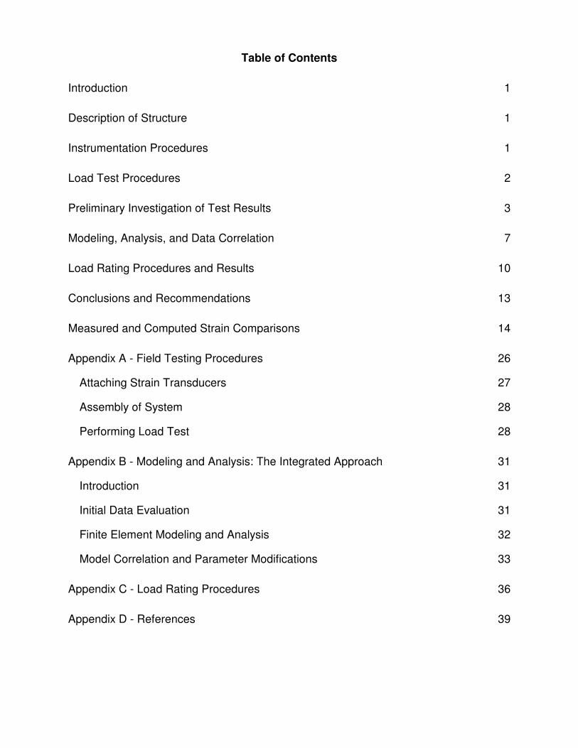
Table of Contents

Introduction 1

Description of Structure 1

Instrumentation Procedures 1

Load Test Procedures 2

Preliminary Investigation of Test Results 3

Modeling, Analysis, and Data Correlation 7

Load Rating Procedures and Results 10

Conclusions and Recommendations 13

Measured and Computed Strain Comparisons 14

Appendix A - Field Testing Procedures 26

Attaching Strain Transducers 27

Assembly of System 28

Performing Load Test 28

Appendix B - Modeling and Analysis: The Integrated Approach 31

Introduction 31

Initial Data Evaluation 31

Finite Element Modeling and Analysis 32

Model Correlation and Parameter Modifications 33

Appendix C - Load Rating Procedures 36

Appendix D - References 39

List of Figures Figure 1 Bonham 1.603 Instrumentation Plan. ................................................................2 Figure 2 Load Configuration of Test Truck ......................................................................3 Figure 3 Stringer 4 @ West Bay - Abutment beam-end not in contact...........................5 Figure 4 Reproducibility of test procedure and data acquisition. .....................................5 Figure 5 Asymmetric Stresses on North and South Truss...............................................6 Figure 6 Strain Histories from Slow and Fast Truck Crossings. ......................................7 Figure 7 Computer generated display of bridge model....................................................9 Figure 8 Measured and Computed Stresses - North Truss L0-L2.................................14 Figure 9 Measured and Computed Stresses - North Truss L2-L4.................................15 Figure 10 Measured and Computed Stresses - North Truss L4-L4'. .............................15 Figure 11 Measured and Computed Stresses - North Truss L0-U1. .............................16 Figure 12 Measured and Computed Stresses - North Truss U1-U3..............................16 Figure 13 Measured and Computed Stresses - North Truss U3-U5..............................17 Figure 14 Measured and Computed Stresses - North Truss U1-L2. .............................17 Figure 15 Measured and Computed Stresses - North Truss L2-U3. .............................18 Figure 16 Measured and Computed Stresses - South Truss L0-L2. .............................18 Figure 17 Measured and Computed Stresses - South Truss L0-U1..............................19 Figure 18 Measured and Computed Stresses - South Truss U1-U3. ............................19 Figure 19 Measured and Computed Stresses - South Truss U1-L2..............................20 Figure 20 Measured and Computed Stresses - Stringer 2 Midspan Bay 1. ..................20 Figure 21 Measured and Computed Stresses - Stringer 3 Midspan Bay 1. ..................21 Figure 22 Measured and Computed Stresses - Stringer 4 Midspan Bay 1. ..................21 Figure 23 Measured and Computed Stresses - Stringer 5 Midspan Bay 1. ..................22 Figure 24 Measured and Computed Stresses - Stringer 6 Midspan Bay 1. ..................22 Figure 25 Measured and Computed Stresses - Stringer 7 Midspan Bay 1. ..................23 Figure 26 Measured and Computed Stresses - Stringer 8 Midspan Bay 1. ..................23 Figure 27 Measured and Computed Stresses - Stringer 9 Midspan Bay 1. ..................24 Figure 28 Measured and Computed Stresses - Stringer 7 Midspan Bay 2. ..................24 Figure 29 Measured and Computed Stresses - Floor Beam at Midspan.......................25 Figure 30 Measured and Computed Stresses - Floor Beam at Quarter Span...............25 Figure 31 Typical Deck Layout for Load Position Monitoring ........................................29 Figure 32 Illustration of Neutral Axis and Curvature Calculations .................................32 Figure 33 AASHTO rating and posting load configurations. ..........................................38

List of Tables Table 1 Maximum measured stresses on truss, stringers and floor beam. .....................7 Table 2 Initial and Final Values of Variable Parameters..................................................9 Table 3 Accuracy of initial and refined models ................................................................9 Table 4 Inventory and Operating Component Capacities..............................................11 Table 5 Inventory and Operating Load Rating Factors for H-20 (20 tons).....................12 Table 6 Inventory and Operating Load Rating Factors for HS-20 (36 tons) ..................12 Table 7 Measured Lateral Distribution Factor for Stringers. ..........................................13 Table 8. Error Functions................................................................................................34

1

Introduction The Bonham 1.603 steel truss bridge was selected for load testing by the Butler County Engineers Office (BCEO) because it was representative of several structures currently posted with restricted load limits. The structure was built in the 1950's and was based on a standard pony truss design with an H-15 load requirement.

Description of Structure Structure Identification Bonham Road 1.603 Location Bonham Rd. Butler County, Ohio Structure Type 5 panel steel pony truss Span Length(s) 69'-0" Skew Perpendicular Roadway/Structure Widths 24'-0" / 25'-6" Truss Connections Welded connections with gusset plates. Stringer Spacing 9 stringers @ 2'-8" Deck type 10 Ga. corrugated steel deck filled with asphalt. Stringers W12x31 typical Exterior Beams Pony truss: 8'-0" deep Abutments Concrete abutment with steel plates providing truss

bearings. No pin or roller mechanisms. Structural Steel Fy = 33 ksi, E=29000 ksi ASTM A-7 Typical. Comments Truss in good to excellent condition. Significant rust and

corrosion on floor deck, stringers, and floor beams.

Instrumentation Procedures The primary goal of the instrumentation plan was to measure the live-load response behavior of the main truss members and to determine the load distribution characteristics of the floor system. The superstructure of the bridge was instrumented with 32 re-usable strain transducers as shown in Figure 1. Based on previous tests on similar trusses, it was known that the truss connections would resist moment and must be analyzed as semi-rigid frames as opposed to being pinned (free rotation). In general, truss member gages were located as near to the cross-sectional centroid to determine the axial force experienced by each member and minimize the effects of bending. Floor beam and stringer gages were typically attached to the bottom flange to measure the strain at the extreme tension fiber. Additional gages were attached to the top flange at several stringer cross-sections to verify that the beams were non-composite with the deck and to detect any unusual responses. Based on the construction details of the superstructure and prior experience with similar structures, it was desired to obtain the following stiffness parameters: • Determine the axial resistance of truss support conditions. • Floor system contribution to the bottom chord stiffness. • Transverse load distribution provided by the corrugated steel deck.

2

Evaluation of these parameters was necessary to accurately assess the load effect on each component due to an applied load condition.

Figure 1 Bonham 1.603 Instrumentation Plan.

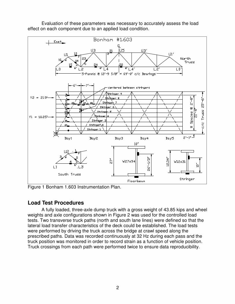
Load Test Procedures A fully loaded, three-axle dump truck with a gross weight of 43.85 kips and wheel weights and axle configurations shown in Figure 2 was used for the controlled load tests. Two transverse truck paths (north and south lane lines) were defined so that the lateral load transfer characteristics of the deck could be established. The load tests were performed by driving the truck across the bridge at crawl speed along the prescribed paths. Data was recorded continuously at 32 Hz during each pass and the truck position was monitored in order to record strain as a function of vehicle position. Truck crossings from each path were performed twice to ensure data reproducibility.

3

11.0 Kips 27.90 Kips

6.5’ 6.1’

12.0’ 4.3’

Axle loads:

Figure 2 Load Configuration of Test Truck All of the instrumentation and testing procedures were completed on August 13th, 1998 with traffic control and a loading vehicle being supplied by BCEO.

Preliminary Investigation of Test Results A visual examination of the field data was first performed to assess the quality of the data and to make a qualitative assessment of the bridge’s live-load response. Conclusions made directly from the field data were: • All responses were primarily elastic. Readings from all top chord, diagonal, floor-

beam and stringer gages returned to zero after each load cycle. Slight residual tension was present in some of the bottom chord gages indicating friction in the truss bearing pads. The residual strains were in the range of 2% of the maximum bottom chord strain.

• Midspan strain histories obtained from interior Stringers 4, 5, and 6 indicated that the stringer ends are not firmly seated at the West abutment bearing locations. Strains obtained from the midspan, bottom-flange gage locations in Bay 1 initially went into compression (negative moment) when the axles where on the west-end of the stringers. This response could only be caused by the beam not being in contact with the abutment beam seat. The beam to be pushed down to make contact with the bearing. Once contact was made with the abutment, the interior stringer responses were similar to the other stringers. The reversal of flexural responses on Stringer 4 can be seen in Figure 3.

• Reproducibility of the load responses from identical truck crossings was excellent as shown in Figure 4. Some differences in load response were detected at the bottom chord near the abutment. These gages also showed the largest degree of inelastic behavior. These responses indicate that some movement does occur in the truss bearings, the slight nonlinear and inelastic behavior is due to the friction in the support system.

• The end bottom chord member (L0-L2) went into compression while the truck was on the first span indicating that the truss support conditions have a significant amount of axial force resistance. This response implies that pin/roller support conditions cannot be assumed in a subsequent analyses.

4

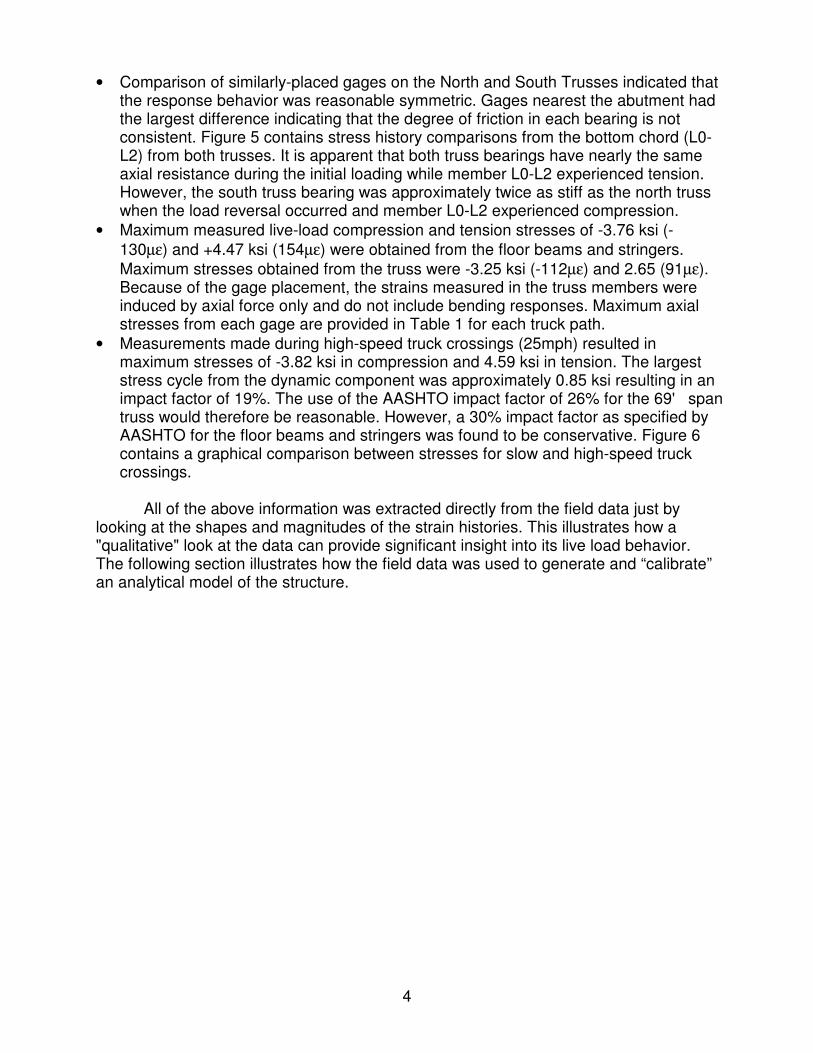
• Comparison of similarly-placed gages on the North and South Trusses indicated that the response behavior was reasonable symmetric. Gages nearest the abutment had the largest difference indicating that the degree of friction in each bearing is not consistent. Figure 5 contains stress history comparisons from the bottom chord (L0-L2) from both trusses. It is apparent that both truss bearings have nearly the same axial resistance during the initial loading while member L0-L2 experienced tension. However, the south truss bearing was approximately twice as stiff as the north truss when the load reversal occurred and member L0-L2 experienced compression.

• Maximum measured live-load compression and tension stresses of -3.76 ksi (-130µε) and +4.47 ksi (154µε) were obtained from the floor beams and stringers. Maximum stresses obtained from the truss were -3.25 ksi (-112µε) and 2.65 (91µε). Because of the gage placement, the strains measured in the truss members were induced by axial force only and do not include bending responses. Maximum axial stresses from each gage are provided in Table 1 for each truck path.

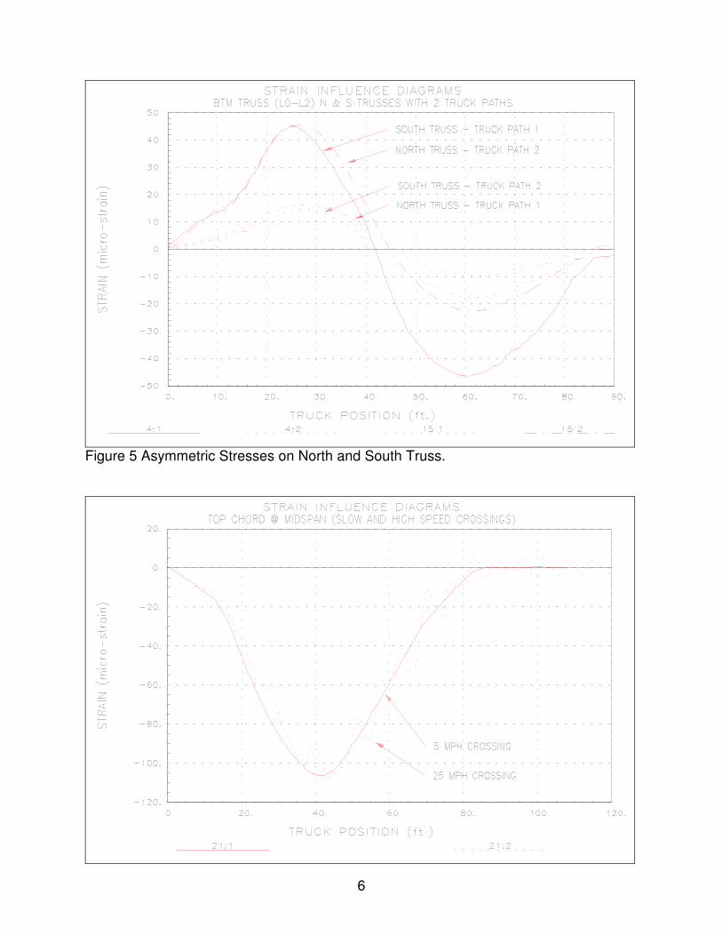
• Measurements made during high-speed truck crossings (25mph) resulted in maximum stresses of -3.82 ksi in compression and 4.59 ksi in tension. The largest stress cycle from the dynamic component was approximately 0.85 ksi resulting in an impact factor of 19%. The use of the AASHTO impact factor of 26% for the 69' span truss would therefore be reasonable. However, a 30% impact factor as specified by AASHTO for the floor beams and stringers was found to be conservative. Figure 6 contains a graphical comparison between stresses for slow and high-speed truck crossings.

All of the above information was extracted directly from the field data just by looking at the shapes and magnitudes of the strain histories. This illustrates how a "qualitative" look at the data can provide significant insight into its live load behavior. The following section illustrates how the field data was used to generate and “calibrate” an analytical model of the structure.

5

Figure 3 Stringer 4 @ West Bay - Abutment beam-end not in contact.

Figure 4 Reproducibility of test procedure and data acquisition.

6

Figure 5 Asymmetric Stresses on North and South Truss.

7

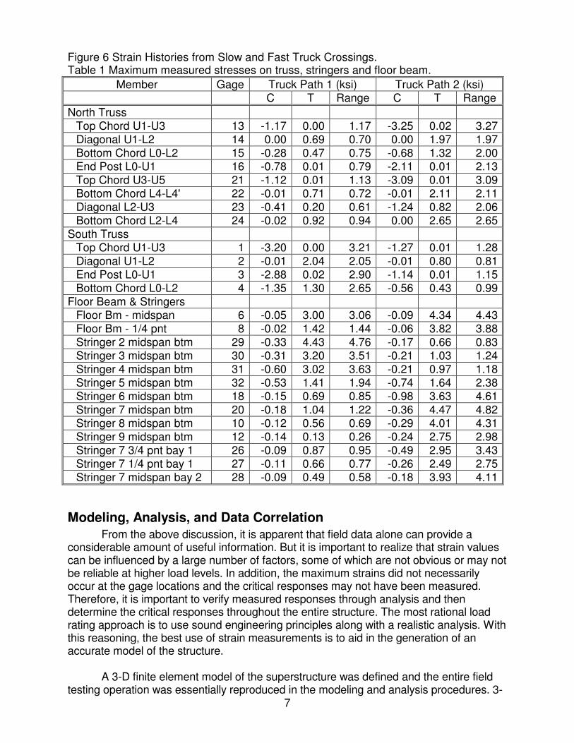
Figure 6 Strain Histories from Slow and Fast Truck Crossings. Table 1 Maximum measured stresses on truss, stringers and floor beam.

Member Gage Truck Path 1 (ksi) Truck Path 2 (ksi) C T Range C T Range North Truss

Top Chord U1-U3 13 -1.17 0.00 1.17 -3.25 0.02 3.27 Diagonal U1-L2 14 0.00 0.69 0.70 0.00 1.97 1.97 Bottom Chord L0-L2 15 -0.28 0.47 0.75 -0.68 1.32 2.00 End Post L0-U1 16 -0.78 0.01 0.79 -2.11 0.01 2.13 Top Chord U3-U5 21 -1.12 0.01 1.13 -3.09 0.01 3.09 Bottom Chord L4-L4' 22 -0.01 0.71 0.72 -0.01 2.11 2.11 Diagonal L2-U3 23 -0.41 0.20 0.61 -1.24 0.82 2.06 Bottom Chord L2-L4 24 -0.02 0.92 0.94 0.00 2.65 2.65

South Truss Top Chord U1-U3 1 -3.20 0.00 3.21 -1.27 0.01 1.28 Diagonal U1-L2 2 -0.01 2.04 2.05 -0.01 0.80 0.81 End Post L0-U1 3 -2.88 0.02 2.90 -1.14 0.01 1.15 Bottom Chord L0-L2 4 -1.35 1.30 2.65 -0.56 0.43 0.99

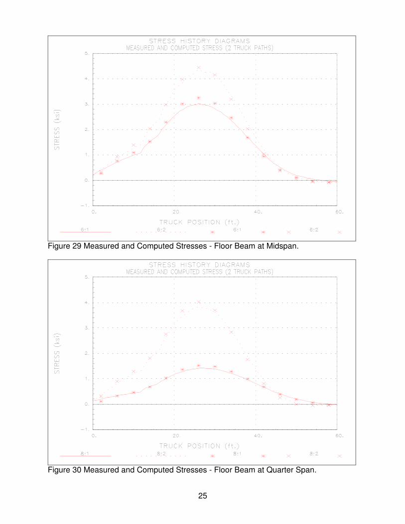
Floor Beam & Stringers Floor Bm - midspan 6 -0.05 3.00 3.06 -0.09 4.34 4.43 Floor Bm - 1/4 pnt 8 -0.02 1.42 1.44 -0.06 3.82 3.88 Stringer 2 midspan btm 29 -0.33 4.43 4.76 -0.17 0.66 0.83 Stringer 3 midspan btm 30 -0.31 3.20 3.51 -0.21 1.03 1.24 Stringer 4 midspan btm 31 -0.60 3.02 3.63 -0.21 0.97 1.18 Stringer 5 midspan btm 32 -0.53 1.41 1.94 -0.74 1.64 2.38 Stringer 6 midspan btm 18 -0.15 0.69 0.85 -0.98 3.63 4.61 Stringer 7 midspan btm 20 -0.18 1.04 1.22 -0.36 4.47 4.82 Stringer 8 midspan btm 10 -0.12 0.56 0.69 -0.29 4.01 4.31 Stringer 9 midspan btm 12 -0.14 0.13 0.26 -0.24 2.75 2.98 Stringer 7 3/4 pnt bay 1 26 -0.09 0.87 0.95 -0.49 2.95 3.43 Stringer 7 1/4 pnt bay 1 27 -0.11 0.66 0.77 -0.26 2.49 2.75 Stringer 7 midspan bay 2 28 -0.09 0.49 0.58 -0.18 3.93 4.11

Modeling, Analysis, and Data Correlation From the above discussion, it is apparent that field data alone can provide a considerable amount of useful information. But it is important to realize that strain values can be influenced by a large number of factors, some of which are not obvious or may not be reliable at higher load levels. In addition, the maximum strains did not necessarily occur at the gage locations and the critical responses may not have been measured. Therefore, it is important to verify measured responses through analysis and then determine the critical responses throughout the entire structure. The most rational load rating approach is to use sound engineering principles along with a realistic analysis. With this reasoning, the best use of strain measurements is to aid in the generation of an accurate model of the structure. A 3-D finite element model of the superstructure was defined and the entire field testing operation was essentially reproduced in the modeling and analysis procedures. 3-

8

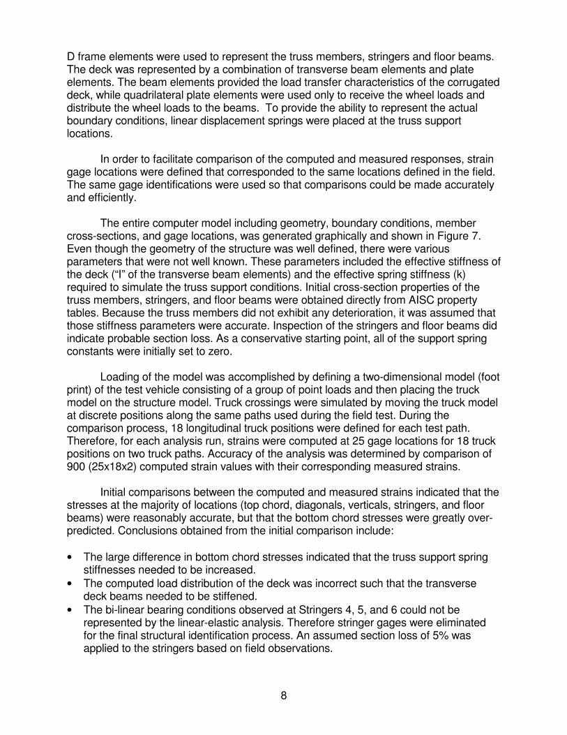
D frame elements were used to represent the truss members, stringers and floor beams. The deck was represented by a combination of transverse beam elements and plate elements. The beam elements provided the load transfer characteristics of the corrugated deck, while quadrilateral plate elements were used only to receive the wheel loads and distribute the wheel loads to the beams. To provide the ability to represent the actual boundary conditions, linear displacement springs were placed at the truss support locations. In order to facilitate comparison of the computed and measured responses, strain gage locations were defined that corresponded to the same locations defined in the field. The same gage identifications were used so that comparisons could be made accurately and efficiently. The entire computer model including geometry, boundary conditions, member cross-sections, and gage locations, was generated graphically and shown in Figure 7. Even though the geometry of the structure was well defined, there were various parameters that were not well known. These parameters included the effective stiffness of the deck (“I” of the transverse beam elements) and the effective spring stiffness (k) required to simulate the truss support conditions. Initial cross-section properties of the truss members, stringers, and floor beams were obtained directly from AISC property tables. Because the truss members did not exhibit any deterioration, it was assumed that those stiffness parameters were accurate. Inspection of the stringers and floor beams did indicate probable section loss. As a conservative starting point, all of the support spring constants were initially set to zero. Loading of the model was accomplished by defining a two-dimensional model (foot print) of the test vehicle consisting of a group of point loads and then placing the truck model on the structure model. Truck crossings were simulated by moving the truck model at discrete positions along the same paths used during the field test. During the comparison process, 18 longitudinal truck positions were defined for each test path. Therefore, for each analysis run, strains were computed at 25 gage locations for 18 truck positions on two truck paths. Accuracy of the analysis was determined by comparison of 900 (25x18x2) computed strain values with their corresponding measured strains. Initial comparisons between the computed and measured strains indicated that the stresses at the majority of locations (top chord, diagonals, verticals, stringers, and floor beams) were reasonably accurate, but that the bottom chord stresses were greatly over-predicted. Conclusions obtained from the initial comparison include: • The large difference in bottom chord stresses indicated that the truss support spring

stiffnesses needed to be increased. • The computed load distribution of the deck was incorrect such that the transverse

deck beams needed to be stiffened. • The bi-linear bearing conditions observed at Stringers 4, 5, and 6 could not be

represented by the linear-elastic analysis. Therefore stringer gages were eliminated for the final structural identification process. An assumed section loss of 5% was applied to the stringers based on field observations.

9

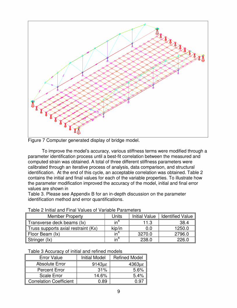
Figure 7 Computer generated display of bridge model. To improve the model’s accuracy, various stiffness terms were modified through a parameter identification process until a best-fit correlation between the measured and computed strain was obtained. A total of three different stiffness parameters were calibrated through an iterative process of analysis, data comparison, and structural identification. At the end of this cycle, an acceptable correlation was obtained. Table 2 contains the initial and final values for each of the variable properties. To illustrate how the parameter modification improved the accuracy of the model, initial and final error values are shown in Table 3. Please see Appendix B for an in-depth discussion on the parameter identification method and error quantifications. Table 2 Initial and Final Values of Variable Parameters

Member Property Units Initial Value Identified Value Transverse deck beams (Ix) in4 11.3 38.4 Truss supports axial restraint (Kx) kip/in 0.0 1250.0 Floor Beam (Ix) in4 3270.0 2796.0 Stringer (Ix) in4 238.0 226.0 Table 3 Accuracy of initial and refined models

Error Value Initial Model Refined Model Absolute Error 9143µε 4363µε Percent Error 31% 5.6% Scale Error 14.6% 5.4%

Correlation Coefficient 0.89 0.97

10

At this point, the model has been “calibrated” to the field measurements. Since the load responses of the model are very similar to those of the actual structure, it can be assumed that the stiffness and load transfer characteristics are correct. This method of “integrating” the analysis with experimental results now provides a quantitative and rational basis for further evaluation. Discussion of Results The accuracy obtained by this evaluation process was typical of steel truss structures. The most important observations made from the load test data evaluation and during the parameter identification process are as follows: • The truss support pads do not allow free longitudinal translation during normal traffic

loading. The overall effect of this condition is that the bottom chord tension stresses are greatly reduced because much of the axial force is transmitted into the truss reactions. For example, the midspan bottom chord member (L4-L4') tension forces are reduced by 50% when the bridge is loaded with two HS-20 (model) trucks. The diagonal members are minimally affected, and there is essentially no affect on the top chord and vertical members.

• The welded gusset plate connections cause the trusses to act as a rigid frame rather than a truss with pinned connections. This causes the trusses to be stiffer than would be predicted by a simple truss analysis. It is important to note, however, that the load capacity may not be increased substantially because bending effects must be considered when calculating stresses. The inclusion of bending stresses typically offset the reduction of axial force stresses. While stresses at extreme fibers are not significantly reduced, the stiffness of the truss is increased by the rigid connections and the deflection is reduced compared to a truss with pinned connections.

• The bi-linear support conditions observed from Stringer 4, 5, and 6 at the west-end bay could not be realistically represented by a linear analysis. The support conditions induced unusual responses for the stringers and also had an effect on the lateral distribution of the floor system in the first bay. Typical support conditions will be assumed for subsequent evaluations.

Load Rating Procedures and Results The main reason for producing a field-calibrated model was to have the ability to compute realistic load ratings. Load test results are generally limited to the specific load application. However, given a realistic model, analyses and load ratings can be performed for any load configuration. In this section, a discussion of the load rating procedures is given and load limits are provided for H-20 and HS-20 load configurations. Inventory and operating rating factors were computed using Allowable Stress Design (ASD) procedures. Member capacities were computed for the truss and floor system member using the appropriate AASHTO design specifications. Allowable stresses were computed for A-36 and A-242 steel with appropriate reductions in compression stresses based on the members' KL/r ratios. Member capacities were computed for individual responses such as tension, compression, and bending about each axis and are listed in Table 4.

11

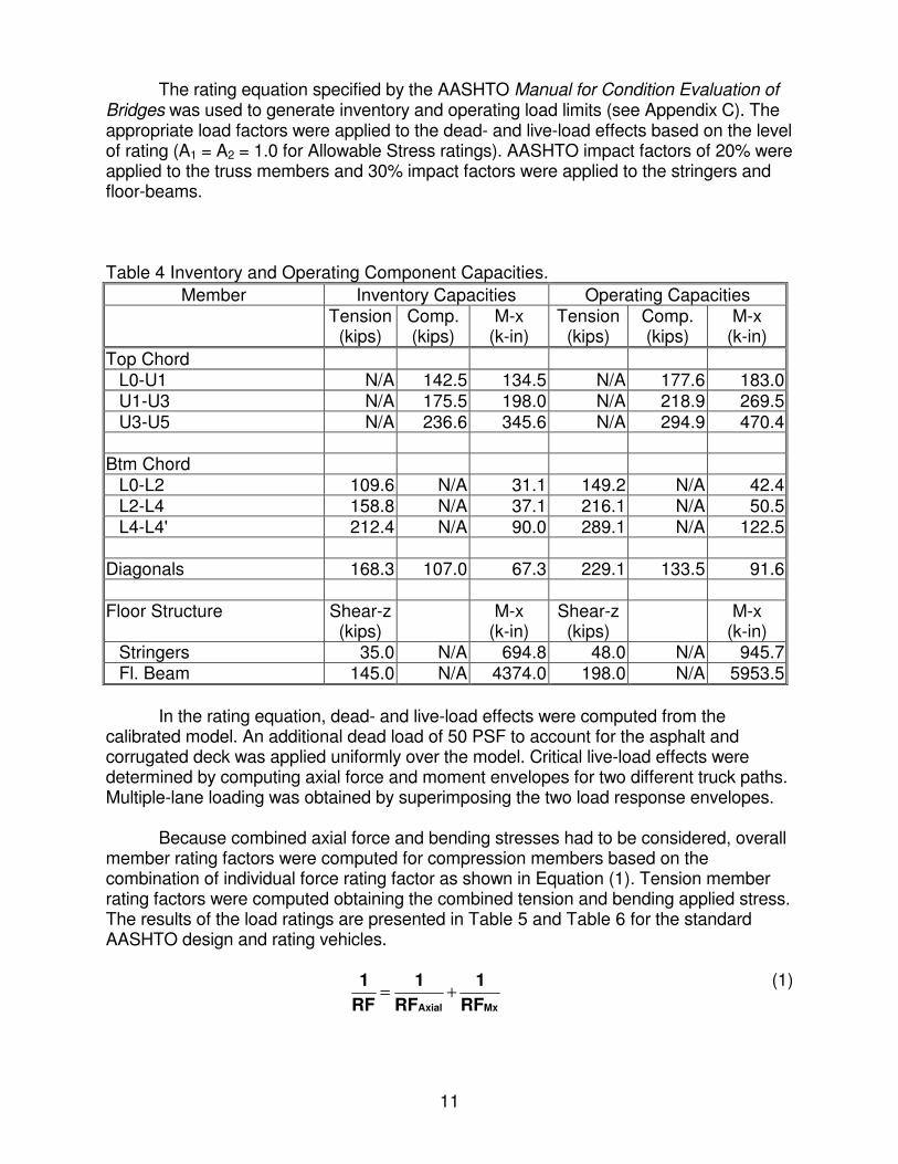
The rating equation specified by the AASHTO Manual for Condition Evaluation of Bridges was used to generate inventory and operating load limits (see Appendix C). The appropriate load factors were applied to the dead- and live-load effects based on the level of rating (A1 = A2 = 1.0 for Allowable Stress ratings). AASHTO impact factors of 20% were applied to the truss members and 30% impact factors were applied to the stringers and floor-beams. Table 4 Inventory and Operating Component Capacities.

Member Inventory Capacities Operating Capacities Tension

(kips) Comp. (kips)

M-x (k-in)

Tension (kips)

Comp. (kips)

M-x (k-in)

Top Chord L0-U1 N/A 142.5 134.5 N/A 177.6 183.0 U1-U3 N/A 175.5 198.0 N/A 218.9 269.5 U3-U5 N/A 236.6 345.6 N/A 294.9 470.4

Btm Chord L0-L2 109.6 N/A 31.1 149.2 N/A 42.4 L2-L4 158.8 N/A 37.1 216.1 N/A 50.5 L4-L4' 212.4 N/A 90.0 289.1 N/A 122.5

Diagonals 168.3 107.0 67.3 229.1 133.5 91.6

Floor Structure Shear-z (kips)

M-x (k-in)

Shear-z (kips)

M-x (k-in)

Stringers 35.0 N/A 694.8 48.0 N/A 945.7 Fl. Beam 145.0 N/A 4374.0 198.0 N/A 5953.5

In the rating equation, dead- and live-load effects were computed from the calibrated model. An additional dead load of 50 PSF to account for the asphalt and corrugated deck was applied uniformly over the model. Critical live-load effects were determined by computing axial force and moment envelopes for two different truck paths. Multiple-lane loading was obtained by superimposing the two load response envelopes. Because combined axial force and bending stresses had to be considered, overall member rating factors were computed for compression members based on the combination of individual force rating factor as shown in Equation (1). Tension member rating factors were computed obtaining the combined tension and bending applied stress. The results of the load ratings are presented in Table 5 and Table 6 for the standard AASHTO design and rating vehicles.

MxAxial RF1

RF1

RF1 +=

(1)

12

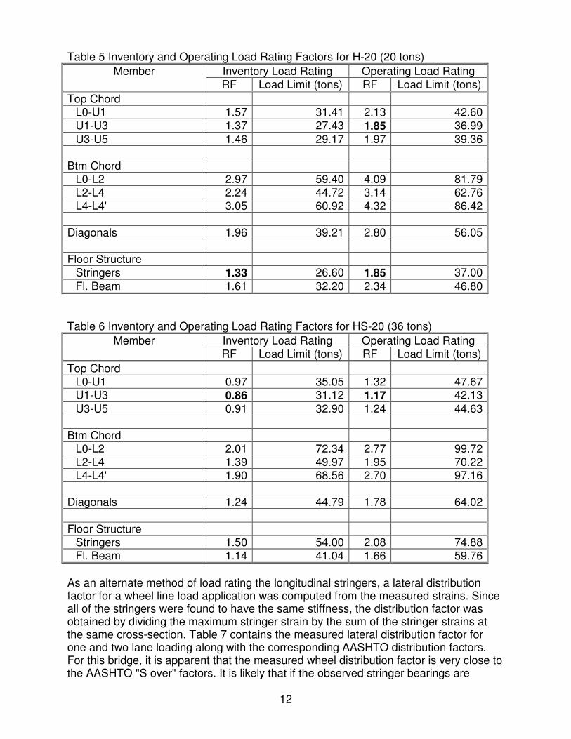
Table 5 Inventory and Operating Load Rating Factors for H-20 (20 tons) Member Inventory Load Rating Operating Load Rating

RF Load Limit (tons) RF Load Limit (tons) Top Chord

L0-U1 1.57 31.41 2.13 42.60 U1-U3 1.37 27.43 1.85 36.99 U3-U5 1.46 29.17 1.97 39.36

Btm Chord L0-L2 2.97 59.40 4.09 81.79 L2-L4 2.24 44.72 3.14 62.76 L4-L4' 3.05 60.92 4.32 86.42

Diagonals 1.96 39.21 2.80 56.05

Floor Structure Stringers 1.33 26.60 1.85 37.00 Fl. Beam 1.61 32.20 2.34 46.80

Table 6 Inventory and Operating Load Rating Factors for HS-20 (36 tons)

Member Inventory Load Rating Operating Load Rating RF Load Limit (tons) RF Load Limit (tons)

Top Chord L0-U1 0.97 35.05 1.32 47.67 U1-U3 0.86 31.12 1.17 42.13 U3-U5 0.91 32.90 1.24 44.63

Btm Chord L0-L2 2.01 72.34 2.77 99.72 L2-L4 1.39 49.97 1.95 70.22 L4-L4' 1.90 68.56 2.70 97.16

Diagonals 1.24 44.79 1.78 64.02

Floor Structure Stringers 1.50 54.00 2.08 74.88 Fl. Beam 1.14 41.04 1.66 59.76

As an alternate method of load rating the longitudinal stringers, a lateral distribution factor for a wheel line load application was computed from the measured strains. Since all of the stringers were found to have the same stiffness, the distribution factor was obtained by dividing the maximum stringer strain by the sum of the stringer strains at the same cross-section. Table 7 contains the measured lateral distribution factor for one and two lane loading along with the corresponding AASHTO distribution factors. For this bridge, it is apparent that the measured wheel distribution factor is very close to the AASHTO "S over" factors. It is likely that if the observed stringer bearings are

13

repaired so that all stringers are in contact with their supports, the lateral distribution will improve slightly. Table 7 Measured Lateral Distribution Factor for Stringers. Distribution Factor Single Lane Load Two Lane Load Measured 0.50 0.61 AASHTO 3.23.2.2 S/5.5 = 0.48 S/4.5 = 0.59

Conclusions and Recommendations From the load rating results, it is apparent that the stringers control the load limits for H-20 loading and the top chord members are critical for HS-20 loading. Tension along the bottom chord is not a critical factor because the tension forces are significantly reduced by the truss reactions. In fact, the end bottom-chord members (L0-L2) are limited by compression even through they are designed to be tension members. Because of the truss construction details, the relatively low tension stresses, and the low traffic volume on this structure, fatigue was not considered to be an important factor and was therefore not included in the load rating calculations. Fatigue may need to be considered on similar bridges that have a more typical truss support system (free to expand), and that have a greater volume of truck traffic. The observed bi-linear support conditions could not be realistically represented with a linear-elastic analysis. Load ratings on the stringers were based on normal bearing conditions. The observed stringer-bearing condition should be confirmed by a visual inspection and repaired if it is found that a gap does exist between the stringers and the beam seats. The effect of the poor beam-seats may be that the stringers resting on their supports carry a higher load percentage than those that are not in contact. Also, large impact forces may be induced when the stringer ends are pushed (or slammed) down onto their bearings, which may have detrimental effects on the abutment integrity. The primary factors determined from the load testing operation, that could not have been determined by a conventional inspection and load rating, were the effects of the truss supports and the frame-like behavior of the trusses. While the support conditions are not typical of most trusses, it does not appear that the axial restraint has any adverse effects on the structure's response behavior. The support conditions provided some benefit in that the bottom chord tension stresses were greatly reduced. However, the overall load ratings were not substantially affected because the top chord members were essentially uninfluenced by the truss boundary conditions. Rating values and information presented in this report are based on the condition of the superstructure at the time of the actual field-testing. No effort has been made to evaluate the condition of the substructure components and no implication has been made concerning substructure load capacity.

14

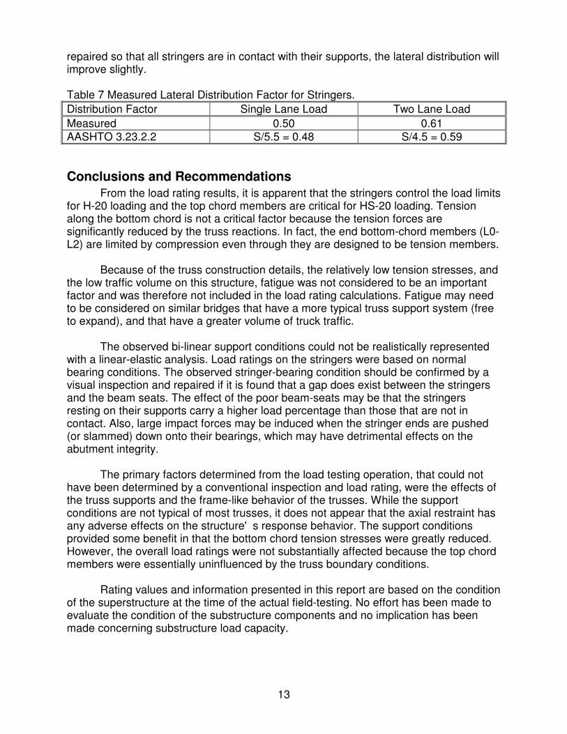
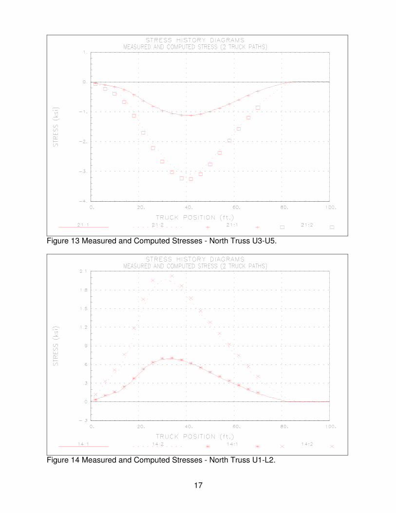
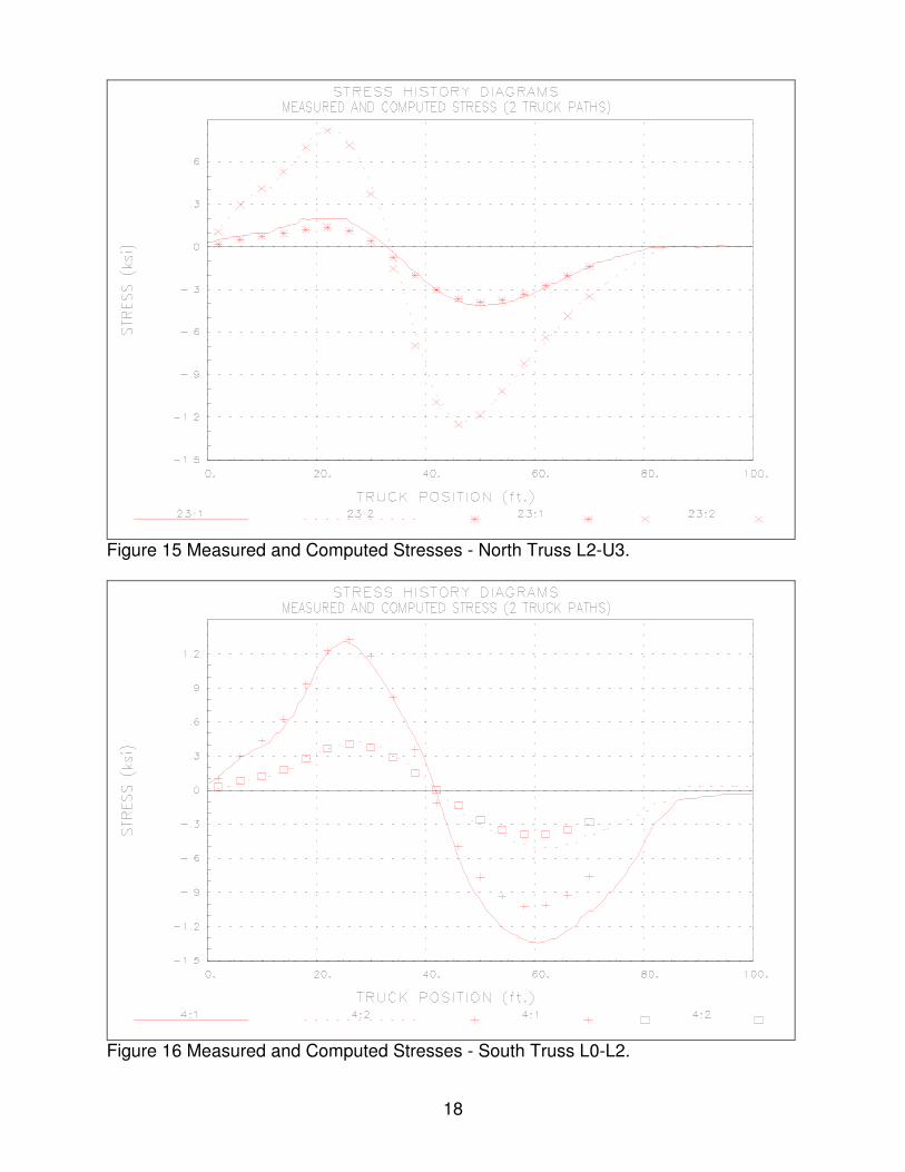
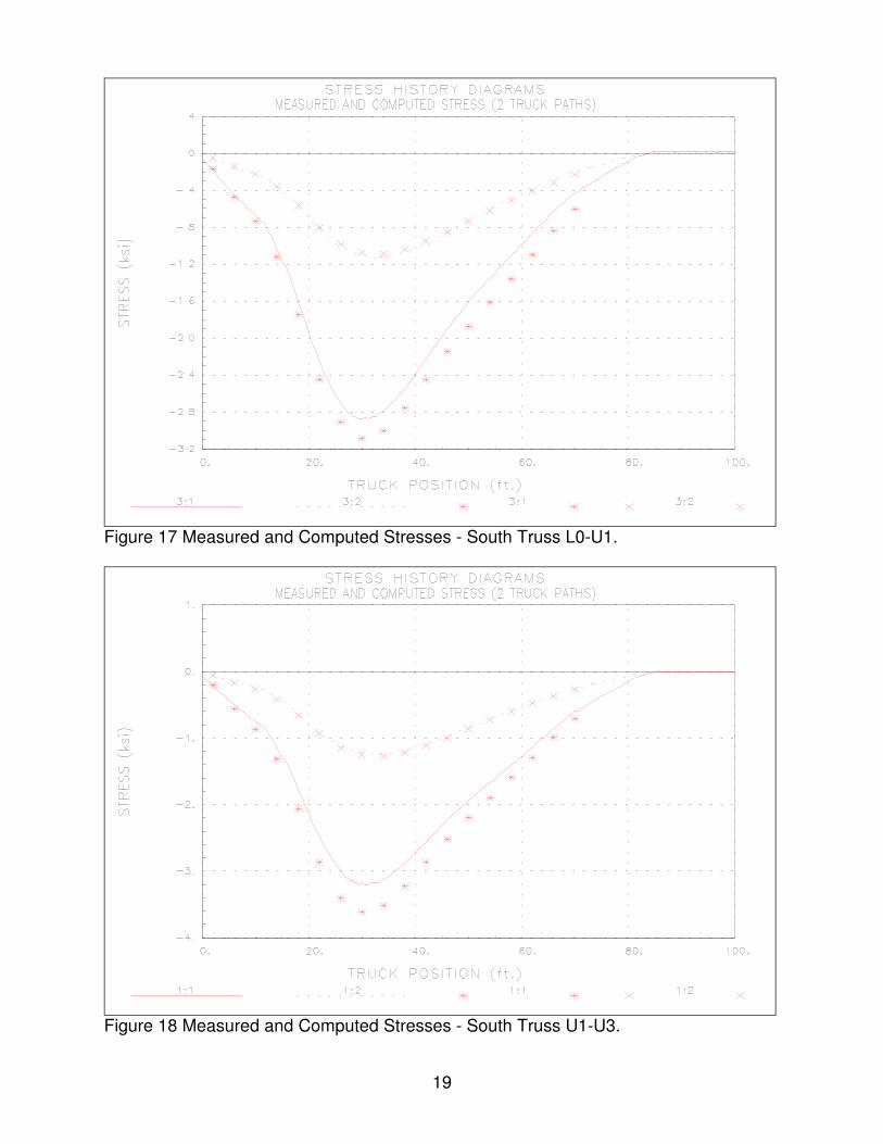
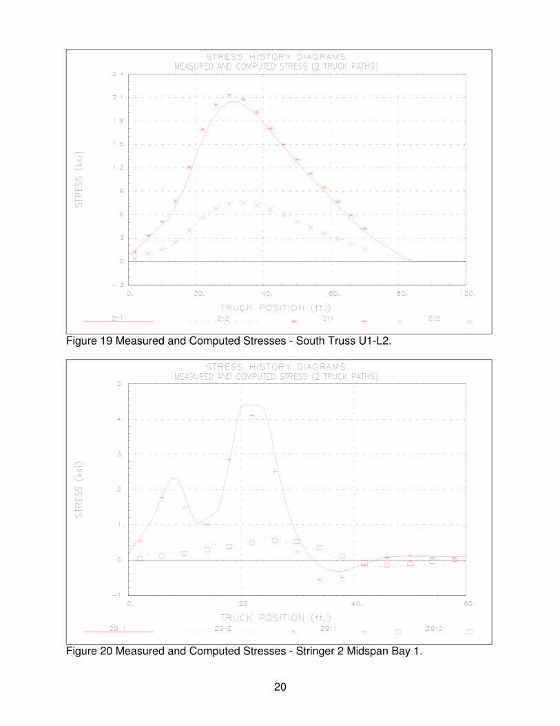
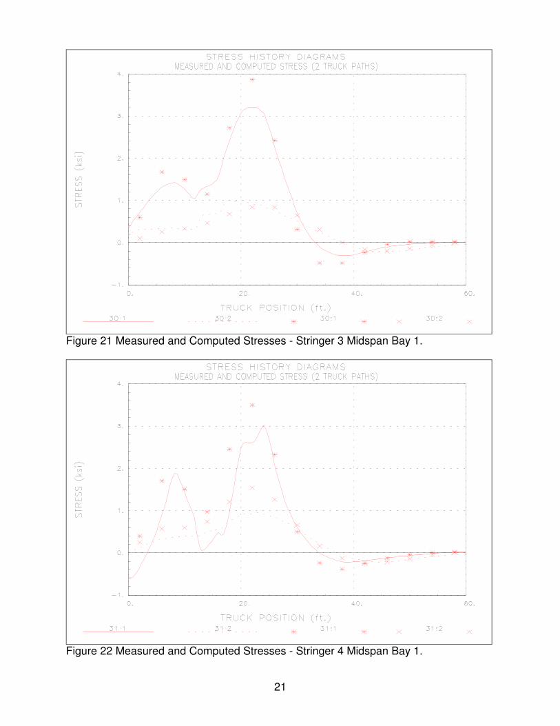
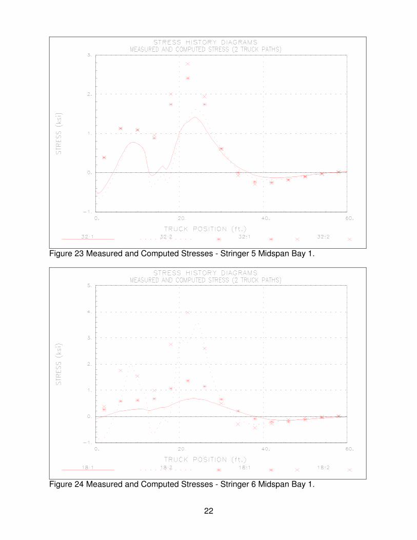
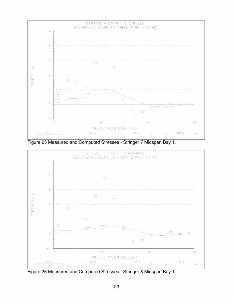
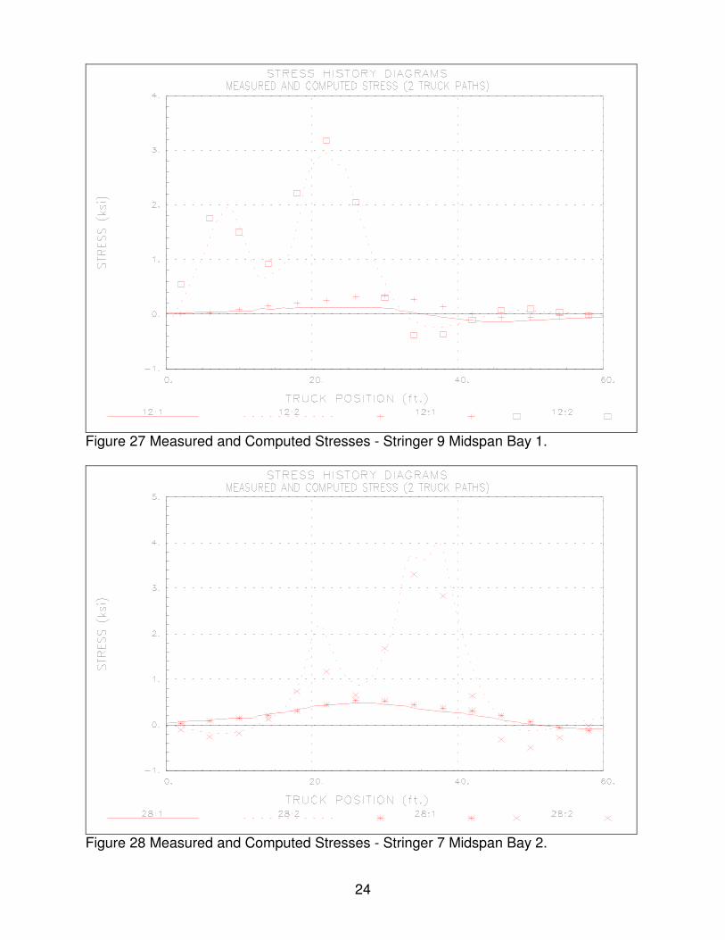
Measured and Computed Strain Comparisons While statistical terms provide a means of evaluating the relative accuracy of various modeling procedures or help determine the improvement of a model during a calibration process, the best conceptual measure of a model's accuracy is by visual examination of the response histories. The following graphs contain measured and computed stress histories from each truck path. In each graph the continuous lines represent the measured stress as a function of truck position as it traveled across the bridge. Computed stresses are shown as markers at discrete truck intervals. The two sets of data for each gage represent the two different truck paths.

Figure 8 Measured and Computed Stresses - North Truss L0-L2.

15

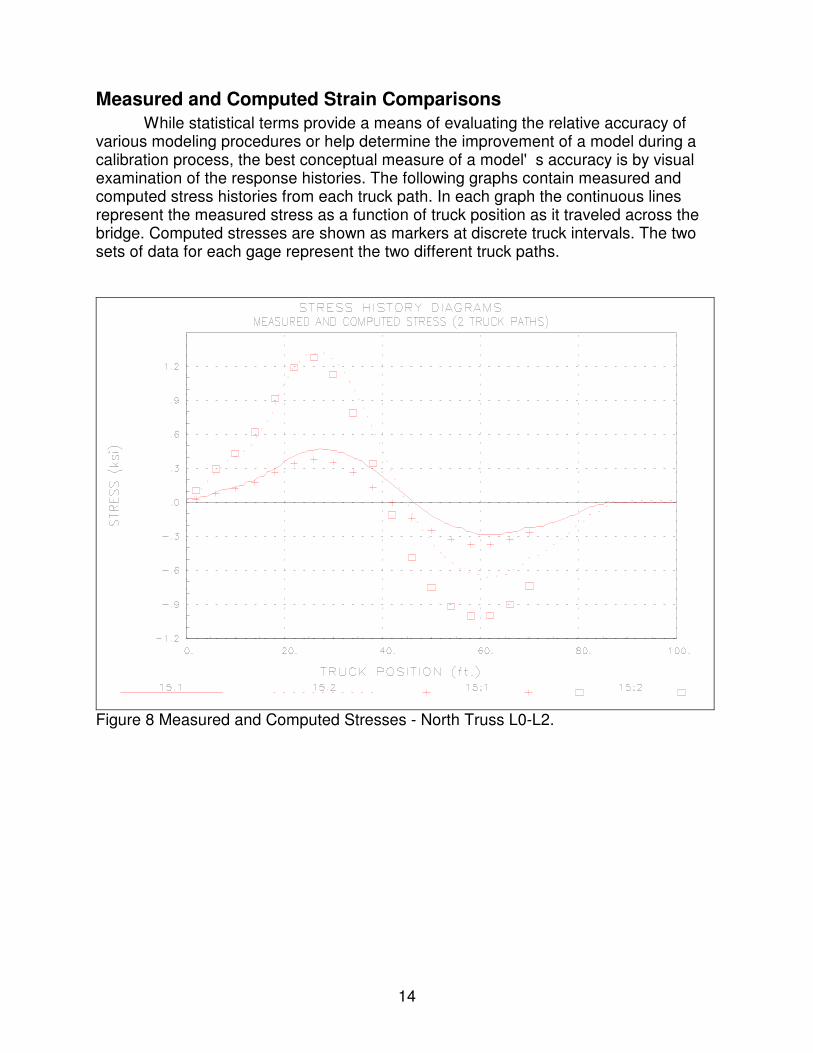
Figure 9 Measured and Computed Stresses - North Truss L2-L4.

Figure 10 Measured and Computed Stresses - North Truss L4-L4'.

16

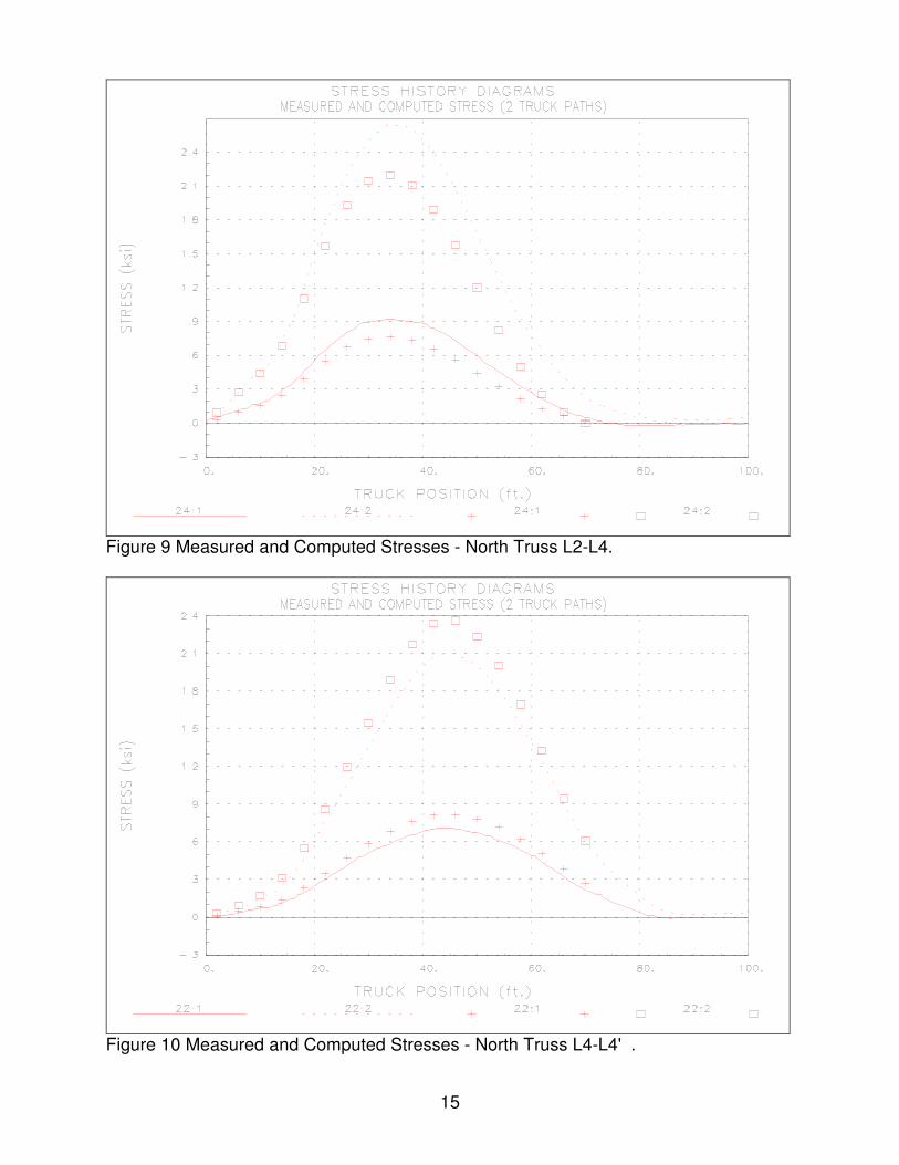
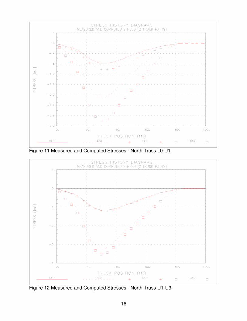
Figure 11 Measured and Computed Stresses - North Truss L0-U1.

Figure 12 Measured and Computed Stresses - North Truss U1-U3.

17

Figure 13 Measured and Computed Stresses - North Truss U3-U5.

Figure 14 Measured and Computed Stresses - North Truss U1-L2.

18

Figure 15 Measured and Computed Stresses - North Truss L2-U3.

Figure 16 Measured and Computed Stresses - South Truss L0-L2.

19

Figure 17 Measured and Computed Stresses - South Truss L0-U1.

Figure 18 Measured and Computed Stresses - South Truss U1-U3.

20

Figure 19 Measured and Computed Stresses - South Truss U1-L2.

Figure 20 Measured and Computed Stresses - Stringer 2 Midspan Bay 1.

21

Figure 21 Measured and Computed Stresses - Stringer 3 Midspan Bay 1.

Figure 22 Measured and Computed Stresses - Stringer 4 Midspan Bay 1.

22

Figure 23 Measured and Computed Stresses - Stringer 5 Midspan Bay 1.

Figure 24 Measured and Computed Stresses - Stringer 6 Midspan Bay 1.

23

Figure 25 Measured and Computed Stresses - Stringer 7 Midspan Bay 1.

Figure 26 Measured and Computed Stresses - Stringer 8 Midspan Bay 1.

24

Figure 27 Measured and Computed Stresses - Stringer 9 Midspan Bay 1.

Figure 28 Measured and Computed Stresses - Stringer 7 Midspan Bay 2.

25

Figure 29 Measured and Computed Stresses - Floor Beam at Midspan.

Figure 30 Measured and Computed Stresses - Floor Beam at Quarter Span.

26

Appendix A - Field Testing Procedures The motivation for developing a relatively easy-to-implement field testing system was to allow short and medium span bridges to be tested on a routine basis. Original development of the hardware was started in 1988 at the University of Colorado under a contract with the Pennsylvania Department of Transportation (PennDOT). Subsequent to that project, the Integrated technique was refined on another study funded by the Federal Highway Administration (FHWA) in which 35 bridges located on the Interstate system throughout the country were tested and evaluated. Further refinement has been implemented over the last several years through testing and evaluating several more bridges, lock gates, and other structures. The real key to being able to complete the field testing quickly is the use of strain transducers (rather than standard foil strain gages) that can be attached to the structural members in just a few minutes. These sensors were originally developed for monitoring dynamic strains on foundation piles during the driving process. They have been adapted for use in structural testing through special modifications, and have a 3 to 4 percent accuracy, and are periodically re-calibrated to NIST standards. In addition to the strain sensors, the data acquisition hardware has been designed specifically for field use through the use of rugged cables and military-style connectors. This allows quick assembly of the system and keeps bookkeeping to a minimum. The analog-to-digital converter (A/D) is an off-the-shelf-unit, but all signal conditioning, amplification, and balancing hardware has been specially designed for structural testing. The test software has been written to allow easy configuration (test length, etc.) and operation. The end result is a system that can be used by people other than computer experts or electrical engineers. Other enhancements include the use of a remote-control position indicator. As the test vehicle crosses the structure, one of the testing personnel walks along-side and depresses a button on the communication radio each time the front axle of the vehicle crosses one of the chalk lines laid out on the deck. This action sends a signal to the strain measurement system which receives it and puts a mark in the data. This allows the field strains to be compared to analytical strains as a function of vehicle position, not only as a function of time. The use of a moving load as opposed to placing the truck at discrete locations has two major benefits. First, the testing can be completed much quicker, meaning there is less impact on traffic. Second, and more importantly, much more information can be obtained (both quantitative and qualitative). Discontinuities or unusual responses in the strain histories, which are often signs of distress, can be easily detected. Since the load position is monitored as well, it is easy to determine what loading conditions cause the observed effects. If readings are recorded only at discreet truck locations, the risk of losing information between the points is great. The advantages of continuous readings have been proven over and over again. The following list of procedures have been reproduced from the BDI Structural Testing System (STS) Operation Manual. This outline is intended to describe the general procedures used for completing a successful field test on a highway bridge using the BDI-STS. Other types of structures can be tested as well with only slight deviations from the directions given here.

27

Once a tentative instrumentation plan has been developed for the structure in question, the strain transducers must be attached and the STS prepared for running the test.

Attaching Strain Transducers There are two methods for attaching the strain transducers to the structural members: C-clamping or with tabs and adhesive. For steel structures, quite often the transducers can be clamped directly to the steel flanges of rolled sections or plate girders. If significant lateral bending is assumed to be present, then one transducer may be clamped to each edge of the flange. If the transducer is to be clamped, insure that the clamp is centered over the mounting holes. In general, the transducers can be clamped directly to painted surfaces. However, if the surface being clamped to is rough or has very thick paint, it should be cleaned first with a grinder. The alternative to clamping is the tab attachment method outlined below. 1. Place two tabs in mounting jig. Place transducer over mounts and tighten the 1/4-20

nuts until they are snug (approximately 50 in-lb.). This procedure allows the tabs to mounted without putting stress on the transducer itself. When attaching transducers to R/C members, transducer extensions are used to obtain a longer gage length. In this case the extension is bolted to one end of the transducer and the tabs are bolted to the free ends of the transducer and the extension.

2. Mark the centerline of the transducer location on the structure. Place marks 1-1/2

inches on either side of the centerline and using a hand grinder, remove paint or scale from these areas. If attaching to concrete, lightly grind the surface to remove any scale. If the paint is quite thick, use a chisel to remove most of it before grinding.

3. Very lightly grind the bottom of the transducer tabs to remove any oxidation or other

contaminants. 4. Apply a thin line of adhesive to the bottom of each transducer tab. 5. Spray each tab and the contact area on the structural member with the adhesive

accelerator. 6. Mount transducer in its proper location and apply a light force to the tabs (not the

center of the transducer) for approximately 10 seconds. If the above steps are followed, it should be possible to mount each transducer in approximately five minutes. When the test is complete, carefully loosen the 1/4-20 nuts from the tabs and remove transducer. If one is not careful, the tab will pop loose from the structure and the transducer may be damaged. Use vice grips to remove the tabs from the structure.

28

allow four transducers to be plugged in. Each STS unit can be easily clamped to the bridge girders. If the structure is concrete and no flanges are available to set the STS units on, transducer tabs glued to the structure and plastic zip-ties or small wire can be used to hold them up. Since the transducers will identify themselves to the system, there is no special order that they must follow. The only information that must be recorded is the transducer serial number and its location on the structure. Large cables are provided which can be connected between the STS units. The maximum length between STS units is 50ft (15m). If several gages are in close proximity to each other, then the STS units can be plugged directly to each other without the use of a cable. All connectors will "click" when the connection has been completed properly. Once all of the STS units have been connected in series, one cable must be run and connected to the power supply located near the PC. Connect the 9-pin serial cable between the computer and the power supply. The position indicator is then assembled and the system connected to a power source (either 12VDC or 120-240AC). The system is now ready to acquire data.

Performing Load Test The general testing sequence is as follows: 1. Transducers are mounted and the system is connected together and turned on. 2. The deck is marked out for each truck pass. Locate the point on the deck directly

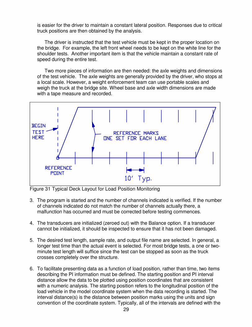
above the first bearing for one of the fascia beams. If the bridge is skewed, the first point encountered from the direction of travel is used and an imaginary line extended across and normal to the roadway as shown in Figure 31. All tests are started from this line. In order to track the position of the loading vehicle on the bridge during the test, an X-Y coordinate system, with the origin at the selected reference point is laid out. Longitudinal marks are placed with chalk powder the length of the bridge in even increments. For spans less than 100-ft (30.5-m), 10-ft (3.05-m) increments are used, although for very short spans, use 5-ft (1.5-m) For longer spans, marks are placed at 20-foot (6.1-m) intervals. This is done for each lane that the truck travels over. A typical deck layout is shown in Figure 31.

In addition to monitoring the longitudinal position, the vehicle's transverse position must be known. The transverse truck position is kept uniform by first aligning the truck in the center of the lane where it would normally travel at highway speed. Next, a chalk mark is made on the deck locating the transverse location of the driver's side front wheel. By making a measurement from this mark to the reference point, the transverse ("Y") position of the truck is always known. The truck is aligned on this mark for all subsequent tests in this lane. For two lane bridges with shoulders, tests are run on the shoulder (driver's side front wheel along the white line) and in the center of each lane. If the bridge has only two lanes and very little shoulder, tests are run in the center of each lane only. If the purpose of the test is to calibrate a computer model, it is sometimes more convenient to simply use the lane lines as guides since it

Assembly of System Once the transducers have been mounted, they should be connected into an STS unit. The STS units should be placed near the transducer locations in such a manner to

29

is easier for the driver to maintain a constant lateral position. Responses due to critical truck positions are then obtained by the analysis.

The driver is instructed that the test vehicle must be kept in the proper location on the bridge. For example, the left front wheel needs to be kept on the white line for the shoulder tests. Another important item is that the vehicle maintain a constant rate of speed during the entire test.

Two more pieces of information are then needed: the axle weights and dimensions of the test vehicle. The axle weights are generally provided by the driver, who stops at a local scale. However, a weight enforcement team can use portable scales and weigh the truck at the bridge site. Wheel base and axle width dimensions are made with a tape measure and recorded.

Figure 31 Typical Deck Layout for Load Position Monitoring 3. The program is started and the number of channels indicated is verified. If the number

of channels indicated do not match the number of channels actually there, a malfunction has occurred and must be corrected before testing commences.

4. The transducers are initialized (zeroed out) with the Balance option. If a transducer

cannot be initialized, it should be inspected to ensure that it has not been damaged. 5. The desired test length, sample rate, and output file name are selected. In general, a

longer test time than the actual event is selected. For most bridge tests, a one or two-minute test length will suffice since the test can be stopped as soon as the truck crosses completely over the structure.

6. To facilitate presenting data as a function of load position, rather than time, two items

describing the PI information must be defined. The starting position and PI interval distance allow the data to be plotted using position coordinates that are consistent with a numeric analysis. The starting position refers to the longitudinal position of the load vehicle in the model coordinate system when the data recording is started. The interval distance(s) is the distance between position marks using the units and sign convention of the coordinate system. Typically, all of the intervals are defined with the

30

same length, however, in some cases this may not be possible and some other reference points must be used. The distance between each position mark can be defined. It is important that this information be clearly defined in the field notes.

7. If desired, the Monitor option can be used to verify transducer output during a trial test.

Also, it is useful to run a Position Indicator (PI) test while in Monitor to ensure that the clicks are being received properly.

8. When all parties are ready to commence the test, the Run Test option is selected

which places the system in an activated state. When the PI is first depressed, the test will start. Also, the PI is depressed each time the front axle crossed a chalk mark. The PI operator should either ride on the truck sidestep or walk beside the truck as it crosses the bridge. An effort should be made to get the truck across with no other traffic on the bridge. There should be no talking over the radios during the test as a “position” will be recorded each time the microphones are activated.

9. When the test has been completed and the system is still recording data, hit "S" to

stop collecting data and finish writing the recorded data to disk. If the data files are large, they can be compressed and copied to floppy disk.

10. It is important to record the field notes very carefully. Having data without knowing

where it was recorded can be worse than having no data at all. Transducer location and serial numbers must be recorded accurately. All future data handling in BDI-GRF is then accomplished by keying on the transducer number. This system has been designed to eliminate the need to track channel numbers by keeping this process in the background. However, the STS unit and the transducer's connector number are recorded in the data file if needed for future hardware evaluations.

31

Appendix B - Modeling and Analysis: The Integrated Approach

Introduction In order for load testing to be a practical means of evaluating short- to medium-span bridges, it is apparent that testing procedures must be economic to implement in the field and the test results translatable into a load rating. A well-defined set of procedures must exist for the field applications as well as for the interpretation of results. An evaluation approach based on these requirements was first developed at the University of Colorado during a research project sponsored by the Pennsylvania Department of Transportation (PennDOT). Over several years, the techniques originating from this project have been refined and expanded into a complete bridge rating system. The ultimate goal of the Integrated approach is to obtain realistic rating values for highway bridges in a cost effective manner. This is accomplished by measuring the response behavior of the bridge due to a known load and determining the structural parameters that produce the measured responses. With the availability of field measurements, many structural parameters in the analytical model can be evaluated that are otherwise conservatively estimated or ignored entirely. Items that can be quantified through this procedure include the effects of structural geometry, effective beam stiffnesses, realistic support conditions, effects of parapets and other non-structural components, lateral load transfer capabilities of the deck and transverse members, and the effects of damage or deterioration. Often, bridges are rated poorly because of inaccurate representations of the structural geometry or because the material and/or cross-sectional properties of main structural elements are not well defined. A realistic rating can be obtained, however, when all of the relevant structural parameters are defined and implemented in the analysis process. One of the most important phases of this approach is a qualitative evaluation of the raw field data. Much is learned during this step to aid in the rapid development of a representative model.

Initial Data Evaluation The first step in structural evaluation consists of a visual inspection of the data in the form of graphic response histories. Graphic software was developed to display the raw strain data in various forms. Strain histories can be viewed in terms of time or truck position. Since strain transducers are typically placed in pairs, neutral axis measurements, curvature responses, and strain averages can also be viewed. Linearity between the responses and load magnitude can be observed by the continuity in the strain histories. Consistency in the neutral axis measurements from beam to beam and as a function of load position provides great insight into the nature of the bridge condition. The direction and relative magnitudes of flexural responses along a beam line are useful in determining if end restraints play a significant role in the response behavior. In general, the initial data inspection provides the engineer with information concerning modeling requirements and can help locate damaged areas. Having strain measurements at two depths on each beam cross-section, flexural curvature and the location of the neutral axis can be computed directly from the field

32

data. Figure 32 illustrates how curvature and neutral axis values are computed from the strain measurements.

Figure 32 Illustration of Neutral Axis and Curvature Calculations The consistency in the N.A. values between beams indicate the degree of consistency in beam stiffnesses. Also, the consistency of the N.A. measurement on a single beam as a function of truck position provides a good quality check for that beam. If for some reason a beam’s stiffness changes with respect to the applied moment (i.e. loss of composite action or loss of effective flange width due to a deteriorated deck), it will be observed by a shift in the N.A. history. Since strain values are translated from a function of time into a function of vehicle position on the structure and the data acquisition channel and the truck position tracked, a considerable amount of book keeping is required to perform the strain comparisons. In the past, this required manipulation of result files and spreadsheets which was tedious and a major source of error. This process in now performed automatically by the software and all of the information can be verified visually.

Finite Element Modeling and Analysis The primary function of the load test data is to aid in the development of an accurate finite element model of the bridge. Finite element analysis is used because it provides the most general tool for evaluating various types of structures. Since a comparison of measured and computed responses is performed, it is necessary that the analysis be able to represent the actual response behavior. This requires that actual geometry and boundary conditions be realistically represented. In maintaining reasonable modeling efforts and computer run times, a certain amount of simplicity is also required, so a planar grid model is generated for most structures and linear-elastic responses are assumed. A grid of frame elements is assembled in the same geometry as the actual structure. Frame elements represent the longitudinal and transverse members of the bridge. The load transfer characteristics of the deck are provided by attaching plate elements to the grid. When end restraints are determined to be present, elastic spring

33

elements having both translational and rotational stiffness terms are inserted at the support locations. Loads are applied in a manner similar to the actual load test. A model of the test truck, defined by a two-dimensional group of point loads, is placed on the structure model at discrete locations along the same path that the test truck followed during the load test. Gage locations identical to those in the field are also defined on the structure model so that strains can be computed at the same locations under the same loading conditions.

Model Correlation and Parameter Modifications The accuracy of the model is determined numerically by the analysis using several statistical relationships and through visual comparison of the strain histories. The numeric accuracy values are useful in evaluating the effect of any changes to the model, where as the graphical representations provide the engineer with the best perception for why the model is responding differently than the measurements indicate. Member properties that cannot be accurately defined by conventional methods or directly from the field data are evaluated by comparing the computed strains with the measured strains. These properties are defined as variable and are evaluated such that the best correlation between the two sets of data is obtained. It is the engineer’s responsibility to determine which parameters need to be refined and to assign realistic upper and lower limits to each parameter. The evaluation of the member property is accomplished with the aid of a parameter identification process (optimizer) built into the analysis. In short, the process consists of an iterative procedure of analysis, data comparison, and parameter modification. It is important to note that the optimization process is merely a tool to help evaluate various modeling parameters. The process works best when the number of parameters is minimized and reasonable initial values are used. During the optimization process, various error values are computed by the analysis program that provide quantitative measure of the model accuracy and improvement. The error is quantified in four different ways, each providing a different perspective of the model's ability to represent the actual structure; an absolute error, a percent error, a scale error and a correlation coefficient. The absolute error is computed from the absolute sum of the strain differences. Algebraic differences between the measured and theoretical strains are computed at each gage location for each truck position used in the analysis, therefore, several hundred strain comparisons are generally used in this calculation. This quantity is typically used to determine the relative accuracy from one model to the next and to evaluate the effect of various structural parameters. It is used by the optimization algorithm as the objective function to minimize. Because the absolute error is in terms of micro-strain (mε) the value can vary significantly depending on the magnitude of the strains, the number of gages and number of different loading scenarios. For this reason, it has little conceptual value except for determining the relative improvement of a particular model. A percent error is calculated to provide a better qualitative measure of accuracy. It is computed as the sum of the strain differences squared divided by the sum of the measured strains squared. The terms are squared so that error values of different sign will not cancel each other out, and to put more emphasis on the areas with higher strain

34

magnitudes. A model with acceptable accuracy will usually have a percent error of less than 10%. The scale error is similar to the percent error except that it is based on the maximum error from each gage divided by the maximum strain value from each gage. This number is useful because it is based only on strain measurements recorded when the loading vehicle is in the vicinity of each gage. Depending on the geometry of the structure, the number of truck positions, and various other factors, many of the strain readings are essentially negligible. This error function uses only the most relevant measurement from each gage. Another useful quantity is the correlation coefficient which is a measure of the linearity between the measured and computed data. This value determines how well the shape of the computed response histories match the measured responses. The correlation coefficient can have a value between 1.0 (indicating a perfect linear relationship) and -1.0 (exact opposite linear relationship). A good model will generally have a correlation coefficient greater than 0.90. A poor correlation coefficient is usually an indication that a major error in the modeling process has occurred. This is generally caused by poor representations of the boundary conditions or the loads were applied incorrectly (i.e. truck traveling in wrong direction). The following table contains the equations used to compute each of the statistical error values: Table 8. Error Functions

ERROR FUNCTION EQUATION

Absolute Error ∑| m - c|ε ε

Percent Error ( )∑ ∑2m - c / ( m

2)ε ε ε

Scale Error ∑

∑

max

max

| m - c gage|

| m gage|

ε ε

ε

Correlation Coefficient ∑

∑

( m - m)( c - c )

( m - m2) ( c - c

2)

ε ε ε ε

ε ε ε ε

In addition to the numerical comparisons made by the program, periodic visual comparisons of the response histories are made to obtain a conceptual measure of accuracy. Again, engineering judgment is essential in determining which parameters should be adjusted so as to obtain the most accurate model. The selection of adjustable parameters is performed by determining what properties have a significant effect on the strain comparison and determining which values cannot be accurately estimated through conventional engineering procedures. Experience in examining the data comparisons is helpful, however, two general rules apply concerning model refinement. When the shapes of the computed response histories are similar to the measured strain records but the

35

magnitudes are incorrect this implies that member stiffnesses must be adjusted. When the shapes of the computed and measured response histories are not very similar then the boundary conditions or the structural geometry are not well represented and must be refined. In some cases, an accurate model cannot be obtained, particularly when the responses are observed to be non-linear with load position. Even then, a great deal can be learned about the structure and intelligent evaluation decisions can be made.

36

Appendix C - Load Rating Procedures For borderline bridges (those that calculations indicate a posting is required), the primary drawback to conventional bridge rating is an oversimplified procedure for estimating the load applied to a given beam (i.e. wheel load distribution factors) and a poor representation of the beam itself. Due to lack of information and the need for conservatism, material and cross-section properties are generally over-estimated and beam end supports are assumed to be simple when in fact even relatively simple beam bearings have a substantial effect on the midspan moments. Inaccuracies associated with conservative assumptions are compounded with complex framing geometries. From an analysis standpoint, the goal here is to generate a model of the structure that is capable of reproducing the measured strains. Decisions concerning load rating are then based on the performance of the model once it is proven to be accurate. The main purpose for obtaining an accurate model is to evaluate how the bridge will respond when standard design loads, rating vehicles or permit loads are applied to the structure. Since load testing is generally not performed with all of the vehicles of interest, an analysis must be performed to determine load-rating factors for each truck type. Load rating is accomplished by applying the desired rating loads to the model and computing the stresses on the primary members. Rating factors are computed using the equation specified in the AASHTO Manual for Condition Evaluation of Bridges - see Equation (2). It is important to understand that diagnostic load testing and the integrated approach are most applicable to obtaining Inventory (service load) rating values. This is because it is assumed that all of the measured and computed responses are linear with respect to load. The integrated approach is an excellent method for estimating service load stress values but it generally provides little additional information regarding the ultimate strength of particular structural members. Therefore, operating rating values must be computed using conventional assumptions regarding member capacity. This limitation of the integrated approach is not viewed as a serious concern, however, because load responses should never be permitted to reach the inelastic range. Operating and/or Load Factor rating values must also be computed to ensure a factor of safety between the ultimate strength and the maximum allowed service loads. The safety to the public is of vital importance but as long as load limits are imposed such that the structure is not damaged then safety is no longer an issue. Following is an outline describing how field data is used to help in developing a load rating for the superstructure. These procedures will only complement the rating process, and must be used with due consideration to the substructure and inspection reports. 1. Preliminary Investigation: Verification of linear and elastic behavior through

continuity of strain histories, locate neutral axis of flexural members, detect moment resistance at beam supports, qualitatively evaluate behavior.

37

2. Develop representative model: Use graphic pre-processors to represent the actual geometry of the structure, including span lengths, girder spacing, skew, transverse members, and deck. Identify gage locations on model identical to those applied in the field.

3. Simulate load test on computer model: Generate 2-dimensional model of test

vehicle and apply to structure model at discrete positions along same paths defined during field tests. Perform analysis and compute strains at gage location for each truck position.

4. Compare measured and initial computed strain values: Various global and local

error values at each gage location are computed and visual comparisons made with post-processor.

5. Evaluate modeling parameters: Improve model based on data comparisons.

Engineering judgment and experience is required to determine which variables are to be modified. A combination of direct evaluation techniques and parameter optimization are used to obtain a realistic model. General rules have been defined to simplify this operation.

6. Model evaluation: In some cases it is not desirable to rely on secondary stiffening

effects if it is likely they will not be effective at higher load levels. It is beneficial, though, to quantify their effects on the structural response so that a representative computer model can be obtained. The stiffening effects that are deemed unreliable can be eliminated from the model prior to the computation of rating factors. For instance, if a non-composite bridge is exhibiting composite behavior, then it can conservatively be ignored for rating purposes. However, if it has been in service for 50 years and it is still behaving compositely, chances are that very heavy loads have crossed over it and any bond-breaking would have already occurred. Therefore, probably some level of composite behavior can be relied upon. When unintended composite action is allowed in the rating, additional load limits should be computed based on an allowable shear stress between the steel and concrete and an ultimate load of the non-composite structure.

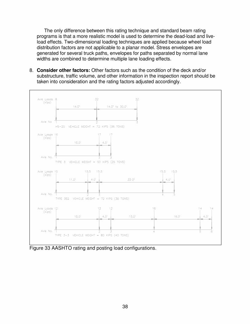
7. Perform load rating: Apply HS-20 and/or other standard design, rating and permit

loads to the calibrated model. Rating and posting load configuration recommended by AASHTO are shown in Figure 33.The same rating equation specified by the AASHTO - Manual for the Condition Evaluation of Bridges is applied:

RF = C - 1A D

2A L(1 + I)

(2)

where: RF = Rating Factor for individual member. C = Member Capacity. D = Dead-Load effect. L = Live-Load effect. A1 = Factor applied to dead-load. A2 = Factor applied to live-load. I = Impact effect, either AASHTO or measured.

38

The only difference between this rating technique and standard beam rating programs is that a more realistic model is used to determine the dead-load and live-load effects. Two-dimensional loading techniques are applied because wheel load distribution factors are not applicable to a planar model. Stress envelopes are generated for several truck paths, envelopes for paths separated by normal lane widths are combined to determine multiple lane loading effects.

8. Consider other factors: Other factors such as the condition of the deck and/or

substructure, traffic volume, and other information in the inspection report should be taken into consideration and the rating factors adjusted accordingly.

Figure 33 AASHTO rating and posting load configurations.

39

Appendix D - References AASHTO (1989). "Standard Specification for Highway Bridges." Washington,D.C. AASHTO, (1994). "Manual for the Condition Evaluation of Bridges", Washington,D.C. Commander,B., (1989). "An Improved Method of Bridge Evaluation: Comparison of Field Test Results with Computer Analysis." Master Thesis, University of Colorado, Boulder, CO. Gerstle, K.H., and Ackroyd,M.H. (1990). "Behavior and Design of Flexibly-Connected Building Frames." Engineering Journal, AISC, 27(1),22-29. Goble,G., Schulz,J., and Commander,B. (1992). "Load Prediction and Structural Response." Final Report, FHWA DTFH61-88-C-00053, University of Colorado, Boulder, CO. Lichtenstein,A.G.(1995). "Bridge Rating Through Nondestructive Load Testing." Technical Report, NCHRP Project 12-28(13)A. Schulz,J.L. (1989). "Development of a Digital Strain Measurement System for Highway Bridge Testing." Masters Thesis, University of Colorado, Boulder, CO. Schulz,J.L. (1993). "In Search of Better Load Ratings." Civil Engineering, ASCE 63(9),62-65.