AD-A110 070 MASSACHUSETTS INST OF TCH CANMNOGE ARTIFICIAL INTl-ETC F/6 17/7

PASSIVE NAVIGATION.IU)NOV 81 A R MUSSP S K MON NO001 S0-C-05osUNCLASSIFIED AI-N-662

NL

Billl

Lm lllll~lffff

Jill I"_. Q8 QILI'

11 1 . 4 1.III uU I'

MICROCOPY RESOLUTION TEST CHARTNATIONAL BUREAU OF STANDARDS 1963-A,

t

I. REPORT NUMBERp GOVT ACCESSION No. RECIPIENT'S CATALOG NUMBER

4. TILE fad SubleS. TYPE Of REPOR & PERIODOCOVERED

. a- ve* Nw'icatiofl S. PERFORMING ORr. REPORT NUBER

7. AUTHOR(&) S. CONTRACT OR GRANT NUNSE101u) -

Anna FRruss and L...lorn

9PERPORM1NG ORrANIZATiO-N NAME AND ADDRESS -W. PROGRAM ELEEN. PROJECT. TASKo Artificial Intelligence Laboratory1-14 545 Technology Square

Cambridge, tassachusetts 02139 _____________

1CONTROLLING OFFICE NAME AND ADDRESS 12. REPORT DATEAdvanced Research Projects Agency14.00 WFlsorn Blvd 13i. NUMBER OF PAGES

-Arlington., Virginia '222051.MONITORING AGENCY NAMIE aAODRESS(I ditift. Item, Ceotp.IIn O1W09) 13. SECURITY CLAS. &Shia tePM,#

Office of Naval Research UNCLASSIFIEDInformationi Systems .

* Arlington.' Virginia 22217 1 15a. 21CLSIFFCATO/DOWMGRAING

IS. DISTRIBUTION STATEMENT (of Sha. Report)

-Distribution of this document Is unlimited.*,Ei3 JAN 26t817. DISTRIDUTON, STATEMENT (Woo* abotra*1 enem.,E s. it.g O 11i lrentfhem. A

to. SUPPLEMENTARY WarnS

None

19. IKY WORCII(Cmu foi's. woe.e*e nD oe O&MYad IWeeIIt by &Iemk nomsma

Passive NavipationopticaliPlbw

C) Tirrc-Varing imagery

I j 20. ASSTRACT (Ceithfo eR faemo. 4140 It 0"060aWY and "a'tty by &i".& oq.Be

- ~ A %4 et'iod is proposed for determinIng the -motion of a body relative to a. f,.xecenvironmnt-itsini the-cliaflina image seen -I a cap'er& attaclied to the I-od.The optical flow in the linage plane is the input, while th~e instantaeous,rotaticn-And trapslatian of thie body are tie output. !tf onti-cp] fl1' couh~e'e etert-ined oreciselv,.. it vioulce only haRVe to '-e 1novin at fewo~ n)Rcoq to com"Outetv- ; 1,rameters of vie r'otinn. in nracticp,'o, t' ''u onotcal "n-,h6 somet:hat inaccurate. Yt is therefore av.artaoeous tr c rs, -- r methiorinf vhiich use as much of the available inforiratlon a- o'~k "e emrnlov a least-

DO ~ 1473 CGISON or I NV ova isus **LT UNCLASSIFIED 0Y'S0S4S0I.-

scniares aroroech 0"'icl rn~ni~'es srcw , mp-sure of t~ie liscrepanc,/v betv4*e-nt.-o ireasured flow land that Tredlctoe froj!, the comnut&ec motion nararoter-.6:"veral differe'nt error norips are 'n--~itiatee. !n 'ofneral, ou' P'lc'oritlrIiads to a systor. of nonlinear ecuat dons f>tom vwhi-c' -o r-I ion naraeter-,mmay be computed numerically. !'owever, in Vi'e s',ecia) cases where Viemotion of the camera is purely translational- or purelv rotational, use ofthe appropriate norm leads to a system of ecuations 4!ro"' vhich tv~ese 'narpr(terscan be determined in closeC' forr.

P -

to1

MASSACHUSETTS INSTITUTE OF TECHNOLOGYARTIFICIAL INTELLIGENCE LABORATORY

A.I. Memo No. M9 November, 1981

PASSIVE NAVIGATION

Anna R. Bruss and Berthold K.P. Horn

/ IAbstract

A method is proposed for determining the motion of a body relative to a fixedenvironment using the changing image seen by a camera attached to the body. Theoptical flow in the image plane is the inpnit, while the instantaneous rotation and trans-lation of the body are the output. If optical flow could be determined precisely, it wouldonly have to be known at a few places to compute the parameters of the motion. Inpractice, however, the measured optical flow will be somewhat inaccurate. It is there-fore advantageous to consider methods which use as much of the available informationas possible. We employ a lcast-squarcs approach which minimizes some measure of thed.:crepancy bctween the measured flow and that predicted from the computed motionparameters. Several different error norms are investigated. In general, our algorithmleads to a system of nonlinear equations from which the motion parameters may becomputed numerically. However, in the special cases where the motion of the camera ispurely translational or purely rotational, use of the appropriate norm leads to a systemof equations from which these parameters can be determined in closed form.

This report describes research done at the Artificial Intelligence Laboratory ofthe Massachuretts Institute of Technology. Support for the laboratory's artificialintlligeii-e research is provided in part by the Advanced lesea;rch Projects Agen'v of

the I )eprtiiient of De'eise. uider Olli-e of Naval IltPetrchl conltract 1O I *l- 8(-C-0505aud in part by Natioual Science Foundation (ranLMCST7-07569.

01 25 82 0911- . -. - -

2

1. Introduction

In this paper we investigate the problem of passive navigation using optical flowinformation. Suppose we are viewing a film. We wish to determine the motion of thecamera from the sequence of images, assuming that the instantaneous velocity of thebrightness patterns, also called the optical flow, is known at each point in the image.Several schemata for computing optical flow have been suggested (e.g. [2], [3], [5]).Other papers (e.g. [9], [10], [11]) have previously addressed the problem of passivenavigation. Three approaches can be taken towards a solution which we term thediscrete, the differential and the continuous approach.

In the discrete approach, information about the movement of brightness patternsat only a few points is used to determine the motion of the camera. In particular, usingsuch an approach, one attempts to identify and match discrete points in a sequence ofimages. Of interest in this case is the photogrammetric problem of determining whatthe minimum number of points is from which the motion can be calculated for a givennumber of images [10], [11], [14]. This approach requires that one tracks features, oridentifies corresponding features in images taken at different times.

In the differential approach, the first and second spatial partial derivatives of theoptical flow are used to compute the motion of a camera [6], [9]. It has been claimedthat it is sufficient to know the optical flow and both its first and second derivativesat a single point to uniquely determine the motion [9]. This is incorrect (except fora special case) [1]. Furthe.more, noise in the measured optical flow is accentuated by )differentiation.

In the continuous approach, the whole optical flow field is used. A major shortcom-ing of both the local and differential approaches is that neither allows for errors in theoptical flow data. This is why we choose the continuous approach and devise a least-squares technique to determine the motion of the camera from the measured opticalflow. The proposed algorithm takes the abundance of available data into account andis robust enough to allow numerical implementation.

2. Technical Prerequisites

In this section we review the equations describing the relation between the motionof a camera and the optical flow generated. We use essentially the same notation as

19]. A camera is assumed to move through a static environment. Let a coordinatesystem X, Y, Z be fixed with respect to the camera, with the Z-axis pointing alongthe optical axis. If we wish, we can think of the environment as moving in relationto this coordinate system. Any rigid body motion can be resolved into two factors,a translation and a rotation. We will denote by T the translational component ofthe motion of the camera and by 0 its angular velocity (see also Figure 1 which isredrawn from [91). Let the instantaneous coordinates of a point P in the environmentbe (X, Y, Z).

aim 2 R

S3y

p U

zw

Figure 1. Coordinate Systems

(Note that Z > 0 for points in front of the imaging system.) Let 7 be the vector(X, Y, Z)T, where T denotes the transpose of a vector, then the velocity of P withrespect to the X,Y, Z coordinate system, is:

S- -T - 0 x(1)

We define the components of P and 0 as:

,( w-(A,B,C)T• (2)

Thus we can rewrite (1) in component form:

X'= -U -- BZ + CY

Y'= -V- CX + AZ (3)Z' = -W -- AY + BX.

where 'denotes differentiation with respect to time.The optical flow at each point in the image plane is the instantaneous velocity of t

the brightness pattern at that point. Let (x, y) denote the coordinates of a point in the~image plane (see Figure 1). Since we assume perspective projection between an object

point P and the corresponding image point p, the coordinates of p are:

'~ C " -

4

x YX Z Y= Y. (4)

The optical flow, denoted by (u, v), at a point (z, y) is:

u = Z' t = I. (5)

Differentiating (4) with respect to time and using (3) we obtain the following equationsfor the optical flow:

X' XZ' U W(6)Y/ YZ' V w

v= +A = (---C -+A-y(--- A-- Bz).

We can write these equations in the form:

U = U, + U. v =v, + v. (7)

where (ut, vt) denotes the translational component of the optical flow and (u,, v,) therotational component:

-- U+zW -V + YWZ Z (8)

u, = Azy - B(z2 + 1) + Cy v, = A(y 2 + 1) - Bzy - Cz.

So far we have considered a single point P. To define the optical flow globally weassume that P lies on a surface defined by a function Z = Z(X, Y) which is positive forall values of X and Y. With any surface and any motion of a camera we can thereforeassociate a certain optical flow and we say that the surface and the motion generatethis optical flow.

Optical flow, therefore, depends upon the six parameters of motion of the cameraand upon the surface whose images are analyzed. Can all these unknowns be uniquelyrecaptured solely from optical flow? The answer is no. To see this, consider a surfaceS2 which is a dilation by a factor k of a surface S,. Further, let two motions denoted byM, and M 2 have the same rotational component and let their translational componentsbe proportional to each other by the same factor k (we will say that M, and M2 aresimilar). Then the optical flow generated by S, and M, is the same as the optical flow

generated by S2 and M 2 . This follows directly from the definition of optical flow (8).It is still an open question whether there are any other pairs of distinct surfaces andmotions which generate the same optical flow.

Determining the motion of a camera from optical flow is much easier if we are toldthat the motion is purely translational or purely rotational. In the next two sectionswe will deal with these two special cases. Then we shall analyze the case where no apriori assumptions about the motion of the camera are made. 0

_______________________________-__

5

3. Translational Case

In this section we discuss the case where the motion of the camera is assumed tobe purely translational. As before, let t = (U, V, W) be the velocity of the camera.Then the following equations hold (see (8)):

Ut = Z V, = Z +(9)z z

3.1. Similar Surfaces and Similar Motions

It will be shown next that if two flows generate the same optical flow, and we knowthat the motions are purely translational, then the two surfaces are similar and the twocamera motions are similar. Let Z, and Z 2 be two surfaces and let 7- (U,, V1, W1 )Tand T2 = (U 2 , V2 , W2 )T define two different motions of a camera, such that Z, and 71,and Z 2 and 12 generate the same optical flow:

-u1 -, W _ V1 W+ YW1 (10)S Z, Z,

-U 2 + zW2 -V 2 + yW 2 (11)Z2 Z2 (1

Eliminating Z1, Z 2 , u and v from these equations we obtain:

-U1 + zW -U 2 + zW-vI + Yw, -v 2 +Yw2 (

We can rewrite this equation as:

(-U - zWI)(-V 2 + yW 2 ) = (-U 2 + zW2)(-VI + yW), (13)I or:

UV 2 -zV 2W, -yUW 2 + zyWW, =2 (UV -zVW 2 -yU 2W, +ZyW2 Wi. (14)

Since we assumed that Z, and T, and Z2 and 1'2 generate the same optical flow, theabove equation must hold for all z and y. Therefore the following equations have tohold:

U1V2 = U2V1-v2W 1 = -V1 W2 (15)

-Uw 2 = -U2w,.

These e uations can be rewritten as:

£ U1:V1:W1 = U2:V2:W2 (16)

II

6

from which it follows that Z2 is a dilation of Zi. It is clear that the scaling factorbetween Z1 and Z2 (or equivalently between I'1 and '2) cannot be recovered from theoptical flow, regardless of the number of points at which the flow is known. By uniquelydetermining the motion of the camera, we will mean that the motion is uniquelydetermined up to a constant scaling factor.

3.2. Least-Squares Formulation

In general, the direction of the optical flow at two points in the image planedetermine the motion of a camera in pure translation uniquely. There is a drawbackhowever to utilizing so little of the available information. The optical flow we measureis corrupted by noise and it is desirable to develop a robust method which takes thisinto account. Thus we suggest using a least-squares method [4], [12] to determine themovement parameters and the surface (i.e., the best fit with respect to some norm).

For the following we assume that the image plane is the rectangle ze[-t, w] andy[-h, h]. The same method applies if the image has some other shape. (In fact, itcan be used on sub-images corresponding to individual objects in the case that theenvironment contains objects which may move relative to one another). Furthermorewe have to assume that 1/Z is a bounded function and that the set of points where 11Zis discontinuous is of measure zero. This condition on 1/Z assures us that all necessaryintegrations can be carried out. We wish to minimize the following expression:

_J__ + (-- YW)z] d (17)

In this case then, we determine the best fit with respect to the ML2 norm which isdefined as:

1I AX, Y) 11= f ij[f(, y)J2dzdy. (18)

The steps in the least-squares method are as follows: First we determine that Z whichminimizes the integrand of (17) at every point (z, y). Then we determine the values ofU, V and W which minimize the integral (17).

Let us introduce the following abbreviations:

a = -U + w f = -v + YW. (19)

Note that the expected flow, given U, V and W is simply:

a P =(20)

Then we can rewrite (17) as:

f J~ (U C )2 + (V - )2]dzTdy. (21) oZ, , (

47

V7

L: u/ - =0

4k(Um 'tM)

Figure 2. Geometrical Interpretation

We proceed now with the first step of our minimization method. Differentiating the

C integrand of (17) with respect to Z and setting the resulting expression equal to zero

yields: ( _ a 3 3(22)Z )- + (V - =F)j2 0. 22

Therefore we can write Z as:~Z - (23)

"a + V'(3

This equation, by the way, imposes a constraint on U, V and W, since Z must bepositive. We do not make use of this except to help us pick amongst two oppositesolutions for the translational velocity later on. Note that now:

Q u __ -vo p - V_ _ _ _ _a

ts v a (24)

Z 2+# C a2 ~ +z2(4

and we can therefore rewrite (17) as:

_W vC +P 2 d (25)

It should be clear, by the way, that uniformly scaling U, V and W does not change

the value of (25). This is a reflection of the fact that we can determine the motion

parame t,!rs only up to a constant factor.Before proceeding with the second step, we give a geometrical interpretation in

£ Figure 2 of what we have so far. Suppose that the motion parameters IT, V, and

,4|

.-- I nn -- M ,

8

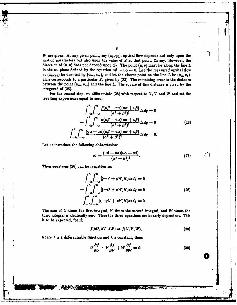
W are given. At any given point, say (Zo, Yo), optical flow depends not only upon themotion parameters but also upon the value of Z at that point, ZO say. However, thedirection of (u, v) does not depend upon Z0 . The point (u, v) must lie along the line Lin the uv-plane defined by the equation u - va = 0. Let the measured optical flowat (zO, yo) be denoted by (ur, v,,), and let the closest point on the line L be (u., v.).This corresponds to a particular Z. given by (23). The remaining error is the distancebetween the point (urn, vin) and the line L. The square of this distance is given by theintegrand of (25).

For the second step, we differentiate (25) with respect to U, V and W and set theresulting expressions equal to sero:

f /i(u/ - vca)(uat + Vft) dzdy = 0

4 f ,~ a(u/i - Va~)(uO + VP) dxdy = 0 (26)

- ,W (a2 + #2)2 vidd -

f ' (ya - zl)(u/3 - va)(ua + VO) dzdy=

Let us introduce the following abbreviation:

K = (up - va)(ua + V"8) (27)(a2 + #2)2

Then equations (26) can be rewritten as:

f hJJf- [(-V + yW)K~dxdy = 0

T'hI [(-U + zW)Kldzdy = 0 (28)

fh [(-yU + xV)Kldzdy = 0.

The sum of U times the first integral, V times the second integral, and W times thethird integral is identically zero. Thus the three equations are linearly dependent. Thisis to be expected, for if:

f(kU, kv, kW) = f(U, V, W), (29)

where f is a differentiable function and k a constant, then:.1

'of af ao (30)U -+ V57V + wY- - .'0

F . . .. -

The result is also consistent with the fact that only two equations are needed, since thetranslational velocity can be determined only up to a constant factor. Unfortunatelyequations (28) are nonlinear in U, V and W and we are not able to show that they havea unique (up to a constant scaling factor) solution.

3.3. Using a Different Norm

There is a way, however, to devise a least-squares method which allows us to displaya closed form solution for the motion parameters. Instead of minimizing (17), we willtry to minimize the following expression:

[(u _ _U + XW) 2 + (V__ - V + YW) 2 1](C2 + 2 )dxdy (31)

obtained by multiplying the integrand of (17) by a2 + #2. Then we apply the sameleast-squares method as before to (31). When the measured optical flow is not corruptedby noise, both (31) and (17) can be made equal to zero by substituting the correct motionparameters. We thus obtain the same solution for the motion parameters whether we

minimize (31) or (17). If the measured optical flow is not exact, then using expression(31) for our minimization, we obtain the best fit with respect not to the ML 2 norm,but to another norm which we call the MLa norm:

*II f(, Y) "= j [f(, y)12(a 2 + 32 )dzdy. (32)

What we have here is a minimization in which the error contributions are weighted,greater importance being given to points where the optical flow velocity is larger. Thisis wost appropriate when the measurement of larger velocities is more accurate.

Which norm gives the best results depends on the properties of the noise in themeasured optical flow. The first norm is better suited to the sitation where the noise inthe measurements is independent of the magnitude of the optical flow. Note also thatif we really want the minimum with respect to the ML 2 norm, we can use the resultsof the minimization with respect to the ML,e norm as starting values in a numericalminimization.

We discuss now our least-squaie" wethod in the case where the norm is chosen tobe ML. . First we determine / by differentiating the integrand of (31) with respectto Z and setting the result equal to zero. We again get (22):

(U -a)e + (- =0o, (33)

from which it follows that (23):

Z - a= +# (34)ua + v#*

7

10

So we want to minimize:

/_f!_ (up - VC) 2dzdy. (35)

Let us call this integral g(U, V, W), then, since:

up - Ver = (vU - uV) - (XV - Yu)W, (36)

we have:

g(U, V, W) = aU2 + bV2 + cW 2 + 2dUV + 2eVW - 2f1WU, (37)

where:

a= f v 2dzdy b = fOhf" . u 2dxdyh W h wu

c = -f (XV - yu)2 dxdY d = - ff uvdxdy (38)h w h --w

C = ThL- u(xv - yu)dxdy f = - ff v(zv - yu)dxdy.

Now g(U, V, W) cannot be negative, and g(U, V, W) = 0 for U = V = W 0. Thusa minimum can be found by inspection, but is not what we might have hoped for. Infact, to determine the translational velocity using our least-squares method we have tosolve the following homogeneous equation for ':

G = o (39)

where G is the matrix:aG= b f

(40)

Clearly (39) has a solution other then zero if and only if the determinant of G is zero.Then the three equations (39) are linearly dependent and T can be determined up toa constant factor. In general, however, as the data is corrupted by noise, g cannot bemade equal to zero for non-zero translational velocity and so P - (0,0, 0)T will be theonly solution to (39). To see this in another way, note that g has the following form:

g(kU, kV, kW) = k'g(U, V, W) (41)

where k is a constant. Clearly g(U, V, W) assumes its minimal value for U = V -W= 0.

What we are really interested in, is determining the direction of P which minimizesg, for a fixed length of 7. Hence we impose the constraint that P be a uitit vector.

A 1 • ' _

S 11

If 1 is constrained to have unit magnitude, the minimum value of g is the smallesteigenvalue of the matrix G and the value of T for which g assumes its minimum can befound by determining the eigenvector corresponding to this eigenvalue [8]. This follows

from the observation that g is a quadratic form which can be written as:

g(U, V, W) = TTGT. (42)

Note that G is a positive semidefinite hermitian matrix as a > 0, b > 0, c > 0, ab >d2 , bc > e2 and ca > f2. (The last three inequalities follow from the Cauchy-Schwarzinequality [7], [8]). Hence all eigenvalues are real and non-negative and are the solutionsX of the third degree polynomial:

X3 - (a + b + c)> 2 + (ab + bc + ca -- d2 - e2 - f 2)X + (43)

(ae2 + bf2 + cd2 - abc - 2def) = 0.

There is an explicit formula for the least positive root in terms of the real and imaginaryparts of the roots of the quadratic resolvent of the cubic. In our case this gives us thedesired smallest root, since the roots cannot be negative. For the sake of completeness,however, various pathological cases that might come up will be discussed next, eventhough they are of little practical interest.

Note that X = 0 is an eigenvalue if and only if G is singular, that is, if the constantterm in the polynomial (43) equals zero. In fact, if the determinant of G is zero one

can find a velocity T which makes g zero. It follows from a theorem in calculus that

this happens only when the optical Bow is either not corrupted by noise at all or only

at a few points. The theorem states that if the integral of the square of a bounded and

cntinuous function is zero then the function itself is zero. Hence errors can only occur

at points where the optical flow is discontinuous, and these are exactly the points where

the surface defined by Z is discontinuous. (These are also the places where existing

methods for computing the optical flow [5] are subject to large errors).It is impossible for exactly two eigenvalues to be zero, since this would imply that

the coefficient of X in the polynomial (43) equalled zero, while the coefficient of X2 did

not. That in turn would imply that ab = d2 , bC = e2 , and ca = f 2, while a, b, andc are not all zero. For equality to hold in the Cauchy-Schwarz inequalities, however,u and v must both be proportional to xv - yu. This can only be true (for all z and

y in the image) if u=v=0. But then all six integrals become zero and consequently

all three eigenvalues are zero. This situation is of little interest, since it occurs only

when the optical flow data is zero everywhere. Then the velocity is zero too. Oncethe smallest eigenvalue is known, it is straightforward to find the translational velocity

which best matches the given data. To determine the eigenvector corresponding to aneigenvalie, say X1, we have to solve the following set of linear equations:

Zap

12

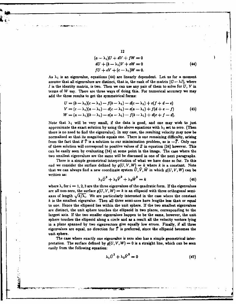
(a - X )U + dV +1W = 0dU + (b - >,)V + eW = 0 (44)fu + eV + (c - X1)W = 0.

As Xi is an eigenvalue, equations (44) are linearly dependent. Let us for a momentassume that all eigenvalues are distinct, that is, the rank of the matrix (G - I), whereI is the identity matrix, is two. Then we can use any pair of them to solve for U, V interms of W say. There are three ways of doing this. For numerical accuracy we mayadd the three results to get the symmetrical forms:

U = (b - ),)(c - X,) - f(b - X1) - d(c - X1) + e(f + d - e)

V = (c - Xi)(a - X) - d(c - XI) - e(a - Xi) + f(d + e - f) (45)

W = (a - X1)(b - Xi) - e(a - X1) - f(b - X1) + d(e + f - d).

Note that X1 will be very small, if the data is good, and one may wish to justapproximate the exact solution by using the above equations with X, set to zero. (Thenthere is no need to find the eigenvalue). In any case, the resulting velocity may now benormalized so that its magnitude equals one. There is one remaining difficulty, arisingfrom the fact that if P is a solution to our minimization problem, so is -P'. Only oneof these solution will correspond to positive values of Z in equation (34) however. Thiscan be easily seen by evaluating (34) at some point in the image. The case where thetwo smallest eigenvalues are the same will be discussed in one of the next paragraphs.

There is a simple geometrical interpretation of what we have done so far. To thisend we consider the surface defined by g(U, V, W = k where k is a constant. Notethat we can always find a new coordinate system U, V, W in which g(U, V, W) can bewritten as:

XlU + X2 +XW = k (46)

where X, for i = 1, 2,3 are the three eigenvalues of the quadratic form. If the eigenvaluesare all non-zero, the surface g(U, V, W) = k is an ellipsoid with three orthogonal semi-axes of length VkVX,. We are particularly interested in the case where the constantk is the smallest eigenvaue. Then all three semi-axes have lengths less than or equalto one. Hence the ellipsoid lies within the unit sphere. If the two smallest eigenvaluesare distinct, the unit sphere touches the ellipsoid in two places, corresponding to thelargest axis. If the two smaller eigenvalues happen to be the same, however, the unitsphere touches the ellipsoid along a circle and as a result all the velocity vectors lyingin a plane spanned by two eigenvectors give equally low errors. Finally, if all threeeigenvalues are equal, no direction for P is preferred, since the ellipsoid becomes theunit sphere.

The case where exactly one eigenvalue is zero also has a simple geometrical inter-pretation. The surface defined by g(U, V, W) = 0 is a straight line, which can be seeneasily from the following equation:

\I &2 + X 2 0 0 (47)

* 13

written for the case when X3 is zero. (Remember that X1 and X2 are both positive.)Clearly the unit sphere intersects this line in exactly two points, one of them cor-responding to positive values for Z in equation (34).

The method which we just described can be easily implemented. To this end, theproblem can be discretized. An expression similar to (31) can be derived where theintegrals are approximated by sums. Our minimization method can then be appliedto these sums. The resulting equations are similar to ones described in this section,with summation replacing integration. We implemented the resulting algorithm andtested it using synthetic data including additive noise. Thes results agreed with ourexpectations.

One can use the ratio of the biggest to the smallest eigenvalue, the so calledcondition number [13], as a measure of confidence in the computed velocity. The resultis very sensitive to errors in the measurements unless this ratio is much bigger thanone.

Curiously, the same error integral as (35) is obtained in the case where the MLz..norm is used:

hlz =/ [f(Xy)Z(Xy)1 2(u' + v2)dzdy. (48)

We can arrive at a similar solution by multiplying the integrand in (17) by Z2 insteadof by a2 + . In that case the minimization is carried out with respect to the MLznorm defined by:

II f(x, f') [z _ f(, y)Z(, )]2dzdy. (49)

Here optical flow velocities for points which are further away are weighted more heavily.This is most appropriate when the measurement of larger velocities is less accurate.We end up with a quadratic form similar to g, only the integrals for the six constantscorresponding to a, b, c, d, e, and f are a bit more complicated. Curiously they onlydepend on the direction of the optical flow at each point, not its magnitude.

Also, other constraints could be used. If we insist on U2 + V 2 = 1, for example, weobtain a quadratic instead of a cubic equation, and if we use W = 1, a linear equationonly need to be solved. The disadvantage of these approaches is that the result issensitive to the orientation of the coordinate axes. Clearly, in the case of exact data,we get the right solution using any of the constraints mentioned above.

34. Using a Different Constraint

The minimization scheme discussed in the previous section gives us a uniquesolution in most cases for the velocity vector t. Here we propose a slightly differentapproach which always gives us a unique solution. Note that applying the first step inour minimization method gives us a constraint between the values of Z, the velocity

'1 ," T .

14

vector and the optical flow at every point. We can in addition ssume that Z = Zo isknown at a particular point, say (Zo, yo). Using the MLz, norm in our scheme, wewant to minimize:

[UZ _ (-U + zW)J, + [vZ _ (-V + YW)J 2(U + ti)dzdy. (50)

Differentiating (50) with respect to Z, and setting the resulting expression equal to zero,we obtain:

U2 + V2 51

Thus we propose to solve the minimization scheme under the following constraint:

Zo(U + V2) - (Uo0 + Vop) = 0 (52)

where uo and vo denote the components of the optical flow measured at (Zo, yo). Theerror integral (50) becomes after substituting (51):

_ji (Up - VI)2dZdy (53)

which is the same as (35) and is denoted by g(U, V, W) (37). Thus we want to minimize: ' )

g(U, V, W) + 2X[Zo(uo + v0) - (uoa + von)] (54)

where X denotes a Lagrangian multiplier. To determine U, V and W the followinglinear equations obtained by differentiating (54) with respect to U, V, W and X have tobe solved:

aU + dV +W+ Xuo - 0

dU + bV + eW + Xvo 0 (55)f U + eV + cW - X(zoUo + poao) =" 0UoU + VOV - (ZoUo + ioVo)W = -Zo(O + Vo).

These equations can be written in the form:

,, =F (56)

where a P ( = (U, V, W, X)T and 2 (0,0,0, -Z0(t4 + v2))T. Let the determinant ofCX be A0:

A0 =(d' - ab)(zouo + YoVo) 2 + (e' - bc)uo + (f2 - ac)v -+ (57)2[(de - bf )uo(zouo + yovo) + (df - ae)vo(zouo + Yovo) + (cd - ef)uovo]. 0 "I

• - 0-

AhI

0 15Assuming that A0 3 0 we can easily determine 'x from (55):

GX -. (58)

Introducing the following abbreviation:K-- Z0(i4' + t4)()

AO (5)

we can give these formulae for '),:

U = K[uo(bc - e') + vo(ef - cd) + (ZoUo + yovo)(bf - de)]

V = K[uo(ef - cd) + vo(ac - f2) + (ZoUo + yovo)(ae - df)] (60)

W = K[uo(de - bi) + vo(df - as) + (z0t 0 + yovo)(d 2 - ab)]

X = K[ae2 + d2 + bf 2- abc - 2def].

The disadvantage of this approach is that the result depends upon the values of theoptical flow at a single point. To circumvent this problem we propose to determineaverage values for U, V and W in the following manner. First note that we are onlyinterested in the ratios of U/W and V/W which obviously do not depend upon the(unknown) value for Zo. Equivalently we could determine the value for K from thecondition that 7 should have unit length. Hence we can determine values for U, Vand W which depend only upon the values of the optical flow at a sing!e point and thecoefficient in the matrix G. If we want to remove the dependence of the result on thedata at a single point, we can simply average the values obtained for all image points.

In the case where the data is exact, i.e., where the determinant of G, denotedby detG, vanishes, the solution for T is the same one as obtained using no constraintin our minimizations scheme. To see this just observe that in that case X = 0 asX = -KdetG). In the case where AO = 0, equations (55) have a solution only whendetG = 0. We do not have to be concerned with the case where A0 = 0 but detG 3 0as we can argue that equations (55) always have to have a solution. Note that ourmethod is based on the condition that Z is a certain function (51) of U, V, W. Hence(52) cannot impose a constraint which would be impossible to satisfy.

4. Rotational Case

Suppose now that the motion of the camera is purely rotational. In order todetermine the motion from optical flow we again use a least-squares algorithm with theML 2 norm described in the previous section. Recall that in this case the optical flowis (see (8)):

u, = Axy - B(z2 + 1) + Cy (61)

*v, = A(y' + 1) - Bxy - Cx.

IblMW NNW%" .

16

We will show now in an analogous fashion to section 3.1 that two different rotations,

say 0D = (Ai, Bi, Ci)T and 02 = (A2 , B 2, C2 )T, cannot generate the same optical flow.Assuming the converse, the following equations have to hold for all values of z and y:

Aixy - Bi(x2 + 1) + Ciy = A2Xy - B2(X2 + 1) + C¢y (62)

AI(y 2 + 1) - Bixy - Cx = A 2(y' + 1) - B 2zy - C 2 z

from which we can immediately deduce that 0i = 02.

In general, the direction of the optical flow at two points and its magnitude at one

point determine the motion of a camera in pure rotation uniquely. We choose insteadto minimize the following expression:

_ _ [(U -- U,)2 -+- (V -- V,)2dd. (63)

As the motion is purely rotational, the optical flow does not depend upon the distanceto the surface and therefore we may omit the first step in our method. Thus we imn-

mediately differentiate (63) with respect to A, B and C and set the resulting expressionsequal to sero:

h f K(U - U,)Ty + (V - V,)(y 2 + )I)dzdi = 0

hf [(u - u,)(z2 + 1) + (v - v,)zy]dzdy = 0 (64)

f . I - u,)y - (v - v,)xldxdy = 0.

Rewriting the above equations we obtain:

f;f [uzy + v( = + - 1)]dxdp =-- _ [u,zy + V,(y2 + 1)]dZdyh W h w

hf [U(z + 1) + vxyldzdy = .U,(Z + 1) + Vit]dy (65)h w h W

and expanding these equations yields:

AA +2B +7C==k2A + + 2C --- (66)7A + 2B + Zc =M,

Okt

0 17

where:

h W

W[~2+ (y2 + F]dd

= f-f__[(z2 + 1)2 + X2y'Jdzdy

=L f__[W +pJd (67)

aT = - Jhf: 2 + y2 + 2)]dxdy

h W

ydxdy7 = f T e- ]dzdy,

and:

= h- [uXy + V(y2 + 1)]dzdyh W

1= i- i-u1_ ' J 2 + 1)v + v]x d z(68)h W

If we call the coefficient matrix in (66) M and the column vector on the right-hand sideR4, then we have:

MQ = ft. (69)

Thus, provided the matrix M is non-singular, we can compute the rotation as follows:

a - M - 1 . (70)

It is easy to see that the matrix M is non-singular in the special case of a rectangular

image plane since then:h' 2h' 4tuShs

A4wh( + " + 4w+

4wh,!--l + hs) (71

4wh 2 h23 (

77 a-RUN=0.

[i ~ ~.....

So in the case of a rectangular image plane, the matrix is diagonal, which makes itparticularly easy to compute its inverse. In fact, the matrix is diagonal if the imageplane is symmetrical about the z-axis and the y-axis. As the extent of the image planedecreases, however, the matrix M becomes ill conditioned. That is inaccuracies in thethree integrals (E, 1, and M) computed from the observed flow are greatly magnified.This makes sense since we cannot expect to accurately determine the component ofrotation about the optical axis when observations are confined to a small cone ofdirections about the optical axis. Again, in our numerical implementation of thealgorithm the integrals in (67) can be approximated by sums.

5. General Motion

We would like now to apply a least-squares algorithm to determine the motion of acamera from optical flow given no a priori assumptions about the motion. It is plain thata least-squares method is easiest to use when the resulting equations are linear in all themotion parameters. Unfortunately, there exists no norm which will allow us to achievethis goal. We did find a norm, however, which resulted in equations that are linear insome of the unknowns and quadratic in the others. We again attack the minimizationproblem using the MLap norm under the constraint that U2 + V 2 + W2 = 1. Theensueing equations are polynomials in the unknowns U, V, W, A, B and C and can besolved by a standard iteration method like Newton's method or Bairstow's method [12]or by an interpolation scheme like regula falsi 112]. The expression we wish to minimizeis: /2# °

f - ( - t,) + [V + ,)]l}(g2 + #2)dZdy. (72)

The first step is to differentiate the integrand of (72) with respect to Z and set theresulting expression equal to sera:

Z a2~= + #2 73( ,)O + (V - (73)

We introduce the Langrangian multiplier X as before and attempt to minimise:

JJ (U - U,)#- (V - V,)aIddy + A(U2 + V 2 + W2 - 1). (74)

The equations we have to solve to determine the motion parameters are obtained by ()

7--,

!• -t S

differentiation-

_hfJ (U - (v - v,)][(z 2 - 1) ]dxdy = 0

T __(u - U,)# - -(v - [ 1)p _ zadzdy = 0

h' ,.[(u- u )# - (v - v,)alJ[Y + x U]dxdy = 0 (T5)

J [(u - - (V - Vr)av, dzdy + XU = 0/' _- )# - . ( - -),c.)au,+.dzdy + XV = 0

U2 "- V 2 = 1.

Note that the first three of thee equations are linear in A, B and C from which theseparameters can be determined uniquely in terms of U, V and W. Then we can determineU,V and W from the last four equations by a numerical method. To this end, theproblem can be discretized and equations analogous to (75) derived, where summationof the appropriate expressions is used instead of integration.

6. Summary

Our objective was to devise a method for determining the motion of a camera fromoptical flow which allows for noise in the measured data. The least-squares methodwhich we proposed in this paper meets our goal and is also suitable for numericalimplementation. An important application of our results is in passive navigation. Herethe path and instantaneous altitude .of a vehicle is to be determined from informationgleaned about the environment without the emission of sampling radiation from thevehicle.

Acknowledgement*: The first author wants to thank Stephen Trilling for helpful com-ments which improved the style of this paper. We also want to thank Judi Jones formaking the drawings.

7. Roferences

11) Brus. A.R., "Counterexample," unpublished manuscript, (1981).

7jr

* -- .a .. .'.-,r... -,- t.''.. i | . : --- a

20

[2] Fennema C.I. and Thompson W.B., "Velocity Determination in Scenes Containing 3Several Moving Objects," Computer Graphics and Image Processing Vol. 9, No.4, (1979), 301-315.

13] Hadani I., Ishai G. and Gur M., "Visual Stability and Space Perception inMonocular Vision: Mathematical Model," Journal of the Optical Society ofAmerica Vol. 70, No. 1, (1980), 60-65.

14] Hildebrand F.B., Introduction to Numerical Analysis, McGraw-Hill, (1974).

[5] Horn B.K.P. and Schunk B.G., "Determining Optical Flow," Artificial IntelligenceVol. 16, No. 1-3, (1981), 185-203.

[6] Koendrink J.J. and van Doom A.J., "Local Structure of Movement Parallax ofthe Plane," J. Opt. Soc. Am. Vol. 66, No. 7, (1976), 717-723.

[7] Kolmogorov A.N. and Fomin S.V., Introductory Real Analysis, Prentice-HallInc., (1970).

[81 Komn G.A. and Korn T.M., Mathematical Handbook for Scientists and Engineers,McGraw-Hill Book Co., (1968).

[9] Longuet-Higgins H.C. and Praidny K., "The Interpretation of a Moving RetinalImage," Proc. Roy. Soc., Vol. B, No. 208, London, (1980), 358-397.

[10] Meiri A.Z., "On Monocular Perception of 3-D Moving Object," IEEE Transactionson Pattern Analysis and Machine Intelligence Vol. PAM[-2, No. 6, November(1980), 582-583.

[11] Nagel H.-H., "On the Derivation of 3D Rigid Point Configurations from Image

Sequences," EEE Conference on Pattern Recognition and Image Processing(1981).

[12] Stoer J. and Bulirsch R., Introduction to Numerical Analysis, Springer-Verlag,(1980).

113] Strang G., Linear Algebra and its Applications, Academic Press, (1976).

114] .Ullman S., The Interpretation of Visual Motion, The MIT Press, (1979).

-i

DAT

ITI

Ilk