Living with Hogs in Iowa: The Impact of Livestock ... · Living with Hogs in Iowa: The Impact of Livestock Facilities on Rural Residential Property Values Joseph A. Herriges, Silvia

Living with Hogs in Iowa: The Impact of Livestock Facilities on Rural Residential Property Values

Joseph A. Herriges, Silvia Secchi, and Bruce A. Babcock

Working Paper 03-WP 342 August 2003

Center for Agricultural and Rural Development Iowa State University

Ames, Iowa 50011-1070 www.card.iastate.edu

Joseph Herriges is a professor of economics; Silvia Secchi is an assistant scientist with the Resource and Environmental Policy Division, Center for Agricultural and Rural Development (CARD); and Bruce Babcock is a professor of economics and director of CARD; all at Iowa State University. The authors thank Ivaylo Minkov and Yongsik Jeon for their excellent research assistance, and the assessor’s offices of Franklin, Hamilton, Hardin, Humboldt, and Webster counties for their help in gathering data. This publication is available online on the CARD website: www.card.iastate.edu. Permission is granted to reproduce this information with appropriate attribution to the authors and the Center for Agricultural and Rural Development, Iowa State University, Ames, Iowa 50011-1070. For questions or comments about the contents of this paper, please contact Joseph Herriges, 369 Heady Hall, Iowa State University, Ames, IA 50011-1070; Ph: 515-294-4964; Fax: 515-294-0221; E-mail: [email protected]. Iowa State University does not discriminate on the basis of race, color, age, religion, national origin, sexual orientation, sex, marital status, disability, or status as a U.S. Vietnam Era Veteran. Any persons having inquiries concerning this may contact the Director of Equal Opportunity and Diversity, 1350 Beardshear Hall, 515-294-7612.

Abstract

To better understand the magnitude of the effects of livestock feeding operations on

residential property values, we constructed a new dataset that merges data on home sales

with data on the location and size of livestock feeding operations in five rural counties of

Iowa. We estimated a hedonic model to explain variations in residential sales price with

standard house attributes, such as number of bedrooms and square feet of living space, as

well as the effects of distance and density of livestock feeding operation. We find that

livestock operations have an overall statistically significant effect on property values.

Predicted negative effects are largest for properties that are downwind and close to

livestock operations. In addition, feeding operations that are moderate in size have more

impact than do large-scale operations, most likely reflecting age, type, and management

practices of the moderate-sized operations. The limited size of the estimated effects

suggest that common sense rules—such as not locating feeding operations close to and

upwind of residences—combined with modest compensatory payments could help rural

residences co-exist with modern feeding operations.

Keywords: hedonic model, livestock, property values.

LIVING WITH HOGS IN IOWA: THE IMPACT OF LIVESTOCK FACILITIES ON RURAL RESIDENTIAL PROPERTY VALUES

Introduction The methods used to raise hogs in Iowa have undergone dramatic changes in the past

twenty years. In 1980, approximately 65,000 farmers in the state raised hogs, with an

average of 200 hogs residing on each farm. In 2002, the number of farms with hogs had

fallen to about 10,000, and the average number of hogs per farm had risen to over 1,400.1

In the not-so-distant past, the presence of livestock on farms was the norm. When living

or traveling in rural areas, one expected to smell the smells, hear the noises, and see the

sights that accompany such operations. Complaints between rural neighbors about

livestock operations made little sense when everybody had livestock. But the dramatic

increase in the concentration of ownership now means that far fewer rural residents have

a large financial interest in livestock. What once was the smell of money is now the smell

of somebody else’s money and an externality to be dealt with. Moreover, there is a

concern that the increased concentration of the industry may be accompanied by an

increased risk of environmental damage due to manure spills and further degradation of

local air quality as the result of odor emanating from large-scale hog facilities.

Accompanying the changes in the industry’s structure has been an increase in

complaints about livestock operations. State and local agencies have responded by

enacting regulations for large-scale confinement units. Since 1995, the Iowa legislature

has passed three progressively stricter bills regulating livestock operations. The most

recent bill, Senate File 2293, provides for a lower size threshold at which a construction

permit is required, calls for larger separation distances for livestock operations, and

regulates air quality by limiting emissions from confinement operations.2 In addition to

such legislative action, since the Iowa Supreme Court in 1998 limited the immunity

granted to farmers raising livestock, there have been several instances in which individual

landowners have filed lawsuits against hog facilities. The best-known case involves four

farm couples—two of whom had raised livestock—who sued Iowa Select Farms in 2002

2 / Herriges, Secchi, and Babcock

for the production of offensive odors, noxious gasses, and excessive flies on the

company’s 30,000-head hog facility in Sac County, Iowa. The plaintiffs were awarded

$1.06 million in actual damages plus $32 million in punitive damages.3 The case was

settled out of court in 2003, but the terms of the settlement are confidential.

The problem facing both regulators and the judicial system is that little information

exists on the extent of damages caused by livestock facilities, making regulation and

assessment of damages in civil suits that much more difficult. Palmquist, Roka, and

Vukina 1997 (PRV hereafter) represents one of the few studies available. Using data on

237 rural residential properties in southeastern North Carolina, PRV conducted a hedonic

price analysis. The authors found that proximity to hog facilities caused a statistically

significant reduction in rural housing prices, with an impact of as much as 9 percent for a

facility located within ½ mile of a home. A limitation of the PRV study is that the authors

did not have information on the exact location of the hog operations. Instead, the authors

were forced to rely on an index of manure production within three radii of each home sale

(0 to ½ mile, ½ to 1 mile, and 1 to 2 miles) provided by the state veterinarian’s office.

This precluded the authors from controlling for whether facilities were upwind or

downwind of the residential site or the specific distance to the nearest facility. Moreover,

the authors did not control for the potentially positive impact that growth in the local

livestock industry might have on the demand for housing in the region.

The purpose of this paper is to address some of the limitations inherent in data

available for the PRV study by using GIS (geographical information systems) data on the

location of livestock facilities in Iowa. Specifically, we conducted a hedonic analysis of

the impact of livestock facilities on rural residential property values. We collected data on

1,145 actual home sales in five counties (Franklin, Hamilton, Hardin, Humboldt, and

Webster) for the period from 1992 through the summer of 2002. We merged these data

with information from the Iowa Department of Natural Resources (IDNR) on the location

and size of livestock operations requiring either a construction permit or a manure

management plan to determine how close each home was to livestock facilities. The

livestock operations database used in the analysis includes facilities regulated according

to the 1998 law, House File 2494, which required operations with an animal weight

capacity in excess of 200,000 pounds (400,000 for bovine facilities) to file a manure

Living with Hogs in Iowa: The Impact of Livestock Facilities on Rural Residential Property Values / 3

management plan. Construction permits were required for facilities over 625,000 pounds

of bodyweight (roughly 4,167 finishing hogs) that used formed storage.4 For each

residence, we identified the nearest livestock operation, recording the operation’s

distance from the home, its size (live weight), and whether it was upwind of the home

during the winter (i.e., northwest) or summer (i.e., south) seasons. We also computed the

number of operations within a 3- and 10-mile radius to control for concentration effects

and the indirect impact of industry growth on housing demand.

Literature Review Hedonic price models have long been used to value not only the physical attributes

of housing units (e.g., square footage, number of bathrooms, and air conditioning) but

also the surrounding location and environmental amenities (e.g., local school quality,

crime rates, and air quality).5 Drawing on seminal work by Rosen (1974), hedonic

property value studies start with the notion that the price of a home ( P ) reflects the

bundle of attributes associated with it; that is,

( )1 2, , , KP P z z z= … (1)

where ( )1 2, , , Kz z z= …z is a vector of housing attributes. The hedonic function in

equation (1) is a housing market equilibrium resulting from the interplay between

consumers’ demands for various bundles of attributes and suppliers’ costs of providing

such bundles. As such, it can be used to value marginal changes in a given attribute

(say, kz ) using

( ) ( )k

k

PMV

z∂

=∂

zz . (2)

However, one must be careful in using the hedonic function to measure large (i.e., non-

marginal) changes in the set of housing amenities, as this may result in a change in the

market equilibrium. According to PRV (p. 115), if the changes are localized (and hence

not likely to alter substantially the local housing market), the hedonic function can be


used to value changes in local environmental amenities. Moreover, they argue that this is

likely to be the case in considering the impact of locating a new hog facility.

The empirical literature that employs hedonic analysis to value environmental

amenities is substantial in both the size and scope of amenities being valued. For

example, Smith and Huang (1995) use meta-analysis to summarize nearly 40 studies of

the impact of air quality on housing prices. Perhaps more relevant to the current analysis

are those studies focused on Locally Undesirable Land Uses (or LULUs), including

landfills, hazardous waste sites, and incinerators.6 For example, Kohlhase (1991), Kiel

(1995), McCluskey and Rausser (2001), and Smith and Desvousges (1986) all estimate

the impact of hazardous waste sites on residential property values and typically find that

home values are significantly reduced by proximity to such disposal sites. Similar results

emerge in studying the impact of incinerator sites (Kiel and McClain 1995a,b) and

landfills (Thayer, Albers, and Rahmatian 1992; Reichert, Small, and Mohanty 1992).

As previously noted, however, there are relatively few studies that focus on the

impact of livestock facilities on property values, with PRV being perhaps the most well-

known to date. An earlier hedonic analysis by Abeles-Allison and Conner (1990) also

found a significant impact of hog facilities on property values in Michigan. However, the

analysis was subject to potential sample selection bias, as properties studied were limited

to those located near hog facilities for which multiple complaints had been received. Taff,

Tiffany, and Weisberg (1996) and Mubarak, Johnson, and Miller (1999) conducted

property value studies in Minnesota and Missouri, respectively, but were hampered by

limited information on the characteristics of the properties being sold. Moreover, in the

Missouri study, over 60 percent of the parcels did not include a home; those that did

include a home did not control for the homes’ structural characteristics. The Minnesota

study, on the other hand, used only house sales data but included property located in

cities or townships with populations of 2,500 people or less. It therefore did not

distinguish between rural and urban sales, and it had very little information on the

characteristics of the properties sold.7 To our knowledge, the only other hedonic study

that controls for the presence of livestock facilities is a recent paper by Ready and

Abdalla (2003), which analyzes single-family home sales in Berks County, Pennsylvania.

In this study, the authors estimate a hedonic price function, including as housing


amenities the proximity of each home to open space and disamenities, such as landfills,

regional airports, and large animal production facilities. The authors find that a large

animal production facility located at a distance of 500 meters (or roughly 0.3 miles)

depresses the sales price of a home by 6.4 percent. However, the authors do not control

for the direction of the housing unit relative to the livestock facility.

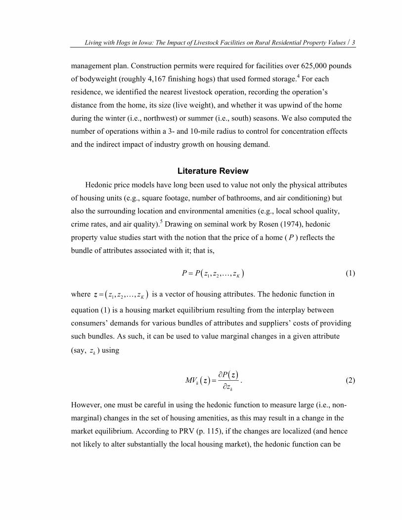
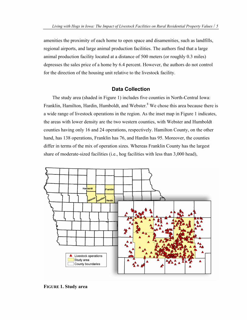
Data Collection The study area (shaded in Figure 1) includes five counties in North-Central Iowa:

Franklin, Hamilton, Hardin, Humboldt, and Webster.8 We chose this area because there is

a wide range of livestock operations in the region. As the inset map in Figure 1 indicates,

the areas with lower density are the two western counties, with Webster and Humboldt

counties having only 16 and 24 operations, respectively. Hamilton County, on the other

hand, has 138 operations, Franklin has 76, and Hardin has 95. Moreover, the counties

differ in terms of the mix of operation sizes. Whereas Franklin County has the largest

share of moderate-sized facilities (i.e., hog facilities with less than 3,000 head),

FIGURE 1. Study area


Hamilton County has the greatest number of larger facilities (i.e., over 3,000 head).9 Over

90 percent of the facilities are hog operations, mostly growers, and the majority of them

were built in the early to mid-1990s.

Livestock Facilities Data Information on each livestock facility in the study area was obtained from the IDNR.

The available data included the GIS files on the location of the operations as well as the

live weight and animal type in production. We identified two types of operations using

the IDNR data: facilities that need a construction permit and facilities that need to file a

manure management plan with the agency. In general, according to the 1998 Iowa law,

any operation with an animal weight capacity of more than 200,000 pounds (400,000

pounds bovine) must obtain a manure management permit. If a facility uses earthen

storage structures for manure, such as a lagoon, it must also obtain a construction permit.

If a facility uses formed storage, on the other hand, it needs a construction permit only for

operations with 625,000 or more of animal weight capacity (1.6 million pounds or more

for bovine).

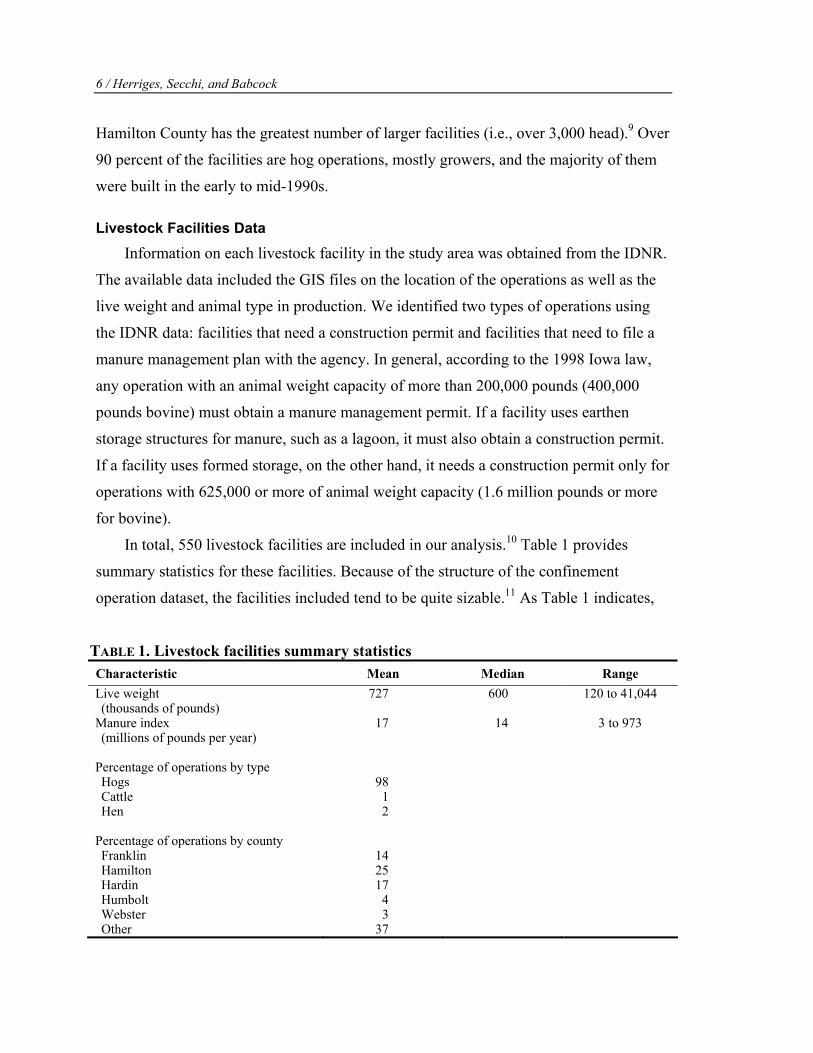
In total, 550 livestock facilities are included in our analysis.10 Table 1 provides

summary statistics for these facilities. Because of the structure of the confinement

operation dataset, the facilities included tend to be quite sizable.11 As Table 1 indicates,

TABLE 1. Livestock facilities summary statistics Characteristic Mean Median Range Live weight (thousands of pounds)

727 600 120 to 41,044

Manure index (millions of pounds per year)

17 14 3 to 973

Percentage of operations by type Hogs 98 Cattle 1 Hen 2

Percentage of operations by county Franklin 14 Hamilton 25 Hardin 17 Humbolt 4 Webster 3 Other 37


their live weight ranges from 120,000 to 41,044,000 pounds, with a median of 600,000

and an average of 727,000.12 Over 97 percent of the facilities are hog confinement units,

1 percent are cattle operations, and the remaining 2 percent are egg laying facilities.

In order to provide some comparability to PRV, we also considered manure

production as an alternative measure of size in our hedonic analysis. A manure index was

formed for each facility based on type of facility and using the algorithms developed by

Lorimor, Powers, and Sutton (2000). Manure production levels, as excreted, for facilities

included in the study ranged from 3 to 973 million pounds per year, with a median and

mean, respectively, of 14 and 17 million pounds per year.

Residential Property Sales Data Data on house sales were obtained from each county assessor’s office. We restricted

sales to rural residential, owner-occupied homes sold via “arms length” transactions

between 1992 and 2002.13 As in the case of PRV, we excluded properties with more than

10 acres in order to avoid units that were being marketed in part because of their

agricultural production capabilities. We also excluded properties whose sale prices were

less than 50 percent of their assessed values and/or sold for less than $5,000. In total,

1,145 sales were available for the analysis. Table 2 details the number of sales and

earliest sale date by county.

The variables used in the hedonic regression analysis fall into three broad categories:

(a) the physical attributes of the home and lot (e.g., square footage and number of

bathrooms), (b) the attributes of the surrounding community, and (c) the attributes of the

livestock facilities in close proximity to each home. The physical characteristics available

for each home varied by county. In total, 11 characteristic were formed using the overlap

in information across the five counties, including the size of the lot, the age of the home,

TABLE 2. Rural residential property sales by county County Earliest Sales Date Number of Sales Franklin January 1993 141 Hamilton January 1992 190 Hardin January 1995 177 Humboldt March 1995 71 Webster January 1992 566


and the year in which it was sold, the size of the living area and any additions to the

home, and the number of bathrooms, decks and fireplaces. These characteristics, listed in

the first part of Table 3, are similar to those used in PRV and other hedonic studies of

residential properties. Each of these characteristics, with the exception of the age of the

home, is expected to have a positive impact on the price of the home.

The second broad category of explanatory variables (listed in the second section of

Table 3) characterizes the amenities of the housing unit in terms of the surrounding

community. These include the distance to the nearest large town (i.e., with population of

2,500 or more) and nearest high school, as well as the median income and population

density for the corresponding township. The two distance variables required locating each

household spatially. For two counties, Webster and Hardin, GIS files with parcel

locations were available. For the other three, we used Digital Orthophoto Quarter Quads

(DOQQs) of the State of Iowa combined with paper or online maps to create the GIS data

layers.14,15 An application called PCMiler was then used to calculate the distance from

each home to both the local high school and the closest town with a population of more

that 2,500 within the 10-mile buffer.16 In general, we expected that an increase in either

of these distances would negatively affect a home’s sale price.

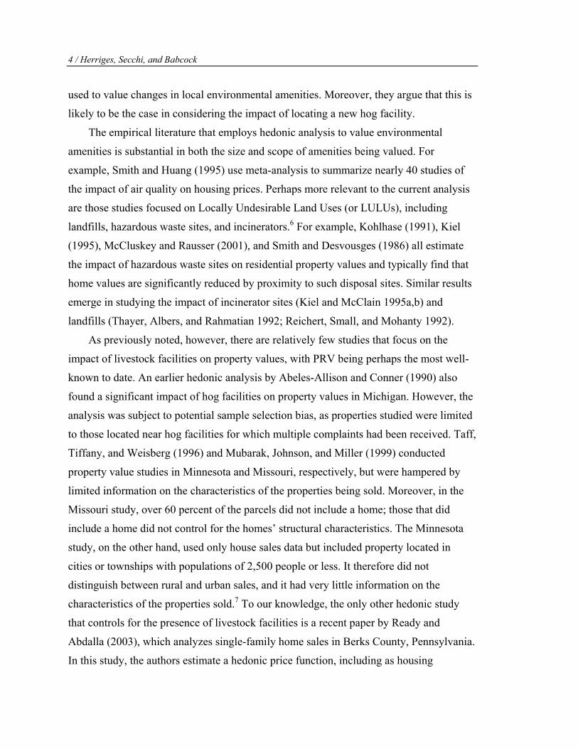
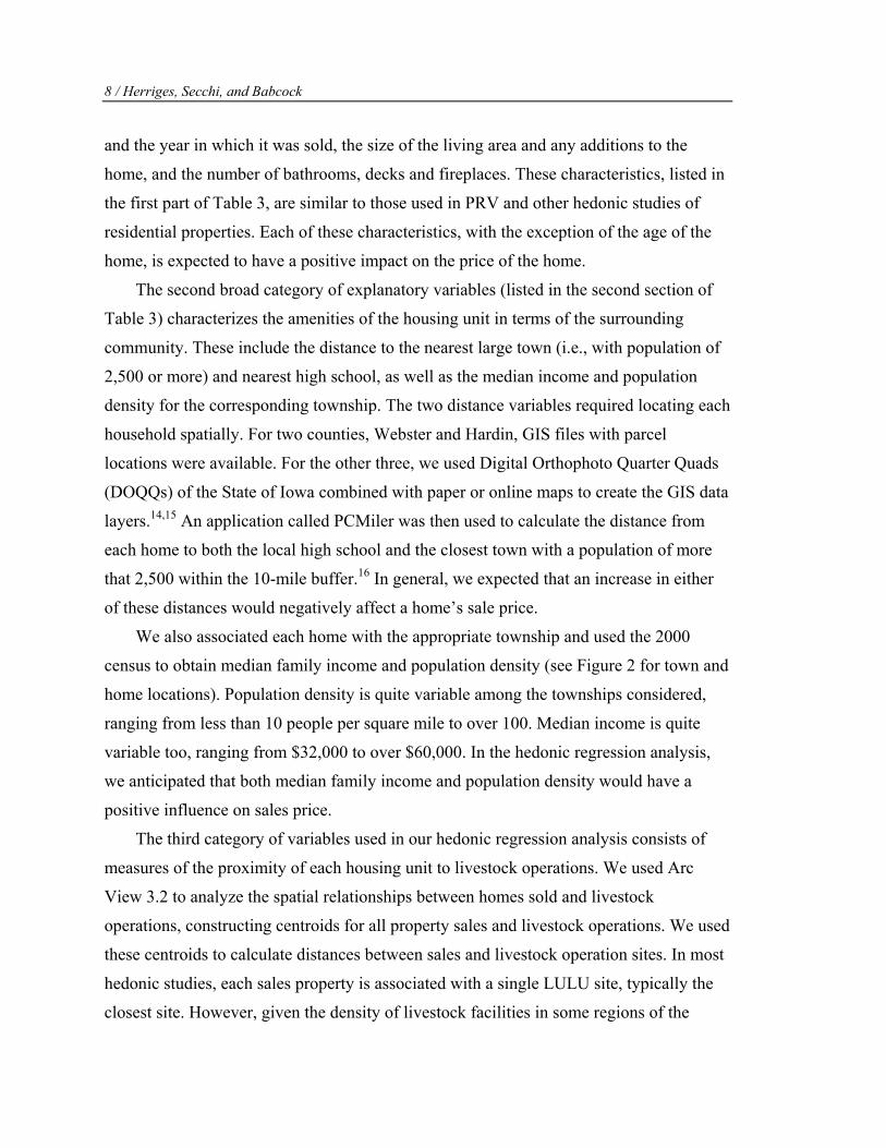
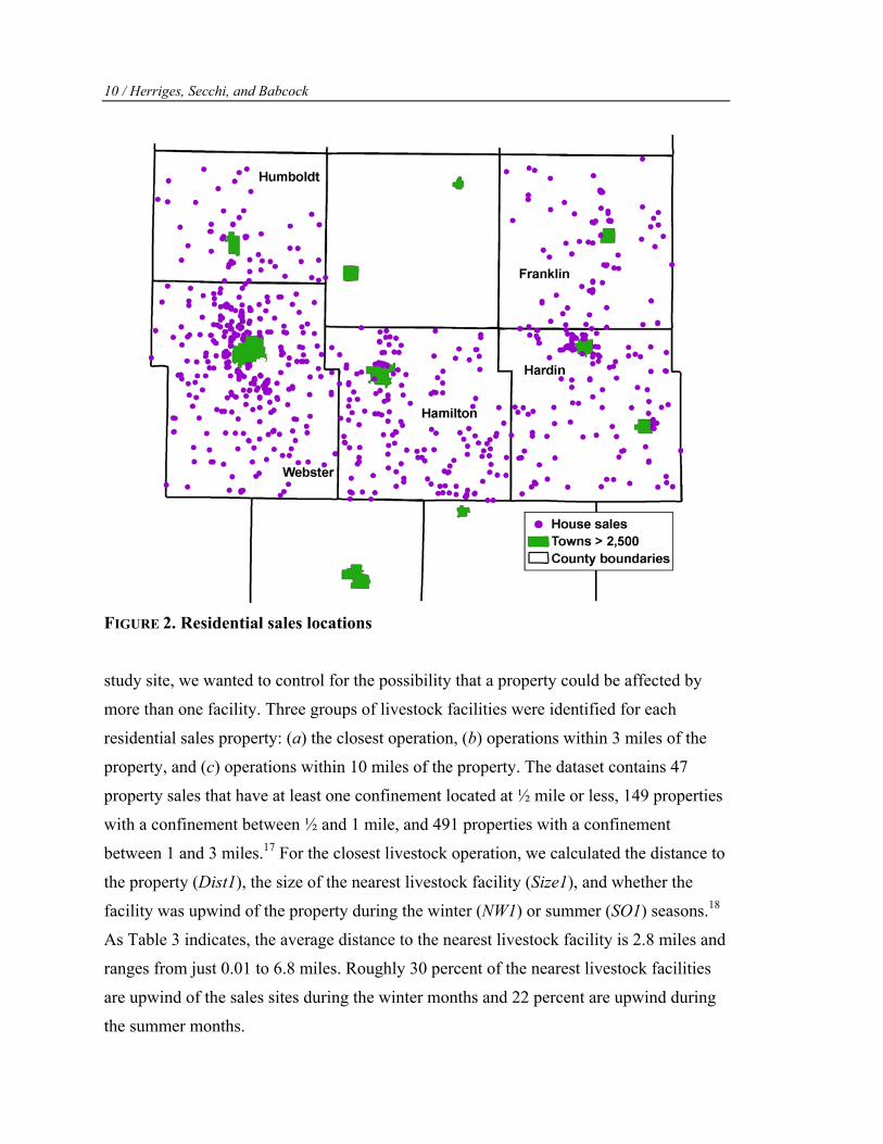
We also associated each home with the appropriate township and used the 2000

census to obtain median family income and population density (see Figure 2 for town and

home locations). Population density is quite variable among the townships considered,

ranging from less than 10 people per square mile to over 100. Median income is quite

variable too, ranging from $32,000 to over $60,000. In the hedonic regression analysis,

we anticipated that both median family income and population density would have a

positive influence on sales price.

The third category of variables used in our hedonic regression analysis consists of

measures of the proximity of each housing unit to livestock operations. We used Arc

View 3.2 to analyze the spatial relationships between homes sold and livestock

operations, constructing centroids for all property sales and livestock operations. We used

these centroids to calculate distances between sales and livestock operation sites. In most

hedonic studies, each sales property is associated with a single LULU site, typically the

closest site. However, given the density of livestock facilities in some regions of the

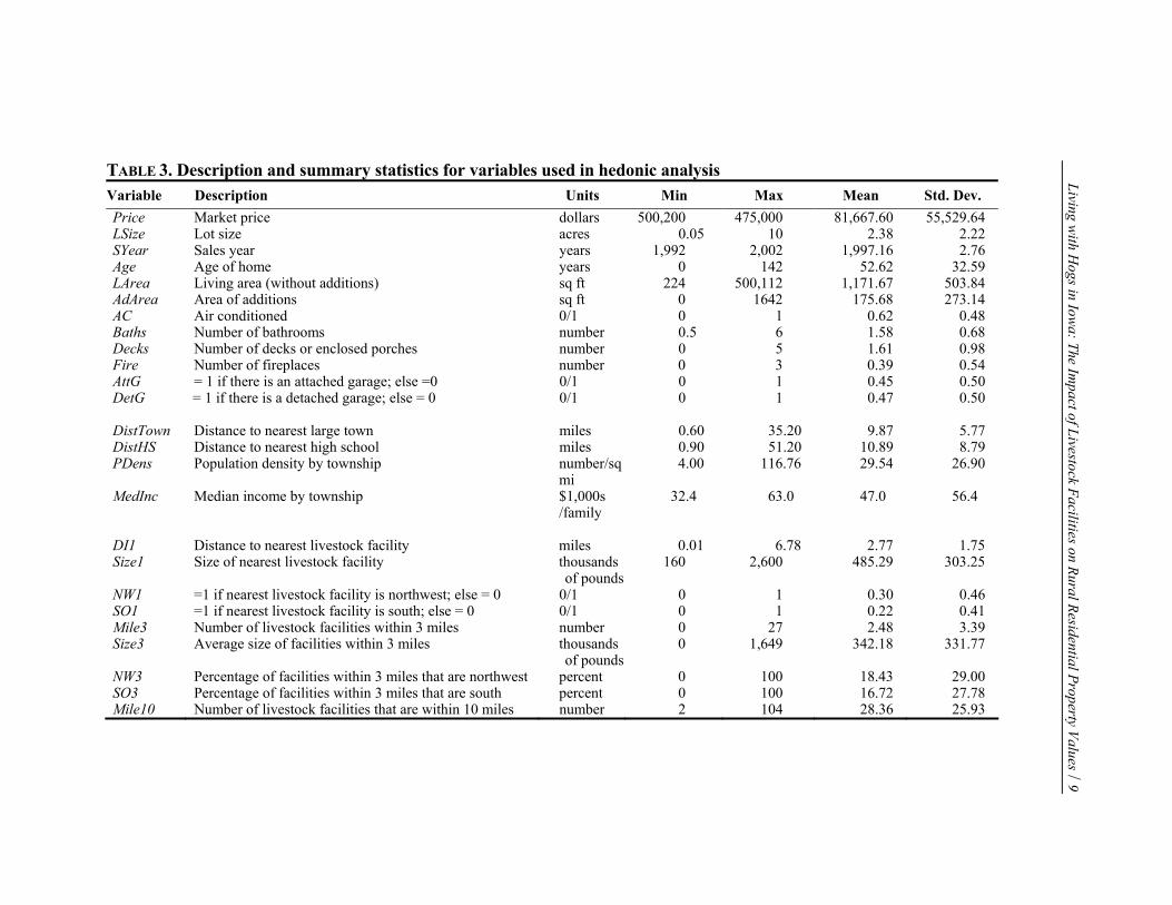
TABLE 3. Description and summary statistics for variables used in hedonic analysis Variable Description Units Min Max Mean Std. Dev. Price Market price dollars 500,200 475,000 81,667.60 55,529.64 LSize Lot size acres 0.05 10 2.38 2.22 SYear Sales year years 1,992 2,002 1,997.16 2.76 Age Age of home years 0 142 52.62 32.59 LArea Living area (without additions) sq ft 224 500,112 1,171.67 503.84 AdArea Area of additions sq ft 0 1642 175.68 273.14 AC Air conditioned 0/1 0 1 0.62 0.48 Baths Number of bathrooms number 0.5 6 1.58 0.68 Decks Number of decks or enclosed porches number 0 5 1.61 0.98 Fire Number of fireplaces number 0 3 0.39 0.54 AttG = 1 if there is an attached garage; else =0 0/1 0 1 0.45 0.50 DetG = 1 if there is a detached garage; else = 0 0/1 0 1 0.47 0.50 DistTown Distance to nearest large town miles 0.60 35.20 9.87 5.77 DistHS Distance to nearest high school miles 0.90 51.20 10.89 8.79 PDens Population density by township number/sq

mi 4.00 116.76 29.54 26.90

MedInc Median income by township $1,000s /family

32.4 63.0 47.0 56.4

DI1 Distance to nearest livestock facility miles 0.01 6.78 2.77 1.75 Size1 Size of nearest livestock facility thousands

of pounds160 2,600 485.29 303.25

NW1 =1 if nearest livestock facility is northwest; else = 0 0/1 0 1 0.30 0.46 SO1 =1 if nearest livestock facility is south; else = 0 0/1 0 1 0.22 0.41 Mile3 Number of livestock facilities within 3 miles number 0 27 2.48 3.39 Size3 Average size of facilities within 3 miles thousands

of pounds0 1,649 342.18 331.77

NW3 Percentage of facilities within 3 miles that are northwest percent 0 100 18.43 29.00 SO3 Percentage of facilities within 3 miles that are south percent 0 100 16.72 27.78 Mile10 Number of livestock facilities that are within 10 miles number 2 104 28.36 25.93

Living with H

ogs in Iowa: The Im

pact of Livestock Facilities on Rural Residential Property Values / 9


FIGURE 2. Residential sales locations

study site, we wanted to control for the possibility that a property could be affected by

more than one facility. Three groups of livestock facilities were identified for each

residential sales property: (a) the closest operation, (b) operations within 3 miles of the

property, and (c) operations within 10 miles of the property. The dataset contains 47

property sales that have at least one confinement located at ½ mile or less, 149 properties

with a confinement between ½ and 1 mile, and 491 properties with a confinement

between 1 and 3 miles.17 For the closest livestock operation, we calculated the distance to

the property (Dist1), the size of the nearest livestock facility (Size1), and whether the

facility was upwind of the property during the winter (NW1) or summer (SO1) seasons.18

As Table 3 indicates, the average distance to the nearest livestock facility is 2.8 miles and

ranges from just 0.01 to 6.8 miles. Roughly 30 percent of the nearest livestock facilities

are upwind of the sales sites during the winter months and 22 percent are upwind during

the summer months.


While the nearest livestock facility is likely to have the most direct impact on the

residential property value, the concentration of facilities in the region also may have an

impact. In addition to computing the total number of facilities within a 3-mile radius of

each property (Mile3), we also computed the average size of these facilities (Size3) and

the percentage that are upwind during the winter (NW3) and summer (SO3) seasons. As

Table 3 indicates, there is considerable variation in the concentration of facilities around

the residential sales site. While on average there are 2.5 livestock facilities within 3 miles

of the properties sold, this number ranges from 0 to 27 in the data set.19

Finally, we calculated the number of confinements in a 10-mile radius of each

property centroid. We hypothesized that the presence of a large number of confinements

within such a large radius might have a positive impact on local economic activity, while

the distance from the residential properties would be too large for odor to affect sale

values. As Table 3 indicates, the number of livestock confinements in the 10-mile radius

averages 28.4 and ranges from 2 to 104.

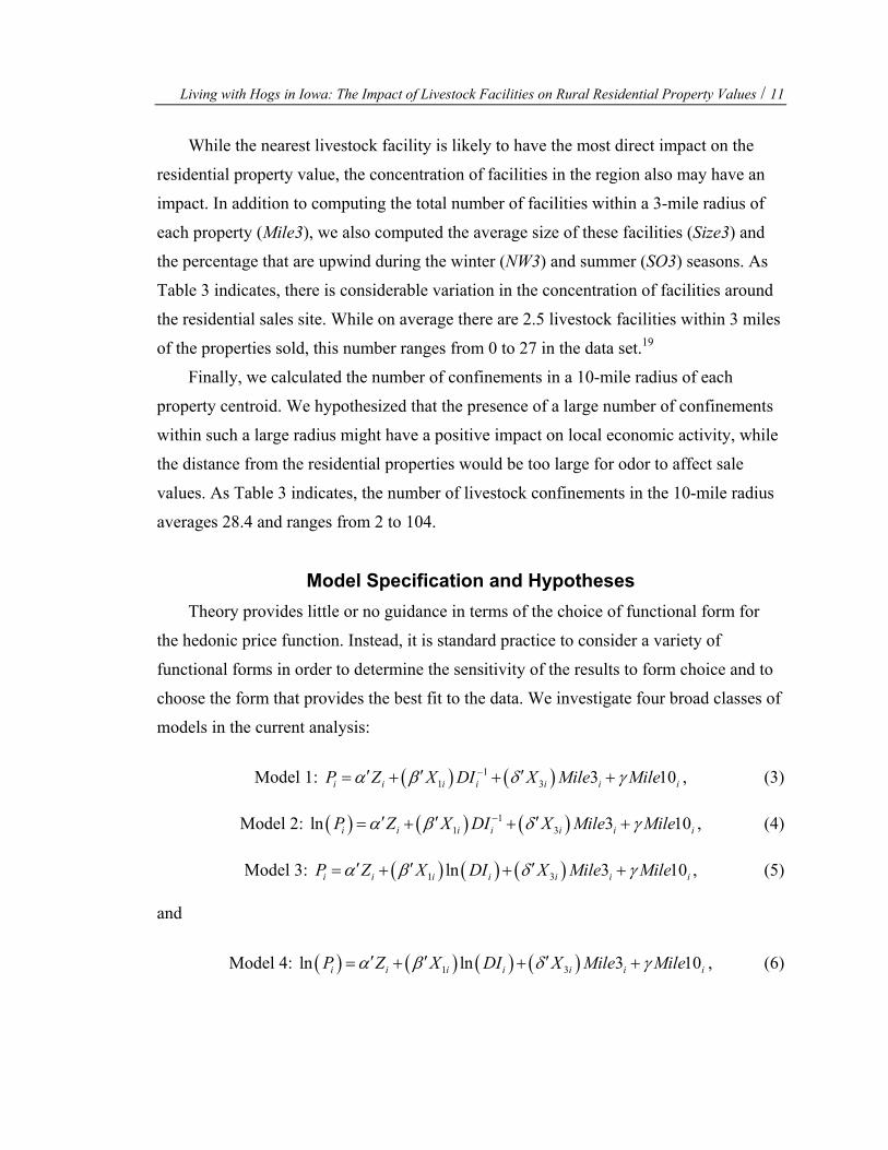
Model Specification and Hypotheses Theory provides little or no guidance in terms of the choice of functional form for

the hedonic price function. Instead, it is standard practice to consider a variety of

functional forms in order to determine the sensitivity of the results to form choice and to

choose the form that provides the best fit to the data. We investigate four broad classes of

models in the current analysis:

Model 1: ( ) ( )11 3 3 10i i i i i i iP Z X DI X Mile Mileα β δ γ−′ ′ ′= + + + , (3)

Model 2: ( ) ( ) ( )11 3ln 3 10i i i i i i iP Z X DI X Mile Mileα β δ γ−′ ′ ′= + + + , (4)

Model 3: ( ) ( ) ( )1 3ln 3 10i i i i i i iP Z X DI X Mile Mileα β δ γ′ ′ ′= + + + , (5)

and

Model 4: ( ) ( ) ( ) ( )1 3ln ln 3 10i i i i i i iP Z X DI X Mile Mileα β δ γ′ ′ ′= + + + , (6)


where iZ denotes the vector of structural and location characteristics for each sales unit

(i.e., the first two sets of variables in Table 3), 1iX denotes the vector of characteristics of

the nearest livestock facility for each home (i.e., size and wind direction dummies), and

3iX denotes the vector of characteristics of the facilities within 3 miles of each home. The

differences among the four groups of models lie in the forms of the dependent variable

and the distance to the nearest livestock facility. Models 1 and 3 have the sales price enter

linearly, whereas Models 2 and 4 use log-price as the dependent variable. In Models 1 and

2, the inverse distance to the nearest livestock facility is used, whereas in Models 3 and 4,

the distance to the nearest livestock facility enters in logarithmic form.20 In general, the

results of the hedonic regression analysis were similar across these four classes of models.

However, Model 4 (the double-log specification) provided the best fit.21

In addition to the basic model variations in equations (3) through (6), two alternative

measures of size were used for each livestock facility: live weight (pounds) and manure

production (pounds per year). Again, the qualitative finding reported as follows did not

change with the choice of these size measures. However, the models that include the live

weight measure dominated those based on manure production. In the results section, we

report only the results based on live weight measure. Thus, using the notation for the

variables listed in Table 3, the final model becomes

( )

( ) ( )

0

0

0

ln

ln 1 1 1 ln

ii Z i YR AG i LA i Ad i

AC i Bt i Dk i Fr i AG i DG i

Tw i HS i PD i MI i

i i iZ N S i

Price LSize SYear Age LArea AdArea

AirC Baths Decks Fire AttG DetG

DistTown DistHS PDens MedInc

Size NW SO DI

α α α α α α

α α α α α α

α α α α

β β β β

δ

= + + + + +

+ + + + + +

+ + + +

+ + + +

+ ( )ln 3 3 3 3

10

i i iZ N S i

i

Size NW SO Mile

Mile

δ δ δ

γ

+ + +

+

(7)

where the tildes above each variable indicate that they are measured relative to the mean

in the sample.22

There are a number of hypotheses of interest in terms of the hedonic price function.

Specifically, we consider the following four hypotheses:


• 0 : 0AH β δ γ= = = . This hypothesis corresponds to a test as to whether the

livestock facilities have any effect on rural residential property values.

• 0 : 0BH δ = . This hypothesis corresponds to a test as to whether concentration of

livestock facilities in the region has any effect on rural residential property values,

over and above the impact of the nearest facility.

• 0 : 0CH δ γ= = . This hypothesis corresponds to a test as to whether only the

nearest livestock facility affects a property.

• 0 : 0 0Dk kH kβ δ= = ∀ ≠ . This hypothesis corresponds to a test as to whether the

characteristics of the livestock facilities (i.e., size and wind direction) have any

effect on rural residential property values.

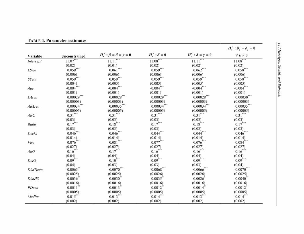
Results Table 4 provides the results of estimating the hedonic price equation in (7).

Coefficient estimates are presented for the unconstrained model and under each of the

hypotheses outlined in the previous section.

All of the structural characteristics of the home have the expected signs and are

statistically different from 0 at the 1 percent level or better. For example, each year of age

of the home reduces its value by roughly 0.4 percent, while a deck increases the home

value by 5 percent, and each fireplace increases the value by 8 percent. Moreover, the

coefficients change little across the various model specifications. Likewise, the location

variables, with the exception of distance to high school, have the expected size and signs.

Each mile away from the nearest large town diminishes the property value by

approximately 0.7 percent, whereas homes in areas with greater population densities

and/or higher median income levels are generally more valuable. The only unusual result

among the non-livestock factors is the coefficient on the distance to the nearest high

school. In general, one would expect that this coefficient would be negative, indicating

that easy access to the education system would increase the value of a home. However,

under all the model specifications considered, the coefficient on DistHS is positive and

significant at a 5 percent level or higher.

14 / H

erriges, Secchi, and Babcock

TABLE 4. Parameter estimates

Variable Unconstrained 0 : 0AH β δ γ= = = 0 : 0BH δ = 0 : 0CH δ γ= = 0 : 0

0

D

k kH

k

β δ= =

∀ ≠

Intercept 11.07*** (0.02)

11.11*** (0.01)

11.08*** (0.02)

11.11*** (0.02)

11.08*** (0.02)

LSize 0.059*** (0.006)

0.061*** (0.006)

0.059*** (0.006)

0.062*** (0.006)

0.058*** (0.006)

SYear 0.059*** (0.004)

0.059*** (0.005)

0.059*** (0.005)

0.059*** (0.005)

0.058*** (0.005)

Age -0.004*** (0.001)

-0.004*** (0.001)

-0.004*** (0.001)

-0.004*** (0.001)

-0.004*** (0.001)

LArea 0.00029*** (0.00003)

0.00028*** (0.00003)

0.00029*** (0.00003)

0.00028*** (0.00003)

0.00030*** (0.00003)

AdArea 0.00034*** (0.00005)

0.00035*** (0.00005)

0.00034*** (0.00005)

0.00034*** (0.00005)

0.00035*** (0.00005)

AirC 0.31***

(0.03) 0.31***

(0.03) 0.31***

(0.03) 0.31***

(0.03) 0.31***

(0.03) Baths 0.17***

(0.03) 0.18***

(0.03) 0.17***

(0.03) 0.18***

(0.03) 0.17***

(0.03) Decks 0.046***

(0.014) 0.046***

(0.014) 0.044***

(0.014) 0.044***

(0.014) 0.046***

(0.014) Fire 0.076***

(0.027) 0.081***

(0.027) 0.077***

(0.027) 0.076***

(0.027) 0.084***

(0.027) AttG 0.16***

(0.04) 0.17***

(0.04) 0.16***

(0.04) 0.16***

(0.04) 0.16***

(0.04) DetG 0.09***

(0.04) 0.10***

(0.03) 0.09***

(0.03) 0.09***

(0.03) 0.09***

(0.04) DistTown -0.0065**

(0.0025) -0.0070*** (0.0025)

-0.0068*** (0.0026)

-0.0066*** (0.0026)

-0.0070*** (0.0025)

DistHS 0.0036** (0.0016)

0.0030** (0.0016)

0.0035** (0.0016)

0.0026* (0.0016)

0.0040** (0.0016)

PDens 0.0011** (0.0005)

0.0013** (0.0005)

0.0012** (0.0005)

0.0014*** (0.0005)

0.0012** (0.0005)

MedInc 0.015*** (0.002)

0.013*** (0.002)

0.014*** (0.002)

0.013*** (0.002)

0.014*** (0.002)

Living with H

ogs in Iowa: The Im

pact of Livestock Facilities on Rural Residential Property Values/ 15

TABLE 4. Continued

*Statistically different from zero at a 10% level. **Statistically different from zero at a 5% level. ***Statistically different from zero at a 1%level.

Variable Unconstrained 0 : 0AH β δ γ= = = 0 : 0BH δ = 0 : 0CH δ γ= = 0 : 0

0

D

k kH

k

β δ= =

∀ ≠

LN(DI1) -0.009 (0.029)

-0.011 (0.026)

-0.038* (0.021)

0.029 (0.025)

Size1*LN(DI1) -0.064 (0.042)

-0.086** (0.040)

-0.075* (0.040)

NW1*LN(DI1) 0.052*

(0.029) 0.045

(0.029) 0.047

(0.029) SO1*LN(DI1) 0.036

(0.029) 0.031

(0.029) 0.033

(0.029) Mile3 0.0010

(0.0079) 0.0080

(0.0066) Size3*Mile3 -0.0060

(0.0169) NW3*Mile3 0.00043*

(0.00025) SO3*Mile3 0.00027

(0.00022) Mile10 0.0015

(0.0009) 0.0018**

(0.0008) 0.0011

(0.0009) LogLik -638.9 -649.2 -641.3 -644.3 -645.5 χ2 20.6*** 4.8 10.8* 13.2** Df 9 4 5 6 P-value 0.01 0.31 0.06 0.04


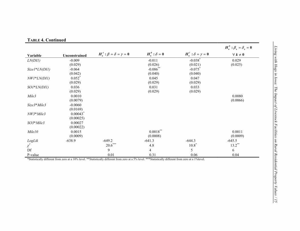
Turning to the livestock proximity factors, the unconstrained model in column 2 of

Table 4 indicates that few of these coefficients are individually significant. The

exceptions are the two wind direction variables associated with the winter season.

Specifically, the coefficient on the interaction term NW1*ln(DI1) is positive and

statistically significant at a 10 percent level. This indicates that for homes downwind of a

livestock facility during the winter season, an increase in the distance to the facility is

associated with a higher property value (i.e., proximity to the livestock facility is a

disamenity). While a similar point estimate applies to the summer wind direction

variable, it is not statistically significant. On the other hand, the coefficient on the

interaction term NW3*Mile3 is positive and significant at a 10 percent level, indicating

that a higher number of facilities in the region is generally associated with higher

property values. This may be capturing the positive impact of economic activity in the

region on property values.

While the livestock factors are not measured precisely on an individual basis, it is

apparent that they are significant as a group. In column 3 of Table 4, the hedonic price

coefficient estimates are presented under the hypothesis that all of the livestock factors

are 0. The associate likelihood ratio test statistic ( 29dfχ = =20.6) clearly rejects this

hypothesis with a p-value of 0.01. Livestock facilities apparently do have a significant

effect on rural residential property values in Iowa.

The lack of individual coefficient significance for the livestock variables may be due

in part to the high degree of correlation among some of the explanatory variables. In

particular, for many housing units the closest livestock facility is also the only livestock

facility within a 3-mile radius, resulting in substantial correlation among the ln(DI1) and

Mile3 variables. Column 4 of Table 4 considers a simpler specification for the livestock

variables, restricting the Mile3 factors all to 0. This hypothesis is not rejected at any

reasonable level. However, restricting both the Mile3 and Mile10 factors to be 0, as in

column 5, is clearly rejected. Finally, ignoring the size and wind direction characteristics

of the surrounding livestock facilities (as in the model presented in column 6) is also

rejected as a restriction.


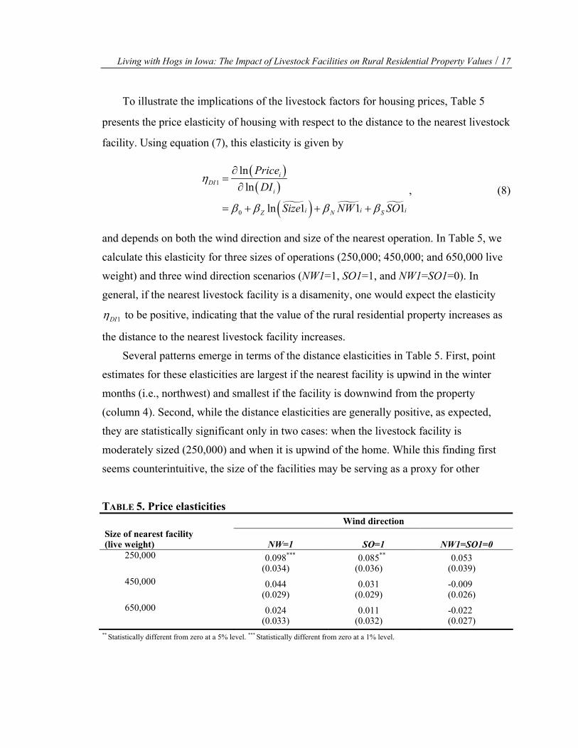
To illustrate the implications of the livestock factors for housing prices, Table 5

presents the price elasticity of housing with respect to the distance to the nearest livestock

facility. Using equation (7), this elasticity is given by

( )( )

( )1

0

lnln

ln 1 1 1

iDI

i

i i iZ N S

PriceDI

Size NW SO

η

β β β β

∂=

∂

= + + +

, (8)

and depends on both the wind direction and size of the nearest operation. In Table 5, we

calculate this elasticity for three sizes of operations (250,000; 450,000; and 650,000 live

weight) and three wind direction scenarios (NW1=1, SO1=1, and NW1=SO1=0). In

general, if the nearest livestock facility is a disamenity, one would expect the elasticity

1DIη to be positive, indicating that the value of the rural residential property increases as

the distance to the nearest livestock facility increases.

Several patterns emerge in terms of the distance elasticities in Table 5. First, point

estimates for these elasticities are largest if the nearest facility is upwind in the winter

months (i.e., northwest) and smallest if the facility is downwind from the property

(column 4). Second, while the distance elasticities are generally positive, as expected,

they are statistically significant only in two cases: when the livestock facility is

moderately sized (250,000) and when it is upwind of the home. While this finding first

seems counterintuitive, the size of the facilities may be serving as a proxy for other

TABLE 5. Price elasticities Wind direction

Size of nearest facility (live weight) NW=1 SO=1 NW1=SO1=0

250,000 0.098***

(0.034) 0.085**

(0.036) 0.053

(0.039) 450,000 0.044

(0.029) 0.031

(0.029) -0.009 (0.026)

650,000 0.024 (0.033)

0.011 (0.032)

-0.022 (0.027)

** Statistically different from zero at a 5% level. *** Statistically different from zero at a 1% level.


unobserved attributes of the confinement unit, including its age and the type of storage

system. In particular, most of the largest facilities in Iowa are relatively new and rely on

liquid manure storage systems. Additional research, including information on the

management and infrastructure of each livestock facility, is needed in order to

disentangle the dependence of the distance elasticity on facility size.

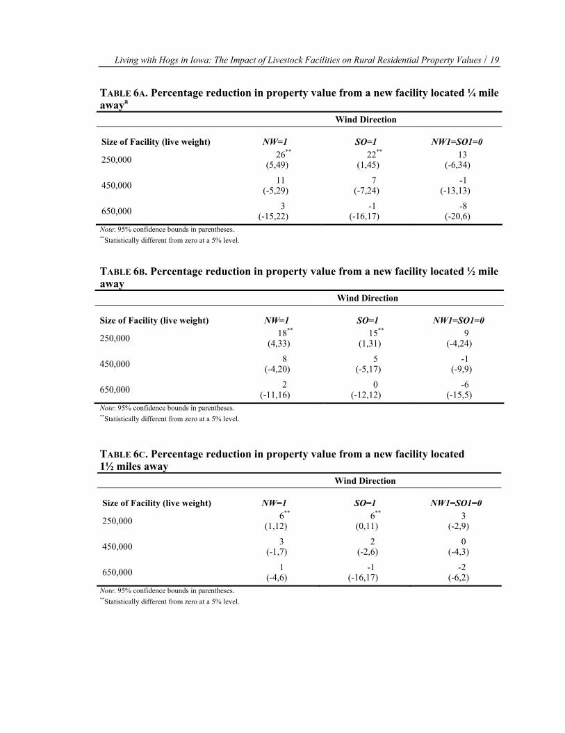
Finally, consider a rural residential property that currently has no livestock facility

located within a 3-mile radius. Tables 6a through 6c provide the predicted reductions in

property value that would result from a new livestock facility locating at various

distances away from a residence.23 For example, Table 6a considers locating the new

facility ¼ mile away from the home. The pattern of results, not surprisingly, is similar to

that found for the distance elasticities reported in Table 5. The impact is largest if the new

facility is located upwind of the home and is moderate in size (i.e., 250,000 pounds live

weight). Moreover, the property value reductions are statistically significant at a 95

percent confidence level only for the upwind and the moderate-sized facilities. In these

cases, the new facility would reduce the property value on average by 26 percent if

located northwest of the home and 22 percent if located south. For the average-sized

facility of 450,000 live weight, the percentage reductions are substantially smaller (less

than one-half) and statistically insignificant in all cases. Locating the new facility ½ mile

away from the residence (as in Table 6b) reduces the impact by 30 to 40 percent, but the

pattern remains the same in terms of statistical significance and the influence of wind

direction and size. Finally, locating the facility 1½ miles from the property (Table 6c)

further reduces the impact, with the property value reduction now ranging from roughly 0

to 6 percent.

Conclusions Iowa is an ideal place to raise livestock. The state has relatively few people,

abundant land, its crop sector imports fertilizer, and it has the lowest-cost feed. Yet,

currently it is quite difficult to build a new livestock feeding operation in Iowa because of

the opposition of rural residents. The estimated effects of proximity to livestock feeding

operations on property values in this study help explain the stalemate in siting new


TABLE 6A. Percentage reduction in property value from a new facility located ¼ mile awaya

Wind Direction

Size of Facility (live weight) NW=1 SO=1 NW1=SO1=0

250,000 26**

(5,49) 22**

(1,45) 13

(-6,34)

450,000 11 (-5,29)

7 (-7,24)

-1 (-13,13)

650,000 3 (-15,22)

-1 (-16,17)

-8 (-20,6)

Note: 95% confidence bounds in parentheses. **Statistically different from zero at a 5% level. TABLE 6B. Percentage reduction in property value from a new facility located ½ mile away

Wind Direction


250,000 18**

(4,33) 15**

(1,31) 9

(-4,24)

450,000 8 (-4,20)

5 (-5,17)

-1 (-9,9)

650,000 2 (-11,16)

0 (-12,12)

-6 (-15,5)

Note: 95% confidence bounds in parentheses. **Statistically different from zero at a 5% level. TABLE 6C. Percentage reduction in property value from a new facility located 1½ miles away

Wind Direction


250,000 6**

(1,12) 6**

(0,11) 3

(-2,9)

450,000 3 (-1,7)

2 (-2,6)

0 (-4,3)

650,000 1 (-4,6)

-1 (-16,17)

-2 (-6,2)

Note: 95% confidence bounds in parentheses. **Statistically different from zero at a 5% level.


operations in Iowa. The results suggest that there may be approximately a 10 percent

drop in property value if a new livestock feeding operation is located upwind and near a

residence. This drop in value helps explain opposition by rural residents to large-scale

feeding operations. Livestock supporters often admit there could be circumstances

whereby livestock facilities might affect property values, but they argue that the costs are

worth bearing because of the need to support a competitive industry in the state. From

their perspective, a 10 percent drop in the price of a $100,000 home is not large when

compared to investment costs of more than $300,000 for a new operation. The siting

stalemate reflects the political stalemate in Iowa. The state’s political leaders do not seem

to be able to resolve the problem because of the conflicting interests of important political

constituents.

This is a classic problem in which a production externality cannot be internalized

because of a lack of property rights. If rural residents were granted the right to be free of

damage, then our estimate of the magnitude of the effects of livestock facilities on

property values suggests room for mutually beneficial trading. If the willingness to pay to

site a feeding operation in Iowa exceeds the willingness to accept the damage caused by

the facility, then one would expect private negotiations to result in an agreement whereby

livestock operators would pay residents for the right to locate their feeding operations

nearby.

The results suggest that the magnitude of the payments that would have to be made

would be relatively modest if operators followed common sense siting rules. For

example, we cannot reject the hypothesis that siting a facility out of the path of prevailing

winds causes no damage. And the results are consistent with the expected finding that the

greater the distance between the facility and the residence, the less the damage. Thus, if

an operator would negotiate with residents located within a mile or so of a proposed site,

the site were located no closer than ½ mile of a resident, and no residence was located

downwind of the site, then we would expect the required payments to obtain the

acquiescence of the residents to be relatively modest.

Of course, our point estimates are only our best prediction of the average damages.

Actual damages depend on unmodeled effects such as local topographic features, site-

specific management practices, the type of manure storage and land application


techniques used, and other factors. Agreements between livestock feeders and rural

residents would have to include good faith provisions in which operators followed

prescribed management practices that are shown to reduce damage and subsequently

residents agreed to allow the feeding facility to remain in operation.

More precise estimates of the effects of feeding operations on property values could

be obtained by gathering more data about the attributes of the operations. In particular,

our finding that proximity to moderate-sized operations (250,000 pounds live weight)

results in greater damage to property values than proximity to large operations likely is a

result of different management practices employed at smaller units. Greater knowledge of

the management practices used on the various-sized units would allow us to better

estimate the effects of size on damage.

Endnotes

1. As Palmquist, Roka, and Vukina (1997) note, similar trends toward industry concentration have emerged in North Carolina, the second largest pork producer in the nation. By 1993, 13 percent of the producers were responsible for 95 percent of the state’s total swine production (Hurt and Zering 1993).

2. For the text of the bill, see <http://www.legis.state.ia.us/GA/79GA/Legislation/SF/ 02200/SF02293/Current.html>.

3. The case, heard by a Sac County jury, was Blass et al. vs. Iowa Select Farms, Inc.

4. Construction permits were also required for confinement feeding operations that used earthen storage and had an animal weight capacity of 200,000 pounds or more (400,000 or more pounds for bovine).

5. Freeman (2003, chap. 11) and Palmquist (1991) provide more complete overviews of theory underlying hedonic pricing analysis.

6. Farber (1998) provides a summary of recent studies of the impact of LULUs on property values.

7. Specifically, the house variables were the square footage, the age of the house, the number of bedrooms and bathrooms, and the assessor’s estimate of the ratio of house value to property value.

8. Wright County was originally included in our study area but eventually was dropped because of problems in obtaining residential sales data for the county.

9. Specifically, among the counties with a high density of livestock operations, Franklin has over 36 percent of moderate-sized facilities, Hamilton has 22 percent, and Hardin has 29 percent.

10. In order to properly account for proximity to animal operations for rural residential properties that were close to the county boundaries, we added a 10-mile buffer around the study area and included livestock facilities found in the buffer. The averages in Table 1 include facilities in the five-county study area (349) and the buffer zone (201).

11. There are two limitations to the livestock facilities data available for our analysis. First, we have information on only those operations in the five-county study area that are sufficiently large to require a manure management plan and/or a construc-


tion permit. Thus, we are not able to control for the impact of smaller livestock operations on rural residential property values. However, we were able to obtain data on all of the livestock facilities for Franklin County. This additional informa-tion did not change qualitatively the regression results for Franklin County. Second, the IDNR data does not provide a time series on the size (i.e., live weight) of each of the livestock facilities. Instead, we assumed that the operation size and locations were those reported in the manure management plan or construction permit filing and were constant over the study period. This creates a potential measurement error problem, particularly for those housing sales during the early 1990s. However, sensitivity analysis, excluding homes sold prior to 1996, again did not change the nature of the results.

12. The largest operation in the data set corresponds to an egg laying operation.

13. Because each assessor’s office had different filing systems, in some counties we were unable to obtain data for sales in the early 1990s.

14. DOQQs are available at <http://cairo.gis.iastate.edu/doqqs.html>.

15. Specifically, we used Sidwell’s online maps (<http://www.sidwellmaps.com/>) for Franklin and Humboldt counties, and copies of the assessor’s paper maps for Hamilton County. All data were analyzed in UTM Zone 15, NAD83.

16. We chose the 2,500 population cutoff in consultation with Daniel Otto, an Iowa State University Extension expert in economic and rural development. Towns over 2,500 were deemed large enough to serve as a hub of local economic activity, both in terms of employment and shopping.

17. It is worth noting that, according to Iowa law, operations built after January 1, 1999, have to comply with regulations on minimum distance to buildings and public use areas that range from 750 to 1,875 feet. Details about the regulation are available at the web site of the Iowa Department of Natural Resources, Water Quality Bureau.

18. The latter two wind direction variables were based on prevailing wind directions in Iowa (Mukhtar and Zhang 1995). Specifically, SO1=1 if the angle between the closest confinement and the house was between 135° and 255°, and NW1 = 1 if the angle between the closest confinement and the house was between 270° and 360°.

19. There are 458 properties that have no confinements within a 3-mile radius and 524 that have one to five operations within it. The remaining 163 properties have between 6 and 27 operations in the 3-mile radius.

20. Note that both the inverse distance and log distance ensure that the impact of a negative externality diminishes with distance.

21. The choice between the linear and logarithmic price specifications (i.e., Models 1 and 3 versus Models 2 and 4) was the most straightforward. Following PRV


(endnote 4), the sum of squared residuals from the two specifications were compared, after first normalizing observed prices by their geometric means. Palmquist and Danielson (1989) show that this is equivalent to using the Box-Cox criterion. The differences between using inverse distance and log-distances to the nearest site were less substantial, but the log-distance specification (i.e., Model 4) consistently dominated in terms of log-likelihood.

22. For example, i i iAge Age Age≡ − where iAge denotes the mean house age in the sample.

23. For the purposes of this exercise, we use the simpler hedonic price specification in column 4 of Table 4.

References

Abeles-Allison, M., and J. Conner. 1990. “An Analysis of Local Benefits and Costs of Michigan Hog Operations Experiencing Environmental Conflicts.” Agricultural Economics Report No. 536. Department of Agricultural Economics, Michigan State University.

Farber, S. 1998. “Undesirable Facilities and Property Values: A Summary of Empirical Studies.” Ecological Economics 24: 1-14.

Freeman, A. 2003. The Measurement of Environmental and Resource Values. Washington, D.C.: Resources for the Future.

Mubarak, H., T.G. Johnson, and K.K. Miller. 1999. The Impacts of Animal Feeding Operations on Rural Land Values. Report R-99-02. College of Agriculture, Food and Natural Resources, Social Sciences Unit, University of Missouri-Columbia. May.

Hurt, C., and K. Zering. 1993. “Restructuring the Nation’s Pork Industry.” In NC State Economist. North Carolina Cooperative Extension Service.

Iowa Department of Natural Resources, Water Quality Bureau. Animal Feeding Operations. <http://www.state.ia.us/government/dnr/organiza/epd/wastewtr/ feedlot/feedlt.htm> (accessed June 6, 2003).

Kiel, K. 1995. “Measuring the Impact of the Discovery and Cleaning of Identified Hazardous Waste Sites on House Values.” Land Economics 71(4): 428-35.

Kiel, K., and K. McClain. 1995a. “House Prices during Siting Decision Stages: The Case of an Incinerator from Rumor through Operation.” Journal of Environmental Economics and Management 28(2): 241-55.

———. 1995b. “The Effect of an Incinerator Siting on Housing Appreciation Rates.” Journal of Urban Economics 37: 311-23.

Kohlhase, J. 1991. “The Impact of Toxic Waste Sites on Housing Values.” Journal of Urban Economics 30: 1-26.

Lorimor J., W. Powers, and A. Sutton. 2000. “Manure Characteristics.” Manure Management Systems series, MWPS-18, Section 1. MidWest Plan Service, Iowa State University.

McCluskey, J., and G. Rausser. 2001. “Estimation of Perceived Risk and Its Effect on Property Values.” Land Economics 77(1): 42-55.

Mukhtar, S., and R. Zhang. 1995. “Guidelines for Minimizing Odors in Swine Operations.” Iowa State University Extension Publication Pm-1605. Iowa State University.

Palmquist, R. 1991. “Hedonic Methods.” In Measuring the Demand for Environmental Quality. Edited by J. Braden and C. Kolstad. Amsterdam: North Holland.


Palmquist, R., and L. Danielson. 1989. “A Hedonic Study of the Effects of Erosion Control and Drainage on Farmland Values.” American Journal of Agricultural Economics 71(February): 55-62.

Palmquist, R., F. Roka, and T. Vukina. 1997. “Hog Operations, Environmental Effects, and Residential Property Values.” Land Economics 72(1): 114-24.

Ready, R., and C. Abdalla. 2003. “The Amenity and Disamenity Impacts of Agriculture: Estimates from a Hedonic Pricing Model in Southeastern Pennsylvania.” Presented at the annual meeting of the American Agricultural Economics Association, Montreal, Canada, July 2003.

Reichert, A., M. Small, and S. Mohanty. 1992. “The Impact of Landfills on Residential Property Values.” Journal of Real Estate Research 7(2): 297-314.

Rosen, S. 1974. “Hedonic Prices and Implicit Markets: Product Differential in Perfect Competition.” Journal of Political Economy 82(1): 34-55.

Smith, V.K., and W. Desvousges. 1986. “The Value of Avoiding a Lulu: Hazardous Waste Disposal Sites.” Review of Economics and Statistics 68(2): 293-99.

Smith, V.K., and J. Huang. 1995. “Can Markets Value Air Quality? A Meta-Analysis of Hedonic Property Value Models.” Journal of Political Economy 103(1): 209-27.

Taff, S.J., D.G. Tiffany, and S. Weisberg. 1996. “Measured Effects of Feedlots on Residential Property Values in Minnesota: A Report to the Legislature.” Staff Paper P96-12. Department of Applied Economics, University of Minnesota. June.

Thayer, M., H. Albers, and M. Rahmatian. 1992. “The Benefits of Reducing Exposure to Waste Disposal Sites: A Hedonic Housing Value Approach.” Journal of Real Estate Research 7(2): 265-82.

Documents

Living with Hogs in Iowa: The Impact of Livestock ... · Living with Hogs in Iowa: The Impact of Livestock Facilities on Rural Residential Property Values Joseph A. Herriges, Silvia