Lithoflex tutorial 13giugno - Welcome to LithoFLEX.org lithoflex tutorial introduction 2 free mapping software geosoft 3 data format 3 data description / dummy values 4 study area

1

LithoFLEX Tutorial

INTRODUCTION 2

FREE MAPPING SOFTWARE GEOSOFT 3

DATA FORMAT 3

DATA DESCRIPTION / DUMMY VALUES 4

STUDY AREA 5

A. GRAVITY FORWARD CALCULATION 8

a) GRAVITY EFFECT OF AN UNDULATING LAYER BOUNDARY (DISCONTINUITY) 8

b) GRAVITY EFFECT OF SEDIMENTS 10

c) GRAVITY INVERSION: CALCULATION OF AN UNDULATING LAYER BOUNDARY 15

B. ISOSTATIC CALCULATIONS 27 a) FORWARD FLEXURE 29

b)TE-INVERSION 34 c)ANALYSIS OF THE MINIMUM RADIUS OF CONVOLUTION IN RELATION TO TE 24

C. TOOL GRIDS 38

a) CONCEPT OF EQUIVALENT TOPOGRAPHY 38

b) MAKE SYNTHETIC TOPOGRAPHY 38

E. TABLES OF INPUT AND OUT PUT FILE FOR LITHOFLEX 1.5 42

REFERENCES 46

Tutorial release data: 6/28/2008 Written by Susann Wienecke, Patrizia Mariani, Jörg Ebbing and Carla Braitenberg. Please send comments or questions to [email protected]

2

INTRODUCTION The tutorial describes the components in LITHOFLEX and the basic concepts for the use of the software package. The software LITHOFLEX provides a set of utilities to study the isostatic state and rheologic properties of the lithosphere. In addition, it includes a set of utilities that allow forward and inverse calculation of the gravity field for different scenarios. The tutorial contains the following sub-items, which are recommended to read in the following order: A. Gravity forward calculation

• Gravity effect of an undulating layer boundary

• Gravity effect of sediments

B. Gravity inversion: Calculation of an undulating layer boundary

C. Isostatic calculations

a) Forward flexure

b) Flexural inversion

c) Analysis of the minimum radius of convolution in relation to Te

D. Tool grids

a) Concept of equivalent topography

b) Make synthetic topography

E. Tables of input and output file for LITHOFLEX

3

FREE MAPPING SOFTWARE GEOSOFT It is suggested to link LITHOFLEX with an external viewer. Therefore please read "Getting started" in the Help file (LITHOFLEX/HELP). Geosoft provides free mapping software, which can be used as external viewer in order to plot the output grids. For more information visit: http://www.geosoft.com/pinfo/oasismontaj/free/montajviewer.asp.

DATA FORMAT The input files that are used in the tutorial are collect in the Zipped file Examples.zip. Please copy Examples.zip to a working folder of your convenience (e.g. D:\LithoWork) and unzip the file maintaining its original structure. In the following, when you find the instruction to go to the Examples folder, remember to go the position you copied the Examples folder into (e.g. D:\LithoWork\Examples). The Examples.zip file contains three subfolders: flexure, gravity and load and 10 tutorial grids. The first eight refer to an area of the Barents Sea, the last two refer to an area of the South China Sea (SCS). The SCS grids are used for application of Te inversion, as the tectonic setting is more suitable (Braitenberg et al., 2006). The following the tutorial grids are given:

1) grav.grd observed gravity data 2) sed.grd thickness of sediments 3) topo.grd bathymetry and topography (1100000 m sidelength-

extended size) 4) bathy.grd bathymetry (topography<0 m; extract with 400000 m

sidelength of the 1100000 m topo extended size) 5) basesed.grd top of basement, under the bottom of sediment thickness 6) load.grd equitopography 7) contrast_density example of synthetic contrast density grid 8) Var_te.grd example of synthetic Te variation grid 9) loadbig_SCS.grd equivalent topography

10) root_SCS.grd Moho discontinuity

required units for each dimension input grid x y z grav in m in m gravity in mGal (=10

-5·m/s

2)

load in m in m “z” axis is positive upward (in m)

topography in m in m “z” axis is positive upward (in m) bathymetry in m in m depth neg. downwards in m

sediment thickness in m in m thickness (positive) in m moho discontinuity in m in m depth neg. downwards in m

basesed in m in m depth neg. downwards in m contrast_density in m in m density contrast (ρc-ρm) in Mg/m3

Var_te in m in m Te in km

Table 1- Format of input grids.

4

LITHOFLEX generates output grids in Cartesian coordinates (e.g. UTM projected coordinates) and with the z-dimension as defined below (see Tab. 2).

required units for each dimension Output grid

X y z Discontinuity in m in m depth neg. downwards in m Boundary of gravity in m in m gravity in mGal (=10

-5·m/s

2)

Residual gravity in m in m gravity in mGal (=10-5

·m/s2)

Gravity of sediment in m in m gravity in mGal (=10-5

·m/s2)

Load of sediment in m in m depth neg. downwards in kg/ m2 Equiv. topography in m in m depth neg. downwards in m Load in m in m in m Moho discontinuity in m in m depth neg. downwards in m Te in m in m elastic thickness in km Flexure in m in m depth neg. downwards in m

Table 2- Format of output grids.

DATA DESCRIPTION / DUMMY VALUES It is very important for correct use of the software to keep the following things in mind:

• LITHOFLEX requires Surfer ASCII as input grid format. In addition, grids in the graphic-exchange-format (.gxf) can be imported and exported. Grids are not allowed to contain dummy values. Each module can call the internal routine GridMan to check the grids and give the user the possibility to change dummy values (e.g. –99999) to a reasonable value. In general, the use of dummy values should be avoided and the grid carefully prepared before using LITHOFLEX. For further information please use the help button on the gridMan form.

• The depth is negative downward and it is in meter; the Te grid only is in kilometer.

The user must check that the computer adopts the following international options:

1) in the Control Panel click on hours on language and international options; 2) then click on change the format of numbers, date and time \ customize \

numbers; Controls:

1) the decimal separator must be the point (“.”), and

5

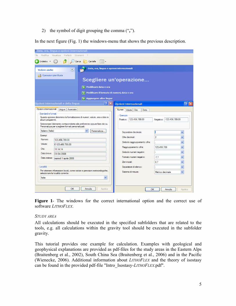
2) the symbol of digit grouping the comma (“,”). In the next figure (Fig. 1) the windows-menu that shows the previous description.

Figure 1- The windows for the correct international option and the correct use of software LITHOFLEX.

STUDY AREA All calculations should be executed in the specified subfolders that are related to the tools, e.g. all calculations within the gravity tool should be executed in the subfolder gravity. This tutorial provides one example for calculation. Examples with geological and geophysical explanations are provided as pdf-files for the study areas in the Eastern Alps (Braitenberg et al., 2002), South China Sea (Braitenberg et al., 2006) and in the Pacific (Wienecke, 2006). Additional information about LITHOFLEX and the theory of isostasy can be found in the provided pdf-file "Intro_Isostasy-LITHOFLEX.pdf".

6

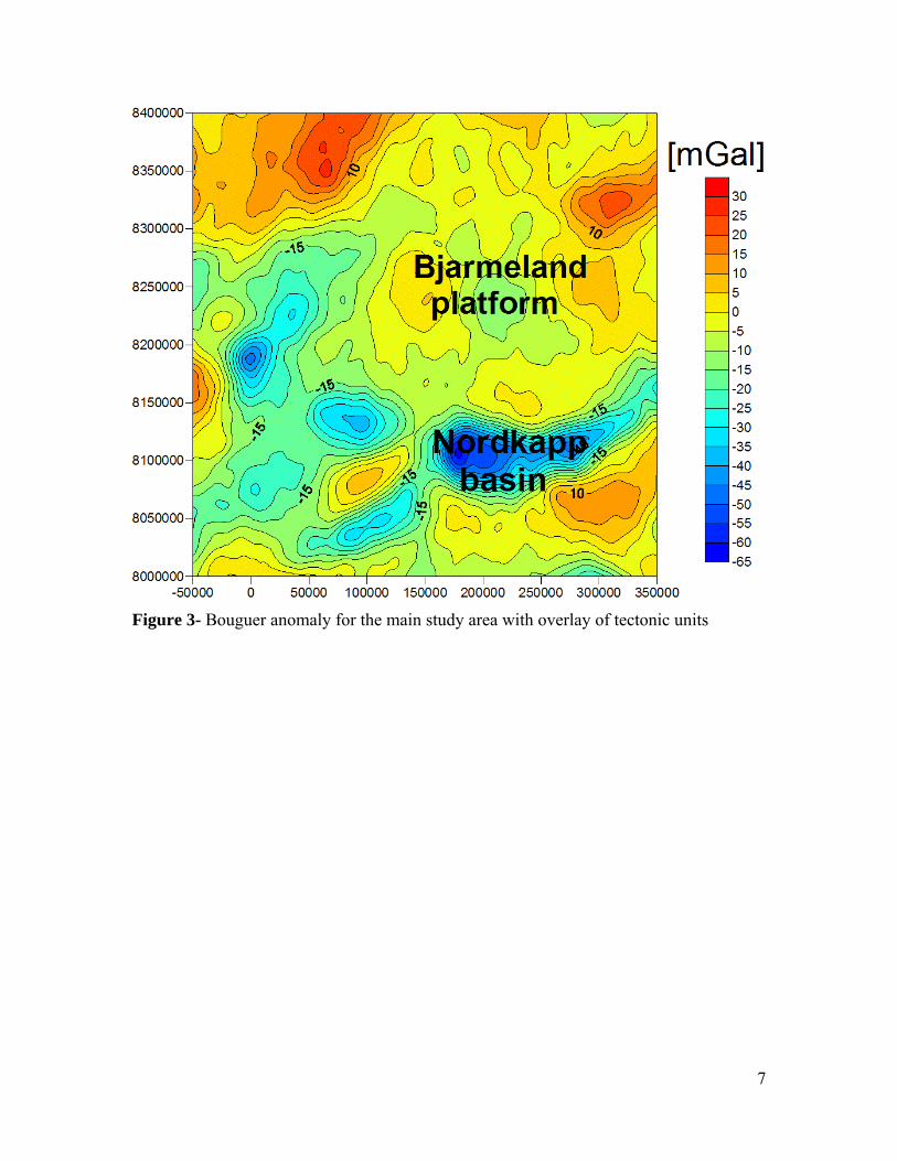
Figure 2- Topography of SW Barents Sea. Fig. 2 and Fig. 3 show the topography and the gravity for the tutorial study area of the SW Barents Sea. The most significant features are the Nordkapp basin in the southeast and the stable Bjarmeland platform in the central part.

7

Figure 3- Bouguer anomaly for the main study area with overlay of tectonic units

8

A. GRAVITY FORWARD CALCULATION

This chapter describes the forward calculation of the gravity effect for a predefined structure: a) for a layer dividing two bodies with a constant density contrast, or b) for sediment package with increasing density with depth.

a) GRAVITY EFFECT OF AN UNDULATING LAYER BOUNDARY (DISCONTINUITY) The gravity effect of an undulating discontinuity dividing two bodies with a constant density contrast is calculated by using the Parker algorithm (Parker, 1972), which makes use of series expansion up to order 5 of the gravity field generated by an oscillating boundary. The model can be applied e.g. for calculating the gravity field generated by the crust-mantle interface or for the gravity effect of the base of a sedimentary basin. As an example we create the base of the sediments, by subtracting the sediment thickness grid (sed.grd) from the topography grid (topo.grd) to calculate the base of the sediments. We use the tool GRIDS/Combine, to calculate the grid basesed.grd. After this step, the procedure is:

1. Copy the grid Examples/basesed.grd into the folder Examples/gravity/discontinuity/.

2. On the Gravity menu click Gravity Discontinuity.

3. Choose "basesed.grd" from the folder Examples/gravity/ discontinuity/ in the field for [Discontinuity]

4. Define the [Reference depth], e.g. "-5000" m, which defines the reference depth of the discontinuity.

5. Define the [Density Contrast], e.g. "-0.3", at the discontinuity between the upper and lower layer divided by the discontinuity. If "99" is given, a [Density grid] can be used. The use of a [Density grid] requires a pre-defined knowledge of the density distribution at the discontinuity, e.g. estimated from a seismic velocity model.

6. Give a name, e.g. "gravbasesed.grd" in the field [Gravity Field] for the calculated gravity effect of the discontinuity.

7. Click the [Execute] button. If the button turns blue, the calculation is finished.

The calculated file shows the gravity effect of the discontinuity (Fig. 4). One can now subtract this gravity effect from the observed gravity to reveal other sources. However, here we calculated only the gravity effect between a basin of constant infill density and the underlying basement. A more realistic calculation should consider sediment compaction with depth.

9

Figure 4- Gravity effect (gravbasesed.grd) of the discontinuity (base sediments).

10

B) GRAVITY EFFECT OF SEDIMENTS The gravity effect of sediments can be calculated by applying a function, which describes the change of densities in sediment package with depths. This is useful to reduce gravity data for the gravity effect of sediments, in order to investigate to resolve deep crustal structures (e.g. Moho, crustal intrusive). The function requires information about sediments thickness and the bathymetry as input data. Convention: here give depth parameters as negative values. First we prepare our input data:

1. Copy the grids Examples/bathy.grd and Examples/sed.grd into the folder Examples/gravity/sediments/.

2. On the Gravity menu click Gravity Forward Sediments. 3. Choose "sed.grd" from the folder Examples/gravity/sediments in the field for

[Sediment thickness], (see Fig. 5). 4. Choose "bathy.grd" from the folder Examples/gravity/sediments in the field for

[bathymetry/topography] 5. Give a cutoff period to filter the bathymetry and suppress short-wavelengths

features. E.g. write "20000" in the field for the [cutoff period] and all wavelengths smaller than 20 km will be suppressed in the calculations

6. Give a name, e.g. "batfilt.grd" for the output file of the low-pass filtered bathymetry. Click the [Filter] button to create the file in the folder Examples/gravity/sediments (see Fig. 6).

Next, a reference model for the calculations is defined. Gravity calculations are always done relative to a background density. In most applications a constant background can be used, but LITHOFLEX allows defining a two-layered reference model:

7. In the fields for [Density top, bottom] the densities, e.g. "2.67" and "2.85" at the top and at the bottom are defined. These values should correspond to a standard reference of two layers of continental crust.

8. In the field [depth top, bottom] the depth of the top and bottom, e.g. "0" and "-15000" m, of the upper layer of the reference model are defined. The depth range of the reference model should exceed the depth of the sedimentary basins. The top depth should in most applications be zero.

11

Figure 5- Thickness of sediments ranging from 1500 to 12000 m. AA’ indicates the location of a profile used later on for a discussion of parameter sensitivity.

Figure 6- Low pass filtered bathymetry. All wave lengths smaller than 20 km were removed.

In the next step we define the density-depth relation for the sediments:

12

9. The value in the field [Layer thickness] is used to divide the sediments in layers with the chosen thickness, e.g. "100" m, with changing density according to the defined depth-density relation. A small value gives higher precision, but requires longer computation time. A coarser value will approximate the sediment thickness poorly and can have the effect of discontinuities in the gravity field, if the sediment basin has steep flanks.

10. The density-depth relation can be defined on a linear or exponential scale. In the next step, we select first the linear variation and then the exponential function.

11. Linear compaction

Click [Linear variation]. The linear variation is defined by the parameters of upper and lower density of the linear density variation from [Top Density] to [Low Density] and the density below the linear variation [Bottom Density]. The linear variation is defined by the two depths [Top Depth] and [Low Depth]. [Top Depth] is in most applications "0" m, and [Low Depth] is given as negative value (e.g. "-12000" m). Define [Top Density], e.g. "2.25" Mg/m3 and [Top Depth], e.g. "0" m. Define [Low Density], e.g. "2.60" Mg/m3 and [Low Depth], e.g. "-12000" m. Define [Bottom density], e.g. "2.60" Mg/m3;

12. Give a name, e.g. "gsed_lin.grd" (instead of gsed.grd) in the field [Gravity of sediments] for the calculated gravity effect of the sediments.

13. Give a name e.g. "loadsed_lin.grd" (instead of loadsed.grd) in the field [Load of sediments] for the sedimentary loading, which can be further used for isostatic calculations.


The linear variation is calculated as follows: if the sediment-thickness is less than the absolute value of the depth [Low Depth], the density with depth rho(z) is: rho(z)=[Top Density]+([Low Density]-[Top Density]*(sedthickness)/([LowDepth]-

[LowDepth]) )/()()( toplowsedtoplowtop hhhz −−+= ρρρρ

otherwise:

rho(z)=[BottomDensity].

The gravity effect is then calculated by subtracting the density of the reference model from rho(z). In order to follow the calculated density with depth, an auxiliary file is created, named testsed_SI.dat. In the program the user can choose the coordinates of the density profile.

13

The file is structured as follows: rhoref1,rhoref2,dref1,dref2 (density reference model)

next columns are: #1 calculation depth z #2 depth of bathymetry #3 sediment thickness #4 reference density #5 density at depth z #6 density contrast at depth z (depends on the reference model) #7 effective load (Integrated sediment column from base sediments to

depth z) #8 sediment overburden

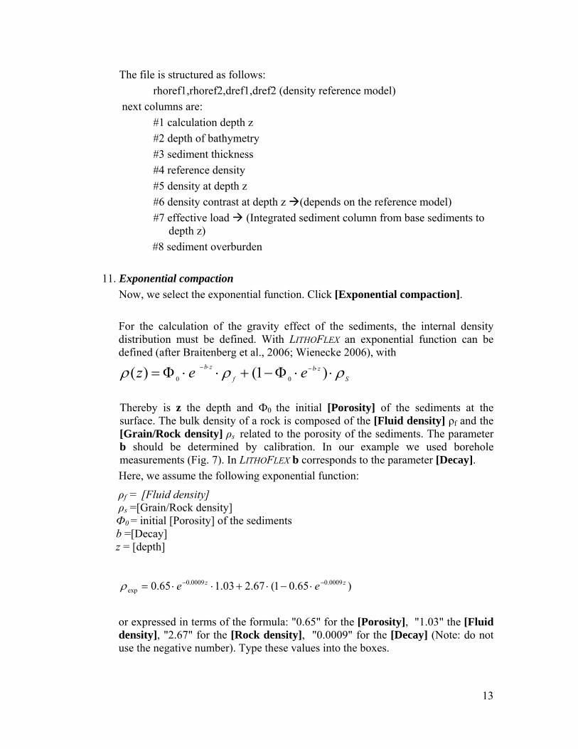
11. Exponential compaction

Now, we select the exponential function. Click [Exponential compaction]. For the calculation of the gravity effect of the sediments, the internal density distribution must be defined. With LITHOFLEX an exponential function can be defined (after Braitenberg et al., 2006; Wienecke 2006), with

Szb

f

zb eez ρρρ ⋅⋅Φ−+⋅⋅Φ= ⋅−⋅− )1()( 00

Thereby is z the depth and Ф0 the initial [Porosity] of the sediments at the surface. The bulk density of a rock is composed of the [Fluid density] ρf and the [Grain/Rock density] ρs related to the porosity of the sediments. The parameter b should be determined by calibration. In our example we used borehole measurements (Fig. 7). In LITHOFLEX b corresponds to the parameter [Decay]. Here, we assume the following exponential function:

ρf = [Fluid density] ρs =[Grain/Rock density] Ф0 = initial [Porosity] of the sediments b =[Decay] z = [depth]

)65.01(67.203.165.0 0009.00009.0exp

zz ee −− ⋅−⋅+⋅⋅=ρ

or expressed in terms of the formula: "0.65" for the [Porosity], "1.03" the [Fluid density], "2.67" for the [Rock density], "0.0009" for the [Decay] (Note: do not use the negative number). Type these values into the boxes.

14

Figure 7- Exponential density function to fit the borehole measurements in the Barents Sea. Tsikalas (1992) compiled all measured density values and used a linear relationship to describe the density increase with depth. Now, we can run our calculation:

12. Give a name, e.g. "gsed_expo.grd" (instead of gsed.grd) in the field [Gravity of sediments] for the calculated gravity effect of the sediments.

13. Give a name e.g. "loadsed_expo.grd" (instead of loadsed.grd) in the field [Load of sediments] for the sedimentary loading, which can be further used for isostatic calculations.


Figure 8- Gravity effect of the sediments using the exponential (Test 2) and the linear function.

15

15. The output files are now created in the same folder as the input files

Examples/gravity/sediments (see Fig. 8). Figure 8 shows the sedimentary gravity effect for the two alternative methods. Figure 9 shows the profile, along the maximum sediment thickness and close to the gravity minimum (see Fig. 5). Considering that this area is geologically complex, we provide also a synthetic example and its comparison with the exponential function and the linear function. To test the exponential compaction, we use different values for: exponential rock density, reference density, porosity and decay (see for the values see the Tab. 3).

Table 3- Tested values for the gravity effect of sediment.

In Figure 9 we show the effect of varying the matrix density (ρexp) of the sediments in the case of Test 1-4 listed in Tab. 3, along the profile AA’ shown in Fig. 9. In general a shift towards negative gravity values can be observed with decreasing matrix sediment density. With increasing density contrast (contrast density between the compaction density and the top layer of reference model) the gravity value increases, because the sediment density is greater than the top reference layer; the maximum gravity value corresponds to the maximum value of sediment thickness. When the density contrast is 0, the gravity anomaly is null. Applying a negative density contrast a minimum gravity signal is located over the maximum sediment thickness.

ReferenceModel

Exponential compaction

Linear Density

Ρ1 ρ2 Rock

density Decay Porosity

Top Low Bottom

Linear 2.67 2.85 2.25 2.60 2.60 Test 1 2.67 2.85 2.8 0.0009 0.65 Test 2 2.67 2.85 2.67 0.0009 0.65 Test 3 2.67 2.85 2.55 0.0009 0.65 Test 4 2.67 2.85 2.4 0.0009 0.65 Test 5 2.67 2.7 2.4 0.0009 0.65 Test 6 2.67 2.67 2.4 0.0009 0.65 Test 7 2.7 2.85 2.7 0.0009 0.65 Test 8 2.8 2.85 2.7 0.0009 0.65 Test 9 2.67 2.85 2.67 0.0009 0.45 Test 10 2.67 2.85 2.67 0.0009 0.75 Test 11 2.67 2.85 2.67 0.001 0.65 Test 12 2.67 2.85 2.67 0.0005 0.65

16

Figure 9- Gravity effect variation for varying exponential rock density. Tests 1-4 of density distribution (Tab. 3) along the profile AA’ (Fig. 5).

17

Figure 10- Variation of sediment gravity effect due to variation of top density, for the densities distribution cases 2-7-8 (Tab. 3) along the profile AA’ (Fig. 5). In Figure 10 we show the effect of variation of top density on the sediment gravity effect. Here we use a constant matrix density value (2.67) and we increase the top layer density (from 2.67 to 2.7 and 2.8). We observe the small difference between the Test 2 and 7, because the difference in the value for ρ1 is very small. In Figure 11 we give the gravity variation in relationship to the variation of bottom density. In this case the gravity value does not change, because the bottom of the sedimentary cover (where the maximum thickness is 12000 m), is above the top of the lower reference density (-15000 m).

18

Figure 11- Variation of sediment gravity effect for variation of bottom density, for the tests: 4, 5, 6, along the profile AA’ (Fig. 5).

19

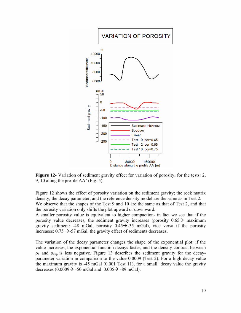
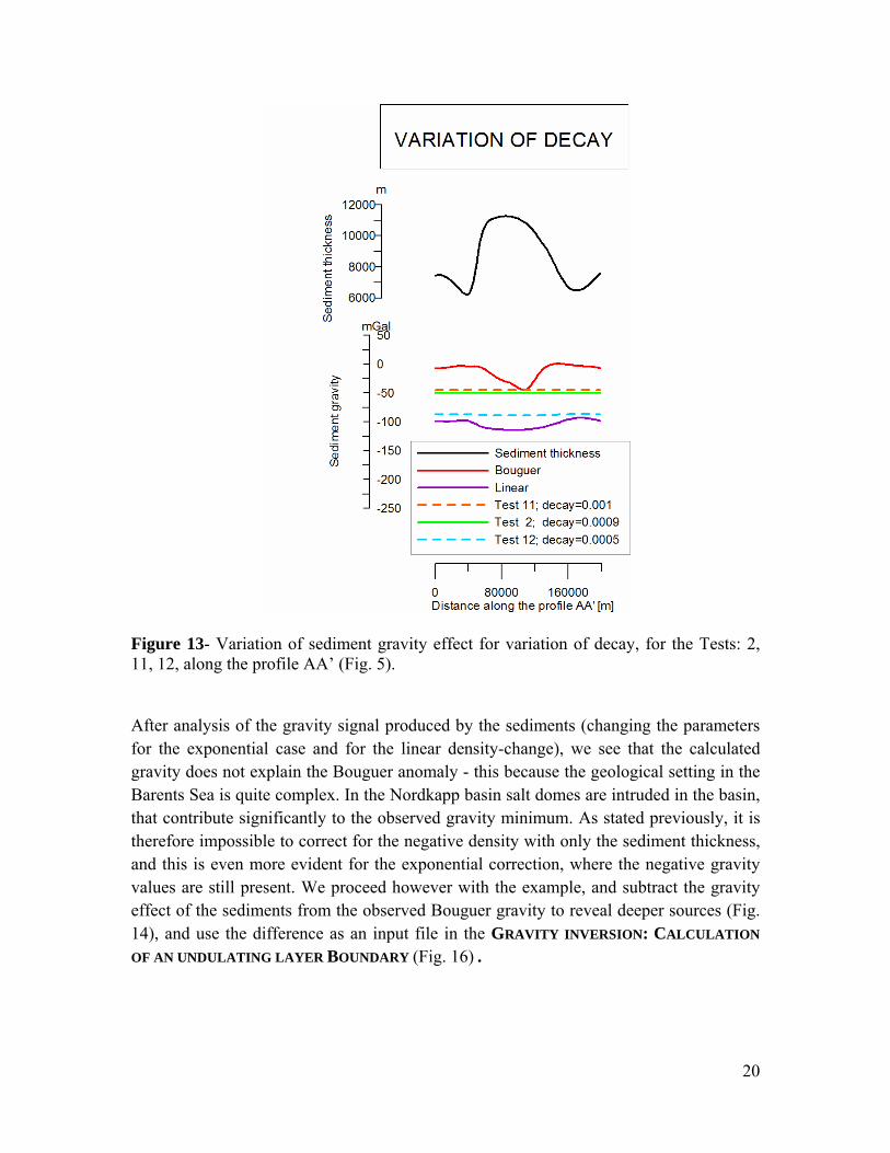
Figure 12- Variation of sediment gravity effect for variation of porosity, for the tests: 2, 9, 10 along the profile AA’ (Fig. 5). Figure 12 shows the effect of porosity variation on the sediment gravity; the rock matrix density, the decay parameter, and the reference density model are the same as in Test 2. We observe that the shapes of the Test 9 and 10 are the same as that of Test 2, and that the porosity variation only shifts the plot upward or downward. A smaller porosity value is equivalent to higher compaction- in fact we see that if the porosity value decreases, the sediment gravity increases (porosity 0.65 maximum gravity sediment: -48 mGal, porosity 0.45 -35 mGal), vice versa if the porosity increases: 0.75 -57 mGal, the gravity effect of sediments decreases. The variation of the decay parameter changes the shape of the exponential plot: if the value increases, the exponential function decays faster, and the density contrast between ρ1 and ρexp is less negative. Figure 13 describes the sediment gravity for the decay-parameter variation in comparison to the value 0.0009 (Test 2). For a high decay value the maximum gravity is -45 mGal (0.001 Test 11), for a small decay value the gravity decreases (0.0009 -50 mGal and 0.005 -89 mGal).

20

Figure 13- Variation of sediment gravity effect for variation of decay, for the Tests: 2, 11, 12, along the profile AA’ (Fig. 5). After analysis of the gravity signal produced by the sediments (changing the parameters for the exponential case and for the linear density-change), we see that the calculated gravity does not explain the Bouguer anomaly - this because the geological setting in the Barents Sea is quite complex. In the Nordkapp basin salt domes are intruded in the basin, that contribute significantly to the observed gravity minimum. As stated previously, it is therefore impossible to correct for the negative density with only the sediment thickness, and this is even more evident for the exponential correction, where the negative gravity values are still present. We proceed however with the example, and subtract the gravity effect of the sediments from the observed Bouguer gravity to reveal deeper sources (Fig. 14), and use the difference as an input file in the GRAVITY INVERSION: CALCULATION

OF AN UNDULATING LAYER BOUNDARY (Fig. 16) .

21

Figure 14- Sediment correction: Bouguer gravity minus Exponential (Test 2) and Linear sediment gravity. Testsed_Si.dat Here we describe the file Testsed_SI.dat, which is composed of 8 columns:

Column 1 calculation depth z Column 2 Depth of bathymetry Column 3 sediment thickness Column 4 reference density Column 5 density at depth z Column 6 density contrast at depth z (depends on reference model) Column 7 effective load Integrated sediment column from base sediment

to depth z Column 8 sediment overburden

Table 4- Description of Testsed_SI.dat.

Now we give a few plots (Fig. 15) to represent Testsed_SI.dat, as a function of column A, the depth. The plot represents the analysis of Forward flexure/Exponential case for the tests (Tab. 3), where the coordinates of the test-point are: Easting 150000 m, Northing 8200000 m. We show the comparison between: Linear density (test: Linear) and Exponential compaction (Test 2). In Fig. 15 a) the x-axis is the column 2, the depth of the bathymetry for the test-point. Here the bathymetry is about 334 m, but the sediment thickness is over 8600 m (Fig. 15 b, using the column 3 for the x-axis).

22

The next three plots show the density variation in function of depth. • the plot c) shows the reference density. In our case we only see the top density

layer (2.67 Mg/m3). • the plot d) shows the density variation in relationship to depth for the exponential

and linear models. • the plot e) shows the density contrast (ρexp - ρ1 e.g: 2.67-2.67=0) for the

exponential test and for the linear test (from 2.25 to 2.60). The density is equal to zero, when the depth is outside the range of the sediments. In our case the sediments start at -334 m, below the ocean bottom. The linear case shows a density increase up until to -9000 m. In Fig. 15 f) the integration of the sediment from the base sediment to depth z is shown, and in h) the sediment overburden at depth z is shown.

23

Figure 15- Plot of Testsed_SI.dat in function of depth, for every column, for the test Linear and exponential (Test 2); in “linear” we use: ρ1= 2.67; ρ2= 2.85;. ρtop=2.25, ρlow=2.60, ρbottom=2.60.

b) GRAVITY INVERSION: CALCULATION OF AN UNDULATING LAYER BOUNDARY

Here, we describe how to derive an undulating boundary or discontinuity (that often corresponds to the Moho) from observed gravity data by gravity inversion. Theoretically, small wavelength anomalies in the observed gravity field correspond to the sediments and intra crustal density inhomogeneities, while the long wavelength information corresponds to the crust/mantle density contrast. However, sedimentary basins can also produce a long wavelength signal. Therefore it is suggested to calculate the gravity effect of sediments in a first step (see chapter GRAVITY EFFECT OF SEDIMENTS): 1. Copy the grid Examples/grav.grd into the folder Examples/gravity/inversion. If the

gravity effect of sediments was calculated (e.g. the gravity effect of linear compaction), copy the grid Examples/gravity/sediments/gsed_lin.grd into the folder Examples/gravity/inversion.

2. If no gravity effect of the sediments should be taken into account, perform steps 9-18, otherwise continue with the next Step.

3. On the Grids menu, then click Combine Grids. 4. Choose "grav.grd" in the field for [Open grid 1] and "gsed_lin.grd" in the field for

[Open grid 2] from the folder Examples/gravity/inversion/ 5. Give a name, e.g. "combined.grd" for the [Output file]. 6. Click [Subtraction] as the "Grid operation" to subtract Grid 2 from Grid 1. 7. Click the [Execute] button. 8. The output file is now created in the same folder as the input files

24

Examples/gravity/inversion 9. On the Gravity menu click Gravity Inversion, if no gravity effect of the sediments

should be used, choose "grav.grd" from the folder Examples/gravity/inversion/ in the field for [InputGravity]. If the gravity effect of the sediments should be used, choose "combined.grd" from the folder Examples/gravity/inversion/ in the field for [InputGravity].

10. Define the [Reference depth], e.g. "-30000" m, which defines the normal, average depth of the discontinuity.

11. Define the [Density Contrast], e.g. -"0.35", at the discontinuity between the upper and lower layer divided by the discontinuity.

12. E.g. write “100000” in the field for the [Pmin minimum period] to define a cut-off wavelength for filtering the input gravity field that suppresses all wavelengths smaller than 100 km.

13. Define the number of iterations [No. iterations], e.g. "3". 14. Give a name, e.g. "root_final.grd" for the output file of calculated discontinuity in the

field [Output Surface]. 15. Give a name, e.g. "gravroot.grd", for gravity effect of the boundary in the field

[Boundary Gravity]. 16. Give a name, e.g. "gresid.grd ", for the difference between the input gravity and the

gravity effect of the boundary in the field [Residual Gravity]. 17. Click the [Execute] button. If the button turns blue, the calculation is finished 18. The output files are now created in the same folder as the input files

Examples/gravity/inversion (see Fig.16).

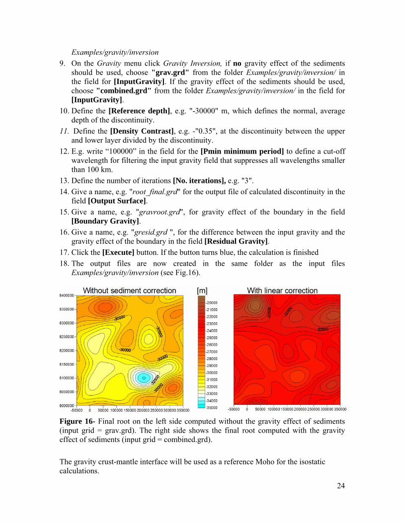
Figure 16- Final root on the left side computed without the gravity effect of sediments (input grid = grav.grd). The right side shows the final root computed with the gravity effect of sediments (input grid = combined.grd).

The gravity crust-mantle interface will be used as a reference Moho for the isostatic calculations.

25

In the Gravity Inversion, it can use a [density contrast] grid for input file. The simple example file is contrast_density.grd. In order to load this grid write 99 in the density value, and after that one can add the density input file. We select a synthetic profile along BB’ (see location in Fig. 17) to study the relevant quantities (Fig.18).

Figure 17- Density contrast (the second input file for Gravity Inversion) and BB’profile (see Fig.18).

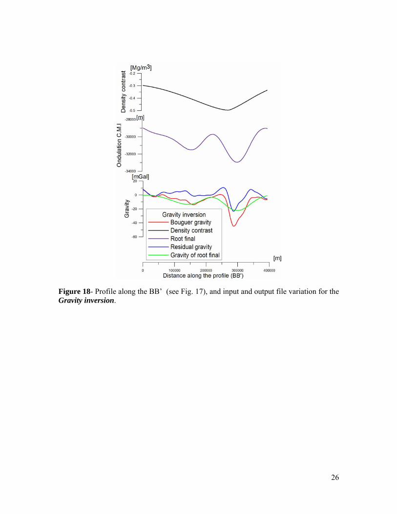
In Figure 18 the red and black lines show the input files: the Bouguer gravity and the density contrast. The other lines are: in violet the undulation of the Crust Mantle Interface (C.M.I), which is the output file named “final_root.grd”. The green line shows the calculated gravity of the final root (“gravroot.grd” is the output file), and the blue line gravity residual (difference between “observed” and modeled gravity (“gresid.grd” is the output file). In general an increased negative density contrast (-0.5 Mg/m3) decreases the oscillation- amplitude of the C.M.I.

26

Figure 18- Profile along the BB’ (see Fig. 17), and input and output file variation for the Gravity inversion.

27

ISOSTATIC CALCULATIONS In the concept of isostasy the topographic masses are floating on the mantle. The Airy

and Pratt model of isostasy assume that the topography is locally compensated. The

Vening-Meinesz Model describes a regional compensation, assuming that the

topographic masses are situated on a crustal plate, which is flexed due to loading (Fig.

19). The most important assumption of the Vening-Meinesz model is, that the lithosphere

behaves as a perfectly elastic material. The flexure of the plate depends on the

topographic load and internal loads (crustal inhomogeneities within the plate). However,

the most important factor that controls the bending of the plate is the flexural rigidity. If

the crustal plate has a high flexural rigidity, then almost no "root" is produced and the

deflection is small. For a low flexural rigidity the deflection is larger and a larger root

will be produced. If the flexural rigidity is zero, then the solution for the flexure of the

crustal plate converges to the Airy isostatic case.

The bending of the plate is described with a differential equation of 4th order, which is

solved with a Fast Fourier transformation within LITHOFLEX. The flexural compensation

surface (e.g. Moho) is estimated applying a thin plate approximation, where the solutions

for a low elastic thickness value (e.g. Te=1 km) converge to the Airy isostatic case

(Wienecke, 2006).

28

Figure 19- Different behaviour for the flexure of a plate depending on its flexural rigidity. The flexural rigidity D is expressed by the elastic thickness Te, the Young's modulus E and the Poisson's ratio ν with the equation:

Commonly standard values are used for the Young's modulus E=100GPa= 10

11N/m

2 and

the Poisson's ratio ν = 0.25 and the terms flexural rigidity and elastic thickness are used synonymously. LITHOFLEX allows both to calculate the flexural response surface for a given loading, and to invert for the flexural distribution of a given area.

29

a) FORWARD FLEXURE This chapter describes how to calculate the flexural surfaces for a given loading by topography and/or sediments. LITHOFLEX gives three possibilities, using: 1) the spectral method: on the Tool menu click: Flexure/Forward Flexure/Fixed elastic thickness/fast; 2) the convolution method: on the Tool menu click: Flexure/Forward Flexure/Fixed elastic thickness/precise. The convolution method uses the analytical flexure response functions of Wienecke (2006). 3) the convolution method applied with a grid of variable elastic thickness: on the Tool menu click: Flexure/Forward Flexure/Variable elastic thickness/precise. Also in this case the analytical flexure response functions of Wienecke (2006) are used. To estimate the flexure of the crust-mantle interface or Moho, it is important to take the loading by the water into account. This can be done by calculation of the equivalent topography (see tutorial HOW TO CREATE AN EQUIVALENT TOPOGRAPHY). In the following the spectral method is applied:

1. Copy the grid Examples/load.grd into the folder Examples/flexure/forward flexure/.

2. Go to the Flexure menu, and click [Forward Flexure/fast] for [Fixed Elastic Thickness].

3. Choose "load.grd" in the field for [Input Load] from the folder Examples/ flexure/forward flexure/.

4. Define the [Te Max], e.g. "15" km, which defines the maximum elastic thickness for which the flexural response is calculated.

5. Define the [Te Min], e.g. "5" km, which defines the minimum elastic thickness for which the flexural response is calculated.

6. Define the [Delta Te], e.g. "5" km, which defines the step size between [Te min] and [Te max] for which the flexural response is calculated.

In this example three flexure surfaces are calculated with Te=5 km, Te=10 km and Te=15 km.

7. Define the [Reference Depth], e.g. "-30000" m, which defines the normal, reference depth of the flexure surface. The reference depth defines the level of the flexure surface for null load.

30

8. Ignore the [Distance from margin], because in the spectral domain the program does not use this value.

9. Define the [Young's modulus], e.g. "1.0" 1011 N/ m2 used for the calculation.

10. Define the [Gravity], e.g. "9.81" m/s2, which is the absolute, normal gravity.

11. Define the [Poisson ratio], e.g. "0.25" used for the calculation.

12. Define the [Crust density], e.g. "2.7" Mg/m3 used for the calculation.

13. Define the [Mantle density], e.g. "3.2" Mg/m3 used for the calculation.

14. Give a name, e.g. "flexure.grd" for the output file of the calculated flexure response in the field [Output Grid].

15. Click the [Execute] button. If the button turns blue, the calculation is finished and three flexure surfaces are calculated in the subfolder Examples/flexure/forward flexure, named “flexure5.grd”, “flexure10.grd” and “flexure15.grd corresponding to Te=5 km, 10 km and 15 km, respectively. In Fig. 20 you see the flexure5.grd”, “flexure10.grd” and “flexure15.grd” for the spectral method.

Figure 20- Flexural crust-mantle interface for the spectral method, for Te= 5 km, 10 km, 15 km, we add the color scale of the convolution method (see Fig. 21) for comparison. The green rectangle shows an area that will be later on studied by applying the flexural convolution method. The figure shows also clearly border effects of the margins of the study area.

Next, we describe the convolution method:

31

1. Copy the grid Examples/load.grd into the folder Examples/flexure/forward flexure

2. Go the Flexure menu, and then click [Forward Flexure] and select which method to use for calculating the flexural response to the loading. Click "Precise" for [Fixed Elastic Thickness] 3. Choose "load.grd" in the field for [Input Load] from the folder Examples/ flexure/forward flexure.

4. Define the [Te Max], e.g. "15" km, which defines the maximum elastic thickness for which the flexural response is calculated.

5. Define the [Te Min], e.g. "5" km, which defines the minimum elastic thickness for which the flexural response is calculated.

6. Define the [Delta Te], e.g. "5" km, which defines the step size between [Te min] and [Te max] for which the flexural response is calculated.

In this example three flexure surfaces are be calculated with the analytical solution, for Te=5 km, Te=10 km and Te=15 km.

7. Define the [Reference Depth], e.g. "-30000" m, which defines the normal, average depth of the flexure surface.

8. Define the [Distance from margin], e.g. “350000” m, which reduces the calculation area respect to [Input Load] "load.grd" at each side in order to avoid edge effects.






14. Give a name, e.g. "flexure_precise.grd" (instead of flexure.grd) for the output file of the calculated flexure response in the field [Output Grid].

15. Click the [Execute] button. If the button turns blue, the calculation is finished and three flexure surfaces are calculated in the subfolder Examples/flexure/forward flexure, named “flexure_precise5.grd”, “flexure_precise10.grd” and “flexure_precise15.grd corresponding to Te=5 km, 10 km and 15 km, respectively (Fig. 21).

32

Figure 21- Flexural crust-mantle interface for the convolution method, for Te= 5, 10, 15 km.

Next, the convolution method with a grid of variable elastic thickness is applied:

1. Copy the grid Examples/load.grd and the grid Var_te.grd into the folder Examples/flexure/forward flexure/.

2. Go to the Flexure menu, and then click Forward Flexure and select "Precise" for [Variable Elastic Thickness], which requires a pre-defined grid of Te distribution over the study area.

3. Choose "load.grd" in the field for [Input Load] from the folder Examples/ flexure/forward flexure/.

4. Choose the second input file: [varTe.grd] from the folder Examples/ flexure/forward flexure/.

In this examples one flexure surface will be calculated with the analytical solution, and assuming a variable Te grid

8. Define the [Reference Depth], e.g. "-30000" m, which defines the normal, average depth of the flexure surface.

9. Define the [Distance from margin], e.g. “50000” m, which reduces the calculation area respect to [Input Load] "load.grd" at each side in order to avoid edge effects.




33



15. Give a name, e.g. "mo_varTe.grd" for the output file of the calculated flexure response in the field [Output Grid].

16. Click the [Execute] button. If the button turns blue, the calculation is finished .

Figure 22- Left: Te variation (example input grid); Right: resulting Moho depth for this Te variation.

34

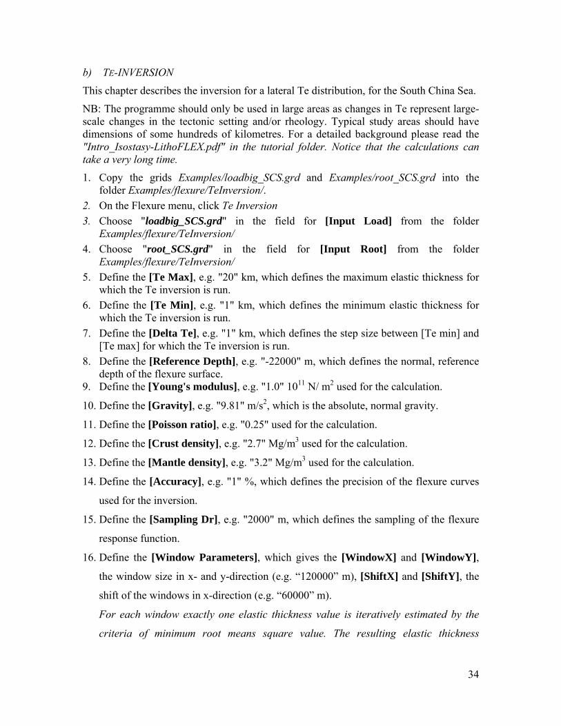
b) TE-INVERSION

This chapter describes the inversion for a lateral Te distribution, for the South China Sea.

NB: The programme should only be used in large areas as changes in Te represent large-scale changes in the tectonic setting and/or rheology. Typical study areas should have dimensions of some hundreds of kilometres. For a detailed background please read the "Intro_Isostasy-LithoFLEX.pdf" in the tutorial folder. Notice that the calculations can take a very long time.

1. Copy the grids Examples/loadbig_SCS.grd and Examples/root_SCS.grd into the folder Examples/flexure/TeInversion/.

2. On the Flexure menu, click Te Inversion 3. Choose "loadbig_SCS.grd" in the field for [Input Load] from the folder

Examples/flexure/TeInversion/ 4. Choose "root_SCS.grd" in the field for [Input Root] from the folder

Examples/flexure/TeInversion/ 5. Define the [Te Max], e.g. "20" km, which defines the maximum elastic thickness for

which the Te inversion is run. 6. Define the [Te Min], e.g. "1" km, which defines the minimum elastic thickness for

which the Te inversion is run. 7. Define the [Delta Te], e.g. "1" km, which defines the step size between [Te min] and

[Te max] for which the Te inversion is run. 8. Define the [Reference Depth], e.g. "-22000" m, which defines the normal, reference

depth of the flexure surface. 9. Define the [Young's modulus], e.g. "1.0" 1011 N/ m2 used for the calculation.





14. Define the [Accuracy], e.g. "1" %, which defines the precision of the flexure curves

used for the inversion.

15. Define the [Sampling Dr], e.g. "2000" m, which defines the sampling of the flexure

response function.

16. Define the [Window Parameters], which gives the [WindowX] and [WindowY],

the window size in x- and y-direction (e.g. “120000” m), [ShiftX] and [ShiftY], the

shift of the windows in x-direction (e.g. “60000” m).

For each window exactly one elastic thickness value is iteratively estimated by the

criteria of minimum root means square value. The resulting elastic thickness

35

distribution has a higher spatial resolution for a smaller window size. The value

should be chosen in consideration of the grid node distance of the input grids.

17. Define the [Distance from margin], e.g. “200000 m, which reduces the calculation

area respect to [Input Load] "load.grd" at each side in order to avoid edge effects. 18. Give a name, e.g. "te.grd" in the field [Output Te Grid] for the output file of the Te

distribution after running the inversion 19. Give a name, e.g. "mo.grd" in the field [Output Flexure Moho] for the flexural

response related to the final Te distribution after running the inversion 20. Give a name, e.g. "mor.grd" in the field [Output Residual (Root- Flexure) Moho]

for the difference between the input root and the best-fit flexural response surface related to the final Te distribution after running the inversion

21. Give a name, e.g. "admicur" in the field [Administration File] to log all parameters used for the inversion


Input file : 1)loadbig_SCS.grd 2)Root_SCS.grd (built by Gravity inversion)

Figure 23- The input for Te inversion, South China Sea. Left: equivalent topography (grid “Loadbig_SCS.grd”), right: crust mantle boundary from gravity inversion.

In this inversion the sediments in the study area are not taken in account (Fig. 24).

36

Figure 24- Output files for the South China Sea example: a) isostatic Moho depth, b) Te variation, c) residual Moho: difference between input and output Moho.

37

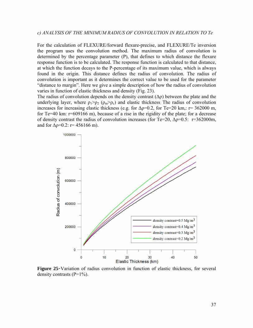
c) ANALYSIS OF THE MINIMUM RADIUS OF CONVOLUTION IN RELATION TO Te For the calculation of FLEXURE/forward flexure-precise, and FLEXURE/Te inversion the program uses the convolution method. The maximum radius of convolution is determined by the percentage parameter (P), that defines to which distance the flexure response function is to be calculated. The response function is calculated to that distance, at which the function decays to the P-percentage of its maximum value, which is always found in the origin. This distance defines the radius of convolution. The radius of convolution is important as it determines the correct value to be used for the parameter “distance to margin”. Here we give a simple description of how the radius of convolution varies in function of elastic thickness and density (Fig. 23). The radius of convolution depends on the density contrast (Δρ) between the plate and the underlying layer, where ρ1>ρ2 (ρm>ρc) and elastic thickness. The radius of convolution increases for increasing elastic thickness (e.g. for Δρ=0.2, for Te=20 km,: r= 362000 m, for Te=40 km: r=609166 m), because of a rise in the rigidity of the plate; for a decrease of density contrast the radius of convolution increases (for Te=20, Δρ=0.5: r=362000m, and for Δρ=0.2: r= 456166 m).

Figure 25-Variation of radius convolution in function of elastic thickness, for several density contrasts (P=1%).

38

B. TOOL GRIDS

a) CONCEPT OF EQUIVALENT TOPOGRAPHY Here, we describe how to calculate the loads for the flexural calculations, expressed by the equivalent topography. 1. Copy the grid Examples/ topo.grd into the folder Examples/load/. 2. On the Grids menu, click Make equivalent topography 3. Choose "topo.grd" in the field for [Topography/Bathymetry] from the folder

Examples/load/ Now the program will ask for dummy values. Our grid "load.grd" contains no dummy values, and we click on close. See Data Decription / Dummy Values for more information.

4. Define the [Water Density], e.g. “1.03” Mg/m3 5. Define the [Crust Density], e.g. “2.7” Mg/m3 6. Give a name, e.g. "equiTopo.grd" for the output file of the equivalent topography

[Load Output Grid]. 7. Click the [Execute] button. If the button turns blue, the calculation is finished and the

load is calculated in the subfolder Examples/load/ The grid can be used as an input in the calculation of the flexural response surfaces (see FORWARD FLEXURE).

c) MAKE SYNTHETIC TOPOGRAPHY This tool can create a synthetic topography.

The solid surface for a bread-loaf- shaped is describe by the following equation:

sigyr

eampyxhyxz2

),(),(−

⋅⋅= With

)sin();cos( alfaasalfaacyacxasyyasxacx

r

r

==+=−=

39

5.0*1)cos(),( ⎥⎦⎤

⎢⎣⎡ += π

lenxyxh r (for argument of cosine < π)

h(x,y) =0 (otherwise) Where”sig” is the square of the halfwidth (“sigt”) of topo bell, “len” is the length along the topo bell defined by the azimuth “alfa”, and “amp” is the amplitude of topo. A synthetic model with the parameter describing the shape in Fig. 26 are shown. The user can choose two different methods: the first where he decides the value of parameters and the second with the random function option, where the program arbitrarily creates a synthetic topography. For a start, the most important thing is to type the number of bodies you want. First method: the user chooses the value for the loads:

1. On the tool Grids/Make synthetic topography define the name of the output file: 2. Save the output file Examples/load/topo_synth.grd 3. Choose the value for the dimension of grid:

• [nx columns], [ny row]: dimensions of the grid; • [dx] (m), [dy] (m): sampling of grid; • [Origin (X)],[ Origin (Y)]: centre of grid.

When considering the grid dimension, consider the characteristics of topographies: see Tab. 5 (eg: nx=300, ny=300; dx=10000 m, dy=10000 m; origin X=0, origin Y=0).

4. Now press [new] button and choose the [number of bodies] (e.g. 2), typing the number of bodies.

5. Click the [Add] button to give the favourite values for the first load (e.g. halfwidth of topo bell, length of topo bell, etc.):

• Type a value for the [halfwidth of topo bell] (m): it is the half size of the topography (e.g. 100000 m);

• Type a value for the [length of topo bell] (m): it is the length of topography along the direction defined by the azimuth (e.g. 500000 m);

• Type a value for the [amplitude of topo bell]: it is the maximum height of the bell shape (e.g. 300 m);

• Type a value for the [noise of topo] (m): for added or no noise added to the artificial topography (e.g. 0); This value scales the amplitude of a randomly distributed noise defined by numbers in the interval (0,1).

• Type a value for the [azimuth]: the direction of the length axis, and the value is defined clockwise with respect to the North direction (e.g. 30°);

• Type a value for the [Center of bell X, Center of bell Y] (m) : where the bell-shape object is applied, (e.g. 1000000, 1000000);

6. Click [Add] to add another load; this will change the number typed for the number of bodies (e.g. click add another two times if you have chosen to have only 3 loads).

7. Click the values for halfwidth of topo bell, length of topo bell, etc. for all loads (e.g. see Fig. 26, Tab. 5 for the values of B model);

40

Click the [Execute] button and Make_Synthetic _Topography run.

Figure 26- Two loads A and B, and the characteristics of the shape.

Table 5- Value of parameters of the loads.

If the user wants to use the random function: 1. On the tool Grids/Make synthetic topography and then for creating a synthetic

topography first of all give a name for the output file: 2. Save the output file Examples/load/topo_rand.grd

nx ny dx Dy Centre x Centre y Make Synthetic

Topography 300 300 10000 10000 0 0

Model Halfwitdh Length Amplitude Noise Azimuth Center X Center Y

A 100000 500000 300 0 30° 1000000 1000000

B 50000 1000000 500 0 135° 2000000 2000000

41

3. Type the values for the grid dimension: see Tab. 5 (eg: nx=300, ny=300; dx=10000 m, dy=10000 m; origin X=0, origin Y=0).

4. Now press [new] button and choose the number of bodies (e.g. 100), typing the number of bodies.

5. Choose the range values for minimum and maximum values for: halfwidth of topo bell (m), length of topo bell (m), amplitude of topo bell (m), and noise of topo:

• Type a number for the [minimum and the maximum] value for the halfwidth of topo bell. The values limit those used by the random function (e.g. 100000 and 300000).

• Type a number for the [minimum and maximum] length of topo bell. The values limit those used by the random function (e.g. 200000, 500000).

• Type a number for the [minimum and maximum] value for the amplitude of topo bell. The values limit those used by the random function (e.g. 0, 1000).

• Type a number for [the minimum and maximum] value for the noise on topo (e.g. 0, and 1). For “0, 0” no noise is added to the artificial topography, as Fig 27.

6. Click the [Random Add] button: the program decides automatically the values of halfwidth of topo bell (m), length of topo bell (m), amplitude of topo bell (m), in the range defined by the user.

7. Click the [Execute] button and the output will be created.

Figure 27- Function random, 100 loads employed.

42

E. TABLES OF INPUT AND OUTPUT FILES FOR LITHOFLEX 1.5 Bold: default names Black: all other files; in output are auxiliary files or output for control.

GRIDS/MAKE EQUIVALENT TOPO Description INPUT FILE topography.grd or bathymetry.grd Topography or bathymetry

equiTopo.grd Equivalent topography pseudo_topo.inp Parameter Input file

OUTPUT FILE

Make Equivalent Topography_log.txt Log file

GRIDS/ MAKE SYNTHETIC TOPO Description topo.grd Synthetic topography

Make_Synthetic Topography_log.txt Log file

OUTPUT FILE

make_topo.inp Parameter input file

GRIDS/COMBINE GRIDS Description InputGrid1.grd First grid INPUT

FILE Inputgrid2.grd Second grid OutputGrid.grd Output file

Addgrid_aut_SI.inp Parameter input file (with operation: add)

Combine Grids_add_log.txt Log file (with operation: add)

Combine Grids_subtract_log.txt

Log file (with operation: subtraction)

Combine Grids_ratio_log.txt Log file (with operation: ratio)

Combine Grids_multiply_log.txt

Log file (with operation: multiply)

OUTPUT FILE for

add minus ratio

multiply scale

Combine Grids_scale _log.txt Log file (with operation: scale)

43

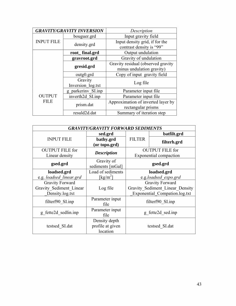
GRAVITY/GRAVITY INVERSION Description bouguer.grd Input gravity field

INPUT FILE density.grd Input density grid, if for the contrast density is “99”

root_ final.grd Output undulation gravroot.grd Gravity of undulation

gresid.grd Gravity residual (observed gravity minus undulation gravity)

outg0.grd Copy of input gravity field Gravity

Inversion_log.txt Log file

g_parkerinv_SI.inp Parameter input file inverth2d_SI.inp Parameter input file

prism.dat Approximation of inverted layer by rectangular prisms

OUTPUT FILE

resuld2d.dat Summary of iteration step

GRAVITY/GRAVITY FORWARD SEDIMENTS sed.grd batfilt.grd

INPUT FILE bathy.grd (or topo.grd)

FILTER filterh.grd

OUTPUT FILE for Linear density Description OUTPUT FILE for

Exponential compaction

gsed.grd Gravity of sediments [mGal] gsed.grd

loadsed.grd e.g. loadsed_linear.grd

Load of sediments [kg/m2]

loadsed.grd e.g.loadsed_expo.grd

Gravity Forward Gravity_Sediment_Linear

_Density.log.txt Log file

Gravity Forward Gravity_Sediment_Linear_Density_Exponential_Compation.log.txt

filterf90_SI.inp Parameter input file filterf90_SI.inp

g_fette2d_sedlin.inp Parameter input file g_fette2d_sed.inp

testsed_SI.dat Density depth

profile at given location

testsed_SI.dat

44

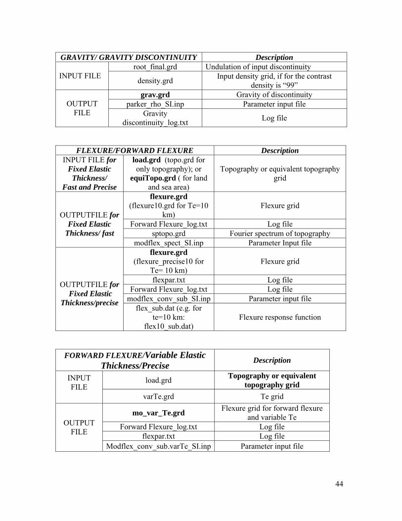
FLEXURE/FORWARD FLEXURE Description INPUT FILE for

Fixed Elastic Thickness/

Fast and Precise

load.grd (topo.grd for only topography); or

equiTopo.grd ( for land and sea area)

Topography or equivalent topography grid

flexure.grd (flexure10.grd for Te=10

km) Flexure grid

Forward Flexure_log.txt Log file sptopo.grd Fourier spectrum of topography

OUTPUTFILE for

Fixed Elastic Thickness/ fast

modflex_spect_SI.inp Parameter Input file flexure.grd

(flexure_precise10 for Te= 10 km)

Flexure grid

flexpar.txt Log file Forward Flexure_log.txt Log file

modflex_conv_sub_SI.inp Parameter input file

OUTPUTFILE for

Fixed Elastic Thickness/precise

flex_sub.dat (e.g. for te=10 km:

flex10_sub.dat) Flexure response function

FORWARD FLEXURE/Variable Elastic Thickness/Precise

Description

load.grd Topography or equivalent topography grid

INPUT FILE

varTe.grd Te grid

mo_var_Te.grd Flexure grid for forward flexure and variable Te

Forward Flexure_log.txt Log file flexpar.txt Log file

OUTPUT FILE

Modflex_conv_sub.varTe_SI.inp Parameter input file

GRAVITY/ GRAVITY DISCONTINUITY Description root_final.grd Undulation of input discontinuity

INPUT FILE density.grd Input density grid, if for the contrast density is “99”

grav.grd Gravity of discontinuity parker_rho_SI.inp Parameter input file

OUTPUT

FILE Gravity discontinuity_log.txt Log file

45

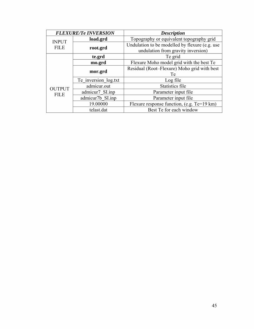
FLEXURE/Te INVERSION Description load.grd Topography or equivalent topography grid INPUT

FILE root.grd Undulation to be modelled by flexure (e.g. use undulation from gravity inversion)

te.grd Te grid mo.grd Flexure Moho model grid with the best Te

mor.grd Residual (Root–Flexure) Moho grid with best Te

Te_inversion_log.txt Log file admicur.out Statistics file

admicur7_SI.inp Parameter input file admicur7b_SI.inp Parameter input file

19.00000 Flexure response function, (e.g. Te=19 km)

OUTPUTFILE

telast.dat Best Te for each window

46

REFERENCES

Braitenberg, C., Ebbing, J. and Götze, H.J., 2002. Inverse modelling of elastic thickness

by convolution method - the eastern Alps as a case example. Earth and Planetary Science Letters, 202(2): 387-404.

Braitenberg, C., Wienecke, S. and Wang, Y., 2006. Basement structures from Satellite Derived Gravity Field: the South China Sea Ridge Journal of Geophysical Research-Solid Earth, 111: B05407.

Parker, R. L. 1972: The rapid calculation of potential anomalies. Geophys. J. R. Astr. Soc., 31, 447-455.

Tsikalas, F., 1992. A study of seismic velocity, density and porosity in Barents Sea wells (N. Norway). Master Thesis, University of Oslo - UIO, Oslo, Norway.

Wienecke, S., 2006. A new analytical solution for the calculation of flexural rigidity: significance and applications. PhD Thesis, http://www.diss.fu-berlin.de/2006/42 Free University Berlin, Berlin, 126 pp.

The grids in this tutorial were plotted with Golden Software Surfer.

Documents

Lithoflex tutorial 13giugno - Welcome to LithoFLEX.org lithoflex tutorial introduction 2 free mapping software geosoft 3 data format 3 data description / dummy values 4 study area