Embed Size (px)
Citation preview
Liquidity, Risk, and Occupational Choices∗
Milo Bianchi† Matteo Bobba‡
July 2012
Abstract
We explore which financial constraints matter most in the choice of becoming
an entrepreneur. We consider a randomly assigned welfare program in rural Mex-
ico and show that cash transfers significantly increase entry into entrepreneurship.
We then exploit cross-household variation in the timing of these transfers and find
that current occupational choices are significantly more responsive to the transfers
expected for the future than to those currently received. Guided by a simple occu-
pational choice model, we argue that the program has promoted entrepreneurship
by enhancing willingness to bear risk as opposed to simply relaxing current liquidity
constraints.
Keywords: Financial constraints; entrepreneurship; insurance; liquidity.
JEL codes: O16, G20, L26.
∗We thank four referees and especially Imran Rasul (Editor) for detailed and constructive comments.We also thank Orazio Attanasio, Abhijit Banerjee, Francois Bourguignon, Pierre Dubois, Eric Edmonds,Paul Glewwe, Marc Gurgand, Seema Jayachandran, Erik Lindqvist, Sylvie Lambert, Jean-Marc Robin,Jesper Roine, Mark Rosenzweig for useful comments and Christian Lehmann for research assistantship.The financial support of Region Ile-de-France and of the Risk Foundation (Groupama Chair) is gratefullyacknowledged.†Universite Paris-Dauphine; E-mail: [email protected]‡Inter-American Development Bank; E-mail: [email protected]
1
1 Introduction
Entrepreneurship is considered a fundamental aspect of the process of development (Haus-
mann and Rodrik [2003]; Ray [2007]; Naude [2010]), but one that is often hindered by
financial constraints (Banerjee and Duflo [2005]; Levine [2005]). One way in which access
to finance may promote economic development is by providing some poor individuals the
opportunity to set up their own businesses (Banerjee [2003]; Karlan and Morduch [2009]).
Understanding the link between improved access to finance and occupational choices,
however, poses some serious challenges. First, such an improvement seldom occurs in
isolation from other changes in the economy, which makes it hard to estimate empirically
its effects. Moreover, and perhaps even more fundamentally, occupational choices may be
determined by several financial constraints, such as those concerning households’ ability
to save, borrow and obtain insurance against income shocks. Hence, one would like
to open the box of “access to finance” and understand which of the various financial
constraints is binding in a given situation. This is often complicated but obviously key
for the interpretation of the effects and the design of effective policies.
This paper takes a step along these lines by asking whether financial constraints matter
and which financial constraints matter most in the choice of becoming an entrepreneur.
We first show that some individuals become entrepreneurs after receiving a positive shock
to their households’ income. We next analyze whether this effect is due to improved access
to start-up capital or rather to an improved ability to insure against entrepreneurial risk.
We develop a simple model to highlight how liquidity and insurance constraints respond
differently to the time profile of expected income shocks. We then exploit the variation
in the timing of these shocks in order to evaluate the relative importance of these two
constraints in our setting.
More specifically, we exploit the welfare program Progresa, which targets poor house-
holds in rural Mexico and provides cash transfers conditional on their behaviors in health
and children’s education. While Section 2 provides a more detailed description of the
program, we here stress some features which make it interesting for our exercise. First,
the timing of access into Progresa has been randomized, thereby providing us a reliable
control group to estimate its effects on occupational choices. Second, transfers are ad-
ministered for an extended and predictable time period and, albeit partly conditional
on schooling behaviors, they typically represent a sizable increase in households’ wealth.
Moreover, and perhaps most importantly for our purposes, their magnitude and time
profile vary substantially according to household demographics; as a result, households
face different (and partly exogenous) shocks to their current liquidity and to their ability
to insure against future income fluctuations.
2

We first compare households in treated and control communities; we show that being
entitled to the program’s cash transfers significantly increases the probability of enter-
ing self-employment. This provides (indirect) evidence that individuals face financial
constraints in the decision to become entrepreneurs. We then exploit the fact that, as
mentioned, treated households face different time profiles of cash transfers. In particular,
the educational scholarship they are entitled to receive in a given year varies substantially
with the number, grade in school and gender of their children. Slight cross-household vari-
ations in these characteristics might induce significant differences in the amount of current
and future transfers. We then ask whether the choice of becoming an entrepreneur in the
current period is more responsive to the transfers currently received or to those expected
for the future.
We motivate our analysis by developing a simple occupational choice model in which
individuals may face liquidity or insurance constraints. If wealth cannot be freely allo-
cated across periods, since for example households cannot borrow, current and future
transfers have different effects on the choice of becoming an entrepreneur. The transfers
currently received are better suited to meeting start-up costs and thus are more impor-
tant if liquidity constraints are binding. Conversely, future transfers are better suited to
providing insurance against business failure and thus have stronger effects if insurance
constraints are binding.
We then show that the probability of becoming an entrepreneur in the current period
is significantly more responsive to the amount of transfers expected for the near future
than to the amount currently received. This result is robust in various specifications, in
which we control for the total amount of transfers received within a given time horizon.
We also rule out that the very same household characteristics which determine the profile
of transfers determine occupational choices as well.
In our view, these results tend to support the hypothesis that the program has been
effective in promoting entrepreneurship, as it has relaxed insurance constraints as opposed
to simply relaxing current liquidity constraints. While one may think of alternative stories
whereby both current and future transfers matter (for example, future transfers may be
used as collateral for moneylenders; or future investments may be needed to keep up with
business needs), it is hard to explain that future transfers matter more based on liquidity
constraints.
In order to obtain further support in favor of this interpretation, we construct a mea-
sure of entrepreneurial risk based on the variance of pre-program income of entrepreneurs
relative to salaried workers in each village. We show that individuals are less likely to
become entrepreneurs in villages where entrepreneurial returns are more volatile; and,
indeed, these are the villages in which the treatment has the largest effects. These results
3
are robust to various definitions of the geographic scope of the relevant local market.
Based on this evidence, we argue that financial barriers to entry into self-employment
do not appear as the most important obstacle in our setting (see McKenzie and Woodruff
[2006] for similar evidence on micro-enterprises in urban Mexico). Instead, the possibility
of better insuring against future income fluctuations may be what induces some individ-
uals to undertake the risky choice of setting up a business.
We conclude our analysis with an exploration of the medium-term effects of the pro-
gram on entrepreneurship. By exploiting an additional evaluation survey conducted six
years after the start of the program, we show that the entrepreneurial dynamics induced
by Progresa may have a persistent effect. In particular, in villages with a lower pre-
program share of entrepreneurs, the exposure to Progresa’s transfers is associated with
significantly higher rates of entrepreneurship after some years.
Related literature This paper builds on the literature on improved access to finance
and occupational choices. Exploiting income shocks, Holtz-Eakin et al. [1994] and Blanch-
flower and Oswald [1998] show that having received an inheritance increases the proba-
bility of being or remaining self-employed. In experimental settings, de Mel et al. [2008]
consider a sample of individual who already have a business in Sri Lanka and show that
a random prize in cash or in kind considerably boosts their profits. More broadly, a sub-
stantial literature has explored the effects of improved access to credit and to insurance
(see, e.g., Besley [1995] and Banerjee [2003] for reviews). Experimental evidence along
these lines is, however, still scarce and very recent. Banerjee et al. [2009] and Karlan
and Zinman [2010] provide evidence on the impact of micro-credit on small businesses in
India and in the Philippines, respectively. Gine et al. [2008], Gine and Yang [2009] and
Cole et al. [2012] study the determinants of take-up of weather insurance in Malawi and
India. Differently from our setting, they directly explore the importance of risk aversion
by eliciting responses to a specific survey. In general, however, despite liquidity and in-
surance constraints are often interrelated (Ray [1998]), little has been done to attempt
to separate their effects. One notable exception is Dercon and Christiaensen [2011], who
distinguish seasonal credit constraints from inter-temporal constraints related to risk on
fertilizer adoption in Ethiopia.
There is also a substantial body of research related to Progresa and its experimental
design, but to our knowledge no study has explicitly looked at its effects on occupational
choices. The most closely related paper in this literature is Gertler et al. [2012]. They
document that Progresa’s transfers were partly used to increase investments in agricul-
tural assets and in business activities (which may or may not coincide with the main
occupation) and that as a result the program has long-lasting effects on the welfare of
4

its beneficiaries. While the starting point of our paper is related, as we also show that
Progresa induced households to change their income generating activities, the main focus
is quite different. Gertler et al. [2012] are interested in the impact of the program on
long-term living standards. At the same time, as they acknowledge, their effect may
be driven both by relaxed liquidity and insurance constraints. The authors provide no
attempt to distinguish the two mechanisms, which is instead the main focus of our paper.
2 Background and Data
2.1 Program Description
Launched in Mexico in 1997, Progresa is a large-scale welfare program mainly aimed at
improving health and human capital accumulation in the poorest rural communities.1 It
provides households with conditional cash transfers targeted to specific behaviors in nutri-
tion, health and education. Initially, 506 villages were selected to be part of the program
evaluation sample. Within those, 320 villages were randomly allocated to the treatment
group and 186 villages to the control group. As we show in Table 1, randomization has
been successful in attaining balanced treatment and control populations. Among several
individual, household and village characteristics, none displays statistically significant
baseline differences.
Households are classified as eligible for the program if their poverty index, assessed
using information collected before the start of the program, is above a given threshold.
Importantly for our analysis, the eligibility status was fixed for the entire duration of the
program (and so insensitive to subsequent changes in asset holdings).2 Eligible households
in treatment communities started receiving benefits in March-April 1998, whereas eligible
households in control communities were not incorporated until November 1999. Cash
transfers from Progresa are given bimonthly and come in two forms. The first is a fixed
food stipend of 105 Pesos per month conditional on family members obtaining preventive
medical care.3 The second is an educational scholarships which is provided for each
child who is less than 18 years old and enrolled between the third and the ninth grade,
conditional on attending school a minimum of 85 percent of the time and not repeating
a grade more than twice. Scholarship amounts range from 81 to 269 Pesos per month
1The program is currently ongoing under the name Oportunidades.2As an exception to this rule, around 3,000 households (the so-called densificados) were classified as
non-poor in the baseline but were later reclassified as eligible. In order to avoid arbitrary classifications,we exclude those households from our analysis (the results are unchanged, though, once we includethem).
3These figures are expressed in current Pesos as of the second semester of 1998. Transfer size hasbeen increased over time in order to adjust for inflation.
5

per child; they increase with school grade and, in seventh to ninth grades, are larger for
girls than for boys.4 Overall transfer amounts can be substantial: median benefits are
176 Pesos per month (roughly 18 USD in 1998), equivalent to about 28% of the monthly
income of beneficiary families.
2.2 Sample Description
In our main empirical analysis, we exploit a baseline survey conducted in October 1997
and a series of Household Evaluation Surveys collected every six months starting in Octo-
ber 1998 for a total of five waves after the baseline.5 These surveys include socioeconomic
characteristics at the individual level for 24,077 households, of which about 53% are clas-
sified as eligible. We mostly focus on eligible households during the experimental period:
in addition to the baseline, we employ the first three waves of the follow-up surveys
conducted in October 1998, March 1999 and October 1999.6 Program take-up is high
in this sample: 86% of the treated households are reported to have received positive
transfers within 18 months since program offering. Sample attrition is low (11%), and
non-response in occupational choice somewhat larger (17%); however, neither is related
to the treatment assignment.
In the baseline, we have information on the main occupation of 20,770 eligible adult
individuals (18 years old or more). We mainly concentrate on flows into entrepreneurship,
i.e., on those individuals who are either salaried or report no paid occupation (we refer
to them as unemployed) in the baseline and who become entrepreneurs in the follow-up
period. Among those residing in control villages, 4% become entrepreneurs during this
period (mostly self-employed), of which roughly 25% were unemployed in the baseline
and 20% are women.
A distinctive features of new entrepreneurs is their engagement in micro-business
activities not (directly) related to agriculture. In control villages, 11% of new en-
trepreneurs report being engaged in activities like carpentry, handicraft, and domestic
services, whereas the corresponding share for salaried workers is only 3%. Moreover,
we note that 34% of new entrepreneurs in control villages have more than one paid oc-
cupation vis-a-vis 8% of salaried workers. This is common in many developing settings,
4Specifically, a household is entitled to receive 81 Pesos per month for each child enrolled in the thirdgrade. The corresponding amounts for the following grades are respectively 91, 116, 146, 214, 224 and239 for males and 91, 116, 146, 224, 249 and 269 for females. In our sample period, no educationaltransfers are given before the third grade or after the ninth grade.
5A second baseline survey was conducted in March 1998, but it did not contain any question aboutoccupational status.
6We employ the survey waves of March 2000 and November 2000 as one placebo sample in Section 3.In Section 6 we use an additional survey wave collected in 2003 to study the medium-term effects of theprogram.
6
and it is typically interpreted as an income smoothing strategy (see, e.g., Morduch [1995],
Banerjee and Duflo [2008]). Indeed, also in our sample, new entrepreneurs face a substan-
tially higher volatility of labor income in their primary occupation, which may increase
their need for self-insurance.7
3 Entrepreneurship and Financial Constraints
3.1 Program Impacts
Consider an individual i who is either a salaried worker or unemployed in the baseline,
and let nei,t be a dummy equal to one if the individual has become an entrepreneur in
a given program period t and zero otherwise. We estimate regressions of the following
form:
nei,t = α1Tl +X ′i,t0α2 + εi,t, (1)
where Tl represents the Progresa treatment assignment at the locality level l and the
vector Xi,t0 denotes a set of pre-determined covariates: individual age, gender, educa-
tion, income, spouse’s main occupation, household wealth and demographic composition,
village shares of entrepreneurs and proxies for agricultural risk. We also include time
dummies and state dummies.8 In order to take into account the potential intra-village
correlation of the individual error term εi,t, we cluster standard errors at the village level.
Table 2 reports OLS estimates of α1 in equation (1), which measures the average effect
of eligibility for Progresa transfers on the transition into entrepreneurship.9 Program
impacts appear to be both statistically and economically significant. As shown in column
(1), being entitled to the program increases the probability of entering self-employment by
0.9 percentage points. In relative terms, this represents an increase of 24% with respect
to the counterfactual sample averages (equal to 4%). In columns (2)-(3), we show that
the program significantly increases the probability of entry into entrepreneurship from
both salaried work and unemployment.
In order to explore whether the above results are driven by receiving program benefits,
we run two additional tests. First, we estimate equation (1) for periods in which control
villages are incorporated into the program (corresponding to the survey waves of March
2000 and November 2000). As shown in column (4), there are no significant treated-
control differences in the probability of entry into entrepreneurship when both treated
7The standard deviation of monthly labor income in control villages is 84% of the sample mean forentrepreneurs vis-a-vis 60% for salaried workers.
8We cannot specify fixed effects at a more disaggregated geographical level, such as municipality orvillage, since this would imply losing the exogenous variation induced by the experiment.
9All our results are robust if we use a Probit model instead.
7

and control villages are receiving the transfers. Second, we estimate equation (1) on
individuals who are not classified as poor and so are not eligible to receive the transfers.
As shown in column (5), there are no significant treated-control differences for these
individuals.
3.2 Alternative Channels
As described in Section 2, cash transfers are conditional on health and schooling behav-
iors. In particular, the requirement of sending children to school may have a direct effect
on occupational choices: for example, as children become less likely to work at home,
adults may have to quit a salaried job and turn to self-employment in search of flexible
working hours. According to this interpretation, treatment impacts should be higher for
those households who change their schooling behaviors in response to the program, either
by enrolling children who were not enrolled before the program or by keeping enrolled
children in school longer. As for the former group, we construct a dummy equal to one
if the household has eligible children not enrolled in school at the baseline. In order to
account for the second possibility, we construct two dummy variables: the first is equal
to one if the household has eligible children enrolled in the last two grades of primary
school at the baseline; the second is equal to one if the household has eligible female
children enrolled in the first two grades of secondary school at the baseline. According
to Schultz [2004], the program indeed has a greater impact on the transition between
primary and secondary school and on female secondary schooling. In columns (1)-(3) of
Table 3, we report that program impacts do not seem to vary along these dimensions.
Alternatively, Progresa may change parents’ expectations about their children’s school
trajectories, and this may directly impact adults’ occupational choices. In this case, our
effects may be concentrated on adults reporting lower expectations at the baseline. We
then interact our program treatment indicator with pre-program parents’ expectations
about their children’s educational attainments.10 Again, we see no systematic differences
in program impacts with respect to these expectations (column 4).
A different explanation of our findings is based on the potential complementary be-
tween Progresa and preexisting programs. Indeed, in our sample villages, households
may also benefit from welfare programs which are directly related to their occupational
choices.11 If Progresa improves the effectiveness of these programs, the observed changes
10Specifically, parents are asked which grade they think each of their children can attain. We takethe average of these grades for each households and construct a dummy equal to one if the householdreports average expected attainment above secondary school, which corresponds to the sample median,and zero otherwise.
11In particular, Probecat and Cimo, which provide training grants to the unemployed and to thoseemployed in small firms; Programa de Empleo Temporal, which provides temporary employment in publicprojects; and Procampo, which provides subsidies to rural workers.
8
in occupational choices may be only spuriously related to Progresa’s transfers. In this
case, we expect effects to be concentrated among households who are also beneficiaries of
alternative programs. We then interact our program treatment indicator with a dummy
equal to one if the household has received money from any of these programs during the
sample period. As shown in column (5), the data do not suggest that our effects are
mediated by complementary welfare programs.12
Taken together, this evidence lends support to the view that Progresa has affected
individuals’ occupational choices due to the provision of monetary benefits rather than
through other behavioral responses to the program. This suggests that individuals face
financial constraints in their decision to become entrepreneurs. We then try to better
uncover the nature of these financial constraints.
4 Liquidity and Insurance Constraints: Theory
Absent the program, individuals may refrain from becoming entrepreneurs for at least two
reasons. First, they may face liquidity constraints which prevent them from undertaking
some initial capital investment. The program would then promote entrepreneurship by
increasing their current liquidity. Second, individuals may prefer avoiding the risk associ-
ated with entrepreneurial returns. In this case, by providing transfers for an extended and
predictable period of time, the program would promote entrepreneurship by increasing
individuals’ ability to cope with future income fluctuations. In this section, we develop a
simple model to highlight how liquidity and insurance constraints respond differently to
the time profile of expected income shocks.
Setup Consider a population of individuals who are heterogeneous in their initial wealth
a and in their risk aversion r. Individuals live for two periods. In the first period,
they choose their occupation: either they become self-employed, which requires a fixed
investment of k units of capital, or they look for a salaried job. In addition, they choose
the amount of wealth they wish to save (possibly as a function of their occupational
choice), which we denote as s. We do not allow for borrowing and so impose
s ≥ 0, (2)
12Alternatively, we interact our program indicator with a dummy equal to one if the household hasreceived money from any welfare program (as opposed to only those directly related to occupationalchoices) and with the total amount of money received from those programs. The results are very similarto those reported in column (5).
9

and we normalize the returns of saving to one.13
In the second period, individuals enjoy the returns from their occupation. The self-
employed get y with probability p and zero otherwise. Among those who look for a
salaried job, a fraction λ finds one while the rest remains unemployed. In the former case,
individuals get a fixed wage w, while if unemployed they enjoy benefits b, with b ≤ w.
We assume that py − k ≥ λw + (1 − λ)b and p ≤ λ, which imply that self-employment
has higher expected returns but higher risk than looking for a job.
Savings and occupation are chosen in order to maximize
U = u(x1) + E[u(x2)],
where E[·] is the expectation operator and x1 and x2 denote consumption in period 1 and
2. We assume that u exhibits decreasing absolute risk aversion, and for simplicity we
abstract from time discounting.
Finally, irrespective of their choices, individuals are entitled to cash transfers C1 in
period 1 and C2 in period 2. Our main interest is in exploring how the share of self-
employed varies with the transfers C1 and C2. We here provide an intuitive argument; a
more detailed exposition can be found in the Appendix.
Analysis As is standard in this class of models (see e.g. Kihlstrom and Laffont [1979]),
there exists a threshold level of risk aversion r∗ such that those with r ≤ r∗ prefer being
self-employed. The self-employed are then defined as those individuals with r ≤ r∗ and
a+ C1 ≥ k.
Consider first those individuals for whom borrowing constraints do not bind. With
simple algebra, it can be shown that their occupational choice is equally responsive to C1
and to C2. As is intuitive, individuals who can optimally allocate wealth across periods
see no fundamental difference between transfers received today and those they know they
will receive in the future.
Suppose, however, that for some agents borrowing constraints are binding. In this
case, current and future transfers are not equivalent. To see this, consider first a world
with only liquidity constraints. That is, suppose that k > C1 and individuals are risk
neutral, so that all those with a + C1 ≥ k become self-employed. In this setting, the
share of self-employed in period 1 is more responsive to C1 than to C2. The reason is
that current transfers help overcoming liquidity needs while future transfers may not be
pledged for obtaining cash in period 1 and finance the investment k.
Consider now a world in which there are only insurance constraints. That is, suppose
13Borrowing constraints are widely documented (restricting to developing countries, see the surveys inBanerjee [2003] and Karlan and Morduch [2009]).
10
that k ≤ C1 and individuals are risk-averse, so that all those with r ≤ r∗ become self-
employed. In order to be willing to take risk, individuals need to have enough wealth
in period 2, and this is in turn more likely to occur by increasing C2 than by increasing
C1. The reason is that individuals with binding borrowing constraints consume all their
wealth in the first period (and still they would prefer consuming more); hence, increasing
C1 does not make them richer in period 2 and so does not affect their willingness to take
risk. As a result, self-employment is more responsive to future than to current transfers.
We then have the following Proposition.
Proposition 1 Suppose individuals face constraints on allocating transfers across peri-
ods. Then current occupational choices are more responsive to the size of current transfers
if liquidity constraints bind, while they are more responsive to the size of future transfers
if insurance constraints bind.
Remark The previous model abstracts from working capital. Yet, if future capital
investments were needed, future transfers would matter even in a world without risk. To
see this most simply, suppose that the self-employed need to invest k1 in period 1, k2 in
period 2 and they gain π3 in period 3. Suppose payoffs are deterministic and such that
self-employment is more profitable than salaried work. If k2 ≥ C2, future transfers are
indeed important as they help to meet future liquidity needs. However, in this setting,
future transfers cannot matter more than current transfers. In fact, individuals who
invest in period 1 have a + C1 ≥ k1, and so they would always be able to save should
that be necessary to pay k2. Hence, both increasing C1 and increasing C2 would have the
same effect on helping them to finance period 2 investment and so become self-employed.
5 Liquidity and Insurance Constraints: Evidence
In this section, we empirically explore the mechanisms outlined above by taking advantage
of a second source of variation. As described in Section 2, treated households differ in
the magnitude and time profile of the transfers they are entitled to, as determined by the
number, grade in school and gender of their children. We can then test how individual
i’s probability of becoming an entrepreneur at time t depends on the cumulative amount
of transfers received by the household in the previous period and on the transfers known
to be received in the next period.
11

5.1 Empirical Strategy
In what follows, we restrict our attention to eligible individuals who reside in treated
villages. In order to take the theoretical predictions to the data, we need to specify
the time span of “current” and “future” periods. Given the structure of the program,
individuals are entitled to receive transfers for several years. Nonetheless, we wish to focus
on transfers to be received in the near future. The further away are future transfers, the
more confounded their impact on occupational choices may be, so it may be more difficult
to relate current occupational choice to the transfers to be received in a few years than to
those to be received in a few months.14 At the same time, the chosen time period cannot
be too short. Since transfers vary with the school calendar year, future transfers need
not be systematically different from current transfers if we consider a period shorter than
six months. For these reasons, in most of our analysis, we focus on a six-month period.
In robustness checks, we consider different time horizons.15
Beside being possibly measured with error, the actual amounts received partly depend
on households’ behaviors in complying with the program’s conditions, and these are likely
to be simultaneously determined with occupational choices. We thus define potential
transfers Ph,t and Ph,t+1 as the amount of transfers a household would be entitled to,
according to the rules described in Section 2, assuming that its children did not change
their pre-program enrollment decisions and, when enrolled, progressed by one grade in
each year. These transfers are deterministic functions of children’s characteristics at the
baseline and by construction they are uncorrelated with any behavioral response to the
program.
Motivated by Proposition 1, we then consider (variations of) the following empirical
model:
nei,t = β1Ph,t+1 + β2 [Ph,t+1 + Ph,t] + Child′h,tβ3 + ηi,t. (3)
Our coefficient of interest is β1, which measures the differential impact of future vs.
current transfers on the probability of becoming an entrepreneur (i.e. ∂nei,t/∂Ph,t+1 −∂nei,t/∂Ph,t). The vector Childh,t contains age-specific categorical variables for the num-
ber of boys and girls who are between 6 and 17 years old in each household h and post-
14In addition, unreported results show that for those who become entrepreneurs in survey wave t,there is a drop in expenditures and consumption in wave t and a recovery already in wave t+ 1, which issix months afterward. This suggests that the time lag between the occupational choice and its (initial)payoffs, which corresponds to period 1 and period 2 in our model, is less than six months.
15Since we do not know exactly the date on which individuals have changed occupation between twosurvey waves, current and future transfers are constructed by taking the month of the interview asthe reference. It follows that our future amounts are certainly received after individuals have changedoccupation, while part of our current amounts may sometimes still be due at the time in which theyswitch occupation. If this were the case, our estimates on the differential effects of future vs. currenttransfers should be interpreted as a lower bound.
12
treatment period t, which controls for any independent effect of children demographics on
occupational choices. In order to take into account potential intra-household correlation,
standard errors are clustered at the household level.
In equation (3), both the level and the time profile of potential transfers may vary
across households with identical compositions in terms of children age and gender since
these children may differ in their attainment level or enrollment status at the baseline.
Indeed, in terms of attainment, due to grade repetition and/or early enrollment in school,
on average 65% of the students enrolled within the seven program grades are either
younger or older than they would be had they started school at the age of six and
proceeded thereafter without setback. Also, in terms of enrollment status, about 90%
of children at the baseline are enrolled at the primary level, but only 60% of the boys
and 48% of the girls are enrolled at the junior secondary level. Notice also that, since
households typically have several eligible children, in many instances these sources of
variations in transfers may co-exist within the same family.16
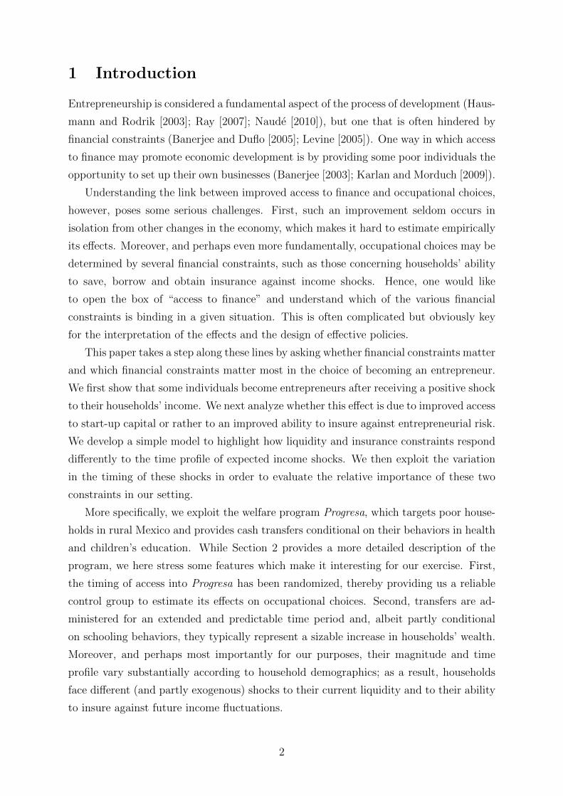
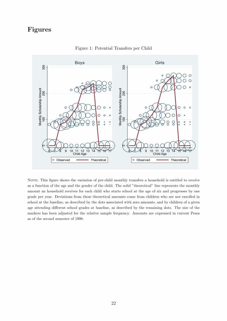
These patterns are represented in Figure 1, which reports a scatter plot of per-child
monthly educational transfers a household is entitled to receive as a function of the age,
gender and baseline schooling status of the child. As described in Section 2, monthly
scholarships amount to 81 Pesos per child enrolled in the third grade, and they increase
for each grade up to the ninth. Hence, a child who starts school at the age of six and
progresses by one grade per year is entitled to receive 81 Pesos at the age of eight and
then an increasing amount of transfers up to age fourteen. This is represented by the solid
line which we call “theoretical”. Deviations from these theoretical amounts come from
children who are not enrolled in school at the baseline, as described by the dots associated
with zero amounts, and by children of a given age attending different school grades at
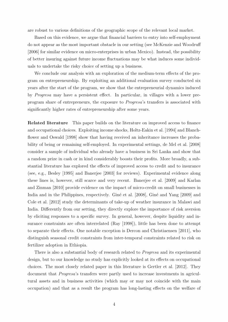
the baseline, as described by the remaining dots. Moreover, as documented in Figure 2,
cross-household differences in children demographics and their baseline schooling status
induce considerable variations in the time profile of potential transfers, which indeed
allow us to separately identify β1 and β2 in equation (3).
5.2 Results
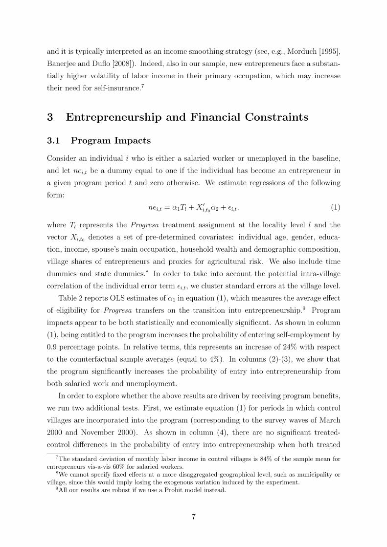
We first provide a visual inspection of our relationships of interest. In Figure 3, we
plot the effects of current and future transfer amounts on the probability to become an
entrepreneur, estimated with non-parametric local linear regressions. The shape of the
curves suggests that the amount of transfers received in the previous six months does not
have any effect on the probability of becoming an entrepreneur. On the contrary, this
16On average, households who are entitled to the educational scholarship have 3.5 children (less than18 years old), of which about 2 are eligible to receive the scholarship in a given year.
13

probability seems to depend positively on the amount of transfers that households are
entitled to receive in the next six months.
These patterns are confirmed in the OLS estimates reported in Table 4. Column (1)
displays the results for the amounts received in the previous six months, which reveal no
significant effects. According to column (2), instead, the effect of the transfers a household
is entitled to receive in the next six months appears significant and large: a one-standard
deviation increase in future transfers increases the average probability of becoming an
entrepreneur by 0.5%.17 This amounts to an 11% increase vis-a-vis the average share
of new entrepreneurs in this sample (4.6%). We then directly estimate the differential
impact of current vs. future transfers, as measured by the coefficient β1 in equation (3).
As reported in column (3), the estimated coefficient is positive and significant, which
shows that the probability of becoming an entrepreneur is significantly more responsive
to the amount of future transfers than to the amount of current transfers.
A key issue in the interpretation of the above findings is that the underlying rela-
tionship between occupational choices and households characteristics may confound the
effects of transfer amounts.18 Our key identifying assumption is that, absent the pro-
gram, occupational choices respond to children’s demographics and not to their baseline
attainment level or enrollment status. We test this assumption by looking at two al-
ternative samples: program-eligible households living in control villages and non-eligible
households living in treated villages. We construct the transfers they would have been
entitled to had they been treated, and estimate the effect of these placebo potential trans-
fers on occupational choices. As shown in columns (4) and (5) of Table 4, there are no
effects of Ph,t+1 and Ph,t in these samples. This allows us to interpret the estimates in
columns (1)-(3) as the result of the transfers induced by Progresa and not of the specific
household characteristics which determine them.
We further perform some specification checks. We first investigate whether our es-
timates may be driven by some underlying relationship between the total amount of
transfers received and to be received from the program and their time profile over a
six-month horizon. In column (1) of Table 5, we consider the total amount of transfers
potentially received between March 1998 and September 2000. This corresponds to the
longest time period for which we can compute potential transfers without making further
assumptions on the schooling decisions of those who were five years old at the baseline.
The coefficient associated with total amounts is very small and not significant (as one
would expect in a setting in which future wealth cannot be pledged for current wealth),
17The average potential transfers received in the past six months are 1,448 Pesos (std. dev. 856) andthe average potential transfers to be received in the next six months are 1,548 Pesos (std. dev. 954).
18If the very same characteristics which determine the profile of transfers also determine occupationalchoices, it would not be possible to separately estimate the two in equation (3).
14
while the estimated coefficient on the differential impact of future vs. current transfers
barely changes.19 In columns (2) and (3), we check the robustness of our findings with
respect to the definition of transfer horizon. We consider households’ response to trans-
fers which have been received in the past year and to those to be received in a year (as
opposed to six months as in our main specification). The results are consistent with the
previous ones: current transfers do not matter while future transfers do, even though
estimates tend to be less precise (as one would expect, the longer the transfer horizon
the noisier our relation of interest). In magnitude, the relative effects for one-year future
transfers are comparable to those for six months: a one-standard deviation increase leads
to 0.4% more self-employed, which corresponds to a 9% increase.
These results suggest that the time profile of the transfer is key for explaining occu-
pational choices in this setting. Based on our previous occupational choice model, this
can be interpreted as evidence of binding insurance constraints, whereby cash transfers
promote entrepreneurship by making individuals more willing to take risks as opposed to
simply allowing them to incur some start-up investment.
In order to gain further support for this interpretation, we construct a measure of the
risk that entrepreneurs face in their local market. The variable Risk(village) is defined
as the ratio of the variance of labor income for the entrepreneurs vs. salaried workers at
the village level, based on pre-program income statements. As the relevant local market
need not coincide with the village (for example, entrepreneurs could trade in neighboring
villages), we construct a similar measure based on the relative variance of entrepreneurial
income in other evaluation villages situated within 10 kilometers of each village.20 As
we see in columns (4)-(5) of Table 5, irrespective of the definition of the relevant local
market, individuals are significantly more reluctant to become entrepreneurs in areas
where entrepreneurial returns are more volatile. These are indeed the settings in which
the treatment appears to have the largest effects on occupational choices.
6 Medium-Term Impacts
Our previous analysis focused on the short-term impact of the program on the probability
to become entrepreneur. A key question for a broader understanding of the effects of the
19This result is robust to alternative definitions of total transfers. For example, we have considered a(rough) measure of the total income shock a household expects to receive in the long run based on itsbaseline composition (including children of all ages and making standard assumptions on their schoolingbehavior).
20We define neighborhoods using simple geodesic distances from each evaluation village. In our sample,80% of the villages have at least another evaluation locality situated within 10 kilometers. The averagevariance ratio within a village is 1.48 (std. dev. 1.99) and the average variance ratio within 10 kilometersfrom each village is 1.43 (std. dev. 1.79).
15

program transfers is whether Progresa induces persistent changes in entrepreneurial ac-
tivities. In our setting, this question can be addressed by exploiting an additional round
of the Household Evaluation Survey collected in 2003. While we cannot compare the orig-
inal treated and control groups (as the latter started receiving the program benefits since
November 1999), the survey contains information not only on the original 506 evaluation
localities but also on a new group of 152 localities that were not incorporated into the
program as of 2003. The new localities were selected so as to closely match the evaluation
localities according to a number of socioeconomic indicators (which include poverty lev-
els, demographic characteristics and labor market conditions). For the individuals who
reside in those communities, we rely on recall data on their socioeconomic characteristics
(including their main occupation) in 1997.21 We then obtain a longitudinal database of
17,661 program-eligible adult individuals. Among them, 66% are receiving the treatment
in 2003 (either since four or since five and a half years), while the remaining 34% represent
the new control group.
Households in the new control group come from different geographic areas than the
original evaluation sample. Hence, they may have experienced different (labor market)
conditions, and this may have affected their occupational choices. To take such differences
into account, we first compare longitudinal changes in the share of entrepreneurs between
localities in the original evaluation sample and in the new control group. More specifically,
we consider the following difference-in-differences specification:
el,t = γ1Tl + γ2dt + γ3[Tl × dt] + zl,t, (4)
where el,t is the share of entrepreneurs in village l in period t; Tl is a dummy equal to one
if locality l belongs to the original evaluation sample; dt is a dummy equal to one for the
2003 round of data and zero for the 1997 baseline. We also include state dummies and
cluster standard errors at the locality level to account for potential serial correlation.22
In this specification, γ1 captures any time-invariant difference between the two groups of
localities, γ2 any time trend which is common across groups, and γ3 measures the average
longer-term impact of the program on the local share of entrepreneurs.
We next compare individual transitions into entrepreneurship between 1997 and 2003
across the two groups. Since the new control group was selected according to socio-
21Retrospective data for 1997 were only collected in the new control communities, so we cannot directlycompare them with the actual information collected in 1997. Behrman et al. [2011], however, providesome indirect test of recall bias in this setting. We also notice that our subsequent results for the averageshare of entrepreneurs across villages require a somewhat weaker assumption than classical measurementerror; it suffices that any potentially non-classical recall error cancels out within each village.
22We weight each village-level observation by the relative population size in order to better comparethe resulting estimates with those at the individual level reported thereafter.
16

economic characteristics aggregated at the community level, we use matching methods to
take into account differences in the support and in the distribution of pre-program individ-
ual and household characteristics between the two groups. While analogous to standard
difference-in-differences, this approach does not impose functional form restrictions when
estimating the conditional expectation of the outcome variable, and it re-weights the ob-
servations according to individual probability (propensity) to participate in the program
(see, e.g., Heckman et al. [1998]). We refer to Appendix Table A.1 for standard indi-
cators of covariate balancing, and here only notice that the after-matching distribution
of the covariates is well balanced, thereby suggesting that the propensity score model is
correctly specified and the estimator is consistent.
We report our results in Table 6. Column (1) shows a small and non-significant effect
of the program on the village share of self-employed in 2003. This average estimate,
however, masks significant heterogeneity. We split the sample according to the local
share of entrepreneurs in 1997, based on whether the village share falls above or below the
median share. As reported in columns (2) and (3), the share of self-employed decreases in
treated communities with a higher pre-program share of entrepreneurs, while it increases
in those with a lower pre-program share. In columns (4) and (5), we show that these
results are qualitatively similar when estimating equation (4) with the matching procedure
outlined above. However, while the negative effect is smaller in magnitude and not
statistically different from zero, the positive effect remains statistically significant and
barely changes in magnitude. Among villages with a lower share of entrepreneurs in
1997, the treatment is associated with a 2.2% higher share of entrepreneurs in 2003.
One interpretation of this finding may build on a model in which new entrepreneurs
compete with existing entrepreneurs in satisfying a local demand (as, for example, in
Lucas [1978]). Our aim, however, is not to explore in detail the mechanisms behind
this result. Taking a more limited approach, we interpret it as evidence that the short-
run response to the program documented in the previous sections appears to have some
long-lasting effect on entrepreneurship, at least in a subset of villages in our sample.
7 Conclusion
We have explored the response of occupational choices to the income shocks induced
by the Mexican program Progresa. We have first documented that the probability of
becoming an entrepreneur increases by about 25% for treated individuals. We have
then shown that the time profile of the transfer is key to explaining these effects: current
occupational choices are significantly more responsive to the amount of transfers expected
for the future than to those currently received. Based on a simple occupational choice
17

model, we have interpreted these results as evidence that cash transfers have been effective
in promoting entrepreneurship, as they have induced individuals to take more risks as
opposed to simply relaxing current liquidity constraints.
Our results include some limitations. For example, we have not fully addressed the
possibility of general equilibrium effects induced by the program. As a first step, we
have shown that indirect effects on non-eligible households in treated communities are
not significant. However, much remains to be done on the extent to which the dynamics
described above affect the functioning of local markets (e.g., in terms of increased labor
demand or total production). Moreover, while in Section 6 we provide some evidence
that our effects may be persistent, a more general analysis of the long-run impacts of
Progresa’s cash transfers is left for further investigation.
Nonetheless, we think our analysis can inform the debate on financial constraints and
entrepreneurship in developing countries. First, while some skeptics question whether
policy makers can promote entrepreneurship at all (see, e.g., Holtz-Eakin [2000] and
Shane [2009] for a discussion), we have shown one instance in which this could be done.
Indeed, in line with the evidence in Gertler et al. [2012], it appears that Progresa’s cash
transfers had a significant impact on households’ income-generating activities. In addi-
tion, we have shown that liquidity constraints need not be a major barrier to entry into
entrepreneurship. Instead, individuals may refrain from entering self-employment be-
cause of its risky returns. In this view, promoting entrepreneurship may require reducing
households’ exposure to risk in other dimensions.
18

References
Banerjee, A. V. [2003], Contracting Constraints, Credit Markets, and Economic Develop-
ment, in ‘Advances in Economics and Econometrics: Theory and Applications: Eighth
World Congress’, Cambridge University Press.
Banerjee, A. V. and Duflo, E. [2005], Growth theory through the lens of development
economics, in P. Aghion and S. Durlauf, eds, ‘Handbook of Economic Growth’, Vol. 1
of Handbook of Economic Growth, Elsevier, chapter 7, pp. 473–552.
Banerjee, A. V. and Duflo, E. [2008], ‘What is middle class about the middle classes
around the world?’, Journal of Economic Perspectives 22(2), 3–28.
Banerjee, A. V., Duflo, E., Glennerste, R. and Kinnan, C. [2009], ‘The miracle of micro-
finance? evidence from a randomized evaluation’, J-PAL Working Paper.
Behrman, J. R., Parker, S. W. and Todd, P. E. [2011], ‘Do conditional cash transfers for
schooling generate lasting benefits?: A five-year followup of progresa/oportunidades’,
Journal of Human Resources 46(1), 93–122.
Besley, T. [1995], Savings, credit and insurance, in H. Chenery and T. Srinivasan, eds,
‘Handbook of Development Economics’, Vol. 3, Elsevier, chapter 36, pp. 2123–2207.
Blanchflower, D. G. and Oswald, A. J. [1998], ‘What makes an entrepreneur?’, Journal
of Labor Economics 16(1), 26–60.
Cole, S., Gine, X., Tobacman, J., Topalova, P., Townsend, R. and Vickery, J. [2012],
‘Barriers to household risk management : evidence from india’, American Economic
Journal: Applied Economics - forthcoming .
de Mel, S., McKenzie, D. and Woodruff, C. [2008], ‘Returns to capital in microenterprises:
Evidence from a field experiment’, Quarterly Journal of Economics 123(4), 1329–1372.
Dercon, S. and Christiaensen, L. [2011], ‘Consumption risk, technology adoption and
poverty traps: Evidence from ethiopia’, Journal of Development Economics 96(2), 159–
173.
Gertler, P. J., Martinez, S. W. and Rubio-Codina, M. [2012], ‘Investing cash transfers
to raise long-term living standards’, American Economic Journal: Applied Economics
4(1), 164–92.
Gine, X., Townsend, R. and Vickery, J. [2008], ‘Patterns of rainfall insurance participation
in rural india’, World Bank Economic Review 22(3), 539–566.
19

Gine, X. and Yang, D. [2009], ‘Insurance, credit, and technology adoption: Field experi-
mental evidence from malawi’, Journal of Development Economics 89(1), 1–11.
Hausmann, R. and Rodrik, D. [2003], ‘Economic development as self-discovery’, Journal
of Development Economics 72(2), 603–633.
Heckman, J. J., Ichimura, H. and Todd, P. [1998], ‘Matching as an econometric evaluation
estimator’, Review of Economic Studies 65(2), 261–94.
Holtz-Eakin, D. [2000], ‘Public policy toward entrepreneurship’, Small Business Eco-
nomics 15(4), 283–91.
Holtz-Eakin, D., Joulfaian, D. and Rosen, H. S. [1994], ‘Sticking it out: Entrepreneurial
survival and liquidity constraints’, Journal of Political Economy 102(1), 53–75.
Karlan, D. and Morduch, J. [2009], Access to finance, in D. Rodrik and M. Rosenzweig,
eds, ‘Handbook of Development Economics’, Vol. 5, Elsevier, chapter 2, pp. 4704–4784.
Karlan, D. and Zinman, J. [2010], ‘Expanding credit access: Using randomized supply
decisions to estimate the impacts’, Review of Financial Studies 23(1), 433–464.
Kihlstrom, R. E. and Laffont, J.-J. [1979], ‘A general equilibrium entrepreneurial theory
of firm formation based on risk aversion’, Journal of Political Economy 87(4), 719–48.
Levine, R. [2005], Finance and growth: Theory and evidence, in P. Aghion and S. Durlauf,
eds, ‘Handbook of Economic Growth’, Vol. 1 of Handbook of Economic Growth, Else-
vier, chapter 12, pp. 865–934.
Lucas, R. E. J. [1978], ‘On the size distribution of business firms’, Bell Journal of Eco-
nomics 9(2), 508–523.
McKenzie, D. J. and Woodruff, C. [2006], ‘Do entry costs provide an empirical basis for
poverty traps? evidence from mexican microenterprises’, Economic Development and
Cultural Change 55(1), 3–42.
Morduch, J. [1995], ‘Income smoothing and consumption smoothing’, Journal of Eco-
nomic Perspectives 9(3), 103–14.
Naude, W. [2010], ‘Entrepreneurship, developing countries, and development economics:
new approaches and insights’, Small Business Economics 34(1), 1–12.
Ray, D. [1998], Development Economics, Princeton University Press.
20
Ray, D. [2007], ‘Introduction to development theory’, Journal of Economic Theory
137(1), 1–10.
Schultz, T. [2004], ‘School subsidies for the poor: evaluating the mexican progresa poverty
program’, Journal of Development Economics 74(1), 199–250.
Shane, S. [2009], ‘Why encouraging more people to become entrepreneurs is bad public
policy’, Small Business Economics 33(2), 141–149.
21
Figures
Figure 1: Potential Transfers per Child
Note: This figure shows the variation of per-child monthly transfers a household is entitled to receive
as a function of the age and the gender of the child. The solid ”theoretical” line represents the monthly
amount an household receives for each child who starts school at the age of six and progresses by one
grade per year. Deviations from these theoretical amounts come from children who are not enrolled in
school at the baseline, as described by the dots associated with zero amounts, and by children of a given
age attending different school grades at baseline, as described by the remaining dots. The size of the
markers has been adjusted for the relative sample frequency. Amounts are expressed in current Pesos
as of the second semester of 1998.
22

Figure 2: Current and Future Transfers
Note: This figure plots future transfers Ph,t+1 as a function of current transfers Ph,t as used to estimate
equation (3). The size of the markers has been adjusted for the relative sample frequency. Amounts are
expressed in current Pesos as of the second semester of 1998.
23

Figure 3: Current and Future Transfers: Non-parametric Estimates
Note: This figure shows non-parametric estimates (based on Local Linear Regression Smoothers)of the effect of current and future transfer amounts on the probability to become entrepreneur.
24

Tables
Table 1: Baseline Characteristics and Covariate Balance
Variable Mean Std. Dev. T-C Diff. t-test Number of ObsTreat Control
(1) (2) (3) (4) (5) (6)
Main Occupation
Salaried 0.392 0.488 -0.013 -1.22 12821 7949Self-Employed 0.074 0.262 0.019 1.62 12821 7949Unemployed 0.534 0.499 -0.005 -0.51 12821 7949
Individual Characteristics
Age 39.26 13.88 -0.254 -0.65 12778 7934Female 0.541 0.498 0.006 1.09 12819 7946Income Main Occup. 247.5 344.5 -11.24 -1.29 12527 7805Income Other Occup. 56.35 339.5 -4.599 -0.72 12821 7949Hours Worked 3.780 4.112 0.049 0.51 12769 7920Years of Education 2.707 2.628 0.068 0.51 12778 7924
Household’s Assets
Poverty Index 638.7 82.80 0.399 0.09 7462 4527Land Used 1.267 2.614 -0.071 -0.76 7389 4490Land Owned (dummy) 0.579 0.494 0.028 0.98 7452 4554Working Animals (dummy) 0.330 0.470 0.025 1.10 7467 4557
Household’s Composition
Female HH Head 0.078 0.268 -0.004 -0.62 7466 4555Children Aged 0-5 0.682 0.465 -0.003 -0.20 7467 4557Children Aged 6-12 0.700 0.458 -0.014 -1.25 7467 4557Children Aged 13-15 0.397 0.489 -0.011 -1.04 7467 4557Children Aged 16-21 0.375 0.484 0.003 0.36 7467 4557Men Aged 21-39 0.588 0.492 0.002 0.12 7467 4557Men Aged 40-59 0.346 0.475 -0.002 -0.17 7467 4557Men Aged 60+ 0.131 0.337 0.002 0.20 7467 4557Women Aged 21-39 0.672 0.469 -0.014 -1.11 7467 4557Women Aged 40-59 0.301 0.459 -0.003 -0.27 7467 4557Women Aged 60+ 0.134 0.341 -0.002 -0.28 7467 4557
Locality Characteristics
Number of Shocks 1.480 1.045 -0.036 -0.36 319 185Share of Entrepreneurs 0.086 0.079 0.003 0.38 319 185Crop Diversification 2.303 0.741 -0.014 -0.60 319 185
Note: This table reports baseline summary statistics for the variables employed in the empiricalanalysis. Columns (1)-(2) display sample means and standard deviations. In columns (3)-(4), wepresent estimates from OLS regressions of each baseline variable on a constant and the treatmentassignment binary indicator, with standard errors clustered at the village level. In Columns (5)-(6),we report the relative number of observations in the treated and the control group.
25

Table 2: Probability to Become Entrepreneur: Average Program Impacts
All Ex Salaried Ex Unempl Non-experiment Non-eligibles(1) (2) (3) (4) (5)
Treat 0.009 0.015 0.006 0.006 0.004(0.004)** (0.008)* (0.003)** (0.004) (0.005)
Mean Dep. Var. 0.037 0.074 0.016
Number of Obs 46271 17094 26154 35584 15148R-squared 0.046 0.042 0.084 0.064 0.057Number of Localities 500 492 500 501 445
Note: This table reports OLS estimates of the impact of program on the probability to become en-trepreneur. Column (1) refers to the full sample, column (2) to former salaried and column (3) to formerunemployed. In column (4), we focus on the period in which control villages have been incorporatedinto the program. In columns (5), we focus on individuals who are not eligible for the program. Stateand time dummies and the following baseline control variables are included in each specification: age,age squared, years of education, gender, income from other sources, households’ demographics, income,assets (land and animals), poverty index, villages’ main economic activity, agricultural shocks, cropdiversification and share of entrepreneurs. Standard errors are clustered at the village level. * denotessignificance at 10%; ** significance at 5%; *** significance at 1%.
26
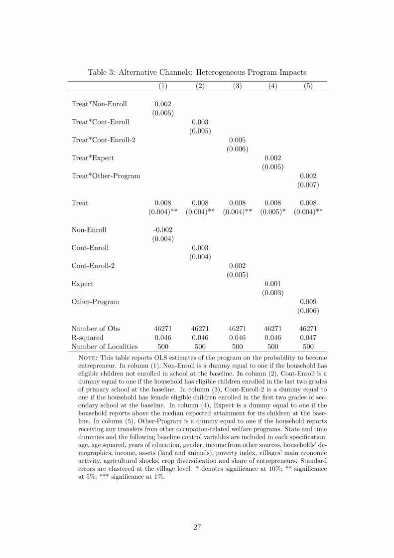
Table 3: Alternative Channels: Heterogeneous Program Impacts
(1) (2) (3) (4) (5)
Treat*Non-Enroll 0.002(0.005)
Treat*Cont-Enroll 0.003(0.005)
Treat*Cont-Enroll-2 0.005(0.006)
Treat*Expect 0.002(0.005)
Treat*Other-Program 0.002(0.007)
Treat 0.008 0.008 0.008 0.008 0.008(0.004)** (0.004)** (0.004)** (0.005)* (0.004)**
Non-Enroll -0.002(0.004)
Cont-Enroll 0.003(0.004)
Cont-Enroll-2 0.002(0.005)
Expect 0.001(0.003)
Other-Program 0.009(0.006)
Number of Obs 46271 46271 46271 46271 46271R-squared 0.046 0.046 0.046 0.046 0.047Number of Localities 500 500 500 500 500
Note: This table reports OLS estimates of the program on the probability to becomeentrepreneur. In column (1), Non-Enroll is a dummy equal to one if the household haseligible children not enrolled in school at the baseline. In column (2), Cont-Enroll is adummy equal to one if the household has eligible children enrolled in the last two gradesof primary school at the baseline. In column (3), Cont-Enroll-2 is a dummy equal toone if the household has female eligible children enrolled in the first two grades of sec-ondary school at the baseline. In column (4), Expect is a dummy equal to one if thehousehold reports above the median expected attainment for its children at the base-line. In column (5), Other-Program is a dummy equal to one if the household reportsreceiving any transfers from other occupation-related welfare programs. State and timedummies and the following baseline control variables are included in each specification:age, age squared, years of education, gender, income from other sources, households’ de-mographics, income, assets (land and animals), poverty index, villages’ main economicactivity, agricultural shocks, crop diversification and share of entrepreneurs. Standarderrors are clustered at the village level. * denotes significance at 10%; ** significanceat 5%; *** significance at 1%.
27
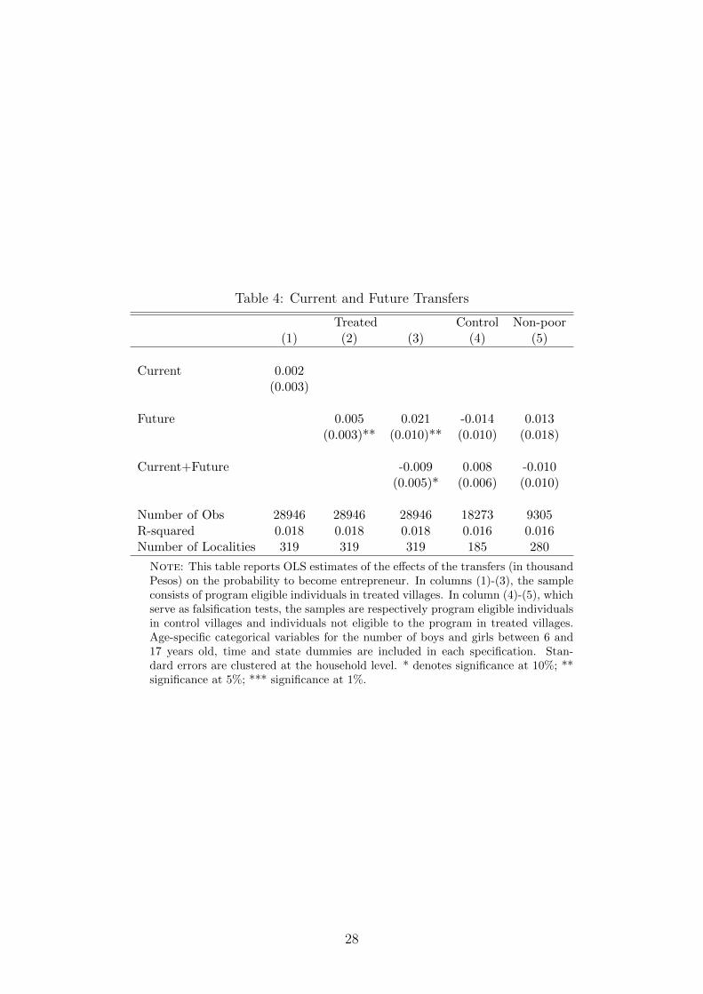
Table 4: Current and Future Transfers
Treated Control Non-poor(1) (2) (3) (4) (5)
Current 0.002(0.003)
Future 0.005 0.021 -0.014 0.013(0.003)** (0.010)** (0.010) (0.018)
Current+Future -0.009 0.008 -0.010(0.005)* (0.006) (0.010)
Number of Obs 28946 28946 28946 18273 9305R-squared 0.018 0.018 0.018 0.016 0.016Number of Localities 319 319 319 185 280
Note: This table reports OLS estimates of the effects of the transfers (in thousandPesos) on the probability to become entrepreneur. In columns (1)-(3), the sampleconsists of program eligible individuals in treated villages. In column (4)-(5), whichserve as falsification tests, the samples are respectively program eligible individualsin control villages and individuals not eligible to the program in treated villages.Age-specific categorical variables for the number of boys and girls between 6 and17 years old, time and state dummies are included in each specification. Stan-dard errors are clustered at the household level. * denotes significance at 10%; **significance at 5%; *** significance at 1%.
28

Table 5: Further Evidence
(1) (2) (3) (4) (5)
Future (6 months) 0.021(0.010)**
Current+Future (6 months) -0.009(0.006)
Total 0.001(0.003)
Future (12 months) 0.002 0.007(0.001)* (0.005)
Current+Future (12 months) -0.002(0.003)
Treat*Risk(village) 0.009(0.004)**
Risk(village) -0.009(0.004)**
Treat*Risk(10km) 0.015(0.005)***
Risk(10km) -0.016(0.005)***
Treat 0.001 -0.011(0.007) (0.008)
Number of Obs 28946 28946 28946 39380 44308R-squared 0.018 0.018 0.018 0.047 0.048Number of Localities 319 319 319 396 472
Note: In columns (1)-(3), we report OLS estimates of the effects of the transfers on the prob-ability to become entrepreneur. Amounts are expressed in thousand Pesos. Control variablesinclude: age-specific categorical variables for the number of boys and girls between 6 and17 years old, time and state dummies. Standard errors are clustered at the household level.In columns (4)-(5), we report OLS estimates of the impact of program on the probability tobecome entrepreneur. The variable Risk(village) is defined as the ratio of the variance of laborincome for the entrepreneurs vs. salaried workers at the village level, based on pre-programincome statements. Risk(10km) is the corresponding variable based on incomes within 10kilometers from each village. Control variables include: age, age squared, years of educa-tion, gender, income from other sources, households’ demographics, income, assets (land andanimals), poverty index, villages’ main economic activity, agricultural shocks, crop diversifi-cation and share of entrepreneurs, time and state dummies. Standard errors are clustered atthe village level. * denotes significance at 10%; ** significance at 5%; *** significance at 1%.
29

Table 6: Medium-term Program Impacts
All High Entrep 97 Low Entrep 97 High Entrep 97 Low Entrep 97(1) (2) (3) (4) (5)
Treat*Post -0.004 -0.031 0.016 -0.019 0.022(0.008) (0.012)** (0.006)*** (0.017) (0.011)**
Treat -0.017 -0.001 -0.011(0.010)* (0.015) (0.004)***
Post 0.0001 -0.010 0.017(0.005) (0.008) (0.004)***
Number of Obs 1300 654 646 8799 8339Number of Localities 650 327 323 327 323R-squared 0.08 0.12 0.15Median % Bias 4.29 4.25P (Treat|X) 0.03 0.02
Note: In columns (1)-(3), we report Weighted Least Squares estimates of the program on the village shareof entrepreneurs in 2003, with analytic weights based on village population size. In column (2), the sample isrestricted to localities with above median share of entrepreneurs in 1997. In column (3), the sample is restrictedto localities with below median share of entrepreneurs in 1997. State dummies are included and standard errorsare clustered at the village level. In columns (4)-(5), we report local linear matching estimates (bandwidth=0.8)of the program on the individual probability to be entrepreneur in 2003. The estimator imposes common support(trimming=2%), and standard errors are computed using bootstrapping with 300 replications. Median % Biasis the median absolute standardized bias after matching and P (Treat|X) is the Pseudo R-squared from a Probitof Treat on all the regressors in the matched sample. * Denotes significance at 10%; ** significance at 5%; ***significance at 1%.
30


![Occupational Choices: Economic Determinants of …tuvalu.santafe.edu/~snaidu/papers/Land_Reform_02sep08.pdfillegal drug trade. Deininger [2003] also finds some support for this latter](https://img.pdfslide.us/doc/110x75/5fb7386e53f64673516bdf8b/occupational-choices-economic-determinants-of-snaidupaperslandreform02sep08pdf.jpg)