Liquid Nitrogen Zero Boiloff Testing

David PlachtaGlenn Research Center, Cleveland, Ohio

Jeffrey FellerAmes Research Center, Moffett Field, California

Wesley Johnson and Craig RobinsonGlenn Research Center, Cleveland, Ohio

Liquid Nitrogen Zero Boiloff Testing

NASA/TP—2017-219389

February 2017

NASA STI Program . . . in Profile

Since its founding, NASA has been dedicated to the advancement of aeronautics and space science. The NASA Scientific and Technical Information (STI) Program plays a key part in helping NASA maintain this important role.

The NASA STI Program operates under the auspices of the Agency Chief Information Officer. It collects, organizes, provides for archiving, and disseminates NASA’s STI. The NASA STI Program provides access to the NASA Technical Report Server—Registered (NTRS Reg) and NASA Technical Report Server—Public (NTRS) thus providing one of the largest collections of aeronautical and space science STI in the world. Results are published in both non-NASA channels and by NASA in the NASA STI Report Series, which includes the following report types: • TECHNICAL PUBLICATION. Reports of

completed research or a major significant phase of research that present the results of NASA programs and include extensive data or theoretical analysis. Includes compilations of significant scientific and technical data and information deemed to be of continuing reference value. NASA counter-part of peer-reviewed formal professional papers, but has less stringent limitations on manuscript length and extent of graphic presentations.

• TECHNICAL MEMORANDUM. Scientific

and technical findings that are preliminary or of specialized interest, e.g., “quick-release” reports, working papers, and bibliographies that contain minimal annotation. Does not contain extensive analysis.

• CONTRACTOR REPORT. Scientific and technical findings by NASA-sponsored contractors and grantees.

• CONFERENCE PUBLICATION. Collected papers from scientific and technical conferences, symposia, seminars, or other meetings sponsored or co-sponsored by NASA.

• SPECIAL PUBLICATION. Scientific,

technical, or historical information from NASA programs, projects, and missions, often concerned with subjects having substantial public interest.

• TECHNICAL TRANSLATION. English-

language translations of foreign scientific and technical material pertinent to NASA’s mission.

For more information about the NASA STI program, see the following:

• Access the NASA STI program home page at http://www.sti.nasa.gov

• E-mail your question to [email protected] • Fax your question to the NASA STI

Information Desk at 757-864-6500

• Telephone the NASA STI Information Desk at 757-864-9658 • Write to:

NASA STI Program Mail Stop 148 NASA Langley Research Center Hampton, VA 23681-2199

http://www.sti.nasa.gov

mailto:help%40sti.nasa.gov?subject=STI%20assistance

David PlachtaGlenn Research Center, Cleveland, Ohio

Jeffrey FellerAmes Research Center, Moffett Field, California

Wesley Johnson and Craig RobinsonGlenn Research Center, Cleveland, Ohio


NASA/TP—2017-219389

February 2017

National Aeronautics andSpace Administration

Glenn Research Center Cleveland, Ohio 44135

Acknowledgments

The authors acknowledge the outstanding cryocooler integration design by Bob Christie of NASA Glenn Research Center (retired) and by Sierra Lobo, Inc.; the design and installation of the multilayer insulation also by Sierra Lobo, Inc.; and the excellent facility engineering support by Helmut Bamberger of Jacob’s Engineering and Tim Czaruk of Glenn. In addition, the authors thank the Cryogenic Propellant Storage and Transfer Program and the Evolvable Cryogenics Program for their support. Both programs are elements of NASA’s Space Technology Mission Directorate.

Available from

Trade names and trademarks are used in this report for identification only. Their usage does not constitute an official endorsement, either expressed or implied, by the National Aeronautics and

Space Administration.

Level of Review: This material has been technically reviewed by expert reviewer(s).

This report contains preliminary findings, subject to revision as analysis proceeds.

NASA STI ProgramMail Stop 148NASA Langley Research CenterHampton, VA 23681-2199

National Technical Information Service5285 Port Royal RoadSpringfield, VA 22161

703-605-6000

This report is available in electronic form at http://www.sti.nasa.gov/ and http://ntrs.nasa.gov/

http://ntrs.nasa.gov/

http://www.sti.nasa.gov/

NASA/TP—2017-219389 iii

Contents 1.0 Executive Summary .............................................................................................................................................. 1 2.0 Background ........................................................................................................................................................... 1

2.1 Cryogenic Boiloff Reduction System Trade Study ..................................................................................... 3 2.2 Scaling Study ............................................................................................................................................... 4 2.3 Trade and Scaling Study Conclusions ......................................................................................................... 5 2.4 Nitrogen as a Surrogate Fluid for Oxygen ................................................................................................... 5

3.0 Objectives ............................................................................................................................................................. 5 4.0 Test Hardware and Instrumentation ...................................................................................................................... 6

4.1 Facility Overview ........................................................................................................................................ 6 4.1.1 Vacuum Chamber ........................................................................................................................... 7 4.1.2 Cryoshroud ...................................................................................................................................... 7 4.1.3 Operations—Fill, Vent, and Pressurization ..................................................................................... 8

4.2 Test Assembly ............................................................................................................................................. 8 4.2.1 Liquid Nitrogen Test Tank .............................................................................................................. 9 4.2.2 Support Ring ................................................................................................................................. 10 4.2.3 Radiator ......................................................................................................................................... 10 4.2.4 Insulation....................................................................................................................................... 11 4.2.5 Broad-Area Cooling ...................................................................................................................... 11 4.2.6 Cryocooler..................................................................................................................................... 12 4.2.7 Cryocooler Data ............................................................................................................................ 13 4.2.8 Test Tank and Facility ................................................................................................................... 14

4.3 Test Plan .................................................................................................................................................... 16 4.3.1 Steady-State Criteria ..................................................................................................................... 17 4.3.2 Pressurization Criteria ................................................................................................................... 17 4.3.3 Test Matrix .................................................................................................................................... 17

5.0 Calculation of Heat Loads .................................................................................................................................. 18 5.1 Propellant Tank Heat ................................................................................................................................. 18

5.1.1 Fluid Heat...................................................................................................................................... 18 5.1.2 Tank Wall Heat ............................................................................................................................. 19

5.2 MLI Heat Leak .......................................................................................................................................... 20 5.3 Cooling Loop Heat Loads .......................................................................................................................... 21 5.4 Error Analysis ............................................................................................................................................ 21

6.0 Test Matrix Summary ......................................................................................................................................... 22 6.1 Test 1: Passive Boiloff ............................................................................................................................... 22 6.2 Test 2. Passive Pressurization .................................................................................................................... 23 6.3 Test 3: Active Zero Boiloff........................................................................................................................ 24 6.4 Test 4: Active High Power A ..................................................................................................................... 24 6.5 Test 5: Active Low Power ......................................................................................................................... 25 6.6 Test 6: Active Destratification ................................................................................................................... 25 6.7 Test 7: Active High Power B ..................................................................................................................... 25 6.8 Test 8: Active Low Fill, Zero Boiloff ........................................................................................................ 26 6.9 Test 9: Active Low Fill, High Power ......................................................................................................... 27 6.10 Test 10: Passive Boiloff at 300 K .............................................................................................................. 27 6.11 Summary of Tests ...................................................................................................................................... 28

7.0 Analysis of Performance ..................................................................................................................................... 28 7.1 Direct Calculation of Heat Loads .............................................................................................................. 28 7.2 Refined Calculation of Heat Loads on the Distributed Cooling Network ................................................. 30

7.2.1 Discussion of Cooling Loop Temperatures and Heat Loads ......................................................... 30 7.2.2 Linearized Cooling Loop Heat Loads ........................................................................................... 31 7.2.3 Parasitic Heat Leaks ...................................................................................................................... 32

7.3 Cryocooler Performance ............................................................................................................................ 33

NASA/TP—2017-219389 iv

7.3.1 Definition of Cryocooler Coefficient of Performance................................................................... 33 7.3.2 Comparison With Creare Bench Test Performance Data .............................................................. 33 7.3.3 Parasitics and Useful Refrigeration ............................................................................................... 34 7.3.4 System Coefficient of Performance .............................................................................................. 34

7.4 Heat Exchanger Thermal Effectiveness ..................................................................................................... 35 7.4.1 Analytical Approach ..................................................................................................................... 35 7.4.2 Cooling Loop Temperature Profiles .............................................................................................. 35 7.4.3 Thermal Conductance and Effectiveness of Tube-on-Tank Heat Exchangers .............................. 36 7.4.4 Dependence of Cryocooler Input Power on Effectiveness ............................................................ 37

7.5 Pressurization Test Analysis ...................................................................................................................... 38 7.5.1 Pressurization Model Comparison to Test Data ............................................................................ 39 7.5.2 Correlation to Liquid Oxygen ....................................................................................................... 39

7.6 Posttest Destructive Analysis .................................................................................................................... 39 7.6.1 Destructive Investigation .............................................................................................................. 40 7.6.2 Analysis of Cryocooler Integration Losses ................................................................................... 41 7.6.3 Improved Cryocooler Integration Design and Analysis ................................................................ 44

7.7 Multilayer Insulation ................................................................................................................................. 44 7.7.1 Multilayer Insulation Analysis ...................................................................................................... 44 7.7.2 Multilayer Insulation Temperature Gradients ............................................................................... 46

7.8 Radiator Performance ................................................................................................................................ 47 8.0 Discussion of Results .......................................................................................................................................... 47

8.1 Component Performance ........................................................................................................................... 47 8.1.1 Broad-Area Cooling Loop/Heat Exchanger .................................................................................. 48 8.1.2 Cryocooler..................................................................................................................................... 48 8.1.3 Parasitic Loss ................................................................................................................................ 48 8.1.4 Radiator ......................................................................................................................................... 49 8.1.5 MLI ............................................................................................................................................... 49

8.2 Revisiting Test Objectives ......................................................................................................................... 49 8.2.1 Robust Tank Pressure Control ...................................................................................................... 49 8.2.2 ZBO at Low Fill Level .................................................................................................................. 49 8.2.3 Validation of Scaling Study .......................................................................................................... 50 8.2.4 MLI Database ................................................................................................................................ 50

9.0 Liquid Nitrogen Zero Boiloff Test Conclusions ................................................................................................. 50 Appendix A.—Symbols ............................................................................................................................................... 53 Appendix B.—Instrumentation .................................................................................................................................... 55 References ................................................................................................................................................................... 65

NASA/TP—2017-219389 1


David Plachta National Aeronautics and Space Administration


Jeffrey Feller

National Aeronautics and Space Administration Ames Research Center

Moffett Field, California 94035

Wesley Johnson and Craig Robinson National Aeronautics and Space Administration


1.0 Executive Summary NASA is working in earnest to improve the utilization of

high-specific-impulse propellant combinations such as liquid hydrogen and oxygen (LH2 and LO2). These efforts are prerequisite to achieving a human presence on the surface of Mars and to facilitating an expanded presence across the solar system. Realization of these goals underlies the need to store and manage high-energy propellants for extended periods of time, and under conditions of microgravity. NASA therefore continues to devote considerable human and capital resources to the development of orbiting depots, orbit transfer stages, and related technologies.

Volumetric considerations require that hydrogen and oxygen propellants be stored as liquids at extremely low temperatures. This constitutes a formidable engineering challenge in light of anticipated natural environments in space. Heat radiated to a spacecraft from the Sun and other celestial bodies in proximity to the spacecraft (such as Earth, the Moon, and Mars), in addition to heat conducted to the storage tanks from other sources on the spacecraft, cause LH2 and LO2 to pressurize and boil off (i.e., change state from liquid to gas). In the absence of effective thermal protection and control measures, the storage tanks will overpressurize; hence, a portion of the vaporized liquid must be released (or “vented”) to preserve the structural integrity of the tanks. Venting results in less propellant available for propulsion. Because mission loiter periods are projected to be months long, vented losses will be substantial. To offset these losses, the stage would need to accommodate excess propellant, thus substantially increasing the mass of the stage. Alternatively, NASA could use thick-walled propellant tanks in conjunction with greater working pressures, but the additional mass of the tanks would be prohibitive.

Application of zero boiloff (ZBO) technology to prevent vaporization, while maintaining tanks of reasonable size and weight, will ensure adequate propellant quantities for extended periods of time. Development work on this concept has been ongoing at NASA since 1998 and has continued with a focus on distributed cooling with the Cryogenic Boil-Off Reduction System activities. Analysis results pertinent to the ZBO concept, as applied to LO2 tanks, suggest that implementation of ZBO technologies will reduce mass for missions in low Earth orbit having loiter periods greater than 1 week. The distributed cooling system utilizes the reverse turbo-Brayton-cycle cryocooler (and the circulator that is inherent to it). This concept and associated technology was demonstrated in a series of 10 tests performed at the NASA Glenn Research Center’s Small Multi-Purpose Research Facility. Three of the aforementioned tests were “passive” (conducted with the cryocooler system off), and the remaining seven tests were “active” (conducted with the cryo-cooler system operational). The series included tests performed for tank fill levels of approximately 90 and 25 percent. Tests were further conducted by adjusting cryocooler input power to increase or decrease pressure. Test results clearly established that the prescribed system, with integrated cryocooler, eliminated boiloff and effectively controlled tank pressure.

2.0 Background During the mid-1990s, various concepts were defined to

achieve zero boiloff (ZBO) propellant storage. Subsequent evaluation and comparison of these concepts began in support of a NASA effort to define a human mission to Mars (Refs. 1 and 2). A number of prospective mission timelines were con-sidered, most requiring in-space loiter periods for cryogenic propellants of up to 1200 days (Refs. 3 and. 4). Results

NASA/TP—2017-219389 2

compiled in the course of these studies showed that refriger-ation of the propellants is paramount to mission success. Moreover, the use of cryocoolers constitutes an enabling technology to this end.

ZBO testing began first at the NASA Glenn Research Center (Ref. 5) in 1998, followed by additional testing at the NASA Marshall Space Flight Center (Ref. 6) in 2001. The common objective was to assess the feasibility of ZBO concepts using readily available components. The first proof of concept incor-porated a cryocooler at the top of a liquid hydrogen (LH2) propellant tank and a copper shield within the multilayer insulation (MLI). This test demonstrated ZBO utilizing 14.5 W of the cryocooler’s 17-W specified capacity for heat removal. A steady decline in tank pressure was measured with the vent valve closed. However, the corresponding 8-K temperature gradient on the heat exchanger was excessive. Given that cryo-cooler performance is a function of the respective cold head temperature, this 8-K gradient requires the cryocooler to oper-ate 8-K colder, causing a significant loss in heat “lift” (or an increase in power). Also, this test was not flightlike because it used fluid buoyancy to convey heat to the cryocooler (which cannot happen in space); an industrial cryocooler was also used. The Marshall test was more flightlike insofar as LH2 was pumped through an actively cooled bypass loop to facilitate heat extraction. ZBO was easily achieved because the industrial

cryocooler lift was 30 W and the tank heat leak was just 8.3 W. However, continuous pump operation added 0.3 W to the fluid while flow through the bypass loop increased the insulation heat leak into the tank. Thermal performance was further reduced by an observed 2-K increase in the temperature of the copper fin that coupled the cryocooler to the bypass loop.

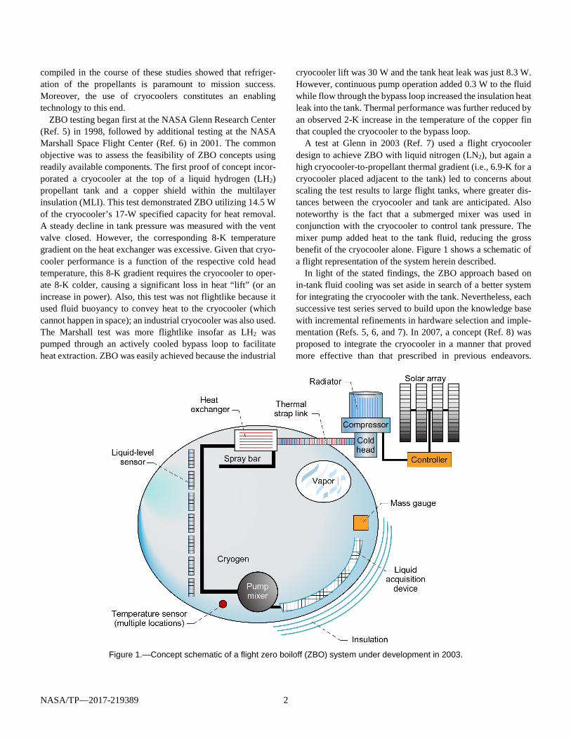
A test at Glenn in 2003 (Ref. 7) used a flight cryocooler design to achieve ZBO with liquid nitrogen (LN2), but again a high cryocooler-to-propellant thermal gradient (i.e., 6.9-K for a cryocooler placed adjacent to the tank) led to concerns about scaling the test results to large flight tanks, where greater dis-tances between the cryocooler and tank are anticipated. Also noteworthy is the fact that a submerged mixer was used in conjunction with the cryocooler to control tank pressure. The mixer pump added heat to the tank fluid, reducing the gross benefit of the cryocooler alone. Figure 1 shows a schematic of a flight representation of the system herein described.

In light of the stated findings, the ZBO approach based on in-tank fluid cooling was set aside in search of a better system for integrating the cryocooler with the tank. Nevertheless, each successive test series served to build upon the knowledge base with incremental refinements in hardware selection and imple-mentation (Refs. 5, 6, and 7). In 2007, a concept (Ref. 8) was proposed to integrate the cryocooler in a manner that proved more effective than that prescribed in previous endeavors.

Figure 1.—Concept schematic of a flight zero boiloff (ZBO) system under development in 2003.

NASA/TP—2017-219389 3

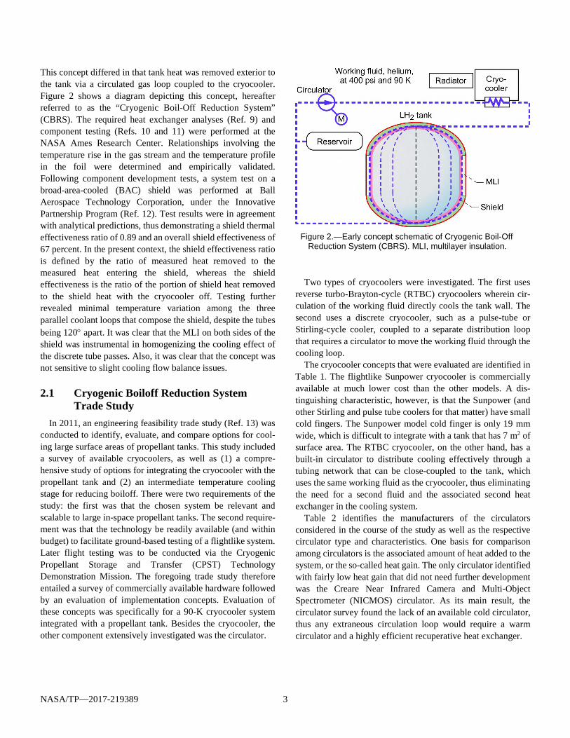
This concept differed in that tank heat was removed exterior to the tank via a circulated gas loop coupled to the cryocooler. Figure 2 shows a diagram depicting this concept, hereafter referred to as the “Cryogenic Boil-Off Reduction System” (CBRS). The required heat exchanger analyses (Ref. 9) and component testing (Refs. 10 and 11) were performed at the NASA Ames Research Center. Relationships involving the temperature rise in the gas stream and the temperature profile in the foil were determined and empirically validated. Following component development tests, a system test on a broad-area-cooled (BAC) shield was performed at Ball Aerospace Technology Corporation, under the Innovative Partnership Program (Ref. 12). Test results were in agreement with analytical predictions, thus demonstrating a shield thermal effectiveness ratio of 0.89 and an overall shield effectiveness of 67 percent. In the present context, the shield effectiveness ratio is defined by the ratio of measured heat removed to the measured heat entering the shield, whereas the shield effectiveness is the ratio of the portion of shield heat removed to the shield heat with the cryocooler off. Testing further revealed minimal temperature variation among the three parallel coolant loops that compose the shield, despite the tubes being 120° apart. It was clear that the MLI on both sides of the shield was instrumental in homogenizing the cooling effect of the discrete tube passes. Also, it was clear that the concept was not sensitive to slight cooling flow balance issues.

2.1 Cryogenic Boiloff Reduction System Trade Study

In 2011, an engineering feasibility trade study (Ref. 13) was conducted to identify, evaluate, and compare options for cool-ing large surface areas of propellant tanks. This study included a survey of available cryocoolers, as well as (1) a compre-hensive study of options for integrating the cryocooler with the propellant tank and (2) an intermediate temperature cooling stage for reducing boiloff. There were two requirements of the study: the first was that the chosen system be relevant and scalable to large in-space propellant tanks. The second require-ment was that the technology be readily available (and within budget) to facilitate ground-based testing of a flightlike system. Later flight testing was to be conducted via the Cryogenic Propellant Storage and Transfer (CPST) Technology Demonstration Mission. The foregoing trade study therefore entailed a survey of commercially available hardware followed by an evaluation of implementation concepts. Evaluation of these concepts was specifically for a 90-K cryocooler system integrated with a propellant tank. Besides the cryocooler, the other component extensively investigated was the circulator.

Figure 2.—Early concept schematic of Cryogenic Boil-Off

Reduction System (CBRS). MLI, multilayer insulation.

Two types of cryocoolers were investigated. The first uses reverse turbo-Brayton-cycle (RTBC) cryocoolers wherein cir-culation of the working fluid directly cools the tank wall. The second uses a discrete cryocooler, such as a pulse-tube or Stirling-cycle cooler, coupled to a separate distribution loop that requires a circulator to move the working fluid through the cooling loop.

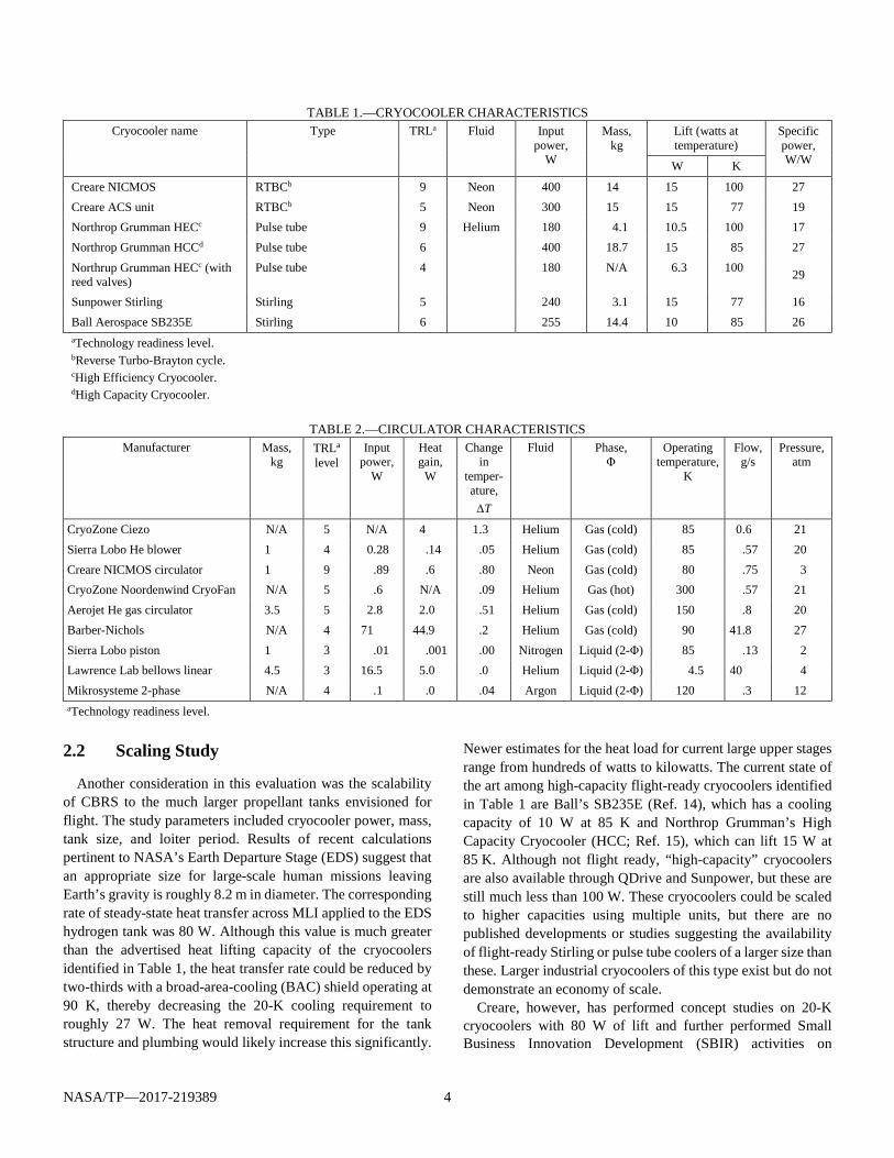
The cryocooler concepts that were evaluated are identified in Table 1. The flightlike Sunpower cryocooler is commercially available at much lower cost than the other models. A dis-tinguishing characteristic, however, is that the Sunpower (and other Stirling and pulse tube coolers for that matter) have small cold fingers. The Sunpower model cold finger is only 19 mm wide, which is difficult to integrate with a tank that has 7 m2 of surface area. The RTBC cryocooler, on the other hand, has a built-in circulator to distribute cooling effectively through a tubing network that can be close-coupled to the tank, which uses the same working fluid as the cryocooler, thus eliminating the need for a second fluid and the associated second heat exchanger in the cooling system.

Table 2 identifies the manufacturers of the circulators considered in the course of the study as well as the respective circulator type and characteristics. One basis for comparison among circulators is the associated amount of heat added to the system, or the so-called heat gain. The only circulator identified with fairly low heat gain that did not need further development was the Creare Near Infrared Camera and Multi-Object Spectrometer (NICMOS) circulator. As its main result, the circulator survey found the lack of an available cold circulator, thus any extraneous circulation loop would require a warm circulator and a highly efficient recuperative heat exchanger.

NASA/TP—2017-219389 4

TABLE 1.—CRYOCOOLER CHARACTERISTICS Cryocooler name Type TRLa Fluid Input

power, W

Mass, kg

Lift (watts at temperature)

Specific power, W/W W K

Creare NICMOS RTBCb 9 Neon 400 14 15 100 27 Creare ACS unit RTBCb 5 Neon 300 15 15 77 19 Northrop Grumman HECc Pulse tube 9 Helium 180 4.1 10.5 100 17 Northrop Grumman HCCd Pulse tube 6 400 18.7 15 85 27 Northrup Grumman HECc (with reed valves)

Pulse tube 4 180 N/A 6.3 100 29

Sunpower Stirling Stirling 5 240 3.1 15 77 16 Ball Aerospace SB235E Stirling 6 255 14.4 10 85 26 aTechnology readiness level. bReverse Turbo-Brayton cycle. cHigh Efficiency Cryocooler. dHigh Capacity Cryocooler.

TABLE 2.—CIRCULATOR CHARACTERISTICS

Manufacturer Mass, kg

TRLa

level Input

power, W

Heat gain,

W

Change in

temper-ature,

∆T

Fluid Phase, Φ

Operating temperature,

K

Flow, g/s

Pressure, atm

CryoZone Ciezo N/A 5 N/A 4 1.3 Helium Gas (cold) 85 0.6 21 Sierra Lobo He blower 1 4 0.28 .14 .05 Helium Gas (cold) 85 .57 20 Creare NICMOS circulator 1 9 .89 .6 .80 Neon Gas (cold) 80 .75 3 CryoZone Noordenwind CryoFan N/A 5 .6 N/A .09 Helium Gas (hot) 300 .57 21 Aerojet He gas circulator 3.5 5 2.8 2.0 .51 Helium Gas (cold) 150 .8 20 Barber-Nichols N/A 4 71 44.9 .2 Helium Gas (cold) 90 41.8 27 Sierra Lobo piston 1 3 .01 .001 .00 Nitrogen Liquid (2-Φ) 85 .13 2 Lawrence Lab bellows linear 4.5 3 16.5 5.0 .0 Helium Liquid (2-Φ) 4.5 40 4 Mikrosysteme 2-phase N/A 4 .1 .0 .04 Argon Liquid (2-Φ) 120 .3 12 aTechnology readiness level.

2.2 Scaling Study

Another consideration in this evaluation was the scalability of CBRS to the much larger propellant tanks envisioned for flight. The study parameters included cryocooler power, mass, tank size, and loiter period. Results of recent calculations pertinent to NASA’s Earth Departure Stage (EDS) suggest that an appropriate size for large-scale human missions leaving Earth’s gravity is roughly 8.2 m in diameter. The corresponding rate of steady-state heat transfer across MLI applied to the EDS hydrogen tank was 80 W. Although this value is much greater than the advertised heat lifting capacity of the cryocoolers identified in Table 1, the heat transfer rate could be reduced by two-thirds with a broad-area-cooling (BAC) shield operating at 90 K, thereby decreasing the 20-K cooling requirement to roughly 27 W. The heat removal requirement for the tank structure and plumbing would likely increase this significantly.

Newer estimates for the heat load for current large upper stages range from hundreds of watts to kilowatts. The current state of the art among high-capacity flight-ready cryocoolers identified in Table 1 are Ball’s SB235E (Ref. 14), which has a cooling capacity of 10 W at 85 K and Northrop Grumman’s High Capacity Cryocooler (HCC; Ref. 15), which can lift 15 W at 85 K. Although not flight ready, “high-capacity” cryocoolers are also available through QDrive and Sunpower, but these are still much less than 100 W. These cryocoolers could be scaled to higher capacities using multiple units, but there are no published developments or studies suggesting the availability of flight-ready Stirling or pulse tube coolers of a larger size than these. Larger industrial cryocoolers of this type exist but do not demonstrate an economy of scale.

Creare, however, has performed concept studies on 20-K cryocoolers with 80 W of lift and further performed Small Business Innovation Development (SBIR) activities on

NASA/TP—2017-219389 5

cryocoolers with over 1000 W of lift (Refs. 16 and 17). Creare notes (Ref. 17) that the specific mass, defined as the system mass per unit of heat lift (kilograms per watt), could be halved using very large cryocoolers. Their RTBC scaling study, done for more reasonably sized cryocoolers, shows the specific mass and power to be inversely proportional to cryocooler size and capacity. Table 3 and Table 4 illustrate this general trend.

2.3 Trade and Scaling Study Conclusions Results of the trade and scaling studies suggest that the RTBC

cryocooler/circulator is well suited for extended-duration cryogenic propellant storage. Significant characteristics of this technology are that it scales well to large tank sizes and that a state-of-the-art model was available for procurement, with slight modification. The other important aspect to this operating cycle is that it functions as both the circulator and the cryocooler. This eliminates a separate circulator and the heat exchanger that would have been required between the circulator and the cryocooler, thus simplifying integration with the propellant tank and improving system efficiency. Hence, the cryocooler system selected for this test series was the RTBC cryocooler.

2.4 Nitrogen as a Surrogate Fluid for Oxygen Ground testing was planned to demonstrate the extent to

which liquid oxygen (LO2) ZBO could be achieved for the CPST technology demonstrator. Ground test data (in con-junction with flight data from storing LH2 in space) are necessary such that predicative performance models can be used to design and analyze long-duration propellant storage systems. Although CPST was interested in LO2 ZBO data, LN2 was used as a simulant cryogenic fluid because it is safer, easier to work with, and does not require precision cleaning. Thus, using LN2 saved money and reduced schedule while alleviating safety issues with the test.

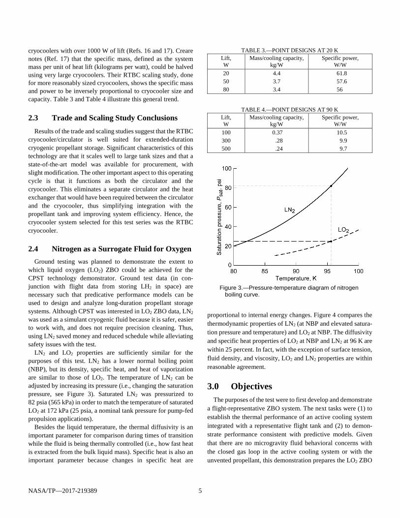
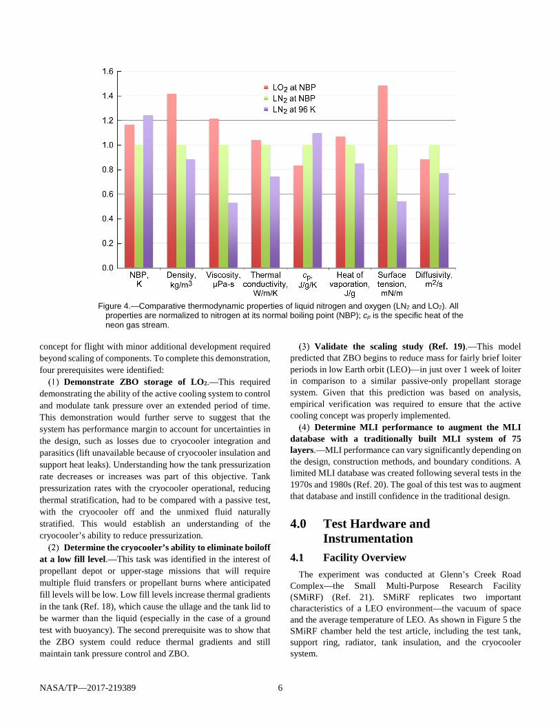
LN2 and LO2 properties are sufficiently similar for the purposes of this test. LN2 has a lower normal boiling point (NBP), but its density, specific heat, and heat of vaporization are similar to those of LO2. The temperature of LN2 can be adjusted by increasing its pressure (i.e., changing the saturation pressure, see Figure 3). Saturated LN2 was pressurized to 82 psia (565 kPa) in order to match the temperature of saturated LO2 at 172 kPa (25 psia, a nominal tank pressure for pump-fed propulsion applications).

Besides the liquid temperature, the thermal diffusivity is an important parameter for comparison during times of transition while the fluid is being thermally controlled (i.e., how fast heat is extracted from the bulk liquid mass). Specific heat is also an important parameter because changes in specific heat are

TABLE 3.—POINT DESIGNS AT 20 K Lift, W

Mass/cooling capacity, kg/W

Specific power, W/W

20 4.4 61.8 50 3.7 57.6 80 3.4 56

TABLE 4.—POINT DESIGNS AT 90 K

Lift, W

Mass/cooling capacity, kg/W

Specific power, W/W

100 0.37 10.5 300 .28 9.9 500 .24 9.7

Figure 3.—Pressure-temperature diagram of nitrogen

boiling curve.

proportional to internal energy changes. Figure 4 compares the thermodynamic properties of LN2 (at NBP and elevated satura-tion pressure and temperature) and LO2 at NBP. The diffusivity and specific heat properties of LO2 at NBP and LN2 at 96 K are within 25 percent. In fact, with the exception of surface tension, fluid density, and viscosity, LO2 and LN2 properties are within reasonable agreement.

3.0 Objectives The purposes of the test were to first develop and demonstrate

a flight-representative ZBO system. The next tasks were (1) to establish the thermal performance of an active cooling system integrated with a representative flight tank and (2) to demon-strate performance consistent with predictive models. Given that there are no microgravity fluid behavioral concerns with the closed gas loop in the active cooling system or with the unvented propellant, this demonstration prepares the LO2 ZBO

NASA/TP—2017-219389 6

Figure 4.—Comparative thermodynamic properties of liquid nitrogen and oxygen (LN2 and LO2). All

properties are normalized to nitrogen at its normal boiling point (NBP); cp is the specific heat of the neon gas stream.

concept for flight with minor additional development required beyond scaling of components. To complete this demonstration, four prerequisites were identified:

Demonstrate ZBO storage of LO2.—This required demonstrating the ability of the active cooling system to control and modulate tank pressure over an extended period of time. This demonstration would further serve to suggest that the system has performance margin to account for uncertainties in the design, such as losses due to cryocooler integration and parasitics (lift unavailable because of cryocooler insulation and support heat leaks). Understanding how the tank pressurization rate decreases or increases was part of this objective. Tank pressurization rates with the cryocooler operational, reducing thermal stratification, had to be compared with a passive test, with the cryocooler off and the unmixed fluid naturally stratified. This would establish an understanding of the cryocooler’s ability to reduce pressurization.

Determine the cryocooler’s ability to eliminate boiloff at a low fill level.—This task was identified in the interest of propellant depot or upper-stage missions that will require multiple fluid transfers or propellant burns where anticipated fill levels will be low. Low fill levels increase thermal gradients in the tank (Ref. 18), which cause the ullage and the tank lid to be warmer than the liquid (especially in the case of a ground test with buoyancy). The second prerequisite was to show that the ZBO system could reduce thermal gradients and still maintain tank pressure control and ZBO.

Validate the scaling study (Ref. 19).—This model predicted that ZBO begins to reduce mass for fairly brief loiter periods in low Earth orbit (LEO)—in just over 1 week of loiter in comparison to a similar passive-only propellant storage system. Given that this prediction was based on analysis, empirical verification was required to ensure that the active cooling concept was properly implemented.

Determine MLI performance to augment the MLI database with a traditionally built MLI system of 75 layers.—MLI performance can vary significantly depending on the design, construction methods, and boundary conditions. A limited MLI database was created following several tests in the 1970s and 1980s (Ref. 20). The goal of this test was to augment that database and instill confidence in the traditional design.

4.0 Test Hardware and Instrumentation

4.1 Facility Overview The experiment was conducted at Glenn’s Creek Road

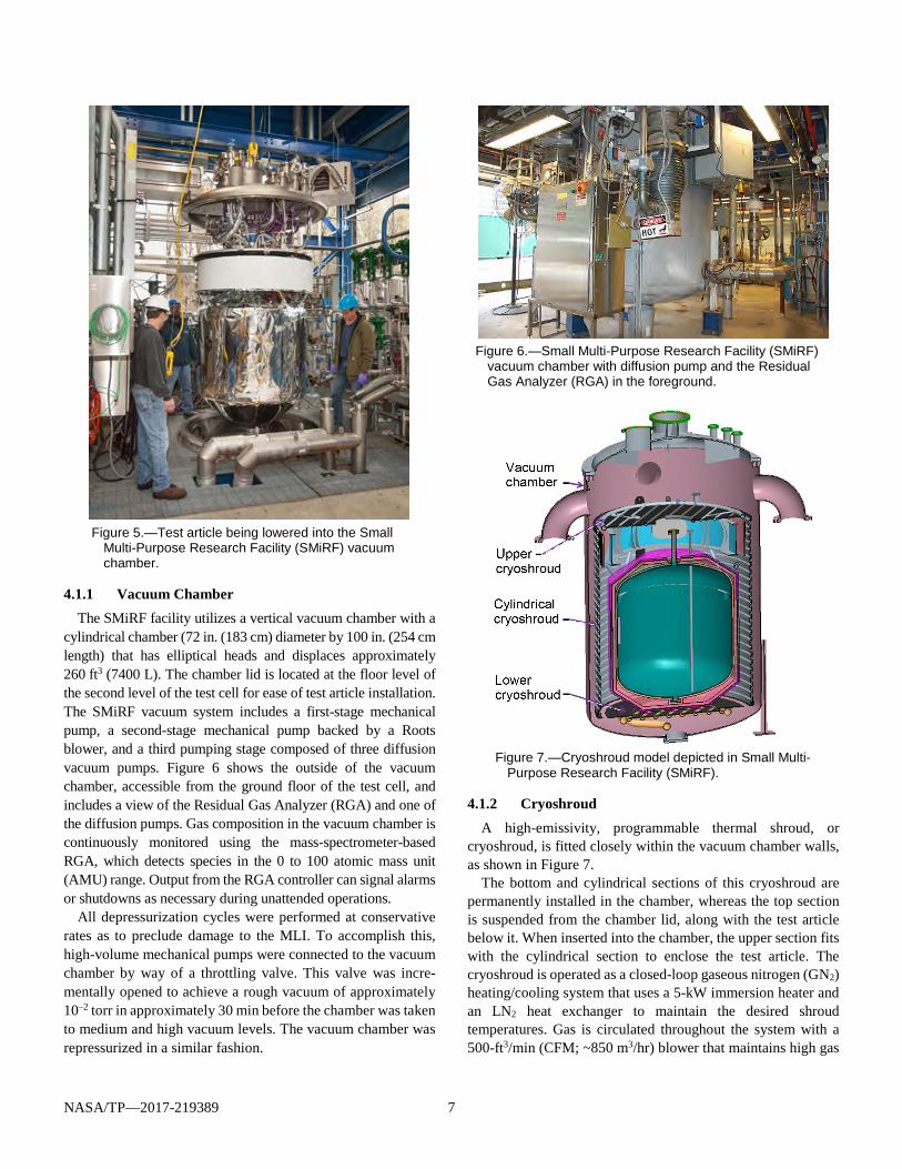
Complex—the Small Multi-Purpose Research Facility (SMiRF) (Ref. 21). SMiRF replicates two important characteristics of a LEO environment—the vacuum of space and the average temperature of LEO. As shown in Figure 5 the SMiRF chamber held the test article, including the test tank, support ring, radiator, tank insulation, and the cryocooler system.

NASA/TP—2017-219389 7

Figure 5.—Test article being lowered into the Small

Multi-Purpose Research Facility (SMiRF) vacuum chamber.

4.1.1 Vacuum Chamber The SMiRF facility utilizes a vertical vacuum chamber with a

cylindrical chamber (72 in. (183 cm) diameter by 100 in. (254 cm length) that has elliptical heads and displaces approximately 260 ft3 (7400 L). The chamber lid is located at the floor level of the second level of the test cell for ease of test article installation. The SMiRF vacuum system includes a first-stage mechanical pump, a second-stage mechanical pump backed by a Roots blower, and a third pumping stage composed of three diffusion vacuum pumps. Figure 6 shows the outside of the vacuum chamber, accessible from the ground floor of the test cell, and includes a view of the Residual Gas Analyzer (RGA) and one of the diffusion pumps. Gas composition in the vacuum chamber is continuously monitored using the mass-spectrometer-based RGA, which detects species in the 0 to 100 atomic mass unit (AMU) range. Output from the RGA controller can signal alarms or shutdowns as necessary during unattended operations.

All depressurization cycles were performed at conservative rates as to preclude damage to the MLI. To accomplish this, high-volume mechanical pumps were connected to the vacuum chamber by way of a throttling valve. This valve was incre-mentally opened to achieve a rough vacuum of approximately 10–2 torr in approximately 30 min before the chamber was taken to medium and high vacuum levels. The vacuum chamber was repressurized in a similar fashion.

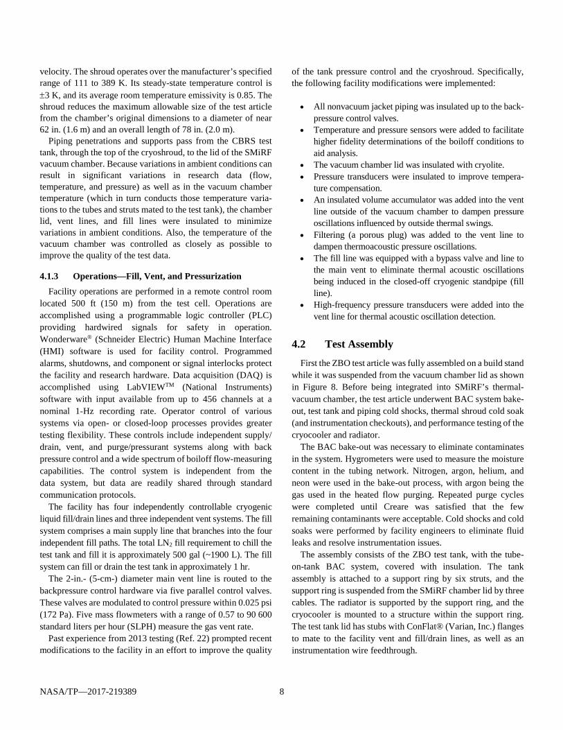
Figure 6.—Small Multi-Purpose Research Facility (SMiRF)

vacuum chamber with diffusion pump and the Residual Gas Analyzer (RGA) in the foreground.

Figure 7.—Cryoshroud model depicted in Small Multi-

Purpose Research Facility (SMiRF).

4.1.2 Cryoshroud A high-emissivity, programmable thermal shroud, or

cryoshroud, is fitted closely within the vacuum chamber walls, as shown in Figure 7.

The bottom and cylindrical sections of this cryoshroud are permanently installed in the chamber, whereas the top section is suspended from the chamber lid, along with the test article below it. When inserted into the chamber, the upper section fits with the cylindrical section to enclose the test article. The cryoshroud is operated as a closed-loop gaseous nitrogen (GN2) heating/cooling system that uses a 5-kW immersion heater and an LN2 heat exchanger to maintain the desired shroud temperatures. Gas is circulated throughout the system with a 500-ft3/min (CFM; ~850 m3/hr) blower that maintains high gas

NASA/TP—2017-219389 8

velocity. The shroud operates over the manufacturer’s specified range of 111 to 389 K. Its steady-state temperature control is ±3 K, and its average room temperature emissivity is 0.85. The shroud reduces the maximum allowable size of the test article from the chamber’s original dimensions to a diameter of near 62 in. (1.6 m) and an overall length of 78 in. (2.0 m).

Piping penetrations and supports pass from the CBRS test tank, through the top of the cryoshroud, to the lid of the SMiRF vacuum chamber. Because variations in ambient conditions can result in significant variations in research data (flow, temperature, and pressure) as well as in the vacuum chamber temperature (which in turn conducts those temperature varia-tions to the tubes and struts mated to the test tank), the chamber lid, vent lines, and fill lines were insulated to minimize variations in ambient conditions. Also, the temperature of the vacuum chamber was controlled as closely as possible to improve the quality of the test data.

4.1.3 Operations—Fill, Vent, and Pressurization Facility operations are performed in a remote control room

located 500 ft (150 m) from the test cell. Operations are accomplished using a programmable logic controller (PLC) providing hardwired signals for safety in operation. Wonderware® (Schneider Electric) Human Machine Interface (HMI) software is used for facility control. Programmed alarms, shutdowns, and component or signal interlocks protect the facility and research hardware. Data acquisition (DAQ) is accomplished using LabVIEWTM (National Instruments) software with input available from up to 456 channels at a nominal 1-Hz recording rate. Operator control of various systems via open- or closed-loop processes provides greater testing flexibility. These controls include independent supply/ drain, vent, and purge/pressurant systems along with back pressure control and a wide spectrum of boiloff flow-measuring capabilities. The control system is independent from the data system, but data are readily shared through standard communication protocols.

The facility has four independently controllable cryogenic liquid fill/drain lines and three independent vent systems. The fill system comprises a main supply line that branches into the four independent fill paths. The total LN2 fill requirement to chill the test tank and fill it is approximately 500 gal (~1900 L). The fill system can fill or drain the test tank in approximately 1 hr.

The 2-in.- (5-cm-) diameter main vent line is routed to the backpressure control hardware via five parallel control valves. These valves are modulated to control pressure within 0.025 psi (172 Pa). Five mass flowmeters with a range of 0.57 to 90 600 standard liters per hour (SLPH) measure the gas vent rate.

Past experience from 2013 testing (Ref. 22) prompted recent modifications to the facility in an effort to improve the quality

of the tank pressure control and the cryoshroud. Specifically, the following facility modifications were implemented:

• All nonvacuum jacket piping was insulated up to the back-

pressure control valves. • Temperature and pressure sensors were added to facilitate

higher fidelity determinations of the boiloff conditions to aid analysis.

• The vacuum chamber lid was insulated with cryolite. • Pressure transducers were insulated to improve tempera-

ture compensation. • An insulated volume accumulator was added into the vent

line outside of the vacuum chamber to dampen pressure oscillations influenced by outside thermal swings.

• Filtering (a porous plug) was added to the vent line to dampen thermoacoustic pressure oscillations.

• The fill line was equipped with a bypass valve and line to the main vent to eliminate thermal acoustic oscillations being induced in the closed-off cryogenic standpipe (fill line).

• High-frequency pressure transducers were added into the vent line for thermal acoustic oscillation detection.

4.2 Test Assembly

First the ZBO test article was fully assembled on a build stand while it was suspended from the vacuum chamber lid as shown in Figure 8. Before being integrated into SMiRF’s thermal-vacuum chamber, the test article underwent BAC system bake-out, test tank and piping cold shocks, thermal shroud cold soak (and instrumentation checkouts), and performance testing of the cryocooler and radiator.

The BAC bake-out was necessary to eliminate contaminates in the system. Hygrometers were used to measure the moisture content in the tubing network. Nitrogen, argon, helium, and neon were used in the bake-out process, with argon being the gas used in the heated flow purging. Repeated purge cycles were completed until Creare was satisfied that the few remaining contaminants were acceptable. Cold shocks and cold soaks were performed by facility engineers to eliminate fluid leaks and resolve instrumentation issues.

The assembly consists of the ZBO test tank, with the tube-on-tank BAC system, covered with insulation. The tank assembly is attached to a support ring by six struts, and the support ring is suspended from the SMiRF chamber lid by three cables. The radiator is supported by the support ring, and the cryocooler is mounted to a structure within the support ring. The test tank lid has stubs with ConFlat® (Varian, Inc.) flanges to mate to the facility vent and fill/drain lines, as well as an instrumentation wire feedthrough.

NASA/TP—2017-219389 9

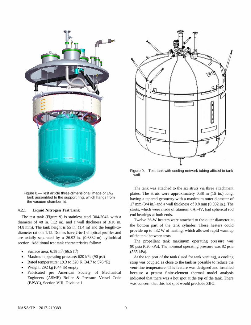
Figure 8.—Test article three-dimensional image of LN2

tank assembled to the support ring, which hangs from the vacuum chamber lid.

4.2.1 Liquid Nitrogen Test Tank The test tank (Figure 9) is stainless steel 304/304L with a

diameter of 48 in. (1.2 m), and a wall thickness of 3/16 in. (4.8 mm). The tank height is 55 in. (1.4 m) and the length-to-diameter ratio is 1.15. Domes have 2-to-1 elliptical profiles and are axially separated by a 26.92-in. (0.6832-m) cylindrical section. Additional test tank characteristics follow:

• Surface area: 6.18 m2 (66.5 ft2) • Maximum operating pressure: 620 kPa (90 psi) • Rated temperature: 19.3 to 320 K (34.7 to 576 °R) • Weight: 292 kg (644 lb) empty • Fabricated per American Society of Mechanical

Engineers (ASME) Boiler & Pressure Vessel Code (BPVC), Section VIII, Division 1

Figure 9.—Test tank with cooling network tubing affixed to tank

wall.

The tank was attached to the six struts via three attachment

plates. The struts were approximately 0.38 m (15 in.) long, having a tapered geometry with a maximum outer diameter of 17 mm (3/4 in.) and a wall thickness of 0.8 mm (0.032 in.). The struts, which were made of titanium 6Al-4V, had spherical rod end bearings at both ends.

Twelve 36-W heaters were attached to the outer diameter at the bottom part of the tank cylinder. These heaters could provide up to 432 W of heating, which allowed rapid warmup of the tank between tests.

The propellant tank maximum operating pressure was 90 psia (620 kPa). The nominal operating pressure was 82 psia (565 kPa).

At the top port of the tank (used for tank venting), a cooling strap was coupled as close to the tank as possible to reduce the vent-line temperature. This feature was designed and installed because a pretest finite-element thermal model analysis indicated that there was a hot spot at the top of the tank. There was concern that this hot spot would preclude ZBO.

NASA/TP—2017-219389 10

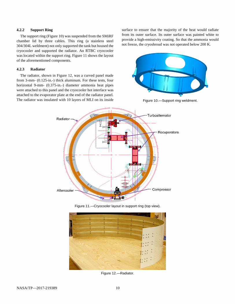
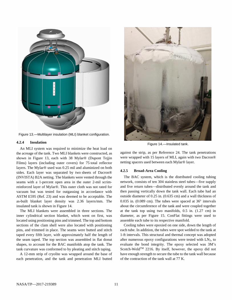
4.2.2 Support Ring The support ring (Figure 10) was suspended from the SMiRF

chamber lid by three cables. This ring (a stainless steel 304/304L weldment) not only supported the tank but housed the cryocooler and supported the radiator. An RTBC cryocooler was located within the support ring. Figure 11 shows the layout of the aforementioned components.

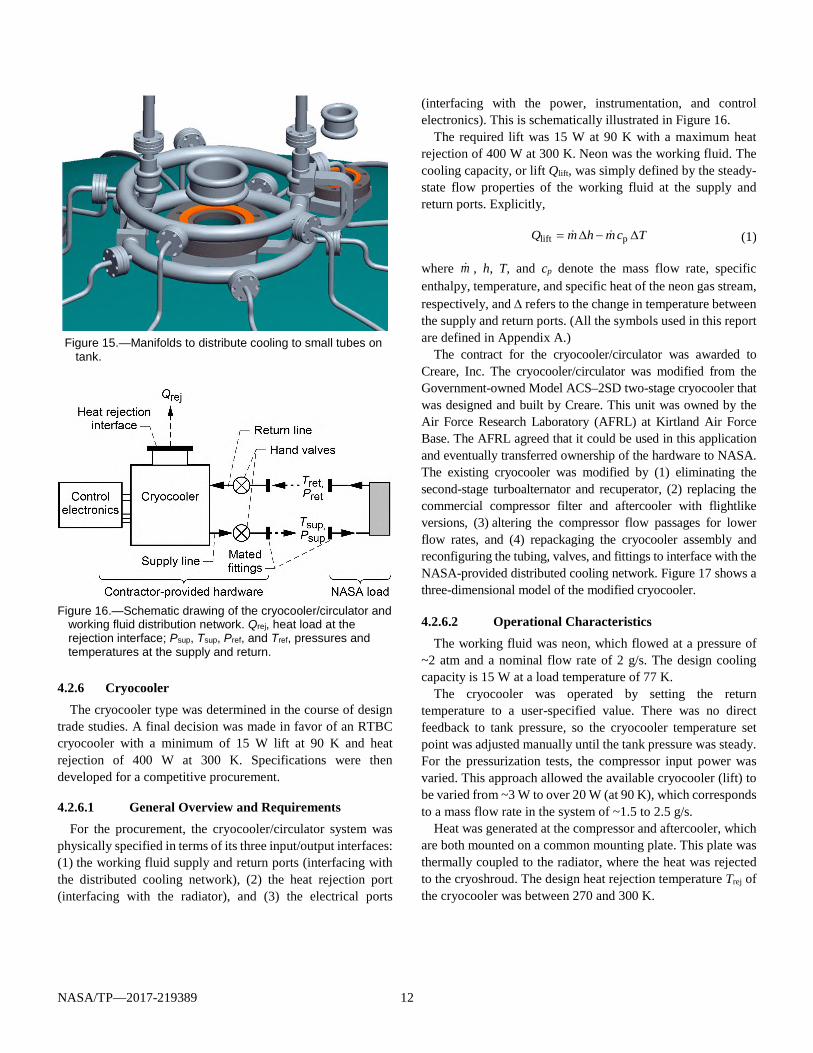
4.2.3 Radiator The radiator, shown in Figure 12, was a curved panel made

from 3-mm- (0.125-in.-) thick aluminum. For these tests, four horizontal 9-mm- (0.375-in.-) diameter ammonia heat pipes were attached to this panel and the cryocooler hot interface was attached to the evaporator plate at the end of the radiator panel. The radiator was insulated with 10 layers of MLI on its inside

surface to ensure that the majority of the heat would radiate from its outer surface. Its outer surface was painted white to provide a high-emissivity coating. So that the ammonia would not freeze, the cryoshroud was not operated below 200 K.

Figure 10.—Support ring weldment.

Figure 11.—Cryocooler layout in support ring (top view).

Figure 12.—Radiator.

NASA/TP—2017-219389 11

Figure 13.—Multilayer insulation (MLI) blanket configuration.

4.2.4 Insulation An MLI system was required to minimize the heat load on

the acreage of the tank. Two MLI blankets were constructed, as shown in Figure 13, each with 38 Mylar® (Dupont Tejjin Films) layers (including outer covers) for 75 total reflector layers. The Mylar® used was 0.25 mil and aluminized on both sides. Each layer was separated by two sheets of Dacron® (INVISTA) B2A netting. The blankets were vented through the seams with a 1-percent open area in the outer 2-mil scrim-reinforced layer of Mylar®. This outer cloth was not rated for vacuum but was tested for outgassing in accordance with ASTM E595 (Ref. 23) and was deemed to be acceptable. The as-built blanket layer density was 2.36 layers/mm. The insulated tank is shown in Figure 14.

The MLI blankets were assembled in three sections. The inner cylindrical section blanket, which went on first, was located using positioning pins and trimmed. The top and bottom sections of the clam shell were also located with positioning pins, and trimmed in place. The seams were butted and stitch taped every fifth layer, with approximately half the length of the seam taped. The top section was assembled in flat donut shapes, to account for the BAC manifolds atop the tank. The tank curvature was conformed to by pleating and stitch taping.

A 12-mm strip of cryolite was wrapped around the base of each penetration, and the tank and penetration MLI butted

Figure 14.—Insulated tank.

against the strip, as per Reference 24. The tank penetrations were wrapped with 15 layers of MLI, again with two Dacron® netting spacers used between each Mylar® layer.

4.2.5 Broad-Area Cooling The BAC system, which is the distributed cooling tubing

network, consists of ten 304 stainless steel tubes—five supply and five return tubes—distributed evenly around the tank and then passing vertically down the tank wall. Each tube had an outside diameter of 0.25 in. (0.635 cm) and a wall thickness of 0.035 in. (0.089 cm). The tubes were spaced at 36° intervals about the circumference of the tank and were coupled together at the tank top using two manifolds, 0.5 in. (1.27 cm) in diameter, as per Figure 15. ConFlat fittings were used to assemble each tube to its respective manifold.

Cooling tubes were epoxied on one side, down the length of each tube. In addition, the tubes were spot welded to the tank at 1-ft intervals. This structural and thermal concept was adopted after numerous epoxy configurations were tested with LN2, to evaluate the bond integrity. The epoxy selected was 3M’s Scotch-WeldTM 2216. By itself, however, the epoxy did not have enough strength to secure the tube to the tank wall because of the contraction of the tank wall at 77 K.

NASA/TP—2017-219389 12

Figure 15.—Manifolds to distribute cooling to small tubes on

tank.

Figure 16.—Schematic drawing of the cryocooler/circulator and

working fluid distribution network. Qrej, heat load at the rejection interface; Psup, Tsup, Pref, and Tref, pressures and temperatures at the supply and return.

4.2.6 Cryocooler The cryocooler type was determined in the course of design

trade studies. A final decision was made in favor of an RTBC cryocooler with a minimum of 15 W lift at 90 K and heat rejection of 400 W at 300 K. Specifications were then developed for a competitive procurement.

4.2.6.1 General Overview and Requirements For the procurement, the cryocooler/circulator system was

physically specified in terms of its three input/output interfaces: (1) the working fluid supply and return ports (interfacing with the distributed cooling network), (2) the heat rejection port (interfacing with the radiator), and (3) the electrical ports

(interfacing with the power, instrumentation, and control electronics). This is schematically illustrated in Figure 16.

The required lift was 15 W at 90 K with a maximum heat rejection of 400 W at 300 K. Neon was the working fluid. The cooling capacity, or lift Qlift, was simply defined by the steady-state flow properties of the working fluid at the supply and return ports. Explicitly,

lift pQ m h mc T= ∆ − ∆ (1)

where m , h, T, and cp denote the mass flow rate, specific enthalpy, temperature, and specific heat of the neon gas stream, respectively, and ∆ refers to the change in temperature between the supply and return ports. (All the symbols used in this report are defined in Appendix A.)

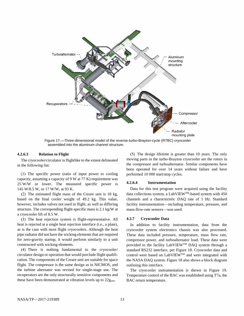
The contract for the cryocooler/circulator was awarded to Creare, Inc. The cryocooler/circulator was modified from the Government-owned Model ACS–2SD two-stage cryocooler that was designed and built by Creare. This unit was owned by the Air Force Research Laboratory (AFRL) at Kirtland Air Force Base. The AFRL agreed that it could be used in this application and eventually transferred ownership of the hardware to NASA. The existing cryocooler was modified by (1) eliminating the second-stage turboalternator and recuperator, (2) replacing the commercial compressor filter and aftercooler with flightlike versions, (3) altering the compressor flow passages for lower flow rates, and (4) repackaging the cryocooler assembly and reconfiguring the tubing, valves, and fittings to interface with the NASA-provided distributed cooling network. Figure 17 shows a three-dimensional model of the modified cryocooler.

4.2.6.2 Operational Characteristics The working fluid was neon, which flowed at a pressure of

~2 atm and a nominal flow rate of 2 g/s. The design cooling capacity is 15 W at a load temperature of 77 K.

The cryocooler was operated by setting the return temperature to a user-specified value. There was no direct feedback to tank pressure, so the cryocooler temperature set point was adjusted manually until the tank pressure was steady. For the pressurization tests, the compressor input power was varied. This approach allowed the available cryocooler (lift) to be varied from ~3 W to over 20 W (at 90 K), which corresponds to a mass flow rate in the system of ~1.5 to 2.5 g/s.

Heat was generated at the compressor and aftercooler, which are both mounted on a common mounting plate. This plate was thermally coupled to the radiator, where the heat was rejected to the cryoshroud. The design heat rejection temperature Trej of the cryocooler was between 270 and 300 K.

NASA/TP—2017-219389 13

Figure 17.—Three-dimensional model of the reverse-turbo-Brayton-cycle (RTBC) cryocooler

assembled into the aluminum channel structure.

4.2.6.3 Relation to Flight The cryocooler/circulator is flightlike to the extent delineated

in the following list:

The specific power (ratio of input power to cooling capacity, assuming a capacity of 9 W at 77 K) requirement was 25 W/W or lower. The measured specific power is 145 W/8.5 W, or 17 W/W, at 93 K.

The estimated flight mass of the Creare unit is 18 kg, based on the final cooler weight of 49.2 kg. This value, however, includes valves not used in flight, as well as differing structure. The corresponding flight-specific mass is 2.1 kg/W at a cryocooler lift of 8.5 W.

The heat rejection system is flight-representative. All heat is rejected at a single heat rejection interface (i.e., a plate), as is the case with most flight cryocoolers. Although the heat pipe radiator did not have the wicking elements that are required for zero-gravity startup, it would perform similarly to a unit constructed with wicking elements.

There is nothing fundamental to the cryocooler/ circulator design or operation that would preclude flight qualifi-cation. The components of the Creare unit are suitable for space flight. The compressor is the same design as in NICMOS, and the turbine alternator was revised for single-stage use. The recuperators are the only structurally sensitive components and these have been demonstrated at vibration levels up to 22grms.

The design lifetime is greater than 10 years. The only moving parts in the turbo-Brayton cryocooler are the rotors in the compressor and turboalternator. Similar components have been operated for over 14 years without failure and have performed 10 000 start/stop cycles.

4.2.6.4 Instrumentation Data for this test program were acquired using the facility

data collections system, a LabVIEWTM-based system with 450 channels and a characteristic DAQ rate of 1 Hz. Standard facility instrumentation—including temperature, pressure, and mass-flow-rate sensors—was used.

4.2.7 Cryocooler Data In addition to facility instrumentation, data from the

cryocooler system electronics chassis was also processed. These data included pressure, temperature, mass flow rate, compressor power, and turboalternator load. These data were provided to the facility LabVIEWTM DAQ system through a standard RS232 interface, per Figure 18. Cryocooler data and control were based on LabVIEWTM and were integrated with the NASA DAQ system. Figure 18 also shows a block diagram outlining this interface.

The cryocooler instrumentation is shown in Figure 19. Temperature control of the BAC was established using T7a, the BAC return temperature.

NASA/TP—2017-219389 14

Figure 18.—Data acquisition (DAQ) schematic.

Figure 19.—Cryocooler instrumentation schematic. BAC, broad-area cooling.

TABLE 5.—ZERO BOILOFF (ZBO) INSTRUMENTATION

Location Count SD/TCa Purpose and notes Diode rake (i.e., liquid temperatures) 8 8/0 Indicate liquid temperature and liquid level Tank wall 13 12/1 Determine exterior tank temperatures at top, bottom, and between cooling loops Broad-area cooling (BAC) system 28 21/7 Measure BAC system temperatures (cooling tubes, manifolds, and thermal

strap) Penetrations 16 6/10 Used in vent, fill/drain, and cap probe heat leak calculations Struts 26 2/24 Used to find tank support heat leak into tank Radiator 25 0/25 Characterize radiator performance Multilayer insulation (MLI) 11 0/11 Determine MLI temperature profile Supports/cabling 12 0/12 Used to find miscellaneous heat leak through wire bundles and suspension

hardware Cryoshroud 18 0/18 Determine boundary temperature Tank pressure 2 N/A Measure and control tank pressure Vacuum chamber pressure 2 N/A Boiloff flow 4 N/A Measure boiloff rates (Teledyne Hastings 200 Series Mass flowmeters) Tank/strut heaters 14 N/A Warm up tank, warm liquid, and set warm boundary temperature on struts aSilicon diode or thermocouple.

4.2.8 Test Tank and Facility In addition to the cryocooler system, the ZBO test article was

highly instrumented. Measurements used for conducting the test series included tank pressure, vacuum chamber pressure, tank liquid and wall temperatures, insulation temperatures,

cryoshroud temperatures, BAC temperatures, and tank boiloff flow rate. Table 5 shows the types of instruments, numbers, and their locations.

A detailed list of research instrumentation is provided in Appendix B.

NASA/TP—2017-219389 15

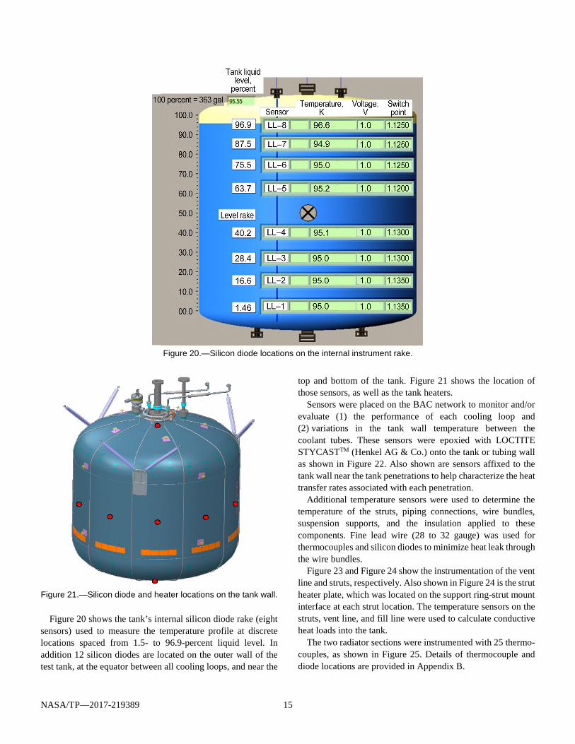
Figure 20.—Silicon diode locations on the internal instrument rake.

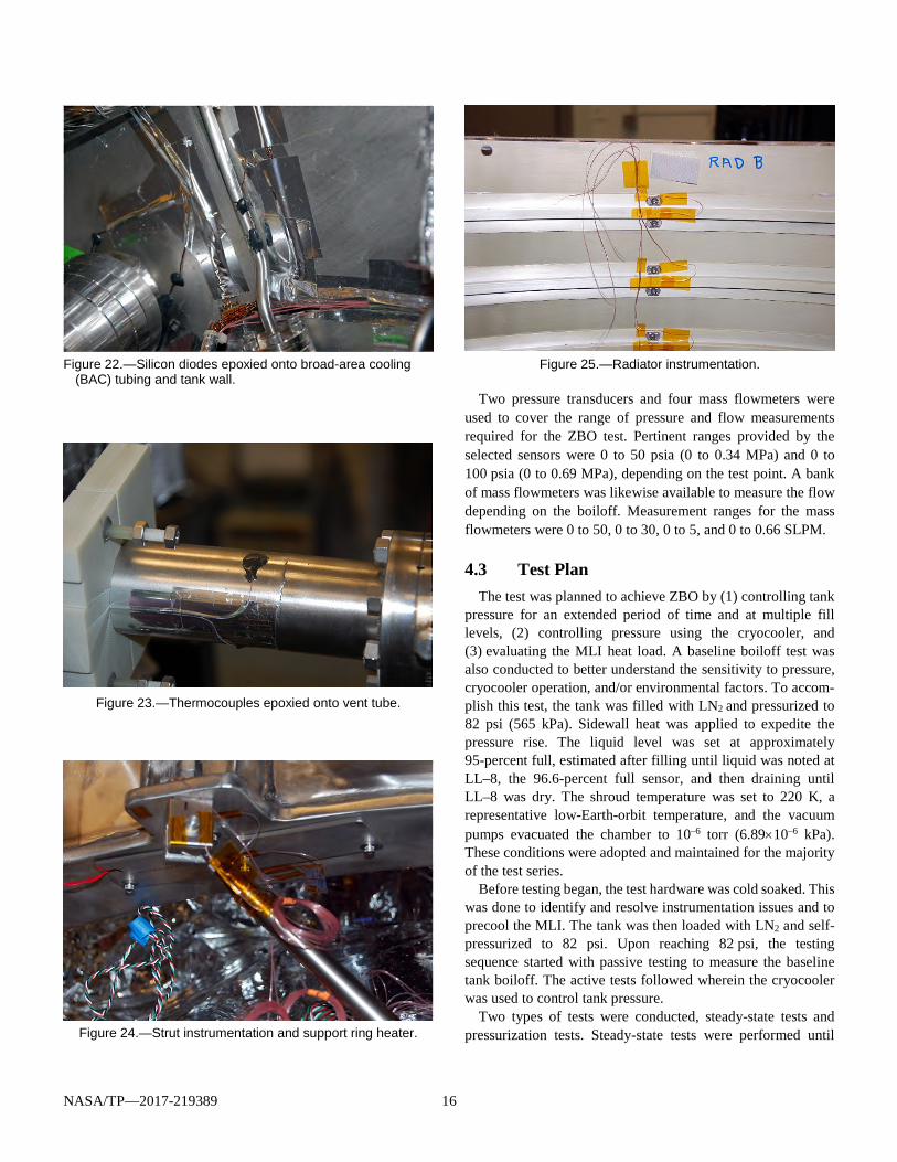
Figure 21.—Silicon diode and heater locations on the tank wall.

Figure 20 shows the tank’s internal silicon diode rake (eight

sensors) used to measure the temperature profile at discrete locations spaced from 1.5- to 96.9-percent liquid level. In addition 12 silicon diodes are located on the outer wall of the test tank, at the equator between all cooling loops, and near the

top and bottom of the tank. Figure 21 shows the location of those sensors, as well as the tank heaters.

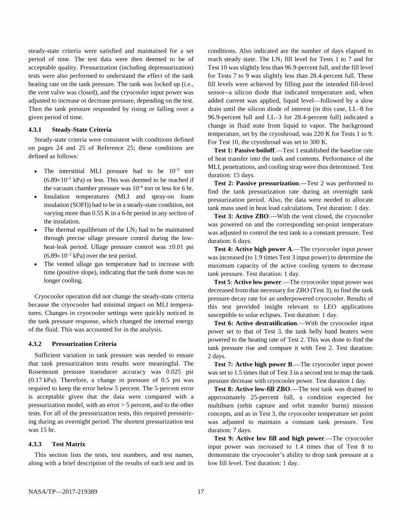
Sensors were placed on the BAC network to monitor and/or evaluate (1) the performance of each cooling loop and (2) variations in the tank wall temperature between the coolant tubes. These sensors were epoxied with LOCTITE STYCASTTM (Henkel AG & Co.) onto the tank or tubing wall as shown in Figure 22. Also shown are sensors affixed to the tank wall near the tank penetrations to help characterize the heat transfer rates associated with each penetration.

Additional temperature sensors were used to determine the temperature of the struts, piping connections, wire bundles, suspension supports, and the insulation applied to these components. Fine lead wire (28 to 32 gauge) was used for thermocouples and silicon diodes to minimize heat leak through the wire bundles.

Figure 23 and Figure 24 show the instrumentation of the vent line and struts, respectively. Also shown in Figure 24 is the strut heater plate, which was located on the support ring-strut mount interface at each strut location. The temperature sensors on the struts, vent line, and fill line were used to calculate conductive heat loads into the tank.

The two radiator sections were instrumented with 25 thermo-couples, as shown in Figure 25. Details of thermocouple and diode locations are provided in Appendix B.

NASA/TP—2017-219389 16

Figure 22.—Silicon diodes epoxied onto broad-area cooling

(BAC) tubing and tank wall.

Figure 23.—Thermocouples epoxied onto vent tube.

Figure 24.—Strut instrumentation and support ring heater.

Figure 25.—Radiator instrumentation.

Two pressure transducers and four mass flowmeters were

used to cover the range of pressure and flow measurements required for the ZBO test. Pertinent ranges provided by the selected sensors were 0 to 50 psia (0 to 0.34 MPa) and 0 to 100 psia (0 to 0.69 MPa), depending on the test point. A bank of mass flowmeters was likewise available to measure the flow depending on the boiloff. Measurement ranges for the mass flowmeters were 0 to 50, 0 to 30, 0 to 5, and 0 to 0.66 SLPM.

4.3 Test Plan The test was planned to achieve ZBO by (1) controlling tank

pressure for an extended period of time and at multiple fill levels, (2) controlling pressure using the cryocooler, and (3) evaluating the MLI heat load. A baseline boiloff test was also conducted to better understand the sensitivity to pressure, cryocooler operation, and/or environmental factors. To accom-plish this test, the tank was filled with LN2 and pressurized to 82 psi (565 kPa). Sidewall heat was applied to expedite the pressure rise. The liquid level was set at approximately 95-percent full, estimated after filling until liquid was noted at LL–8, the 96.6-percent full sensor, and then draining until LL–8 was dry. The shroud temperature was set to 220 K, a representative low-Earth-orbit temperature, and the vacuum pumps evacuated the chamber to 10–6 torr (6.89×10–6 kPa). These conditions were adopted and maintained for the majority of the test series.

Before testing began, the test hardware was cold soaked. This was done to identify and resolve instrumentation issues and to precool the MLI. The tank was then loaded with LN2 and self-pressurized to 82 psi. Upon reaching 82 psi, the testing sequence started with passive testing to measure the baseline tank boiloff. The active tests followed wherein the cryocooler was used to control tank pressure.

Two types of tests were conducted, steady-state tests and pressurization tests. Steady-state tests were performed until

NASA/TP—2017-219389 17

steady-state criteria were satisfied and maintained for a set period of time. The test data were then deemed to be of acceptable quality. Pressurization (including depressurization) tests were also performed to understand the effect of the tank heating rate on the tank pressure. The tank was locked up (i.e., the vent valve was closed), and the cryocooler input power was adjusted to increase or decrease pressure, depending on the test. Then the tank pressure responded by rising or falling over a given period of time.

4.3.1 Steady-State Criteria Steady-state criteria were consistent with conditions defined

on pages 24 and 25 of Reference 25; these conditions are defined as follows:

• The interstitial MLI pressure had to be 10–5 torr

(6.89×10–5 kPa) or less. This was deemed to be reached if the vacuum chamber pressure was 10–6 torr or less for 6 hr.

• Insulation temperatures (MLI and spray-on foam insulation (SOFI)) had to be in a steady-state condition, not varying more than 0.55 K in a 6-hr period in any section of the insulation.

• The thermal equilibrium of the LN2 had to be maintained through precise ullage pressure control during the low-heat-leak period. Ullage pressure control was ±0.01 psi (6.89×10–2 kPa) over the test period.

• The vented ullage gas temperature had to increase with time (positive slope), indicating that the tank dome was no longer cooling.

Cryocooler operation did not change the steady-state criteria

because the cryocooler had minimal impact on MLI tempera-tures. Changes in cryocooler settings were quickly noticed in the tank pressure response, which changed the internal energy of the fluid. This was accounted for in the analysis.

4.3.2 Pressurization Criteria

Sufficient variation in tank pressure was needed to ensure that tank pressurization tests results were meaningful. The Rosemount pressure transducer accuracy was 0.025 psi (0.17 kPa). Therefore, a change in pressure of 0.5 psi was required to keep the error below 5 percent. The 5-percent error is acceptable given that the data were compared with a pressurization model, with an error > 5 percent, and to the other tests. For all of the pressurization tests, this required pressuriz-ing during an overnight period. The shortest pressurization test was 15 hr.

4.3.3 Test Matrix This section lists the tests, test numbers, and test names,

along with a brief description of the results of each test and its

conditions. Also indicated are the number of days elapsed to reach steady state. The LN2 fill level for Tests 1 to 7 and for Test 10 was slightly less than 96.9-percent full, and the fill level for Tests 7 to 9 was slightly less than 28.4-percent full. These fill levels were achieved by filling past the intended fill-level sensor--a silicon diode that indicated temperature and, when added current was applied, liquid level—followed by a slow drain until the silicon diode of interest (in this case, LL–8 for 96.9-percent full and LL–3 for 28.4-percent full) indicated a change in fluid state from liquid to vapor. The background temperature, set by the cryoshroud, was 220 K for Tests 1 to 9. For Test 10, the cryoshroud was set to 300 K.

Test 1: Passive boiloff.—Test 1 established the baseline rate of heat transfer into the tank and contents. Performance of the MLI, penetrations, and cooling strap were thus determined. Test duration: 15 days.

Test 2: Passive pressurization.—Test 2 was performed to find the tank pressurization rate during an overnight tank pressurization period. Also, the data were needed to allocate tank mass used in heat load calculations. Test duration: 1 day.

Test 3: Active ZBO.—With the vent closed, the cryocooler was powered on and the corresponding set-point temperature was adjusted to control the test tank to a constant pressure. Test duration: 6 days.

Test 4: Active high power A.—The cryocooler input power was increased (to 1.9 times Test 3 input power) to determine the maximum capacity of the active cooling system to decrease tank pressure. Test duration: 1 day.

Test 5: Active low power.—The cryocooler input power was decreased from that necessary for ZBO (Test 3), to find the tank pressure decay rate for an underpowered cryocooler. Results of this test provided insight relevant to LEO applications susceptible to solar eclipses. Test duration: 1 day.

Test 6: Active destratification.—With the cryocooler input power set to that of Test 3, the tank belly band heaters were powered to the heating rate of Test 2. This was done to find the tank pressure rise and compare it with Test 2. Test duration: 2 days.

Test 7: Active high power B.—The cryocooler input power was set to 1.5 times that of Test 3 in a second test to map the tank pressure decrease with cryocooler power. Test duration 1 day.

Test 8: Active low-fill ZBO.—The test tank was drained to approximately 25-percent full, a condition expected for multiburn (orbit capture and orbit transfer burns) mission concepts, and as in Test 3, the cryocooler temperature set point was adjusted to maintain a constant tank pressure. Test duration: 7 days.

Test 9: Active low fill and high power.—The cryocooler input power was increased to 1.4 times that of Test 8 to demonstrate the cryocooler’s ability to drop tank pressure at a low fill level. Test duration: 1 day.

NASA/TP—2017-219389 18

Test 10: Passive boiloff at 300 K.—With the cryoshroud setting changed to 300 K and the cryocooler turned off, a second passive test was performed to provide a second data point pertinent to MLI performance. Test duration: 10 days.

The cryocooler was operated continuously from Test 3 to 9 for 19 days, and during that time, the test tank was not vented. Extended, continuous operation of the cryocooler was important to gain confidence in the ZBO system.

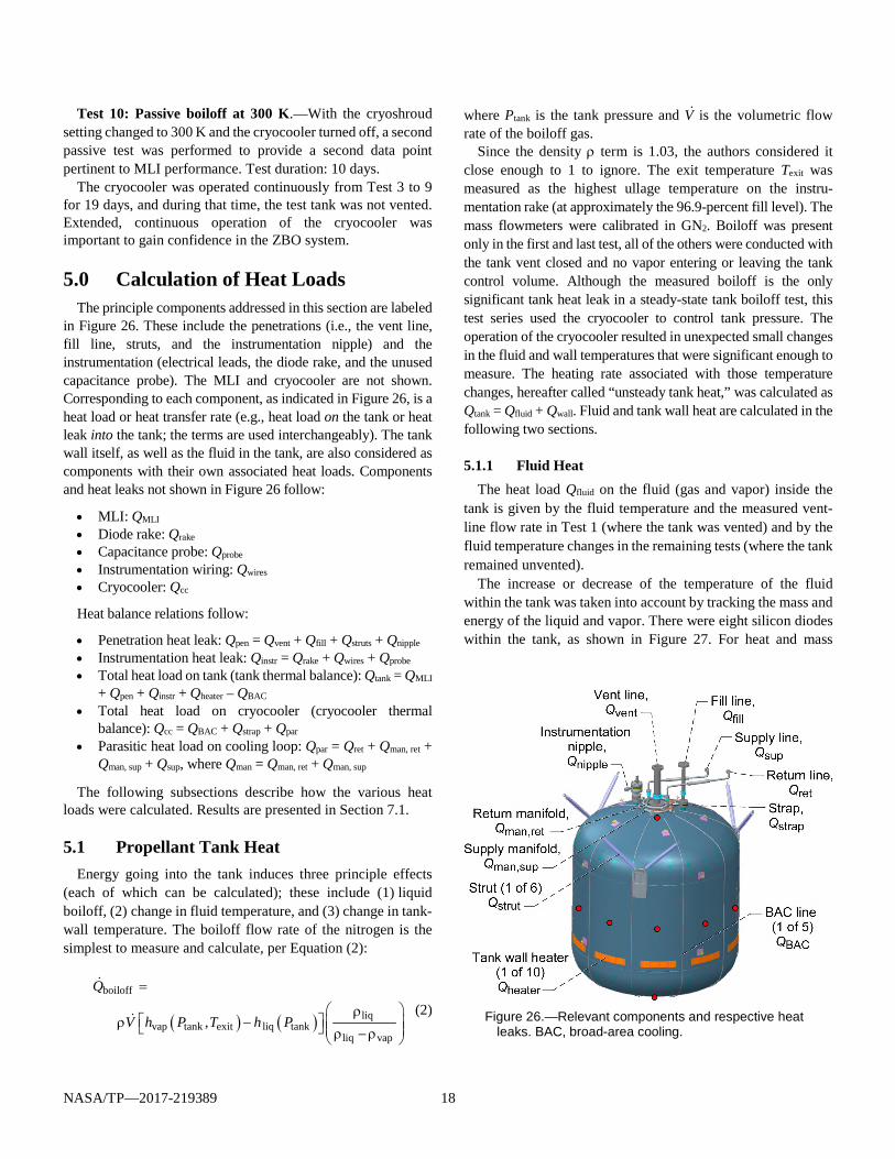
5.0 Calculation of Heat Loads The principle components addressed in this section are labeled

in Figure 26. These include the penetrations (i.e., the vent line, fill line, struts, and the instrumentation nipple) and the instrumentation (electrical leads, the diode rake, and the unused capacitance probe). The MLI and cryocooler are not shown. Corresponding to each component, as indicated in Figure 26, is a heat load or heat transfer rate (e.g., heat load on the tank or heat leak into the tank; the terms are used interchangeably). The tank wall itself, as well as the fluid in the tank, are also considered as components with their own associated heat loads. Components and heat leaks not shown in Figure 26 follow:

• MLI: QMLI • Diode rake: Qrake • Capacitance probe: Qprobe • Instrumentation wiring: Qwires • Cryocooler: Qcc

Heat balance relations follow:

• Penetration heat leak: Qpen = Qvent + Qfill + Qstruts + Qnipple • Instrumentation heat leak: Qinstr = Qrake + Qwires + Qprobe • Total heat load on tank (tank thermal balance): Qtank = QMLI

+ Qpen + Qinstr + Qheater – QBAC • Total heat load on cryocooler (cryocooler thermal

balance): Qcc = QBAC + Qstrap + Qpar • Parasitic heat load on cooling loop: Qpar = Qret + Qman, ret +

Qman, sup + Qsup, where Qman = Qman, ret + Qman, sup

The following subsections describe how the various heat loads were calculated. Results are presented in Section 7.1.

5.1 Propellant Tank Heat Energy going into the tank induces three principle effects

(each of which can be calculated); these include (1) liquid boiloff, (2) change in fluid temperature, and (3) change in tank-wall temperature. The boiloff flow rate of the nitrogen is the simplest to measure and calculate, per Equation (2):

( ) ( )

boiloff

liqvap tank exit liq tank

liq vap,

Q

V h P T h P

=

ρ ρ − ρ − ρ

(2)

where Ptank is the tank pressure and V is the volumetric flow rate of the boiloff gas.

Since the density ρ term is 1.03, the authors considered it close enough to 1 to ignore. The exit temperature Texit was measured as the highest ullage temperature on the instru-mentation rake (at approximately the 96.9-percent fill level). The mass flowmeters were calibrated in GN2. Boiloff was present only in the first and last test, all of the others were conducted with the tank vent closed and no vapor entering or leaving the tank control volume. Although the measured boiloff is the only significant tank heat leak in a steady-state tank boiloff test, this test series used the cryocooler to control tank pressure. The operation of the cryocooler resulted in unexpected small changes in the fluid and wall temperatures that were significant enough to measure. The heating rate associated with those temperature changes, hereafter called “unsteady tank heat,” was calculated as Qtank = Qfluid + Qwall. Fluid and tank wall heat are calculated in the following two sections.

5.1.1 Fluid Heat The heat load Qfluid on the fluid (gas and vapor) inside the

tank is given by the fluid temperature and the measured vent-line flow rate in Test 1 (where the tank was vented) and by the fluid temperature changes in the remaining tests (where the tank remained unvented).

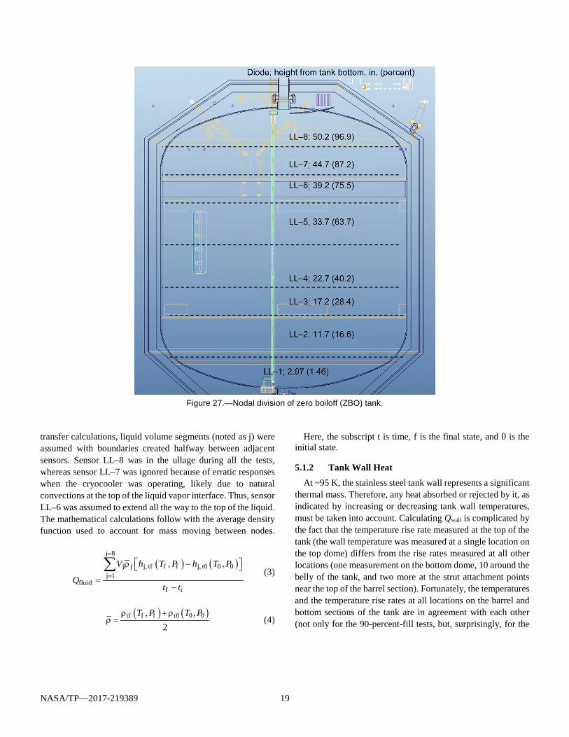
The increase or decrease of the temperature of the fluid within the tank was taken into account by tracking the mass and energy of the liquid and vapor. There were eight silicon diodes within the tank, as shown in Figure 27. For heat and mass

Figure 26.—Relevant components and respective heat

leaks. BAC, broad-area cooling.

NASA/TP—2017-219389 19

Figure 27.—Nodal division of zero boiloff (ZBO) tank.

transfer calculations, liquid volume segments (noted as j) were assumed with boundaries created halfway between adjacent sensors. Sensor LL–8 was in the ullage during all the tests, whereas sensor LL–7 was ignored because of erratic responses when the cryocooler was operating, likely due to natural convections at the top of the liquid vapor interface. Thus, sensor LL–6 was assumed to extend all the way to the top of the liquid. The mathematical calculations follow with the average density function used to account for mass moving between nodes.

( ) ( )

j 8

j j j, tf f f j, t0 0 0j 1

fluidf i

, ,V h T P h T P

Qt t

=

=

ρ − =

−

∑

(3)

( ) ( )tf f f t0 0 0, ,2

T P T Pρ + ρρ = (4)

Here, the subscript t is time, f is the final state, and 0 is the initial state.

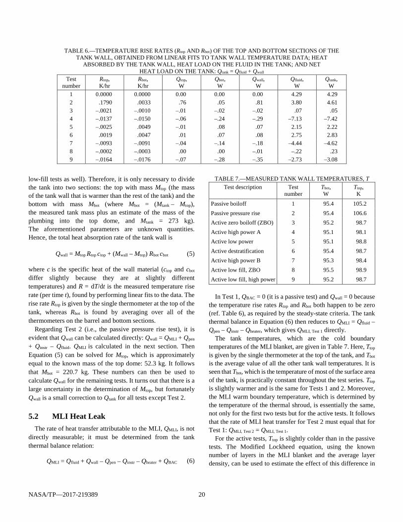
5.1.2 Tank Wall Heat At ~95 K, the stainless steel tank wall represents a significant

thermal mass. Therefore, any heat absorbed or rejected by it, as indicated by increasing or decreasing tank wall temperatures, must be taken into account. Calculating Qwall is complicated by the fact that the temperature rise rate measured at the top of the tank (the wall temperature was measured at a single location on the top dome) differs from the rise rates measured at all other locations (one measurement on the bottom dome, 10 around the belly of the tank, and two more at the strut attachment points near the top of the barrel section). Fortunately, the temperatures and the temperature rise rates at all locations on the barrel and bottom sections of the tank are in agreement with each other (not only for the 90-percent-fill tests, but, surprisingly, for the

NASA/TP—2017-219389 20

TABLE 6.—TEMPERATURE RISE RATES (Rtop AND Rbot) OF THE TOP AND BOTTOM SECTIONS OF THE TANK WALL, OBTAINED FROM LINEAR FITS TO TANK WALL TEMPERATURE DATA; HEAT

ABSORBED BY THE TANK WALL, HEAT LOAD ON THE FLUID IN THE TANK; AND NET HEAT LOAD ON THE TANK: Qtank = Qfluid + Qwall

Test number

Rtop, K/hr

Rbot, K/hr

Qtop, W

Qbot, W

Qwall, W

Qfluid, W

Qtank, W

1 0.0000 0.0000 0.00 0.00 0.00 4.29 4.29 2 .1790 .0033 .76 .05 .81 3.80 4.61 3 –.0021 –.0010 –.01 –.02 –.02 .07 .05 4 –.0137 –.0150 –.06 –.24 –.29 –7.13 –7.42 5 –.0025 .0049 –.01 .08 .07 2.15 2.22 6 .0019 .0047 .01 .07 .08 2.75 2.83 7 –.0093 –.0091 –.04 –.14 –.18 –4.44 –4.62 8 –.0002 –.0003 .00 .00 –.01 –.22 .23 9 –.0164 –.0176 –.07 –.28 –.35 –2.73 –3.08

low-fill tests as well). Therefore, it is only necessary to divide the tank into two sections: the top with mass Mtop (the mass of the tank wall that is warmer than the rest of the tank) and the bottom with mass Mbot (where Mbot = (Mtank – Mtop), the measured tank mass plus an estimate of the mass of the plumbing into the top dome, and Mtank = 273 kg). The aforementioned parameters are unknown quantities. Hence, the total heat absorption rate of the tank wall is

Qwall = Mtop Rtop ctop + (Mwall – Mtop) Rbot cbot (5)

where c is the specific heat of the wall material (ctop and cbot differ slightly because they are at slightly different temperatures) and R = dT/dt is the measured temperature rise rate (per time t), found by performing linear fits to the data. The rise rate Rtop is given by the single thermometer at the top of the tank, whereas Rbot is found by averaging over all of the thermometers on the barrel and bottom sections.

Regarding Test 2 (i.e., the passive pressure rise test), it is evident that Qwall can be calculated directly: Qwall = QMLI + Qpen + Qinstr – Qfluid. QMLI is calculated in the next section. Then Equation (5) can be solved for Mtop, which is approximately equal to the known mass of the top dome: 52.3 kg. It follows that Mbot = 220.7 kg. These numbers can then be used to calculate Qwall for the remaining tests. It turns out that there is a large uncertainty in the determination of Mtop, but fortunately Qwall is a small correction to Qtank for all tests except Test 2.

5.2 MLI Heat Leak The rate of heat transfer attributable to the MLI, QMLI, is not

directly measurable; it must be determined from the tank thermal balance relation:

QMLI = Qfluid + Qwall – Qpen – Qinstr – Qheater + QBAC (6)

TABLE 7.—MEASURED TANK WALL TEMPERATURES, T Test description Test

number Tbot, W

Ttop, K

Passive boiloff 1 95.4 105.2 Passive pressure rise 2 95.4 106.6 Active zero boiloff (ZBO) 3 95.2 98.7 Active high power A 4 95.1 98.1 Active low power 5 95.1 98.8 Active destratification 6 95.4 98.7 Active high power B 7 95.3 98.4 Active low fill, ZBO 8 95.5 98.9 Active low fill, high power 9 95.2 98.7

In Test 1, QBAC = 0 (it is a passive test) and Qwall = 0 because

the temperature rise rates Rtop and Rbot both happen to be zero (ref. Table 6), as required by the steady-state criteria. The tank thermal balance in Equation (6) then reduces to QMLI = Qfluid – Qpen – Qinstr – Qheater, which gives QMLI, Test 1 directly.

The tank temperatures, which are the cold boundary temperatures of the MLI blanket, are given in Table 7. Here, Ttop is given by the single thermometer at the top of the tank, and Tbot is the average value of all the other tank wall temperatures. It is seen that Tbot, which is the temperature of most of the surface area of the tank, is practically constant throughout the test series. Ttop is slightly warmer and is the same for Tests 1 and 2. Moreover, the MLI warm boundary temperature, which is determined by the temperature of the thermal shroud, is essentially the same, not only for the first two tests but for the active tests. It follows that the rate of MLI heat transfer for Test 2 must equal that for Test 1: QMLI, Test 2 = QMLI, Test 1.

For the active tests, Ttop is slightly colder than in the passive tests. The Modified Lockheed equation, using the known number of layers in the MLI blanket and the average layer density, can be used to estimate the effect of this difference in

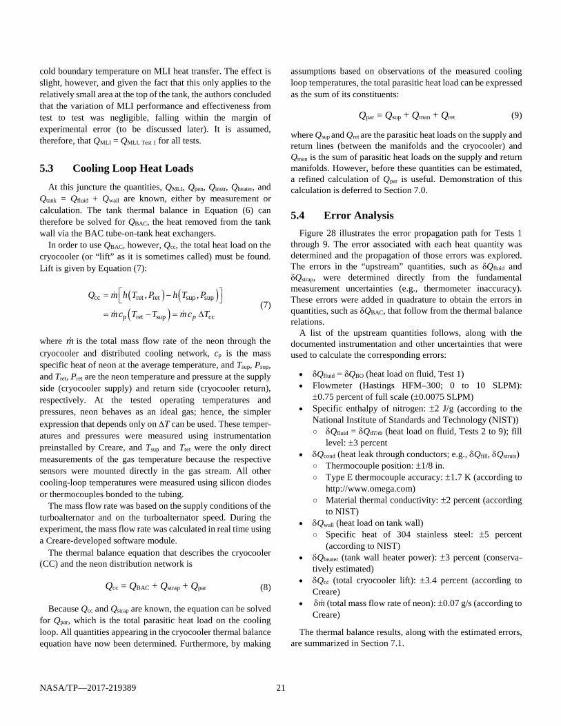
NASA/TP—2017-219389 21

cold boundary temperature on MLI heat transfer. The effect is slight, however, and given the fact that this only applies to the relatively small area at the top of the tank, the authors concluded that the variation of MLI performance and effectiveness from test to test was negligible, falling within the margin of experimental error (to be discussed later). It is assumed, therefore, that QMLI = QMLI, Test 1 for all tests.

5.3 Cooling Loop Heat Loads At this juncture the quantities, QMLI, Qpen, Qinstr, Qheater, and

Qtank = Qfluid + Qwall are known, either by measurement or calculation. The tank thermal balance in Equation (6) can therefore be solved for QBAC, the heat removed from the tank wall via the BAC tube-on-tank heat exchangers.

In order to use QBAC, however, Qcc, the total heat load on the cryocooler (or “lift” as it is sometimes called) must be found. Lift is given by Equation (7):

( ) ( )( )

cc ret ret sup sup

p ret sup cc

, ,

p

Q m h T P h T P

mc T T mc T

= −

= − = ∆

(7)

where m is the total mass flow rate of the neon through the cryocooler and distributed cooling network, cp is the mass specific heat of neon at the average temperature, and Tsup, Psup, and Tret, Pret are the neon temperature and pressure at the supply side (cryocooler supply) and return side (cryocooler return), respectively. At the tested operating temperatures and pressures, neon behaves as an ideal gas; hence, the simpler expression that depends only on ∆T can be used. These temper-atures and pressures were measured using instrumentation preinstalled by Creare, and Tsup and Tret were the only direct measurements of the gas temperature because the respective sensors were mounted directly in the gas stream. All other cooling-loop temperatures were measured using silicon diodes or thermocouples bonded to the tubing.

The mass flow rate was based on the supply conditions of the turboalternator and on the turboalternator speed. During the experiment, the mass flow rate was calculated in real time using a Creare-developed software module.

The thermal balance equation that describes the cryocooler (CC) and the neon distribution network is

Qcc = QBAC + Qstrap + Qpar (8)

Because Qcc and Qstrap are known, the equation can be solved for Qpar, which is the total parasitic heat load on the cooling loop. All quantities appearing in the cryocooler thermal balance equation have now been determined. Furthermore, by making

assumptions based on observations of the measured cooling loop temperatures, the total parasitic heat load can be expressed as the sum of its constituents:

Qpar = Qsup + Qman + Qret (9)

where Qsup and Qret are the parasitic heat loads on the supply and return lines (between the manifolds and the cryocooler) and Qman is the sum of parasitic heat loads on the supply and return manifolds. However, before these quantities can be estimated, a refined calculation of Qpar is useful. Demonstration of this calculation is deferred to Section 7.0.

5.4 Error Analysis Figure 28 illustrates the error propagation path for Tests 1

through 9. The error associated with each heat quantity was determined and the propagation of those errors was explored. The errors in the “upstream” quantities, such as δQfluid and δQstrap, were determined directly from the fundamental measurement uncertainties (e.g., thermometer inaccuracy). These errors were added in quadrature to obtain the errors in quantities, such as δQBAC, that follow from the thermal balance relations.

A list of the upstream quantities follows, along with the documented instrumentation and other uncertainties that were used to calculate the corresponding errors:

• δQfluid = δQBO (heat load on fluid, Test 1) • Flowmeter (Hastings HFM–300; 0 to 10 SLPM):

±0.75 percent of full scale (±0.0075 SLPM) • Specific enthalpy of nitrogen: ±2 J/g (according to the

National Institute of Standards and Technology (NIST)) ○ δQfluid = δQdT/dt (heat load on fluid, Tests 2 to 9); fill

level: ±3 percent • δQcond (heat leak through conductors; e.g., δQfill, δQstruts)

○ Thermocouple position: ±1/8 in. ○ Type E thermocouple accuracy: ±1.7 K (according to

http://www.omega.com) ○ Material thermal conductivity: ±2 percent (according

to NIST) • δQwall (heat load on tank wall)

○ Specific heat of 304 stainless steel: ±5 percent (according to NIST)

• δQheater (tank wall heater power): ±3 percent (conserva-tively estimated)

• δQcc (total cryocooler lift): ±3.4 percent (according to Creare)

• mδ (total mass flow rate of neon): ±0.07 g/s (according to Creare)

The thermal balance results, along with the estimated errors, are summarized in Section 7.1.

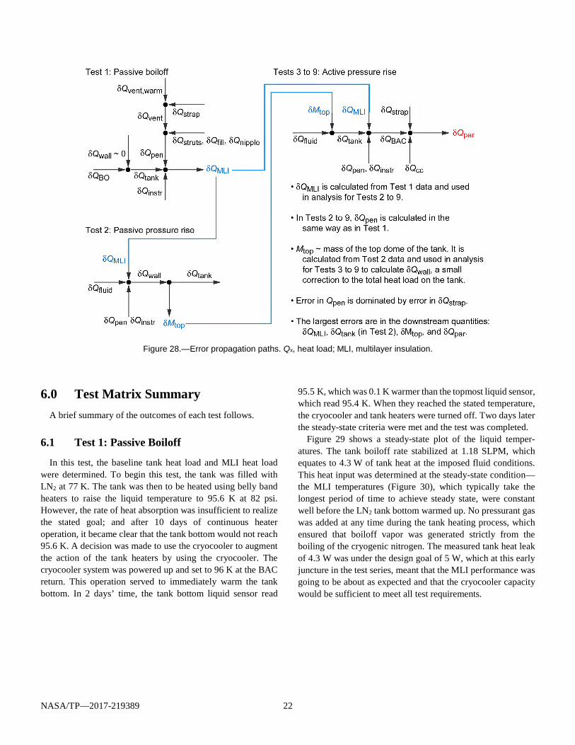
NASA/TP—2017-219389 22

Figure 28.—Error propagation paths. Qx, heat load; MLI, multilayer insulation.

6.0 Test Matrix Summary

A brief summary of the outcomes of each test follows.

6.1 Test 1: Passive Boiloff

In this test, the baseline tank heat load and MLI heat load were determined. To begin this test, the tank was filled with LN2 at 77 K. The tank was then to be heated using belly band heaters to raise the liquid temperature to 95.6 K at 82 psi. However, the rate of heat absorption was insufficient to realize the stated goal; and after 10 days of continuous heater operation, it became clear that the tank bottom would not reach 95.6 K. A decision was made to use the cryocooler to augment the action of the tank heaters by using the cryocooler. The cryocooler system was powered up and set to 96 K at the BAC return. This operation served to immediately warm the tank bottom. In 2 days’ time, the tank bottom liquid sensor read

95.5 K, which was 0.1 K warmer than the topmost liquid sensor, which read 95.4 K. When they reached the stated temperature, the cryocooler and tank heaters were turned off. Two days later the steady-state criteria were met and the test was completed.

Figure 29 shows a steady-state plot of the liquid temper-atures. The tank boiloff rate stabilized at 1.18 SLPM, which equates to 4.3 W of tank heat at the imposed fluid conditions. This heat input was determined at the steady-state condition—the MLI temperatures (Figure 30), which typically take the longest period of time to achieve steady state, were constant well before the LN2 tank bottom warmed up. No pressurant gas was added at any time during the tank heating process, which ensured that boiloff vapor was generated strictly from the boiling of the cryogenic nitrogen. The measured tank heat leak of 4.3 W was under the design goal of 5 W, which at this early juncture in the test series, meant that the MLI performance was going to be about as expected and that the cryocooler capacity would be sufficient to meet all test requirements.

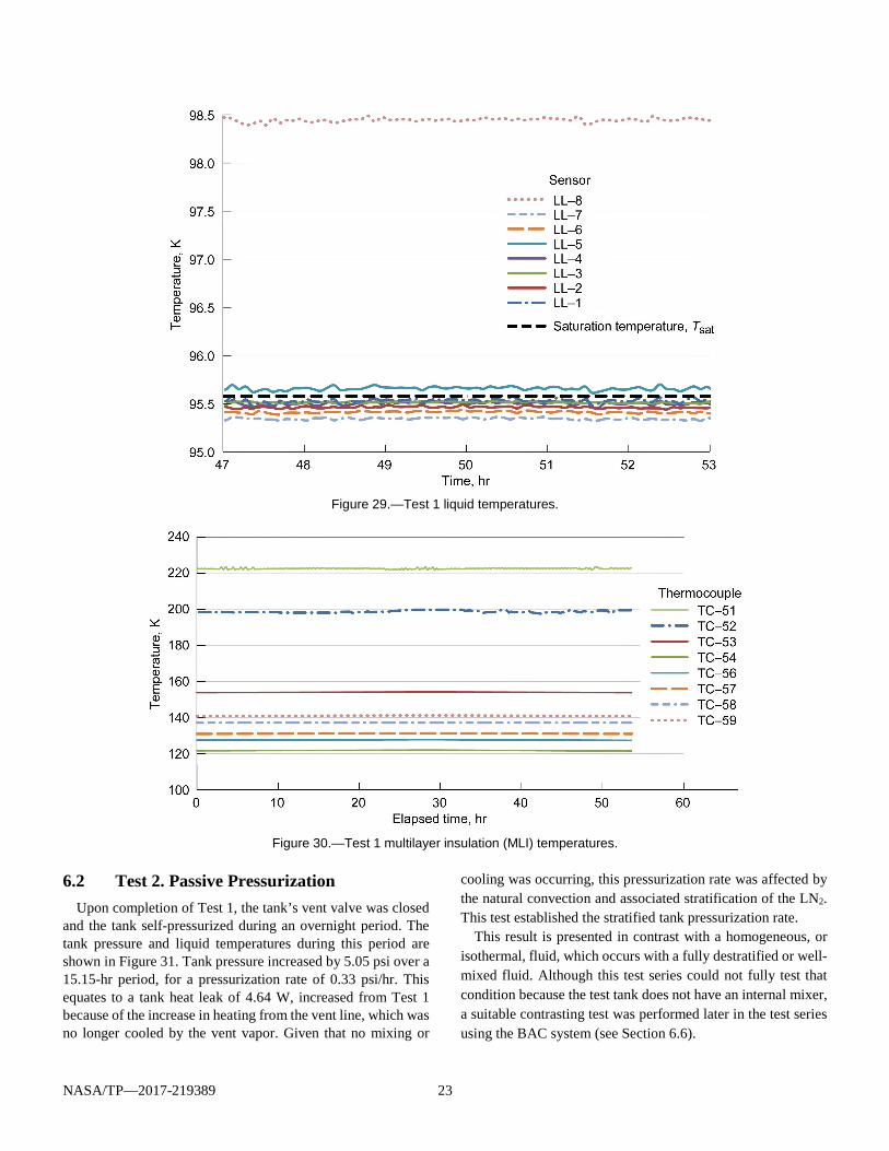
NASA/TP—2017-219389 23

Figure 29.—Test 1 liquid temperatures.

Figure 30.—Test 1 multilayer insulation (MLI) temperatures.

6.2 Test 2. Passive Pressurization

Upon completion of Test 1, the tank’s vent valve was closed and the tank self-pressurized during an overnight period. The tank pressure and liquid temperatures during this period are shown in Figure 31. Tank pressure increased by 5.05 psi over a 15.15-hr period, for a pressurization rate of 0.33 psi/hr. This equates to a tank heat leak of 4.64 W, increased from Test 1 because of the increase in heating from the vent line, which was no longer cooled by the vent vapor. Given that no mixing or

cooling was occurring, this pressurization rate was affected by the natural convection and associated stratification of the LN2. This test established the stratified tank pressurization rate.

This result is presented in contrast with a homogeneous, or isothermal, fluid, which occurs with a fully destratified or well-mixed fluid. Although this test series could not fully test that condition because the test tank does not have an internal mixer, a suitable contrasting test was performed later in the test series using the BAC system (see Section 6.6).

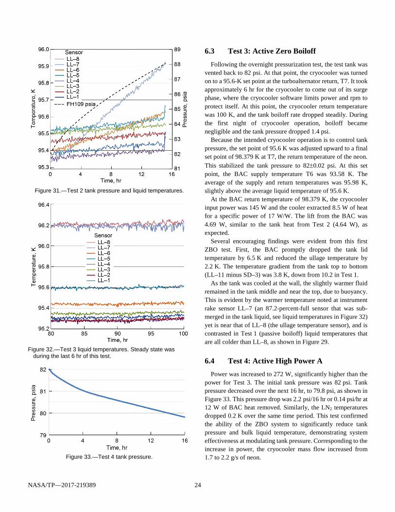
NASA/TP—2017-219389 24

Figure 31.—Test 2 tank pressure and liquid temperatures.

Figure 32.—Test 3 liquid temperatures. Steady state was

during the last 6 hr of this test.

Figure 33.—Test 4 tank pressure.

6.3 Test 3: Active Zero Boiloff

Following the overnight pressurization test, the test tank was vented back to 82 psi. At that point, the cryocooler was turned on to a 95.6-K set point at the turboalternator return, T7. It took approximately 6 hr for the cryocooler to come out of its surge phase, where the cryocooler software limits power and rpm to protect itself. At this point, the cryocooler return temperature was 100 K, and the tank boiloff rate dropped steadily. During the first night of cryocooler operation, boiloff became negligible and the tank pressure dropped 1.4 psi.

Because the intended cryocooler operation is to control tank pressure, the set point of 95.6 K was adjusted upward to a final set point of 98.379 K at T7, the return temperature of the neon. This stabilized the tank pressure to 82±0.02 psi. At this set point, the BAC supply temperature T6 was 93.58 K. The average of the supply and return temperatures was 95.98 K, slightly above the average liquid temperature of 95.6 K.

At the BAC return temperature of 98.379 K, the cryocooler input power was 145 W and the cooler extracted 8.5 W of heat for a specific power of 17 W/W. The lift from the BAC was 4.69 W, similar to the tank heat from Test 2 (4.64 W), as expected.

Several encouraging findings were evident from this first ZBO test. First, the BAC promptly dropped the tank lid temperature by 6.5 K and reduced the ullage temperature by 2.2 K. The temperature gradient from the tank top to bottom (LL–11 minus SD–3) was 3.8 K, down from 10.2 in Test 1.

As the tank was cooled at the wall, the slightly warmer fluid remained in the tank middle and near the top, due to buoyancy. This is evident by the warmer temperature noted at instrument rake sensor LL–7 (an 87.2-percent-full sensor that was sub-merged in the tank liquid, see liquid temperatures in Figure 32) yet is near that of LL–8 (the ullage temperature sensor), and is contrasted in Test 1 (passive boiloff) liquid temperatures that are all colder than LL–8, as shown in Figure 29.

6.4 Test 4: Active High Power A Power was increased to 272 W, significantly higher than the

power for Test 3. The initial tank pressure was 82 psi. Tank pressure decreased over the next 16 hr, to 79.8 psi, as shown in Figure 33. This pressure drop was 2.2 psi/16 hr or 0.14 psi/hr at 12 W of BAC heat removed. Similarly, the LN2 temperatures dropped 0.2 K over the same time period. This test confirmed the ability of the ZBO system to significantly reduce tank pressure and bulk liquid temperature, demonstrating system effectiveness at modulating tank pressure. Corresponding to the increase in power, the cryocooler mass flow increased from 1.7 to 2.2 g/s of neon.

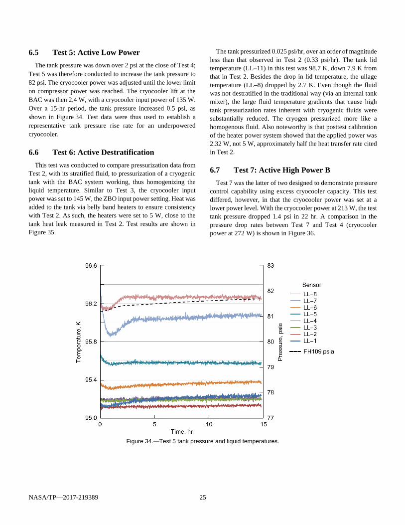
NASA/TP—2017-219389 25

6.5 Test 5: Active Low Power The tank pressure was down over 2 psi at the close of Test 4;

Test 5 was therefore conducted to increase the tank pressure to 82 psi. The cryocooler power was adjusted until the lower limit on compressor power was reached. The cryocooler lift at the BAC was then 2.4 W, with a cryocooler input power of 135 W. Over a 15-hr period, the tank pressure increased 0.5 psi, as shown in Figure 34. Test data were thus used to establish a representative tank pressure rise rate for an underpowered cryocooler.

6.6 Test 6: Active Destratification This test was conducted to compare pressurization data from

Test 2, with its stratified fluid, to pressurization of a cryogenic tank with the BAC system working, thus homogenizing the liquid temperature. Similar to Test 3, the cryocooler input power was set to 145 W, the ZBO input power setting. Heat was added to the tank via belly band heaters to ensure consistency with Test 2. As such, the heaters were set to 5 W, close to the tank heat leak measured in Test 2. Test results are shown in Figure 35.

The tank pressurized 0.025 psi/hr, over an order of magnitude less than that observed in Test 2 (0.33 psi/hr). The tank lid temperature (LL–11) in this test was 98.7 K, down 7.9 K from that in Test 2. Besides the drop in lid temperature, the ullage temperature (LL–8) dropped by 2.7 K. Even though the fluid was not destratified in the traditional way (via an internal tank mixer), the large fluid temperature gradients that cause high tank pressurization rates inherent with cryogenic fluids were substantially reduced. The cryogen pressurized more like a homogenous fluid. Also noteworthy is that posttest calibration of the heater power system showed that the applied power was 2.32 W, not 5 W, approximately half the heat transfer rate cited in Test 2.

6.7 Test 7: Active High Power B Test 7 was the latter of two designed to demonstrate pressure

control capability using excess cryocooler capacity. This test differed, however, in that the cryocooler power was set at a lower power level. With the cryocooler power at 213 W, the test tank pressure dropped 1.4 psi in 22 hr. A comparison in the pressure drop rates between Test 7 and Test 4 (cryocooler power at 272 W) is shown in Figure 36.

Figure 34.—Test 5 tank pressure and liquid temperatures.

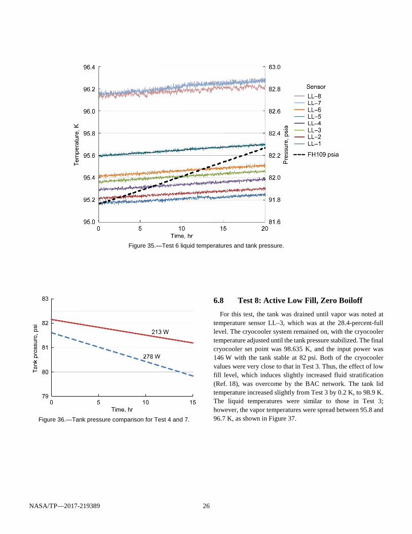
NASA/TP—2017-219389 26

Figure 35.—Test 6 liquid temperatures and tank pressure.

Figure 36.—Tank pressure comparison for Test 4 and 7.

6.8 Test 8: Active Low Fill, Zero Boiloff For this test, the tank was drained until vapor was noted at

temperature sensor LL–3, which was at the 28.4-percent-full level. The cryocooler system remained on, with the cryocooler temperature adjusted until the tank pressure stabilized. The final cryocooler set point was 98.635 K, and the input power was 146 W with the tank stable at 82 psi. Both of the cryocooler values were very close to that in Test 3. Thus, the effect of low fill level, which induces slightly increased fluid stratification (Ref. 18), was overcome by the BAC network. The tank lid temperature increased slightly from Test 3 by 0.2 K, to 98.9 K. The liquid temperatures were similar to those in Test 3; however, the vapor temperatures were spread between 95.8 and 96.7 K, as shown in Figure 37.

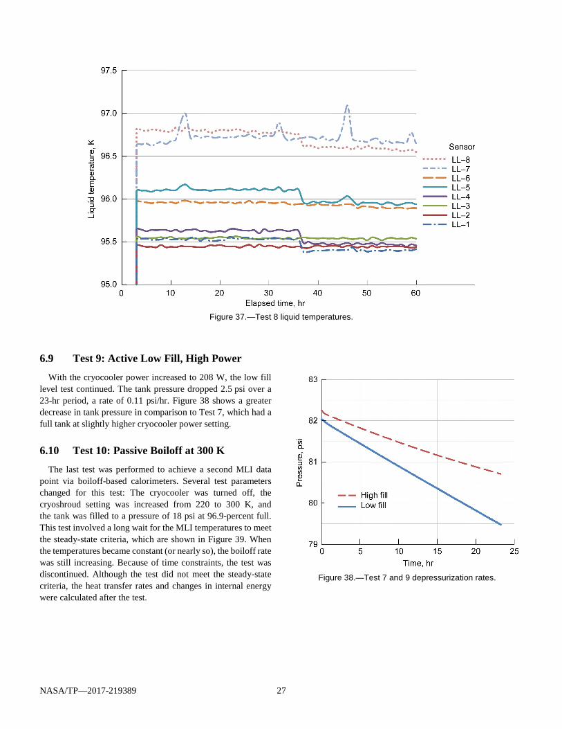
NASA/TP—2017-219389 27

Figure 37.—Test 8 liquid temperatures.

6.9 Test 9: Active Low Fill, High Power With the cryocooler power increased to 208 W, the low fill

level test continued. The tank pressure dropped 2.5 psi over a 23-hr period, a rate of 0.11 psi/hr. Figure 38 shows a greater decrease in tank pressure in comparison to Test 7, which had a full tank at slightly higher cryocooler power setting.

6.10 Test 10: Passive Boiloff at 300 K The last test was performed to achieve a second MLI data

point via boiloff-based calorimeters. Several test parameters changed for this test: The cryocooler was turned off, the cryoshroud setting was increased from 220 to 300 K, and the tank was filled to a pressure of 18 psi at 96.9-percent full. This test involved a long wait for the MLI temperatures to meet the steady-state criteria, which are shown in Figure 39. When the temperatures became constant (or nearly so), the boiloff rate was still increasing. Because of time constraints, the test was discontinued. Although the test did not meet the steady-state criteria, the heat transfer rates and changes in internal energy were calculated after the test.

Figure 38.—Test 7 and 9 depressurization rates.

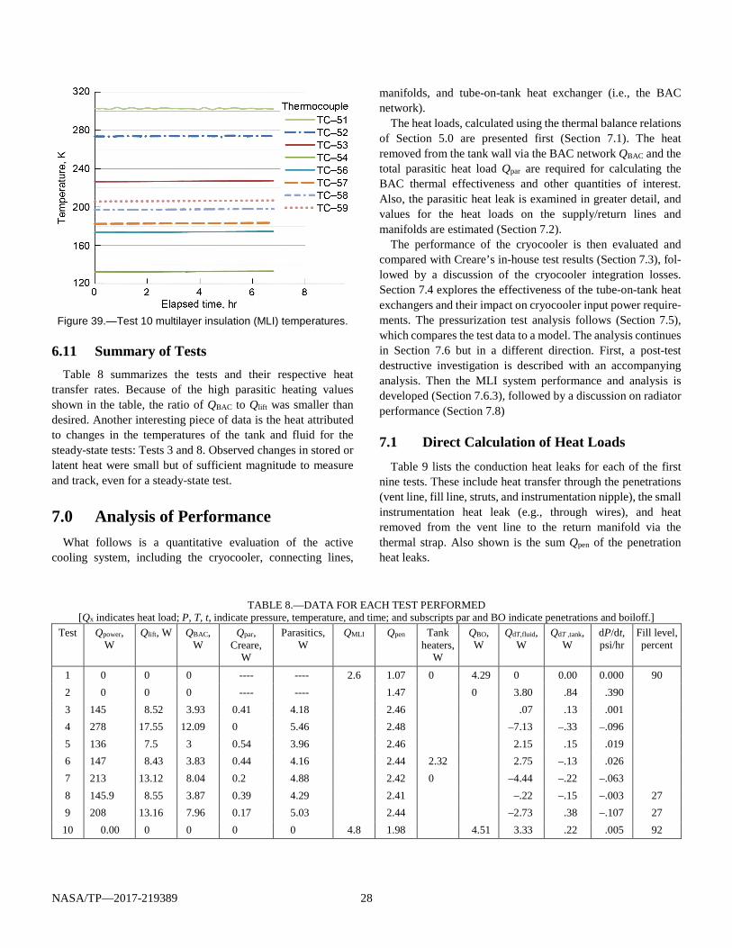
NASA/TP—2017-219389 28

Figure 39.—Test 10 multilayer insulation (MLI) temperatures.

6.11 Summary of Tests Table 8 summarizes the tests and their respective heat

transfer rates. Because of the high parasitic heating values shown in the table, the ratio of QBAC to Qlift was smaller than desired. Another interesting piece of data is the heat attributed to changes in the temperatures of the tank and fluid for the steady-state tests: Tests 3 and 8. Observed changes in stored or latent heat were small but of sufficient magnitude to measure and track, even for a steady-state test.

7.0 Analysis of Performance What follows is a quantitative evaluation of the active

cooling system, including the cryocooler, connecting lines,

manifolds, and tube-on-tank heat exchanger (i.e., the BAC network).

The heat loads, calculated using the thermal balance relations of Section 5.0 are presented first (Section 7.1). The heat removed from the tank wall via the BAC network QBAC and the total parasitic heat load Qpar are required for calculating the BAC thermal effectiveness and other quantities of interest. Also, the parasitic heat leak is examined in greater detail, and values for the heat loads on the supply/return lines and manifolds are estimated (Section 7.2).

The performance of the cryocooler is then evaluated and compared with Creare’s in-house test results (Section 7.3), fol-lowed by a discussion of the cryocooler integration losses. Section 7.4 explores the effectiveness of the tube-on-tank heat exchangers and their impact on cryocooler input power require-ments. The pressurization test analysis follows (Section 7.5), which compares the test data to a model. The analysis continues in Section 7.6 but in a different direction. First, a post-test destructive investigation is described with an accompanying analysis. Then the MLI system performance and analysis is developed (Section 7.6.3), followed by a discussion on radiator performance (Section 7.8)

7.1 Direct Calculation of Heat Loads Table 9 lists the conduction heat leaks for each of the first

nine tests. These include heat transfer through the penetrations (vent line, fill line, struts, and instrumentation nipple), the small instrumentation heat leak (e.g., through wires), and heat removed from the vent line to the return manifold via the thermal strap. Also shown is the sum Qpen of the penetration heat leaks.

TABLE 8.—DATA FOR EACH TEST PERFORMED [Qx indicates heat load; P, T, t, indicate pressure, temperature, and time; and subscripts par and BO indicate penetrations and boiloff.]

Test Qpower, W

Qlift, W QBAC, W

Qpar, Creare,

W

Parasitics, W

QMLI Qpen Tank heaters,

W

QBO, W

QdT,fluid, W

QdT ,tank, W

dP/dt, psi/hr

Fill level, percent

1 0 0 0 ---- ---- 2.6 1.07 0 4.29 0 0.00 0.000 90 2 0 0 0 ---- ---- 1.47 0 3.80 .84 .390 3 145 8.52 3.93 0.41 4.18 2.46 .07 .13 .001 4 278 17.55 12.09 0 5.46 2.48 –7.13 –.33 –.096 5 136 7.5 3 0.54 3.96 2.46 2.15 .15 .019 6 147 8.43 3.83 0.44 4.16 2.44 2.32 2.75 –.13 .026 7 213 13.12 8.04 0.2 4.88 2.42 0 –4.44 –.22 –.063 8 145.9 8.55 3.87 0.39 4.29 2.41 –.22 –.15 –.003 27 9 208 13.16 7.96 0.17 5.03 2.44 –2.73 .38 –.107 27 10 0.00 0 0 0 0 4.8 1.98 4.51 3.33 .22 .005 92

NASA/TP—2017-219389 29

TABLE 9.—CONDUCTION HEAT LEAKS, Q [Subscript pen indicates penetrations.]

Test number

Qvent, W

Qfill, W

Qstruts, W

Qnipple, W

Qpen, W

Qinst, W

Qstrap, W

1 0.71 0.49 0.38 0.06 1.64 0.04 –0.57 2 1.03 .48 .38 .06 1.95 .04 –.53 3 .95 .51 .40 .06 1.92 .03 .48 4 .95 .51 .40 .07 1.93 .03 .49 5 .97 .51 .40 .06 1.94 .03 .46 6 .95 .50 .39 1.91 .04 7 .94 .50 .39 1.90 .03 8 .94 .49 .39 1.89 .04 9 .96 .50 .40 1.92 .03

As discussed in Section 5.1.2, the heat Qwall absorbed by the

stainless steel tank wall is given by the temperature rise rates measured at various points around the tank (see Table 6). For most of the tests performed, this is a small correction to the total tank heat load Qtank, which is dominated by the heat absorbed by the contents (fluid and vapor) within the tank. The tank heat Qtank is consistent with expected results for the tests. In Test 2 (passive pressure rise), Qtank is slightly higher than in Test 1 (passive boiloff) because the vent line is no longer being cooled by the vent vapor. Tests 4, 7, and 9 have negative Qtank because more heat is being removed, which causes the tank pressure to decrease. In Test 3 (ZBO), QBAC is slightly less than in Test 2.

Table 10 compares the total heat load on the tank with the cryocooler lift. These numbers give an indication of how much cooling power must be applied to remove a given amount of heat from the tank. The total heat load thus defines the integration losses for each active test. For example, comparing Test 3 (ZBO) to Test 2 (passive pressure rise), Qtank falls from 4.6 W to practically zero. To accomplish this, 8.5 W of cooling power must be applied. Therefore, the Test 3 integration losses amount to around 4 W.

In Section 5.2 the authors reasoned that the heat leak to the tank through the MLI was nearly constant across the nine tests discussed. This argument was based largely on the fact that measured tank wall temperatures (the MLI cold boundary temperatures), as shown in Table 7, varied only slightly from test to test. For all but Test 1 (the passive boiloff test), it was impossible to calculate the MLI heat leak directly from the tank thermal balance, Equation (6). Thus, the authors assumed that for all tests, QMLI = QMLI, Test 1 = 2.62 W.

The cooling loop thermal balance in Equation (12) was used to determine the total parasitic heat load Qpar for each test in Table 11. The average is 4.2 W.

In Table 12, values of Qtank, Qcc, QBAC, and Qpar are provided with corresponding uncertainties, calculated as described in Section 5.4. As expected, the largest errors are seen in the

TABLE 10.—NEON MASS FLOW RATE; HEAT INTO THE CRYCOOLER (CC); TANK HEAT

Test number

Mass flow rate, m , g/s

Qcc, W

Qtank, W

1 0 0 4.29 2 0 0 4.61 3 1.70 8.51 .05 4 2.23 17.52 –7.42 5 1.64 7.48 2.22 6 1.70 8.42 2.83 7 1.99 13.10 –4.62 8 1.70 8.54 –.23 9 2.00 13.14 –3.08

TABLE 11.—COOLER LOOP HEAT LOADS, Q

[QBAC and Qpar are direct thermal balance results. BAC, par, and cc refer to broad-area cooling, parasitic, and cryocooler.]

Test number

Qcc, W

Qstrap, W

QBAC, W

Qpar, W

1 0.00 –0.57 0.00 0.57 2 .00 –.53 .00 .53 3 8.51 .48 4.52 3.51 4 17.52 .49 12.01 5.02 5 7.48 .46 2.37 4.65 6 8.42 4.06 3.90 7 13.10 9.17 3.47 8 8.54 4.77 3.31 9 13.14 7.65 5.03

Section 5.4. As expected, the largest errors are seen in the “downstream” quantities (refer to Figure 28) such as the parasitic heat leak. The MLI heat leak is QMLI = 2.62±0.54 W, the same for all tests. The uncertainties in Qpen and Qinstr are 0.46 W and 0.01 W, respectively; again, the same for all tests.

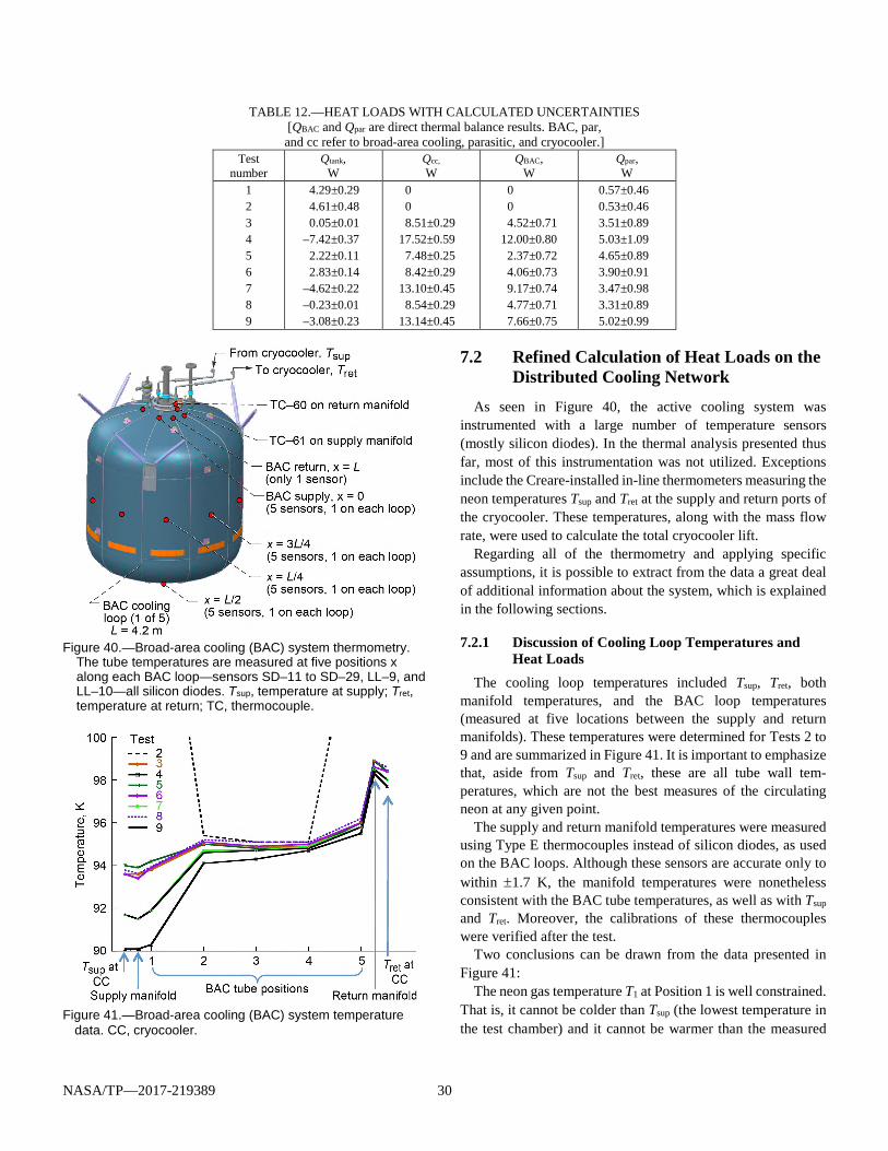
NASA/TP—2017-219389 30

TABLE 12.—HEAT LOADS WITH CALCULATED UNCERTAINTIES [QBAC and Qpar are direct thermal balance results. BAC, par, and cc refer to broad-area cooling, parasitic, and cryocooler.]

Test number

Qtank, W

Qcc,

W QBAC,

W Qpar, W

1 4.29±0.29 0 0 0.57±0.46 2 4.61±0.48 0 0 0.53±0.46 3 0.05±0.01 8.51±0.29 4.52±0.71 3.51±0.89 4 –7.42±0.37 17.52±0.59 12.00±0.80 5.03±1.09 5 2.22±0.11 7.48±0.25 2.37±0.72 4.65±0.89 6 2.83±0.14 8.42±0.29 4.06±0.73 3.90±0.91 7 –4.62±0.22 13.10±0.45 9.17±0.74 3.47±0.98 8 –0.23±0.01 8.54±0.29 4.77±0.71 3.31±0.89 9 –3.08±0.23 13.14±0.45 7.66±0.75 5.02±0.99

Figure 40.—Broad-area cooling (BAC) system thermometry.

The tube temperatures are measured at five positions x along each BAC loop—sensors SD–11 to SD–29, LL–9, and LL–10—all silicon diodes. Tsup, temperature at supply; Tret, temperature at return; TC, thermocouple.

Figure 41.—Broad-area cooling (BAC) system temperature

data. CC, cryocooler.

7.2 Refined Calculation of Heat Loads on the Distributed Cooling Network

As seen in Figure 40, the active cooling system was instrumented with a large number of temperature sensors (mostly silicon diodes). In the thermal analysis presented thus far, most of this instrumentation was not utilized. Exceptions include the Creare-installed in-line thermometers measuring the neon temperatures Tsup and Tret at the supply and return ports of the cryocooler. These temperatures, along with the mass flow rate, were used to calculate the total cryocooler lift.

Regarding all of the thermometry and applying specific assumptions, it is possible to extract from the data a great deal of additional information about the system, which is explained in the following sections.

7.2.1 Discussion of Cooling Loop Temperatures and Heat Loads

The cooling loop temperatures included Tsup, Tret, both manifold temperatures, and the BAC loop temperatures (measured at five locations between the supply and return manifolds). These temperatures were determined for Tests 2 to 9 and are summarized in Figure 41. It is important to emphasize that, aside from Tsup and Tret, these are all tube wall tem-peratures, which are not the best measures of the circulating neon at any given point.

The supply and return manifold temperatures were measured using Type E thermocouples instead of silicon diodes, as used on the BAC loops. Although these sensors are accurate only to within ±1.7 K, the manifold temperatures were nonetheless consistent with the BAC tube temperatures, as well as with Tsup and Tret. Moreover, the calibrations of these thermocouples were verified after the test.

Two conclusions can be drawn from the data presented in Figure 41:

The neon gas temperature T1 at Position 1 is well constrained. That is, it cannot be colder than Tsup (the lowest temperature in the test chamber) and it cannot be warmer than the measured

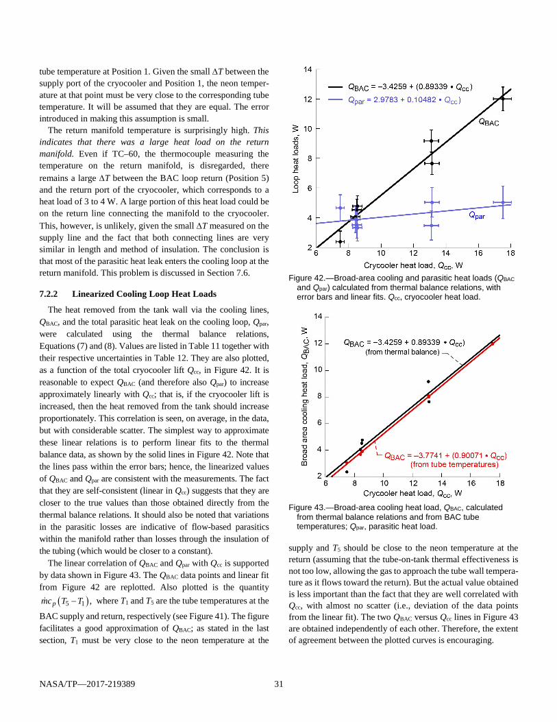
NASA/TP—2017-219389 31

tube temperature at Position 1. Given the small ∆T between the supply port of the cryocooler and Position 1, the neon temper-ature at that point must be very close to the corresponding tube temperature. It will be assumed that they are equal. The error introduced in making this assumption is small.

The return manifold temperature is surprisingly high. This indicates that there was a large heat load on the return manifold. Even if TC–60, the thermocouple measuring the temperature on the return manifold, is disregarded, there remains a large ∆T between the BAC loop return (Position 5) and the return port of the cryocooler, which corresponds to a heat load of 3 to 4 W. A large portion of this heat load could be on the return line connecting the manifold to the cryocooler. This, however, is unlikely, given the small ∆T measured on the supply line and the fact that both connecting lines are very similar in length and method of insulation. The conclusion is that most of the parasitic heat leak enters the cooling loop at the return manifold. This problem is discussed in Section 7.6.

7.2.2 Linearized Cooling Loop Heat Loads

The heat removed from the tank wall via the cooling lines, QBAC, and the total parasitic heat leak on the cooling loop, Qpar, were calculated using the thermal balance relations, Equations (7) and (8). Values are listed in Table 11 together with their respective uncertainties in Table 12. They are also plotted, as a function of the total cryocooler lift Qcc, in Figure 42. It is reasonable to expect QBAC (and therefore also Qpar) to increase approximately linearly with Qcc; that is, if the cryocooler lift is increased, then the heat removed from the tank should increase proportionately. This correlation is seen, on average, in the data, but with considerable scatter. The simplest way to approximate these linear relations is to perform linear fits to the thermal balance data, as shown by the solid lines in Figure 42. Note that the lines pass within the error bars; hence, the linearized values of QBAC and Qpar are consistent with the measurements. The fact that they are self-consistent (linear in Qcc) suggests that they are closer to the true values than those obtained directly from the thermal balance relations. It should also be noted that variations in the parasitic losses are indicative of flow-based parasitics within the manifold rather than losses through the insulation of the tubing (which would be closer to a constant).

The linear correlation of QBAC and Qpar with Qcc is supported by data shown in Figure 43. The QBAC data points and linear fit from Figure 42 are replotted. Also plotted is the quantity

( )5 1 ,pmc T T− where T1 and T5 are the tube temperatures at the

BAC supply and return, respectively (see Figure 41). The figure facilitates a good approximation of QBAC; as stated in the last section, T1 must be very close to the neon temperature at the

Figure 42.—Broad-area cooling and parasitic heat loads (QBAC

and Qpar) calculated from thermal balance relations, with error bars and linear fits. Qcc, cryocooler heat load.

Figure 43.—Broad-area cooling heat load, QBAC, calculated

from thermal balance relations and from BAC tube temperatures; Qpar, parasitic heat load.

supply and T5 should be close to the neon temperature at the return (assuming that the tube-on-tank thermal effectiveness is not too low, allowing the gas to approach the tube wall tempera-ture as it flows toward the return). But the actual value obtained is less important than the fact that they are well correlated with Qcc, with almost no scatter (i.e., deviation of the data points from the linear fit). The two QBAC versus Qcc lines in Figure 43 are obtained independently of each other. Therefore, the extent of agreement between the plotted curves is encouraging.

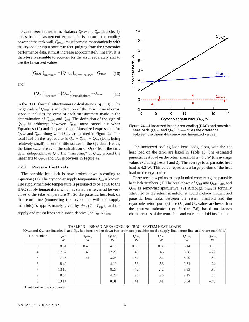
NASA/TP—2017-219389 32

Scatter seen in the thermal-balance QBAC and Qpar data clearly arises from measurement error. This is because the cooling power at the tank wall, QBAC, must increase monotonically with the cryocooler input power; in fact, judging from the cryocooler performance data, it must increase approximately linearly. It is therefore reasonable to account for the error separately and to use the linearized values,

( ) ( )BAC BAC errorlinearized thermal balanceQ Q Q= − (10)

and

( ) ( )par par errorlinearized thermal balanceQ Q Q= − (11)

in the BAC thermal effectiveness calculations (Eq. (13)). The magnitude of Qerror is an indication of the measurement error, since it includes the error of each measurement made in the determination of QBAC and Qpar. The definition of the sign of Qerror is arbitrary; however, Qerror must cancel out when Equations (10) and (11) are added. Linearized expressions for QBAC and Qpar, along with Qerror, are plotted in Figure 44. The total load on the cryocooler is Qcc ~ QBAC + Qpar (Qstrap being relatively small). There is little scatter in the Qcc data. Hence, the large Qerror arises in the calculation of QBAC from the tank data, independent of Qcc. The “mirroring” of Qerror around the linear fits to QBAC and Qpar is obvious in Figure 42.

7.2.3 Parasitic Heat Leaks The parasitic heat leak is now broken down according to

Equation (11). The cryocooler supply temperature Tsup is known. The supply manifold temperature is presumed to be equal to the BAC supply temperature, which as stated earlier, must be very close to the tube temperature T1. So the parasitic heat leak on the return line (connecting the cryocooler with the supply manifold) is approximately given by ( )1 suppmc T T− , and the

supply and return lines are almost identical, so Qret ≈ Qsup.

Figure 44.—Linearized broad-area cooling (BAC) and parasitic

heat loads (QBAC and Qpar); Qerror gives the difference between the thermal-balance and linearized values.

The linearized cooling loop heat loads, along with the net

heat load on the tank, are listed in Table 13. The estimated parasitic heat load on the return manifold is ~3.3 W (the average value, excluding Tests 1 and 2). The average total parasitic heat load is 4.2 W. This value represents a large portion of the heat load on the cryocooler.

There are a few points to keep in mind concerning the parasitic heat leak numbers. (1) The breakdown of Qpar into Qsup, Qret, and Qman is somewhat speculative. (2) Although Qman is formally attributed to the return manifold, it could include unidentified parasitic heat leaks between the return manifold and the cryocooler return port. (3) The Qsup and Qret values are lower than the posttest estimates (see Section 7.6) based on known characteristics of the return line and valve manifold insulation.

TABLE 13.—BROAD-AREA COOLING (BAC) SYSTEM HEAT LOADS

[QBAC and Qpar are linearized, and Qpar has been broken down into estimated parasitics on the supply line, return line, and return manifold.] Test number Qcc,a

W Qstrap,

W QBAC,

W Qsup, W

Qret, W

Qman, W

Qerror, W

3 8.51 0.48 4.18 0.36 0.36 3.14 0.35 4 17.52 .49 12.23 .46 .46 3.88 –.22 5 7.48 .46 3.26 .34 .34 3.09 –.89 6 8.42 4.10 .53 .53 2.81 –.04 7 13.10 8.28 .42 .42 3.53 .90 8 8.54 4.20 .36 .36 3.17 .56 9 13.14 8.31 .41 .41 3.54 –.66

aHeat load on the cryocooler.

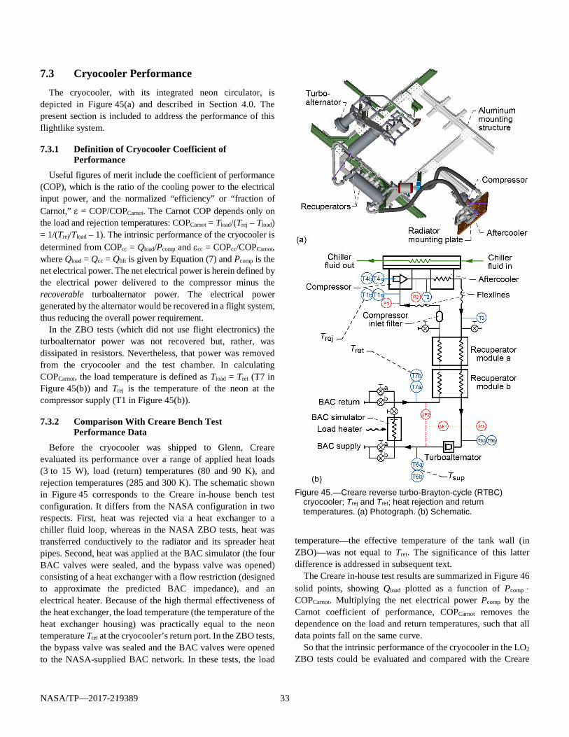
NASA/TP—2017-219389 33

7.3 Cryocooler Performance The cryocooler, with its integrated neon circulator, is

depicted in Figure 45(a) and described in Section 4.0. The present section is included to address the performance of this flightlike system.

7.3.1 Definition of Cryocooler Coefficient of Performance

Useful figures of merit include the coefficient of performance (COP), which is the ratio of the cooling power to the electrical input power, and the normalized “efficiency” or “fraction of Carnot,” ε = COP/COPCarnot. The Carnot COP depends only on the load and rejection temperatures: COPCarnot = Tload/(Trej – Tload) = 1/(Trej/Tload – 1). The intrinsic performance of the cryocooler is determined from COPcc = Qload/Pcomp and εcc = COPcc/COPCarnot, where Qload = Qcc = Qlift is given by Equation (7) and Pcomp is the net electrical power. The net electrical power is herein defined by the electrical power delivered to the compressor minus the recoverable turboalternator power. The electrical power generated by the alternator would be recovered in a flight system, thus reducing the overall power requirement.

In the ZBO tests (which did not use flight electronics) the turboalternator power was not recovered but, rather, was dissipated in resistors. Nevertheless, that power was removed from the cryocooler and the test chamber. In calculating COPCarnot, the load temperature is defined as Tload = Tret (T7 in Figure 45(b)) and Trej is the temperature of the neon at the compressor supply (T1 in Figure 45(b)).

7.3.2 Comparison With Creare Bench Test Performance Data

Before the cryocooler was shipped to Glenn, Creare evaluated its performance over a range of applied heat loads (3 to 15 W), load (return) temperatures (80 and 90 K), and rejection temperatures (285 and 300 K). The schematic shown in Figure 45 corresponds to the Creare in-house bench test configuration. It differs from the NASA configuration in two respects. First, heat was rejected via a heat exchanger to a chiller fluid loop, whereas in the NASA ZBO tests, heat was transferred conductively to the radiator and its spreader heat pipes. Second, heat was applied at the BAC simulator (the four BAC valves were sealed, and the bypass valve was opened) consisting of a heat exchanger with a flow restriction (designed to approximate the predicted BAC impedance), and an electrical heater. Because of the high thermal effectiveness of the heat exchanger, the load temperature (the temperature of the heat exchanger housing) was practically equal to the neon temperature Tret at the cryocooler’s return port. In the ZBO tests, the bypass valve was sealed and the BAC valves were opened to the NASA-supplied BAC network. In these tests, the load

Figure 45.—Creare reverse turbo-Brayton-cycle (RTBC)

cryocooler; Trej and Tret; heat rejection and return temperatures. (a) Photograph. (b) Schematic.

temperature—the effective temperature of the tank wall (in ZBO)—was not equal to Tret. The significance of this latter difference is addressed in subsequent text.

The Creare in-house test results are summarized in Figure 46 solid points, showing Qload plotted as a function of Pcomp ⋅ COPCarnot. Multiplying the net electrical power Pcomp by the Carnot coefficient of performance, COPCarnot removes the dependence on the load and return temperatures, such that all data points fall on the same curve.

So that the intrinsic performance of the cryocooler in the LO2 ZBO tests could be evaluated and compared with the Creare

NASA/TP—2017-219389 34

in-house measurements, Tret (as opposed to the effective tank wall temperature) was used to calculate COPCarnot. In the LO2 ZBO test, Tret ~ 98 K (compared with 80 and 90 K in the Creare tests), Trej ~ 280 K (compared with 285 and 300 K in Creare tests), and Qload = Qcc varied from ~8 W to nearly 18 W (compared with 3 to 15 W in the Creare tests). The results are plotted in Figure 46, and they all fall on the same line as the Creare in-house data points. Thus, the ZBO test data were consistent with the Creare bench test, and there was no measureable change in performance of the cryocooler over the course of ZBO testing.

7.3.3 Parasitics and Useful Refrigeration A portion of the cryocooler’s refrigeration capacity must be

used to overcome integration losses—parasitic heat leaks and heat exchanger ineffectiveness. Figure 47 demonstrates the truth of this statement. The total refrigeration, or cooling power, Qcc, is plotted versus Pcomp, but this includes the parasitic heat load Qpar. Also plotted is the useful refrigeration Quseful = Qcc – Qpar = QBAC + Qstrap. At the low-power end, about half of the available refrigeration is used to compensate for the parasitic heat leaks. This ratio decreases with increasing power. Comparing points of equal refrigeration (say, 8 W) shows that a penalty of 50 to 60 W of electrical power is incurred because of high integration losses.

7.3.4 System Coefficient of Performance Appropriate figures of merit for the active cooling system

(not just the cryocooler) are the system coefficient of performance COPsys = Quseful/Pcomp and the corresponding fraction of Carnot efficiency εsys = COPsys/COPCarnot. The latter is plotted in Figure 48, along with the bare cryocooler fraction of Carnot efficiency εcc for comparison. In calculating εsys, the load temperature is identified as the effective wall temperature (calculated in the following section), which is approximately equal to the area-weighted average tank wall temperature. This temperature is ~96.5 K, which is colder than the return temperature. The COP and fraction of Carnot increases with increasing power, and εcc ranges from ~10 to 12 percent, which are respectable numbers for a flightlike cryocooler of this size (Ref. 26), whereas εsys is only ~5 to 9 percent. Also shown in Figure 48 is the system fraction of Carnot efficiency that would result if the anomalously high heat load Qman on the return manifold was eliminated. The curve is shifted to the left by Qman ~ 3 W. It approaches εcc as the power increases, and it reaches a reasonably high value of ~11 percent at Qcc = 15 W. The two curves do not coincide because there remains a total parasitic loss/load of ~1 W on the supply and return lines.

Figure 46.—Cryocooler performance data for zero boiloff

(ZBO) and Creare tests.

Figure 47.—Total cryocooler (subscript cc) refrigeration and

useful refrigeration: Quseful = Qcc – Qpar; BAC, broad-area cooling.

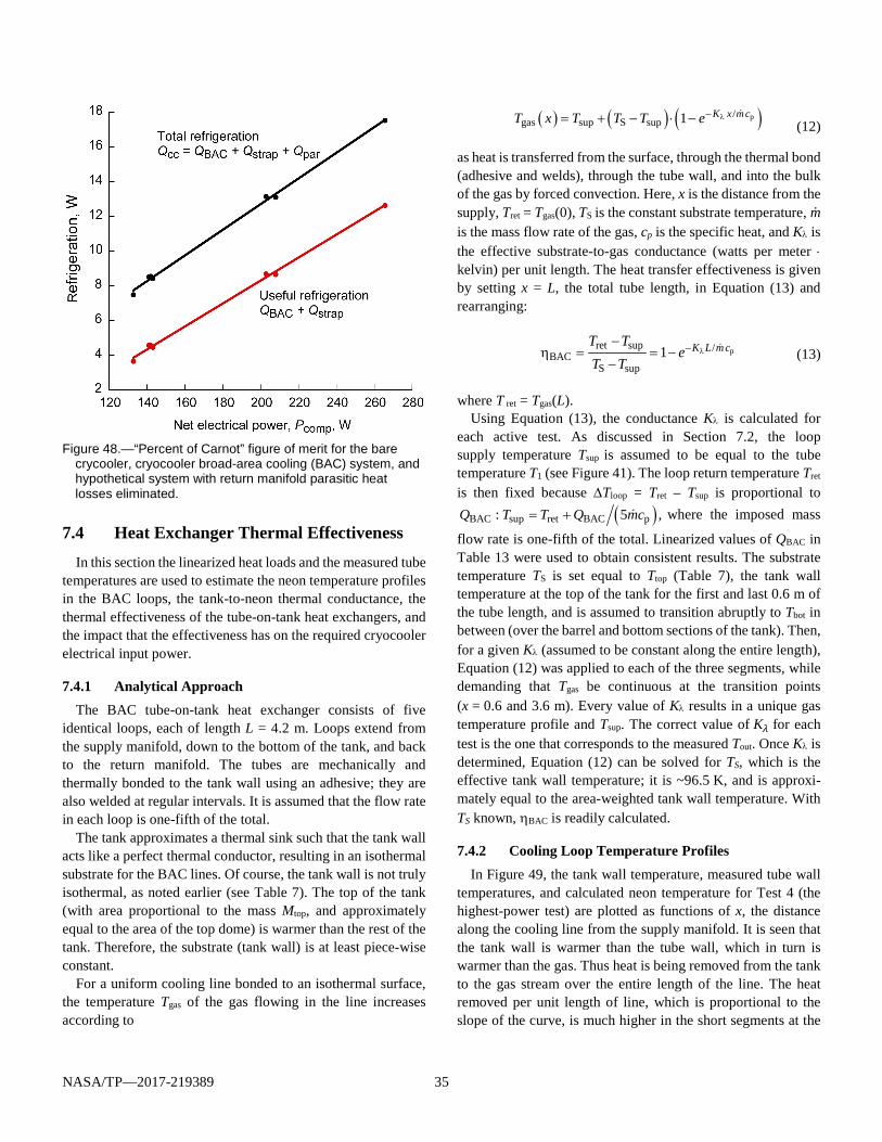
NASA/TP—2017-219389 35

Figure 48.—“Percent of Carnot” figure of merit for the bare

crycooler, cryocooler broad-area cooling (BAC) system, and hypothetical system with return manifold parasitic heat losses eliminated.

7.4 Heat Exchanger Thermal Effectiveness In this section the linearized heat loads and the measured tube

temperatures are used to estimate the neon temperature profiles in the BAC loops, the tank-to-neon thermal conductance, the thermal effectiveness of the tube-on-tank heat exchangers, and the impact that the effectiveness has on the required cryocooler electrical input power.

7.4.1 Analytical Approach The BAC tube-on-tank heat exchanger consists of five

identical loops, each of length L = 4.2 m. Loops extend from the supply manifold, down to the bottom of the tank, and back to the return manifold. The tubes are mechanically and thermally bonded to the tank wall using an adhesive; they are also welded at regular intervals. It is assumed that the flow rate in each loop is one-fifth of the total.

The tank approximates a thermal sink such that the tank wall acts like a perfect thermal conductor, resulting in an isothermal substrate for the BAC lines. Of course, the tank wall is not truly isothermal, as noted earlier (see Table 7). The top of the tank (with area proportional to the mass Mtop, and approximately equal to the area of the top dome) is warmer than the rest of the tank. Therefore, the substrate (tank wall) is at least piece-wise constant.

For a uniform cooling line bonded to an isothermal surface, the temperature Tgas of the gas flowing in the line increases according to

( ) ( ) ( )p/gas sup S sup 1 K x mcT x T T T e λ−= + − ⋅ − (12)

as heat is transferred from the surface, through the thermal bond (adhesive and welds), through the tube wall, and into the bulk of the gas by forced convection. Here, x is the distance from the supply, Tret = Tgas(0), TS is the constant substrate temperature, m is the mass flow rate of the gas, cp is the specific heat, and Kλ is the effective substrate-to-gas conductance (watts per meter ⋅ kelvin) per unit length. The heat transfer effectiveness is given by setting x = L, the total tube length, in Equation (13) and rearranging:

pret sup /BAC

S sup1 K L m cT T

eT T

λ−−η = = −

− (13)

where T ret = Tgas(L). Using Equation (13), the conductance Kλ is calculated for

each active test. As discussed in Section 7.2, the loop supply temperature Tsup is assumed to be equal to the tube temperature T1 (see Figure 41). The loop return temperature Tret is then fixed because ∆Tloop = Tret – Tsup is proportional to

( )BAC sup ret BAC p: 5 ,Q T T Q mc= + where the imposed mass

flow rate is one-fifth of the total. Linearized values of QBAC in Table 13 were used to obtain consistent results. The substrate temperature TS is set equal to Ttop (Table 7), the tank wall temperature at the top of the tank for the first and last 0.6 m of the tube length, and is assumed to transition abruptly to Tbot in between (over the barrel and bottom sections of the tank). Then, for a given Kλ (assumed to be constant along the entire length), Equation (12) was applied to each of the three segments, while demanding that Tgas be continuous at the transition points (x = 0.6 and 3.6 m). Every value of Kλ results in a unique gas temperature profile and Tsup. The correct value of K𝜆𝜆 for each test is the one that corresponds to the measured Tout. Once Kλ is determined, Equation (12) can be solved for TS, which is the effective tank wall temperature; it is ~96.5 K, and is approxi-mately equal to the area-weighted tank wall temperature. With TS known, ηBAC is readily calculated.

7.4.2 Cooling Loop Temperature Profiles In Figure 49, the tank wall temperature, measured tube wall

temperatures, and calculated neon temperature for Test 4 (the highest-power test) are plotted as functions of x, the distance along the cooling line from the supply manifold. It is seen that the tank wall is warmer than the tube wall, which in turn is warmer than the gas. Thus heat is being removed from the tank to the gas stream over the entire length of the line. The heat removed per unit length of line, which is proportional to the slope of the curve, is much higher in the short segments at the

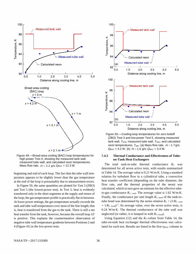
NASA/TP—2017-219389 36

Figure 49.—Broad-area cooling (BAC) loop temperatures for

high-power Test 4, showing the measured tank wall, measured tube wall, and calculated neon temperatures. Mass flow rate, = 2.2 g/s;m QBAC = 12.3 W.

beginning and end of each loop. The fact that the tube wall tem-perature appears to be slightly lower than the gas temperature at the end of the loop is presumably due to measurement errors.

In Figure 50, the same quantities are plotted for Test 3 (ZBO) and Test 5 (the lowest-power test). In Test 3, heat is evidently transferred only in the short segments at the supply and return of the loop; the gas temperature profile is practically flat in between. At lower power settings, the gas temperature actually exceeds the tank and tube wall temperatures over most of the line length; that is, heat is transferred from the gas to the tank. There is still a net heat transfer from the tank, however, because the overall loop ∆T is positive. This explains the counterintuitive observation of negative tube wall temperature gradients between Positions 2 and 4 (Figure 41) in the low-power tests.

Figure 50.—Cooling-loop temperatures for zero boiloff

(ZBO) Test 3 and low-power Test 5, showing measured tank wall, Ttank; measured tube wall, Ttube; and calculated neon temperatures, Tgas. (a) Mass flow rate, = 1.7g/s;m QBAC = 4.2 W. (b) = 1.6 g/s;m QBAC = 3.3 W.

7.4.3 Thermal Conductance and Effectiveness of Tube-on-Tank Heat Exchangers

The total tank-to-tube thermal conductance Kλ was determined for all seven active tests, with results summarized in Table 14. The average value is 0.21 W/m⋅K. Using a standard relation for turbulent flow in a cylindrical tube, a convective heat transfer coefficient (depending on the tube diameter, the flow rate, and the thermal properties of the neon) was calculated, which in turn gave an estimate for the effective tube-to-gas conductance Kλ, cond. The average value is 1.62 W/m⋅K. Finally, the conductance per unit length Kλ, bond of the tank-to-tube bond was determined by the series relation Kλ = (1/Kλ, cond + 1/Kλ, bond)–1. Its average value, over the seven active tests, is 0.24 W/m⋅K. The thermal conductance of the tube wall was neglected (or rather, it is lumped in with Kλ, bond).

Using Equation (12) and the Kλ-values from Table 14, the tube-on-tank heat exchanger thermal effectiveness was calcu-lated for each test. Results are listed in the first ηBAC column in

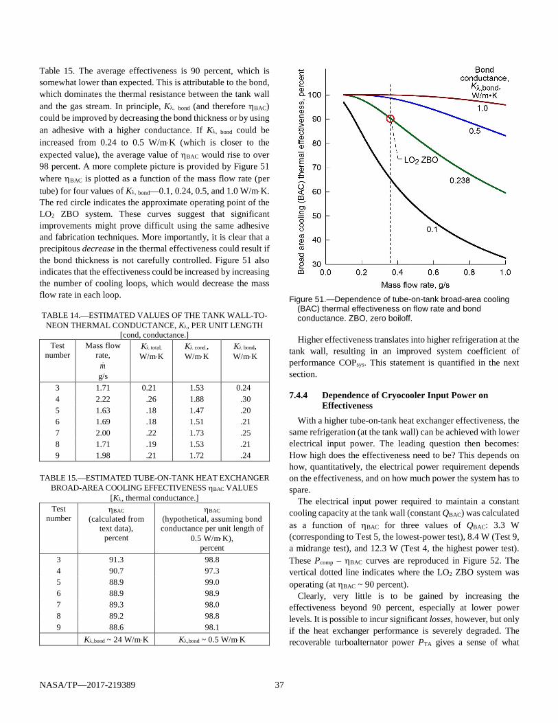
NASA/TP—2017-219389 37

Table 15. The average effectiveness is 90 percent, which is somewhat lower than expected. This is attributable to the bond, which dominates the thermal resistance between the tank wall and the gas stream. In principle, Kλ, bond (and therefore ηBAC) could be improved by decreasing the bond thickness or by using an adhesive with a higher conductance. If Kλ, bond could be increased from 0.24 to 0.5 W/m⋅K (which is closer to the expected value), the average value of ηBAC would rise to over 98 percent. A more complete picture is provided by Figure 51 where ηBAC is plotted as a function of the mass flow rate (per tube) for four values of Kλ, bond—0.1, 0.24, 0.5, and 1.0 W/m⋅K. The red circle indicates the approximate operating point of the LO2 ZBO system. These curves suggest that significant improvements might prove difficult using the same adhesive and fabrication techniques. More importantly, it is clear that a precipitous decrease in the thermal effectiveness could result if the bond thickness is not carefully controlled. Figure 51 also indicates that the effectiveness could be increased by increasing the number of cooling loops, which would decrease the mass flow rate in each loop. TABLE 14.—ESTIMATED VALUES OF THE TANK WALL-TO-

NEON THERMAL CONDUCTANCE, Kλ, PER UNIT LENGTH [cond, conductance.]

Test number

Mass flow rate,

m g/s

Kλ total,

W/m⋅K Kλ cond., W/m⋅K

Kλ bond, W/m⋅K

3 1.71 0.21 1.53 0.24 4 2.22 .26 1.88 .30 5 1.63 .18 1.47 .20 6 1.69 .18 1.51 .21 7 2.00 .22 1.73 .25 8 1.71 .19 1.53 .21 9 1.98 .21 1.72 .24

TABLE 15.—ESTIMATED TUBE-ON-TANK HEAT EXCHANGER

BROAD-AREA COOLING EFFECTIVENESS ηBAC VALUES [Kλ, thermal conductance.]

Test number

ηBAC (calculated from

text data), percent

ηBAC (hypothetical, assuming bond conductance per unit length of

0.5 W/m⋅K), percent

3 91.3 98.8 4 90.7 97.3 5 88.9 99.0 6 88.9 98.9 7 89.3 98.0 8 89.2 98.8 9 88.6 98.1 Kλ,bond ~ 24 W/m⋅K Kλ,bond ~ 0.5 W/m⋅K

Figure 51.—Dependence of tube-on-tank broad-area cooling

(BAC) thermal effectiveness on flow rate and bond conductance. ZBO, zero boiloff. Higher effectiveness translates into higher refrigeration at the

tank wall, resulting in an improved system coefficient of performance COPsys. This statement is quantified in the next section.

7.4.4 Dependence of Cryocooler Input Power on Effectiveness

With a higher tube-on-tank heat exchanger effectiveness, the same refrigeration (at the tank wall) can be achieved with lower electrical input power. The leading question then becomes: How high does the effectiveness need to be? This depends on how, quantitatively, the electrical power requirement depends on the effectiveness, and on how much power the system has to spare.

The electrical input power required to maintain a constant cooling capacity at the tank wall (constant QBAC) was calculated as a function of ηBAC for three values of QBAC: 3.3 W (corresponding to Test 5, the lowest-power test), 8.4 W (Test 9, a midrange test), and 12.3 W (Test 4, the highest power test). These Pcomp – ηBAC curves are reproduced in Figure 52. The vertical dotted line indicates where the LO2 ZBO system was operating (at ηBAC ~ 90 percent).

Clearly, very little is to be gained by increasing the effectiveness beyond 90 percent, especially at lower power levels. It is possible to incur significant losses, however, but only if the heat exchanger performance is severely degraded. The recoverable turboalternator power PTA gives a sense of what

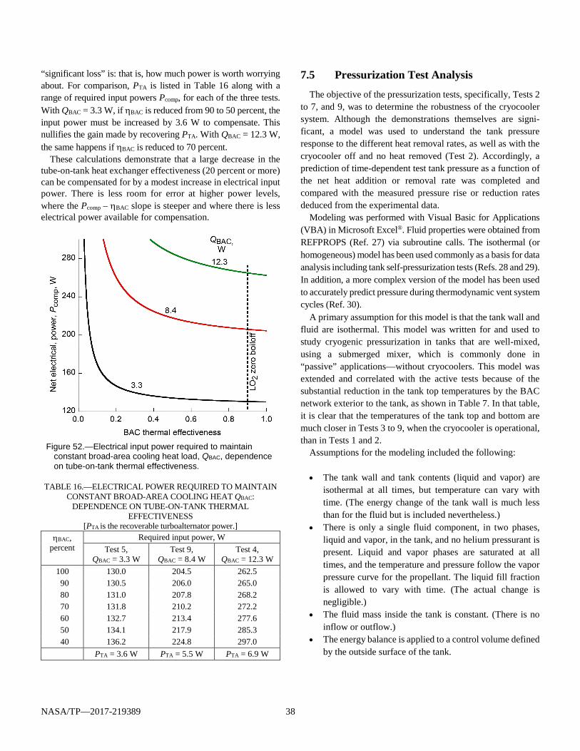
NASA/TP—2017-219389 38

“significant loss” is: that is, how much power is worth worrying about. For comparison, PTA is listed in Table 16 along with a range of required input powers Pcomp, for each of the three tests. With QBAC = 3.3 W, if ηBAC is reduced from 90 to 50 percent, the input power must be increased by 3.6 W to compensate. This nullifies the gain made by recovering PTA. With QBAC = 12.3 W, the same happens if ηBAC is reduced to 70 percent.

These calculations demonstrate that a large decrease in the tube-on-tank heat exchanger effectiveness (20 percent or more) can be compensated for by a modest increase in electrical input power. There is less room for error at higher power levels, where the Pcomp – ηBAC slope is steeper and where there is less electrical power available for compensation.

Figure 52.—Electrical input power required to maintain

constant broad-area cooling heat load, QBAC, dependence on tube-on-tank thermal effectiveness.

TABLE 16.—ELECTRICAL POWER REQUIRED TO MAINTAIN

CONSTANT BROAD-AREA COOLING HEAT QBAC: DEPENDENCE ON TUBE-ON-TANK THERMAL

EFFECTIVENESS [PTA is the recoverable turboalternator power.]

ηBAC, percent

Required input power, W Test 5,

QBAC = 3.3 W Test 9,

QBAC = 8.4 W Test 4,

QBAC = 12.3 W 100 130.0 204.5 262.5

90 130.5 206.0 265.0 80 131.0 207.8 268.2 70 131.8 210.2 272.2 60 132.7 213.4 277.6 50 134.1 217.9 285.3 40 136.2 224.8 297.0

PTA = 3.6 W PTA = 5.5 W PTA = 6.9 W

7.5 Pressurization Test Analysis

The objective of the pressurization tests, specifically, Tests 2 to 7, and 9, was to determine the robustness of the cryocooler system. Although the demonstrations themselves are signi-ficant, a model was used to understand the tank pressure response to the different heat removal rates, as well as with the cryocooler off and no heat removed (Test 2). Accordingly, a prediction of time-dependent test tank pressure as a function of the net heat addition or removal rate was completed and compared with the measured pressure rise or reduction rates deduced from the experimental data.

Modeling was performed with Visual Basic for Applications (VBA) in Microsoft Excel®. Fluid properties were obtained from REFPROPS (Ref. 27) via subroutine calls. The isothermal (or homogeneous) model has been used commonly as a basis for data analysis including tank self-pressurization tests (Refs. 28 and 29). In addition, a more complex version of the model has been used to accurately predict pressure during thermodynamic vent system cycles (Ref. 30).

A primary assumption for this model is that the tank wall and fluid are isothermal. This model was written for and used to study cryogenic pressurization in tanks that are well-mixed, using a submerged mixer, which is commonly done in “passive” applications—without cryocoolers. This model was extended and correlated with the active tests because of the substantial reduction in the tank top temperatures by the BAC network exterior to the tank, as shown in Table 7. In that table, it is clear that the temperatures of the tank top and bottom are much closer in Tests 3 to 9, when the cryocooler is operational, than in Tests 1 and 2.

Assumptions for the modeling included the following: • The tank wall and tank contents (liquid and vapor) are

isothermal at all times, but temperature can vary with time. (The energy change of the tank wall is much less than for the fluid but is included nevertheless.)

• There is only a single fluid component, in two phases, liquid and vapor, in the tank, and no helium pressurant is present. Liquid and vapor phases are saturated at all times, and the temperature and pressure follow the vapor pressure curve for the propellant. The liquid fill fraction is allowed to vary with time. (The actual change is negligible.)

• The fluid mass inside the tank is constant. (There is no inflow or outflow.)

• The energy balance is applied to a control volume defined by the outside surface of the tank.

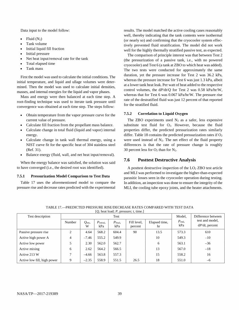
NASA/TP—2017-219389 39

Data input to the model follow:

• Fluid (N2) • Tank volume • Initial liquid fill fraction • Initial pressure • Net heat input/removal rate for the tank • Total elapsed time • Tank mass

First the model was used to calculate the initial conditions. The initial temperature, and liquid and ullage volumes were deter-mined. Then the model was used to calculate initial densities, masses, and internal energies for the liquid and vapor phases.

Mass and energy were then balanced at each time step. A root-finding technique was used to iterate tank pressure until convergence was obtained at each time step. The steps follow:

• Obtain temperature from the vapor pressure curve for the current value of pressure.

• Calculate fill fraction from the propellant mass balance. • Calculate change in total fluid (liquid and vapor) internal

energy. • Calculate change in tank wall thermal energy, using a

NIST curve fit for the specific heat of 304 stainless steel (Ref. 31).

• Balance energy (fluid, wall, and net heat input/removal).

When the energy balance was satisfied, the solution was said to have converged (i.e., the desired root was identified).

7.5.1 Pressurization Model Comparison to Test Data Table 17 uses the aforementioned model to compare the

pressure rise and decrease rates predicted with the experimental

results. The model matched the active cooling cases reasonably well, thereby indicating that the tank contents were isothermal (or nearly so) and confirming that the cryocooler system effec-tively prevented fluid stratification. The model did not work well for the highly thermally stratified passive test, as expected.

The comparison of principle interest was that between Test 2 (the pressurization of a passive tank, i.e., with no powered cryocooler) and Test 6 (a tank at ZBO to which heat was added). The two tests were conducted for approximately the same duration, yet the pressure increase for Test 2 was 36.2 kPa, whereas the pressure increase for Test 6 was just 1.3 kPa, albeit at a lower tank heat leak. Per watt of heat added to the respective control volumes, the dP/dt/Q for Test 2 was 0.58 kPa/hr/W, whereas that for Test 6 was 0.067 kPa/hr/W. The pressure rise rate of the destratified fluid was just 12 percent of that reported for the stratified fluid.

7.5.2 Correlation to Liquid Oxygen The ZBO experiments used N2 as a safer, less expensive

substitute test fluid for O2. However, because the fluid properties differ, the predicted pressurization rates similarly differ. Table 18 contains the predicted pressurization rates if O2 were used instead of N2. The net effect of the fluid property differences is that the rate of pressure change is roughly 30 percent less for O2 than for N2.

7.6 Posttest Destructive Analysis A posttest destructive inspection of the LO2 ZBO test article

and MLI was performed to investigate the higher-than-expected parasitic losses seen in the cryocooler operation during testing. In addition, an inspection was done to ensure the integrity of the MLI, the cooling tube epoxy joints, and the heater attachments.

TABLE 17.—PREDICTED PRESSURE RISE/DECREASE RATES COMPARED WITH TEST DATA [Q, heat load; P, pressure; t, time.]

Test description Test Model, Pend, kPa

Difference between test and model, dP/dt, percent

Number Qnet, W

Pinitial, kPa

Pfinal, kPa

Fill level, percent

Elapsed time, hr

Passive pressure rise 2 4.64 568.2 604.4 90 13.5 573.3 610 Active high power A 4 –7.46 555.2 549.9 10 549.3 –10 Active low power 5 2.30 562.0 562.7 6 563.1 –36 Active mixing 6 2.62 564.2 566.5 13 567.0 –18 Active 213 W 7 –4.66 563.8 557.3 15 558.2 16 Active low fill, high power 9 –2.35 558.9 551.5 26.5 18 551.0 –6

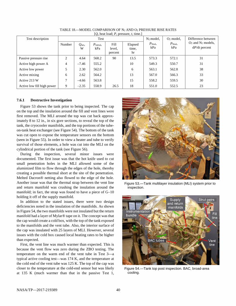
NASA/TP—2017-219389 40

TABLE 18.—MODEL COMPARISON OF N2 AND O2 PRESSURE RISE RATES [Q, heat load; P, pressure, t, time.]

Test description Test N2 model, Pfinal, kPa

O2 model, Pfinal, kPa

Difference between O2 and N2 models,

dP/dt percent Number Qnet,

W Pinitial, kPa

Fill level,

percent

Elapsed time,

hr

Passive pressure rise 2 4.64 568.2 90 13.5 573.3 572.1 31 Active high power A 4 –7.46 555.2 10 549.3 550.7 31 Active low power 5 2.30 562.0 6 563.1 562.8 38 Active mixing 6 2.62 564.2 13 567.0 566.3 33 Active 213 W 7 –4.66 563.8 15 558.2 559.5 30 Active low fill high power 9 –2.35 558.9 26.5 18 551.0 552.5 23

7.6.1 Destructive Investigation Figure 53 shows the tank prior to being inspected. The cap

on the top and the insulation around the fill and vent lines were first removed. The MLI around the top was cut back approx-imately 8 to 12 in., in six gore sections, to reveal the top of the tank, the cryocooler manifolds, and the top portions of the tube-on-tank heat exchanger (see Figure 54). The bottom of the tank was cut open to expose the temperature sensors on the bottom (seen in Figure 55). In order to view a heater and tube to verify survival of those elements, a hole was cut into the MLI on the cylindrical portion of the tank (see Figure 56).

During the inspection, several minor issues were documented. The first issue was that the hot knife used to cut small penetration holes in the MLI allowed some of the aluminized film to flow through the edges of the hole, thereby creating a possible thermal short at the site of the penetration. Melted Dacron® netting also flowed to the edge of the hole. Another issue was that the thermal strap between the vent line and return manifold was crushing the insulation around the manifold; in fact, the strap was found to have a piece of G–10 holding it off of the supply manifold.

In addition to the stated issues, there were two design deficiencies noted in the insulation of the manifolds. As shown in Figure 54, the two manifolds were not insulated but the return manifold had a layer of Mylar® tape on it. The concept was that the cap would create a cold box, with the top of the tank exposed to the manifolds and the vent tube. Also, the interior surface of the cap was insulated with 25 layers of MLI. However, several issues with the cold box caused local heating rates to be higher than expected.

First, the vent line was much warmer than expected. This is because the vent flow was zero during the ZBO testing. The temperature on the warm end of the vent tube in Test 3—a typical active cooling test—was 174 K, and the temperature at the cold end of the vent tube was 125 K. The top of the cap was closer to the temperature at the cold-end sensor but was likely at 135 K (much warmer than that in the passive Test 1,

Figure 53.—Tank multilayer insulation (MLI) system prior to

inspection.

Figure 54.—Tank top post inspection. BAC, broad-area

cooling.

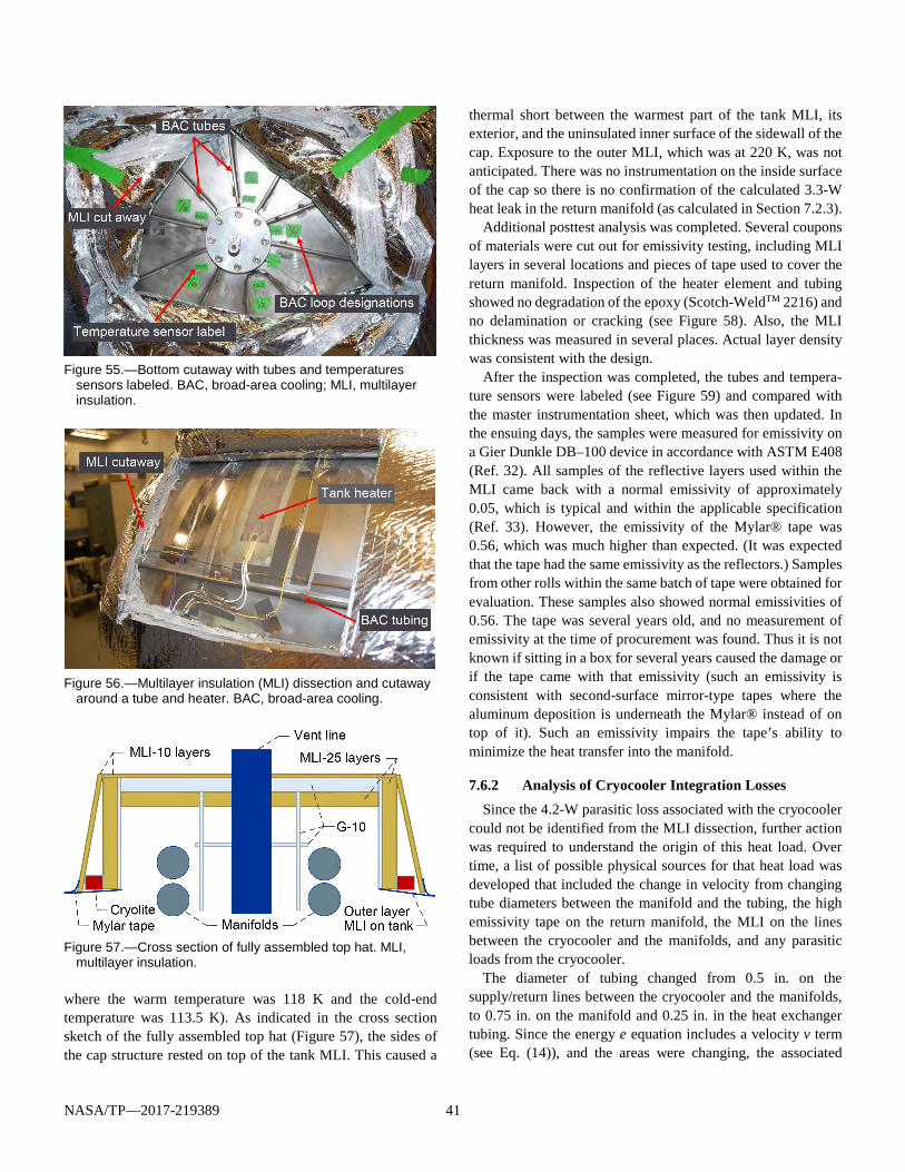
NASA/TP—2017-219389 41

Figure 55.—Bottom cutaway with tubes and temperatures

sensors labeled. BAC, broad-area cooling; MLI, multilayer insulation.

Figure 56.—Multilayer insulation (MLI) dissection and cutaway

around a tube and heater. BAC, broad-area cooling.

Figure 57.—Cross section of fully assembled top hat. MLI,

multilayer insulation.

where the warm temperature was 118 K and the cold-end temperature was 113.5 K). As indicated in the cross section sketch of the fully assembled top hat (Figure 57), the sides of the cap structure rested on top of the tank MLI. This caused a

thermal short between the warmest part of the tank MLI, its exterior, and the uninsulated inner surface of the sidewall of the cap. Exposure to the outer MLI, which was at 220 K, was not anticipated. There was no instrumentation on the inside surface of the cap so there is no confirmation of the calculated 3.3-W heat leak in the return manifold (as calculated in Section 7.2.3).

Additional posttest analysis was completed. Several coupons of materials were cut out for emissivity testing, including MLI layers in several locations and pieces of tape used to cover the return manifold. Inspection of the heater element and tubing showed no degradation of the epoxy (Scotch-WeldTM 2216) and no delamination or cracking (see Figure 58). Also, the MLI thickness was measured in several places. Actual layer density was consistent with the design.

After the inspection was completed, the tubes and tempera-ture sensors were labeled (see Figure 59) and compared with the master instrumentation sheet, which was then updated. In the ensuing days, the samples were measured for emissivity on a Gier Dunkle DB–100 device in accordance with ASTM E408 (Ref. 32). All samples of the reflective layers used within the MLI came back with a normal emissivity of approximately 0.05, which is typical and within the applicable specification (Ref. 33). However, the emissivity of the Mylar® tape was 0.56, which was much higher than expected. (It was expected that the tape had the same emissivity as the reflectors.) Samples from other rolls within the same batch of tape were obtained for evaluation. These samples also showed normal emissivities of 0.56. The tape was several years old, and no measurement of emissivity at the time of procurement was found. Thus it is not known if sitting in a box for several years caused the damage or if the tape came with that emissivity (such an emissivity is consistent with second-surface mirror-type tapes where the aluminum deposition is underneath the Mylar® instead of on top of it). Such an emissivity impairs the tape’s ability to minimize the heat transfer into the manifold.

7.6.2 Analysis of Cryocooler Integration Losses Since the 4.2-W parasitic loss associated with the cryocooler

could not be identified from the MLI dissection, further action was required to understand the origin of this heat load. Over time, a list of possible physical sources for that heat load was developed that included the change in velocity from changing tube diameters between the manifold and the tubing, the high emissivity tape on the return manifold, the MLI on the lines between the cryocooler and the manifolds, and any parasitic loads from the cryocooler.

The diameter of tubing changed from 0.5 in. on the supply/return lines between the cryocooler and the manifolds, to 0.75 in. on the manifold and 0.25 in. in the heat exchanger tubing. Since the energy e equation includes a velocity v term (see Eq. (14)), and the areas were changing, the associated

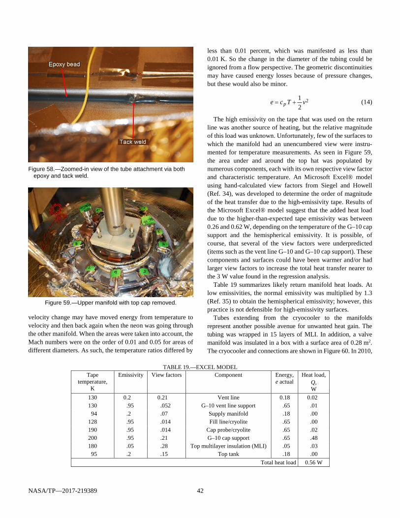
NASA/TP—2017-219389 42

Figure 58.—Zoomed-in view of the tube attachment via both

epoxy and tack weld.

Figure 59.—Upper manifold with top cap removed.

velocity change may have moved energy from temperature to velocity and then back again when the neon was going through the other manifold. When the areas were taken into account, the Mach numbers were on the order of 0.01 and 0.05 for areas of different diameters. As such, the temperature ratios differed by

less than 0.01 percent, which was manifested as less than 0.01 K. So the change in the diameter of the tubing could be ignored from a flow perspective. The geometric discontinuities may have caused energy losses because of pressure changes, but these would also be minor.

212pe c T v= + (14)

The high emissivity on the tape that was used on the return line was another source of heating, but the relative magnitude of this load was unknown. Unfortunately, few of the surfaces to which the manifold had an unencumbered view were instru-mented for temperature measurements. As seen in Figure 59, the area under and around the top hat was populated by numerous components, each with its own respective view factor and characteristic temperature. An Microsoft Excel® model using hand-calculated view factors from Siegel and Howell (Ref. 34), was developed to determine the order of magnitude of the heat transfer due to the high-emissivity tape. Results of the Microsoft Excel® model suggest that the added heat load due to the higher-than-expected tape emissivity was between 0.26 and 0.62 W, depending on the temperature of the G–10 cap support and the hemispherical emissivity. It is possible, of course, that several of the view factors were underpredicted (items such as the vent line G–10 and G–10 cap support). These components and surfaces could have been warmer and/or had larger view factors to increase the total heat transfer nearer to the 3 W value found in the regression analysis.

Table 19 summarizes likely return manifold heat loads. At low emissivities, the normal emissivity was multiplied by 1.3 (Ref. 35) to obtain the hemispherical emissivity; however, this practice is not defensible for high-emissivity surfaces.

Tubes extending from the cryocooler to the manifolds represent another possible avenue for unwanted heat gain. The tubing was wrapped in 15 layers of MLI. In addition, a valve manifold was insulated in a box with a surface area of 0.28 m2. The cryocooler and connections are shown in Figure 60. In 2010,

TABLE 19.—EXCEL MODEL

Tape temperature,

K

Emissivity View factors Component Energy, e actual

Heat load, Q, W

130 0.2 0.21 Vent line 0.18 0.02 130 .95 .052 G–10 vent line support .65 .01

94 .2 .07 Supply manifold .18 .00 128 .95 .014 Fill line/cryolite .65 .00 190 .95 .014 Cap probe/cryolite .65 .02 200 .95 .21 G–10 cap support .65 .48 180 .05 .28 Top multilayer insulation (MLI) .05 .03

95 .2 .15 Top tank .18 .00 Total heat load 0.56 W

NASA/TP—2017-219389 43

a team of researchers built and tested several MLI systems on small-diameter tubing at the NASA Kennedy Space Center, installing each layer individually (Ref. 36). Researchers found heat loads between 0.75 to 1 W/m (length of line) at warm boundary temperatures of 300 K. Reducing the warm boundary temperature to 220 K should give a heat transfer reduction of about a factor of 2. Thus, with well-insulated lines, the heat load is expected to be just below a 0.5 W/m⋅(length of line). However, instead of being installed individually, one layer at a time (as was done in the course of Kennedy testing), the MLI layers on the tubing were simultaneously wrapped in a spiral fashion. Because of the geometry and tube sizes, this meant that the seam along the 15 layers of MLI was approximately 2.7 times longer than the actual tubing. On the basis of the model

developed by Hinckley (Ref. 37) for this configuration, the seam heat load should be 0.14 W/m of seam, or 0.38 W/m of tubing, with a total heat load of at least 0.9 W/m of tubing. From these parameters, the total heat load through the MLI portion was estimated to be between 1.9 and 2.6 W, nominally 2.2 W.

There is also a thermal parasitic heat load associated with the RTBC refrigeration cycle (which is documented in Ref. 38) as

par TA,corr loss, recup liftQ Q Q Q= − − (15)

where recup indicates recuperative. This loss averaged 0.43 W over the test matrix.

Total losses calculated from these assessments were between 2.6 and 3.7 W. The remainder of the 4.2-W disparity cannot be explained with available data.

Figure 60.—Cryocooler broad-area cooling (BAC) supply and return lines and valve manifold.

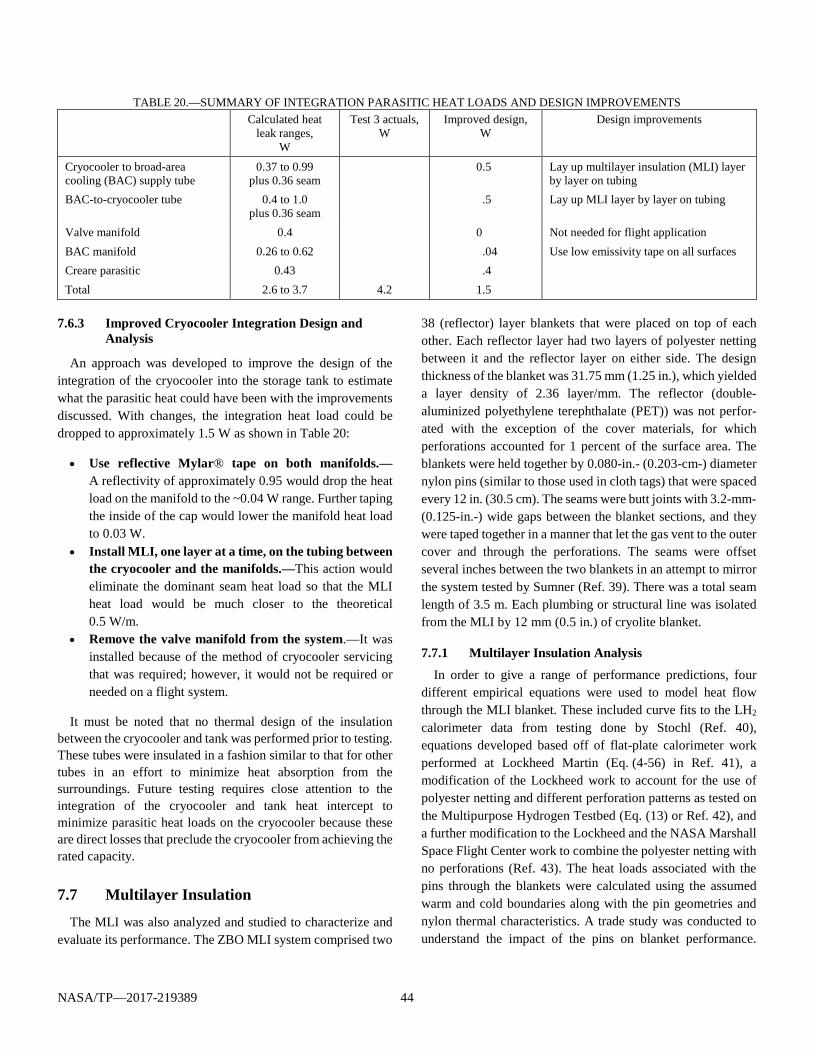
NASA/TP—2017-219389 44

TABLE 20.—SUMMARY OF INTEGRATION PARASITIC HEAT LOADS AND DESIGN IMPROVEMENTS Calculated heat

leak ranges, W

Test 3 actuals, W

Improved design, W

Design improvements

Cryocooler to broad-area cooling (BAC) supply tube

0.37 to 0.99 plus 0.36 seam

0.5 Lay up multilayer insulation (MLI) layer by layer on tubing

BAC-to-cryocooler tube 0.4 to 1.0 plus 0.36 seam

.5 Lay up MLI layer by layer on tubing

Valve manifold 0.4 0 Not needed for flight application BAC manifold 0.26 to 0.62 .04 Use low emissivity tape on all surfaces Creare parasitic 0.43 .4 Total 2.6 to 3.7 4.2 1.5

7.6.3 Improved Cryocooler Integration Design and Analysis

An approach was developed to improve the design of the integration of the cryocooler into the storage tank to estimate what the parasitic heat could have been with the improvements discussed. With changes, the integration heat load could be dropped to approximately 1.5 W as shown in Table 20:

• Use reflective Mylar® tape on both manifolds.—A reflectivity of approximately 0.95 would drop the heat load on the manifold to the ~0.04 W range. Further taping the inside of the cap would lower the manifold heat load to 0.03 W.

• Install MLI, one layer at a time, on the tubing between the cryocooler and the manifolds.—This action would eliminate the dominant seam heat load so that the MLI heat load would be much closer to the theoretical 0.5 W/m.

• Remove the valve manifold from the system.—It was installed because of the method of cryocooler servicing that was required; however, it would not be required or needed on a flight system.

It must be noted that no thermal design of the insulation between the cryocooler and tank was performed prior to testing. These tubes were insulated in a fashion similar to that for other tubes in an effort to minimize heat absorption from the surroundings. Future testing requires close attention to the integration of the cryocooler and tank heat intercept to minimize parasitic heat loads on the cryocooler because these are direct losses that preclude the cryocooler from achieving the rated capacity.

7.7 Multilayer Insulation

The MLI was also analyzed and studied to characterize and evaluate its performance. The ZBO MLI system comprised two

38 (reflector) layer blankets that were placed on top of each other. Each reflector layer had two layers of polyester netting between it and the reflector layer on either side. The design thickness of the blanket was 31.75 mm (1.25 in.), which yielded a layer density of 2.36 layer/mm. The reflector (double-aluminized polyethylene terephthalate (PET)) was not perfor-ated with the exception of the cover materials, for which perforations accounted for 1 percent of the surface area. The blankets were held together by 0.080-in.- (0.203-cm-) diameter nylon pins (similar to those used in cloth tags) that were spaced every 12 in. (30.5 cm). The seams were butt joints with 3.2-mm-(0.125-in.-) wide gaps between the blanket sections, and they were taped together in a manner that let the gas vent to the outer cover and through the perforations. The seams were offset several inches between the two blankets in an attempt to mirror the system tested by Sumner (Ref. 39). There was a total seam length of 3.5 m. Each plumbing or structural line was isolated from the MLI by 12 mm (0.5 in.) of cryolite blanket.

7.7.1 Multilayer Insulation Analysis In order to give a range of performance predictions, four

different empirical equations were used to model heat flow through the MLI blanket. These included curve fits to the LH2

calorimeter data from testing done by Stochl (Ref. 40), equations developed based off of flat-plate calorimeter work performed at Lockheed Martin (Eq. (4-56) in Ref. 41), a modification of the Lockheed work to account for the use of polyester netting and different perforation patterns as tested on the Multipurpose Hydrogen Testbed (Eq. (13) or Ref. 42), and a further modification to the Lockheed and the NASA Marshall Space Flight Center work to combine the polyester netting with no perforations (Ref. 43). The heat loads associated with the pins through the blankets were calculated using the assumed warm and cold boundaries along with the pin geometries and nylon thermal characteristics. A trade study was conducted to understand the impact of the pins on blanket performance.

NASA/TP—2017-219389 45

Results of the trade study are shown in Figure 61 and Table 21 and led to the design spacing of 0.31 m (12 in.). The Stochl (Ref. 40) calorimeter equations were used in the trade study.

To model the seams, data from a Sumner paper were used initially (Ref. 39); however, that study had a different seam width, number of layers, and seam offset spacing. The analysis was simplified with an assumption that the two seams were one and by using equations from Hinckley (Ref. 37) to predict the heat loads. The cryolite thermal isolation penalties for the vent line, fill line, capacitance probe, and six struts were calculated using the equations derived by Johnson and Kelly (Ref. 24). Table 22 shows the individual heat loads on the different components.

In comparing the predicted performance versus the total performance, two measures were used. The first was the MLI-blanket-based scale factor—the ratio between the actual test heat load and the MLI heat load:

actualblanket

MLI

QSFQ

= (16)

The other metric was the system scale factor—the ratio of the actual heat load to the total heat load predicted through the MLI. The actual test heat load was 2.6 W with the warm boundary

temperature at 220 K and was 4.8 W with the warm boundary temperature at 300 K. Test results are shown in Table 23 and Table 24.

actualsys

MLI pin seam pen

QSFQ Q Q Q

=+ + +

(17)

Figure 61.—Effect of pin conductance on zero boiloff

(ZBO) multilayer insulation (MLI) blanket performance.

TABLE 21.—EFFECT OF PIN CONDUCTANCE ON ZERO BOILOFF (ZBO) MULTILAYER

INSULATION (MLI) BLANKET PERFORMANCE [ZBO tank conventional blanket heat leak breakup; warm and cold boundary temperatures,

250 and 90 K, respectively; 75 layers, 0.080 in. diameter, 1.1-in.-long nylon pin.] Pin distance,

in. Blanket,

W/m2 Pins/m2, no./m2

Pins, W/m2

Total, W/m2

Heat leak of pins,

percent 4 0.146 97 0.668 0.814 82.1 8 24 .167 .313 53.4

12 11 .074 .220 33.7 16 6 .042 .188 22.2 20 4 .027 .173 15.5 24 3 .019 .165 11.3

TABLE 22.—MULTILAYER INSULATION (MLI)

COMPONENT HEAT LOADS Component Heat load, W

Warm boundary temperature, K 220 300

Pins 0.298 0.53 Seams .390 1.32 Penetrations .250 .40 Total .938 2.25

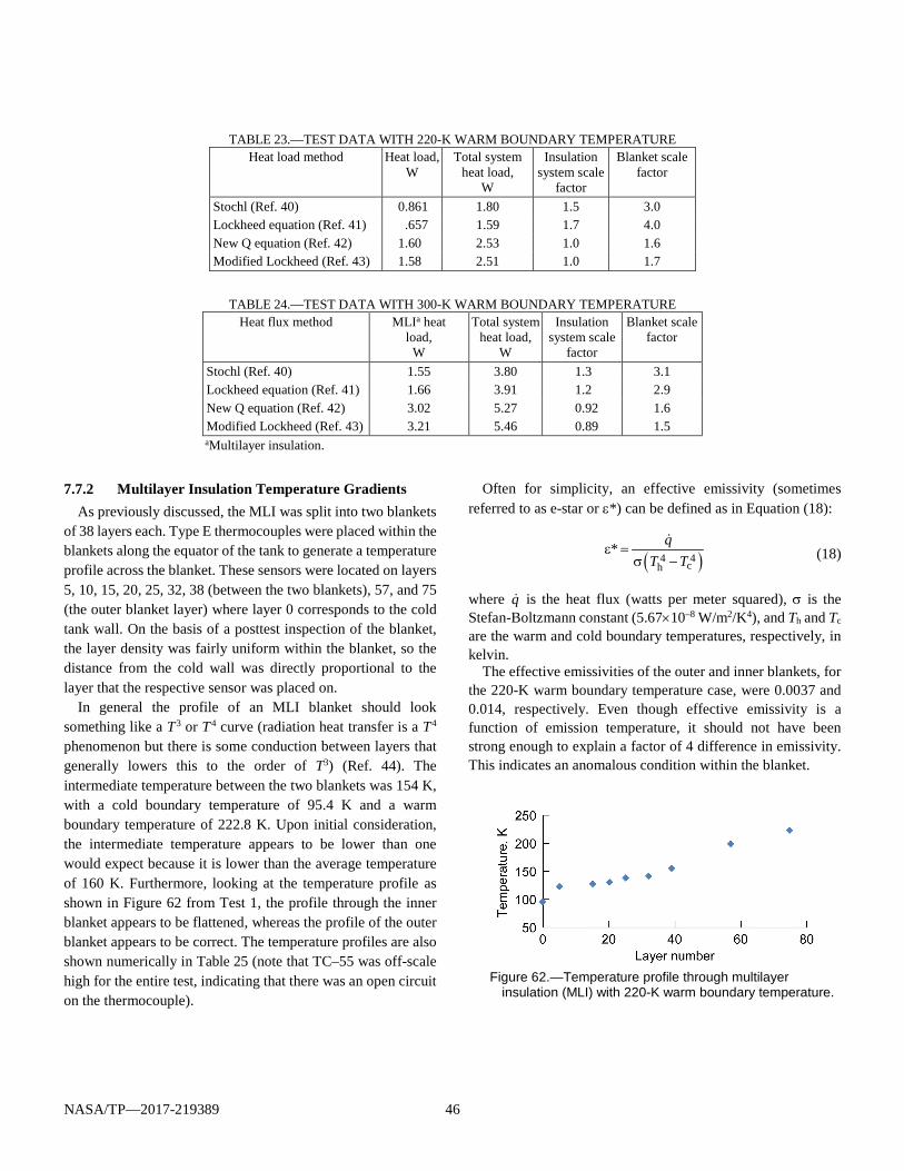
NASA/TP—2017-219389 46

TABLE 23.—TEST DATA WITH 220-K WARM BOUNDARY TEMPERATURE

Heat load method Heat load, W

Total system heat load,

W

Insulation system scale

factor

Blanket scale factor

Stochl (Ref. 40) 0.861 1.80 1.5 3.0 Lockheed equation (Ref. 41) .657 1.59 1.7 4.0 New Q equation (Ref. 42) 1.60 2.53 1.0 1.6 Modified Lockheed (Ref. 43) 1.58 2.51 1.0 1.7

TABLE 24.—TEST DATA WITH 300-K WARM BOUNDARY TEMPERATURE

Heat flux method MLIa heat load,

W

Total system heat load,

W

Insulation system scale

factor

Blanket scale factor

Stochl (Ref. 40) 1.55 3.80 1.3 3.1 Lockheed equation (Ref. 41) 1.66 3.91 1.2 2.9 New Q equation (Ref. 42) 3.02 5.27 0.92 1.6 Modified Lockheed (Ref. 43) 3.21 5.46 0.89 1.5 aMultilayer insulation.

7.7.2 Multilayer Insulation Temperature Gradients As previously discussed, the MLI was split into two blankets

of 38 layers each. Type E thermocouples were placed within the blankets along the equator of the tank to generate a temperature profile across the blanket. These sensors were located on layers 5, 10, 15, 20, 25, 32, 38 (between the two blankets), 57, and 75 (the outer blanket layer) where layer 0 corresponds to the cold tank wall. On the basis of a posttest inspection of the blanket, the layer density was fairly uniform within the blanket, so the distance from the cold wall was directly proportional to the layer that the respective sensor was placed on.

In general the profile of an MLI blanket should look something like a T

3 or T 4 curve (radiation heat transfer is a T

4 phenomenon but there is some conduction between layers that generally lowers this to the order of T3) (Ref. 44). The intermediate temperature between the two blankets was 154 K, with a cold boundary temperature of 95.4 K and a warm boundary temperature of 222.8 K. Upon initial consideration, the intermediate temperature appears to be lower than one would expect because it is lower than the average temperature of 160 K. Furthermore, looking at the temperature profile as shown in Figure 62 from Test 1, the profile through the inner blanket appears to be flattened, whereas the profile of the outer blanket appears to be correct. The temperature profiles are also shown numerically in Table 25 (note that TC–55 was off-scale high for the entire test, indicating that there was an open circuit on the thermocouple).

Often for simplicity, an effective emissivity (sometimes referred to as e-star or ε*) can be defined as in Equation (18):

( )4 4

ch* q

T Tε =

σ −

(18)

where q is the heat flux (watts per meter squared), σ is the Stefan-Boltzmann constant (5.67×10–8 W/m2/K4), and Th and Tc are the warm and cold boundary temperatures, respectively, in kelvin.

The effective emissivities of the outer and inner blankets, for the 220-K warm boundary temperature case, were 0.0037 and 0.014, respectively. Even though effective emissivity is a function of emission temperature, it should not have been strong enough to explain a factor of 4 difference in emissivity. This indicates an anomalous condition within the blanket.

Figure 62.—Temperature profile through multilayer

insulation (MLI) with 220-K warm boundary temperature.

NASA/TP—2017-219389 47

Figure 63.—Temperature profile through multilayer

insulation (MLI) with 300-K warm boundary temperature. For a similar analysis of Test 10 at a warm boundary tempera-

ture of 300 K, the profile looks much different (Figure 63). The curve form better resembles a third-order function, and the intermediate temperature between the two blankets was 227 K, which is greater than the mean blanket temperature of 191 K. Comparing blanket effective emissivities again, the inner blanket had an effective emissivity of 0.0050 and the outer blanket had an effective emissivity of 0.0023. Although this is still a factor of 2 different, it is much closer than that observed for the 220-K test.

It should be noted that nothing was done to the blanket between tests; the article was not removed from the vacuum chamber, nor were any vacuum pumping cycles attempted. This rules out the possibility that the blanket was affected by a physical change. Also, the temperature profiles of all tests run at 220-K warm boundary temperature were essentially identical. This was not a gradual change over time that could be attributed to further evacuation of the blanket.

A logical conclusion is that there are temperature-based func-tional performance issues occurring at low temperatures, even up to the 150-K regime. Previous investigators noticed emis-sivity issues at temperatures between 20 and 90 K (Refs. 45 and 46). However, the present result would stretch the warm temperature effects higher than that.

7.8 Radiator Performance The radiator (see Figure 12) performed nominally, with an

average interface temperature of 260 K and an average gradient on each of the two panels of 4.1 and 1.3 K while the cryocooler and tank heat were being removed for each of the active thermal control tests. The radiator’s outer surface was painted white with AZ–93 paint and had an emissivity of 0.95 and a measured efficiency of 98.4 percent. The inner surface was insulated with a 10-layer MLI blanket. The radiator design specified a thermal gradient of less than 6 K while rejecting 400 W, or 200 W per panel, at 300 K. The ZBO radiator test data is shown in

Figure 64.—Radiator panel A and B bench test data

plotted with zero boiloff (ZBO) test data.

TABLE 25.—TEMPERATURE PROFILE THROUGH MULTILAYER INSULATION (MLI) FOR WARM

BOUNDARY TEMPERATURES OF 220 AND 300 K Sensora Layer

(from bottom) Warm boundary temperature, K

220 300 Shroud --- 218.8 298.4 TC–51 75 222.8 302.8 TC–52 57 199.1 274.0 TC–53 39 154.2 226.9 TC–59 32 140.8 206.3 TC–58 25 137.3 197.6 TC–57 20 131.1 183.0 TC–56 15 127.4 174.0 TC–55 10 Off-scale high Off-scale high TC–54 5 121.6 132.8

(b) 0 95.4 78.6 aTC, thermocouple. bCold boundary temperature.

Figure 64, along with the bench test data on each radiator panel. The measured radiator panel heat flow at the panel temperature was consistent with that found in radiator panel bench testing at the vendor, where the radiator rejected up to 200 W while maintaining a radiator interface plate temperature of 296 K or higher. With each panel’s surface area being 0.84 m2, the panel heat flux was 238 W/m2.

8.0 Discussion of Results 8.1 Component Performance

This section is included to compare the performance of principle system components (see Table 26) with pretest

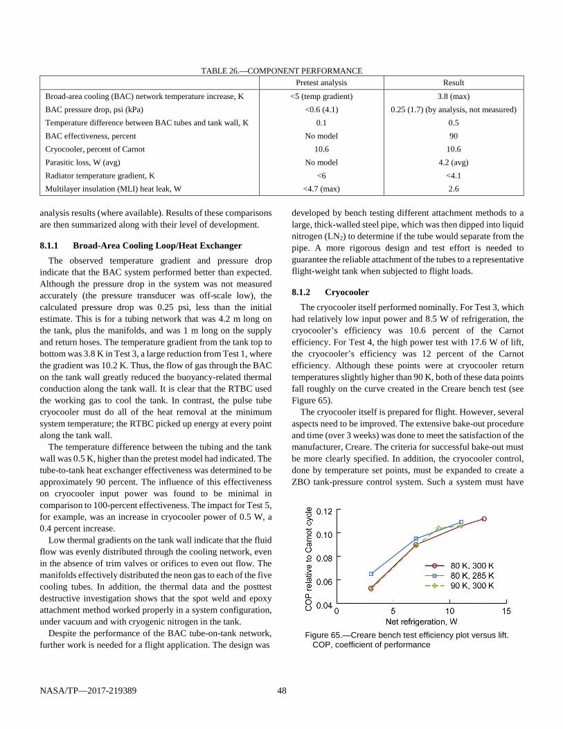
NASA/TP—2017-219389 48

TABLE 26.—COMPONENT PERFORMANCE Pretest analysis Result

Broad-area cooling (BAC) network temperature increase, K <5 (temp gradient) 3.8 (max) BAC pressure drop, psi (kPa) <0.6 (4.1) 0.25 (1.7) (by analysis, not measured) Temperature difference between BAC tubes and tank wall, K 0.1 0.5 BAC effectiveness, percent No model 90 Cryocooler, percent of Carnot 10.6 10.6 Parasitic loss, W (avg) No model 4.2 (avg) Radiator temperature gradient, K <6 <4.1 Multilayer insulation (MLI) heat leak, W <4.7 (max) 2.6

analysis results (where available). Results of these comparisons are then summarized along with their level of development.

8.1.1 Broad-Area Cooling Loop/Heat Exchanger The observed temperature gradient and pressure drop

indicate that the BAC system performed better than expected. Although the pressure drop in the system was not measured accurately (the pressure transducer was off-scale low), the calculated pressure drop was 0.25 psi, less than the initial estimate. This is for a tubing network that was 4.2 m long on the tank, plus the manifolds, and was 1 m long on the supply and return hoses. The temperature gradient from the tank top to bottom was 3.8 K in Test 3, a large reduction from Test 1, where the gradient was 10.2 K. Thus, the flow of gas through the BAC on the tank wall greatly reduced the buoyancy-related thermal conduction along the tank wall. It is clear that the RTBC used the working gas to cool the tank. In contrast, the pulse tube cryocooler must do all of the heat removal at the minimum system temperature; the RTBC picked up energy at every point along the tank wall.

The temperature difference between the tubing and the tank wall was 0.5 K, higher than the pretest model had indicated. The tube-to-tank heat exchanger effectiveness was determined to be approximately 90 percent. The influence of this effectiveness on cryocooler input power was found to be minimal in comparison to 100-percent effectiveness. The impact for Test 5, for example, was an increase in cryocooler power of 0.5 W, a 0.4 percent increase.

Low thermal gradients on the tank wall indicate that the fluid flow was evenly distributed through the cooling network, even in the absence of trim valves or orifices to even out flow. The manifolds effectively distributed the neon gas to each of the five cooling tubes. In addition, the thermal data and the posttest destructive investigation shows that the spot weld and epoxy attachment method worked properly in a system configuration, under vacuum and with cryogenic nitrogen in the tank.

Despite the performance of the BAC tube-on-tank network, further work is needed for a flight application. The design was

developed by bench testing different attachment methods to a large, thick-walled steel pipe, which was then dipped into liquid nitrogen (LN2) to determine if the tube would separate from the pipe. A more rigorous design and test effort is needed to guarantee the reliable attachment of the tubes to a representative flight-weight tank when subjected to flight loads.

8.1.2 Cryocooler The cryocooler itself performed nominally. For Test 3, which

had relatively low input power and 8.5 W of refrigeration, the cryocooler’s efficiency was 10.6 percent of the Carnot efficiency. For Test 4, the high power test with 17.6 W of lift, the cryocooler’s efficiency was 12 percent of the Carnot efficiency. Although these points were at cryocooler return temperatures slightly higher than 90 K, both of these data points fall roughly on the curve created in the Creare bench test (see Figure 65).

The cryocooler itself is prepared for flight. However, several aspects need to be improved. The extensive bake-out procedure and time (over 3 weeks) was done to meet the satisfaction of the manufacturer, Creare. The criteria for successful bake-out must be more clearly specified. In addition, the cryocooler control, done by temperature set points, must be expanded to create a ZBO tank-pressure control system. Such a system must have

Figure 65.—Creare bench test efficiency plot versus lift.

COP, coefficient of performance

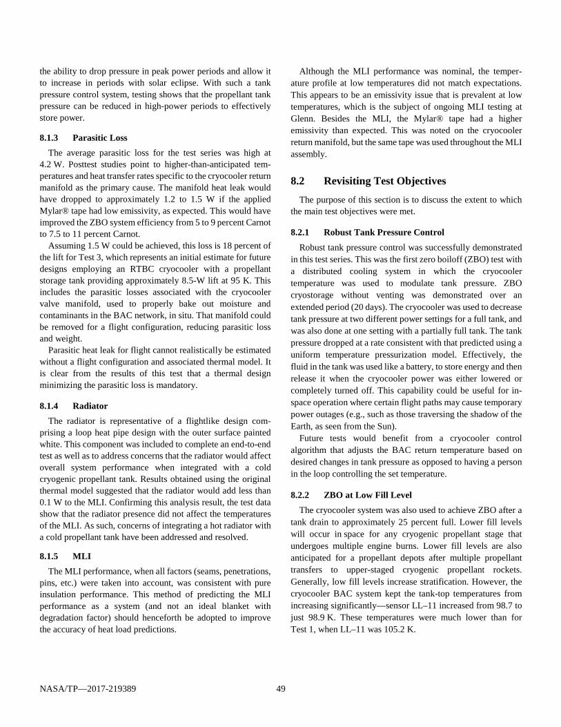
NASA/TP—2017-219389 49

the ability to drop pressure in peak power periods and allow it to increase in periods with solar eclipse. With such a tank pressure control system, testing shows that the propellant tank pressure can be reduced in high-power periods to effectively store power.

8.1.3 Parasitic Loss The average parasitic loss for the test series was high at

4.2 W. Posttest studies point to higher-than-anticipated tem-peratures and heat transfer rates specific to the cryocooler return manifold as the primary cause. The manifold heat leak would have dropped to approximately 1.2 to 1.5 W if the applied Mylar® tape had low emissivity, as expected. This would have improved the ZBO system efficiency from 5 to 9 percent Carnot to 7.5 to 11 percent Carnot.

Assuming 1.5 W could be achieved, this loss is 18 percent of the lift for Test 3, which represents an initial estimate for future designs employing an RTBC cryocooler with a propellant storage tank providing approximately 8.5-W lift at 95 K. This includes the parasitic losses associated with the cryocooler valve manifold, used to properly bake out moisture and contaminants in the BAC network, in situ. That manifold could be removed for a flight configuration, reducing parasitic loss and weight.

Parasitic heat leak for flight cannot realistically be estimated without a flight configuration and associated thermal model. It is clear from the results of this test that a thermal design minimizing the parasitic loss is mandatory.

8.1.4 Radiator The radiator is representative of a flightlike design com-

prising a loop heat pipe design with the outer surface painted white. This component was included to complete an end-to-end test as well as to address concerns that the radiator would affect overall system performance when integrated with a cold cryogenic propellant tank. Results obtained using the original thermal model suggested that the radiator would add less than 0.1 W to the MLI. Confirming this analysis result, the test data show that the radiator presence did not affect the temperatures of the MLI. As such, concerns of integrating a hot radiator with a cold propellant tank have been addressed and resolved.

8.1.5 MLI The MLI performance, when all factors (seams, penetrations,

pins, etc.) were taken into account, was consistent with pure insulation performance. This method of predicting the MLI performance as a system (and not an ideal blanket with degradation factor) should henceforth be adopted to improve the accuracy of heat load predictions.

Although the MLI performance was nominal, the temper-ature profile at low temperatures did not match expectations. This appears to be an emissivity issue that is prevalent at low temperatures, which is the subject of ongoing MLI testing at Glenn. Besides the MLI, the Mylar® tape had a higher emissivity than expected. This was noted on the cryocooler return manifold, but the same tape was used throughout the MLI assembly.

8.2 Revisiting Test Objectives The purpose of this section is to discuss the extent to which

the main test objectives were met.

8.2.1 Robust Tank Pressure Control Robust tank pressure control was successfully demonstrated

in this test series. This was the first zero boiloff (ZBO) test with a distributed cooling system in which the cryocooler temperature was used to modulate tank pressure. ZBO cryostorage without venting was demonstrated over an extended period (20 days). The cryocooler was used to decrease tank pressure at two different power settings for a full tank, and was also done at one setting with a partially full tank. The tank pressure dropped at a rate consistent with that predicted using a uniform temperature pressurization model. Effectively, the fluid in the tank was used like a battery, to store energy and then release it when the cryocooler power was either lowered or completely turned off. This capability could be useful for in-space operation where certain flight paths may cause temporary power outages (e.g., such as those traversing the shadow of the Earth, as seen from the Sun).

Future tests would benefit from a cryocooler control algorithm that adjusts the BAC return temperature based on desired changes in tank pressure as opposed to having a person in the loop controlling the set temperature.

8.2.2 ZBO at Low Fill Level The cryocooler system was also used to achieve ZBO after a

tank drain to approximately 25 percent full. Lower fill levels will occur in space for any cryogenic propellant stage that undergoes multiple engine burns. Lower fill levels are also anticipated for a propellant depots after multiple propellant transfers to upper-staged cryogenic propellant rockets. Generally, low fill levels increase stratification. However, the cryocooler BAC system kept the tank-top temperatures from increasing significantly—sensor LL–11 increased from 98.7 to just 98.9 K. These temperatures were much lower than for Test 1, when LL–11 was 105.2 K.

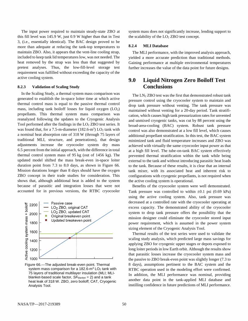
NASA/TP—2017-219389 50

The input power required to maintain steady-state ZBO at this fill level was 145.9 W, just 0.9 W higher than that in Test 3, (i.e., essentially identical). The BAC design proved to be more than adequate at reducing the tank-top temperatures to maintain ZBO. Also, it appears that the vent-line cooling strap, included to keep tank lid temperatures low, was not needed. The heat removed by the strap was less than that suggested by pretest analyses. Thus, the low-fill-level storage test requirement was fulfilled without exceeding the capacity of the active cooling system.

8.2.3 Validation of Scaling Study In the Scaling Study, a thermal system mass comparison was

generated to establish the in-space loiter time at which active thermal control mass is equal to the passive thermal control mass, including tank boiloff losses for liquid oxygen (LO2) propellants. This thermal system mass comparison was reanalyzed following the updates to the Cryogenic Analysis Tool performed after the findings in the LO2 ZBO test series. It was found that, for a 7.5-m-diameter (182.6-m3) LO2 tank with a nominal heat absorption rate of 318 W (through 75 layers of traditional MLI, structure, and penetrations), that design adjustments increase the cryocooler system dry mass 6.5 percent from the initial approach, with the difference in total thermal control system mass of 95 kg (out of 1456 kg). The updated model shifted the mass break-even in-space loiter duration point from 7.3 to 8.0 days, as shown in Figure 66. Mission durations longer than 8 days should have the oxygen ZBO concept in their trade studies for consideration. This shows that, although additional heat is added to the system because of parasitic and integration losses that were not accounted for in previous versions, the RTBC cryocooler

Figure 66.—The adjusted break-even point. Thermal

system mass comparison for a 182.6-m3 LO2 tank with 75 layers of traditional multilayer insulation (MLI; MLI-blanket-based scale factor, SFblanket = 2) and a tank heat leak of 318 W. ZBO, zero boiloff; CAT, Cryogenic Analysis Tool.

system mass does not significantly increase, lending support to the scalability of the LO2 ZBO test concept.

8.2.4 MLI Database The MLI performance, with the improved analysis approach,

yielded a more accurate prediction than traditional methods. Gaining performance at multiple environmental temperatures further increases the value of the data point for future designs.

9.0 Liquid Nitrogen Zero Boiloff Test Conclusions

The LN2 ZBO test was the first that demonstrated robust tank pressure control using the cryocooler system to maintain and drop tank pressure without venting. The tank pressure was maintained without venting for a 20-day period. Tank stratifi-cation, which causes high tank pressurization rates for unvented and unmixed cryogenic tanks, was cut by 88 percent using the broad-area-cooling (BAC) system. Robust tank pressure control was also demonstrated at a low fill level, which causes additional propellant stratification. In this test, the BAC system minimized tank and fluid temperature increases and ZBO was achieved with virtually the same cryocooler input power as that at a high fill level. The tube-on-tank BAC system effectively prevented thermal stratification within the tank while being external to the tank and without introducing parasitic heat loads to the tank. Because of these results, it is clear that an internal tank mixer, with its associated heat and inherent risk to configurations with cryogenic propellants, is not required when the active cooling system is operational.

Benefits of the cryocooler system were well demonstrated. Tank pressure was controlled to within ±0.1 psi (0.69 kPa) using the active cooling system. Also, tank pressure was decreased at a controlled rate with the cryocooler operating at excess capacity. The demonstrated ability of the cryocooler system to drop tank pressure offers the possibility that the mission designer could eliminate the cryocooler stored input power requirement, which is assumed in the power system sizing element of the Cryogenic Analysis Tool.

Thermal results of the test series were used to validate the scaling study analysis, which predicted large mass savings for applying ZBO for cryogenic upper stages or depots exposed to long loiter periods in low Earth orbit. Although the results show that parasitic losses increase the cryocooler system mass and the passive to ZBO break-even point was slightly longer (7.3 to 8 days), assumptions pertinent to the BAC system and the RTBC operation used in the modeling effort were confirmed. In addition, the MLI performance was nominal, providing another data point in the tank-applied MLI database and instilling confidence in future predictions of MLI performance.

NASA/TP—2017-219389 51

For a potential flight application, this test series has advanced the technology, reducing the risk for future flight projects. The integrated performance of the four main components—the cryocooler, the broad area cooling network, the multilayer insulation system, and the radiator—coupled to a cryogenic tank has increased confidence in this concept for flight. Work

remains, particularly on optimizing the tube-on-tank design, on cryocooler parasitic designs and implementation, and on low-temperature MLI behavior.

Glenn Research Center National Aeronautics and Space Administration Cleveland, Ohio, February 3, 2017

NASA/TP—2017-219389 53

Appendix A.—Symbols c specific heat COP coefficient of performance cp specific heat of the neon gas stream e energy h specific enthalpy

Kλ effective substrate-to-gas conductance L total tube length M mass m mass flow rate

P pressure Pcomp compressor power PTA recoverable turboalternator power R measured temperature rise rate per time, dT/dt Q heat load Qlift cooling capacity Quseful useful refrigeration

BOQ boiloff flow rate of the nitrogen

q heat flux

SFblanket MLI-blanket-based scale factor SFsys system scale factor T temperature t time T1 to T7 temperatures at Positions 1 to 7 Tc cold boundary temperature Th warm boundary temperature V volume v velocity

V volumetric flow rate of boiloff gas

x distance from the supply

ε fraction of Carnot

ε* effective emissivity

ηBAC heat transfer effectiveness of broad-area-cooling shield

ρ average density function

Subscripts BAC broad-area cooling or broad-area cooled BO boiloff bot mass of bottom part of tank byp voltage at bypass cc cryocooler cond conductance error measurement error f final state fill fill line gas gas flowing in the line heater tank wall heater instr instrumentation j volume segment linearized linearized value liq liquid loss, recup recuperative loss man, ret return manifold man, sup supply manifold MLI multilayer insulation nipple instrumentation nipple par parasitic on cooling loop pen penetration probe capacitance probe rake diode rake rej heat rejection ret return sup supply sys active cooling system t time tank tank; tank wall; total on tank top mass of top part of tank (part that is warmer

than rest of tank) tube tube wall vap vapor vent vent line wall tank wall wires wires 0 initial state

App

endi

x B

.—In

stru

men

tatio

n Ta

ble

27 to

Tab

le 2

9 sh

ow th

e si

licon

dio

des,

ther

moc

oupl

es, a

nd fa

cilit

y sy

stem

s ins

trum

enta

tion

used

in th

e ZB

O te

sts.

TA

BLE

27.—

SILI

CO

N D

IOD

E IN

STR

UM

ENTA

TIO

N

[SM

iRF,

Sm

all M

ulti-

Purp

ose

Res

earc

h Fa

cilit

y.]

LabV

IEW

TM

chan

nel

Des

crip

tion

SMiR

F lid

dio

de

plug

boar

d/si

gnal

& p

ower

SM

iRF

lid

feed

thro

ugh

Man

ufac

ture

r M

odel

nu

mbe

r Se

rial

num

ber

Cur

rent

so

urce

D

ata

acqu

isiti

on

chan

nel

LL–1

D

iode

rake

top—

at 9

5.6

perc

ent

1/1

& 2

5 FD

I1

Lake

shor

e D

T–67

0–SD

D

6032

284

PS 0

5 0

LL–2

D

iode

rake

—at

85.

1 pe

rcen

t 1/

2 FD

I1

Lake

shor

e D

T–67

0–SD

D

6032

388

PS 0

6 1

LL–3

D

iode

rake

—at

73.

7 pe

rcen

t 1/

3

FDI1

La

kesh

ore

DT–

670–

SD

D60

3228

8 PS

07

2 LL

–4

Dio

de ra

ke—

at 6

2 pe

rcen

t 1/

4 FD

I1

Lake

shor

e D

T–67

0–SD

D

6032

291

PS 0

8 3

LL–5

D

iode

rake

—at

38.

6 pe

rcen

t 1/

5 &

29

FDI1

La

kesh

ore

DT–

670–

SD

D60

3229

2 PS

09

4

LL–6

D

iode

rake

—at

26.

9 pe

rcen

t 1/

6 FD

I1

Lake

shor

e D

T–67

0–SD

D

6032

405

PS 1

0 5

LL–7

D

iode

rake

—at

15.

3 pe

rcen

t 1/

7

FDI1

La

kesh

ore

DT–

670–

SD

D60

3254

6 PS

11

6 LL

–8

Dio

de ra

ke b

otto

m—

at 0

.8 p

erce

nt

1/8

FDI2

La

kesh

ore

DT–

670–

SD

D60

3269

0 PS

12

7 LL

–9

Tube

10

mid

dle

tem

pera

ture

1/

9 &

33

FDI2

La

kesh

ore

DT–

670–

SD

D60

3233

4 PS

13

8 LL

–10

Tube

3 re

turn

tem

pera

ture

1/

10 &

34

FDI2

La

kesh

ore

DT–

670–

SD

D60

3171

4 PS

14

9

LL–1

1 Ta

nk to

p ne

ar 2

-in. v

ent

1/11

& 3

5 FD

I2

Lake

shor

e D

T–67

0–SD

D

6032

554

PS 1

5 10

LL

–12

Tank

bot

tom

nea

r tan

k sw

ay p

in

1/12

& 3

6 FD

I2

Lake

shor

e D

T–67

0–SD

D

6032

499

PS 1

6 11

LL

–13

Stru

t int

erfa

ce d

iode

(cen

ter b

otto

m e

dge)

1/

13 &

37

FDI2

La

kesh

ore

DT–

670–

SD

D60

3163

4 PS

17

12

LL–1

4 St

rut i

nter

face

dio

de (c

ente

r sid

e ed

ge)

1/14

& 3

8 FD

I2

Lake

shor

e D

T–67

0–SD

D

6031

648

PS 1

8 13

LL

–15

2-in

. ven

t int

erfa

ce o

n ta

nk

1/15

& 3

9 FD

I3

Lake

shor

e D

T–67

0–SD

D

6032

551

PS 1

9 14

LL–1

6 2-

in. v

ent i

nter

face

on

tank

1/

16 &

40

FDI3

La

kesh

ore

DT–

670–

SD

D60

3254

8 PS

20

15

LL–1

7 1-

in. f

ill in

terfa

ce o

n ta

nk

1/17

& 4

1 FD

I3

Lake

shor

e D

T–67

0–SD

D

6032

553

PS 2

1 16

LL

–18

1-in

. fill

inte

rface

on

tank

1/

18 &

42

FDI3

La

kesh

ore

DT–

670–

SD

D60

3273

6 PS

22

17

LL–1

9 In

stru

men

tatio

n po

rt in

terfa

ce o

n ta

nk

1/19

& 4

3 FD

I3

Lake

shor

e D

T–67

0–SD

D

6032

716

PS 2

3 18

LL

–20

Inst

rum

enta

tion

port

inte

rface

on

tank

1/

20 &

44

FDI3

La

kesh

ore

DT–

670–

SD

D60

3254

3 PS

24

19

SD

–1

Tank

wal

l bet

wee

n co

olin

g tu

bes 1

and

2

1/21

& 4

5 FD

I3

Lake

shor

e D

T–67

0–SD

D

6027

145

PS 2

5 20

SD

–2

Tank

wal

l bet

wee

n co

olin

g tu

bes 2

and

3

2/1

& 2

5 FD

I4

Lake

shor

e D

T–67

0–SD

D

6032

295

PS 2

6 21

SD

–3

Tank

wal

l bet

wee

n co

olin

g tu

bes 3

and

4

2/2

& 2

6 FD

I4

Lake

shor

e D

T–67

0–SD

D

6031

649

PS 2

7 22

SD

–4

Tank

wal

l bet

wee

n co

olin

g tu

bes 4

and

5

2/3

& 2

7 FD

I4

Lake

shor

e D

T–67

0–SD

D

6031

641

PS 2

8 23

SD

–5

Tank

wal

l bet

wee

n co

olin

g tu

bes 5

and

6

2/4

& 2

8 FD

I4

Lake

shor

e D

T–67

0–SD

D

6031

642

PS 2

9 24

SD

–6

Tank

wal

l bet

wee

n co

olin

g tu

bes 6

and

7

2/5

& 2

9 FD

I4

Lake

shor

e D

T–67

0–SD

D

6032

103

PS 3

0 25

SD

–7

Tank

wal

l bet

wee

n co

olin

g tu

bes 7

and

8

2/6

& 3

0 FD

I4

Lake

shor

e D

T–67

0–SD

D

6032

102

PS 3

1 26

SD

–8

Tank

wal

l bet

wee

n co

olin

g tu

bes 8

and

9

2/7

& 3

1 FD

I4

Lake

shor

e D

T–67

0–SD

D

6032

822

PS 3

2 27

SD

–9

Tank

wal

l bet

wee

n co

olin

g tu

bes 9

and

10

2/8

& 3

2 FD

I5

Lake

shor

e D

T–67

0–SD

D

6032

842

PS 3

3 28

SD

–10

Tank

wal

l bet

wee

n co

olin

g tu

bes 1

0 an

d 1

2/9

& 3

3 FD

I5

Lake

shor

e D

T–67

0–SD

D

6031

676

PS 3

4 29

NASA/TP—2017-219389 55

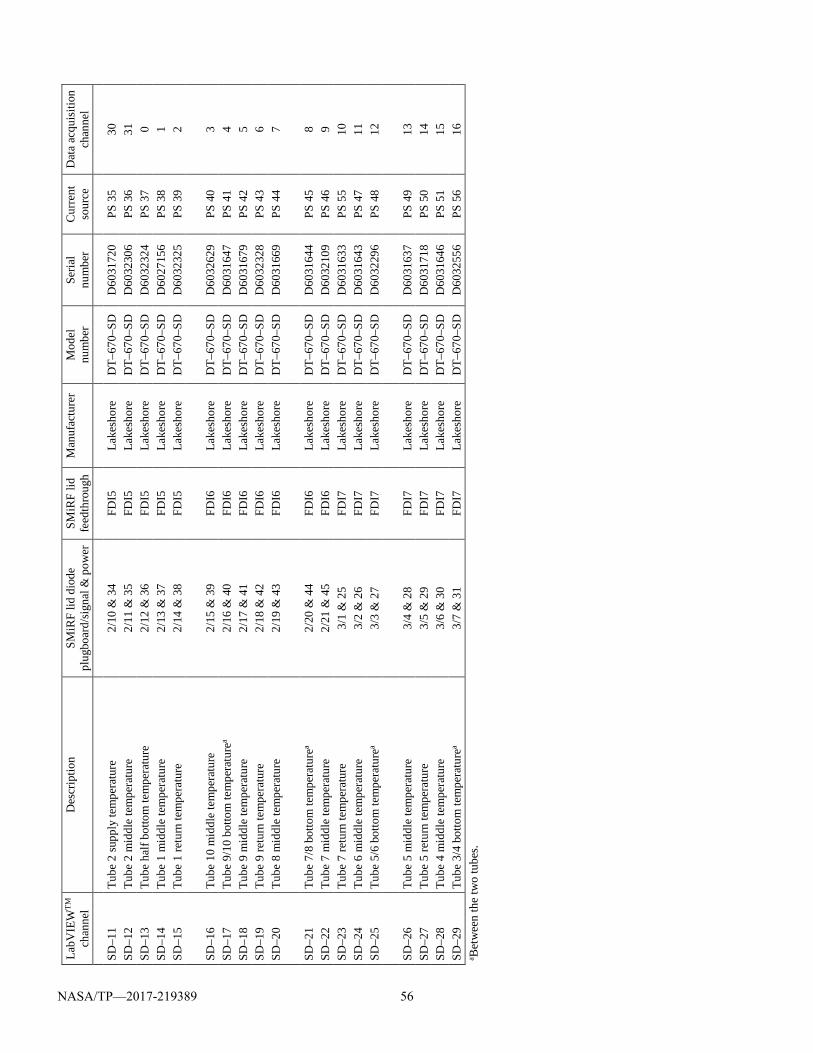
La

bVIE

WTM

ch

anne

l D

escr

iptio

n SM

iRF

lid d

iode

pl

ugbo

ard/

sign

al &

pow

er

SMiR

F lid

fe

edth

roug

h M

anuf

actu

rer

Mod

el

num

ber

Seria

l nu

mbe

r C

urre

nt

sour

ce

Dat

a ac

quis

ition

ch

anne

l

SD–1

1 Tu

be 2

supp

ly te

mpe

ratu

re

2/10

& 3

4 FD

I5

Lake

shor

e D

T–67

0–SD

D

6031

720

PS 3

5 30

SD

–12

Tube

2 m

iddl

e te

mpe

ratu

re

2/11

& 3

5 FD

I5

Lake

shor

e D

T–67

0–SD

D

6032

306

PS 3

6 31

SD

–13

Tube

hal

f bot

tom

tem

pera

ture

2/

12 &

36

FDI5

La

kesh

ore

DT–

670–

SD

D60

3232

4 PS

37

0 SD

–14

Tube

1 m

iddl

e te

mpe

ratu

re

2/13

& 3

7 FD

I5

Lake

shor

e D

T–67

0–SD

D

6027

156

PS 3

8 1

SD–1

5 Tu

be 1

retu

rn te

mpe

ratu

re

2/14

& 3

8 FD

I5

Lake

shor

e D

T–67

0–SD

D

6032

325

PS 3

9 2

SD

–16

Tube

10

mid

dle

tem

pera

ture

2/

15 &

39

FDI6

La

kesh

ore

DT–

670–

SD

D60

3262

9 PS

40

3 SD

–17

Tube

9/1

0 bo

ttom

tem

pera

ture

a 2/

16 &

40

FDI6

La

kesh

ore

DT–

670–

SD

D60

3164

7 PS

41

4 SD

–18

Tube

9 m

iddl

e te

mpe

ratu

re

2/17

& 4

1 FD

I6

Lake

shor

e D

T–67

0–SD

D

6031

679

PS 4

2 5

SD–1

9 Tu

be 9

retu

rn te

mpe

ratu

re

2/18

& 4

2 FD

I6

Lake

shor

e D

T–67

0–SD

D

6032

328

PS 4

3 6

SD–2

0 Tu

be 8

mid

dle

tem

pera

ture

2/

19 &

43

FDI6

La

kesh

ore

DT–

670–

SD

D60

3166

9 PS

44

7

SD–2

1 Tu

be 7

/8 b

otto

m te

mpe

ratu

rea

2/20

& 4

4 FD

I6

Lake

shor

e D

T–67

0–SD

D

6031

644

PS 4

5 8

SD–2

2 Tu

be 7

mid

dle

tem

pera

ture

2/

21 &

45

FDI6

La

kesh

ore

DT–

670–

SD

D60

3210

9 PS

46

9 SD

–23

Tube

7 re

turn

tem

pera

ture

3/

1 &

25

FDI7

La

kesh

ore

DT–

670–

SD

D60

3163

3 PS

55

10

SD–2

4 Tu

be 6

mid

dle

tem

pera

ture

3/

2 &

26

FDI7

La

kesh

ore

DT–

670–

SD

D60

3164

3 PS

47

11

SD–2

5 Tu

be 5

/6 b

otto

m te

mpe

ratu

rea

3/3

& 2

7 FD

I7

Lake

shor

e D

T–67

0–SD

D

6032

296

PS 4

8 12

SD–2

6 Tu

be 5

mid

dle

tem

pera

ture

3/

4 &

28

FDI7

La

kesh

ore

DT–

670–

SD

D60

3163

7 PS

49

13

SD–2

7 Tu

be 5

retu

rn te

mpe

ratu

re

3/5

& 2

9 FD

I7

Lake

shor

e D

T–67

0–SD

D

6031

718

PS 5

0 14

SD

–28

Tube

4 m

iddl

e te

mpe

ratu

re

3/6

& 3

0 FD

I7

Lake

shor

e D

T–67

0–SD

D

6031

646

PS 5

1 15

SD

–29

Tube

3/4

bot

tom

tem

pera

ture

a 3/

7 &

31

FDI7

La

kesh

ore

DT–

670–

SD

D60

3255

6 PS

56

16

a Bet

wee

n th

e tw

o tu

bes.

NASA/TP—2017-219389 56

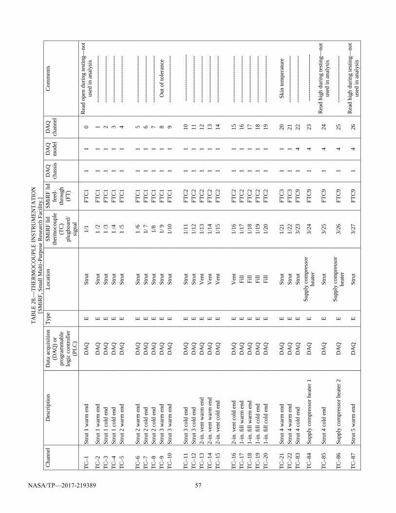
TA

BLE

28.—

THER

MO

CO

UPL

E IN

STR

UM

ENTA

TIO

N

[SM

iRF,

Sm

all M

ulti-

Purp

ose

Res

earc

h Fa

cilit

y.]

Cha

nnel

D

escr

iptio

n D

ata

acqu

isiti

on

(DA

Q) o

r pr

ogra

mm

able

lo

gic

cont

rolle

r (P

LC)

Type

Lo

catio

n SM

iRF

lid

ther

moc

oupl

e (T

C)

plug

boar

d/

sign

al

SMiR

F lid

fe

ed-

thro

ugh

(FT)

DA

Q

chas

sis

DA

Q

mod

el

DA

Q

chan

nel

Com

men

ts

TC–1

St

rut 1

war

m e

nd

DA

Q

E St

rut

1/1

FTC

1 1

1 0

Rea

d op

en d

urin

g te

stin

g—no

t us

ed in

ana

lysi

s TC

–2

Stru

t 1 w

arm

end

D

AQ

E

Stru

t 1

/2

FTC

1 1

1 1

----

----

----

----

----

----

TC

–3

Stru

t 1 c

old

end

D

AQ

E

Stru

t 1

/3

FTC

1 1

1 2

----

----

----

----

----

----

TC

–4

Stru

t 1 c

old

end

DA

Q

E St

rut

1 /4

FT

C1

1 1

3 --

----

----

----

----

----

--

TC–5

St

rut 2

war

m e

nd

DA

Q

E St

rut

1 /5

FT

C1

1 1

4 --

----

----

----

----

----

--

TC

–6

Stru

t 2 w

arm

end

D

AQ

E

Stru

t 1

/6

FTC

1 1

1 5

----

----

----

----

----

----

TC

–7

Stru

t 2 c

old

end

D

AQ

E

Stru

t 1/

7

FTC

1 1

1 6

----

----

----

----

----

----

TC

–8

Stru

t 2 c

old

end

DA

Q

E St

rut

1/8

FTC

1 1

1 7

----

----

----

----

----

----

TC

–9

Stru

t 3 w

arm

end

D

AQ

E

Stru

t 1/

9

FTC

1 1

1 8

Out

of t

oler

ance

TC

–10

Stru

t 3 w

arm

end

D

AQ

E

Stru

t 1/

10

FTC

1 1

1 9

----

----

----

----

----

----

TC–1

1 St

rut 3

col

d en

d

DA

Q

E St

rut

1/11

FT

C2

1 1

10

----

----

----

----

----

----

TC

–12

Stru

t 3 c

old

end

DA

Q

E St

rut

1/12

FT

C2

1 1

11

----

----

----

----

----

----

TC

–13

2-in

. ven

t war

m e

nd

DA

Q

E V

ent

1/13

FT

C2

1 1

12

----

----

----

----

----

----

TC

–14

2-in

. ven

t war

m e

nd

DA

Q

E V

ent

1/14

FT

C2

1 1

13

----

----

----

----

----

----

TC

–15

2-in

. ven

t col

d en

d D

AQ

E

Ven

t 1/

15

FTC

2 1

1 14

--

----

----

----

----

----

--

TC

–16

2-in

. ven

t col

d en

d D

AQ

E

Ven

t 1/

16

FTC

2 1

1 15

--

----

----

----

----

----

--

TC–1

7 1-

in. f

ill w

arm

end

D

AQ

E

Fill

1/17

FT

C2

1 1

16

----

----

----

----

----

----

TC

–18

1-in

. fill

war

m e

nd

DA

Q

E Fi

ll 1/

18

FTC

2 1

1 17

--

----

----

----

----

----

--

TC–1

9 1-

in. f

ill c

old

end

DA

Q

E Fi

ll 1/

19

FTC

2 1

1 18

--

----

----

----

----

----

--

TC–2

0 1-

in. f

ill c

old

end

DA

Q

E Fi

ll 1/

20

FTC

2 1

1 19

--

----

----

----

----

----

--

TC

–21

Stru

t 4 w

arm

end

D

AQ

E

Stru

t 1/

21

FTC

3 1

1 20

Sk

in te

mpe

ratu

re

TC–2

2 St

rut 4

war

m e

nd

DA

Q

E St

rut

1/22

FT

C3

1 1

21

----

----

----

----

----

----

TC

–83

Stru

t 4 c

old

end

DA

Q

E St

rut

3/23

FT

C9

1 4

22

----

----

----

----

----

----

TC–8

4 Su

pply

com

pres

sor h

eate

r 1

DA

Q

E Su

pply

com

pres

sor

heat

er

3/24

FT

C9

1 4

23

----

----

----

----

----

----

TC–8

5 St

rut 4

col

d en

d D

AQ

E

Stru

t 3/

25

FTC

9 1

4 24

R

ead

high

dur

ing

test

ing—

not

used

in a

naly

sis

TC–8

6 Su

pply

com

pres

sor h

eate

r 2

DA

Q

E Su

pply

com

pres

sor

heat

er

3/26

FT

C9

1 4

25

----

----

----

----

----

----

TC–8

7 St

rut 5

war

m e

nd

DA

Q

E St

rut

3/27

FT

C9

1 4

26

Rea

d hi

gh d

urin

g te

stin

g—no

t us

ed in

ana

lysi

s

NASA/TP—2017-219389 57

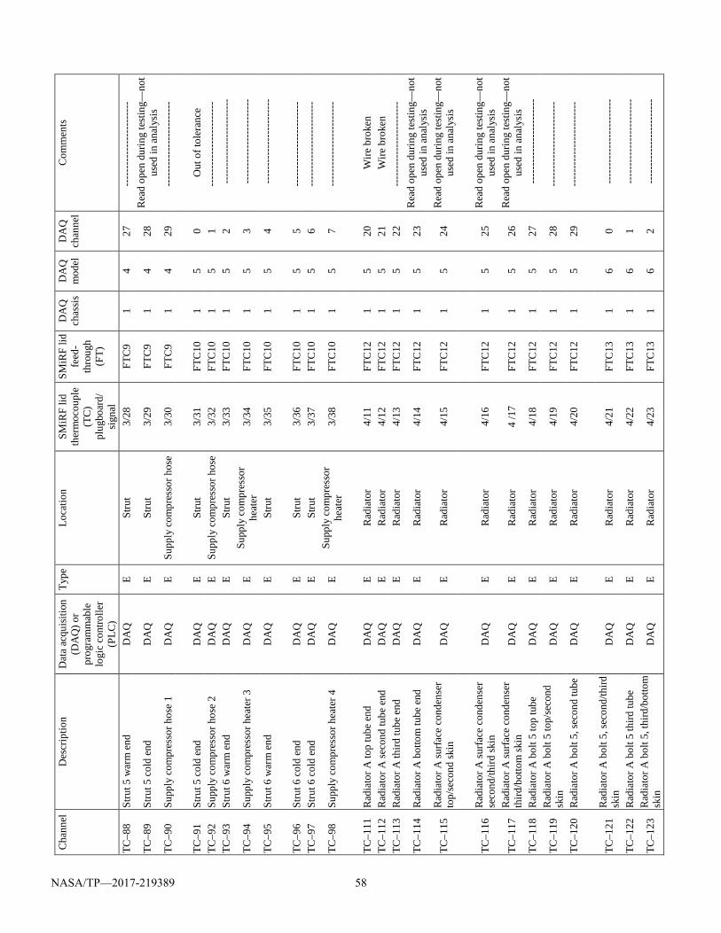
C

hann

el

Des

crip

tion

Dat

a ac

quis

ition

(D

AQ

) or

prog

ram

mab

le

logi

c co

ntro

ller

(PLC

)

Type

Lo

catio

n SM

iRF

lid

ther

moc

oupl

e (T

C)

plug

boar

d/

sign

al

SMiR

F lid

fe

ed-

thro

ugh

(FT)

DA

Q

chas

sis

DA

Q

mod

el

DA

Q

chan

nel

Com

men

ts

TC–8

8 St

rut 5

war

m e

nd

DA

Q

E St

rut

3/28

FT

C9

1 4

27

----

----

----

----

----

----

TC–8

9 St

rut 5

col

d en

d D

AQ

E

Stru

t 3/

29

FTC

9 1

4 28

R

ead

open

dur

ing

test

ing—

not

used

in a

naly

sis

TC–9

0 Su

pply

com

pres

sor h

ose

1 D

AQ

E

Supp

ly c

ompr

esso

r hos

e 3/

30

FTC

9 1

4 29

--

----

----

----

----

----

--

TC

–91

Stru

t 5 c

old

end

DA

Q

E St

rut

3/31

FT

C10

1

5 0

Out

of t

oler

ance

TC

–92

Supp

ly c

ompr

esso

r hos

e 2

DA

Q

E Su

pply

com

pres

sor h

ose

3/32

FT

C10

1

5 1

----

----

----

----

----

----

TC

–93

Stru

t 6 w

arm

end

D

AQ

E

Stru

t 3/

33

FTC

10

1 5

2 --

----

----

----

----

----

--

TC–9

4 Su

pply

com

pres

sor h

eate

r 3

DA

Q

E Su

pply

com

pres

sor

heat

er

3/34

FT

C10

1

5 3

----

----

----

----

----

----

TC–9

5 St

rut 6

war

m e

nd

DA

Q

E St

rut

3/35

FT

C10

1

5 4

----

----

----

----

----

----

TC–9

6 St

rut 6

col

d en

d D

AQ

E

Stru

t 3/

36

FTC

10

1 5

5 --

----

----

----

----

----

--

TC–9

7 St

rut 6

col

d en

d D

AQ

E

Stru

t 3/

37

FTC

10

1 5

6 --

----

----

----

----

----

--

TC–9

8 Su

pply

com

pres

sor h

eate

r 4

DA

Q

E Su

pply

com

pres

sor

heat

er

3/38

FT

C10

1

5 7

----

----

----

----

----

----

TC

–111

R

adia

tor A

top

tube

end

D

AQ

E

Rad

iato

r 4/

11

FTC

12

1 5

20

Wire

bro

ken

TC–1

12

Rad

iato

r A se

cond

tube

end

D

AQ

E

Rad

iato

r 4/

12

FTC

12

1 5

21

Wire

bro

ken

TC–1

13

Rad

iato

r A th

ird tu

be e

nd

DA

Q

E R

adia

tor

4/13

FT

C12

1

5 22

--

----

----

----

----

----

--

TC–1

14

Rad

iato

r A b

otto

m tu

be e

nd

DA

Q

E R

adia

tor

4/14

FT

C12

1

5 23

R

ead

open

dur

ing

test

ing—

not

used

in a

naly

sis

TC–1

15

Rad

iato

r A su

rface

con

dens

er

top/

seco

nd sk

in

DA

Q

E R

adia

tor

4/15

FT

C12

1

5 24

R

ead

open

dur

ing

test

ing—

not

used

in a

naly

sis

TC–1

16

Rad

iato

r A su

rface

con

dens

er

seco

nd/th

ird sk

in

DA

Q

E R

adia

tor

4/16

FT

C12

1

5 25

R

ead

open

dur

ing

test

ing—

not

used

in a

naly

sis

TC–1

17

Rad

iato

r A su

rface

con

dens

er

third

/bot

tom

skin

D

AQ

E

Rad

iato

r 4

/17

FTC

12

1 5

26

Rea

d op

en d

urin

g te

stin

g—no

t us

ed in

ana

lysi

s TC

–118

R

adia

tor A

bol

t 5 to

p tu

be

DA

Q

E R

adia

tor

4/18

FT

C12

1

5 27

--

----

----

----

----

----

--

TC–1

19

Rad

iato

r A b

olt 5

top/

seco

nd

skin

D

AQ

E

Rad

iato

r 4/

19

FTC

12

1 5

28

----

----

----

----

----

----

TC–1

20

Rad

iato

r A b

olt 5

, sec

ond

tube

D

AQ

E

Rad

iato

r 4/

20

FTC

12

1 5

29

----

----

----

----

----

----

TC–1

21

Rad

iato

r A b

olt 5

, sec

ond/

third

sk

in

DA

Q

E R

adia

tor

4/21

FT

C13

1

6 0

----

----

----

----

----

----

TC–1

22

Rad

iato

r A b

olt 5

third

tube

D

AQ

E

Rad

iato

r 4/

22

FTC

13

1 6

1 --

----

----

----

----

----

--

TC–1

23

Rad

iato

r A b

olt 5

, thi

rd/b

otto

m

skin

D

AQ

E

Rad

iato

r 4/

23

FTC

13

1 6

2 --

----

----

----

----

----

--

NASA/TP—2017-219389 58

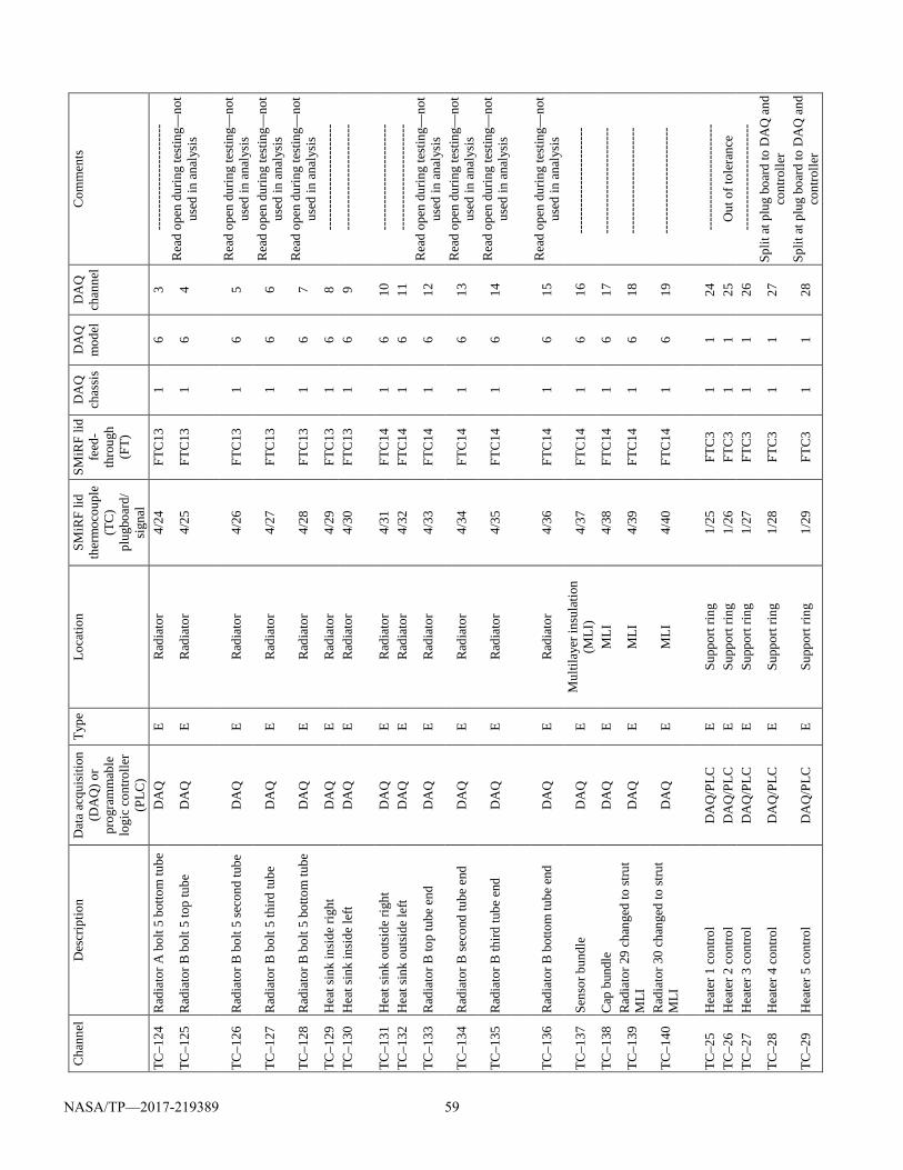
C

hann

el

Des

crip

tion

Dat

a ac

quis

ition

(D

AQ

) or

prog

ram

mab

le

logi

c co

ntro

ller

(PLC

)

Type

Lo

catio

n SM

iRF

lid

ther

moc

oupl

e (T

C)

plug

boar

d/

sign

al

SMiR

F lid

fe

ed-

thro

ugh

(FT)

DA

Q

chas

sis

DA

Q

mod

el

DA

Q

chan

nel

Com

men

ts

TC–1

24

Rad

iato

r A b

olt 5

bot

tom

tube

D

AQ

E

Rad

iato

r 4/

24

FTC

13

1 6

3 --

----

----

----

----

----

--

TC–1

25

Rad

iato

r B b

olt 5

top

tube

D

AQ

E

Rad

iato

r 4/

25

FTC

13

1 6

4 R

ead

open

dur

ing

test

ing—

not

used

in a

naly

sis

TC–1

26

Rad

iato

r B b

olt 5

seco

nd tu

be

DA

Q

E R

adia

tor

4/26

FT

C13

1

6 5

Rea

d op

en d

urin

g te

stin

g—no

t us

ed in

ana

lysi

s

TC–1

27

Rad

iato

r B b

olt 5

third

tube

D

AQ

E

Rad

iato

r 4/

27

FTC

13

1 6

6 R

ead

open

dur

ing

test

ing—

not

used

in a

naly

sis

TC–1

28

Rad

iato

r B b

olt 5

bot

tom

tube

D

AQ

E

Rad

iato

r 4/

28

FTC

13

1 6

7 R

ead

open

dur

ing

test

ing—

not

used

in a

naly

sis

TC–1

29

Hea

t sin

k in

side

righ

t D

AQ

E

Rad

iato

r 4/

29

FTC

13

1 6

8 --

----

----

----

----

----

--

TC–1

30

Hea

t sin

k in

side

left

DA

Q

E R

adia

tor

4/30

FT

C13

1

6 9

----

----

----

----

----

----

TC–1

31

Hea

t sin

k ou

tsid

e rig

ht

DA

Q

E R

adia

tor

4/31

FT

C14

1

6 10

--

----

----

----

----

----

--

TC–1

32

Hea

t sin

k ou

tsid

e le

ft D

AQ

E

Rad

iato

r 4/

32

FTC

14

1 6

11

----

----

----

----

----

----

TC–1

33

Rad

iato

r B to

p tu

be e

nd

DA

Q

E R

adia

tor

4/33

FT

C14

1

6 12

R

ead

open

dur

ing

test

ing—

not

used

in a

naly

sis

TC–1

34

Rad

iato

r B se

cond

tube

end

D

AQ

E

Rad

iato

r 4/

34

FTC

14

1 6

13

Rea

d op

en d

urin

g te

stin

g—no

t us

ed in

ana

lysi

s

TC–1

35

Rad

iato

r B th

ird tu

be e

nd

DA

Q

E R

adia

tor

4/35

FT

C14

1

6 14

R

ead

open

dur

ing

test

ing—

not

used

in a

naly

sis

TC–1

36

Rad

iato

r B b

otto

m tu

be e

nd

DA

Q

E R

adia

tor

4/36

FT

C14

1

6 15

R

ead

open

dur

ing

test

ing—

not

used

in a

naly

sis

TC–1

37

Sens

or b

undl

e D

AQ

E

Mul

tilay

er in

sula

tion

(MLI

) 4/

37

FTC

14

1 6

16

----

----

----

----

----

----

TC–1

38

Cap

bun

dle

DA

Q

E M

LI

4/38

FT

C14

1

6 17

--

----

----

----

----

----

--

TC–1

39

Rad

iato

r 29

chan

ged

to st

rut

MLI

D

AQ

E

MLI

4/

39

FTC

14

1 6

18

----

----

----

----

----

----

TC–1

40

Rad

iato

r 30

chan

ged

to st

rut

MLI

D

AQ

E

MLI

4/

40

FTC

14

1 6

19

----

----

----

----

----

----

TC

–25

Hea

ter 1

con

trol

DA

Q/P

LC

E Su

ppor

t rin

g 1/

25

FTC

3 1

1 24

--

----

----

----

----

----

--

TC–2

6 H

eate

r 2 c

ontro

l D

AQ

/PLC

E

Supp

ort r

ing

1/26

FT

C3

1 1

25

Out

of t

oler

ance

TC

–27

Hea

ter 3

con

trol

DA

Q/P

LC

E Su

ppor

t rin

g 1/

27

FTC

3 1

1 26

--

----

----

----

----

----

--

TC–2

8 H

eate

r 4 c

ontro

l D

AQ

/PLC

E

Supp

ort r

ing

1/28

FT

C3

1 1

27

Split

at p

lug

boar

d to

DA

Q a

nd

cont

rolle

r

TC–2

9 H

eate

r 5 c

ontro

l D

AQ

/PLC

E

Supp

ort r

ing

1/29

FT

C3

1 1

28

Split

at p

lug

boar

d to

DA

Q a

nd

cont

rolle

r

NASA/TP—2017-219389 59

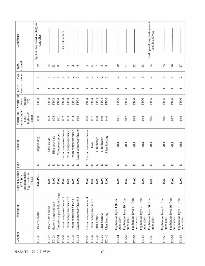
C

hann

el

Des

crip

tion

Dat

a ac

quis

ition

(D

AQ

) or

prog

ram

mab

le

logi

c co

ntro

ller

(PLC

)

Type

Lo

catio

n SM

iRF

lid

ther

moc

oupl

e (T

C)

plug

boar

d/

sign

al

SMiR

F lid

fe

ed-

thro

ugh

(FT)

DA

Q

chas

sis

DA

Q

mod

el

DA

Q

chan

nel

Com

men

ts

TC–3

0 H

eate

r 6 c

ontro

l D

AQ

/PLC

E

Supp

ort r

ing

1/30

FT

C3

1 1

29

Split

at p

lug

boar

d to

DA

Q a

nd

cont

rolle

r

TC–2

3 H

eate

r 1 st

rut c

levi

s D

AQ

E

Stru

t cle

vis

1/23

FT

C3

1 1

22

----

----

----

----

----

----

TC

–24

Hea

ter 1

ring

stru

t bas

e D

AQ

E

Rin

g st

rut b

ase

1/24

FT

C3

1 1

23

----

----

----

----

----

----

TC

–31

Com

pres

sor p

ipe

befo

re fl

ange

D

AQ

E

Com

pres

sor p

ipe

1/31

FT

C4

1 2

0 --

----

----

----

----

----

--

TC–3

2 R

etur

n co

mpr

esso

r hea

ter 1

D

AQ

E

Ret

urn

com

pres

sor h

eate

r 1/

32

FTC

4 1

2 1

Out

of t

oler

ance

TC

–33

Ret

urn

com

pres

sor h

eate

r 2

DA

Q

E R

etur

n co

mpr

esso

r hea

ter

1/33

FT

C4

1 2

2 --

----

----

----

----

----

--

TC–3

4 R

etur

n co

mpr

esso

r hos

e 1

DA

Q

E R

etur

n co

mpr

esso

r hos

e 1/

34

FTC

4 1

2 3

----

----

----

----

----

----

TC

–35

Ret

urn

com

pres

sor h

eate

r 3

DA

Q

E R

etur

n co

mpr

esso

r hea

ter

1/35

FT

C4

1 2

4 --

----

----

----

----

----

--

TC

–36

Ret

urn

com

pres

sor h

eate

r 4

DA

Q

E R

etur

n co

mpr

esso

r hea

ter

1/36

FT

C4

1 2

5 --

----

----

----

----

----

--

TC–3

7 R

etur

n co

mpr

esso

r hos

e 2

DA

Q

E H

ose

1/37

FT

C4

1 2

6 --

----

----

----

----

----

--

TC–3

8 Fi

lter h

eate

r 1

DA

Q

E Fi

lter h

eate

r 1/

38

FTC

4 1

2 7

----

----

----

----

----

----

TC

–39

Filte

r hea

ter 2

D

AQ

E

Filte

r hea

ter

1/39

FT

C4

1 2

8 --

----

----

----

----

----

--

TC–4

0 Fi

lter h

ousin

g D

AQ

E

Filte

r hou

sing

1/40

FT

C4

1 2

9 --

----

----

----

----

----

--

TC–5

1 To

p bl

anke

t lay

er 1

(fro

m

oute

r sid

e)

DA

Q

E M

LI

2/11

FT

C6

1 2

20

----

----

----

----

----

----

TC–5

2 To

p bl

anke

t lay

er 1

9 (fr

om

oute

r sid

e)

DA

Q

E M

LI

2/12

FT

C6

1 2

21

----

----

----

----

----

----

TC–5

3 To

p bl

anke

t lay

er 3

7 (fr

om

oute

r sid

e)

DA

Q

E M

LI

2/13

FT

C6

1 2

22

----

----

----

----

----

----

TC–5

4 To

p bl

anke

t lay

er 7

1 (fr

om

oute

r sid

e)

DA

Q

E M

LI

2/14

FT

C6

1 2

23

----

----

----

----

----

----

TC–5

5 To

p bl

anke

t lay

er 6

6 (fr

om

oute

r sid

e)

DA

Q

E M

LI

2/15

FT

C6

1 2

24

Rea

d op

en d

urin

g te

stin

g—no

t us

ed in

ana

lysi

s

TC–5

6 To

p bl

anke

t lay

er 6

1 (fr

om

oute

r sid

e)

DA

Q

E M

LI

2/16

FT

C6

1 2

25

----

----

----

----

----

----

TC–5

7 To

p bl

anke

t lay

er 5

6 (fr

om

oute

r sid

e)

DA

Q

E M

LI

2/17

FT

C6

1 2

26

----

----

----

----

----

----

TC–5

8 To

p bl

anke

t lay

er 5

1 (fr

om

oute

r sid

e)

DA

Q

E M

LI

2/18

FT

C6

1 2

27

----

----

----

----

----

----

NASA/TP—2017-219389 60

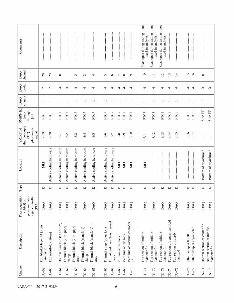
C

hann

el

Des

crip

tion

Dat

a ac

quis

ition

(D

AQ

) or

prog

ram

mab

le

logi

c co

ntro

ller

(PLC

)

Type

Lo

catio

n SM

iRF

lid

ther

moc

oupl

e (T

C)

plug

boar

d/

sign

al

SMiR

F lid

fe

ed-

thro

ugh

(FT)

DA

Q

chas

sis

DA

Q

mod

el

DA

Q

chan

nel

Com

men

ts

TC–5

9 To

p bl

anke

t lay

er 4

4 (fr

om

oute

r sid

e)

DA

Q

E M

LI

2/19

FT

C6

1 2

28

----

----

----

----

----

----

TC–6

0 To

p m

anifo

ld (r

etur

n)

DA

Q

E A

ctiv

e co

olin

g ha

rdw

are

2/20

FT

C6

1 2

29

----

----

----

----

----

----

TC–6

1 B

otto

m m

anifo

ld (S

UPP

LY)

DA

Q

E A

ctiv

e co

olin

g ha

rdw

are

3/1

FTC

7 1

4 0

----

----

----

----

----

----

TC–6

2 Th

erm

al b

lock

(2-in

. pip

e)—

clam

p D

AQ

E

Act

ive

cool

ing

hard

war

e 3/

2 FT

C7

1 4

1 --

----

----

----

----

----

--

TC–6

3 Th

erm

al b

lock

(2-in

. pip

e)—

stra

p D

AQ

E

Act

ive

cool

ing

hard

war

e 3/

3 FT

C7

1 4

2 --

----

----

----

----

----

--

TC–6

4 Th

erm

al b

lock

(man

ifold

)—cl

amp

DA

Q

E A

ctiv

e co

olin

g ha

rdw

are

3/4

FTC

7 1

4 3

----

----

----

----

----

----

TC–6

5 Th

erm

al b

lock

(man

ifold

)—st

rap

DA

Q

E A

ctiv

e co

olin

g ha

rdw

are

3/5

FTC

7 1

4 4

----

----

----

----

----

----

TC

–66

Ther

mal

stra

p (o

uter

foil)

D

AQ

E

Act

ive

cool

ing

hard

war

e 3/

6 FT

C7

1 4

5 --

----

----

----

----

----

--

TC–6

7 To

p of

tank

nea

r 2-in

. the

rmal

bl

ock

DA

Q

E A

ctiv

e co

olin

g ha

rdw

are

3/7

FTC

7 1

4 6

----

----

----

----

----

----

TC–6

8 Fi

ll lin

e at

test

tank

D

AQ

E

MLI

3/

8 FT

C7

1 4

7 --

----

----

----

----

----

--

TC–6

9 V

ent l

ine

at te

st ta

nk

DA

Q

E M

LI

3/9

FTC

7 1

4 8

----

----

----

----

----

----

TC–7

0 V

ent l

ine

at v

acuu

m c

ham

ber

lid

DA

Q

E M

LI

3/10

FT

C7

1 4

9 --

----

----

----

----

----

--

TC–7

1 To

p se

ctio

n of

mid

dle

diam

eter

fin

DA

Q

E M

LI

3/11

FT

C8

1 4

10

Rea

d op

en d

urin

g te

stin

g—no

t us

ed in

ana

lysi

s

TC–7

2 To

p se

ctio

n of

mid

dle

diam

eter

fin

DA

Q

E --

----

----

----

----

----

--

3/12

FT

C8

1 4

11

Rea

d op

en d

urin

g te

stin

g—no

t us

ed in

ana

lysi

s

TC–7

3 To

p se

ctio

n of

mid

dle

diam

eter

fin

DA

Q

E --

----

----

----

----

----

--

3/13

FT

C8

1 4

12

Rea

d op

en d

urin

g te

stin

g—no

t us

ed in

ana

lysi

s TC

–74

Top

sect

ion

of re

turn

man

ifold

D

AQ

E

----

----

----

----

----

----

3/

14

FTC

8 1

4 13

--

----

----

----

----

----

--

TC–7

5 To

p se

ctio

n of

supp

ly

man

ifold

D

AQ

E

----

----

----

----

----

----

3/

15

FTC

8 1

4 14

--

----

----

----

----

----

--

TC

–76

Ulte

m st

rap

at 8

0/20

D

AQ

E

----

----

----

----

----

----

3/

16

FTC

8 1

4 15

--

----

----

----

----

----

--

TC–7

7 U

ltem

stra

p at

cry

ocoo

ler

DA

Q

E --

----

----

----

----

----

--

3/17

FT

C8

1 4

16

----

----

----

----

----

----

TS–0

1 B

otto

m se

ctio

n of

cen

ter f

in

DA

Q

E B

otto

m o

f cry

oshr

oud

----

- Si

de F

T 1

3 0

----

----

----

----

----

----

TS–0

2 B

otto

m se

ctio

n of

mid

dle

diam

eter

fin

DA

Q

E B

otto

m o

f cry

oshr

oud

----

- Si

de F

T 1

3 1

----

----

----

----

----

----

NASA/TP—2017-219389 61

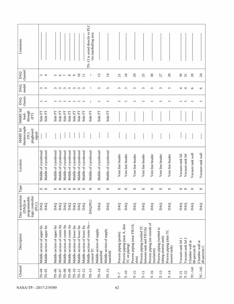
C

hann

el

Des

crip

tion

Dat

a ac

quis

ition

(D

AQ

) or

prog

ram

mab

le

logi

c co

ntro

ller

(PLC

)

Type

Lo

catio

n SM

iRF

lid

ther

moc

oupl

e (T

C)

plug

boar

d/

sign

al

SMiR

F lid

fe

ed-

thro

ugh

(FT)

DA

Q

chas

sis

DA

Q

mod

el

DA

Q

chan

nel

Com

men

ts

TS–0

4 M

iddl

e se

ctio

n of

upp

er fi

n D

AQ

E

Mid

dle

of c

ryos

hrou

d

----

- Si

de F

T 1

3 3

----

----

----

----

----

----

TS

–05

Mid

dle

sect

ion

of u

pper

fin

DA

Q

E M

iddl

e of

cry

oshr

oud

----

- Si

de F

T 1

3 4

----

----

----

----

----

----

TS–0

6 M

iddl

e se

ctio

n of

upp

er fi

n D

AQ

E

Mid

dle

of c

ryos

hrou

d --

---

Side

FT

1 3

5 --

----

----

----

----

----

--

TS–0

7 M

iddl

e se

ctio

n of

cen

ter f

in

DA

Q

E M

iddl

e of

cry

oshr

oud

----

- Si

de F

T 1

3 6

----

----

----

----

----

----

TS

–08

Mid

dle

sect

ion

of c

ente

r fin

D

AQ

E

Mid

dle

of c

ryos

hrou

d --

---

Side

FT

1 3

7 --

----

----

----

----

----

--

TS–0

9 M

iddl

e se

ctio

n of

cen

ter f

in

DA

Q

E M

iddl

e of

cry

oshr

oud

----

- Si

de F

T 1

3 8

----

----

----

----

----

----

TS

–10

Mid

dle

sect

ion

of lo

wer

fin

DA

Q

E M

iddl

e of

cry

oshr

oud

----

- Si

de F

T 1

3 9

----

----

----

----

----

----

TS

–11

Mid

dle

sect

ion

of lo

wer

fin

DA

Q

E M

iddl

e of

cry

oshr

oud

----

- Si

de F

T 1

3 10

--

----

----

----

----

----

--

TS–1

2 M

iddl

e se

ctio

n of

low

er fi

n D

AQ

E

Mid

dle

of c

ryos

hrou

d --

---

Side

FT

1 3

11

----

----

----

----

----

----

TS–1

3 M

iddl

e se

ctio

n of

cen

ter f

in—

cont

rol T

C

DA

Q/P

LC

E M

iddl

e of

cry

oshr

oud

----

- Si

de F

T --

--

--

TS

–13

is w

ired

dire

ctly

to P

LC

via

mar

shal

ling

area

TS–1

4 M

iddl

e se

ctio

n of

supp

ly

man

ifold

D

AQ

E

Mid

dle

of c

ryos

hrou

d --

---

Side

FT

1 3

13

----

----

----

----

----

----

TS–1

5 M

iddl

e se

ctio

n of

supp

ly

man

ifold

D

AQ

E

Mid

dle

of c

ryos

hrou

d --

---

Side

FT

1 3

14

----

----

----

----

----

----

T–

7 Pr

oces

s pip

ing

(pro

be)

DA

Q

E V

ent l

ine

head

er

----

- --

----

---

1 3

21

----

----

----

----

----

----

T–10

Pr

oces

s pip

ing

(nea

r A, s

kin

TC o

n pi

ping

) D

AQ

E

Ven

t lin

e he

ader

--

---

----

----

- 1

3 24

--

----

----

----

----

----

--

T–15

Pr

oces

s pip

ing

(nea

r FH

116,

sk

in)

DA

Q

E V

ent l

ine

head

er

----

- --

----

---

1 3

29

----

----

----

----

----

----

T–11

Pr

oces

s pip

ing

(wel

ded

TC

betw

een

tank

and

FH

116)

D

AQ

E

Ven

t lin

e he

ader

--

---

----

----

- 1

3 25

--

----

----

----

----

----

--

T–16

Pr

oces

s pip

ing

(on

outs

ide

of

insu

latio

n)

DA

Q

E V

ent l

ine

head

er

----

- --

----

---

1 3

30

----

----

----

----

----

----

T–13

Pr

oces

s pip

ing

(wel

ded

to

tubi

ng n

eare

st ta

nk)

DA

Q

E V

ent l

ine

head

er

----

- --

----

---

1 3

27

----

----

----

----

----

----

T–14

Pr

oces

s pip

ing

(ski

n TC

ne

ares

t tan

k)

DA

Q

E V

ent l

ine

head

er

----

- --

----

---

1 3

28

----

----

----

----

----

----

T–

21

Vac

uum

tank

lid

1 D

AQ

E

Vac

uum

tank

lid

----

- --

----

---

1 4

30

----

----

----

----

----

----

T–

22

Vac

uum

tank

lid

2 D

AQ

E

Vac

uum

tank

lid

----

- --

----

---

1 4

31

----

----

----

----

----

----

TC–1

41

Cha

mbe

r wal

l at

80-p

erce

nt B

D

AQ

E

Vac

uum

tank

wal

l --

---

----

----

- 1

6 20

--

----

----

----

----

----

--

TC–1

45

Cha

mbe

r wal

l at

40-p

erce

nt C

D

AQ

E

Vac

uum

tank

wal

l --

---

----

----

- 1

6 24

--

----

----

----

----

----

--

NASA/TP—2017-219389 62

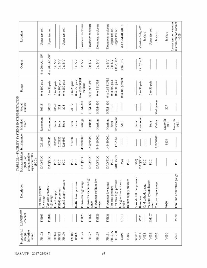
TA

BLE

29.—

FAC

ILIT

Y S

YST

EMS

INST

RU

MEN

TATI

ON

Pr

opor

tiona

l in

tegr

al

deriv

ativ

e na

me

LabV

IEW

TM

chan

nel

Des

crip

tion

Dat

a ac

quis

ition

(D

AQ

) or

prog

ram

mab

le

logi

c co

ntro

ller

(PLC

)

Seria

l num

ber

Man

ufac

-tu

rer

Mod

el

num

ber

Ran

ge

Out

put

Loca

tion

FH10

3 FH

103

Test

tank

pre

ssur

e—

low

rang

e D

AQ

/PLC

03

9119

3 R

osem

ount

30

51S

0 to

100

psi

a 4

to 2

0mA

/1–5

V

Upp

er te

st c

ell

FH10

9 FH

109

Test

tank

pre

ssur

e—

high

rang

e D

AQ

/PLC

04

6944

6 R

osem

ount

30

51S

0 to

50

psia

4

to 2

0mA

/1–5

V

Upp

er te

st c

ell

FH34

6 --

----

--

Liqu

id su

pply

PL

C

1823

27

Setra

20

5–2

0 to

50

psia

0

to 5

V

----

----

----

----

----

----

FH

382

----

----

FH

360

pres

sure

PL

C

5102

125

Setra

20

4 0

to 1

00 p

sia

0 to

5 V

--

----

----

----

----

----

--

FH17

0 --

----

--

Liqu

id su

pply

pre

ssur

e PL

C

6214

867

Setra

20

4 0

to 2

50 p

sia

0 to

5 V

U

pper

test

cel

l

FM

107

----

----

--

----

----

----

----

----

--

PLC

71

9788

Se

tra

205–

2 0

to 2

5 ps

ia

----

----

--

H

31A

--

----

--

H–1

6 D

ewar

pre

ssur

e PL

C

----

---

Setra

--

----

- 0

to 2

50 p

sia

0 to

5 V

--

----

----

----

----

----

--

FH12

5 FH

125

Flow

met

er h

igh

rang

e D

AQ

/PLC

48

8820

0001

H

astin

gs

HFM

–301

0

to 1

000

SCFH

m

etha

ne

0 to

5 V

Fl

owm

eter

enc

losu

re

FH12

7 FH

127

Flow

met

er m

ediu

m-h

igh

rang

e D

AQ

/PLC

14

5070

0001

H

astin

gs

HFM

–300

0

to 3

0 SL

PM

0 to

5 V

Fl

owm

eter

enc

losu

re

FH12

9 FH

129

Flow

met

er m

ediu

m-lo

w

rang

e D

AQ

/PLC

54

5460

0001

H

astin

gs

HFM

–300

0

to 5

SLP

M

0 to

5 V

Fl

owm

eter

enc

losu

re

FH13

1 FH

131

Flow

met

er lo

w ra

nge

DA

Q/P

LC

1494

8000

01

Has

tings

H

FM–3

00

0 to

0.6

6 SL

PM

0 to

5 V

Fl

owm

eter

enc

losu

re

FH12

1A

----

----

Te

st ta

nk p

ress

ure

PLC

Setra

--

----

- 0

to 3

00 p

sia

0 to

5 V

U

pper

test

cel

l FH

121B

--

----

--

Test

tank

hig

h pr

essu

re

B10

0 m

eter

17

0256

1 R

osem

ount

--

----

- 0

to 3

00 p

sia

4 to

20

mA

U

pper

test

cel

l

CA

P1

CA

P1

Line

gua

rd c

apac

itanc

e pr

obe

DA

Q

----

---

AM

I --

----

- 0

to 1

00 p

erce

nt

0 to

10

V

U.T

.C/M

AR

QR

–3

H36

9 --

----

--

Hel

ium

supp

ly p

ress

ure

PLC

--

----

-

--

----

----

----

----

----

--

XO

715

----

----

Sh

roud

chi

ll lin

e pr

essu

re

DA

Q

----

---

Setra

--

----

- --

----

----

----

--

----

----

--

----

----

----

----

----

--

V02

1 V

021

Bar

omet

er

DA

Q/P

LC

----

---

Ros

emou

nt

----

---

0 to

30

psia

4

to 2

0 m

A

Out

side

Bld

g. 4

02

V05

2 --

----

--

Col

d ca

thod

e ga

uge

PLC

--

----

-

In

shop

V05

8 FM

107

Vac

uum

syst

em h

eate

r re

turn

PL

C

----

---

Setra

--

----

- 0

to 5

0 ps

ia

----

----

--

Upp

er te

st c

ell

V00

5 --

----

--

Ther

moc

oupl

e ga

uge

----

----

LI

B00

202

Var

ian

Mul

tigau

ge

----

----

----

--

----

----

--

In sh

op

V05

0 --

----

--

V05

0 --

----

--

8134

G

ranv

ille

Phil

307

----

----

----

--

----

----

--

In sh

op

V07

0 V

070

Fore

Line

Con

vect

ron

gaug

e PL

C

----

----

--

Gra

nvill

e Ph

il --

----

- --

----

----

----

--

----

----

Lo

wer

test

cel

l vac

uum

in

stru

men

tatio

n ca

bine

t v1

09

NASA/TP—2017-219389 63

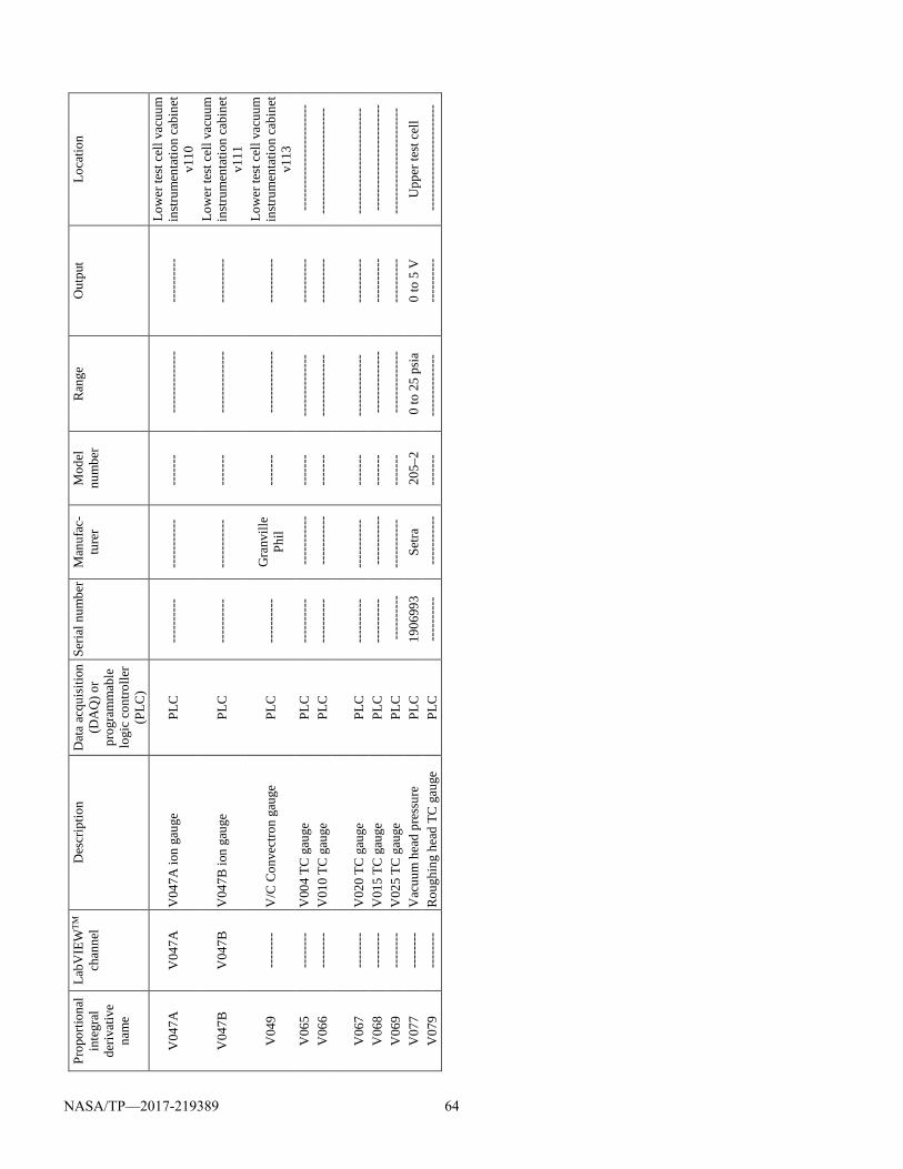
Pr

opor

tiona

l in

tegr

al

deriv

ativ

e na

me

LabV

IEW

TM

chan

nel

Des

crip

tion

Dat

a ac

quis

ition

(D

AQ

) or

prog

ram

mab

le

logi

c co

ntro

ller

(PLC

)

Seria

l num

ber

Man

ufac

-tu

rer

Mod

el

num

ber

Ran

ge

Out

put

Loca

tion

V04

7A

V04

7A

V04

7A io

n ga

uge

PLC

--

----

----

--

----

----

- --

----

- --

----

----

----

--

----

----

Lo

wer

test

cel

l vac

uum

in

stru

men

tatio

n ca

bine

t v1

10

V04

7B

V04

7B

V04

7B io

n ga

uge

PLC

--

----

----

--

----

----

- --

----

- --

----

----

----

--

----

----

Lo

wer

test

cel

l vac

uum

in

stru

men

tatio

n ca

bine

t v1

11

V04

9 --

----

--

V/C

Con

vect

ron

gaug

e PL

C

----

----

--

Gra

nvill

e Ph

il --

----

- --

----

----

----

--

----

----

Lo

wer

test

cel

l vac

uum

in

stru

men

tatio

n ca

bine

t v1

13

V06

5 --

----

--

V00

4 TC

gau

ge

PLC

--

----

----

--

----

----

- --

----

- --

----

----

----

--

----

----

--

----

----

----

----

----

--

V06

6 --

----

--

V01

0 TC

gau

ge

PLC

--

----

----

--

----

----

- --

----

- --

----

----

----

--

----

----

--

----

----

----

----

----

--

V06

7 --

----

--

V02

0 TC

gau

ge

PLC

--

----

----

--

----

----

- --

----

- --

----

----

----

--

----

----

--

----

----

----

----

----

--

V06

8 --

----

--

V01

5 TC

gau

ge

PLC

--

----

----

--

----

----

- --

----

- --

----

----

----

--

----

----

--

----

----

----

----

----

--

V06

9 --

----

--

V02

5 TC

gau

ge

PLC

--

----

----

--

----

----

- --

----

- --

----

----

----

--

----

----

--

----

----

----

----

----

--

V07

7 --

----

--

Vac

uum

hea

d pr

essu

re

PLC

19

0699

3 Se

tra

205–

2 0

to 2

5 ps

ia

0 to

5 V

U

pper

test

cel

l V

079

----

----

R

ough

ing

head

TC

gau

ge

PLC

--

----

----

--

----

----

- --

----

- --

----

----

----

--

----

----

--

----

----

----

----

----

--

NASA/TP—2017-219389 64

NASA/TP—2017-219389 65

References 1. Hoffman, Stephen J.; and Kaplan, David I., eds.: Human

Exploration of Mars: The Reference Mission of the NASA Mars Exploration Study Team. NASA SP–6107, 1997. http://ntrs.nasa.gov

2. Mars Architecture Steering Committee: Human Exploration of Mars Design Reference Architecture 5.0. NASA/SP—2009-566, 2009. http://ntrs.nasa.gov

3. Kittel, P.; Salerno, L.J.; and Plachta, D.W.: Cryocoolers for Human and Robotic Missions to Mars. Cryocoolers 15, Kluwer Academic/Plenum Publishers, New York, NY, 1998, pp. 815–821.

4. Kittel, P.; and Plachta, D.W.: Propellant Preservation for Mars Missions. Adv. Cryog. Eng., vol. 45(A), 2000, pp. 443–450.

5. Plachta, David W.: Hybrid Thermal Control Testing of a Cryogenic Propellant Tank. NASA/TM—1999-209389, 1999. http://ntrs.nasa.gov

6. Heydayat, Ali, et al.: Large Scale Demonstration of Liquid Hydrogen Storage With Zero Boiloff. AIP Conf. Proc., vol. 613, 2002, p. 1276.

7. Plachta, David: Results of an Advanced Development Zero Boil-Off Cryogenic Propellant Test. NASA/TM—2004-213390 (AIAA–2004–3837), 2004. http://ntrs.nasa.gov

8. Plachta, D.W., et al.: Cryogenic Propellant Boil-off Reduction System. Volume 53B Advances in Cryogenic Engineering, J.G. Weisend II, et al., eds, AIP Conf. Proc., vol. 985, 2008, pp. 1457–1466.

9. Feller, J., et al.: Analysis of Continuous Heat Exchangers for Cryogenic Boil-Off Reduction. Adv. Cryog. Eng., vol. 53, 2008, p. 401.

10. Feller, J.R., et al.: Distributed Cooling Techniques for Cryogenic Boil-Off Reduction Systems. Cryocoolers 15, Kluwer Academic/Plenum Publishers, New York, NY, 2009, p. 631.

11. Feller, J.R., et al.: Characterization of an Actively Cooled Metal Foil Thermal Radiation Shield. AIP Conf. Proc., vol. 1218, 2010, pp. 1187–1194.

12. Feller, J.R., et al.: Demonstration of a Cryogenic Boil-Off Reduction System Employing an Actively Cooled Thermal Radiation Shield. Kluwer Academic/Plenum Publishers, New York, NY, 2010, p. 601.

13. Christie, R.J., et al.: Broad Area Cooler Concepts for Cryogenic Propellant Tanks. Thermal & Fluids Analysis Workshop, Hampton, VA, 2011.

14. Gully, W., et al.: Ball Aerospace Next Generation Two-Stage 35 K Coolers: The SB235 and SB235E. Cryocoolers 14, Kluwer Academic/Plenum Publishers, New York, NY, 2007, p. 49.

15. Jaco, C.; Nguyen, T.; and Tward, E.: High Capacity Two-Stage Coaxial Pulse Tube Cooler. AIP Conf. Proc., vol. 985, 2008, p. 530.

16. Dietz, Anthony: A Turbo-Brayton Cryocooler for Aircraft Superconducting Systems. NASA/TM—2014-218497, 2014. http://ntrs.nasa.gov

17. Creare, Inc.: Scaling Study. NASA Contract NNG12LN29P, 2012.

18. Hochstein, John I.; Ji, Hyun-Chul; and Aydelott, John C.: Prediction of Self-Pressurization Rate of Cryogenic Propellant Tankage. J. Propulsion, vol. 6, no. 1, pp. 1990, pp. 11–17.

19. Plachta, David; and Guzik, Monica: Cryogenic Boil-Off Reduction System Scaling Study. Cryogenics, vol. 60, 2014, pp. 62–67.

20. Knoll, Richard H.; Stochl, Robert J.; and Sanabria, Rafael: A Review of Candidate Multilayer Insulation Systems for Potential Use on Wet-Launched LH2 Tankage for the Space Exploration Initiative Lunar Missions. NASA TM–104493 (AIAA–91–2176), 1991.

21. Jurns, John M.; and Kudlac, Maureen T.: NASA Glenn Research Center Creek Road Complex—Cryogenic Testing Facilities. Cryogenics, vol. 46, 2006, pp. 98–104.

22. Plachta, D.W.; Johnson, W.L.; and Feller, J.R.: Cryogenic Boil-Off Reduction System Testing. Presented at the 50th AIAA/ASME/SAE/ASEE Joint Propulsion Conference, Cleveland, OH, 2014.

23. ASTM E595–93: Standard Test Method for Mass Loss and Collected Volatile Condensable Materials from Outgassing in a Vacuum Environment. ASTM International, West Conshohocken, PA, 1993.

24. Johnson, Wesley L.; Kelly, Andrew O.; and Jumper, Kevin M.: Two Dimensional Heat Transfer around Penetrations in Multilayer Insulation. NASA/TP—2012-216315, 2012. http://ntrs.nasa.gov

25. Martin, J.J.; and Hastings, L.: Large-Scale Liquid Hydrogen Testing of a Variable Density Multilayer Insulation With a Foam Substrate. NASA/TM—2001-211089, 2001. http://ntrs.nasa.gov

26. ter Brake, H.J.M.: Low-Power Cryocooler Survey. Cryogenics, vol. 42, no. 11, 2002, pp. 705-718.

27. Lemmon, Eric W.; Huber, Marcia L.; and McLinden, Mark O.: NIST Reference Fluid Thermodynamic and Transport Properties—REFPROP. NIST Standard Reference Database 23, Version 8.0, 2007.

28. Hasan, M.M.; Lin, C.S.; and Van Dresar, N.T.: Self-Pressurization of a Flightweight Liquid Hydrogen Storage Tank Subjected to Low Heat Flux. NASA TM–103804, 1991. http://ntrs.nasa.gov









NASA/TP—2017-219389 66

29. Van Dresar, N.T.; Lin, C.S.; and Hasan, M.M.: Self-Pressurization of a Flightweight Liquid Hydrogen Tank: Effects of Fill Level at Low Wall Heat Flux. NASA TM–105411 (AIAA–92–0818), 1992. http://ntrs.nasa.gov

30. Van Dresar, Neil T.: Liquid Oxygen Thermodynamic Vent System Testing with Helium Pressurization. NASA/TP—2014-216633, 2014. http://ntrs.nasa.gov

31. National Institute of Standards and Technology: Material Properties: 304 Stainless (UNS S30400). http://www.cryogenics.nist.gov/MPropsMAY/304Stainless/304Stainless_rev.htm Accessed Oct. 27, 2016.

32. ASTM E408-71: Standard Test Methods for Total Normal Emittance of Surfaces Using Inspection-Meter Techniques. ASTM International, West Conshohocken, PA, 2008.

33. Sheldahl, The Red Book, 2016. http://www.sheldahl.com/ Documents/ShieldingMaterials/RedBook.pdf Accessed Nov. 1, 2016.

34. Howell, John R.; Pinar Menguc, M.; and Siegel, Robert: Thermal Radiation Heat Transfer. Fifth Edition, CRC Press, Philidelphia, PA, 2010.

35. Donabedian, Martin: Spacecraft Thermal Control Handbook. Volume 2, American Institute of Aeronautics and Astronautics/Aerospace Press, El Segundo, CA, 2003, p. 588.

36. Knoll, David, et al.: Evaluating Cryostat Performance for Naval Applications. AIP Conf. Proc., vol. 1434, 2012, p. 265.

37. Hinckley, R.: Liquid Propellant Losses During Space Flight. NASA CR–53336, 1964.

38. Zagarola, Mark: Turbo-Brayton Cryocooler for NASA’s Liquid Oxygen Zero Boil-off Ground Test. TM–3293, Creare, 2012.

39. Sumner, Irving E.: Degradation of a Multilayer Insulation Due to Seam and a Penetration. NASA TN D–8229, 1976. http://ntrs.nasa.gov

40. Stochl, Robert J.: Basic Performance of a Multilayer Insulation System Containing 20 to 160 Layers. NASA TN D–7659, 1974. http://ntrs.nasa.gov

41. Keller, C.W.; Cunnington, G.R.; Glassford, A.P.: Thermal Performance of Multilayer Insulations. NASA CR–134477, 1974. http://ntrs.nasa.gov

42. Hastings, L.J.; Hedayat, A.; and Brown, T.M.: Analytical Modeling and Test Correlation of Variable Density Multilayer Insulation for Cryogenic Storage. NASA/TM—2004-213175, 2004. http://ntrs.nasa.gov

43. Johnson, Wesley Louis: Thermal Performance of Cryogenic Multilayer Insulation at Various Layer Spacings. Master’s Thesis, Univ. of Central Florida, 2010.

44. Johnson, Wesley; and Fesmire, James: Thermal Performance of Low Layer Density Multilayer Insulation Using Liquid Nitrogen. AIP Conf. Proc., vol. 1434, 2012, pp. 39-46.

45. Johnson, Wesley L., et al.: Tank Applied Testing of Load-Bearing Multilayer Insulation (LB–MLI). AIAA 2014-3581, 2014.

46. Tuttle, J., et al.: Thermal Properties of Double-Aluminized Kapton at Low Temperatures. AIP Conf. Proc., vol. 986, 2008, p. 34.



http://www.cryogenics.nist.gov/MPropsMAY/304Stainless/304Stainless_rev.htm

http://www.cryogenics.nist.gov/MPropsMAY/304Stainless/304Stainless_rev.htm

http://www.sheldahl.com/%20Documents/ShieldingMaterials/RedBook.pdf

http://www.sheldahl.com/%20Documents/ShieldingMaterials/RedBook.pdf



